Download - A three-dimensional electron spin resonance - Acert.

REVIEW OF SCIENTIFIC INSTRUMENTS VOLUME 75, NUMBER 9 SEPTEMBER 2004
A three-dimensional electron spin resonance microscope Aharon Blank, Curt R. Dunnam, Peter P. Borbat, and Jack H. Freeda)
National Biomedical Center for Advanced ESR Technology, Department of Chemistry and Chemical Biology, Cornell University, Ithaca, New York 14853
(Received 26 January 2004; accepted 3 June 2004; published 15 September 2004)
An electron spin resonance(ESR) imaging system, capable of acquiring three-dimensional(3D) images with a resolution of,10310330 mm in a few minutes of acquisition, is presented. This ESR microscope employs a commercial continuous wave ESR spectrometer, working at 9.1 GHz, in conjunction with a miniature imaging probe(resonator+gradient coils), gradient current drivers, and control software. The system can acquire the image of a smalls,1.531.530.25 mmdsample either by the modulated field gradient method, the projection reconstruction method, or by a combination of the two. A short discussion regarding the resolution of the modulated field gradient method in two-dimensional(2D) and 3D imaging is given. Detailed descriptions of the various system components are provided, along with several examples of 2D and 3D images that demonstrate the capabilities of the system. ©2004 American Institute of Physics.
[DOI: 10.1063/1.1786353]
e to
e, and nt of e the ide s. p- the
re- th a
ign of er by
mai
I. INTRODUCTION
Magnetic resonance is one of the most useful ima methodologies in materials science, biology, medicine.1–3While “traditionally” most of the applications o this technique have been associated with nuclear mag resonance(NMR) imaging, some of the more recent inve gations have been carried out by electron spin reson (ESR) imaging. The main ESR imaging(ESRI) efforts have been directed towards the observation of large biologica jects and the determination of their radical and oxygen centrations(by their effect on the radical linewidth).4–7 Such experiments, conductedin vivo, employ low fields o ,10 mT at low rf frequencies(which results in relativel low spin sensitivity), in order that the rf energy will penetr deeply into the biological object. Consequently, a typ voxel resolution in low frequency ESR experiments ,f2 mmg3. A different approach attempts to examine m smaller objects, with better spatial resolution. This type ESRI, directed towards microscopy(analogous to a NMR microscope8), can be employed at higher frequencies w improved sensitivity. Previous efforts in ESR microsc (ESRM) are scarce, and have resulted in an achievable lution of ,25–100mm for two-dimensional(2D) and three dimensional(3D) imaging.9–12 We recently achieved 2D im ages with a resolution of,f10 mmg2 by employing continuous wave(cw) ESR imaging utilizing a unique prob design.13
At present, ESRM is still far less developed(mainly due to technological issues)than NMR microscopy, for whic commercial instruments can provide 3D resolution ,10–20mm in small biological samples.8 Nevertheless ESR has many virtues compared to NMR, which sho make it the technique of choice with respect to magn
a)Author to whom correspondence should be addressed; electronic
[email protected]
Downloaded 28 Feb 2006 to 128.253.229.23. Redistribution subject to AIP
ic
e
- -
-
resonance imaging in many microscopic applications. example, the signal per spin in ESR is much greater th NMR,14 diffusion does not limit the resolution in the sh time scalessT1,T2’sø10 msd of the ESR measurements, u like NMR,15–18 ESR microresonators have a quality fac sQd of ,1000 compared to aQ,10 of the NMR microcoils,8,19 and the ESR line shape is more sensitiv dynamic effects—leading to richer information.20,21An additional factor is the lower cost of electromagnets used in as compared to the expensive superconducting magn NMR. These fundamental advantages, along with recen vances in ESR resonators, ESR spectrometer hardwar paramagnetic contrast solutions, warrant the developme a micron resolution ESR-based microscope to overcom resolution limitations of NMR microscopy and to prov complementary information to optical imaging modalitie
Our recent publication13 described several potential a plications for ESRM. It discussed in detail the theory and limiting factors of current ESRM technology, and it p sented some initial cw 2D imaging results performed wi high-permittivity miniature X-band s9.1 GHzd imaging probe. In the present work we discuss in detail the 3D microscope, which we have now developed. It is based o improved microstrip-fed high permittivity resonator, a m efficient 3D imaging gradient coils set, and improved con software. The sophisticated hardware and software des the microscope enables one to acquire the image eith the modulated field gradient(MFG) method22,23 or through the projection reconstruction(PR) imaging method.4,24 The microimaging system, suitable for use as an accessory many pre-existingX-band cw ESR spectrometers, provi magnetic resonance imaging capability with a voxel res tion down to,10310330 mm in a few minutes of acqu sition. To demonstrate the capability of the system, we s some imaging results for a solid sample of LiPc(Lithiuml:
Phthalocyanine radical)and for a solid form and a liquid
© 2004 American Institute of Physics
license or copyright, see http://rsi.aip.org/rsi/copyright.jsp
field ative dient sce- . The field
., lds, loca-
Rev. Sci. Instrum., Vol. 75, No. 9, September 2004 A 3D electron spin resonance microscope 3051
suspension of the synthesized LiNc–BuO(lithium octa- n-butoxy-substituted naphthalocyanine radical) micropar- ticulates.25
II. IMAGING METHOD
As noted above, the system can employ two diffe imaging methods to obtain the ESR image, within the fra work of cw acquisition. Some of the results presented in article were obtained with the PR method, which is prob the most common method used to acquirein vivo cw ESR images. This tomographic imaging technique has been scribed in detail in many previous publications,26 and we shall not elaborate on it in this article. Other results prese here were collected employing the MFG method. T method is less commonly employed since it is mainly ad tageous for microscopic applications. The MFG method been described previously,13,22,27with discussions of the im age acquisition technique, image signal-to-noise-ratio(SNR), and gradient coil requirements. Nevertheless, we inc here, for clarity, a short outline of this method, and a present a discussion of image resolution in 2D and 3D
aging, as a function of the modulated field gradient ampli-
ntire
-
d
tude, since this subject was not treated in previous pub tions.
The idea behind the MFG method is to over-modu the entire imaged sample, apart from a single voxel, which the ESR signal is obtained.22 The over-modulation o the sample is achieved by a set of gradient coils excited low frequency periodic current. These coils have a null point that can be swept in space by changing the rel current amplitude in each coil pair that produces the gra field. Let us analyze more quantitatively the imaging nario and obtain the image resolution for various cases time domain cw ESR signal in the case of conventional modulation is given by14
Sst,Bdd = S0 1
, s1d
whereDB1/2 is the full width half maximum(FWHM) of the ESR line;Bd=sB−B0d, whereB0 is the center of the line;Bm
is the modulation field amplitude(at a frequency of, e.g 100 kHz). The addition of sinusoidal modulation fie whose amplitudes depend both on time and the spatial
tion, results in the following spatial/time domain signal
Ssx,y,z,t,Bdd = S0 1
ysydsinsvyt + wyd + Bz zszdsinsvzt + wzdg2
. s2d
e
y s
e ay-
The modulated field gradients for theX, Y, andZ axes −Bz x,
Bz y, Bz
z, and of course the main modulation field,Bm, are all in the direction of the laboratoryZ axis(determined byB0). The field Bm is assumed to be homogeneous over the e sample volume(i.e., without any spatial dependence). The modulated field gradients are employed at much lower quency(e.g., 10–1000 Hz), and have the following spa dependence:
Bz xsxd = xGx, s3d
Bz ysyd = yGy,
Bz zszd = zGz.
It is thus clear that at the origin, wheresx,y,zd=s0,0,0d, Eq. (2) simplifies to Eq.(1). At other locations however, the ES signal is greatly attenuated, due to the over-modulation duced by the modulated gradients, and this attenuatio creases as the voxel is more distant from the origin. As m tioned above, the origin(null field point) can be moved b changing the ratio of the currents in the pairs of coils, w generate the modulated field gradients. The entire ima obtained by electronically scanning the imaged voxels w the sample volume.
We shall now address the issue of image resolu
- - -
.
should be finer asGx, Gy, andGz increase. In addition, th gradient modulation frequenciesvx, vy, vz, the relative phases between the gradient modulationswy,wzd, and also the time constant of the cw ESR signal acquisition affec image resolution. In order to provide quantitative analys these factors, we examine the ESR signal harmonics(with respect to the main modulation frequency). These harmonic are detected by the cw ESR spectrometer and are give(for the pth harmonic)by14
ap =E t=0
If Bz x=Bz
y=Bz z=0, then each harmonic signal has a spe
field, Bd=Bd m, for which it is maximal(for example, for th
second harmonic signal,Bd m=0). As one increasesBz
x, Bz y,
and/or Bz z, the amplitude ofap at Bd
m will decrease an quickly reach zero.22 To calculate the image resolution, fo specific signal harmonicp, we first find the fieldBd
m and then increaseBz
x, Bz y, and/orBz
z (depending on the dimensionalit), in our numerical calculations ofap, until ap at Bd
m become zero. The values ofBz
x, Bz y, and/orBz
z for whichap=0, divided by the applied gradient[Eq. (3)], provide us with the imag resolution. This resolution criterion is analogous to the R
28
nu- ts a lysis ent ).
the age the
yed
pa-
ging
the reso- quire MW ing , the
the . lock sing the
ions cs
e sam
3052 Rev. Sci. Instrum., Vol. 75, No. 9, September 2004 Blank et al.
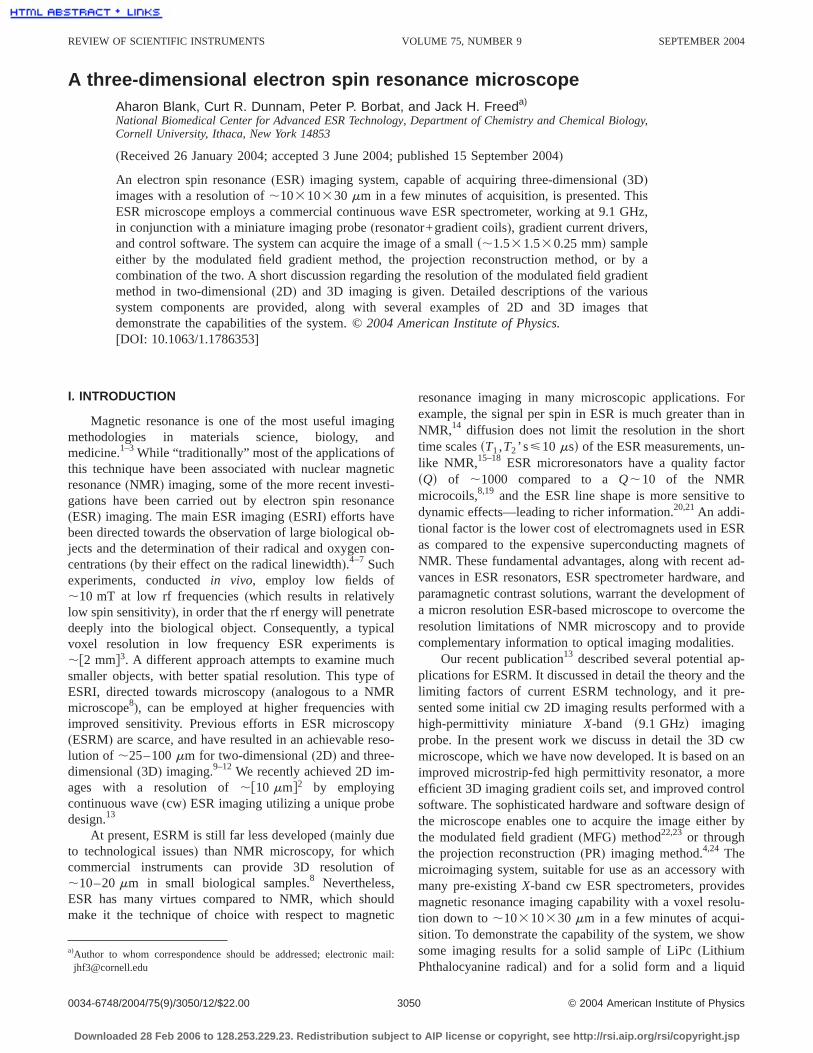
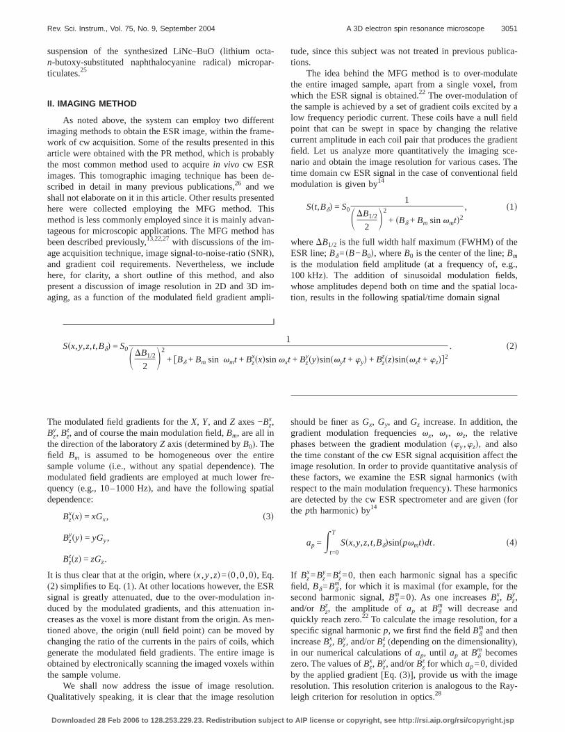
The calculations of the resolution were performed merically for several representative cases, and the resul shown in Fig. 1. We assumed for purposes of this ana that vx=vy=vz, (although the system can support differ frequencies for theX, Y, and Z gradient coils, see below Also Gx=Gy=Gz=G, and the integration time,T, in Eq. (4) was taken as the period time ofvx. The relative phases,wy, andwz, are determined according to the dimensionality of problem: When increasing the dimensionality of the im (e.g., from 1D to 2D), every point in space experiences added fields of more than one coil pair. This can lea “interference effects” as shown for the 2D example in F 2(a) and 2(b), which show how strong image artifacts created ifwy=0, since the resolution depends on the direc taken from the null point. To avoid such artifacts, one sh apply a phase difference between the modulated fields o different axes. In the 2D calculation of Fig. 1, we emplo an optimalwy=90°, and in the 3D example we appliedwy
=120°, wz=240°. This approach tends to minimize the s tial dependence of the resolution(i.e., image artifacts)by averaging out the positive and negative interference ef [cf. Figs. 2(c)and 2(d)]. Similar artifact cancellation can achieved by employing different modulated gradient quencies for each axis. Both methods(i.e., phase and/or fre quency variation among the imaging axes) can be employe
FIG. 1. Calculated image resolution for one, two, and three dimens employing the MFG method for the first(solid line) and second harmoni (dashed line)of the cw ESR signal. The FWHM radical linewidth andBm
are assumed to be 0.01 mT for all cases. The calculation assumes th applied gradient in all imaged dimensions.
in our imaging system(see below).
re
e
s
III. CONTINUOUS WAVE ESR MICROSCOPE
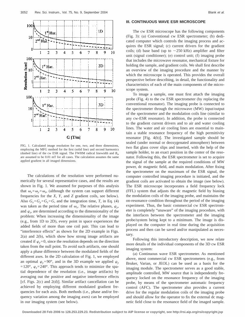
The cw ESR microscope has the following compon (Fig. 3): (a) Conventional cw ESR spectrometer;(b) dedi- cated computer which controls the imaging process an quires the ESR signal;(c) current drivers for the gradie coils; (d) base band(up to ,250 kHz) amplifier and filte unit (signal conditioner);(e) control unit; (f) imaging probe that includes the microwave resonator, mechanical fixtur holding the sample, and gradient coils. We shall first des an overview of the imaging procedure and the manne which the microscope is operated. This provides the ov perspective before describing, in detail, the functionality characteristics of each of the main components of the m scope system.
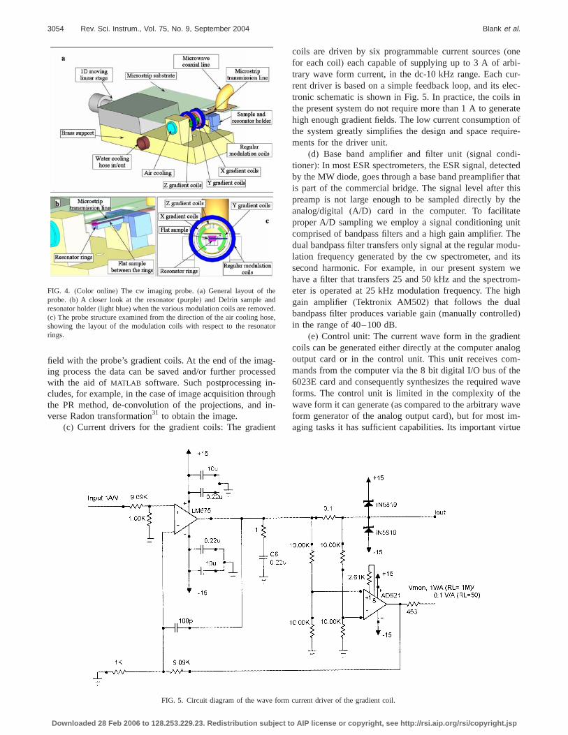
To image a sample, one must first attach the ima probe(Fig. 4) to the cw ESR spectrometer(by replacing the conventional resonator). The imaging probe is connected the spectrometer through the microwave(MW) input/outpu of the spectrometer and the modulation coils line(similar to any cw-ESR resonator). In addition, the probe is conne to the gradient current drivers and to air and water coo lines. The water and air cooling lines are essential to m tain a stable resonance frequency of the high permitt resonator[Fig. 4(b)]. The investigated sample should sealed(under normal or deoxygenated atmosphere) between two flat glass cover slips and inserted, with the help of sample holder, to an exact position in the center of the nator. Following this, the ESR spectrometer is set to ac the signal of the sample at the required conditions of power, dc magnetic field, and main modulation. After fix the spectrometer on the maximum of the ESR signal computer controlled imaging procedure is initiated, and gradient coils are activated to obtain the image(see below) The ESR microscope incorporates a field frequency (FFL) system that adjusts the dc magnetic field by bia the modulation coils of the imaging probe, and maintains on-resonance condition throughout the period of the ima experiment. Thus, the basic commercial cw ESR spect eter is completely “unaware” of the imaging procedure, w the interfaces between the spectrometer and the im probe/system being kept to a minimum. The image is played on the computer in real time during the acquis process and then can be saved and/or manipulated as sary.
Following this introductory description, we now rel more details of the individual components of the 3D cw E imaging system:
,
e
netic field close to the resonance field of the imaged sample.
is e. In i- low
y a e ven - and
l and
tire ppe
e rd-
th tion
ds ly mT,
es the cts in the 3D
The MW ESR signal returning from the imaging probe detected and preamplified at the spectrometer MW bridg our spectrometer(Varian E-12), we inserted prior to the d ode detection of the ESR signal from the resonator a noiseX-band preamplifier(Miteq AFS3-08001200-14-ULN). This amplifier improves the SNR of the spectrometer b factor of,5 and its amplification gains,25 dBdenables th AFC of the Varian bridge to lock on the returning signal e for low MW power s,1 mWd, that is common in our imag ing experiments(see below). The diode detected base b signal is directly fed from the bridge preamplifier(similar to the case of time resolved ESR measurements29) to a signa conditioning unit and then goes to the PC for sampling further analysis(see below).
(b) Control computer and imaging software: The en imaging process is controlled by a standard PC equi with two analog input+digital input/output(I/O) (National Instruments 6023E)and analog output(National Instrument 6713)cards. These cards enable arbitrary wave form ge tion and fast sampling of signals up to several hundred The digital analysis of the sampled diode detected ESR nal supersedes the need to employ a conventional lo amplifier while simultaneously obtaining all the ESR sig harmonics, in the correct phase, with respect to the modulation current.13,30 The current software version of t system is capable of acquiring 2D images at any givz location (3D slice selection). The 2D imaging methods t
FIG. 2. (a)The effect of two modulated field gradients applied for thex andy circles and the fields due to they coil pair are marked with6 with surroun will be stronger in the first and third quadrants, while tending to cancel small size situated at the origin of axes(point spread function) for 2D MFG Bm=0.01 mT,Gx=Gy=1 T/m. It is obvious that such a point spread f =90°. This phase difference between thex andy gradients leads to the min point spread function, which involved the simultaneous application ofx, y, image artifacts but still causes an appreciable anisotropy in the point MFG method.
can be employed are either the PR or the MFG method. Bot
d
- . - n
methods can in principle employ the MFG method for thZ slice selection(see below). It should be noted that the ha ware(probe+current drivers)also supports 3D imaging wi projection reconstruction and 4D spectral-spatial projec reconstruction that can be pursued in the future by upd the imaging control software. The control software(based on LABVIEW ) obtains the imaging parameters from the u These parameters include, for example, the number of p in the image(x andy), the current amplitude in the gradie coils, the wave form and frequency used in the modul gradient coils(e.g., sine, serrasoid, etc.), the image extent i mm, and parameters related to the functionality of the system. The software can also acquire the normal ESR s (first and second harmonics), by sweeping the magnet
s simultaneously. The fields due to thex coil pair are marked with6 without circles. It can be seen from the figure that ifwy=0, then the modulated fiel other in the second and fourth quadrants.(b) Image of a point target with infinite umingwy=0. Parameters used in this calculation are: linewidth of 0.01 on will result in bad artifacts in the image.(c) The same as(b), but with wy
ation of the artifacts in the point spread function.(d). A 2D cut through the 3D z gradients. The phase difference of 120° between each axis minimiz d function, which corresponds to some unavoidable anisotropic artifa
axe ding each , ass uncti imiz and
sprea
h FIG. 3. Block diagram of the 3D cw ESR microscope.
ag- ess in- ugh in-
ent
- ected r that this the
te nit The odu- d its
we trom- high l )
- rtue
nator
field with the probe’s gradient coils. At the end of the im ing process the data can be saved and/or further proc with the aid of MATLAB software. Such postprocessing cludes, for example, in the case of image acquisition thro the PR method, de-convolution of the projections, and verse Radon transformation31 to obtain the image.
(c) Current drivers for the gradient coils: The gradi
FIG. 4. (Color online) The cw imaging probe.(a) General layout of th probe. (b) A closer look at the resonator(purple) and Delrin sample an resonator holder(light blue) when the various modulation coils are remov (c) The probe structure examined from the direction of the air cooling h showing the layout of the modulation coils with respect to the reso rings.
FIG. 5. Circuit diagram of the wave form
ed
coils are driven by six programmable current sources(one for each coil)each capable of supplying up to 3 A of ar trary wave form current, in the dc-10 kHz range. Each rent driver is based on a simple feedback loop, and its tronic schematic is shown in Fig. 5. In practice, the coil the present system do not require more than 1 A to gen high enough gradient fields. The low current consumptio the system greatly simplifies the design and space req ments for the driver unit.
(d) Base band amplifier and filter unit(signal condi tioner): In most ESR spectrometers, the ESR signal, det by the MW diode, goes through a base band preamplifie is part of the commercial bridge. The signal level after preamp is not large enough to be sampled directly by analog/digital (A/D) card in the computer. To facilita proper A/D sampling we employ a signal conditioning u comprised of bandpass filters and a high gain amplifier. dual bandpass filter transfers only signal at the regular m lation frequency generated by the cw spectrometer, an second harmonic. For example, in our present system have a filter that transfers 25 and 50 kHz and the spec eter is operated at 25 kHz modulation frequency. The gain amplifier (Tektronix AM502) that follows the dua bandpass filter produces variable gain(manually controlled in the range of 40–100 dB.
,
dur rent ctua
e r of two - to b he y
x- elds
ect in d by d the
el ti- line nd
cy-
ns are ed
is that it reduces the overhead time in the imaging proce related to the calculation and generation of the diffe wave forms in the computer and thus shortens the a acquisition time by a factor of,2.
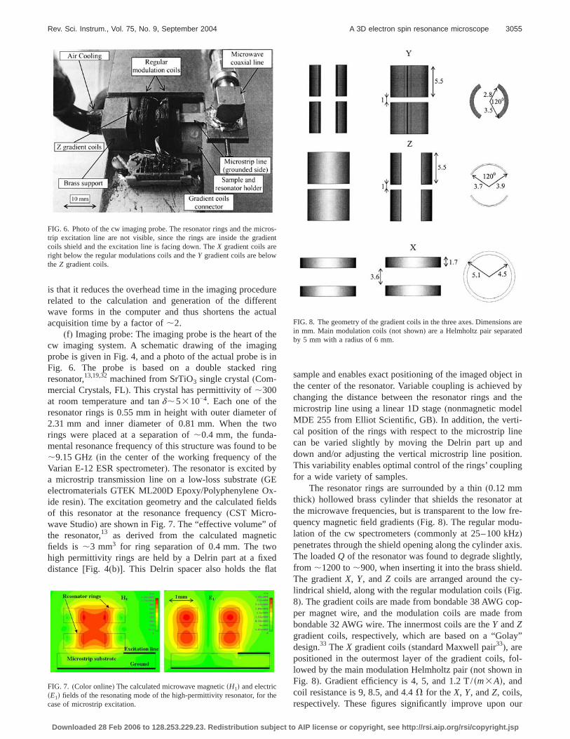
(f) Imaging probe: The imaging probe is the heart of cw imaging system. A schematic drawing of the imag probe is given in Fig. 4, and a photo of the actual probe Fig. 6. The probe is based on a double stacked resonator,13,19,32machined from SrTiO3 single crystal(Com- mercial Crystals, FL). This crystal has permittivity of,300 at room temperature and tand,5310−4. Each one of th resonator rings is 0.55 mm in height with outer diamete 2.31 mm and inner diameter of 0.81 mm. When the rings were placed at a separation of,0.4 mm, the funda mental resonance frequency of this structure was found ,9.15 GHz(in the center of the working frequency of t Varian E-12 ESR spectrometer). The resonator is excited b a microstrip transmission line on a low-loss substrate(GE electromaterials GTEK ML200D Epoxy/Polyphenylene O ide resin). The excitation geometry and the calculated fi of this resonator at the resonance frequency(CST Micro- wave Studio)are shown in Fig. 7. The “effective volume” the resonator,13 as derived from the calculated magne fields is ,3 mm3 for ring separation of 0.4 mm. The tw high permittivity rings are held by a Delrin part at a fix distance[Fig. 4(b)]. This Delrin spacer also holds the
FIG. 6. Photo of the cw imaging probe. The resonator rings and the m trip excitation line are not visible, since the rings are inside the gra coils shield and the excitation line is facing down. TheX gradient coils ar right below the regular modulations coils and theY gradient coils are belo the Z gradient coils.
FIG. 7. (Color online) The calculated microwave magneticsH1d and electric sE1d fields of the resonating mode of the high-permittivity resonator, fo
case of microstrip excitation.
e
l
e
sample and enables exact positioning of the imaged obj the center of the resonator. Variable coupling is achieve changing the distance between the resonator rings an microstrip line using a linear 1D stage(nonmagnetic mod MDE 255 from Elliot Scientific, GB). In addition, the ver cal position of the rings with respect to the microstrip can be varied slightly by moving the Delrin part up a down and/or adjusting the vertical microstrip line posit This variability enables optimal control of the rings’ coupl for a wide variety of samples.
-
FIG. 8. The geometry of the gradient coils in the three axes. Dimensio in mm. Main modulation coils(not shown)are a Helmholtz pair separat by 5 mm with a radius of 6 mm.
respectively. These figures significantly improve upon our
effi-
. 7 on one nd i hed les. ize
es by t
the ls ative
ode ies
previous 2D probe design, which achieved gradient ciency of ,1.5 and 2.5 T/sm3Ad, for the Y and X coils respectively, with coil resistance of 8V.13
The probe structure is cooled by water flow, which m tains the entire brass structure at constant temperatu addition, the rings themselves are cooled by air or He flo maintain a stable resonance frequency, since the SrTi3 is highly sensitive to temperature changes(at X band the drift is ,20 MHz per°K34). In principle, the water/air flow syste can be temperature controlled to regulate the temperatu the ranges,0–50 °Cd, but this is yet to be implemente within the current system. The imaging probe can accom date flat samples with dimensions of,1.531.5 mm(corresponding to the active area/volume of the probe, cf. Fig) and a height of up to,0.5 mm(depending on the separati of the resonator rings). In practice, for liquid samples, should contain the sample in a glass structure. We fou useful to employ thin cover slips with a small acid etc “well,” as a convenient container for the liquid samp Such a design enables one to measure a net sample s ,1.531.5 mm and a height of,0.25 mm. These sampl can be sealed, if necessary, under argon atmosphere,
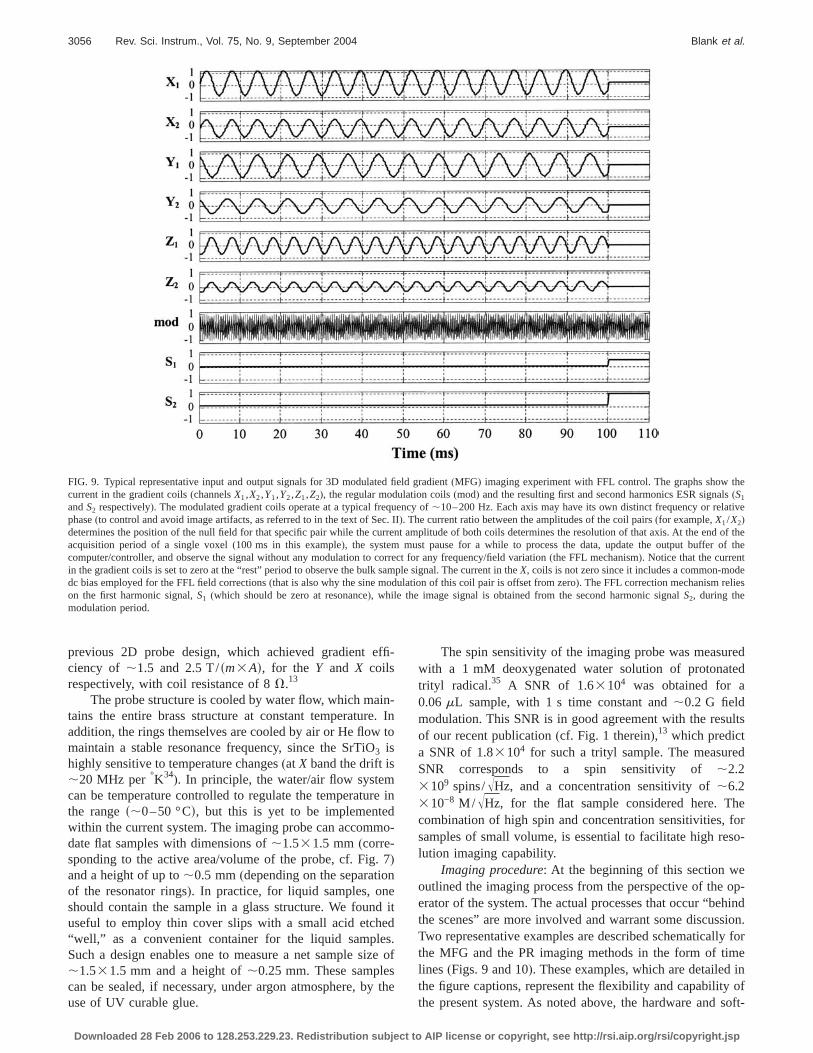
FIG. 9. Typical representative input and output signals for 3D modula current in the gradient coils(channelsX1,X2,Y1,Y2,Z1,Z2), the regular mo andS2 respectively). The modulated gradient coils operate at a typical f phase(to control and avoid image artifacts, as referred to in the text of S determines the position of the null field for that specific pair while the c acquisition period of a single voxel(100 ms in this example), the syste computer/controller, and observe the signal without any modulation to in the gradient coils is set to zero at the “rest” period to observe the bul dc bias employed for the FFL field corrections(that is also why the sine m on the first harmonic signal,S1 (which should be zero at resonance), whil modulation period.
use of UV curable glue.
In
n
t
of
he
The spin sensitivity of the imaging probe was meas with a 1 mM deoxygenated water solution of protona trityl radical.35 A SNR of 1.63104 was obtained for 0.06mL sample, with 1 s time constant and,0.2 G field modulation. This SNR is in good agreement with the res of our recent publication(cf. Fig. 1 therein),13 which predic a SNR of 1.83104 for such a trityl sample. The measu SNR corresponds to a spin sensitivity of,2.2 3109 spins/ÎHz, and a concentration sensitivity of,6.2 310−8 M/ ÎHz, for the flat sample considered here. combination of high spin and concentration sensitivities samples of small volume, is essential to facilitate high r lution imaging capability.
Imaging procedure: At the beginning of this section outlined the imaging process from the perspective of the erator of the system. The actual processes that occur “b the scenes” are more involved and warrant some discus Two representative examples are described schematica the MFG and the PR imaging methods in the form of t lines (Figs. 9 and 10). These examples, which are detail the figure captions, represent the flexibility and capabilit
eld gradient(MFG) imaging experiment with FFL control. The graphs show tion coils(mod) and the resulting first and second harmonics ESR signa(S1
ency of,10–200 Hz. Each axis may have its own distinct frequency or rel IIe current ratio between the amplitudes of the coil pairs(for example,X1/X2) t amplitude of both coils determines the resolution of that axis. At the
ust pause for a while to process the data, update the output buffe ect for any frequency/field variation(the FFL mechanism). Notice that the curren
ple signal. The current in theX, coils is not zero since it includes a common-m tion of this coil pair is offset from zero). The FFL correction mechanism rel image signal is obtained from the second harmonic signalS2, during the
ted fi dula requ ec.). Th urren m m corr
k sam odula e the
the present system. As noted above, the hardware and soft-
oils r l im-
d a
ou y on i is
- at
t -
d -
per nic nic
hich of at is ) e ab- in sults pre- ative ts are
de-
ges
s
the
nals
per- scan n is ob- the nals de
ware support any arbitrary excitation of the gradient c (within the bandwidth of up to,10 kHz). Thus, furthe progress in the direction of, for example, spectral-spatia aging or 3D projection reconstruction may be pursued in future with just software updates.
IV. EXPERIMENTAL RESULTS AND DISCUSSION
We now describe and discuss some representativ perimental results of images acquired with the microsc system. These experiments, performed with solid and li samples, enable us to quantify the resolution, SNR, and age quality obtained in 2D and 3D measurements with MFG and the PR methods. Imaging of the same sam with the two methods provides a good basis for compar and discussion about their different advantages and d vantages. Whenever applicable, the experimental resul compared to prior estimations of image SNR and resolu obtained by cw ESR imaging.13,26
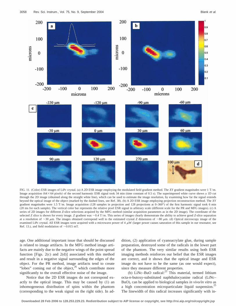
(a) LiPc phantom: As a first example we measure high spin concentration sample of solid LiPc crystal(the same crystal that was measured in our recent publicatio13). Figure 11 provides the measured 2D and 3D images o crystal. The 2D images(Figs. 11(a)and 11(b)), were ac quired with both the PR and the MFG methods. The im SNR (max signal from a voxel divided by the rms of t noise in areas of the image where no radicals are pre) was found to be,110 and,240 for the MFG and PR met ods, respectively. These figures can be compared with theoretical estimates of image SNR,13 and the spin sensitivit of the probe described above. The radical concentrati ,1020 spins in 1 cm336 (provided that the material density ,1), which implies that there are,831011 spins in an im age voxel of 10310380 mm (see below). We know th Q,1000, and the resonator active volume is,3 mm2 (see above)and we also assumeT1 andT2 values similar to tha of 1 mM trityl radical in water solution.13 All these param
-
-
s
- re
s
t
r
s
method[employing Eq.(5) in our recent publication,13 and considering the second harmonic signal]. The PR metho devotes longer acquisition time to each pixel(128 projec tions with sampling time of 20 ms as compared to 0.5 s pixel in the MFG).26 It also uses the stronger first harmo signal (,two times larger than the second harmo signal14), to simplify the de-convolution process.26 These two factors should provide a SNR of the PR method, w is ,4.4f=23 s12830.02/0.5d1/2g times larger than that the MFG method. In practice we obtained a PR SNR th 2.2 times larger, probably due to image artifacts(see below that contribute to the PR image apparent noise. Accurat solute predictions of the image SNR(and the ESR signal general)are somewhat problematic and the present re provide relatively good agreement with the theoretical dictions, both for the absolute SNR values, and the rel SNR between MFG and PR methods. These SNR resul also compatible with the measured probe spin sensitivity scribed in the previous section.
In terms of image resolution, analyzing the ESR ima by taking a 1D cut at certain locations13,37 [Fig. 11(a)] re- veals that the resolution is,10310 mm for the 2D image acquired with both methods, and,30 mm for the z slice separation in the 3D images(the latter number is less reliab due to the difficulty of accurately measuring the crystaZ dimension, which is estimated to be,80 mm).38 The theo retical resolution of the MFG method for 2D imaging w discussed above(cf. Fig. 1). The image in Fig. 11(a)involves gradients of 1 T/m, radical linewidth of 0.01 mT, and m modulation field of 0.015 mT, which results in the calcula 2D resolution of 9.5mm (for the second harmonic signa). The PR method, which observes the first derivative sig requires gradients that are about two times stronger to o a similar resolution.26,39 In the present case, we obtained the PR image a similar resolutions10 mmd to that of the MFG method with gradients of just 1.5 T/m, thanks to
26
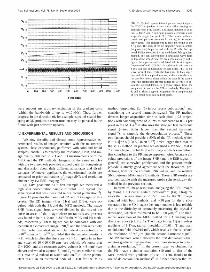
FIG. 10. Typical representative input and output sig for 2D/3D projection reconstruction(PR) imaging experiment with FFL control. The signal notation is as Fig. 9. TheX andY coil pairs provide a gradient alon a specific anglestanf=Y1/X1d. The current within certain coil pair(for exampleX1 andX2) is not neces sarily equal. This enables one to shift the origin in XY plane. The scan of the dc magnetic field(to obtain the projection) is performed with theZ coils. For op tional Z-slice selection by the modulated field grad method, one can superimpose a sinusoidal wave on top of the scanZ field, (as seen schematically in th figure, the superimposed modulated field is at a typ frequency of,10–200 Hz). In addition, in this case t Z coil pair also compensates for field drifts(FFL) so the wave form of these coils also has some dc bias su imposed. As in the previous case, at the end of the (or possibly several times within the scan, if the sca long) the acquisition process pauses for a while to tain the un-modulated/zero gradient signal from sample and to correct the FFL accordingly. The sig S1 andS2 show a typical projection for a sample ma of two small point-like radical grains.
use of de-convolution methodsto further sharpen the im-
sse arti- read d f th eate e
ex-
tom
e n e r, see
age. One additional important issue that should be discu is related to image artifacts. In the MFG method image facts are mainly due to the negative wings of the point sp function [Figs. 2(c) and 2(d)]associated with this metho and result in a negative signal surrounding the edges o object. For the PR method, image artifacts tend to cr “lobes” coming out of the object,26 which contribute mor significantly to the overall effective noise of the image.
Notice that the 2D ESR images do not correspond actly to the optical image. This may be caused by(1) an inhomogeneous distribution of spins within the phan
FIG. 11. (Color) ESR images of LiPc crystal.(a)A 2D ESR image employ Image acquisitions64364 pixelsdof the second harmonic ESR signal to through the 2D image(obtained along the straight white line), which can b beyond the optical image of the object(marked by the dashed lines, see gradient magnitudes were 1.5 T/m. Image acquisition(128 samples in p (20 ms for each sample). The vertical color bar represents the relative p series of 2D images for differentZ-slice selections acquired by the MFG selectedZ slice is shown for every image.Z gradient was,0.4 T/m. This at a resolution of,30 mm. The images obtained correspond well to th examined LiPc crystal. All ESR images were acquired with a microwa Ref. 13.), and field modulation of,0.015 mT.
(corresponding to the weak signal on the right side). In ad-
d
e
dition, (2) application of cyanoacrylate glue, during sam preparation, destroyed some of the radicals in the lower of the phantom. The very similar results using both E imaging methods reinforces our belief that the ESR im are correct, and it shows that the optical image and image do not have to be the same(as one would expec since they measure different properties.
(b) LiNc–BuO radical:25 This material, termed lithium octa-n-butoxy-substituted naphthalocyanine radical(LiNc– BuO), can be applied to biological samplesin vivo/in vitro as a high concentration microparticulate liquid suspensio25
e modulated field gradient method. TheXY gradient magnitudes were 1 T/ 4 min(time constant of 0.5 s). The superimposed white curve shows a 1D
ed to estimate the image resolution, by examining how far the signal 38(b) A 2D ESR image employing projection reconstruction method. ThXY tion and 128 projections at 0–360°) of the first harmonic signal took 6 m SR signal in arbitrary scale(different scale for the PR and MFG images). (c) A hod(similar acquisition parameters as in the 2D image). The coordinate of th s of images clearly demonstrate the ability to achieve goodZ-slice separatio timated crystalZ dimension of,80 mm. (d) Optical microscopy image of th wer of 4mW (larger power causes saturation of this sample in our resonato
ing th ok 3 e us Ref.). rojec ixel E met
serie e es
an s, o orm UV
o e high , lase
. The
voxel ical spot
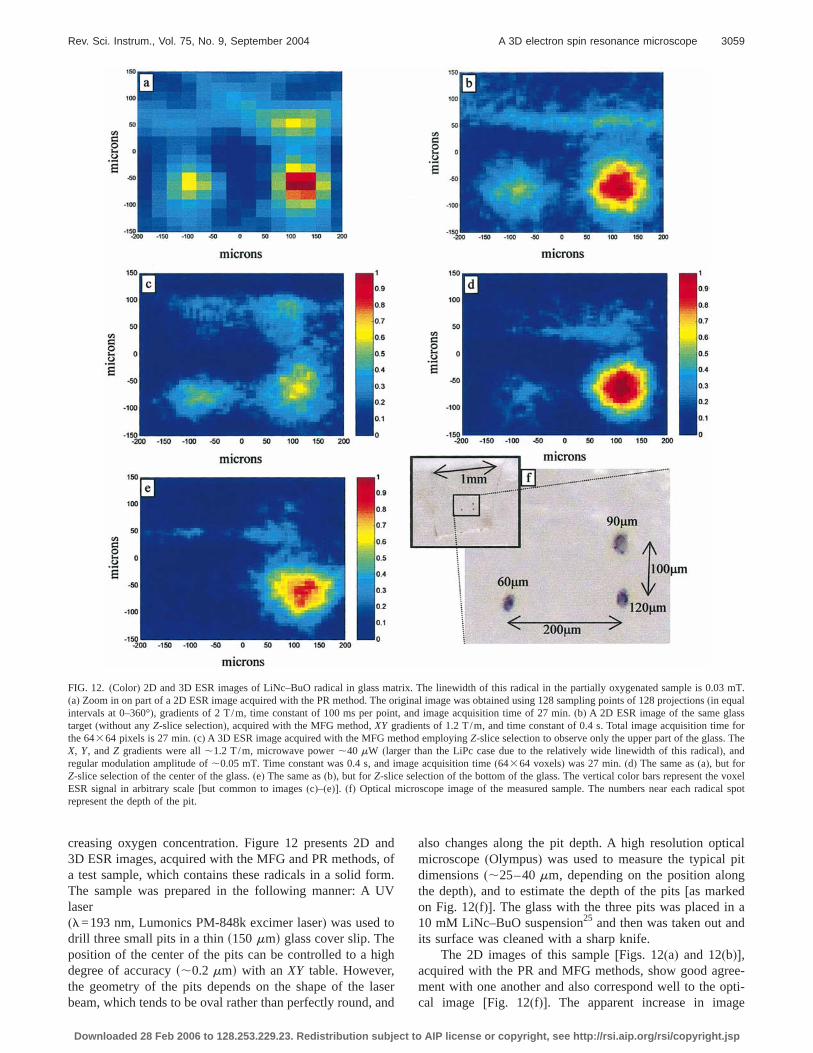
creasing oxygen concentration. Figure 12 presents 2D 3D ESR images, acquired with the MFG and PR method a test sample, which contains these radicals in a solid f The sample was prepared in the following manner: A laser (l=193 nm, Lumonics PM-848k excimer laser) was used t drill three small pits in a thins150 mmd glass cover slip. Th position of the center of the pits can be controlled to a degree of accuracys,0.2 mmd with an XY table. However the geometry of the pits depends on the shape of the
FIG. 12. (Color) 2D and 3D ESR images of LiNc–BuO radical in glass (a) Zoom in on part of a 2D ESR image acquired with the PR method. T intervals at 0–360°), gradients of 2 T/m, time constant of 100 ms per p target(without anyZ-slice selection), acquired with the MFG method,XY g the 64364 pixels is 27 min.(c) A 3D ESR image acquired with the MFG X, Y, and Zgradients were all,1.2 T/m, microwave power,40 mW (lar regular modulation amplitude of,0.05 mT. Time constant was 0.4 s, an Z-slice selection of the center of the glass.(e) The same as(b), but forZ-slic ESR signal in arbitrary scale[but common to images(c)–(e)]. (f) Optical represent the depth of the pit.
beam, which tends to be oval rather than perfectly round, an
d f .
r
also changes along the pit depth. A high resolution op microscope(Olympus)was used to measure the typical dimensions(,25–40mm, depending on the position alo the depth), and to estimate the depth of the pits[as marked on Fig. 12(f)]. The glass with the three pits was placed 10 mM LiNc–BuO suspension25 and then was taken out a its surface was cleaned with a sharp knife.
The 2D images of this sample[Figs. 12(a)and 12(b)] acquired with the PR and MFG methods, show good ag ment with one another and also correspond well to the
ix. The linewidth of this radical in the partially oxygenated sample is 0 riginal image was obtained using 128 sampling points of 128 projectio(in equa and image acquisition time of 27 min.(b) A 2D ESR image of the same gla nts of 1.2 T/m, and time constant of 0.4 s. Total image acquisition tim od employingZ-slice selection to observe only the upper part of the glass
han the LiPc case due to the relatively wide linewidth of this radical), and age acquisition time(64364 voxels)was 27 min.(d) The same as(a), but for lection of the bottom of the glass. The vertical color bars represent the scope image of the measured sample. The numbers near each rad
matr he o oint, radie meth ger t d im e se micro
dcal image [Fig. 12(f)]. The apparent increase in image
t on D 2D
age
with PR
presents the
“noise” [as compared to the 3D images in Figs. 12(c)–12(e)] is probably due to the signal from residual radicals lef both sides of the glass(that are largely eliminated in the 3 image). One important issue that is evident from these images is that the PR image has fewer pixels than the image. This is due to the fact that in the PR method one to acquire information from the entire sample and ca collect information from only a small part of the sample(as the MFG can). In the present case, there were residua nals from the glass surface and the edges of the glass. signals had to be collected with the PR method, which sulted in a rather large image of,232 mm, with only 90 390 pixels (after inverse Radon transform of the 128 p jections, each with 128 samples26). This is a disadvantage f PR in microscopy applications. The 3D ESR image of upper side of the glass[Fig. 12(c)]follows the optical imag closely, but with an additional small signal that is proba due to some residual radicals that were not removed from
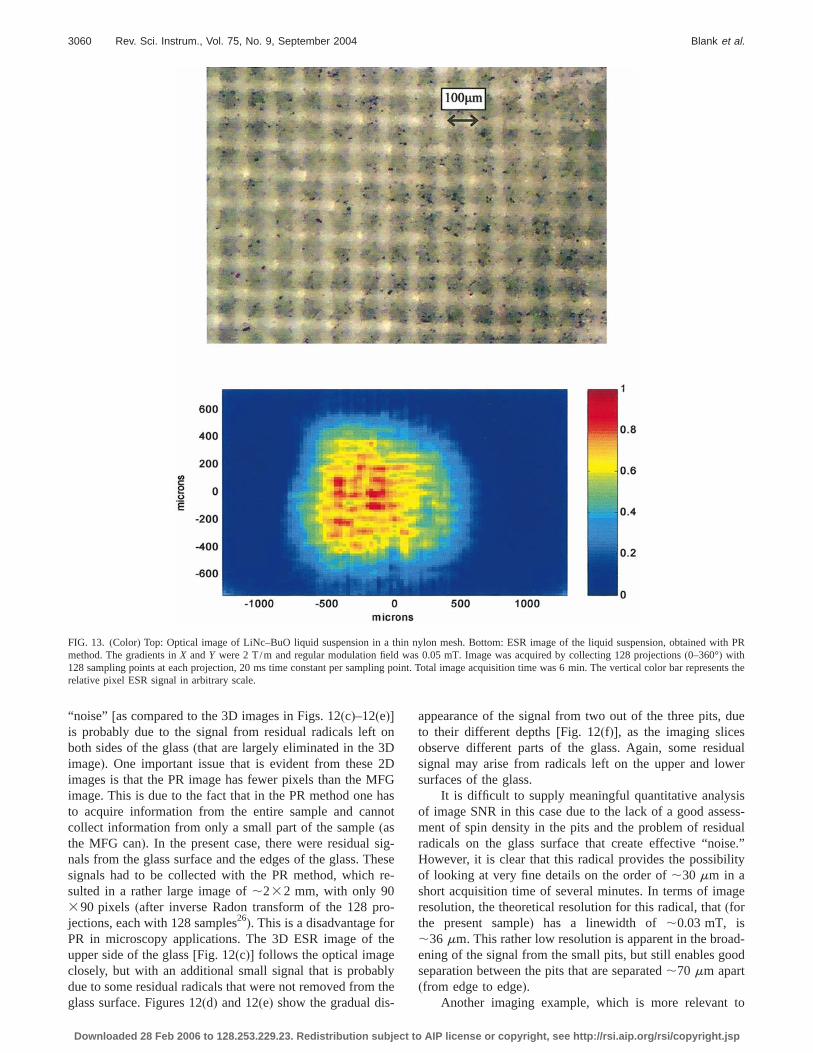
FIG. 13. (Color) Top: Optical image of LiNc–BuO liquid suspension in method. The gradients inX andY were 2 T/m and regular modulation fi 128 sampling points at each projection, 20 ms time constant per samp relative pixel ESR signal in arbitrary scale.
glass surface. Figures 12(d) and 12(e)show the gradual dis-
s
- se
e
appearance of the signal from two out of the three pits, to their different depths[Fig. 12(f)], as the imaging slice observe different parts of the glass. Again, some res signal may arise from radicals left on the upper and lo surfaces of the glass.
It is difficult to supply meaningful quantitative analy of image SNR in this case due to the lack of a good as ment of spin density in the pits and the problem of resi radicals on the glass surface that create effective “no However, it is clear that this radical provides the possib of looking at very fine details on the order of,30 mm in a short acquisition time of several minutes. In terms of im resolution, the theoretical resolution for this radical, that(for the present sample)has a linewidth of ,0.03 mT, is ,36 mm. This rather low resolution is apparent in the bro ening of the signal from the small pits, but still enables g separation between the pits that are separated,70 mm apar (from edge to edge).
n nylon mesh. Bottom: ESR image of the liquid suspension, obtained as 0.05 mT. Image was acquired by collecting 128 projections(0–360°)with oint. Total image acquisition time was 6 min. The vertical color bar re
a thi eld w ling p
Another imaging example, which is more relevant to
the R sio
from two n the - w to anding MR ize, how
mined
biological applications, involves a liquid suspension of same LiNc–BuO radical.25 Figure 13 shows the 2D ES image obtained with the PR method for such a suspen (10 mM concentration)embedded within a fine nylon me (obtained from Goodfellow; mesh aperture 50mm, and wire size 39mm). The PR is the method of choice when o requires fast imaging of the entire sample in order to ob for example, morphological information. Following the quisition of the PR image one can optionally observe in m detail some specific voxels within the sample(employing the MFG). The ESR image clearly shows:(1) the separation o the compartments in the mesh, and(2) that the signal i obtained only from the active area of the resonator(cf. Fig. 7). An interesting point that should be noted is that s radical suspensions are usually employed inin vivo imaging studies with,1 mm resolution, and in this scale the susp sion is rather uniform. However, at the 10mm scale, the suspension is not uniform and some of the areas co larger grains than other areas(as can also be seen in t optical image). This nonuniformity is manifested in the E microimage.
ACKNOWLEDGMENTS
The authors thank Professor P. Kuppusamy, Dr. N. P nandi, and Dr. Y. Deng from the Biomedical EPR Imag Center at Ohio State University for supplying them w samples of the LiNc–BuO radical suspensions and the convolution routine for the PR imaging. This research supported by grants from NIH/NCRR and NSF chemistr
1B. Blumich, NMR Imaging of Materials. Monographs on the Physics Chemistry of Materials(Oxford University Press, Oxford, 2000).
2E. Fukushima,NMR in Biomedicine: The Physical Basis. Key Paper Physics; No. 2.(American Institute of Physics, New York, 1989).
3D. G. Gadian,NMR and its Applications to Living Systems, 2nd ed.(Ox- ford University Press, Oxford, 1995).
4G. R. Eaton and S. S. Eaton, Concepts Magn. Reson.7, 49 (1995). 5G. L. He, A. Samouilov, P. Kuppusamy, and J. L. Zweier, Mol. C Biochem. 234, 359 (2002).
6H. M. Swartz and R. B. Clarkson, Phys. Med. Biol.43, 1957(1998). 7K. I. Yamada, R. Murugesan, N. Devasahayam, J. A. Cook, J. B. Mitc S. Subramanian, and M. C. Krishna, J. Magn. Reson.154, 287(2002).
8P. T. Callaghan,Principles of Nuclear Magnetic Resonance Microsc (Oxford University Press, Oxford, 1991).
9M. Ikeya, Annu. Rev. Mater. Sci.21, 45 (1991). 10F. Sakran, A. Copty, M. Golosovsky, N. Bontemps, D. Davidov, an
Frenkel, Appl. Phys. Lett.82, 1479(2003). 11Z. Xiang and Y. Xu, Appl. Magn. Reson.12, 69 (1997). 12A. Feintuch, G. Alexandrowicz, T. Tashma, Y. Boasson, A. Grayev
and N. Kaplan, J. Magn. Reson.142, 82 (2000).
n
-
-
13A. Blank, C. R. Dunnam, P. P. Borbat, and J. H. Freed, J. Magn. R 165, 116 (2003).
14C. P. Poole,Electron Spin Resonance: A Comprehensive Treatise O perimental Techniques, 2nd ed.(Wiley, New York, 1983).
15J. P. Hornak, J. K. Moscicki, D. J. Schneider, and J. H. Freed, J. C Phys. 84, 3387(1986).
16J. K. Moscicki, Y. K. Shin, and J. H. Freed, J. Magn. Reson.(1969-1992 84, 554(1989).
17S. Gravina and D. G. Cory, J. Magn. Reson., Ser. B104, 53 (1994). 18A. Feintuch, T. Tashma, A. Grayevsky, J. Gmeiner, E. Dormann, an
Kaplan, J. Magn. Reson.157, 69 (2002). 19A. Blank, E. Stavitski, H. Levanon, and F. Gubaydullin, Rev. Sci. Inst
74, 2853(2003). 20P. P. Borbat, A. J. Costa-Filho, K. A. Earle, J. K. Moscicki, and J
Freed, Science291, 266(2001). 21J. H. Freed, Annu. Rev. Phys. Chem.51, 655(2000). 22T. Herrling, N. Klimes, W. Karthe, U. Ewert, and B. Ebert, J. Ma
Reson.(1969-1992)49, 203 (1982). 23T. Herrling, J. Fuchs, and N. Groth, J. Magn. Reson.154, 6 (2002). 24K. Ohno and M. Watanabe, J. Magn. Reson.143, 274 (2000). 25R. P. Pandian, N. L. Parinandi, G. Ilangovan, J. L. Zweier, and P.
pusamy, Free Radic Biol. Med.35, 1138(2003). 26G. R. Eaton, S. S. Eaton, and K. Ohno,EPR Imaging and In Vivo EP
(CRC, Boca Raton, FL, 1991). 27U. Ewert and T. Herrling, J. Magn. Reson.(1969-1992)61, 11 (1985). 28A. J. denDekker and A. vandenBos, J. Opt. Soc. Am. A14, 547 (1997) 29O. Gonen and H. Levanon, J. Phys. Chem.88, 4223(1984). 30J. S. Hyde, H. S. Mchaourab, T. G. Camenisch, J. J. Ratke, R. W. Co
W. Froncisz, Rev. Sci. Instrum.69, 2622(1998). 31A. D. Poularikas,The Transforms and Applications Handbook, 2nd ed
(CRC, Boca Raton, FL, 2000). 32M. Jaworski, A. Sienkiewicz, and C. P. Scholes, J. Magn. Reson.124, 87
(1997). 33J.-M. Jin, Electromagnetic Analysis and Design in Magnetic Reson
Imaging (CRC, Boca Raton, FL, 1999). 34J. Krupka, R. G. Geyer, M. Kuhn, and J. H. Hinken, IEEE Trans. Mi
wave Theory Tech.42, 1886(1994). 35J. H. Ardenkjaer-Larsen, I. Laursen, I. Leunbach, G. Ehnholm, L. G. W
rand, J. S. Petersson, and K. Golman, J. Magn. Reson.133, 1 (1998). 36K. J. Liu, P. Gast, M. Moussavi, S. W. Norby, N. Vahidi, T. Walczak,
Wu, and H. M. Swartz, Proc. Natl. Acad. Sci. U.S.A.90, 5438–544 (1993).
37L. Ciobanu, D. A. Seeber, and C. H. Pennington, J. Magn. Reson.158, 178 (2002).
38Determining the resolution in magnetic resonance microscopy is far trivial. Ideally one would like to look at a test sample consisting of infinitely small points and to determine the minimal distance betwee points that can still be resolved(i.e., the resolution). In practice, in con trast to optical methods, the signal of point-like sample will be too lo be detectable, and the actual fabrication of such a sample is a dem task in itself. Instead, we follow here the conventional approach of N microscopy(Ref. 37), which observes objects of well defined finite s where one may estimate the resolution in the image by measuring sharp is the falloff of the signal at the sample edges, which are deter by the high resolution optical image of the same object.
39T. Herrling, K. U. Thiessenhusen, and U. Ewert, J. Magn. Reson.(1969-
1992) 100, 123(1992).