
ABSTRACT
Title of dissertation: SCANNING TUNNELING MICROSCOPYAT MILLIKELVIN TEMPERATURES:DESIGN AND CONSTRUCTION
Mark Avrum Gubrud,Doctor of Philosophy, 2010
Dissertation directed by: Professor J. Robert AndersonDepartment of Physics
This dissertation reports on work toward the realization of a state-of-the-art
scanning tunneling microscopy and spectroscopy facility operating at milliKelvin
temperatures in a dilution refrigerator. Difficulties that have been experienced in
prior efforts in this area are identified. Relevant issues in heat transport and in
the thermalization and electrical filtering of wiring are examined, and results are
applied to the design of the system. The design, installation and characterization
of the pumps, plumbing and mechanical vibration isolation, and the design and
installation of wiring and fabrication and characterization of electrical filters are
described.
SCANNING TUNNELING MICROSCOPY ATMILLIKELVIN TEMPERATURES:DESIGN AND CONSTRUCTION
by
Mark Avrum Gubrud
Dissertation submitted to the Faculty of the Graduate School of theUniversity of Maryland, College Park in partial fulfillment
of the requirements for the degree ofDoctor of Philosophy
2010
Advisory Committee:Professor J. Robert Anderson, Chair/AdvisorDr. Barry BarkerProfessor Theodore L. EinsteinProfessor Bruce E. KaneProfessor John MelngailisProfessor Johnpierre Paglione
Acknowledgments
I am hopeful that the members of my Advisory Committee will accept my
sincere gratitude for their support in my completing this dissertation and graduating
from the PhD program.
I owe special thanks to Prof. J. Robert Anderson for pushing me to finish,
and to Dr. Bruce Kane and the Laboratory for Physical Sciences for support.
The work reported here was done in direct collaboration with Barry Barker,
Michael Dreyer, Anita Roychowdhury, and Dan Sullivan. Notable contributions
were made by J. B. Dottellis and Sudeep Dutta. Nolan Ballew, George Dearstine,
Peter Krusen, and John Sugrue deserve thanks for their work as well.
Without listing more names, I wish to acknowledge the support, help, encour-
agement, collaboration, teaching, and friendship of many, many more persons over
these past (too many) years.
ii
Table of Contents
List of Tables v
List of Figures vii
1 Introduction 1
1.1 Overview . . . . . . . . . . . . . . . . . . . . . . . . . . . . . . . . . . 1
1.2 A note on units and symbols . . . . . . . . . . . . . . . . . . . . . . . 3
2 Scanning Tunneling Microscopy 5
2.1 Seeing atoms . . . . . . . . . . . . . . . . . . . . . . . . . . . . . . . 5
2.2 Invention of STM . . . . . . . . . . . . . . . . . . . . . . . . . . . . . 9
3 MilliKelvin technology 21
3.1 Thermal conductivity of materials . . . . . . . . . . . . . . . . . . . . 21
3.1.1 Normal metals . . . . . . . . . . . . . . . . . . . . . . . . . . 23
3.1.2 Insulators . . . . . . . . . . . . . . . . . . . . . . . . . . . . . 26
3.2 Thermal contact . . . . . . . . . . . . . . . . . . . . . . . . . . . . . 29
3.2.1 Kapitza resistance: Theory . . . . . . . . . . . . . . . . . . . . 32
3.2.2 Thermal contact resistance: Reality . . . . . . . . . . . . . . . 39
3.2.3 Estimation of thermal boundary resistance: Empirical data . . 43
3.2.4 Comparison of contact and volume thermal resistance . . . . . 44
3.3 Heat leaks . . . . . . . . . . . . . . . . . . . . . . . . . . . . . . . . . 50
3.3.1 Gas conduction . . . . . . . . . . . . . . . . . . . . . . . . . . 51
3.3.2 Radiation . . . . . . . . . . . . . . . . . . . . . . . . . . . . . 55
3.3.3 Geometrical factors . . . . . . . . . . . . . . . . . . . . . . . . 56
3.3.4 Shields . . . . . . . . . . . . . . . . . . . . . . . . . . . . . . . 58
3.3.5 Example calculation: Heat transfer to 50 mK shield . . . . . . 59
3.3.6 Eddy current heating . . . . . . . . . . . . . . . . . . . . . . . 61
3.4 Electrical noise and filtering . . . . . . . . . . . . . . . . . . . . . . . 63
3.4.1 Dissipative dielectric filters . . . . . . . . . . . . . . . . . . . . 64
3.4.2 Dissipative conductor (distributed RC) filters . . . . . . . . . 72
3.5 Thermalization of wiring . . . . . . . . . . . . . . . . . . . . . . . . . 78
3.5.1 Thermalization of a coaxial cable . . . . . . . . . . . . . . . . 78
3.5.2 Thermalization of an unshielded wire . . . . . . . . . . . . . . 84
3.5.3 Thermalization of CuNi and Cu microcoax . . . . . . . . . . . 85
3.5.4 Thermalization of Thermocoax . . . . . . . . . . . . . . . . . 91
3.5.5 Appendix to Sec. 3.5.4: Another method of estimating κp forMgO . . . . . . . . . . . . . . . . . . . . . . . . . . . . . . . . 95
3.5.6 Thermalization of unshielded wiring . . . . . . . . . . . . . . . 99
iii
4 Installation of cryostat, dilution refrigerator, pumps and plumbing 1034.1 Basic facilities . . . . . . . . . . . . . . . . . . . . . . . . . . . . . . . 1034.2 Pit scaffolding . . . . . . . . . . . . . . . . . . . . . . . . . . . . . . . 1054.3 Table installation . . . . . . . . . . . . . . . . . . . . . . . . . . . . . 1084.4 Force on magnet dewar . . . . . . . . . . . . . . . . . . . . . . . . . . 1094.5 Raising and lowering the dewar . . . . . . . . . . . . . . . . . . . . . 1154.6 Initial testing of dilution refrigerator . . . . . . . . . . . . . . . . . . 1184.7 The Vibration Problem . . . . . . . . . . . . . . . . . . . . . . . . . . 1194.8 Pump Room setup . . . . . . . . . . . . . . . . . . . . . . . . . . . . 124
4.8.1 Design . . . . . . . . . . . . . . . . . . . . . . . . . . . . . . . 1244.8.2 Realization . . . . . . . . . . . . . . . . . . . . . . . . . . . . 129
4.9 Sandbox and Dilution Refrigerator Control Panel . . . . . . . . . . . 1334.9.1 Design . . . . . . . . . . . . . . . . . . . . . . . . . . . . . . . 1334.9.2 Realization . . . . . . . . . . . . . . . . . . . . . . . . . . . . 135
4.10 Vibration-Isolated Plumbing to Tabletop . . . . . . . . . . . . . . . . 1414.10.1 Design . . . . . . . . . . . . . . . . . . . . . . . . . . . . . . . 1414.10.2 Realization . . . . . . . . . . . . . . . . . . . . . . . . . . . . 147
4.11 Overall performance . . . . . . . . . . . . . . . . . . . . . . . . . . . 1524.12 Conclusions . . . . . . . . . . . . . . . . . . . . . . . . . . . . . . . . 156
5 Mounting the STM and Wiring the Cryostat 1595.1 STM mount . . . . . . . . . . . . . . . . . . . . . . . . . . . . . . . . 1595.2 Cryostat wiring . . . . . . . . . . . . . . . . . . . . . . . . . . . . . . 164
5.2.1 General requirements . . . . . . . . . . . . . . . . . . . . . . . 1645.2.2 Signal wires . . . . . . . . . . . . . . . . . . . . . . . . . . . . 1665.2.3 Piezo and thermometry wires . . . . . . . . . . . . . . . . . . 1715.2.4 Cold end wiring . . . . . . . . . . . . . . . . . . . . . . . . . . 1755.2.5 Bronze powder filters . . . . . . . . . . . . . . . . . . . . . . . 1775.2.6 Thermocoax filters . . . . . . . . . . . . . . . . . . . . . . . . 186
5.3 Magnetically shielded sample stage for SQUID experiment . . . . . . 1945.4 Conclusions . . . . . . . . . . . . . . . . . . . . . . . . . . . . . . . . 201
6 Conclusions and Further Work 2056.1 Conclusions from the work done so far . . . . . . . . . . . . . . . . . 2056.2 Further work . . . . . . . . . . . . . . . . . . . . . . . . . . . . . . . 208
Bibliography 210
iv
List of Tables
3.1 Thermal conductivity data for selected normal metals . . . . . . . . . 27
3.2 Thermal conductivity data for selected amorphous insulators . . . . . 29
3.3 Some thermal boundary resistivity data for deposited contacts . . . . 44
3.4 Selected thermal boundary resistance data for pressed contacts . . . . 44
3.5 Vapor pressure and mean free path of 4He and 3He . . . . . . . . . . 53
3.6 Thermal conductivity data for estimating that of powdered MgO . . . 96
3.7 Estimated thermalization lengths for unshielded wire varnished to Cuposts . . . . . . . . . . . . . . . . . . . . . . . . . . . . . . . . . . . . 102
4.1 Summary of vibration measurements taken at the tabletop . . . . . . 157
5.1 Wires needed for the dual mK-STM system . . . . . . . . . . . . . . 165
5.2 Wires provided for the dual mK-STM system . . . . . . . . . . . . . 202
v
List of Figures
2.1 Field electron/ion microscopy . . . . . . . . . . . . . . . . . . . . . . 8
2.2 Field emission and MVM tunneling . . . . . . . . . . . . . . . . . . . 13
2.3 STM scanner and walker design . . . . . . . . . . . . . . . . . . . . . 16
3.1 Metal powder filters . . . . . . . . . . . . . . . . . . . . . . . . . . . . 69
3.2 Distributed RC filters . . . . . . . . . . . . . . . . . . . . . . . . . . . 73
3.3 Thermalization of a coaxial cable . . . . . . . . . . . . . . . . . . . . 79
3.4 MgO powder in Thermocoax . . . . . . . . . . . . . . . . . . . . . . . 93
4.1 Pit and platform . . . . . . . . . . . . . . . . . . . . . . . . . . . . . 107
4.2 Estimation of force on magnet dewar . . . . . . . . . . . . . . . . . . 111
4.3 Winch . . . . . . . . . . . . . . . . . . . . . . . . . . . . . . . . . . . 117
4.4 Plan of plumbing and vibration suppression . . . . . . . . . . . . . . 121
4.5 Vibration measured at the tabletop . . . . . . . . . . . . . . . . . . . 123
4.6 Vibration of tabletop due to pumps . . . . . . . . . . . . . . . . . . . 127
4.7 Installation of pumps in pump room . . . . . . . . . . . . . . . . . . 131
4.8 Sandbox front and back . . . . . . . . . . . . . . . . . . . . . . . . . 137
4.9 Sandbox right and left . . . . . . . . . . . . . . . . . . . . . . . . . . 139
4.10 Pumps and plumbing isolation principles . . . . . . . . . . . . . . . . 146
4.11 Tabletop plumbing . . . . . . . . . . . . . . . . . . . . . . . . . . . . 149
4.12 Bellows box . . . . . . . . . . . . . . . . . . . . . . . . . . . . . . . . 150
4.13 Performance of the table without plumbing . . . . . . . . . . . . . . . 153
4.14 Vibration compared with Davis lab . . . . . . . . . . . . . . . . . . . 155
5.1 STM mount . . . . . . . . . . . . . . . . . . . . . . . . . . . . . . . . 161
vi
5.2 STM signal wiring schemes . . . . . . . . . . . . . . . . . . . . . . . . 167
5.3 Wiring and thermal anchoring in IVC . . . . . . . . . . . . . . . . . . 172
5.4 Metal powder filter with 4 lines . . . . . . . . . . . . . . . . . . . . . 178
5.5 Making of powder filters . . . . . . . . . . . . . . . . . . . . . . . . . 180
5.6 Powder filter construction . . . . . . . . . . . . . . . . . . . . . . . . 183
5.7 Thermocoax filter rack . . . . . . . . . . . . . . . . . . . . . . . . . . 188
5.8 Cutting and connectorizing Thermocoax . . . . . . . . . . . . . . . . 190
5.9 Thermocoax filter spools . . . . . . . . . . . . . . . . . . . . . . . . . 193
5.10 Winding Thermocoax filters . . . . . . . . . . . . . . . . . . . . . . . 195
5.11 Sample stage for SQUID experiment . . . . . . . . . . . . . . . . . . 197
vii
List of Abbreviations
ac Alternating current, or the time-varying componentAMM Acoustic mismatch model of thermal boundary resistanceatm. Atmospheric pressure, 1.01 × 10⁵ PaBCB Benzocyclobutene, a polymer used in a family of negative photoresistsBCS Theory of superconductivity named for its creators, J. Bardeen, L. N.
Cooper, J. R. SchriefferCDW Charge density wave, a state of nonuniform (periodic) charge density,
generally observable in STM below some ordering temperatureCMN Cerium magnesium nitrate, a paramagnetic salt used for thermometryCNC Computer numerically controlled machine tool
dc Direct current, or the constant componentDMM Diffuse mismatch model of thermal boundary resistance
emf Electromotive force, or magnetically induced voltageFEM Field electron microscopyFIM Field ion microscopy
ID Inner diameterIVC Inner vacuum can, the evacuated space of a fridge, where things get coldlbf Pounds force, i.e. 1 pound mass times the acceleration of gravity
LDOS Local density of states, a measure of the number of electron states perinterval of energy, around some given energy, weighted by the overlap ofthose states with some “local” volume
LHe Liquid heliumLN2 Liquid nitrogenLPS Laboratory for Physical Sciences in College Park, Md.
MVM Metal-vacuum-metal tunnelingMXC Mixing chamber, the coldest part of a dilution refrigerator
Pa Pascal (unit of pressure)PID A control system in which the feedback signal is a sum of proportional,
integral and derivative terms of the sensor dataPTFE Polytetrafluoroethylene, the most common type of Teflon
PZT Lead zirconium titanate, a strongly piezoelectric ceramicOD Outer diameter
OVC Outer vacuum can, the vacuum space which insulates the LHe bath fromroom temperature
OFHC Oxygen-free high conductivity, a moderate purity grade of copper metalrf Radio frequency
RRR Residual resistivity ratio, the ratio of resistivity of a normal metal atroom temperature to resistivity very cold
viii

RT Room temperatureSQUID Superconducting quantum interference deviceSS304 AISI 304 stainless steelSTM Scanning tunneling Microscope or MicroscopySTS Scanning tunneling spectroscopy
WKB A method for approximate solution of Schrodinger’s equation, named forits creators, G. Wentzel, H. Kramers, L. Brillouin
ix
Chapter 1
Introduction
1.1 Overview
Experimental work at technological extremes is naturally difficult. Scanning
tunneling microscopy (STM) and spectroscopy (STS) at milliKelvin temperatures
(mK-STM) represents the intersection of several extremes: ultra-low temperatures
(for physical instruments connected to the outside world), atomic resolution imaging,
ultra-low electrical noise and high-gain amplification of low-level signals, ultra-high
vacuum, and ultra-low vibration levels and/or high mechanical stability in a low
temperature compatible instrument. Quantitatively, one seeks to work at temper-
atures around 30 mK, with voltage resolution of ∼10µV, and current signals as
low as 10 pA, under vacuum of 10−11 Pa or better, with tip-sample distance stable
to ∼1 pm. The degree to which one can achieve these conditions simultaneously
will determine the quality of experimental data obtained, and make the difference
between significant findings and incomprehensible noise.
This dissertation reports progress toward realizing a state-of-the-art milliKelvin
STM system at the Laboratory for Physical Sciences in College Park, MD. At the
time of writing, the system is not yet operational, but the required “physical plant”
infrastructure has been substantially completed. Initial testing, using an STM head
that has demonstrated atomic resolution at room temperature (RT) is expected to
1
begin within weeks.
In undertaking the design and construction of this sytem, I have been guided
by the experiences of a handful of other groups around the world who have built mK-
STM systems and reported their results. I have also looked in depth at phenomena
of heat transport at milliKelvin (mK) temperatures, and tried to apply what I
have learned. In addition, I have surveyed the available literature on vibration
isolation in STM and low-temperature STM, control of mechanical noise from the
1 K pot in a dilution refrigerator, cryostat wiring and thermal anchoring methods,
and cryogenic low-pass filters. Some of this is reported here, but I do not claim to
present comprehensive surveys.
I begin, in Chapter 2, with a review of the history and basics of STM.
Then, in Chapter 3, I review the basics of milliKelvin technology–how to design
and build apparatus that operates at temperatures well below 1 K. I pay particular
attention to issues of thermal transport, contact and insulation, thermalization of
electrical wiring that connects the mK apparatus and the room temperature envi-
ronment, and I estimate thermal performance parameters for particular materials
and configurations that I used in this system. I also discuss low-pass electrical fil-
ters, an important consideration bearing in mind that 100 mK corresponds to 2
GHz, and that thermal or technological electromagnetic energy can be a significant
source of heating and interference in mK experiments.
In Chapter 4, I describe the physical installation of the dilution refrigerator
for our mK-STM and my design and construction of its vibration-isolated system
of pumps and plumbing. I assess the performance of the vibration isolation system
2
both in the context of what was achievable in this installation and in comparison
with more expensive facilities.
In Chapter 5, I describe and discuss issues related to the installation of an
STM in the dilution refrigerator and my design and construction of an rf-shielded
STM mount, electrical wiring of the cryostat, and two types of cold low-pass filters.
In Chapter 6, I state conclusions drawn from this work, and discuss further
work to be done in completing the mK-STM system, studies we may be able to
conduct with it, and issues related to Josephson phase STM.
1.2 A note on units and symbols
Because this dissertation reports and serves as a reference for experimental
work, I have tried to be as consistent and explicit as possible about units, dimen-
sions, and the meaning of particular symbols. Throughout the text I have used
the logically consistent convention of treating the symbols for dimensioned physical
quantities such as temperature and pressure as representing dimensions multiplied
by numbers, rather than as pure numbers, and of displaying the dimension units
used in the expression when mathematical consistency requires reducing the quan-
tity to a dimensionless number, such as when raising to an arbitrary exponent in a
power law or as the argument of an exponential function. Thus, one will see expres-
sions such as “(T/K)1.3,” meaning “the temperature T (which may be expressed
in any absolute units) divided by 1 K, (the result) raised to the power 1.3.” Other
conventions, such as treating the units as implicit, or canceling fractional exponents
3
elsewhere in an expression, are, I believe, more apt to lead to confusion about the
units used or about the correct interpretation of an expression, or to doubt about
whether it is stated correctly.
While I have preferentially used SI units, expressed in their conventional ab-
breviated forms, in practical work in our lab we specify machine parts in decimal
inches, and we use many commercial components which are specified in whole or
fractional inch units. While I could easily convert the latter to m or mm, it does
not seem a reasonable thing to do, since anyone who uses the information in the
future would need to convert back in order to obtain the useful specification–and
might miss the fact that it is an inch specification. Also, I have sometimes expressed
forces in both lbf and N because the former is familiar to Americans and provides
an intuitive sense of force magnitude.
4
Chapter 2
Scanning Tunneling Microscopy
2.1 Seeing atoms
Atoms are much smaller than the wavelength of visible light, and therefore
can never be imaged by ordinary light microscopy. They are comparable in size to
the wavelength of free electrons with kinetic energies comparable to the potential
that binds electrons within the atoms1, suggesting (but see below) that electron
microscopes able to resolve atoms would destroy them. Thus, although X-ray, elec-
tron and neutron diffraction, nuclear magnetic resonance, and the observations of
chemistry are among the sources of data from which atomic crystal and molecular
structures can be inferred and modeled (which might be called indirect imaging), the
direct, real-space imaging, i.e. microscopy, of individual atoms and atomic lattice
defects was once thought to be extremely difficult, perhaps impossible.
This view began to be challenged as early as the mid-1930s by E. W. Muller’s
development of field electron microscopy (FEM)[14], which exploits the particular
geometry and physics of field emission from a sharp metallic needle (typically tung-
sten). As shown in Fig. 2.1 A, in FEM the tip of the needle (cathode) is placed
behind an extraction anode at around 10 kV potential, inducing an electric field
which could exceed several GV/m at the tip. Since the work function confining
1This follows from Bohr quantization, with the virial theorem.
5
electrons within metals is a few eV, electrons beyond about 1 nm from the tip sur-
face have tunneled past the barrier and can be accelerated away from the tip by the
field. Emission will occur most strongly where the barrier is narrow and low, that
is, where the field is strongest, around surface asperities, and also where the work
function is lowest. Modeling the tip as a hemisphere of 10-100 nm radius, the field
around it is nearly radial and induces a radial acceleration of the emitted electrons,
so that the direction of their radiation away from the tip corresponds to the location
on the tip from which they were emitted. The electrons strike a phosphor screen
(or microchannel plate in later versions), mapping a few µm of the tip to a few cm
of the screen.
A tiny hemisphere cut from a crystal will have flat faces corresponding to the
low-index planes, which show up as dark circles in FEM (Fig. 2.1B) since the field
is weaker above the flat faces than above the rounded and atomically rough surface
between them. In the high field and typical temperatures in FEM of around 1000 K,
atoms slowly desorb from the tip, causing the dark circles in the image to collapse
as successive planes evaporate. By evaporating a low work-function metal such as
barium onto the tip, emission can be enhanced, and as early as 1938 Muller noted
the blurry images of isolated objects, which he interpreted as single adsorbed atoms
[15] (Fig. 2.1 B). The FEM can also image single molecules decorating the tip, and
can even reveal their symmetries (Fig. 2.1 C), but the molecules are not resolved.
Resolution in the FEM is at best 1-2 nm, determined by the length scale of field
emission (higher voltage will give better resolution but at too high a field strength
the tip material will evaporate at too high a rate) as well as the curvature of the
6
field around emitting asperities, and the spread of electron initial velocities parallel
to the surface.
By introducing a low pressure of helium gas and reversing the polarity, Muller
created field ion microscopy (FIM), in which helium ions created by the field are
projected to the screen, instead of electrons. The mechanics are somewhat compli-
cated [16], but the main source of contrast is that ionization occurs most strongly
within small regions of high field directly over atomic-scale asperities. By the mid-
1950s, FIM had achieved resolution of 0.3 nm and could provide clear images of the
atomic lattice of an FIM tip. In contrast to FEM, where the tip is often heated to
enhance emission, in FIM the tip is often cryogenically cooled to enhance resolution
and suppress field desorption of the tip atoms.
Although FEM and FIM provided the first direct imaging of atomic-scale
features of a metal surface, and have been useful in the study of defects in metals
[17], their application is limited by the requirement that the sample take the form
of a sharp needle, and by the high field which can desorb surface atoms (Fig. 2.1 D),
limiting the range of materials that can be studied mainly to hard metals. FIM
is also used to examine tips in scanning tunneling microscopy (STM), where FIM
can reveal the tip radius, shape and cleanliness, and field desorption can be used
for further cleaning and smoothing of the apex. This requires that the FIM be
integrated within a UHV STM system.
By the early 1970s, transmission electron microscopes (TEM) were also shown
capable of imaging isolated heavy atoms [20, 21], and high-resolution TEM is today
often used to image the atomic structure of inorganic crystals. The expectation
7
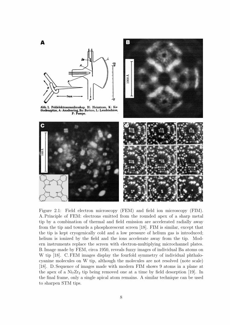
Figure 2.1: Field electron microscopy (FEM) and field ion microscopy (FIM).A. Principle of FEM: electrons emitted from the rounded apex of a sharp metaltip by a combination of thermal and field emission are accelerated radially awayfrom the tip and towards a phosphorescent screen [18]. FIM is similar, except thatthe tip is kept cryogenically cold and a low pressure of helium gas is introduced;helium is ionized by the field and the ions accelerate away from the tip. Mod-ern instruments replace the screen with electron-multiplying microchannel plates.B. Image made by FEM, circa 1950, reveals fuzzy images of individual Ba atoms onW tip [18]. C. FEM images display the fourfold symmetry of individual phthalo-cyanine molecules on W tip, although the molecules are not resolved (note scale)[18]. D. Sequence of images made with modern FIM shows 9 atoms in a plane atthe apex of a Ni7Zr2 tip being removed one at a time by field desorption [19]. Inthe final frame, only a single apical atom remains. A similar technique can be usedto sharpen STM tips.
8
that electrons of sufficiently short wavelength to resolve atoms would be energetic
enough to ionize or dislodge them is correct; in fact electron optics requires energies
of 100 keV and above to achieve atomic resolution. However, the interaction between
one atom and one 100 keV eletron is usually very weak, with a small probability of
a strong (ionizing) interaction. With a very low beam current, a phase contrast
mechanism can be used to image the columns of atoms in ultrathin sections of prop-
erly aligned crystals [22]. Image interpretation can be complicated, and instruments
capable of atomic resolution also have price tags in the $ million range.
2.2 Invention of STM
Like optical microscopy, FEM/FIM and TEM magnify an image by the geo-
metry of projection. Our eyes do something similar, but another way we have to
“see” things is to explore them directly with our hands. This is the principle used
in scanning probe microscopies (SPM), which scan over the surface of the sample
with a local probe having a sufficiently small region of sensitivity. Measurement of
microscopic features by direct mechanical contact of a stylus probe is the principle of
surface profilometers which have been in use for many decades [23]. The surprising
thing is that it is not too hard to make a probe with a “spot size” small enough to
resolve atoms.
The development of scanning tunneling microscopy (STM) during the 1980s
provided a simple and relatively cheap method of imaging atoms, molecules, and
lattices at the surfaces of electrically conducting samples. G. Binnig and H. Rohrer
9
announced STM in 1981 [24], and just 5 years later were awarded the Nobel Prize
for their invention. STM quickly gained widespread use, producing images which
captured headlines and dominated scientific journals, and contributing to the sense
that a new age of nanotechnology was beginning. It turned out that the same
“hands” that can “feel” atoms and molecules can also pick them up, move them
around, and perform other actions at the atomic scale. Less than a decade after
its invention, STM had enabled not only the imaging of a wide range of samples,
but also the precise manipulation of individual atoms [25] and probing of electronic
phenomena at the nanoscale.
STM involves bringing a sufficiently sharp conducting tip sufficiently close to a
nearly flat sample surface that tip and sample electron states overlap, ideally within
a region of atomic proportions. When a voltage (typically ∼1 V or less) is applied
between the tip and sample, a measurable tunneling current (typically 10-1000 pA)
can pass between them. The tunneling current will depend on the tip-sample voltage,
tip-sample distance, and local (atomic-scale) features of the sample and tip electronic
systems where they overlap. These features include information about the locations
and identities of atomic nuclei, but may also reflect purely electronic phenomena,
such as the long-range influence of impurities, trapped charge and defect states,
charge density waves and superconductivity.
To record an image, the tip is raster scanned across the surface by a piezo-
electric scanner capable of repeatable motion at the atomic scale. In the most
common mode of imaging, the tunneling current, at constant voltage, is kept con-
stant by varying the tip height as the tip moves over the sample surface. Even at
10
the considerable standoff distances of ∼0.5 nm typically used in STM, the exponen-
tial dependence of the current on distance is roughly a factor of e per Bohr radius
(∼0.05 nm) [26]. Hence the tip height tracks the sample topography with high verti-
cal resolution, subject to variations in the local density of states (LDOS) at different
points on the sample surface. The images recorded in this way can appear almost
like photographs, although their interpretation can be more problematic.
Ironically, Young et al. had come close to inventing STM more than a decade
earlier, developing an instrument of almost identical schematic design (Fig. 2.2 B)
which they called the Topografiner [27]. However, instead of direct tunneling be-
tween tip and sample at low voltage, they applied a high voltage (∼100 V) between
tip and sample, with a vacuum gap of at least 2 nm, producing field emission from
the tip – as in FEM, but in this case the tip is used as a probe, rather than being
imaged as a sample.
According to the Fowler-Nordheim theory, field emission in the Topografiner
can be understood as the tunneling of electrons from states in the tip to free states
in the vacuum. A crude model is shown in Fig. 2.2 A. The space to the left of the
E (energy) axis, z < 0, represents the tip. The work function U(z) is the energy
required to remove an electron from a state at the Fermi level EF to a distance
z beyond the (nominal) end of the tip; with the vacuum level defined as zero,
U(∞) ≡ −EF . Field emission occurs when the tip is biased at a negative voltage
V relative to the sample plate, located at a distance d from the tip. For electrons
at EF , a classical barrier exists for the region of z > 0 where EF + U(z) > |eV z/d|.
Fig. 2.2 A shows two cases, with V2 > V1 so that the barrier width z2 < z1. A simple
11
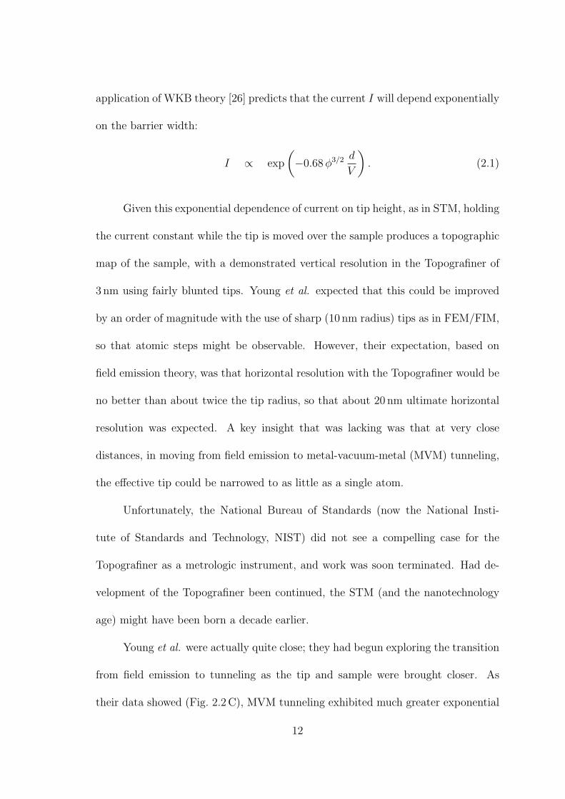
application of WKB theory [26] predicts that the current I will depend exponentially
on the barrier width:
I ∝ exp
(
−0.68 φ3/2 d
V
)
. (2.1)
Given this exponential dependence of current on tip height, as in STM, holding
the current constant while the tip is moved over the sample produces a topographic
map of the sample, with a demonstrated vertical resolution in the Topografiner of
3 nm using fairly blunted tips. Young et al. expected that this could be improved
by an order of magnitude with the use of sharp (10 nm radius) tips as in FEM/FIM,
so that atomic steps might be observable. However, their expectation, based on
field emission theory, was that horizontal resolution with the Topografiner would be
no better than about twice the tip radius, so that about 20 nm ultimate horizontal
resolution was expected. A key insight that was lacking was that at very close
distances, in moving from field emission to metal-vacuum-metal (MVM) tunneling,
the effective tip could be narrowed to as little as a single atom.
Unfortunately, the National Bureau of Standards (now the National Insti-
tute of Standards and Technology, NIST) did not see a compelling case for the
Topografiner as a metrologic instrument, and work was soon terminated. Had de-
velopment of the Topografiner been continued, the STM (and the nanotechnology
age) might have been born a decade earlier.
Young et al. were actually quite close; they had begun exploring the transition
from field emission to tunneling as the tip and sample were brought closer. As
their data showed (Fig. 2.2 C), MVM tunneling exhibited much greater exponential
12
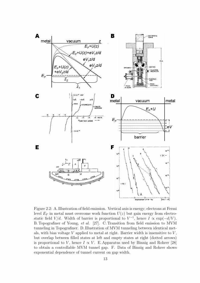
Figure 2.2: A. Illustration of field emission. Vertical axis is energy; electrons at Fermilevel EF in metal must overcome work function U(z) but gain energy from electro-static field V/d. Width of barrier is proportional to V −1, hence I ∝ exp(−d/V ).B. Topografiner of Young, et al. [27]. C. Transition from field emission to MVMtunneling in Topografiner. D. Illustration of MVM tunneling between identical met-als, with bias voltage V applied to metal at right. Barrier width is insensitive to V ,but overlap between filled states at left and empty states at right (dotted arrows)is proportional to V , hence I ∝ V . E. Apparatus used by Binnig and Rohrer [28]to obtain a controllable MVM tunnel gap. F. Data of Binnig and Rohrer showsexponential dependence of tunnel current on gap width.
13
sensitivity to tip height than field emission, with linear rather than exponential
dependence on voltage. While noting this much higher sensitivity, they stated that
“The instrument is never operated in this region due to the instability resulting
from the high gain and because the emitter is only tens of angstroms from the
surface....”[27].
Part of the problem was the electronics; Young et al. used a constant-current
supply which both regulated tip-sample voltage to maintain a set current level, and
generated a correction signal to adjust tip-sample separation. Adapted to the field
emission regime, this control of two physical parameters simultaneously, based on
feedback from a single measurment affected by both parameters, was needlessly
complex and difficult to stabilize in the MVM tunneling regime. In STM, voltage is
usually fixed, and tip-sample distance is controlled by feedback to maintain constant
current. A logarithmic amplifier is usually inserted into the feedback loop to linearize
the exponential dependence of current on distance.
Binnig and Rohrer picked up where Young had left off, using a very simi-
lar piezoelectric positioner to control tip-sample distance to subatomic precision
and measure the exponential dependence of MVM tunneling current on distance
(Fig. 2.2 F) [28]. They went to extraordinary lengths to isolate their apparatus
from environmental vibrations, including the use, later seen to be unecessary, of
magnetic levitation over a superconducting Pb bowl cooled by liquid helium (LHe)
(Fig. 2.2 E). In addition, for coarse approach, bringing tip and sample within tunnel-
ing range, instead of a mechanical screw they used a piezoelectric walker, or “louse,”
a more stable and “hands-free” approach.
14
With the use of three matchstick-like piezoelectric elements to form an XYZ
positioner, and a feedback loop to maintain constant current by controlling the Z
piezo, Binnig and Rohrer’s MVM tunneling device became the first STM [29], and its
further refinement enabled them to obtain clear atomic-resolution images, including
images of the Si(111) surface with its 7×7 reconstruction (Fig. 2.3 A), the first data
by which it was possible to unambiguously determine which of several proposed
structures was correct [30].
Development of the STM proceeded rapidly as more and more groups took
it up. One of the most important early advances was the introduction by Binnig
and Smith [32, 33] of the tube scanner to replace the piezoelectric “matchstick box”
of the original STM. Tube scanners are simpler in construction, and have higher
mechanical resonance frequencies and hence better vibration immunity.
In the usual mode of operation of piezoelectric elements made of ceramics
such as lead zirconium titanate (PZT), an electric field applied in one direction
causes the material to contract in a transverse dimension (Fig. 2.3 B), while reversing
the polarity causes the material to expand in that dimension. Therefore, in the
matchstick-type elements, as used in the Topografiner and in the first STMs, the
electric field is applied transverse to the length of the stick, and the large aspect
ratio serves to multiply the total change in length for a given applied voltage. To
make an XYZ scanner, one such element is provided for each of the 3 directions.
The tube scanner uses a somewhat more clever mechanism (Fig. 2.3 C). A
single electrode coats the inner surface of the tube, the outer surface is divided into
four quadrant electrodes. The voltage applied to the inner electrode, relative to the
15
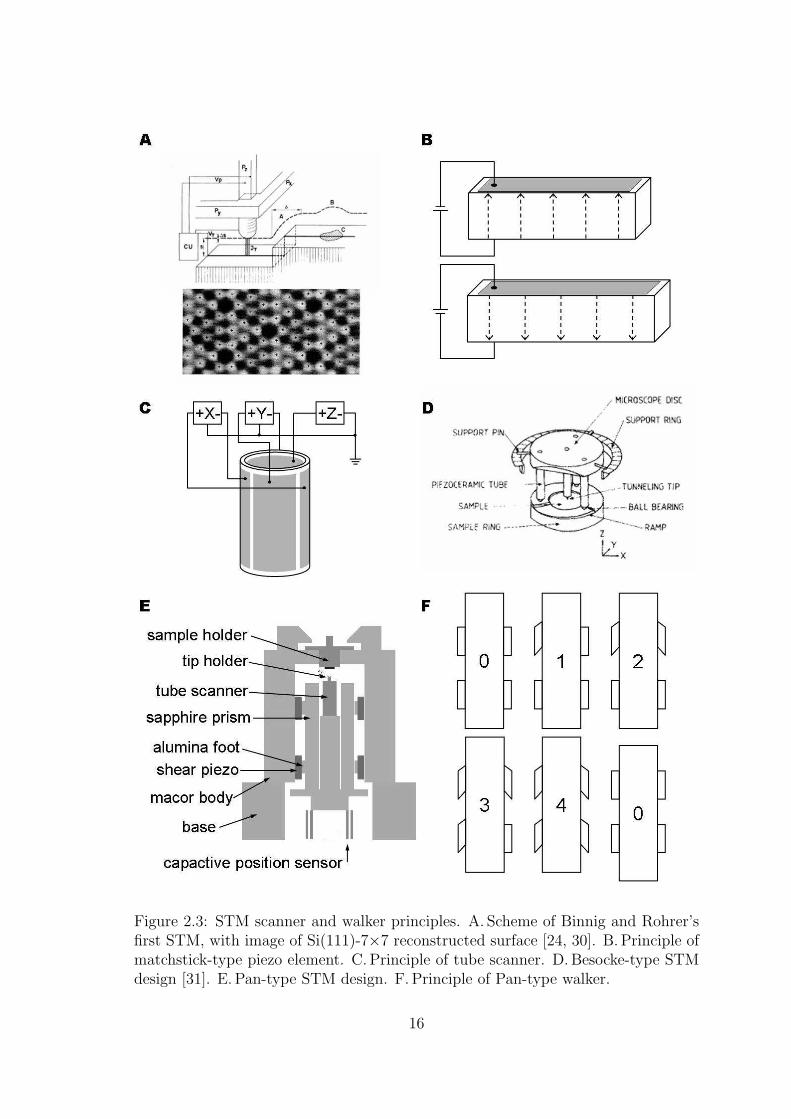
Figure 2.3: STM scanner and walker principles. A. Scheme of Binnig and Rohrer’sfirst STM, with image of Si(111)-7×7 reconstructed surface [24, 30]. B. Principle ofmatchstick-type piezo element. C. Principle of tube scanner. D. Besocke-type STMdesign [31]. E. Pan-type STM design. F. Principle of Pan-type walker.
16
average of voltages applied to the outer electrodes, controls the Z (axial) extension
and contraction of the tube. Bending in the X and Y directions is induced by
differences in the extension/contraction of opposite sides of the tube. Thus the
application of differential voltages to opposing pairs of outer electrodes controls the
XY motion. By referencing all voltages to a common level, e.g. ground, the X, Y,
and Z motions are controlled separately, with only five wires.
Another critical area of development was the coarse approach mechanism.
Tunneling currents can normally be detected only when the tip is within ∼1 nm of
a sample surface, and the tip has to approach this close from a starting distance
of typically several mm, or what can reasonably be arranged by hand and eye.
Moreover, the Z range of piezoelectric scanners is typically ∼1µm. The coarse
approach problem is to bring the tip-sample gap to within this distance. The size of
steps taken during the approach should be smaller than about half the scan range.
The procedure can then be to take a coarse step forward, and with a small tip-
sample voltage applied, ramp the scanner to its full extension while monitoring for
any sign of tunnel current. If there is none, relax the scanner and take another
coarse step forward, repeating until the tip-sample gap is within range and a tunnel
current is detected. If it is known that some hundreds of steps have to be taken
before there is any risk of making contact, this can be done without ramping the
scan piezo each time. However, a tip-sample crash will usually ruin a tip or at least
require its reconditioning by field emission.
The overall geometry of an STM can be considered as constituting a “figure G”,
which represents the tip suspended over the horizontal sample surface and connected
17
to it by the “backbone” loop of the “G.” The size and rigidity of this loop determines
the ability of the STM to control the position of the tip relative to the sample
with a precision of 10–100 pm. A key weakness is the coarse approach mechanism
which must be included within this loop. It is generally less rigid than the other
components of the loop (the scanner, tip and sample holders). Finding a good,
dimensionally stable and rigid mechanism, which repeatably and reliably moves in
steps of the right size, has been a process of trial, error and ingenuity.
The “louse” coarse approach mechanism of the original STM used a piezoelec-
tric plate with three “feet” to “walk” horizontally [29]. The “feet” were metallic
and rested on high-dielectric constant insulators with ground plates underneath.
By applying high voltage to the “feet” they could be selectively clamped and un-
clamped to the insulators by electrostatic force, and by a cycle of clamping, expand-
ing, unclamping, contracting, etc., the “louse” could be walked around in steps of
10–1000 nm.
Other early coarse approach mechanisms included mechanical screws and screw-
driven mechanisms [34, 35] using mechanical leverage and differential bending of
springs to reduce the scale of motion. These crude methods were generally unsat-
isfactory, both because of static friction leading to too-coarse motion, and the need
to turn the screws by hand, often disturbing the tip-sample gap enough to cause
a crash. However, Guha et al. [36] describe a method using a motor-driven screw
with a 20:1 mechanical lever reduction, combined with a piezoelectric array similar
to the Pan design (below). The piezoelectric elements are used not to move the tip
but rather to create vibrations which break static friction. They also provide a rigid
18
grip when inactive.
A simple and ingenious design by Besocke [37, 31] (Fig. 2.3 D), uses a triangle
of three scan tubes to both scan the tip and, for coarse approach, walk up and down
a spiral of ramps. The tubes are mounted on a disk with the tip hanging from the
center, and rest on metal balls which contact the ramp surfaces. Sudden motion of
the tubes causes the balls to slip on the ramps, while with slow motion the balls
stick and the disk moves. The same stick-slip motion can also be used to coarse
position the tip in the XY plane. A variation on this design is to use the Besocke
mechanism for coarse approach only, and use a separate tube scanner for the fine
scanning [38].
Many other designs have made use of the intertial stick-slip mechanism, usually
in linear configurations, both for coarse Z and also XY positioning [39, 40, 41, 42].
Such mechanisms are more successful when used for horizontal XY positioning than
for sample approach, particularly when the latter is done vertically. It is difficult to
precisely counterbalance a vertical Z positioner so that there is no net force of gravity
which otherwise interferes with reliable operation of an inertial stick-slip positioner.
Also, it is difficult to calibrate the balance of inertial and frictional forces in order
to ensure a uniform and reliable step size, particularly over the entire working range
of a stage mechanism. A speck of dirt, smear of oil, or minute surface irregularity
can cause sticking or erratic behavior of these mechanisms. Changes in temperature
can also throw them out of adjustment. While inconsistent stepping is a nuisance
for XY positioning, for the Z approach it can be disastrous.
The Pan design [43, 44] (Fig. 2.3 E) provides a highly rigid and reliable, non-
19
inertial stick-slip mechanism, in which the sticking is controlled by the static friction
of 5 out of 6 sliding contacts and the step size is reliably controlled by the range
of piezoelectric motion, rather than by inertial sliding. The tip and tube scanner
are mounted on a triangular sapphire prism which is used to provide a very hard,
low-wear surface for stick-slip motion. The prism is held by 6 alumina “feet”, two on
each face of the prism, which are attached to shear piezos. Figure 2.3 F illustrates
the walking cycle, with only 4 piezos represented instead of 6. First, each shear
piezo, one at a time, is suddenly energized to shear. Because the other piezos
are stationary and making static frictional contact with the prism, the one that is
suddenly sheared slips (or, its alumina “foot” slips) along the prism. After all 6 (or
4 in the illustration) are sheared, the prism still hasn’t moved. The piezos are then
more slowly relaxed, all together, and the prism moves forward a step.
The Pan design is dimensionally stable for very low temperature operation,
since all structural materials are insulators with negligible thermal expansion coef-
ficients at very low temperatures. Because the amount of friction in the stick-slip
mechanism is controlled by a single metallic spring, and because the step size is
controlled by the extent of shear of the piezos rather than by a balance of inertia
and friction, the walker is also reliable over a range of temperatures, although step
size will be smaller at low temperatures due to the lower piezoelectric response.
The design also allows for sample exchange by a transfer rod mechanism, without
needing to warm up the STM and open the cryostat. Tip exchange is also possible
with removable tip holders.
20
Chapter 3
MilliKelvin technology
3.1 Thermal conductivity of materials
In the construction of low-temperature experiments, one usually wants either
to maximize or to minimize thermal contact between any two objects, for example,
to cool a sample efficiently by mechanical contact with the cold plate of a dilu-
tion refrigerator, while not heating it too much by thermal conduction along wires
from the warm environment, and shielding it from radiation and other heat leaks
from nearby, warmer components. One therefore selects materials either to maxi-
mize or minimize thermal conductivity, together with whatever other properties are
required.
Although one way to cool an experiment is to bathe it in liquid or superfluid
He, the highest thermal conductivity solid materials that we use are pure metals, pri-
marily Cu, although Ag is sometimes used. Au plating is used for the best thermal
and electrical contact, and for low emissivity. The lowest thermal conductivity ma-
terial considered here is powdered insulator, followed by crystalline and amorphous
insulators. Low thermal conduction with zero electrical resistance can be provided
by superconducting wire. Electrical insulators with high thermal conductivity are
hard to come by, but AgSi, SiC, sapphire and BeO are used. Insulating layers can
also be made thin to reduce their thermal resistance.
21
Thermal conductivity of materials can be modeled as a sum of parallel chan-
nels each of which is subject to a sum of serial resistances. The channels are the
different types of heat carriers, principally phonons and electrons (plus holes, in
semiconductors), and the resistances are different scattering mechanisms.
For a gas of particles (electrons, phonons) of number density n, average velocity
v, and mean free path ℓ = vτ , where τ is the mean time between collisions, with a
heat capacity per particle c and a temperature gradientdT
dx, the heat flux per unit
area in the x direction will be [45, 46]
−q = n vx ℓx cdT
dx=
1
3nvℓ c
dT
dx, (3.1)
where vx is the average velocity in the x direction and ℓx the average distance traveled
in the x direction before equilibration at the new temperature, and the result uses
vx ℓx = vx · vxτ = v2x
ℓ
v= 1
3v2
ℓ
v. From the definition of thermal conductivity,
κ ≡ −q
/
dT
dxwe have then
κ =1
3ncvℓ =
1
3cvvℓ , (3.2)
where cv is the constant-volume heat capacity per unit volume of the gas.
For a material with several types of heat carriers subject to several scattering
mechanisms, we can write κ = Σi κi where κ is the total thermal conductivity and
κi is the contribution from carrier type i. The inverse mean free path ℓ−1 is just
the effective mean spatial frequency of scatterers along a trajectory, an additive
quantity when centers are sparse and noninterfering. Thus, for each carrier type i
we have ℓ−1i = Σj ℓ−1
ij , where ℓij is the mean free path for scattering of carrier type
i by mechanism j [47], and κi can be calculated from ℓi using Eq. 3.2.
22
Thermal conductivities of most materials at mK temperatures can usually be
approximated over some temperature range by a power law in temperature, and
experimental values are often reported in terms of an exponent b and constant of
proportionality a, meaning that the thermal conductivity of the material is given by
κ = a(T/K)b, at least approximately, within some range of temperatures. Extrapo-
lation can sometimes be justified on theoretical grounds, but it is risky to extrapolate
an empirical power law across orders of magnitude in temperature beyond the range
of supporting data.
3.1.1 Normal metals
For normal metals, the Wiedemann-Franz-Lorenz (WFL) law relates electrical
and thermal conductivity:
κ
Tσ= K T−1R =
1
3
(πkB
e
)2
≡ L0 ≃ 2.45×10⁻⁸ WΩK−2 (3.3)
where κ is the thermal and σ the electrical conductivity of a normal metal, or
equivalently, K is the thermal conductance and R the electrical resistance of some
piece of normal metal, such as a wire, e is the electronic charge and kB is Boltzmann’s
constant, and the resultant L0 is known as the Lorenz number. The experimental
value of the Lorenz number may deviate from the theoretical value quoted here, and
can be a function of temperature.
Equation 3.3 can be understood in terms of the fact that for normal metals
electrons are the most important thermal carriers as well as charge carriers. This
equation therefore assumes that the phonon contribution to thermal conduction can
23
be neglected. The average thermal energy carried by an electron (or hole) is 3
2kBT ,
while the charge carried is always e, which explains the appearance of T in the
denominator of the constant ratio.
The fact that thermal conduction by electrons is sometimes impeded enough
for phonons to make a relatively significant contribution is one reason for deviations
from Eq. 3.3. Another is, the scattering processes that affect electrical conduction
and thermal conduction by electrons are not exactly the same. A thermal gradient
means that electrons moving in one direction are hotter, because they are coming
from a hotter place, than those moving in the opposite direction. However, the
hot and cold flows balance numerically (neglecting possible thermoelectric effects)
and there is no net motion of the electrons. In contrast, an electric field induces
net motion of electrons, and thus charge transport. This is impeded primarily by
elastic scattering processes which reverse the momentum of charge carriers, a large
momentum change given the high Fermi energy. Thermal transport, however, can be
affected by “small angle” scattering involving phonons of energy kBT , just enough
to take “hot” to “cold” [48]. This is significant at intermediate temperatures, often
cited as 0.1 . T/ΘD . 1 [49], where ΘD is the Debye temperature of the material. In
this temperature range, inelastic scattering depresses electronic thermal conductivity
but has little effect on electrical conductivity.
Deviations from Eq. 3.3 are also observed for alloys at temperatures of 1-10
K, for which the electronic contribution to thermal conductivity is suppressed rela-
tive to the lattice contribution because long-wavelength phonons are less efficiently
scattered by point defects than are electrons [50]. Even in very pure Ag and Al,
24
thermal conductivity has been reported as depressed by factors of up to 3 for Al
and up to 20 for Ag at temperatures as low as a few K [51].
Pure Cu is a case of particular importance, for which Eq. 3.3, with
L0 = 2.3×10⁻⁸ WΩK−2 [51], is obeyed within a few percent in Cu at temperatures
below 8 K down to a few mK [51, 52]. This makes the thermal conductivity of Cu at
low temperatures dependent on its residual resistivity ratio (RRR), the ratio of its
electrical resistivity at room temperature to that at 4.2 K, a temperature low enough
that there is little further change in ρ below this temperature. For Cu at 4.2 K and
below, phonons are insignificant not only as heat carriers but also as scatterers of
electrons; therefore the “residual resistivity” is due to scattering by impurities, lat-
tice defects, and (for sufficiently small samples) boundaries [49]. RRR is thus a
measure of purity. Annealed high-purity (99.999% or “5N”) Cu can have RRR in
the range of a few times 102–103 [51, 4] whereas the more common oxygen-free high
conductivity (OFHC) Cu may be expected to have RRR of ∼102, and electrolytic
tough pitch (ETP) Cu, the most common type used as Cu wire, has RRR around
50 [4]. All grades of pure Cu have room temperature conductivity of about 17 nΩm.
Applying Eq. 3.3, we can calculate κ for Cu at low temperatures:
κ
RRR=
L0T
ρRT
=2.3×10⁻⁸ WΩK−2 · T
1.7×10⁻⁸ Ωm= 1.4
T
K
W
m·K .
At the lowest temperatures, even in highly disordered normal metal alloys,
lattice conductivity is suppressed by the T 3 dependence of phonon density, while
the electronic contribution is governed by the width of the Fermi edge and is there-
fore proportional to T . Therefore Eq. 3.3 should be more generally correct at mK
25
temperatures.
In pure metals and very dilute alloys the major contribution to both thermal
and electrical resistance at high temperatures is electron-phonon scattering, and
due to the T 3 dependence of the phonon density accounts for the high RRRs ob-
served in such metals. In contrast, alloys of more than one major constituent tend
to be disordered at the atomic scale, and this disorder accounts for most of the
electron scattering. Consequently, the RRR is often close to unity, i.e. the electrical
conductivity is nearly independent of temperature.
Equation 3.3 defines a tradeoff between low electrical resistance and low ther-
mal conductivity for normal metal wires running between the stages of a fridge. For
metals in the superconducting state, the superconducting energy gap prevents sub-
stantial electronic thermal ecitation, hence the thermal conductivity is comparable
to that of an insulator. Superconducting wire, usually Nb or NbTi, can thus be used
to provide zero dc resistance with very low thermal conductivity. However, due to
the difficulty of making connections to superconducting materials, superconducting
wires are usually embedded in resistive matrix such as CuNi. The ratio of CuNi
to superconductor, by volume, is often 1.5:1. The lengthwise thermal conduction is
then comparable to that of CuNi wire, but with zero dc resistance.
3.1.2 Insulators
In insulating materials, i.e. those in which the electrons are not mobile,
phonons are the only thermal energy carriers. Thus even at high temperatures
26
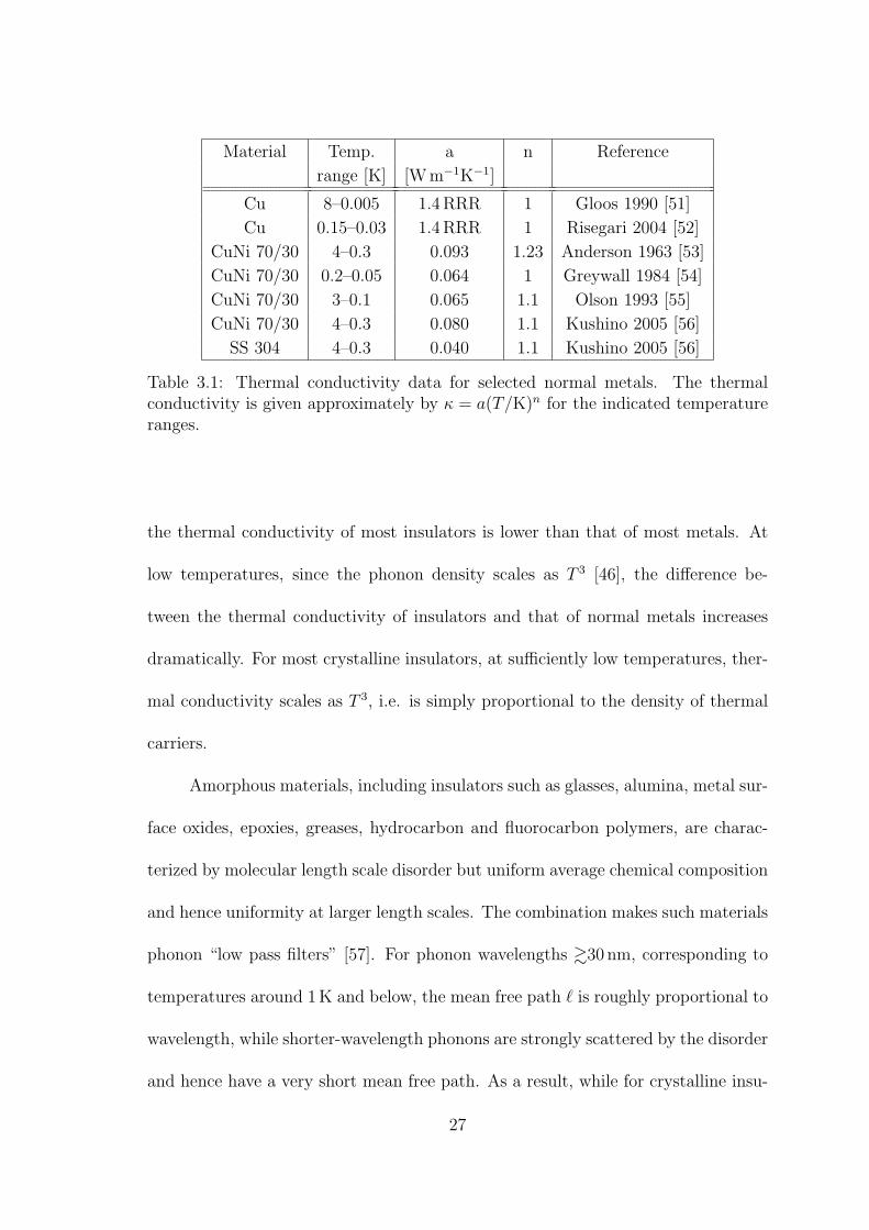
Material Temp. a n Reference
range [K] [W m−1K−1]
Cu 8–0.005 1.4 RRR 1 Gloos 1990 [51]
Cu 0.15–0.03 1.4 RRR 1 Risegari 2004 [52]
CuNi 70/30 4–0.3 0.093 1.23 Anderson 1963 [53]
CuNi 70/30 0.2–0.05 0.064 1 Greywall 1984 [54]
CuNi 70/30 3–0.1 0.065 1.1 Olson 1993 [55]
CuNi 70/30 4–0.3 0.080 1.1 Kushino 2005 [56]
SS 304 4–0.3 0.040 1.1 Kushino 2005 [56]
Table 3.1: Thermal conductivity data for selected normal metals. The thermalconductivity is given approximately by κ = a(T/K)n for the indicated temperatureranges.
the thermal conductivity of most insulators is lower than that of most metals. At
low temperatures, since the phonon density scales as T 3 [46], the difference be-
tween the thermal conductivity of insulators and that of normal metals increases
dramatically. For most crystalline insulators, at sufficiently low temperatures, ther-
mal conductivity scales as T 3, i.e. is simply proportional to the density of thermal
carriers.
Amorphous materials, including insulators such as glasses, alumina, metal sur-
face oxides, epoxies, greases, hydrocarbon and fluorocarbon polymers, are charac-
terized by molecular length scale disorder but uniform average chemical composition
and hence uniformity at larger length scales. The combination makes such materials
phonon “low pass filters” [57]. For phonon wavelengths &30 nm, corresponding to
temperatures around 1 K and below, the mean free path ℓ is roughly proportional to
wavelength, while shorter-wavelength phonons are strongly scattered by the disorder
and hence have a very short mean free path. As a result, while for crystalline insu-
27
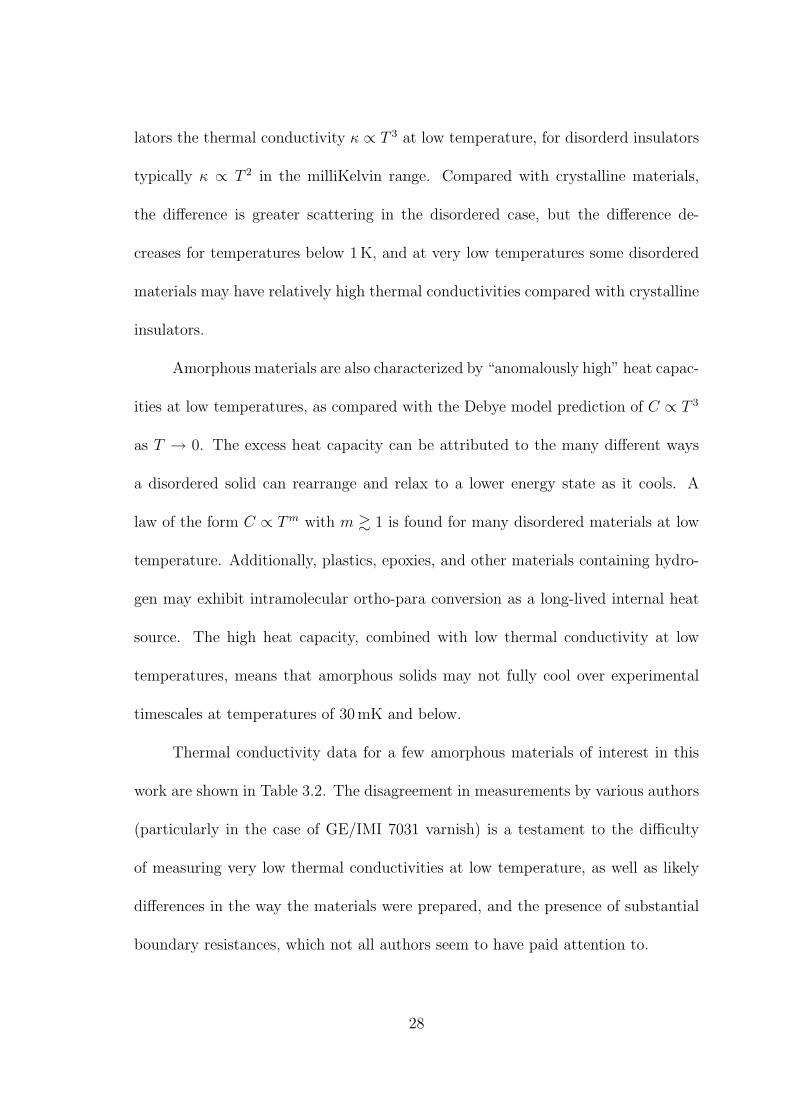
lators the thermal conductivity κ ∝ T 3 at low temperature, for disorderd insulators
typically κ ∝ T 2 in the milliKelvin range. Compared with crystalline materials,
the difference is greater scattering in the disordered case, but the difference de-
creases for temperatures below 1 K, and at very low temperatures some disordered
materials may have relatively high thermal conductivities compared with crystalline
insulators.
Amorphous materials are also characterized by “anomalously high” heat capac-
ities at low temperatures, as compared with the Debye model prediction of C ∝ T 3
as T → 0. The excess heat capacity can be attributed to the many different ways
a disordered solid can rearrange and relax to a lower energy state as it cools. A
law of the form C ∝ Tm with m & 1 is found for many disordered materials at low
temperature. Additionally, plastics, epoxies, and other materials containing hydro-
gen may exhibit intramolecular ortho-para conversion as a long-lived internal heat
source. The high heat capacity, combined with low thermal conductivity at low
temperatures, means that amorphous solids may not fully cool over experimental
timescales at temperatures of 30 mK and below.
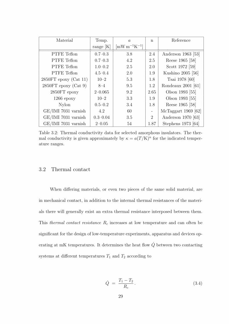
Thermal conductivity data for a few amorphous materials of interest in this
work are shown in Table 3.2. The disagreement in measurements by various authors
(particularly in the case of GE/IMI 7031 varnish) is a testament to the difficulty
of measuring very low thermal conductivities at low temperature, as well as likely
differences in the way the materials were prepared, and the presence of substantial
boundary resistances, which not all authors seem to have paid attention to.
28
Material Temp. a n Reference
range [K] [mW m−1K−1]
PTFE Teflon 0.7–0.3 3.8 2.4 Anderson 1963 [53]
PTFE Teflon 0.7–0.3 4.2 2.5 Reese 1965 [58]
PTFE Teflon 1.0–0.2 2.5 2.0 Scott 1972 [59]
PTFE Teflon 4.5–0.4 2.0 1.9 Kushino 2005 [56]
2850FT epoxy (Cat 11) 10–2 5.3 1.8 Tsai 1978 [60]
2850FT epoxy (Cat 9) 8–4 9.5 1.2 Rondeaux 2001 [61]
2850FT epoxy 2–0.065 9.2 2.65 Olson 1993 [55]
1266 epoxy 10–2 3.3 1.9 Olson 1993 [55]
Nylon 0.5–0.2 3.4 1.8 Reese 1965 [58]
GE/IMI 7031 varnish 4.2 60 - McTaggart 1969 [62]
GE/IMI 7031 varnish 0.3–0.04 3.5 2 Anderson 1970 [63]
GE/IMI 7031 varnish 2–0.05 54 1.87 Stephens 1973 [64]
Table 3.2: Thermal conductivity data for selected amorphous insulators. The ther-mal conductivity is given approximately by κ = a(T/K)n for the indicated temper-ature ranges.
3.2 Thermal contact
When differing materials, or even two pieces of the same solid material, are
in mechanical contact, in addition to the internal thermal resistances of the materi-
als there will generally exist an extra thermal resistance interposed between them.
This thermal contact resistance Rc increases at low temperature and can often be
significant for the design of low-temperature experiments, apparatus and devices op-
erating at mK temperatures. It determines the heat flow Q between two contacting
systems at different temperatures T1 and T2 according to
Q =T1 − T2
Rc
. (3.4)
29
If the contact is uniform over the area A, the area-independent contact resistiv-
ity1 may be defined as Rc ≡ RcA. Eq. 3.4 can also be written in terms of the heat
per unit area q ≡ Q/A.
Note that this definition of Rc implies that it could be a function of both
temperatures, and on theoretical grounds (see below) we should expect that this
will be the case. However, we usually linearize and write
q = ∆T / Rc(T ) , (3.5)
where ∆T ≡ T1 − T2, and T can be defined as the average of T1 and T2, on the
assumption that ∆T ≪ T .
The contact resistivity Rc can considered a macroscopic quantity, and, as a
matter of convenience, can be defined equally well for contacts of any type, includ-
ing “sandwiches” filled with (defined amounts of) glue, solder, grease, dirt or other
materials. In these cases, Rc will generally include a component from the volume
thermal resistance of the filling material. I will distinguish between Rc and the in-
trinsic thermal boundary (Kapitza) resistivity RK of an interface between dissimilar
materials. The latter is a microscopic quantity which gives rise to a discontinuous
temperature profile across a perfectly clean and gap-free boundary. It is completely
distinct from the volume thermal resistance of either material.
The Kapitza resistance RK is of theoretical interest but is less closely related
1In much of the literature, the symbol RK (or RB) is defined as an area-independent property ofa given type of interface, but this leads to confusion in its use. I hew to the more general conventionthat a resistance is the inverse of a conductance, and incorporates all geometrical factors. Hence,where the distinction matters, I will write the area-independent contact resitivity as Rc, and myRc is a resistance, Rc = Rc/A. I use the same convention for the Kapitza component of Rc,RK = RK/A
30
to Rc than one would like. Although a complicated and often obscure subject,
which is susceptible to possibly endless refinement, simple models for RK do yield
qualititatively and, less often, quantitatively accurate results in some, well-controlled
cases. However, using these models to predict Rc in situations of practical interest
is often impractical or impossible, because of variables such as surface condition,
contaminants, and the area of actual contact between rough surfaces. Thus, in
practice, empirical data is the best guide to estimating Rc, and even this is often
unreliable (or unavailable).
Historically, the temperature discontinuity that arises across the boundary
between two media when heat flows across was first observed at interfaces between
metals and liquid helium (LHe) in the superfluid state [65], and measurements for
superfluid LHe-bronze were reported by Kapitza in 1941 [5]. The term “Kapitza
resistance” may refer specifically to the large RK between solids and (normal or
superfluid) LHe, but is also often applied to RK between different solids.
The Kapitza resistance is a particular problem in the design of helium liquefiers
and LHe-based refrigerators. The solution there is to provide a large contacting
surface between metal parts and LHe that is to cool, or be cooled by, the metal,
usually using porous sintered Cu or Ag powder. This is generally not needed at
4 K, but becomes necessary below 1 K. Thus, for example, a block of sintered Cu
immersed in the 4He/3He mix at the bottom of the mixing chamber provides the
thermal link to the cold plate in our dilution fridge, and sintered Ag is used in some
of the heat exchangers.
31
3.2.1 Kapitza resistance: Theory
Khalatnikov in 1952 provided an explanation for the Kapitza resistance in
terms of an acoustic mismatch between the different media [66]. This acoustic mis-
match model (AMM) was developed independently by Mazo and Onsager [67], and
extended to solid-solid interfaces by Little [68]. It predicts a T−3 dependence for
RK when only phonons are involved, which is generally observed experimentally, but
with strong deviations. Poor quantitative agreement between the AMM and exper-
imental data, particularly for Kapitza (solid-LHe) boundaries, led many researchers
to attempt improvement of the AMM by considering the role of phonon absorbtion
by electrons, and scattering by various mechanisms at or near the boundary (which
in most cases will reduce RK by providing a parallel channel for transport across
the boundary) [69, 70, 5]. The mixed and inconsistent results, obtained from fairly
detailed calculations, led Swartz in 1989 [70] to propose a simple alternative, the
diffuse mismatch model (DMM). According to the DMM, all phonons are strongly
scattered at the boundary, making acoustic mismatch irrelevant.
Despite its independent reasoning, the DMM agrees remarkably well with the
AMM for metal-dielectric interfaces. For clean and well-characterized interfaces, the
measured RK usually lies between the values predicted by the AMM and DMM. The
two models can can be considered as two limiting cases [70]. Alternatively, phonon
transmission with and without scattering can be considered parallel channels. For
Kapitza boundaries, in the absence of scattering, acoustic mismatch severely re-
stricts transmission. The presence of scattering therefore opens up a larger channel.
32
In this case, the DMM predicts an RK close to experimentally observed values, while
the AMM prediction is up to two orders of magnitude too high.
Boundary resistance measurements are in general difficult and poorly repro-
ducible, and unfortunately no simple model provides an adequate basis for quantita-
tive prediction in the cases of greatest interest here: metal-metal and metal-dielectric
interfaces with unknown effects of surface roughness, disorder and damage, and ox-
ides and other contaminants.
For the benefit of understanding, adapting the treatments of Little [68], Pe-
terson [69], and Swartz [70], I sketch the acoustic mismatch and diffuse mismatch
models in their simplest forms, taking account of longitudinal phonons only. The
extension to take account of transverse modes in solids is straightforward, but com-
plicates the notation and would tend to obscure the theory.
Consider the boundary between media M1 and M2 at temperatures T1 and T2.
Phonons from each medium collide with the boundary and are either reflected back
or transmitted into the other medium, creating thermal currents q1 from M1 to M2
and q2 from M2 to M1, per unit area of the boundary. The net heat transfer is then
q = q1 − q2 . (3.6)
Thermodynamics requires that q = 0 when T1 = T2.
According to Snell’s law2, for phonons from M1 which are incident on the
boundary at an angle θ1 relative to normal, and which propagate into M2 at θ2, we
have v1 sin θ2 = v2 sin θ1, where vj is the phonon (group) velocity in Mj. Further-
2Actually, the law of refraction was described correctly by ibn Sahl of Baghdad circa 984 [71].
33
more, the fraction α1 of such phonons which are transmitted is derived in classical
wave theory (acoustic Fresnel equations) by matching pressures and normal compo-
nents of velocity on each side of the boundary [72]. The result [68] is
α1(θ1) = 4ρ2v2
ρ1v1
· cos θ2
cos θ1
·(
ρ2v2
ρ1v1
+cos θ2
cos θ1
)−2
, (3.7)
where ρj is the mass density of Mj. Note that this form is invariant on exchange of
indices, since a−1b−1(a−1 + b−1)−2 = ab (a+ b)−2. Thus α1(θ1) = α2(θ2), as required
by the principle of microscopic reversibility.
If the density of longitudinal phonons in M1 is N1(ω, T1), where ω is the phonon
angular frequency, then the total rate at which these phonons are delivered to a unit
area of the boundary will be
∫ ∞
0
dω
∫ π/2
0
2π sin θ1 dθ1
1
4πv1 cos θ1 N1(ω, T1)
, (3.8)
where the factor1
4πnormalizes for the sphere of phonon propagation directions,
v1 cos θ1 is the normal component of the phonon velocity, and 2π sin θ1 dθ1 is the
differential solid angle. Inserting the transmission probability α1(θ1) and the phonon
energy ~ω gives the expression for q1, which can be written as:
q1 =
∫ ∞
0
~ω N1(ω) dω · v1
2·∫ π/2
0
α1(θ1) cos θ1 sin θ1 dθ1 . (3.9)
Using the Debye approximation (for a single mode)
N1(ω, T1) =ω2
2π2v31
· 1
e~ω/kBT1 − 1, (3.10)
34
in the low-temperature limit [46], the first integral becomes
∫ ∞
0
~ω
2π2v31
· ω2 dω
e~ω/kBT − 1=
~
2π2v31
·(kBT1
~
)4∫ ∞
0
z3 dz
ez − 1
=k4
B T 41
2π2~3v31
· π4
15. (3.11)
The second integral in Eq. 3.9
Γ1
(v1
v2
,ρ1
ρ2
)
≡∫ π/2
0
α1(θ1) cos θ1 sin θ1 dθ1 (3.12)
is a complicated function of the indicated ratios, and is the transmission rate in the
sense thatv1
2· Γ1 is the effective velocity of flow of the phonon gas of M1 across
the boundary into M2. The maximum value of Γ1 = 1
2is always obtained with
v1 = v2 and ρ1 = ρ2, but matching of the acoustic impedance, v1ρ1 = v2ρ2, does
not maximize Γ1, nor q ∝ Γ1/v21, when v2 > v1. Thus, the acoustic mismatch is not
precisely an “impedance mismatch.”
As previously noted, if T1 = T2 we must have q1 = q2. Given that q1 is a
function of T1 but not of T2, and vice versa, this implies that q2(T ) = q1(T ) for any
temperature T . Thus, from Eqs. 3.6 and 3.9–3.12,
q =π2k4
B
60~3· Γ1
v21
· (T 41 − T 4
2 ) . (3.13)
It may seem puzzling that this result appears to be asymmetrical with regard
to M1 and M2, but Γ1 contains information about both media. With Γ2 defined as
in Eq. 3.12 with the exchange of all indices, the symmetry is that Γ2/v22 = Γ1/v
21.
To put the result into the form of Eq. 3.5, we assume that ∆T ≪ T1, T2. This
is a risky assumption at low temperatures, but can only lead to an underestimate
35
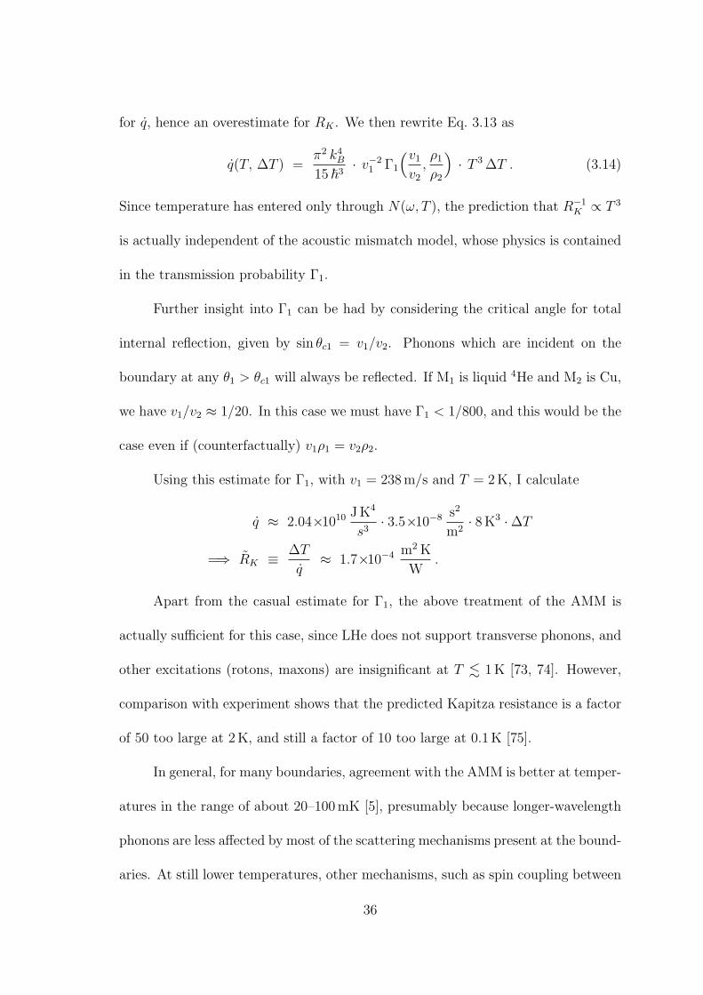
for q, hence an overestimate for RK . We then rewrite Eq. 3.13 as
q(T, ∆T ) =π2 k4
B
15 ~3· v−2
1 Γ1
(v1
v2
,ρ1
ρ2
)
· T 3 ∆T . (3.14)
Since temperature has entered only through N(ω, T ), the prediction that R−1
K ∝ T 3
is actually independent of the acoustic mismatch model, whose physics is contained
in the transmission probability Γ1.
Further insight into Γ1 can be had by considering the critical angle for total
internal reflection, given by sin θc1 = v1/v2. Phonons which are incident on the
boundary at any θ1 > θc1 will always be reflected. If M1 is liquid 4He and M2 is Cu,
we have v1/v2 ≈ 1/20. In this case we must have Γ1 < 1/800, and this would be the
case even if (counterfactually) v1ρ1 = v2ρ2.
Using this estimate for Γ1, with v1 = 238 m/s and T = 2 K, I calculate
q ≈ 2.04×10¹⁰ J K4
s3· 3.5×10−8 s2
m2· 8 K3 · ∆T
=⇒ RK ≡ ∆T
q≈ 1.7×10⁻⁴ m2 K
W.
Apart from the casual estimate for Γ1, the above treatment of the AMM is
actually sufficient for this case, since LHe does not support transverse phonons, and
other excitations (rotons, maxons) are insignificant at T . 1 K [73, 74]. However,
comparison with experiment shows that the predicted Kapitza resistance is a factor
of 50 too large at 2 K, and still a factor of 10 too large at 0.1 K [75].
In general, for many boundaries, agreement with the AMM is better at temper-
atures in the range of about 20–100 mK [5], presumably because longer-wavelength
phonons are less affected by most of the scattering mechanisms present at the bound-
aries. At still lower temperatures, other mechanisms, such as spin coupling between
36
3He and metals or paramagnetic salts, and the formation of solid He surface layers,
may intervene to reduce RK [66, 49].
The AMM can be considered a limiting case in which no phonon scattering
occurs at the boundary. Because scattering does in general play an important role,
Swartz proposed, as an alternative limiting case, the diffuse mismatch model, in
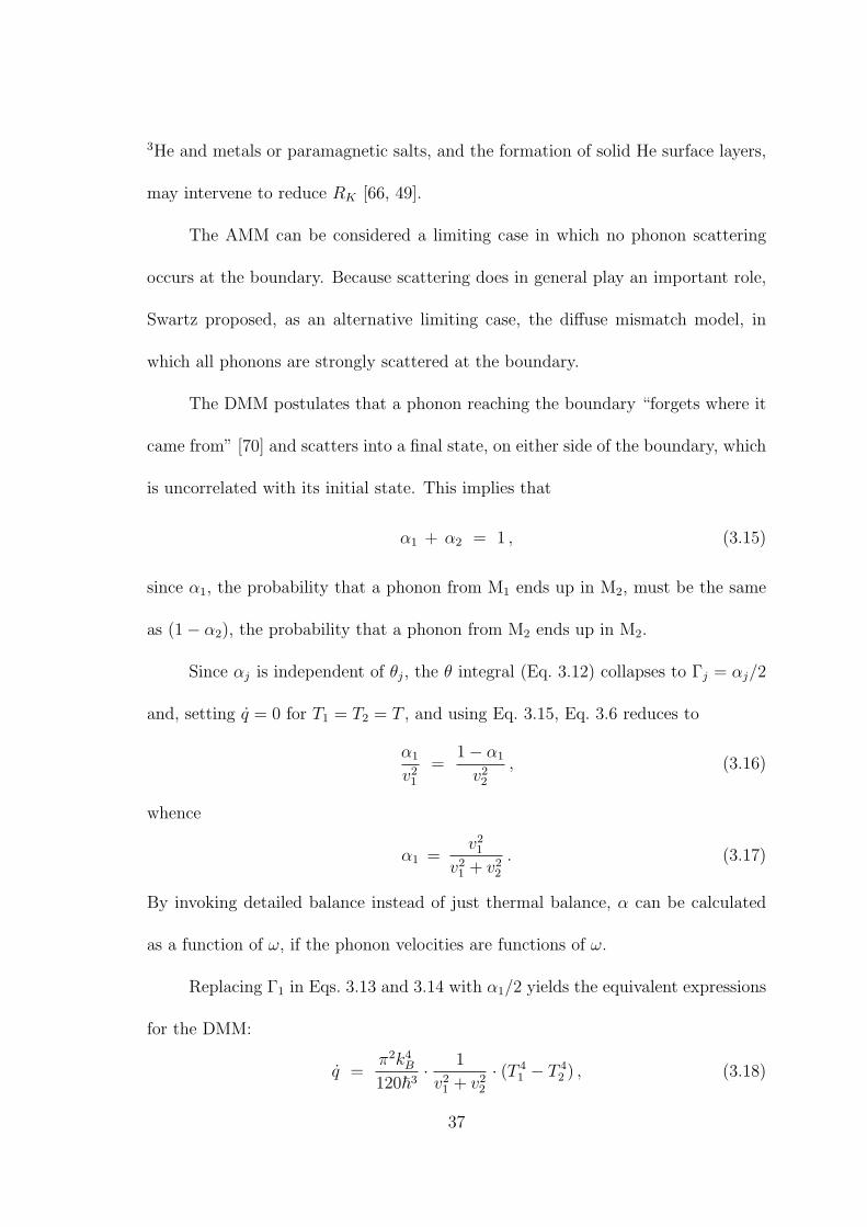
which all phonons are strongly scattered at the boundary.
The DMM postulates that a phonon reaching the boundary “forgets where it
came from” [70] and scatters into a final state, on either side of the boundary, which
is uncorrelated with its initial state. This implies that
α1 + α2 = 1 , (3.15)
since α1, the probability that a phonon from M1 ends up in M2, must be the same
as (1 − α2), the probability that a phonon from M2 ends up in M2.
Since αj is independent of θj, the θ integral (Eq. 3.12) collapses to Γj = αj/2
and, setting q = 0 for T1 = T2 = T , and using Eq. 3.15, Eq. 3.6 reduces to
α1
v21
=1 − α1
v22
, (3.16)
whence
α1 =v2
1
v21 + v2
2
. (3.17)
By invoking detailed balance instead of just thermal balance, α can be calculated
as a function of ω, if the phonon velocities are functions of ω.
Replacing Γ1 in Eqs. 3.13 and 3.14 with α1/2 yields the equivalent expressions
for the DMM:
q =π2k4
B
120~3· 1
v21 + v2
2
· (T 41 − T 4
2 ) , (3.18)
37
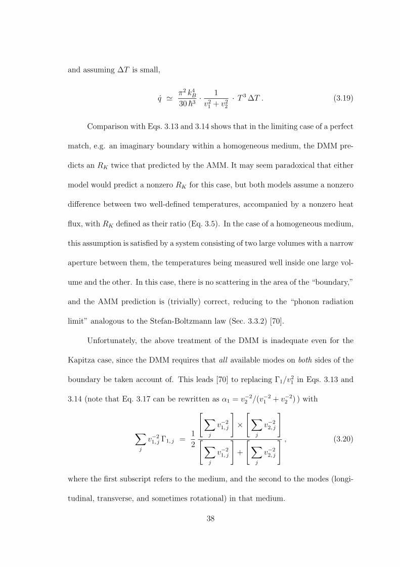
and assuming ∆T is small,
q ≃ π2 k4B
30 ~3· 1
v21 + v2
2
· T 3 ∆T . (3.19)
Comparison with Eqs. 3.13 and 3.14 shows that in the limiting case of a perfect
match, e.g. an imaginary boundary within a homogeneous medium, the DMM pre-
dicts an RK twice that predicted by the AMM. It may seem paradoxical that either
model would predict a nonzero RK for this case, but both models assume a nonzero
difference between two well-defined temperatures, accompanied by a nonzero heat
flux, with RK defined as their ratio (Eq. 3.5). In the case of a homogeneous medium,
this assumption is satisfied by a system consisting of two large volumes with a narrow
aperture between them, the temperatures being measured well inside one large vol-
ume and the other. In this case, there is no scattering in the area of the “boundary,”
and the AMM prediction is (trivially) correct, reducing to the “phonon radiation
limit” analogous to the Stefan-Boltzmann law (Sec. 3.3.2) [70].
Unfortunately, the above treatment of the DMM is inadequate even for the
Kapitza case, since the DMM requires that all available modes on both sides of the
boundary be taken account of. This leads [70] to replacing Γ1/v21 in Eqs. 3.13 and
3.14 (note that Eq. 3.17 can be rewritten as α1 = v−22 /(v−2
1 + v−22 ) ) with
∑
j
v−21, j Γ1, j =
1
2
[
∑
j
v−21, j
]
×[
∑
j
v−22, j
]
[
∑
j
v−21, j
]
+
[
∑
j
v−22, j
] , (3.20)
where the first subscript refers to the medium, and the second to the modes (longi-
tudinal, transverse, and sometimes rotational) in that medium.
38
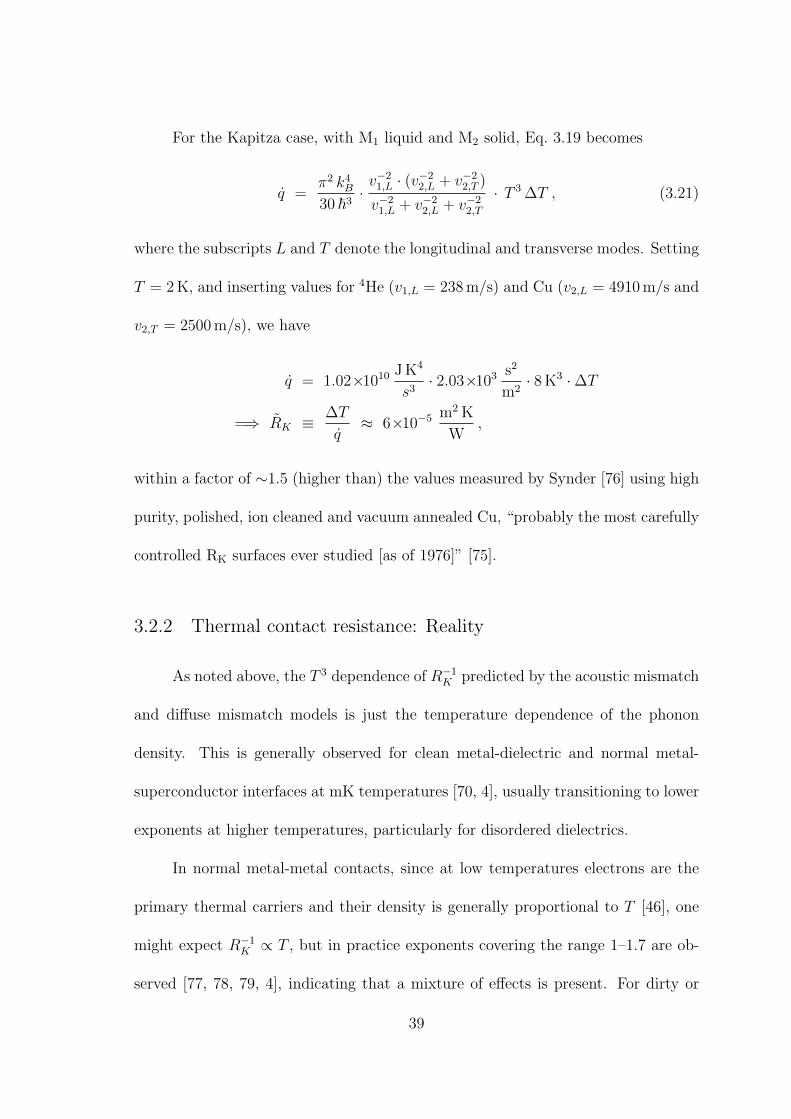
For the Kapitza case, with M1 liquid and M2 solid, Eq. 3.19 becomes
q =π2 k4
B
30 ~3·v−2
1,L · (v−2
2,L + v−2
2,T )
v−2
1,L + v−2
2,L + v−2
2,T
· T 3 ∆T , (3.21)
where the subscripts L and T denote the longitudinal and transverse modes. Setting
T = 2 K, and inserting values for 4He (v1,L = 238 m/s) and Cu (v2,L = 4910 m/s and
v2,T = 2500 m/s), we have
q = 1.02×10¹⁰ J K4
s3· 2.03×103 s2
m2· 8 K3 · ∆T
=⇒ RK ≡ ∆T
q≈ 6×10⁻⁵ m2 K
W,
within a factor of ∼1.5 (higher than) the values measured by Synder [76] using high
purity, polished, ion cleaned and vacuum annealed Cu, “probably the most carefully
controlled RK surfaces ever studied [as of 1976]” [75].
3.2.2 Thermal contact resistance: Reality
As noted above, the T 3 dependence of R−1
K predicted by the acoustic mismatch
and diffuse mismatch models is just the temperature dependence of the phonon
density. This is generally observed for clean metal-dielectric and normal metal-
superconductor interfaces at mK temperatures [70, 4], usually transitioning to lower
exponents at higher temperatures, particularly for disordered dielectrics.
In normal metal-metal contacts, since at low temperatures electrons are the
primary thermal carriers and their density is generally proportional to T [46], one
might expect R−1
K ∝ T , but in practice exponents covering the range 1–1.7 are ob-
served [77, 78, 79, 4], indicating that a mixture of effects is present. For dirty or
39
deliberately greased metal-metal contacts, thermal conductivity across the bound-
ary may be limited by the presence of disordered, electrically insulating or semi-
conducting material, for which the expected temperature exponent at temperatures
near 1 K would be about 2. For sufficiently thick layers of insulating material sand-
wiched between metals, e.g. very dirty, glued or heavily greased joints, RK for the
two metal-insulator boundaries may be dominated by the volume thermal resistance
of the insulator.
The magnitude of R−1c in metal-metal contacts is not reliably predicted by
the Wiedemann-Franz-Lorenz law (Eq. 3.3), but can be up to 105 times greater
[4], consistent with the presence of electrically insulating oxides and other contami-
nants, and the possible role of electrons not only as direct thermal carriers but also
as mediators of phonon scattering and absorbtion. However, Didschuns et al. [79]
measured thermal conductivity for bolted contacts between Au surfaces plated on
Cu in the temperature range 90–400 mK, and observed roughly linear temperature
dependence. Although they did not measure the electrical resistances of their junc-
tions, they argued that the results were of the correct magnitude to be consistent
with the WFL law, as might be expected for clean metal-metal junctions.
Whenever preformed solid surfaces (metal-metal or metal-dielectric) are pressed
together, due to surface roughness the area of actual contact is initially (at low pres-
sure) a small fraction of the gross surface area. The fraction is often quoted as of
order 10−6 for metal-metal contacts [49, 4, 5], but the basis for this number is ob-
scure, and a recent review quotes “1–2 %” [80]. In reality, the fraction is strongly
pressure-dependent.
40
Solid materials can generally be characterized by a pressure Y (hardness, or
yield strength) above which, when the pressure is locally applied to a region of the
surface, the material will yield and break or deform. This can be thought of as
analogous to a taut balloon whose internal pressure (repulsive force) is balanced
against the tension of its skin (cohesive force). When external pressure applied
locally to the skin of the balloon exceeds the internal pressure, the balloon yields.
For rough surfaces in contact, this means that under an applied force F the
asperities of one surface will blunt or dig into the other, depending on relative
hardnesses and microscopic details. As as result, regardless of the gross area A of
the surfaces, the area S of actual contact is expected to increase until
F = Y S . (3.22)
Hence, assuming that Rc ∝ S−1, we may expect Rc ∝ F−1, and thus be independent
of the gross area of the contacting surfaces.
Berman and Mate [77] found that Q for Cu-Cu contacts varied as F 0.88 at
4.2 K and as F 0.58 at 18 K, with F ranging from about 10 to 103 N. They suggested
that the deviation from Q ∝ F might be attributable to differences between plastic
deformation upon compression and elastic relaxation upon decompression, but this
hypothesis was inconsistent with the lack of appreciable differences between the data
taken with force increasing and decreasing. In contrast, Colwell [78] observed Q/F
constant for (superconducting) In-Cu contacts, with F ranging from 20–80 N and T
ranging from 0.3–2 K.
However, because the “balloon” analogy ignores the effects of crystalline or
41
other microscopic structure, and possible dependences on the scale and shape of
surface roughness, Y must be considered an effective parameter which could at
best be only roughly estimated from tabulated values of hardness or yield strength
(as determined by macroscopic measurements, according to any of several opera-
tional definitions). In addition, the linearity of Eq. 3.22 cannot continue to hold
as F −→ Y A, since the gross area A (times some factor of order unity) will set an
upper bound on S.
For sufficiently soft materials, e.g. In, PTFE and certainly grease pressed
against or between metals or other hard materials, a limit may be approached in
which Rc is nearly independent of F .
However, even in these cases, trapped gases, oxides and other contaminants
will still affect the reproducibility of Rc. In addition, this discussion has ignored the
effects of damage to due to fracture or plastic deformation under pressure, which
may either increase or decrease both the microscopic RK and the macroscopic Rc
[5]. There may also be effects dependent on the microscopic size of the contacting
areas [77].
Given all these complexities, in practice metal-metal and metal-insulator ther-
mal contact resistances are not predictable from theory, even when the materials
are well-bonded, much less when pressed together. Instead, empirical data must
be consulted when it is available, and used with caution given uncertainties about
the condition of surfaces. Gmelin et al. [80] provide the most complete review of
solid-solid contact resistances I have found, covering general principles and data for
a wide range of materials.
42
If a reference value is known, extrapolation is possible within a limited range,
based on observed or predicted dependences on temperature and pressure. However,
one should remember that, for example, a phenomenon that is governed by a sum
of quadratic and cubic terms may fit, over a limited range, to a power law with an
exponent between two and three. The fact that a good fit is obtained within some
given range does not imply that the phenomenon does not deviate from the reported
power law immediately outside the reported range; it may imply the opposite.
3.2.3 Estimation of thermal boundary resistance: Empirical data
Anderson and Peterson [63] measured contact resistances Rc at temperatures of
0.3–0.04 K for several materials commonly used as low-temperature thermal bonding
agents, including Apiezon N grease, RTV silicone, Epibond 121 epoxy, and super-
conducting In solder. They sought to separate the boundary resistances from the
volume resistances of the bonding agents by fitting their data to assumed T−3 terms
for the boundary resistances, plus T−n terms for the volume resistances, with n = 2
usually assumed for amorphous materials. Their “most striking result” was that
RK ≃ 0.75 (T/K)−3 m2 K W−1 “for all materials within ±20%.”
In contrast, Colin [81] measured Rc for In solder and epoxy bonds with and
without silver fill. The In bonds exhibited R−1c ∝ T 3 over T = 4 − 0.3 K whereas
the epoxy bonds exhibited close to R−1c ∝ T 2 over the same range. Below 1 K, the
epoxy bonds had lower resistance than the indium bonds, and silver-filled epoxy
lower resistance than unfilled. It is not clear whether this is due to the “contact
43
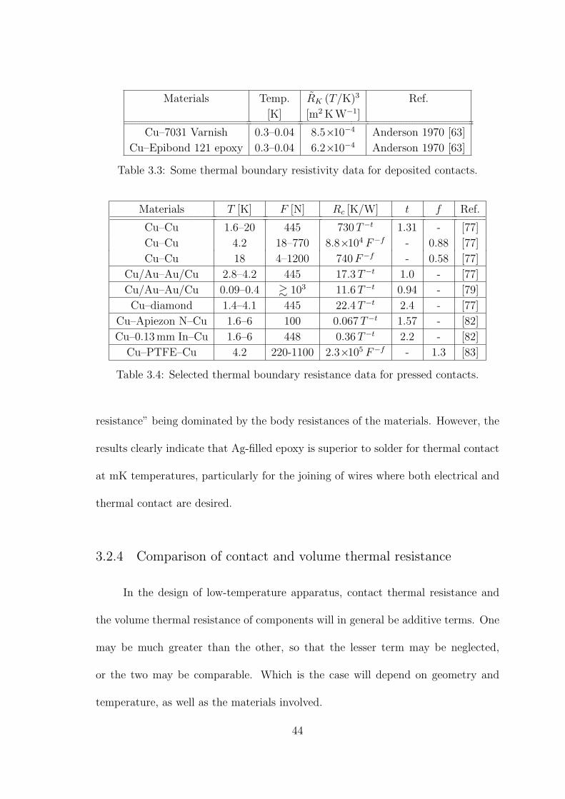
Materials Temp. RK (T/K)3 Ref.
[K] [m2 K W−1]
Cu–7031 Varnish 0.3–0.04 8.5×10⁻⁴ Anderson 1970 [63]
Cu–Epibond 121 epoxy 0.3–0.04 6.2×10⁻⁴ Anderson 1970 [63]
Table 3.3: Some thermal boundary resistivity data for deposited contacts.
Materials T [K] F [N] Rc [K/W] t f Ref.
Cu–Cu 1.6–20 445 730T−t 1.31 - [77]
Cu–Cu 4.2 18–770 8.8×10⁴ F−f - 0.88 [77]
Cu–Cu 18 4–1200 740F−f - 0.58 [77]
Cu/Au–Au/Cu 2.8–4.2 445 17.3T−t 1.0 - [77]
Cu/Au–Au/Cu 0.09–0.4 & 103 11.6T−t 0.94 - [79]
Cu–diamond 1.4–4.1 445 22.4T−t 2.4 - [77]
Cu–Apiezon N–Cu 1.6–6 100 0.067T−t 1.57 - [82]
Cu–0.13 mm In–Cu 1.6–6 448 0.36T−t 2.2 - [82]
Cu–PTFE–Cu 4.2 220-1100 2.3×10⁵ F−f - 1.3 [83]
Table 3.4: Selected thermal boundary resistance data for pressed contacts.
resistance” being dominated by the body resistances of the materials. However, the
results clearly indicate that Ag-filled epoxy is superior to solder for thermal contact
at mK temperatures, particularly for the joining of wires where both electrical and
thermal contact are desired.
3.2.4 Comparison of contact and volume thermal resistance
In the design of low-temperature apparatus, contact thermal resistance and
the volume thermal resistance of components will in general be additive terms. One
may be much greater than the other, so that the lesser term may be neglected,
or the two may be comparable. Which is the case will depend on geometry and
temperature, as well as the materials involved.
44
Consider the case of a cube with sides of length ℓ made of some material with
volume thermal conductivity κ. Its volume thermal resistance RV will be given by
RV = κ−1ℓ−1. If it contacts another object on one face, through a contact resistivity
Rc, the contact resistance will be Rc = Rc ℓ−2. Thus, Rc/RV = ℓ−1 κ Rc, and we
see that the relative importance of contact resistance will decrease for larger objects
with proportionately larger contact areas.
A useful measure of comparison is the thickness ℓ∗(T ) ≡ κRc of a layer of ma-
terial, contacting another material, whose volume thermal resistance perpendicular
to the plane of contact is equal to the contact thermal resistance.
Pressed Cu-Cu: A case of interest here is Cu components bolted to the Au-plated
Cu cold plates of our dilution fridge. I will consider first Cu-Cu junctions in the
same geometry. Oxford provides M3 bolt holes in a 15 mm square lattice, i.e. one
bolt hole per 2.25×10⁻⁴ m2 of area. The maximum load that stainless steel M3 bolts
will support is about 1.6 kN [4], which should be derated to about 1 kN to avoid the
risk of breaking.
Berman and Mate [77] measured Rc for Cu-Cu contacts under forces in the
range of 101–103 N and over temperatures in the range of 1.6–20 K. Presumably their
samples were as clean as could reasonably be achieved, but they did not report any
special cleaning measures, and did report that they believed oxides were present
(as they necessarily would be, given that the samples were prepared in air). For
F =445 N (100 lbf), they obtained Rc = 730 (T/K)−1.3 K/W. Whether this can be
extrapolated an order of magnitude lower in temperature is questionable, but the
45
power law fit was good over the more than one order of magnitude range of their
measurements.
While the total force F applied to the junction, rather than the pressure,
determines Rc, to compute ℓ∗ we need Rc, and thus we must specify the area over
which the force is applied. To match Berman and Mate’s F =445 N, the area of the
junction can be set at 1×10⁻⁴ m2, yielding Rc = 0.073 (T/K)−1.3 m2K/W.
From these data, using κ = L0 T/ρ = 140 (T/K) W m−1K−1 for OFHC Cu
with RRR=100 (Table 3.1) we calculate ℓ∗ = κ Rc ≃ 10 (T/K)−0.3 m. This means
that, under the stated assumptions, contact thermal resistance dominates volume
thermal resistance when OFHC Cu is broken by a pressed Cu-Cu contact at LHe or
mK temperatures. An example would be a (15 mm)2 square Cu bar bolted at one
end to a Cu cold plate with a single M3 bolt; only if the bar were 10 m long would
the volume resistance compare with the contact resistance at T . 1 K.
Au plated Cu: As mentioned above, the cold plates of our dilution fridge are
Au-plated Cu. Some parts that are bolted to the cold plates are Cu only, and others
are Au-plated Cu. Berman and Mate [77] found Rc = 17(T/K)−1 K/W for Cu/Au–
Au/Cu contacts under 445 N force at T = 2.8− 4.2 K, which agrees reasonably well
with Didschuns et al. [79], who found Rc = 12(T/K)−0.94 K/W over T = 90−400 mK
under somewhat greater force. Note that any boundary resistance between the Au
plating and the bulk Cu has been taken into account by the data and is expected
to be small, since electrons will be the dominant thermal carriers.
Using Berman and Mate’s result, we predict for Cu/Au–Au/Cu at low tem-
46
peratures ℓ∗ ≃ 20 cm. Thus, the effect of Au plating is to lower Rc by a factor of up
to ∼40 at 1 K, ∼80 at 0.1 K, and ∼120 at 30 mK. In the latter case, we will have ℓ∗
the order of 1 mm, so the volume resistivity of OFHC Cu will generally dominate the
contact resistance for Au-plated Cu at the base temperature of our dilution fridge.
When only one of the Cu surfaces is plated, we may expect that Rc for the
Cu/Au–Cu contact will be roughly half of Rc for a Cu–Cu contact under the same
force, assuming that the contact resistance is mostly due to the presence of oxides,
contaminants and gaps between the asperities of the (usually harder) Cu. Thus in
most cases it will make little sense to plate only one surface.
Cu-Apiezon N-Cu: Where higher Rc can be tolerated or Au plating is unavailable,
Cu–Cu contacts are often greased. Apiezon NTM is a popular type of thin-spreading,
low-viscosity grease used especially for thermal contact. The ideal amount of grease
would be just enough to fill the voids between contacting asperities, thus providing
additional thermal contact without reducing metal-metal contact. In practice it
is impossible to control the amount of grease so precisely, but if excess grease is
expelled from the junction under pressure, its viscosity will roughly determine a
limiting thickness. One then obtains a Cu–grease–Cu sandwich, with an Rc that is
not strongly dependent on the applied force [82].
Anderson and Peterson [63] measured Rc for a Cu-Apiezon N-Cu sandwich
with grease thickness ℓ = 6.4 µm, over the temperature range 40–500 mK. They fit
this data to the form Rc = aT−3 + bℓT−2, under the assumption that these terms
would represent the boundary and volume resistances respectively, finding that
47
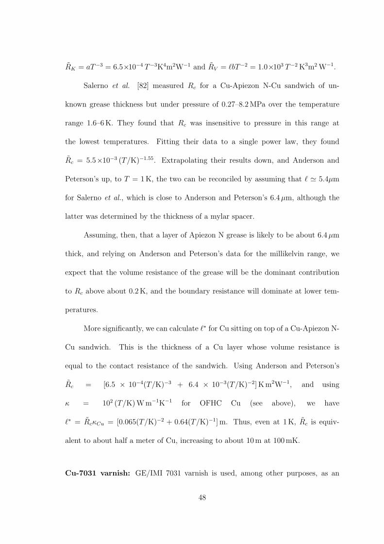
RK = aT−3 = 6.5×10⁻⁴ T−3K4m2W−1 and RV = ℓbT−2 = 1.0×10³ T−2 K3m2 W−1.
Salerno et al. [82] measured Rc for a Cu-Apiezon N-Cu sandwich of un-
known grease thickness but under pressure of 0.27–8.2 MPa over the temperature
range 1.6–6 K. They found that Rc was insensitive to pressure in this range at
the lowest temperatures. Fitting their data to a single power law, they found
Rc = 5.5×10⁻³ (T/K)−1.55. Extrapolating their results down, and Anderson and
Peterson’s up, to T = 1 K, the two can be reconciled by assuming that ℓ ≃ 5.4µm
for Salerno et al., which is close to Anderson and Peterson’s 6.4µm, although the
latter was determined by the thickness of a mylar spacer.
Assuming, then, that a layer of Apiezon N grease is likely to be about 6.4µm
thick, and relying on Anderson and Peterson’s data for the millikelvin range, we
expect that the volume resistance of the grease will be the dominant contribution
to Rc above about 0.2 K, and the boundary resistance will dominate at lower tem-
peratures.
More significantly, we can calculate ℓ∗ for Cu sitting on top of a Cu-Apiezon N-
Cu sandwich. This is the thickness of a Cu layer whose volume resistance is
equal to the contact resistance of the sandwich. Using Anderson and Peterson’s
Rc = [6.5 × 10⁻⁴(T/K)−3 + 6.4 × 10⁻³(T/K)−2] K m2W−1, and using
κ = 102 (T/K) W m−1K−1 for OFHC Cu (see above), we have
ℓ∗ = RcκCu = [0.065(T/K)−2 + 0.64(T/K)−1] m. Thus, even at 1 K, Rc is equiv-
alent to about half a meter of Cu, increasing to about 10 m at 100mK.
Cu-7031 varnish: GE/IMI 7031 varnish is used, among other purposes, as an
48
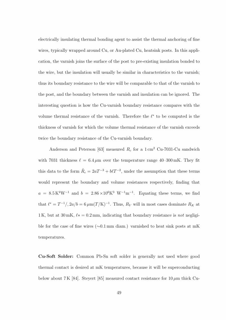
electrically insulating thermal bonding agent to assist the thermal anchoring of fine
wires, typically wrapped around Cu, or Au-plated Cu, heatsink posts. In this appli-
cation, the varnish joins the surface of the post to pre-existing insulation bonded to
the wire, but the insulation will usually be similar in characteristics to the varnish;
thus its boundary resistance to the wire will be comparable to that of the varnish to
the post, and the boundary between the varnish and insulation can be ignored. The
interesting question is how the Cu-varnish boundary resistance compares with the
volume thermal resistance of the varnish. Therefore the ℓ∗ to be computed is the
thickness of varnish for which the volume thermal resistance of the varnish exceeds
twice the boundary resistance of the Cu-varnish boundary.
Anderson and Peterson [63] measured Rc for a 1 cm2 Cu-7031-Cu sandwich
with 7031 thickness ℓ = 6.4 µm over the temperature range 40–300 mK. They fit
this data to the form Rc = 2aT−3 + bℓT−2, under the assumption that these terms
would represent the boundary and volume resistances respectively, finding that
a = 8.5 K4W−1 and b = 2.86×10⁶K3 W−1m−1. Equating these terms, we find
that ℓ∗ = T−1/, 2a/b = 6 µm(T/K)−1. Thus, RV will in most cases dominate RK at
1 K, but at 30 mK, ℓ∗ = 0.2 mm, indicating that boundary resistance is not negligi-
ble for the case of fine wires (∼0.1 mm diam.) varnished to heat sink posts at mK
temperatures.
Cu-Soft Solder: Common Pb-Sn soft solder is generally not used where good
thermal contact is desired at mK temperatures, because it will be superconducting
below about 7 K [84]. Steyert [85] measured contact resistance for 10µm thick Cu-
49
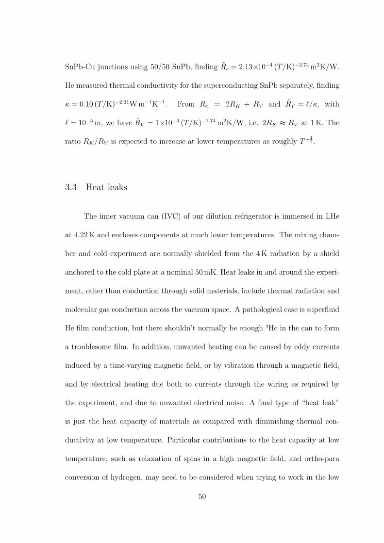
SnPb-Cu junctions using 50/50 SnPb, finding Rc = 2.13×10⁻⁴ (T/K)−2.74 m2K/W.
He measured thermal conductivity for the superconducting SnPb separately, finding
κ = 0.10 (T/K)−2.31W m−1K−1. From Rc = 2RK + RV and RV = ℓ/κ, with
ℓ = 10−5 m, we have RV = 1×10⁻⁴ (T/K)−2.74 m2K/W, i.e. 2RK ≈ RV at 1 K. The
ratio RK/RV is expected to increase at lower temperatures as roughly T− 1
2 .
3.3 Heat leaks
The inner vacuum can (IVC) of our dilution refrigerator is immersed in LHe
at 4.22 K and encloses components at much lower temperatures. The mixing cham-
ber and cold experiment are normally shielded from the 4 K radiation by a shield
anchored to the cold plate at a nominal 50 mK. Heat leaks in and around the experi-
ment, other than conduction through solid materials, include thermal radiation and
molecular gas conduction across the vacuum space. A pathological case is superfluid
He film conduction, but there shouldn’t normally be enough 4He in the can to form
a troublesome film. In addition, unwanted heating can be caused by eddy currents
induced by a time-varying magnetic field, or by vibration through a magnetic field,
and by electrical heating due both to currents through the wiring as required by
the experiment, and due to unwanted electrical noise. A final type of “heat leak”
is just the heat capacity of materials as compared with diminishing thermal con-
ductivity at low temperature. Particular contributions to the heat capacity at low
temperature, such as relaxation of spins in a high magnetic field, and ortho-para
conversion of hydrogen, may need to be considered when trying to work in the low
50
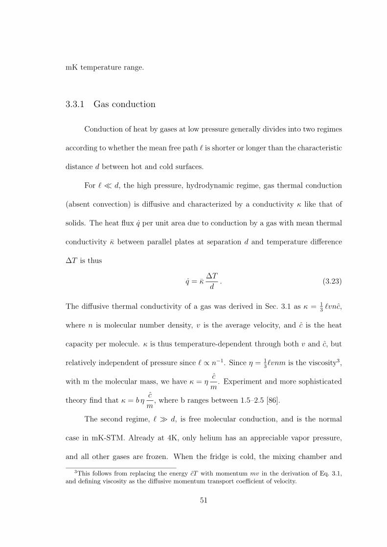
mK temperature range.
3.3.1 Gas conduction
Conduction of heat by gases at low pressure generally divides into two regimes
according to whether the mean free path ℓ is shorter or longer than the characteristic
distance d between hot and cold surfaces.
For ℓ ≪ d, the high pressure, hydrodynamic regime, gas thermal conduction
(absent convection) is diffusive and characterized by a conductivity κ like that of
solids. The heat flux q per unit area due to conduction by a gas with mean thermal
conductivity κ between parallel plates at separation d and temperature difference
∆T is thus
q = κ∆T
d. (3.23)
The diffusive thermal conductivity of a gas was derived in Sec. 3.1 as κ = 1
3ℓvnc,
where n is molecular number density, v is the average velocity, and c is the heat
capacity per molecule. κ is thus temperature-dependent through both v and c, but
relatively independent of pressure since ℓ ∝ n−1. Since η = 1
3ℓvnm is the viscosity3,
with m the molecular mass, we have κ = ηc
m. Experiment and more sophisticated
theory find that κ = b ηc
m, where b ranges between 1.5–2.5 [86].
The second regime, ℓ ≫ d, is free molecular conduction, and is the normal
case in mK-STM. Already at 4K, only helium has an appreciable vapor pressure,
and all other gases are frozen. When the fridge is cold, the mixing chamber and
3This follows from replacing the energy cT with momentum mv in the derivation of Eq. 3.1,and defining viscosity as the diffusive momentum transport coefficient of velocity.
51
other components at millikelvin temperatures will pump any He down to the vapor
pressure for the coldest surface temperatures present. One symptom of a He leak
into the IVC is periodic spikes in temperature at the mixing chamber. He condenses
on the cold parts, forming droplets and dripping down onto the warmer shield or
the 4 K IVC. Each drop becomes a sudden burst of warm gas which condenses again
on the cold parts. Whether this occurs is controlled by the total amount of helium
left in the IVC. We use 3He as exchange gas, which needs to be pumped out at
4 K. The vapor pressure of 3He is about 3 times higher than that (1 bar) of 4He at
4.22 K, yet it still takes many hours to pump down to pressures compatible with
fridge operation.
Table 3.5 shows the approximate vapor pressures of 4He and 3He at 4 K and
lower temperatures. Also shown are values for ℓ calculated using [4]
ℓ = 28.7 µm
(
T
1 K
)1.147 (
p
1 Pa
)−1
, (3.24)
where p is pressure, and assuming T = 1 K (although the coldest components limit
p, the gas temperature in the vicinity of warmer components may be higher). For
comparison, the relevant dimension d for a mK-STM cryostat ranges from 1 mm to
10 cm.
Once the mixing chamber reaches 0.1 K or lower, the pressure of 3He can’t be
greater than 10−8 Pa [3], from which we calculate ℓ ≈ 3 km, i.e. well in the free
molecular regime. However, if the mixing chamber is as warm as 0.2 K, we find
p ≈ 10−2 Pa, and then ℓ ≈ 3mm, crossing into the diffusive regime. Of course, if we
raise the temperature in a dilution fridge this high, using a heater, we are probably
52
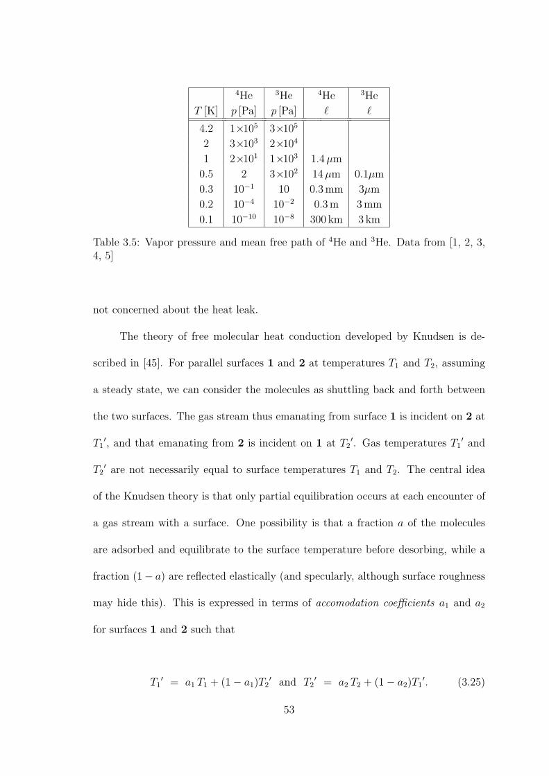
4He 3He 4He 3He
T [K] p [Pa] p [Pa] ℓ ℓ
4.2 1×10⁵ 3×10⁵
2 3×10³ 2×10⁴
1 2×101 1×10³ 1.4 µm
0.5 2 3×10² 14 µm 0.1µm
0.3 10−1 10 0.3 mm 3µm
0.2 10−4 10−2 0.3 m 3 mm
0.1 10−10 10−8 300 km 3 km
Table 3.5: Vapor pressure and mean free path of 4He and 3He. Data from [1, 2, 3,4, 5]
not concerned about the heat leak.
The theory of free molecular heat conduction developed by Knudsen is de-
scribed in [45]. For parallel surfaces 1 and 2 at temperatures T1 and T2, assuming
a steady state, we can consider the molecules as shuttling back and forth between
the two surfaces. The gas stream thus emanating from surface 1 is incident on 2 at
T1′, and that emanating from 2 is incident on 1 at T2
′. Gas temperatures T1′ and
T2′ are not necessarily equal to surface temperatures T1 and T2. The central idea
of the Knudsen theory is that only partial equilibration occurs at each encounter of
a gas stream with a surface. One possibility is that a fraction a of the molecules
are adsorbed and equilibrate to the surface temperature before desorbing, while a
fraction (1− a) are reflected elastically (and specularly, although surface roughness
may hide this). This is expressed in terms of accomodation coefficients a1 and a2
for surfaces 1 and 2 such that
T1′ = a1 T1 + (1 − a1)T2
′ and T2′ = a2 T2 + (1 − a2)T1
′. (3.25)
53
Solving these equations, we find that
T1′ =
a1T1 + a2(1 − a1)T2
a1 + a2 − a1a2
, T2′ =
a2T2 + a1(1 − a2)T1
a1 + a2 − a1a2
, (3.26)
and T1′ − T2
′ =a1 a2
a1 + a2 − a1a2
(T2 − T1)
≡ G · (T1 − T2) . (3.27)
The heat flux from surface 1 to 2 per unit area is then given by [45, 86]
q =1
4G
γ + 1
γ − 1
√
2R
πMp
T1 − T2√T
(3.28)
where γ is the heat capacity ratio Cp/Cv, which has the value 5
3for He, R is the
molar gas constant 8.3 J K−1mol−1, M is the molar mass (3 or 4 ×10⁻³ kg mol−1
for He), p is pressure, and T is an effective gas temperature such that (for parallel
surfaces)
1√T
=1
2
( 1√
T1′+
1√
T2′
)
. (3.29)
For nested surfaces of substantially differing areas, T will be weighted toward the
temperature of the outer surface. The factor G = a1a2/(a1 + a2 − a1a2) can also be
modified for such geometries (see below).
Unfortunately, accomodation coefficients a are not well characterized for many
surfaces, gases and temperatures. For He on very clean metal surfaces, a can be as
low as ∼10−2, but for most cases a > 0.2 [45, 87]. For estimation purposes, one can
use a ≈ 1
2and simplify Eq. 3.28 to
q = b · p
1 Pa· (T2 − T1)√
T · 1 K· W
m2, (3.30)
where the constant b takes the approximate values 14 for 3He and 12 for 4He.
54
3.3.2 Radiation
The heat of thermal electromagnetic radiation from a surface is given by the
Stefan-Boltzmann equation,
q = ǫ σ T 4, (3.31)
where q is the radiated power per unit area, σ = 5.67×10⁻⁸W
m2K4is the Stefan-
Boltzmann constant, and emissivity ǫ is a property of the surface whose value can
range between close to unity for a “black body” and as low as about 10−2 for highly
polished metal surfaces [86]. Emissivity is related to reflectivity R by ǫ = (1 − R).
Since R, defined as the ratio of reflected to incident power, is a function of wave-
length, ǫ as defined by Eq. 3.31 is necessarily a function of temperature.
For the simplest case, two parallel surfaces of equal emissivity ǫ, at tempera-
tures T1 and T2 ≤ T1, the net heat flux per unit area is
q = σG (T 41 − T 4
2 ) (3.32)
where G is the geometric factor (Sec. 3.3.3) which in this case is G =ǫ
2 − ǫ.
Classical theory and some books [4] predict that emissivity scales as the square
root of resistivity ρ according to ǫ = 0.365
√
ρ
λ·1 Ω, but for pure metals with low
residual resistivity, at low temperature the reflectivity is limited by the anomalous
skin effect [88, 86], and ǫ for even highly polished cold metal surfaces is typically
not smaller than ∼10−2.
The spectrum of black body radiation has a peak in wavelength at
λmax = 2.9 mm · 1 K
T, (3.33)
55
known as Wien’s law [86]. For most materials at most temperatures, this gives a
useful estimate of wavelength for most of the radiated power. Thus, for example,
at 50 mK, the nominal temperature of the radiation shield surrounding the mixing
chamber plate and experimental volume of our dilution fridge, λmax ≃ 6 cm. The
wavelength is long enough to interact with the geometry of parts and affect radiative
heat transfer at this temperature.
Wien’s law is typically quoted for the wavelength domain. However, since
dλ = − c
f 2df , the power spectral density in the frequency (or energy) domain peaks
at a slightly different value, with fmax ≈ 59 T GHz/K. Thus at 50 mK, fmax ≈ 3 GHz.
3.3.3 Geometrical factors
Heat leaks between exposed surfaces in the vacuum space of a cryostat are
due to two mechanisms, radiation and gas conduction in the free molecular regime.
Both involve the random emission and reflection, or absorption and re-emission, of
energy carriers. Accomodation coefficients and emissivities are analogous in that
they quantify the fractional equilibration of the energy stream in each encounter
with a surface. This leads to similar geometric factors.
The easiest cases to model are those in which one surface completely encloses
the other. In a cryostat typically an enclosed surface 2 will be colder than surface 1
enclosing it. For geometries such as concentric cylinders or spheres, the probability
that a photon emitted from the enclosing surface 1 hits the enclosed surface 2 is
estimated by the area ratio A =A2
A1
where A2 and A1 are the areas of the two
56
surfaces. The fraction of the flux emitted by 1 that is absorbed by 2 is then Aǫ2
and the fraction that returns to 1 is 1 − Aǫ2. Only a fraction ǫ1 of the returning
flux is absorbed while 1− ǫ1 of it is reflected, and Aǫ2 of that is absorbed by 1, etc.
Therefore if σ A1 ǫ1 T 41 is the total flux emitted by the enclosing surface 1, and
if we define x ≡ (1−Aǫ2)(1−ǫ1) as the factor by which the reflection of the reflection
is diminished, we have the total power absorbed by the enclosed surface 2 as
Q1 = Aǫ2 × σA1 ǫ1 T 41 × [1 + x + x2 + ...] = σA2 T 4
1 ǫ1ǫ2
1
1 − x. (3.34)
Similarly, the total flux emitted by 2 is σA2ǫ2T42 , and that absorbed by 1 is
σA2ǫ2T42
1
1 − xǫ1. Hence the net heat transferred from 1 to 2 is
Q = σ A2 G (T 41 − T 4
2 ), (3.35)
where we have defined
G ≡ ǫ1ǫ2
1 − x=
ǫ1ǫ2
1 − (1 − Aǫ1)(1 − ǫ2)=
ǫ1ǫ2
ǫ2 + Aǫ1(1 − ǫ2)(3.36)
By replacing emissivities ǫi with accomodation coefficients ai in Eq. 3.36, we
have the geometrical factor for molecular gas conduction.
This formula for G was derived under the assumption of no correlation be-
tween the direction of reflected radiation and its source, i.e. that each “bounce”
is independent and the probability of hitting the inner surface is subject to the
same area factor each time. This is true for diffuse reflection or for desorbtion of
molecules. It is not true for specular reflection with a geometry, such as concentric
surfaces, such that a ray that has transited between two surfaces is likely aligned to
57
continue bouncing between the two. In this case, the area ratio A can be taken out
of the formula for G.
These calculations can in general provide only rough estimates of heat, partic-
ularly for mK temperatures. The geometries are idealized, and the formulas ignore
such factors as the dependence of ǫ on temperature and wavelength, or the effect
of electromagnetics and geometry when thermal peak wavelengths are the size of
cryostat parts.
3.3.4 Shields
Another important geometry is that of n “floating” parallel planar shields
interposed between parallel surfaces S0 and Sn+1 at temperatures T0 and Tn+1 < T0.
Here “floating” means that the heat fluxes in and out of an area element via vacuum
heat leaks are large in comparison to any solid-solid thermal contact. Such shields
are typically metallic, but need not be.
Assume that there is no significant leakage into, out of, or across (“short-
circuiting”) the system of shields. Further, assume that the temperature on both
sides of one shield is the same. For each pair of facing surfaces assume that the net
heat transfer is the sum of fluxes in each direction, each of which is the same function
of the temperature of the emitting surface only (taking into account emissivities and
multiple reflections). This would be the case, for example, if all the surfaces are
similar.
If Qk is the heat flux from a surface at temperature Tk, and T1 . . . Tn are
58
the temperatures of the shields, then energy conservation requires in the steady
state that Qk−1 − Qk = Qk − Qk+1 for 1 ≤ k ≤ n. It follows directly that
Qn+1 − Q0 = n(Qk − Qk−1), i.e. the net heat flux through the system of shields is
1
nof what it would be without them.
Although many books derive this principle by invoking the Stefan-Boltzmann
law [89], as seen here the result is more general and should be valid not only for
radiation but also approximately for molecular conduction. For radiation, the con-
dition ∆T 4 = const. for the temperature steps leads to T 3∆T ≈ const., so that the
largest steps in absolute temperature occur between the lowest temperatures. When
molecular conduction is important, the steps will be closer to ∆T = const..
Interposing “floating” shields will not be effective in the case of diffusive con-
duction, but thermally anchored shields may still be useful to intercept the vacuum
heat leaks and create a cold environment.
3.3.5 Example calculation: Heat transfer to 50mK shield
As an example, we can consider the vacuum heat leaks to the radiation shield
surrounding the mixing chamber and experimental volume of our dilution refriger-
ator. This shield is thermally anchored to a point along the heat exchanger line
between the still and mixing chamber which is expected to be at ∼50 mK. It con-
sists of a copper cylinder 159 mm in diameter and 211 mm long with a cylindrical
tailpiece 67 mm in diameter and 457 mm long. It fits snugly inside the stainless steel
IVC with a 3–5 mm gap. Although the geometry is nested cylinders, they are close
59
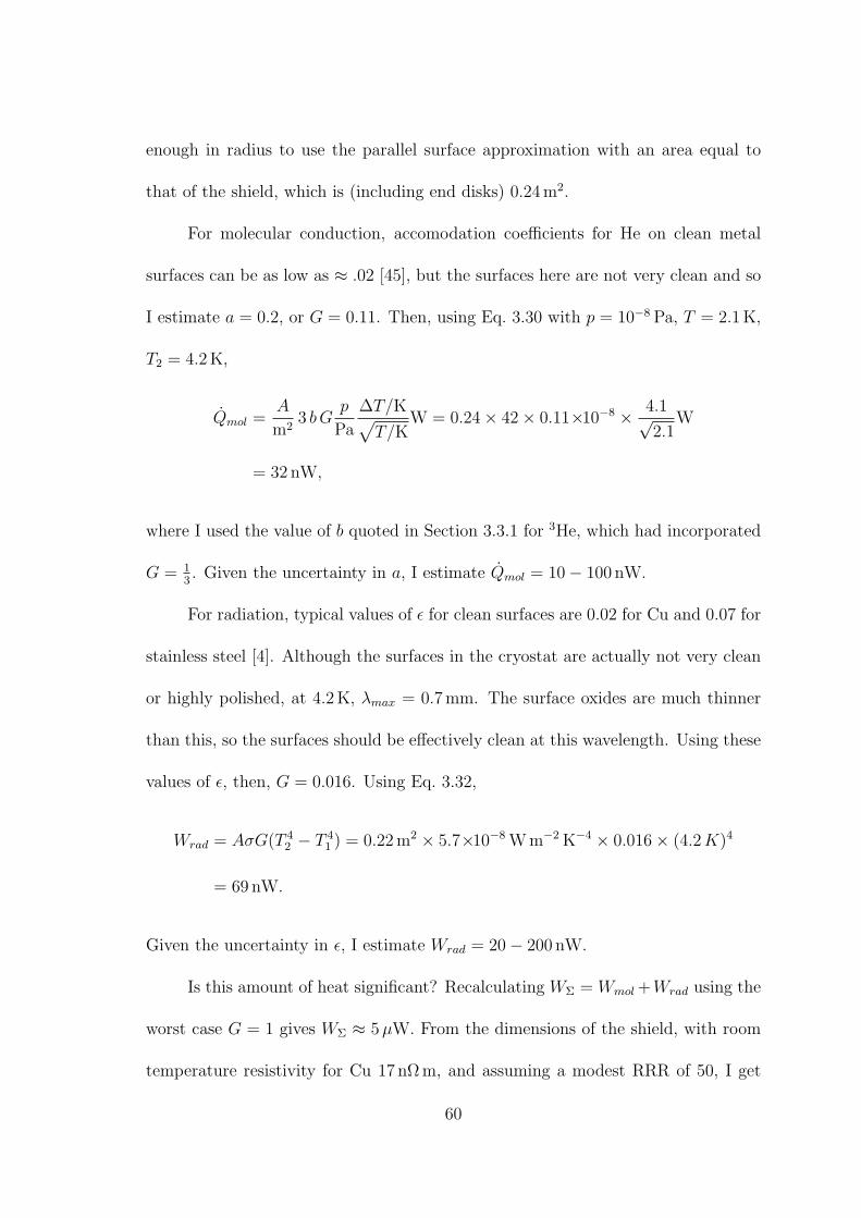
enough in radius to use the parallel surface approximation with an area equal to
that of the shield, which is (including end disks) 0.24 m2.
For molecular conduction, accomodation coefficients for He on clean metal
surfaces can be as low as ≈ .02 [45], but the surfaces here are not very clean and so
I estimate a = 0.2, or G = 0.11. Then, using Eq. 3.30 with p = 10−8 Pa, T = 2.1 K,
T2 = 4.2 K,
Qmol =A
m23 bG
p
Pa
∆T/K√
T/KW = 0.24 × 42 × 0.11×10−8 × 4.1√
2.1W
= 32 nW,
where I used the value of b quoted in Section 3.3.1 for 3He, which had incorporated
G = 1
3. Given the uncertainty in a, I estimate Qmol = 10 − 100 nW.
For radiation, typical values of ǫ for clean surfaces are 0.02 for Cu and 0.07 for
stainless steel [4]. Although the surfaces in the cryostat are actually not very clean
or highly polished, at 4.2 K, λmax = 0.7 mm. The surface oxides are much thinner
than this, so the surfaces should be effectively clean at this wavelength. Using these
values of ǫ, then, G = 0.016. Using Eq. 3.32,
Wrad = AσG(T 42 − T 4
1 ) = 0.22 m2 × 5.7×10−8 W m−2 K−4 × 0.016 × (4.2 K)4
= 69 nW.
Given the uncertainty in ǫ, I estimate Wrad = 20 − 200 nW.
Is this amount of heat significant? Recalculating WΣ = Wmol +Wrad using the
worst case G = 1 gives WΣ ≈ 5 µW. From the dimensions of the shield, with room
temperature resistivity for Cu 17 nΩ m, and assuming a modest RRR of 50, I get
60
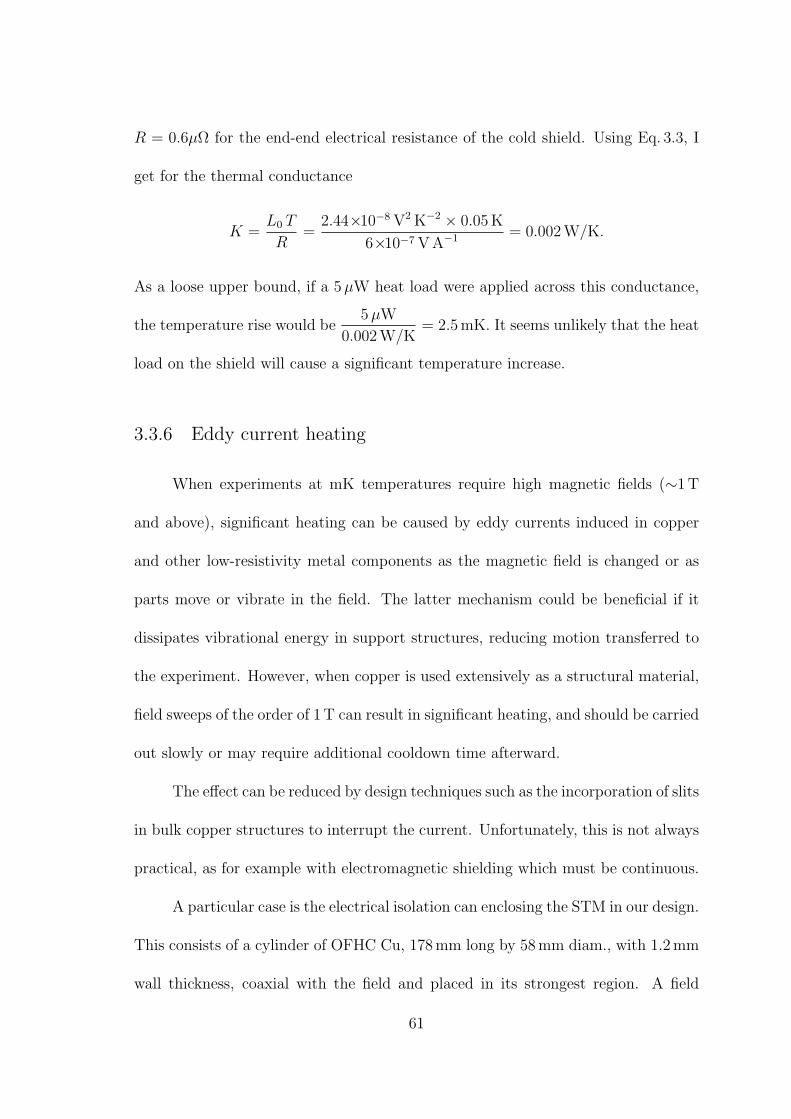
R = 0.6µΩ for the end-end electrical resistance of the cold shield. Using Eq. 3.3, I
get for the thermal conductance
K =L0 T
R=
2.44×10⁻⁸ V2 K−2 × 0.05 K
6×10⁻⁷ V A−1= 0.002 W/K.
As a loose upper bound, if a 5µW heat load were applied across this conductance,
the temperature rise would be5 µW
0.002 W/K= 2.5 mK. It seems unlikely that the heat
load on the shield will cause a significant temperature increase.
3.3.6 Eddy current heating
When experiments at mK temperatures require high magnetic fields (∼1 T
and above), significant heating can be caused by eddy currents induced in copper
and other low-resistivity metal components as the magnetic field is changed or as
parts move or vibrate in the field. The latter mechanism could be beneficial if it
dissipates vibrational energy in support structures, reducing motion transferred to
the experiment. However, when copper is used extensively as a structural material,
field sweeps of the order of 1 T can result in significant heating, and should be carried
out slowly or may require additional cooldown time afterward.
The effect can be reduced by design techniques such as the incorporation of slits
in bulk copper structures to interrupt the current. Unfortunately, this is not always
practical, as for example with electromagnetic shielding which must be continuous.
A particular case is the electrical isolation can enclosing the STM in our design.
This consists of a cylinder of OFHC Cu, 178 mm long by 58 mm diam., with 1.2 mm
wall thickness, coaxial with the field and placed in its strongest region. A field
61
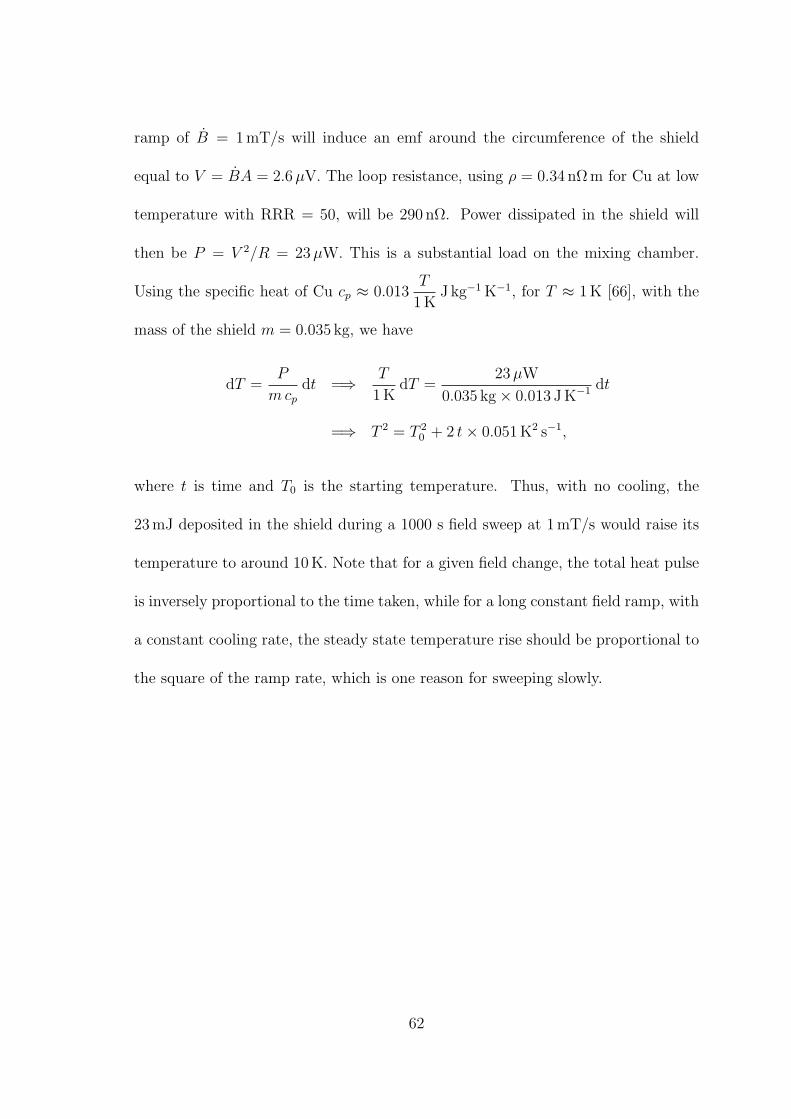
ramp of B = 1 mT/s will induce an emf around the circumference of the shield
equal to V = BA = 2.6 µV. The loop resistance, using ρ = 0.34 nΩ m for Cu at low
temperature with RRR = 50, will be 290 nΩ. Power dissipated in the shield will
then be P = V 2/R = 23 µW. This is a substantial load on the mixing chamber.
Using the specific heat of Cu cp ≈ 0.013T
1 KJ kg−1 K−1, for T ≈ 1 K [66], with the
mass of the shield m = 0.035 kg, we have
dT =P
m cp
dt =⇒ T
1 KdT =
23 µW
0.035 kg × 0.013 J K−1dt
=⇒ T 2 = T 20 + 2 t × 0.051 K2 s−1,
where t is time and T0 is the starting temperature. Thus, with no cooling, the
23 mJ deposited in the shield during a 1000 s field sweep at 1 mT/s would raise its
temperature to around 10 K. Note that for a given field change, the total heat pulse
is inversely proportional to the time taken, while for a long constant field ramp, with
a constant cooling rate, the steady state temperature rise should be proportional to
the square of the ramp rate, which is one reason for sweeping slowly.
62
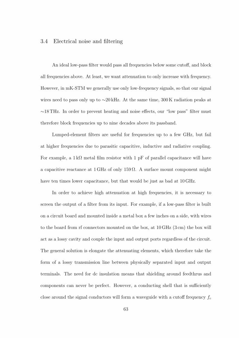
3.4 Electrical noise and filtering
An ideal low-pass filter would pass all frequencies below some cutoff, and block
all frequencies above. At least, we want attenuation to only increase with frequency.
However, in mK-STM we generally use only low-frequency signals, so that our signal
wires need to pass only up to ∼20 kHz. At the same time, 300 K radiation peaks at
∼18 THz. In order to prevent heating and noise effects, our “low pass” filter must
therefore block frequencies up to nine decades above its passband.
Lumped-element filters are useful for frequencies up to a few GHz, but fail
at higher frequencies due to parasitic capacitive, inductive and radiative coupling.
For example, a 1 kΩ metal film resistor with 1 pF of parallel capacitance will have
a capacitive reactance at 1 GHz of only 159 Ω. A surface mount component might
have ten times lower capacitance, but that would be just as bad at 10 GHz.
In order to achieve high attenuation at high frequencies, it is necessary to
screen the output of a filter from its input. For example, if a low-pass filter is built
on a circuit board and mounted inside a metal box a few inches on a side, with wires
to the board from rf connectors mounted on the box, at 10 GHz (3 cm) the box will
act as a lossy cavity and couple the input and output ports regardless of the circuit.
The general solution is elongate the attenuating elements, which therefore take the
form of a lossy transmission line between physically separated input and output
terminals. The need for dc insulation means that shielding around feedthrus and
components can never be perfect. However, a conducting shell that is sufficiently
close around the signal conductors will form a waveguide with a cutoff frequency fc
63
which can be set fairly high. For example, given a cylindrical coaxial geometry with
rinner/router = 0.5, the cutoff wavelength for the lowest mode is λc ≈ 2 rinner [90], so
we have
fc =c
2 rinner
√ǫ, (3.37)
with c the speed of light and ǫ the dielectric constant of the insulator. Thus for
rinner = 0.1 mm and ǫ = 10 we find fc ≈ 500 GHz. A waveguide cutoff above 100 GHz
is generally good enough since higher frequencies will be absorbed, reemitted and
thermalized along the length.
Lossy transmission lines can be based on dissipation in conductors or di-
electrics. Distributed RC filters use the capacitance of a shielded transmission line
with resistive conductors. Dissipative dielectrics include metals powders and ferro-
magnetic materials. These high-frequency loss mechanisms may be combined with
lumped-element RLC filtering to define the low-frequency cutoff, which may involve
separate filters built out of lumped-element components, or may take advantage of
the integral RLC characteristics of the lossy transmission line.
3.4.1 Dissipative dielectric filters
The metal powder filter, invented by Martinis, et al. [91], may be generalized
as a lossy transmission line in which the loss is due to electromagnetic interaction
with a medium which is dissipative at high frequencies and which fills the cavity
space between the conductor and the outer body. The conductor can be chosen for
low (or zero) dc resistance. Martinis used copper powder as a dissipative medium,
64
leading to this type of filter being commonly known as a “copper powder filter.”
However, other investigators [92, 93, 94, 95] have found alloys such as bronze and
stainless steel powders to be more effective at low temperatures. Recently, several
groups [96, 97] have reported the use of magnetic materials such as ferrite powders
in polymer matrix. The coupling is far stronger and provides far higher attenuation
per unit length, enabling long coiled wires to be replaced with short, impedance-
matched striplines.
In Martinis-style metal powder filters, the metal grains are typically 10-100µm
in size. The native oxide layer at the surface of each grain insulates to low voltages,
and microwave energy can penetrate into the metal powder matrix because it is
insulating on the scale of a wavelength. Within each metal grain, just below the oxide
layer, eddy currents are excited which act to cancel the electromagnetic field and
thus exclude it from the interior of the metal. These currents decay exponentially
into the bulk metal with a length scale δ called the skin depth. The total surface
current required to cancel the field is determined by the field intensity, therefore
applying W = I2R, the formula for power dissipation in a resistance R carrying a
current I, we expect that the power dissipation will be proportional to the ratio of
resistivity to skin depth,
w ∝ ρ
δ≡ Rs (3.38)
which defines the surface resistance Rs, where ρ the resistivity of the metal, and
δ =
√
ρ
πfµ(3.39)
65
is the skin depth4 at frequency f for a metal with magnetic permeability µ. For Cu
at room temperature, δ = 6.6 µm at 100 MHz [99].
An explicit calculation of power loss per unit area of a plane metal surface
subject to a tangential magnetic field H0e−2πift [100, 99] finds
w =1
2H2
0
√
πfµρ =1
2J2
s Rs (3.40)
in agreement with this argument. Here Js is the surface current and is equal in
magnitude to H0, the magnetic field intensity tangential to the surface. Since H0 is
locally varying over the surface of each grain as well as dependent on its location
and the overall geometry of a filter, it would be hard to use Eq. 3.40 to directly
calculate the total attenuation of a filter (also, the plane approximation would be
invalid at low frequencies). However, since we know that H20 ∝ Pin, where Pin is
power input to a filter, Eq. 3.40 tells us how power loss in the metal grains depends
on frequency, resistivity and permeability, assuming the skin depth is less than the
particle radius.
If we consider a filter as divided into n equally-constituted sections, taking the
limit as n → ∞, the power lost in each section is
Wk = PkαRs
n(3.41)
for some unknown coupling constant α ≪ R−1s , where Pk is the power input to
section k from section k − 1. By energy conservation, neglecting the possibility of
4The anomalous skin effect [98], which occurs at low temperatures when the mean free pathof electrons exceeds the classical skin depth, is not relevant here since powder filters typically uselow-purity or alloy metals.
66
reflection,
Pk+1 = Pk − Wk = Pk
(
1 − αRs
n
)
. (3.42)
Taking the limit, and defining β ≡ α√
π/ℓ, we obtain
Pout
Pin
= limn→∞
(
1 − αRs
n
)n
= exp(−αRs) ≡ exp(−βℓ√
fµρ ) (3.43)
as the functional form of the high-frequency attenuation for a filter of length ℓ. Note
that the definition of β serves to eliminate√
π and introduce ℓ, and the purpose of
Eq. 3.43 is just to show some of the dependence of the attenuation on some variables.
However, β will depend on details of the filter geomtery, particle size and density,
and other factors, possibly including some of the variables appearing in Eq. 3.43. In
the latter case, Eq. 3.43 will only approximate the dependence on these variables.
Equation 3.43 does not appear to have been reported in the literature on metal
powder filters. Usually such filters are made to have such high attenuation that they
hit the noise floor of typical network analyzers above about 1 GHz, making it hard to
measure the attenuation at high frequency. Also, the filters are subject to resonances
which can affect the attenuation curve where it is measurable.
Milliken et al. [94] observed apparent exponential behavior for their 50 Ω
straight-wire powder filters, or Pout/Pin ∝ exp(−f/fc). Their data are shown in
Fig. 3.1. In contrast, measurements of a coiled-wire powder filter made in our lab
(Fig. 5.4, Chapter 5) are consistent with Pout/Pin ∝ exp(−(f/fc)γ) with γ ≈ 0.63.
Both filters used similar (perhaps not identical) spherical, -325 mesh, 70/30 Cu/Sn
bronze powder, which Milliken et al. found to provide the best attenuation out of
several types they tested. Figure 3.1(A) shows an SEM image of the material, taken
67
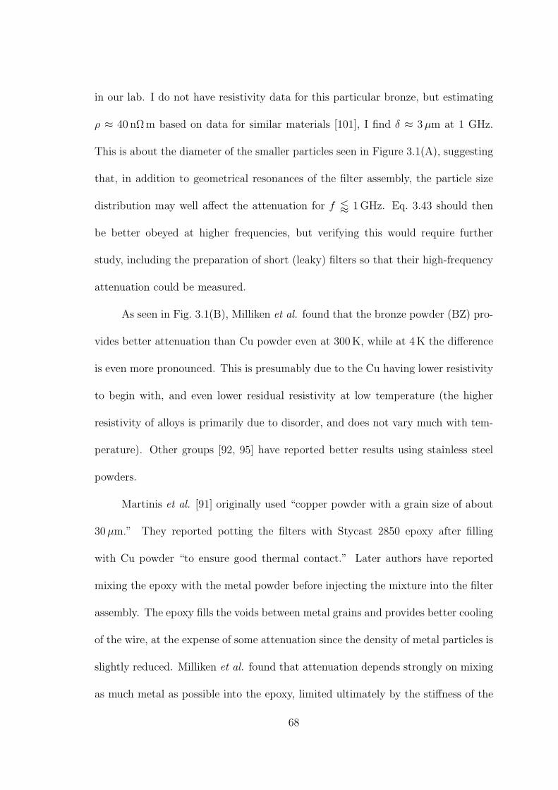
in our lab. I do not have resistivity data for this particular bronze, but estimating
ρ ≈ 40 nΩ m based on data for similar materials [101], I find δ ≈ 3 µm at 1 GHz.
This is about the diameter of the smaller particles seen in Figure 3.1(A), suggesting
that, in addition to geometrical resonances of the filter assembly, the particle size
distribution may well affect the attenuation for f / 1 GHz. Eq. 3.43 should then
be better obeyed at higher frequencies, but verifying this would require further
study, including the preparation of short (leaky) filters so that their high-frequency
attenuation could be measured.
As seen in Fig. 3.1(B), Milliken et al. found that the bronze powder (BZ) pro-
vides better attenuation than Cu powder even at 300 K, while at 4 K the difference
is even more pronounced. This is presumably due to the Cu having lower resistivity
to begin with, and even lower residual resistivity at low temperature (the higher
resistivity of alloys is primarily due to disorder, and does not vary much with tem-
perature). Other groups [92, 95] have reported better results using stainless steel
powders.
Martinis et al. [91] originally used “copper powder with a grain size of about
30µm.” They reported potting the filters with Stycast 2850 epoxy after filling
with Cu powder “to ensure good thermal contact.” Later authors have reported
mixing the epoxy with the metal powder before injecting the mixture into the filter
assembly. The epoxy fills the voids between metal grains and provides better cooling
of the wire, at the expense of some attenuation since the density of metal particles is
slightly reduced. Milliken et al. found that attenuation depends strongly on mixing
as much metal as possible into the epoxy, limited ultimately by the stiffness of the
68
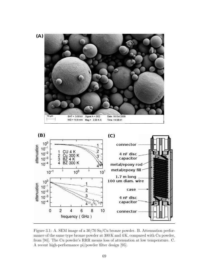
Figure 3.1: A. SEM image of a 30/70 Sn/Cu bronze powder. B. Attenuation perfor-mance of the same type bronze powder at 300 K and 4 K, compared with Cu powder,from [94]. The Cu powder’s RRR means loss of attenuation at low temperature. C.A recent high-performance pi/powder filter design [95].
69
resulting paste [94].
Stycast 2850FT is an epoxy filled with grains of an unreported but hard,
crystalline material. Its thermal conductivity in the mK range is not particularly
high: 9.2×( T
1 K
)2.65 mW
m·K [60, 55], four times lower at 1 K than the unfilled Stycast
1266, (which also exhibits a lower exponent, as expected for disordered polymers).
Popular legend claims the thermal contraction of 2850FT is matched to Cu, but in
fact its thermal contraction integral from 300 to 4 K,∆ℓ
ℓ= 0.44%, is higher than that
of Cu (0.324%) or of most metals, but much lower than pure epoxies (& 1 %). This
lower thermal contraction is the principal advantage of mixing the metal powder
with 2850FT instead of an unfilled epoxy. Otherwise, stresses developed during
thermal cycling can crack the metal/epoxy, potentially breaking the wire.
The relatively weak eddy current coupling of Martinis-style filters means that
typically 1–4 m of wire needs to pass through the metal powder to provide adequate
attenuation. The only practical way to do this in a filter of reasonable dimensions
is with tightly coiled fine wire. Copper wire is often used, or Cu-clad NbTi. Some
people fashion freestanding coils and then fill them with powder or metal/epoxy,
but this results in poor control of the geometry and characteristics. It is better
to wind the coils on pre-cast rods of metal/epoxy. Lukashenko and Ustinov [95]
have reported very reproducible, compact (∼1 in. length), high performance filters
using 0.1 mm diameter Cu wire wound on pre-cast rods with no space between turns
(Fig. 3.1). They add capacitors at either end, exploiting the inductance of the coil
to place an LC pi-filter effectively in series with the inductively-coupled microwave
dissipation.
70
Coiled-wire filters have large inductances and usually exhibit unwanted reso-
nances as well as creating a severe impedance mismatch. Milliken et al. developed
coaxial straight-wire filters with 50 Ω impedance, useful for wideband time-domain
measurements, but with 6 in. length these filters achieved only 20 dB of attenua-
tion at 2 GHz [94]. Martinis-style filters are mostly used for dc or low frequency
wiring, or for transmitting rf signals when multiple reflections and attenuation are
not problematic.
Another approach to filter construction is to start with a Minicircuits LC bar-
rel filter assembly [102]. These are available with a range of cutoff frequencies up to
around 1 GHz, and are engineered for 50 Ω impedance within their passband, with a
steep rolloff. Their attenuation drops at higher frequencies due to parasitic capac-
itances and transmission via the cavity space around components and conductors.
To reduce the latter, the barrel can be filled with metal/epoxy through holes drilled
in its side. About -70 dB of attenuation from 2-40 GHz has been achieved this way
using Cu powder mixed 50 % by weight with Stycast 1266 [103].
A recent development, at least in low-temperature physics, is the use of fer-
romagnetic or ferrimagnetic microwave absorbing materials, such as Eccosorb [104]
silicones and epoxies loaded with carbonyl iron or ferrite [96, 97]. These materials
are much stronger microwave absorbers than nonmagnetic metal powders, and can
provide adequate attenuation in filters constructed as short, impedance-matched
striplines. Eddy current losses are expected to be higher given the higher resistiv-
ity and permeability of these materials, and hysteresis losses may play a role also.
Carbonyl iron appears to be the better absorber above about 10GHz, while ferrites
71
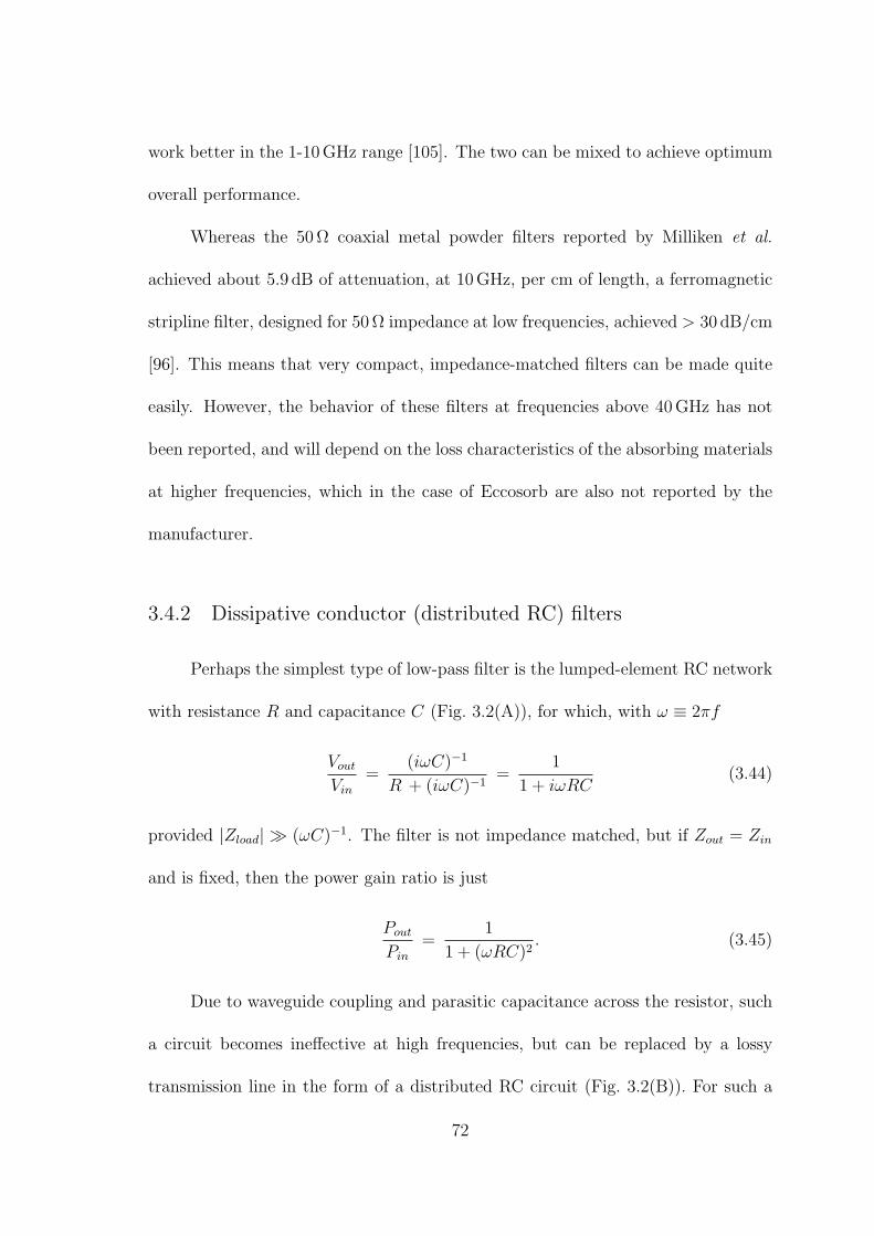
work better in the 1-10 GHz range [105]. The two can be mixed to achieve optimum
overall performance.
Whereas the 50 Ω coaxial metal powder filters reported by Milliken et al.
achieved about 5.9 dB of attenuation, at 10 GHz, per cm of length, a ferromagnetic
stripline filter, designed for 50 Ω impedance at low frequencies, achieved > 30 dB/cm
[96]. This means that very compact, impedance-matched filters can be made quite
easily. However, the behavior of these filters at frequencies above 40 GHz has not
been reported, and will depend on the loss characteristics of the absorbing materials
at higher frequencies, which in the case of Eccosorb are also not reported by the
manufacturer.
3.4.2 Dissipative conductor (distributed RC) filters
Perhaps the simplest type of low-pass filter is the lumped-element RC network
with resistance R and capacitance C (Fig. 3.2(A)), for which, with ω ≡ 2πf
Vout
Vin
=(iωC)−1
R + (iωC)−1=
1
1 + iωRC(3.44)
provided |Zload| ≫ (ωC)−1. The filter is not impedance matched, but if Zout = Zin
and is fixed, then the power gain ratio is just
Pout
Pin
=1
1 + (ωRC)2. (3.45)
Due to waveguide coupling and parasitic capacitance across the resistor, such
a circuit becomes ineffective at high frequencies, but can be replaced by a lossy
transmission line in the form of a distributed RC circuit (Fig. 3.2(B)). For such a
72
Figure 3.2: (A) Simple RC filter circuit; (B) Distributed RC filter circuit. C. Fre-quency dependence of Pout/Pin for RC filter ((1 + x2)−1, where x ≡ ωRC) anddistributed RC filter (exp(−
√2x)). D. Details of le Sueur’s [106] design for micro-
fabricated DRC filters, showing the chip layout, meander cross section, and housing.
73
line, neglecting inductance (which is not generally valid), the complex propagation
constant γ is [99]
γ =√
iωRC/ℓ2 (3.46)
where R and C are the total resistance and capacitance, and ℓ the total length. The
voltage attenuation constant per unit length is α = Re(γ) [99], i.e.
Pout
Pin
= exp(−2αℓ) = exp(−√
2ωRC). (3.47)
Comparing Eqs. 3.45 and 3.47 (Fig. 3.2) shows that, in the high-frequency
limit, the distributed RC is more effective than the lumped RC circuit of the same
total resistance and capacitance, even without considering parasitic reactances and
stray coupling.
One of the attractions of distributed RC filters is that, provided the shielding
is tight enough to prevent leakage or propagation down its length (up to some
waveguide cutoff which in general can be set quite high), this type of filter does
not suffer from the resonances at low frequencies and loss of attenuation at very
high frequencies (& 100 GHz) that affect metal powder filters. Attenuation is only
expected to increase with frequency, since the loss mechanism is just the resistance of
the conductors combined with the capacitance between them. The surface resistance
of the conductors only increases with frequency due to the skin effect, not accounted
for in Eq. 3.47), while the dielectric constant ǫ, and hence the capacitance, may vary
with frequency, but is bounded below by ǫ ≥ 1.
Vion et al. [107] introduced distributed RC filters to the literature on single
electron devices, in the form of a resistive meander line microfabricated on a chip.
74
They used an oxidized Si chip as substrate, deposited an Au ground plane, Si3N4
insulating layer, and AuCu meander with 1.5 kΩ total resistance and 20 pF total
capacitance to ground. They topped this with another Si3N4 insulating layer, and
mounted the chip in a close-fitting housing with SMA connectors. An indium seal
across the top of the insulated meander line served to reduce stray coupling of the
input and output terminals. However, successive folds of the meander line were not
shielded from each other. Courtois et al. [108] described similar filters, using CuNi
meander and straight lines deposited directly on a Cu block with a spun-on PPQ
(polyphenylquinoxaline) resist layer as insulator.
Le Sueur and Joyez [106, 109] developed an improved method for microfabri-
cated RC filter construction (Fig. 3.2), depositing AuCu on a brass substrate with
BCB (benzocyclobutene) photoresist as a dielectric. They insulated the top of the
meander with BCB and stripped the dielectric between folds so that an Au layer,
deposited on top of the insulator, contacted the brass substrate between folds to
form a shield all the way around the meander line, shielding each fold from the next
and ensuring a very high waveguide cutoff. Alternating narrow and wide sections
of the meander also served to increase reflection at high frequencies, a technique
known as stepped-impedance filtering [110].
The resulting filters are compact (∼1 cm3), have total resistance 77 Ω and ca-
pacitance 80 pF. Two were used in each line of le Sueur’s mK-STS system, one at
4 K and one at 30 mK. 25-line filter banks, and pair filters with triaxial connectors
for twisted-pair wiring, were also made. An important advantage of these micro-
fabricated RC filters is that, due to the thinness of the dielectric, and the use of
75
AuCu, a normal metal with low thermal contact resistance, the filters provide good
thermal grounding for the wires.
Another popular form of distributed RC filter, introduced by Zorin [90], is
based on Thermocoax [111], a resistive coaxial cable normally intended for use as a
high-temperature heating element.
Although these cables are available in a range of sizes with different materials,
for this purpose the best choice is the smallest diameter, 0.5 mm, with 304L stainless
steel shield. The center conductor is 80/20 NiCr, and the dielectric is tightly packed,
powdered MgO. The capacitance is high, 490 pF/m, and the dc resistance of the
inner conductor is 50 Ω/m. At high frequencies the resistance is enhanced by the
skin effect. To account for this, R in Eq. 3.47 can be replaced by
Reffective =ℓ
2πr1
Rs =ℓ
2πr1
√
πfµρ , (3.48)
where r1 is the radius of the inner conductor. By Zorin’s estimate, cutoff for the
lowest waveguide mode is above 0.5 THz. Higher frequencies are still strongly at-
tenuated by the resistive conductors and will thermalize along the length of the
cable. Thus, Thermocoax filters exhibit a smooth rolloff and reliable high frequency
attenuation.
Drawbacks of Thermocoax include the difficulty of cutting the shield to expose
the inner conductor without breaking it, and of soldering NiCr and SS304, which re-
quires the use of acid flux which can cause corrosion and electrical leakage. The MgO
powder is hygroscopic and develops significant leakage at room temperature when it
has aborbed moisture (let alone acid). The leakage current is noisy (Sec. 5.2.6) and
76
progressively worsens when leakage currents are allowed to flow at high voltage, so
that if Thermocoax is used with high-voltage lines, room temperature testing may
lead to a permanent failure. Therefore it is necessary to keep the Thermocoax dry
during assembly and to seal finished cables in order to keep water out.
Another issue is thermalization of Thermocoax cable at low temperature. Min-
eral powders (dry and in vacuum) have sometimes been used for cryostat (thermal)
insulation [89]. As shown in Sec. 3.5.4, the radial thermal conductance kr of the
insulation of 0.5 mm diameter Thermocoax at low temperature may be estimated as
kr . 2.3×10⁻³ (T/K)3 W m−1K−1. For Thermocoax with its shield anchored at
30 mK, this implies a 10 mK temperature rise for P . 6×10⁻¹⁰ W/m of Joule heat-
ing, or a current of I =√
P/49 Ωm−1 . 3.6 µA. Thus, at the lowest temperatures,
even small currents can cause significant heating of Thermocoax filters.
However, as also shown in Sec. 3.5.4, the length of Thermocoax that is required
to be anchored at low temperature in order for the inner conductor to thermalize is
not necessarily long. I estimate that two 1/e thermalization lengths at 30 mK would
be ∼3 cm.
Finally, a relatively new type of distributed RC filter uses twisted pairs of
normal or superconducting wire inside a close-fitting shield. Cu foil tape is used
for the shield, and by pressing many parallel twisted pairs between pieces of the
tape, multi-pair ribbons can be prepared. This type of filter offers the advantages
of integrating the filter function into the length of the wiring and of not requiring
that the inductive pickup immunity of twisted pairs be sacrificed in order to run the
conductors through separate filters.
77
Spietz et al [112] reported using 100µm diameter manganin wire pairs with Cu
adhesive tape folded in thirds over up to “10s” of the pairs at once. After folding
the tape over the pairs, they used a “rolling pin” (presumably rubber) to press
it into a form-fitting cover over the pairs, ensuring good shielding and relatively
high capacitance, 200 pF/m to the shield and 51 pF/m between the conductors.
Together with the inductance and resistance of the wire pairs, they achieved in the
neighborhood of 60 dB/m of attenuation at 1–40 GHz.
Bluhm et al [113] improved on this concept with the use of custom wire consist-
ing of 200µm OD CuNi with a 50µm diameter NbTi core. At microwave frequencies
the skin effect forces the current into the resistive outer shell of CuNi, providing high
attenuation with zero dc resistance.
3.5 Thermalization of wiring
3.5.1 Thermalization of a coaxial cable
At millikelvin temperatures the thermal conductivity of most insulators is
orders of magnitude lower than that of even highly resistive normal metals. Thus
the outer shield of a coaxial cable coming from a higher temperature may need to be
in contact with a thermal anchor for a considerable length at a lower temperature
in order for the inner wire to thermalize.
Heat flow in the coax can be modeled (Fig. 3.3) by axial heat conductances Kw
and Ks for the wire and shield, and a radial heat conductance through the dielectric
kd per unit length of the coax. I assume that the temperatures Tw and Ts of the wire
78
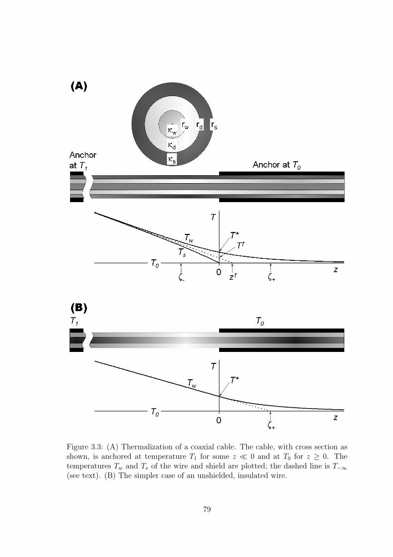
Figure 3.3: (A) Thermalization of a coaxial cable. The cable, with cross section asshown, is anchored at temperature T1 for some z ≪ 0 and at T0 for z ≥ 0. Thetemperatures Tw and Ts of the wire and shield are plotted; the dashed line is T−∞
(see text). (B) The simpler case of an unshielded, insulated wire.
79
and shield are functions of the axial dimension z only, whereas the temperature of
the dielectric Td is a function of both z and radius r. Also, I neglect the dependence
of thermal conductivity on temperature, and assume constant conductivities which
are the values at some mean temperature within the range of z in which the model
operates; the results will clarify the conditions under which this approximation is
valid.
The heats conducted axially by the wire and shield, Qw and Qs are given by
Qw = −KwdTw
dz, and Qs = −Ks
dTs
dz. (3.49)
With rw, rd, and rs the outer radii and κw, κd and κs the thermal conductivities of
the wire, dielectric, and shield materials,
Kw = π r2w κw , and Ks = π(r2
s − r2d) κs . (3.50)
If qr is the total radial heat per unit length, we can write
∂Td
∂r=
qr
2πrκd
=⇒ Td(r, z) =qr
2πκd
ln(r) + C . (3.51)
If thermal contact resistance (Sec. 3.2) is a significant factor, there will be a jump in
temperature at the inner and outer surfaces of the dielectric, given by
∆T = qrRc(2πr)−1, where Rc is the area-independent thermal contact resistivity. In
principle, Rc could be different for the wire-dielectric and shield-dielectric interfaces,
so using Rwdc and Rsd
c to distinguish these cases, we have
Ts = Tw + qr · kr , where
kr ≡[
Rwdc + Rd + Rsd
c
]−1
≡[
Rwdc
2πrw
+ln(rd/rw)
2πκd
+Rsd
c
2πrd
]−1
. (3.52)
80
To construct a simple model predicting Tw(z) and Ts(z), I assume (Fig. 3.3)
that the shield is in contact with the anchor at temperature T0 for z ≥ 0. Thus, for
all z ≥ 0, Ts = T0. I define T ∗ ≡ Tw(0) > T0, while for z → +∞, Tw → T0. Energy
conservation demands that, for z > 0,
dQw
dz= −qr , (3.53)
whence, applying Eqs. 3.49 and 3.52,
Kwd2Tw
dz2= (Tw − T0) kr , (3.54)
whence
d2Tw
dz2=
Tw − T0
ζ2+
, where ζ+ ≡√
Kw
kr
. (3.55)
Solving, for z ≥ 0,
Tw = T0 + (T ∗ − T0) exp(−z/ζ+). (3.56)
For z → −∞, Tw → T−∞ and Ts → T−∞, where
T−∞(z) ≡ T † + τ |z| . (3.57)
Here T † is a (so far) unknown temperature between T0 and T ∗, and τ ≡ limz→−∞
∣
∣
∣
∣
dTs
dz
∣
∣
∣
∣
is the temperature gradient for z ≪ 0. Note that Q ≡ τ (Kw + Ks) is the total heat
conducted along the coax from the higher to the lower temperature stage. Energy
conservation demands that, for all z < 0, Q = Qw + Qs, and that
dQw
dz= −qr = −dQs
dz. (3.58)
Applying Eqs. 3.49 and 3.52,
Kwd2Tw
dz2= kr (Tw − Ts) = −Ks
d2Ts
dz2, (3.59)
81
and combining terms,
d2(Tw − Ts)
dz2=
Tw − Ts
ζ2−
, (3.60)
where, defining η ≡ Kw
Ks
,
ζ− ≡√
Kw Ks
kr(Kw + Ks)= ζ+(1 + η)−
1
2 . (3.61)
Solving, for z ≤ 0,
Tw − Ts = (T ∗ − T0) exp(−|z|/ζ−) . (3.62)
Noting that the second derivative of T−∞ (Eq. 3.57) is zero, and applying
Eq. 3.59, I infer that, for z ≤ 0,
Tw = T † + τ |z| +1
1 + η(T ∗ − T0) exp(−|z|/ζ−)
Ts = T † + τ |z| − η
1 + η(T ∗ − T0) exp(−|z|/ζ−) . (3.63)
To find T ∗, I apply the continuity ofdTw
dz(energy conservation) at z = 0 :
dTw
dz
∣
∣
∣
∣
z=0−
= −τ +1
1 + η
T ∗ − T0
ζ−= −τ +
T ∗ − T0
ζ+
√1 + η
=dTw
dz
∣
∣
∣
∣
z=0+
= −T ∗ − T0
ζ+
; (3.64)
whence
T ∗ − T0 =τ
1
ζ+
+1
1 + η· 1
ζ−
=τ ζ+
1 + (1 + η)−1
2
. (3.65)
To find T †, in Eq. 3.63 I set z = 0 and Ts(0) = T0, obtaining
T † − T0 = (T ∗ − T0)η
1 + η, (3.66)
82
and applying Eq. 3.65,
T † − T0 =τ ζ+
1 + (1 + η)−1
2
· η
1 + η=
τ ζ+
1 + η +√
1 + η
= τ ζ+
[
1 − (1 + η)−1
2
]
= τ [ζ+ − ζ−] (3.67)
Finally, τ is generally not known directly, but rather, a section of coax of length
ℓ stretches between the anchor at T0 and another anchor at temperature T1 > T0.
If ℓ ≫ ζ−, a condition for the validity of this model, then
τ =T1 − T0
ℓ + z†, (3.68)
where z† is the T0 intercept of the T−∞ line (Fig. 3.3). Clearly,
z† =T † − T0
τ, (3.69)
and using Eqs. 3.66 and 3.65,
T † − T0 = (T ∗ − T0)η
1 + η=
τ ζ+
1 + (1 + η)−1
2
· η
1 + η. (3.70)
Therefore,
z† =ζ+ η
1 + η +√
1 + η= ζ+
[
1 − (1 + η)−1
2
]
= ζ+ − ζ−. (3.71)
Collecting and rewriting the results, defining α ≡ √1 + η =
√
1 + Kw/Ks,
and ζ ≡ ζ+ =√
Kw/kr, for z ≤ 0,
Tw = T0 + τ
[
|z| + ζ
1 − 1
α+
1
α(1 + α)exp
(
− α|z|ζ
)
]
Ts = T0 + τ
[
|z| + ζ
1 − 1
α−
(
1 − 1
α
)
exp(
− α|z|ζ
)
]
, (3.72)
83
and for z ≥ 0,
Tw = T0 + τζ
1 + α−1exp
(
− z
ζ
)
Ts = T0 . (3.73)
For practical purposes, the most useful of these results is the thermalization
length ζ. One might have written this down directly, but working out the model
provides clarity and confidence.
A further elaboration of these calculations would be to include the effect of
temperature on the thermal conductivities of the materials. One might work out the
cases for every combination of normal metal conductors with κ ∝ T , superconduc-
tors with κ ∝ T 3, polymer dielectrics with κ ∝ T 2, and powdered mineral dielectrics
with κ ∝ T 3. However, assuming that one is only interested in ensuring adequate
thermalization, the use of the simpler model with mean values for the conductivities
is good enough provided the model self-consistently predictsdκ
dz/
κ
ζfor |z| / ζ.
3.5.2 Thermalization of an unshielded wire
The results of the previous section can be applied to the case of an unshielded,
insulated wire by considering this as the limit Ks → 0. In this case ζ− → 0, and
while this may seem to make Eq. 3.62 invalid, this just means that any difference in
temperature between the wire and “shield” (outer surface of the insulation) vanishes
84
for z < 0. Also, z† = ζ+, and T † = T ∗. Collecting and simplifying the results,5
T ∗ = T0 + T ′−∞ ζ
T ′−∞ = −T1 − T0
ℓ + ζ
z < 0 : Tw = T0 + (z − ζ) T ′−∞
z ≥ 0 : Tw = T0 + (−T ′−∞ ζ) exp(−z/ζ) (3.74)
where the surviving symbols have the same meanings as in Sec. 3.5.1.
3.5.3 Thermalization of CuNi and Cu microcoax
Kushino et al. [56] measured the lengthwise thermal conductivity of 0.33 mm
diam. coaxial cable supplied by Coax Co. Ltd. of Japan [115], made of 70/30
CuNi inner and outer conductor with PTFE dielectric. Since I use similar coax
from the same supplier but 0.4 mm diam. (type SC-040/50-CN-CN), I would like
to use Kushino’s and other data to estimate Kw, Ks, kr, and ζ for the 0.4 mm CuNi
coax. I would also like to estimate the same quantities for all-Cu microcoax which
I used for the coldest wiring.
Unfortunately, the thermal contact resistance between the CuNi and PTFE
is a substantial unknown. I will assume it may be similar to that between Cu and
PTFE. Berman [83] measured Rc at 4.2 K for a 305µm-thick, 1 cm diam. PTFE
disk sandwiched bewteen Cu rods, under force of 220-1100 N, or pressures from 2.8–
14 MPa. Subtracting the volume thermal resistance of the Teflon, Berman found
that R−1
K was roughly linear in the force (Table 3.4). Even in the highest-pressure
5Equivalent results, for the unshielded wire only, were obtained by Hust [114].
85
measurement, the contact resistance was 14% of the volume resistance. Assuming a
T−3 dependence for RK , and T−2 for Rv, the contact resistance would be expected
to dominate the volume resistance at any temperature below ∼600 mK.
I have no way to determine the pressure under which the PTFE dielectric has
been packed, much less the pressure remaining at low temperature. A reasonable
guess might be that the manufacturer packs the PTFE to a good fraction of its
yield strength, which various sources give as in the range of 15–25 MPa. However,
the Young’s modulus of PTFE, which gives a crude estimate of its compression
under this pressure, is about 600 MPa [116] at RT. If I assume a packing pressure
of 12 MPa, I predict about 2% compression. However, the thermal contraction of
PTFE from RT to 4.2 K is a bit more than 2%, and that of Cu or CuNi about
an order of magnitude lower. Therefore, it is impossible to know, on the basis of
this information, whether the PTFE will still be under any pressure at all at low
temperature.
Since the CuNi coax is made especially for cryogenic use, it is possible that
the manufacturer has compressed the PTFE enough to ensure that some pressure
and thermal contact remains at low temperature. However, the numbers seem to
indicate that the pressure at low temperature will be at best a small fraction of the
PTFE yield strength.
Even if the outer diameter of the cold PTFE has shrunk to less than the inner
diameter of the shield, the two will be in contact at many points, particularly where
the coax bends or has been pinched. The PTFE will have shrunk around the wire,
so RwdK should be ≪ Rsd
K although the area of the wire-dielectric boundary is only 1
3
86
that of the shield-dielectric boundary.
Berman’s lowest-force measured value of Rc for one Cu-PTFE interface was
100 K/W at 4.2 K, with 50 lbf applied to a 1 cm diam. disk, or 2.9 MPa over an
area of 7.8×10⁻⁵ m2. This is about 10%–20% of the yield strength of PTFE and
represents an optimistic estimate of pressure that might remain on the dielectric
when cold. Using Xa to denote an unknown multiplier of this measured value of Rc,
I have
Rdsc = Xa · 100
K
W·(
T
4.2 K
)−3
· 7.8×10−5 m2
2π · 130 µm= 700Xa
(
T
K
)−3K·mW
.
A realistic range of possible values for Xa might be 0.3–300. The former value would
imply that the PTFE when cold remains under pressure around half of that at RT,
which seems unlikely. The latter would imply that overall effective contact would
be as poor as if under a uniform pressure of 1 N/cm2, which seems a worst case.
The volume thermal resistance of the dielectric Rd is given by (Sec. 3.5.1)
Rd =ln(rd/rw)
2πκd
=ln(130µm/40 µm)
2π · 2.5×10−3 (T/K)2 W K−1m−1= 75
(
T
K
)−2K·mW
.
Thus, even if the unknown factor Xa were as low as 0.1, meaning that the
PTFE remained under high pressure even at low temperature, Rdsc would be expected
to dominate Rd at temperatures below 1 K. It seems more likely that factor Xa is
large, e.g. in the range of 1–100. This would make contact resistance the only
significant contribution to k−1r at low temperature.
87
The wire conductance is given by
Kw = πr2wκw = π(40µm)2 · 0.073
(
T
K
)1.1W
m·K
= 3.7×10⁻¹⁰
(
T
K
)1.1W·m
K,
where the value used for κw interpolates between those found by Kushino [56] and
Scott [59] (Table 3.1) for 70/30 CuNi.
For the thermalization length, if Xa & 1 we have k−1r ≈ Rds
c , and
ζ =
√
Kw
kr
=
√
3.7×10⁻¹⁰
(
T
K
)1.1W·m
K· 700 Xa
(
T
K
)−3K·mW
≈ 0.5 mm√
Xa
(
T
K
)−1
.
At T = 30 mK, the thermalization length will be a problem if Xa & 10, meaning
ζ & 5 cm. At temperatures above 1 K, even with Xa = 100 we should obtain good
thermal anchoring with a few cm of the coax clamped. However, clamping the coax
sufficiently to deform it by a few percent may be sufficient to ensure that Xa is not
too large. Therefore, it is not impossible that a few cm of clamping will be sufficient
to achieve good thermal anchoring even at 30 mK.
For the all-Cu microcoax, Micro-Coax Inc. type UT-047C [117], the Cu is
specified by the manufacturer as “cryogenic-grade” and probably has an RRR of
around 100. At low temperature its thermal conductivity is thus expected to be
about 140 (T/K) WK−1m−1. Thus, we expect
Kw = πr2wκw = π (143µm)2 · 140
T
K
W
m · K = 9×10⁻⁶ T
K
W m
K,
Ks = π(r2s − r2
d)κw = π [(597µm)2 − (470µm)2] · 140T
K
W
m·K
= 6×10⁻⁵ T
K
W m
K,
88
and, making use of the same data, with an unknown factor Xb not necessarily of
the same value as Xa for the CuNi coax, but falling in the same range,
Rdsc = Xb · 100
K
W·(
T
4.2 K
)−3
· 7.8×10−5 m2
2π · 4.7×10−4 m= 200Xb
(
T
K
)−3K·mW
.
There are two thermalization lengths,
ζ =
√
Kw
kr
=
√
9×10⁻⁶T
K
W·mK
· 200 Xb
(
T
K
)−3K·mW
≈ 4.2 cm√
Xb
(
T
K
)−1
,
and
ζ− = ζ
(
1 +Kw
Ks
)− 1
2
= ζ
(
1 +9×10⁻⁶
6×10⁻⁵
)− 1
2
≈ ζ .
Of course ζ− turns out to be almost equal to ζ. It tells us the maximum distance
between thermal anchoring points of the shield in order for the anchoring to be about
as effective as continuous anchoring of the shield. As described in Section 5.2.4, I
use the all-Cu coax only in the span from the filters mounted on the mixing chamber
cold plate down to the STM itself. The Cu coax is well-anchored at 6 points along
a length of about 45 cm, but it would be impractical to try to anchor it continually
along the full length. The fact that ζ− is long compared with the distance between
anchoring points reassures me that continuous anchoring would be superfluous.
As this calculation shows, even if the unknown factor Xb = 1, which is op-
timistic (3 MPa pressure on the cold PTFE), at 30 mK ζ = 140 cm. However, the
objective here is not to cool the wire within the span which is thermally anchored
before it continues to a lower temperature stage. Rather, we want to cool the wire
in order to cool the heat source (the STM) at one end of it. The Cu coax is intended
89
to serve as the primary heat sink for the tip, sample, and piezo wires of the STM.
Since ζ is long compared with the total length of the coax, it can be expected that
the heat will be sunk along the full length.
However, it is unclear whether this method of heatsinking the STM will be
adequate. For example, at 1 V bias with a tunnel gap resistance of 1 GΩ, we will have
at least P = 1 nW of dissipation, most of it in whichever electrode (tip or sample)
is biased positive. To estimate the temperature rise ∆T , from a base temperature
T = 30 mK, I assume that the heat is sunk over the full 45 cm of the Cu coax. The
total thermal resistance of this heat sink should then be about the resistance of the
length of the wire plus the full resistance between the wire and shield, the latter
including Rdsc . At 30 mK, for 45 cm of the Cu coax, these are:
1
2K−1
w × 45 cm = 5.6×10⁴ (0.03)−1 K
W m· 0.45 m = 8.3×10⁵ K
W
Rdsc ÷ 45 cm = 200Xb (0.03)−3 K·m
W÷ 0.45 m = 1.6×10⁷ Xb
K
W,
Rd ÷ 45 cm =ln(470µm/143 µm)
2π · 2.5×10−3 (0.03)2 W K−1m−1÷ 0.45 m = 1.9×10⁵ K
W.
Note that the thermal resistance of the wire is greater than that of the dielectric, but
both are much smaller than the contact resistance even in the optimistic case Xb = 1.
Since the thermal resistance of the dielectric is insensitive to the radius of the coax
(depending only on the logarithm of rd/rw), if heatsinking is to be provided by coax
it would be better to use thicker coax with a thicker wire. However, it remains that
thermal contact between the dielectric and the shield is likely the major problem.
These results are not very encouraging, and suggest that some redesign may
be needed in order to obtain better heat sinking of the STM. In fact, it is likely
90
that the STM body, which I did not work on, may need to be redesigned to provide
lower-resistance thermal links to the coaxes, since the current design relies on thin
Cu wires bonded with Ag-loaded epoxy. Ignoring that issue for now, with 1 nW
dissipation, the temperature rise just in the Cu coax, if it is to serve as the heat
sink, would be given by
∆T ≈ 1×10−9 W · [1×106 + 1.6×10⁷ Xb]K
W= (1 + 16Xb) mK .
Evidently, a great deal will depend on the unknown factors Xa and Xb. These
are unknown in that I have no way of predicting them in advance, but they are not
entirely uncontrollable. It may be that some measures such as deliberately flattening
the jackets of the coaxes, as well as bends, will significantly enhance thermal contact
to the PTFE dielectric. This remains to be determined.
3.5.4 Thermalization of Thermocoax
Thermal conductivity for 80/20 NiCr, the center conductor material of Ther-
mocoax, is poorly reported at low temperatures. As a high-concentration alloy, its
electrical conductivity is almost independent of temperature [90]. Data published
by Lakeshore Cryotronics Inc. [118] report κ about 6 times greater than predicted
by the WFL law (Eq. 3.3) at 80 K and 20 K, but at 10 K and 4 K it trends back to
within a factor of 3 of the predicted value. It may be expected that at lower tem-
peratures the phonon contribution to κ, which scales as T 3, will vanish compared
with the electronic contribution (∝ T ), so WFL should be obeyed more closely. I
take this as the best available prediction of κ for NiCr below 1 K. Thus, based on
91
R = 49Ω/m [90], using Eq. 3.3, we have directly the thermal conductance Kw of the
wire:
Kw =L0T
R=
2.45×10⁻⁸ WΩK−2
49 Ωm−1T = 5×10⁻¹⁰ T
KW·m·K−1 . (3.75)
Estimating the thermal conductivity of the dielectric is more difficult. As a
pure crystalline electrical insulator, the thermal conductivity κs of solid crystalline
MgO varies as T 3 at low temperature [119]. Its value at 1 K as “recommended”
by Touloukian [7], based on extrapolation from Slack’s [120] measurements on two
samples at temperatures as low as 2.4 K, is 1.2 (T/K)3 W m−1K−1. However, ex-
trapolation from the two lowest-temperature points of what would appear to be the
better-quality sample, which showed higher conductivity also at much higher tem-
peratures, leads to κs = 2.6 (T/K)3 W m−1K−1, a number which is closer to Slack’s
prediction [120] from boundary and isotope scattering, and which agrees with the
later measurements of Gardner and Anderson [119].
The MgO in Thermocoax consists of irregular grains which appear under mi-
croscopy to be about 1µm in size (Fig. 3.4), packed to a volume fraction of 60%
[111]. The thermal conductivity κp for the powder will certainly be lower than that
of the solid, κs. At very low temperatures, particularly for small grains, boundary
scattering will dominate, and the mean free path for the bulk within grains will be
just the grain size. Since this is a constant, the temperature dependence of κp will
be controlled by the phonon density, which is ∝ T 3. The contact resistance between
MgO grains should also be ∝ T−3 at low temperature [49, 66].
92
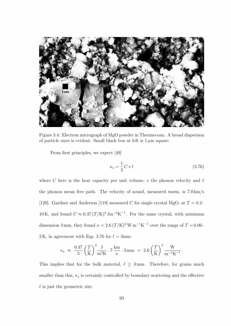
Figure 3.4: Electron micrograph of MgO powder in Thermocoax. A broad dispersionof particle sizes is evident. Small black box at left is 1µm square.
From first principles, we expect [49]
κs =1
3C v ℓ (3.76)
where C here is the heat capacity per unit volume, v the phonon velocity and ℓ
the phonon mean free path. The velocity of sound, measured warm, is 7.0 km/s
[120]. Gardner and Anderson [119] measured C for single crystal MgO, at T = 0.2–
10 K, and found C ≈ 0.37 (T/K)3 Jm−3K−1. For the same crystal, with minimum
dimension 3 mm, they found κ = 2.6 (T/K)3 W m−1K−1 over the range of T = 0.06–
2 K, in agreement with Eqs. 3.76 for ℓ = 3mm:
κs ≈ 0.37
3
(
T
K
)3J
m3K· 7 km
s· 3 mm = 2.6
(
T
K
)3W
m−1K−1.
This implies that for the bulk material, ℓ ≥ 3 mm. Therefore, for grains much
smaller than this, κs is certainly controlled by boundary scattering and the effective
ℓ is just the geometric size.
93
To estimate κp for the powdered MgO in Thermocoax at low temperature, I re-
place ℓ = 3 mm in the above calculation with ℓ = 1 µm, the apparent grain size, and
multiply by the volume fraction (0.6). The result is κp = 5×10⁻⁴ (T/K)3 W m−1K−1.
This would appear to set an upper bound on κp, but is perhaps not too far above the
true value, since an independent method of estimation (see Appendix, Sec. 3.5.5)
yields a somewhat greater value.
Applying this as an estimate for κd of the Thermocoax dielectric, we have
for the radial thermal conductance per unit length (Sec. 3.5.1), using Eq. 3.52 but
neglecting any contact resistance between the metal and dielectric,
kr =2πκd
ln(rd/rw)= 2π · 5×10−4
(
T
K
)3W
m·K · ln(
175µm
85µm
)
= 2.3×10⁻³
(
T
K
)3W
m·K
I have here ignored contact resistance because the thermal resistance of the
powdered MgO is so large and is primarily due to many contacts between grains
of the material. Also, unlike the case with PTFE, thermal contraction of MgO is
quite small, about 0.12% [121], less than half that of the stainless steel jacket [4].
Therefore the tightly-packed MgO should not loosen on cooling.
The thermalization length is then (Eq. 3.55)
ζ =
√
Kw
kr
=
√
5×10⁻¹⁰ (T/K) W m·K−1
2.3×10⁻³ (T/K)3 W m−1K−1= 0.5
(
T
K
)−1
mm .
The result is a reassuringly short thermalization length, although it is as long as
5 cm at 10 mK. Without having done this calculation, we would not have known it
was not much longer.
94
3.5.5 Appendix to Sec. 3.5.4: Another method of estimating κp for
MgO
I have not found thermal conductivity data for powdered MgO at low temper-
ature. High-temperature data (300–1300 K) [7], taken in the presence of air or inert
gases, show thermal conductivity for powdered MgO which is strongly dependent
on factors including volume fraction, particle size, gas pressure and composition,
and which is 1–2 orders of magnitude lower than that of the solid crystal. The ratio
κs/κp is also not independent of temperature; in fact κp tends to increase by factors
of 2–3 over this temperature range, while κs decreases by almost an order of magni-
tude. This suggests a large role for gas conduction and radiative coupling between
grains in the conditions under which these values were measured (high temperature
and gas pressure).
Shapiro et al. [6] measured the thermal conductivity of powder and bead beds
of five ceramic and glassy materials, with particle sizes ranging from 50 µm–3 mm,
at temperatures of ∼55 C, under 19 kPa of mechanical pressure, and gas pressures
of 10–107 Pa. Their data show that gas conduction plays a dominant role at any gas
pressure above ∼0.1 Pa [6]. They also estimated that radiation would contribute
negligbly at these (and lower) temperatures.
Their data reveal a curious phenomenon: for sufficiently low gas pressure, all
of the powder bed samples tested had κp ≈ 0.1–0.2 W m−1 K−1 despite κs for the
solid materials varying over an order of magnitude (0.74–8.4W m−1 K−1). These
results are displayed in Table 3.5.5, along with representative values for the Vickers
95
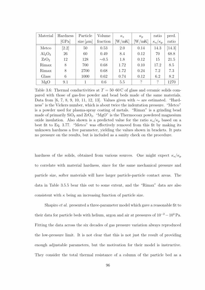
Material Hardness Particle Volume κs κp ratio pred.
[GPa] size [µm] fraction [W/m·K] [W/m·K] κs/κp ratio
Metco [2.2] 50 0.53 2.0 0.14 14.3 [14.3]
Al2O3 26 60 0.49 8.4 0.12 70 68.8
ZrO2 12 128 ∼0.5 1.8 0.12 15 21.5
Rimax 8 700 0.68 1.72 0.10 17.2 8.5
Rimax 8 2700 0.68 1.72 0.24 7.2 7.3
Glass 6 1000 0.62 0.74 0.12 6.2 8.2
MgO 9.1 1 0.6 5.5 ? ? 1270
Table 3.6: Thermal conductivities at T = 50–60 C of glass and ceramic solids com-pared with those of gas-free powder and bead beds made of the same materials.Data from [6, 7, 8, 9, 10, 11, 12, 13]. Values given with ∼ are estimated. “Hard-ness” is the Vickers number, which is about twice the indentation pressure. “Metco”is a powder used for plasma-spray coating of metals. “Rimax” is a grinding beadmade of primarily SiO2 and ZrO2. “MgO” is the Thermocoax powdered magnesiumoxide insulation. Also shown is a predicted value for the ratio κs/κp based on abest fit to Eq. 3.77. “Metco” was effectively removed from this fit by making itsunknown hardness a free parameter, yielding the values shown in brackets. It putsno pressure on the results, but is included as a sanity check on the procedure.
hardness of the solids, obtained from various sources. One might expect κs/κp
to correlate with material hardness, since for the same mechanical pressure and
particle size, softer materials will have larger particle-particle contact areas. The
data in Table 3.5.5 bear this out to some extent, and the “Rimax” data are also
consistent with κ being an increasing function of particle size.
Shapiro et al. presented a three-parameter model which gave a reasonable fit to
their data for particle beds with helium, argon and air at pressures of 10−2−104 Pa.
Fitting the data across the six decades of gas pressure variation always reproduced
the low-pressure limit. It is not clear that this is not just the result of providing
enough adjustable parameters, but the motivation for their model is instructive.
They consider the total thermal resistance of a column of the particle bed as a
96
sum of particle resistances and contact resistances, or equivalently total thermal
resistivity of the bed, considered as a bulk medium, as the sum of volume and
contact resistvity terms, ρv and ρc.
One may reasonably expect that, for a network of particles, and contacts
between them, that can be scaled by a single parameter d which we call the particle
size (which may be a peak in the distribution of linear dimensions of the particles),
ρv, the total thermal resistivity due to the bulk material, will be independent of d.
However, ρv may be expected to scale inversely to the average cross-sectional area,
or ρv ∝ f−2/3, where f is the volume packing fraction.
In addition, there will be a geometric factor due to heat flow through the
network being convoluted rather than simply parallel to the overall heat flow. This
factor is hard to estimate, but it will be of order unity, and will tend to increase
κs/κp. The geometric factor may reasonably be expected to be independent of the
particle size parameter.
Smaller particle size d will, on the other hand, mean proportionally more in-
terpositions of the contact resistance, hence one can write ρc ∝ d−1. Also, ρc should
be inversely proportional to the total area of each layer of contacts, or proportional
to hardness H divided by mechanical pressure pm, which is the inverse of the di-
mensionless fraction of cross-sectional area in contact per interfacial layer.
97
Summarizing, we can write
ρv = αv κ−1s f−2/3
ρc = αc κ−1s d−1H p−1
m
κp =1
ρv + ρc
=κs
αv
f 2/3+
αc
d
H
pm
, (3.77)
where the free parameters αv and αc incorporate the unknown shape factors and
relationship of interfacial resistances to solid resistivity.
Equation 3.77 can be considered a simplification of the Shapiro model in the
gas-free limit. It provides a basis for predicting κs/κp by comparison with other
materials. Shapiro et al. presented a somewhat more complicated form for the
dependence of ρc on contact area and hence on H and pm. However, the data shown
here does not provide an adequate basis for distinguishing which form provides a
better fit, so I use the simpler form.
By optimizing the parameters in Eq.3.77 to minimize squared residuals of
the predicted κs/κp for five of the Shapiro samples (Table 3.5.5), I calculated a
prediction of κs/κp = 1300 for 1µm MgO. Using κs = 2.6 (T/K)3 W m−1K−1, we find
κp = 2×10⁻³ (T/K)3 W m−1K−1.
The prediction for 1µm MgO is clearly an extrapolation outside the range (in
particle size) of the sample materials. It is encouraging that this result is within
an order of magnitude of that obtained by the method presented in the main text.
However, it is larger than that result. Since the method presented in the main text is
based on what seems a necessary assumption–that the mean free path for phonons is
limited by the grain size–I think the result by that method must be closer to reality.
98
3.5.6 Thermalization of unshielded wiring
The application of Eqs. 3.74 requires knowing the thermal conductances Kw
and kr. The former can be calculated for a wire directly from the thermal conduc-
tivity if it is known. The latter is the sum of boundary resistances as well as volume
thermal conductivity of the insulator.
To ensure low thermal conductance between refrigeration stages, very fine
resistive or superconducting wire is used. The need for a substantial number of
wires leads to the use of multiwire cables and looms. The use of twisted pair wiring
and the weave of wiring looms mean that each wire will be directly exposed to a
thermal anchoring surface only at a fraction of its length. Pressure cannot be applied
without risk of damaging the wire or insulation. Inevitably the use of some type of
potting material is the best one can do. This is generally a disordered polymer which
is expected to have thermal conductivity roughly ∝ T 2. The choice of a particular
material apparently makes little difference at mK temperatures [63, 122]. GE/IMI
7031 varnish is often used for convenience.
Thermalization of fine wires in cryogenic apparatus was modeled by Hust
[114], who calculated thermalization lengths based on mean thermal conductivities
of copper and constantan, bonded to a thermal anchor through a bridge of var-
nish. Hust’s calculations showed that for constantan wire of about 100µm diameter
bonded with 7031 varnish, only a few mm of contact are needed at 4 K. Similar re-
sults obtain for other resistive wires such as manganin, stainless steel and phosphor
bronze [4]. In the case of Cu, however, the required thermalization lengths, for the
99
same thickness of wire, are more than an order of magnitude greater. This follows
from the fact that for Cu with RRR of 50, at low temperature ρ ≈ 3×10⁻¹⁰Ωm,
whereas for constantan ρ ≈ 5×10⁻⁷Ωm. Applying Eqs. 3.3 and 3.55, we have
ζCu/ζconstantan =√
5×10⁻⁷/3×10−10 = 41.
Whereas at 4 K the thermalization lengths for varnish-bonded wire can be
estimated on the basis of the volume thermal conductivity of the varnish, at mK
temperatures the volume resistance increases as the square of temperature and is
overtaken by boundary resistance, which increases as T 3. For a 50µm radius wire
with a 13µm thick layer of insulation resting on a Cu surface and varnished to it, I
estimate, based on a rough numerical integration, that the varnish bridge plus the
insulation on the wire is equivalent to a 100µm wide strip of varnish that is 18µm
thick. The boundary resistance should be roughly equal to 1+2/π ≈ 1.6 times that
due to a 100µm wide strip of Cu–varnish boundary.
Available data for the thermal conductivity of GE/IMI 7031 varnish near and
below 1 K disagree by more than an order of magnitude (Tables 3.2. The lowest
value for the volume thermal conductivity was reported by Anderson and Peterson
[63], in a measurement which separated the volume term from the Kapitza term by
assuming that the volume conductivity was ∝ T 2 while the Kapitza resistance was
∝ T−3. These measurements were taken in the mK range (to 40 mK), and while it
is possible that they assigned too large a share of the total thermal resistance to the
volume component, the effective thickness I am assuming for the varnish film is only
a factor of 3 greater than the thickness in Anderson and Peterson’s study, which is
comparable and would only bias my use of their results in a conservative direction.
100
Therefore I use Anderson and Peterson’s data for both the volume and boundary
terms in preference to Stephens [64] who found much higher volume conductivity
(also in the mK range) but did not separate out the boundary term.
Thus, in the notation of Eq. 3.55, the thermal conductance kr from the wire
to the Cu anchor per unit length of the wire is found as:
kr = (RK + Rv)−1 =
[
1.6RK
10−4 m2/m+
(
κv100 µm
18 µm
)−1 ]−1
=
[
1.68.5×10−4(T/K)−3 m2K W−1
10−4 m+
(
3.5×10⁻³(T/K)2 W m−1K−1 100
18
)−1 ]−1
=
[
13.6
(
T
K
)−3
+ 51
(
T
K
)−2]−1W
m · K .
Note that while the boundary resistance term RK can safely be ignored at 4 K, it
is already significant at 1 K and becomes the dominant term below 0.3 K. Note also
that this result is based on the data of Anderson and Peterson, who reported a
relatively high value for the volume resistance. The calculations of Hust [114] and
values given by Ekin [4] for thermalization at 4.2 K ignore the boundary resistance.
The thermal conductance of the wire Kw, for 110µm constantan wire can be
calculated using the WFL law (Eq. 3.3) from the wire’s specified resistance Rw:
Kw = TL0
R= T
2.45×10⁻⁸ WΩK−2
66 Ω/m=
T
K· 3.7×10⁻¹⁰ W m
K.
For NbTi:CuNi wire with CuNi cross sectional area 3.1×10⁻⁹ m2, using the
data of Kushino [56] for 4.2–0.6 K, and of Greywall [54] for 100–10 mK (Table 3.1),
Kw is given by
Kw =
(
T
K
)1.1
2.5×10⁻¹⁰ W m
K, 4.2 − 0.6 K, and
Kw =T
K2.0×10−10 W m
K, 0.1 − 0.01 K.
101
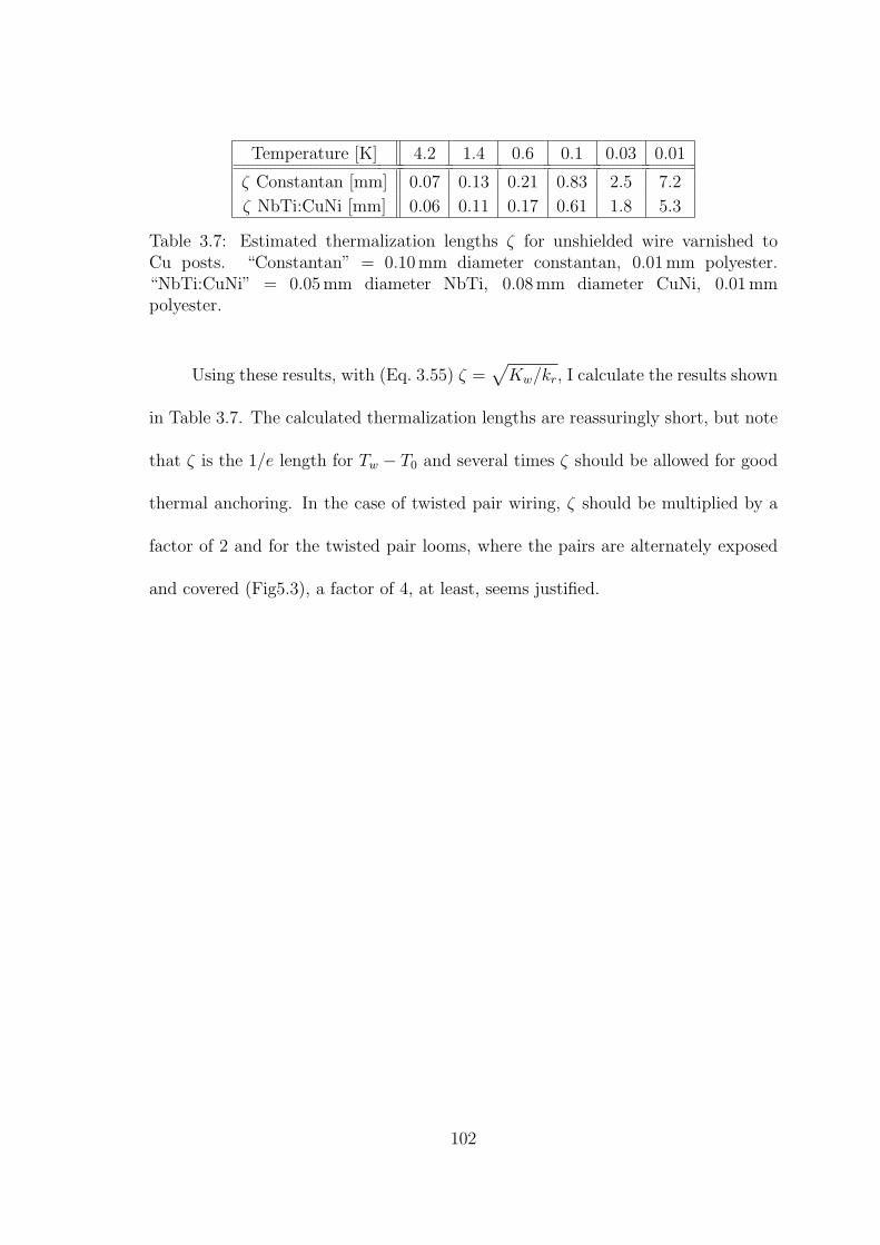
Temperature [K] 4.2 1.4 0.6 0.1 0.03 0.01
ζ Constantan [mm] 0.07 0.13 0.21 0.83 2.5 7.2
ζ NbTi:CuNi [mm] 0.06 0.11 0.17 0.61 1.8 5.3
Table 3.7: Estimated thermalization lengths ζ for unshielded wire varnished toCu posts. “Constantan” = 0.10 mm diameter constantan, 0.01 mm polyester.“NbTi:CuNi” = 0.05 mm diameter NbTi, 0.08 mm diameter CuNi, 0.01 mmpolyester.
Using these results, with (Eq. 3.55) ζ =√
Kw/kr, I calculate the results shown
in Table 3.7. The calculated thermalization lengths are reassuringly short, but note
that ζ is the 1/e length for Tw − T0 and several times ζ should be allowed for good
thermal anchoring. In the case of twisted pair wiring, ζ should be multiplied by a
factor of 2 and for the twisted pair looms, where the pairs are alternately exposed
and covered (Fig5.3), a factor of 4, at least, seems justified.
102
Chapter 4
Installation of cryostat, dilution refrigerator, pumps and plumbing
4.1 Basic facilities
A number of major design choices for the LPS mK-STM system were made
before I arrived at the lab in February 2006. The dilution refrigerator was chosen
to be an Oxford Kelvinox 400HA system [123] rated at 300µW cooling power at
100 mK, with a guaranteed base temperature <10 mK at installation, although the
operating temperature would certainly be somewhat higher. A superinsulated LHe
cryostat [124] was purchased from Kadel Engineering for initial use, and a second
cryostat with an integrated 13.5 T vertical solenoid magnet [125] was ordered from
American Magnetics for experiments requiring a high field.
The STM and UHV chamber system was designed by Barry Barker and
Michael Dreyer based on the 4 K STM system at LPS and similar systems built
at Berkeley, Hamburg and elsewhere [126]. The STM body is to be mounted below
the cold plate of the fridge, with a vertical transfer rod mechanism on the cryostat
central axis used to ferry samples and replacement tips up and down between the
STM body and a UHV chamber located directly above on top of the cryostat. A
second, horizontal transfer rod and associated piping allows transport of samples be-
tween the transfer chamber, a load lock chamber, and two auxiliary UHV chambers
for sample and tip preparation, characterization and storage.
103
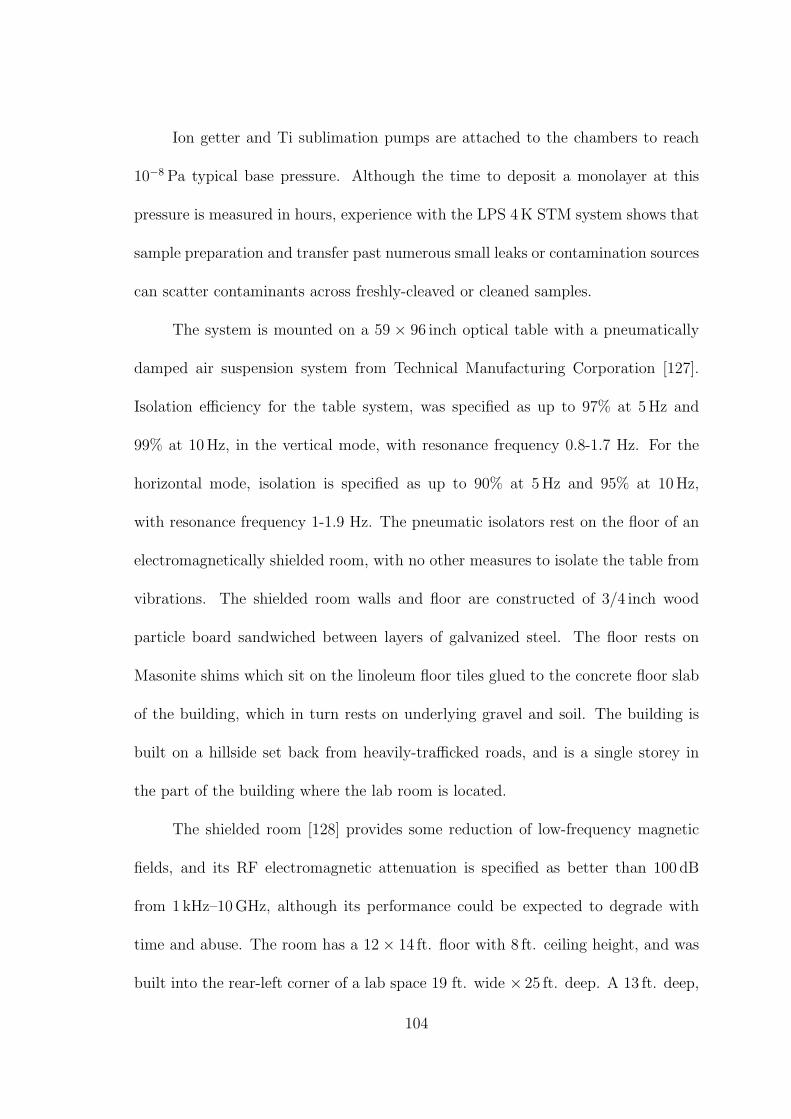
Ion getter and Ti sublimation pumps are attached to the chambers to reach
10−8 Pa typical base pressure. Although the time to deposit a monolayer at this
pressure is measured in hours, experience with the LPS 4 K STM system shows that
sample preparation and transfer past numerous small leaks or contamination sources
can scatter contaminants across freshly-cleaved or cleaned samples.
The system is mounted on a 59 × 96 inch optical table with a pneumatically
damped air suspension system from Technical Manufacturing Corporation [127].
Isolation efficiency for the table system, was specified as up to 97% at 5 Hz and
99% at 10 Hz, in the vertical mode, with resonance frequency 0.8-1.7 Hz. For the
horizontal mode, isolation is specified as up to 90% at 5 Hz and 95% at 10 Hz,
with resonance frequency 1-1.9 Hz. The pneumatic isolators rest on the floor of an
electromagnetically shielded room, with no other measures to isolate the table from
vibrations. The shielded room walls and floor are constructed of 3/4 inch wood
particle board sandwiched between layers of galvanized steel. The floor rests on
Masonite shims which sit on the linoleum floor tiles glued to the concrete floor slab
of the building, which in turn rests on underlying gravel and soil. The building is
built on a hillside set back from heavily-trafficked roads, and is a single storey in
the part of the building where the lab room is located.
The shielded room [128] provides some reduction of low-frequency magnetic
fields, and its RF electromagnetic attenuation is specified as better than 100 dB
from 1 kHz–10 GHz, although its performance could be expected to degrade with
time and abuse. The room has a 12 × 14 ft. floor with 8 ft. ceiling height, and was
built into the rear-left corner of a lab space 19 ft. wide × 25 ft. deep. A 13 ft. deep,
104
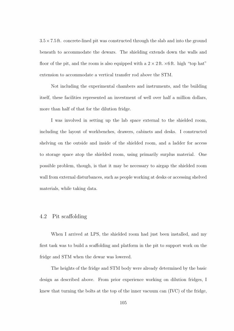
3.5×7.5 ft. concrete-lined pit was constructed through the slab and into the ground
beneath to accommodate the dewars. The shielding extends down the walls and
floor of the pit, and the room is also equipped with a 2× 2 ft.×6 ft. high “top hat”
extension to accommodate a vertical transfer rod above the STM.
Not including the experimental chambers and instruments, and the building
itself, these facilities represented an investment of well over half a million dollars,
more than half of that for the dilution fridge.
I was involved in setting up the lab space external to the shielded room,
including the layout of workbenches, drawers, cabinets and desks. I constructed
shelving on the outside and inside of the shielded room, and a ladder for access
to storage space atop the shielded room, using primarily surplus material. One
possible problem, though, is that it may be necessary to airgap the shielded room
wall from external disturbances, such as people working at desks or accessing shelved
materials, while taking data.
4.2 Pit scaffolding
When I arrived at LPS, the shielded room had just been installed, and my
first task was to build a scaffolding and platform in the pit to support work on the
fridge and STM when the dewar was lowered.
The heights of the fridge and STM body were already determined by the basic
design as described above. From prior experience working on dilution fridges, I
knew that turning the bolts at the top of the inner vacuum can (IVC) of the fridge,
105
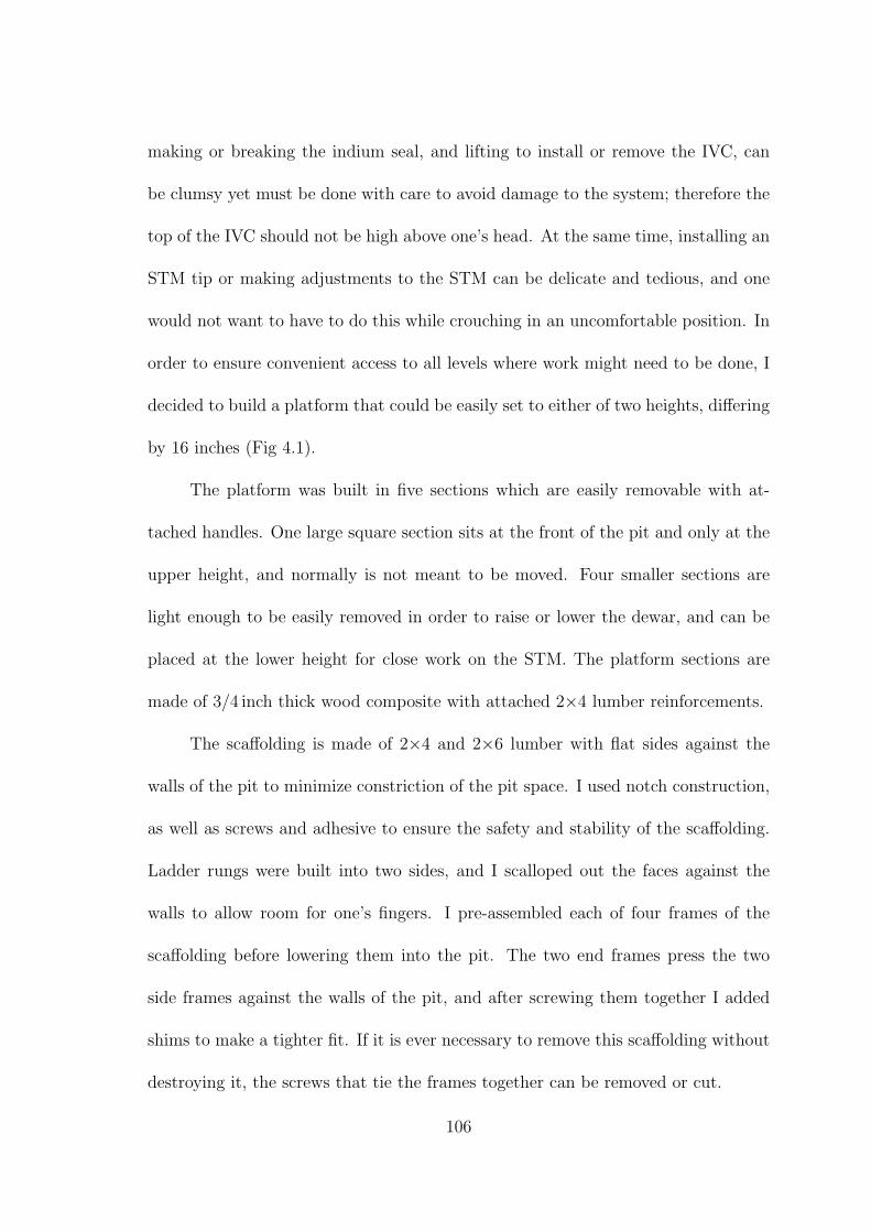
making or breaking the indium seal, and lifting to install or remove the IVC, can
be clumsy yet must be done with care to avoid damage to the system; therefore the
top of the IVC should not be high above one’s head. At the same time, installing an
STM tip or making adjustments to the STM can be delicate and tedious, and one
would not want to have to do this while crouching in an uncomfortable position. In
order to ensure convenient access to all levels where work might need to be done, I
decided to build a platform that could be easily set to either of two heights, differing
by 16 inches (Fig 4.1).
The platform was built in five sections which are easily removable with at-
tached handles. One large square section sits at the front of the pit and only at the
upper height, and normally is not meant to be moved. Four smaller sections are
light enough to be easily removed in order to raise or lower the dewar, and can be
placed at the lower height for close work on the STM. The platform sections are
made of 3/4 inch thick wood composite with attached 2×4 lumber reinforcements.
The scaffolding is made of 2×4 and 2×6 lumber with flat sides against the
walls of the pit to minimize constriction of the pit space. I used notch construction,
as well as screws and adhesive to ensure the safety and stability of the scaffolding.
Ladder rungs were built into two sides, and I scalloped out the faces against the
walls to allow room for one’s fingers. I pre-assembled each of four frames of the
scaffolding before lowering them into the pit. The two end frames press the two
side frames against the walls of the pit, and after screwing them together I added
shims to make a tighter fit. If it is ever necessary to remove this scaffolding without
destroying it, the screws that tie the frames together can be removed or cut.
106
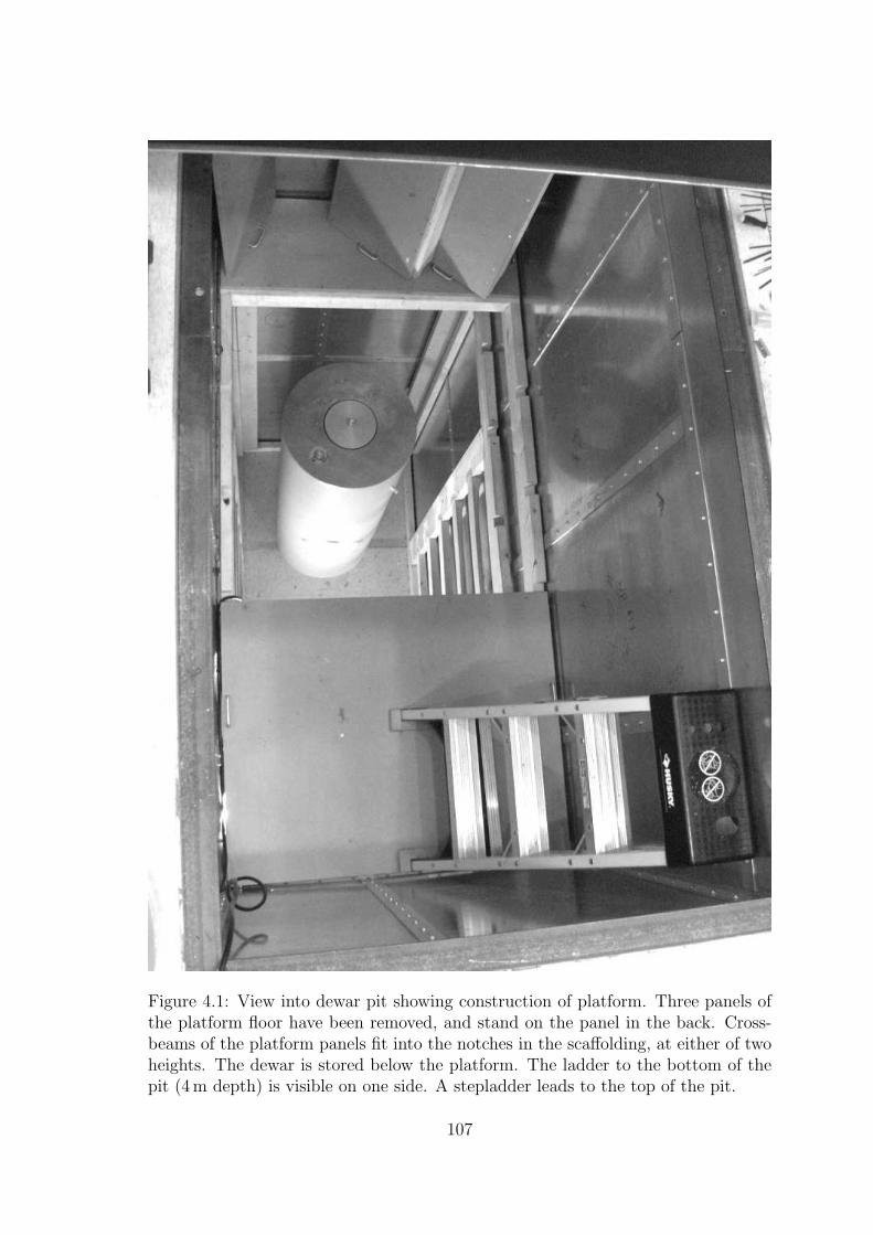
Figure 4.1: View into dewar pit showing construction of platform. Three panels ofthe platform floor have been removed, and stand on the panel in the back. Cross-beams of the platform panels fit into the notches in the scaffolding, at either of twoheights. The dewar is stored below the platform. The ladder to the bottom of thepit (4 m depth) is visible on one side. A stepladder leads to the top of the pit.
107
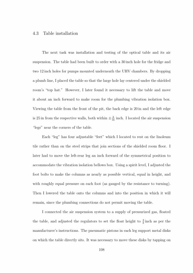
4.3 Table installation
The next task was installation and testing of the optical table and its air
suspension. The table had been built to order with a 30 inch hole for the fridge and
two 12 inch holes for pumps mounted underneath the UHV chambers. By dropping
a plumb line, I placed the table so that the large hole lay centered under the shielded
room’s “top hat.” However, I later found it necessary to lift the table and move
it about an inch forward to make room for the plumbing vibration isolation box.
Viewing the table from the front of the pit, the back edge is 20 in and the left edge
is 25 in from the respective walls, both within ± 3
16inch. I located the air suspension
“legs” near the corners of the table.
Each “leg” has four adjustable “feet” which I located to rest on the linoleum
tile rather than on the steel strips that join sections of the shielded room floor. I
later had to move the left-rear leg an inch forward of the symmetrical position to
accommodate the vibration isolation bellows box. Using a spirit level, I adjusted the
foot bolts to make the columns as nearly as possible vertical, equal in height, and
with roughly equal pressure on each foot (as gauged by the resistance to turning).
Then I lowered the table onto the columns and into the position in which it will
remain, since the plumbing connections do not permit moving the table.
I connected the air suspension system to a supply of pressurized gas, floated
the table, and adjusted the regulators to set the float height to 3
8inch as per the
manufacturer’s instructions. The pneumatic pistons in each leg support metal disks
on which the table directly sits. It was necessary to move these disks by tapping on
108
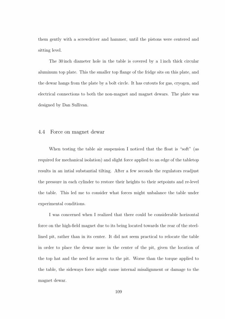
them gently with a screwdriver and hammer, until the pistons were centered and
sitting level.
The 30 inch diameter hole in the table is covered by a 1 inch thick circular
aluminum top plate. This the smaller top flange of the fridge sits on this plate, and
the dewar hangs from the plate by a bolt circle. It has cutouts for gas, cryogen, and
electrical connections to both the non-magnet and magnet dewars. The plate was
designed by Dan Sullivan.
4.4 Force on magnet dewar
When testing the table air suspension I noticed that the float is “soft” (as
required for mechanical isolation) and slight force applied to an edge of the tabletop
results in an intial substantial tilting. After a few seconds the regulators readjust
the pressure in each cylinder to restore their heights to their setpoints and re-level
the table. This led me to consider what forces might unbalance the table under
experimental conditions.
I was concerned when I realized that there could be considerable horizontal
force on the high-field magnet due to its being located towards the rear of the steel-
lined pit, rather than in its center. It did not seem practical to relocate the table
in order to place the dewar more in the center of the pit, given the location of
the top hat and the need for access to the pit. Worse than the torque applied to
the table, the sideways force might cause internal misalignment or damage to the
magnet dewar.
109
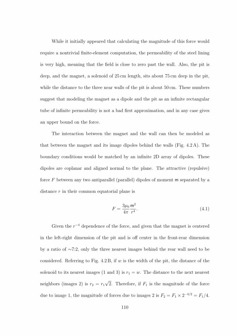
While it initially appeared that calculating the magnitude of this force would
require a nontrivial finite-element computation, the permeability of the steel lining
is very high, meaning that the field is close to zero past the wall. Also, the pit is
deep, and the magnet, a solenoid of 25 cm length, sits about 75 cm deep in the pit,
while the distance to the three near walls of the pit is about 50 cm. These numbers
suggest that modeling the magnet as a dipole and the pit as an infinite rectangular
tube of infinite permeability is not a bad first approximation, and in any case gives
an upper bound on the force.
The interaction between the magnet and the wall can then be modeled as
that between the magnet and its image dipoles behind the walls (Fig. 4.2 A). The
boundary conditions would be matched by an infinite 2D array of dipoles. These
dipoles are coplanar and aligned normal to the plane. The attractive (repulsive)
force F between any two antiparallel (parallel) dipoles of moment m separated by a
distance r in their common equatorial plane is
F =3µ0
4π
m2
r4. (4.1)
Given the r−4 dependence of the force, and given that the magnet is centered
in the left-right dimension of the pit and is off center in the front-rear dimension
by a ratio of ∼7:2, only the three nearest images behind the rear wall need to be
considered. Referring to Fig. 4.2 B, if w is the width of the pit, the distance of the
solenoid to its nearest images (1 and 3) is r1 = w. The distance to the next nearest
neighbors (images 2) is r2 = r1
√2. Therefore, if F1 is the magnitude of the force
due to image 1, the magnitude of forces due to images 2 is F2 = F1 × 2−4/2 = F1/4.
110
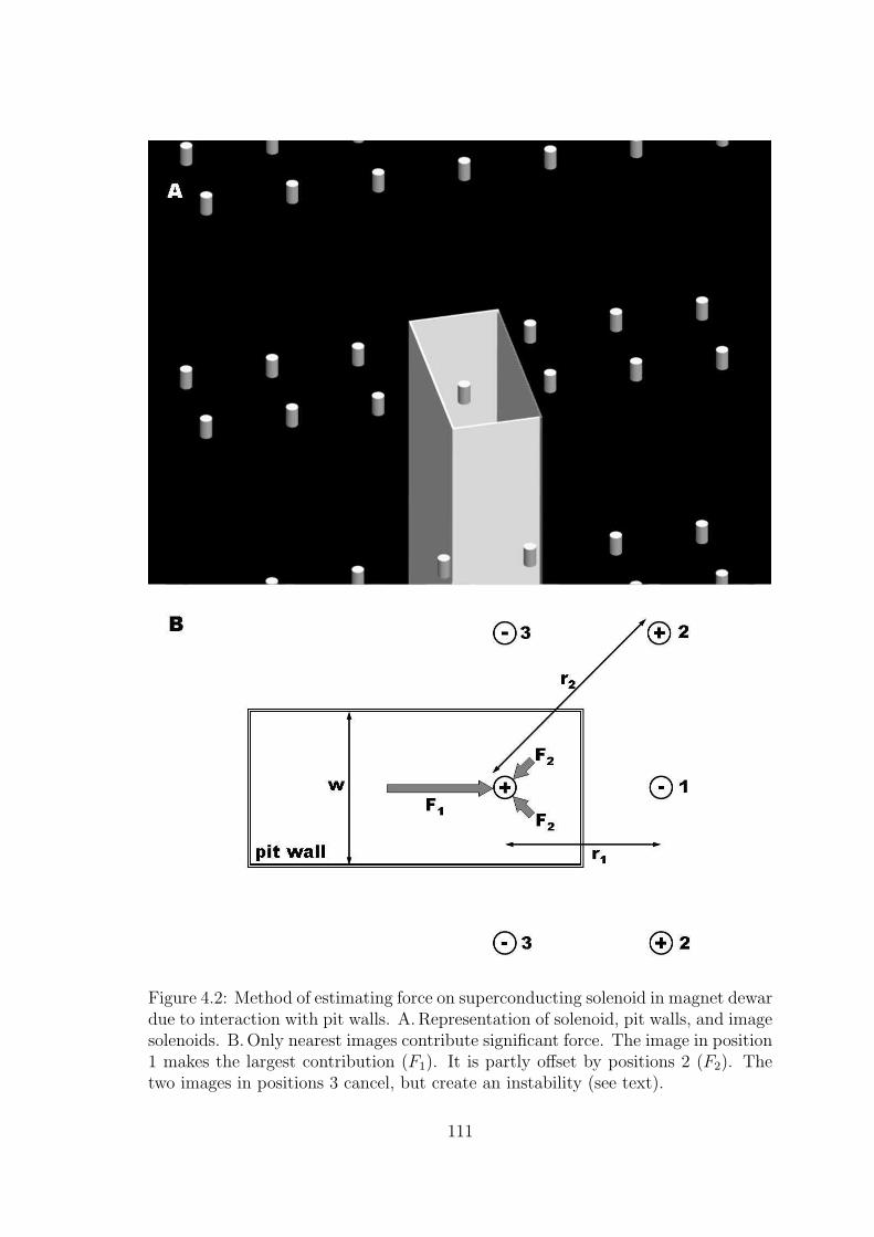
Figure 4.2: Method of estimating force on superconducting solenoid in magnet dewardue to interaction with pit walls. A. Representation of solenoid, pit walls, and imagesolenoids. B. Only nearest images contribute significant force. The image in position1 makes the largest contribution (F1). It is partly offset by positions 2 (F2). Thetwo images in positions 3 cancel, but create an instability (see text).
111
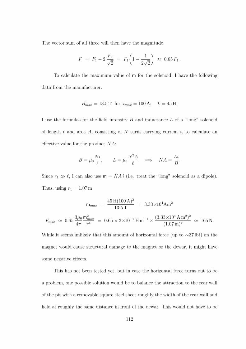
The vector sum of all three will then have the magnitude
F = F1 − 2F2√
2= F1
(
1 − 1
2√
2
)
≈ 0.65 F1 .
To calculate the maximum value of m for the solenoid, I have the following
data from the manufacturer:
Bmax = 13.5 T for imax = 100 A; L = 45 H.
I use the formulas for the field intensity B and inductance L of a “long” solenoid
of length ℓ and area A, consisting of N turns carrying current i, to calculate an
effective value for the product NA:
B = µ0
Ni
ℓ, L = µ0
N2A
ℓ=⇒ NA =
Li
B.
Since r1 ≫ ℓ, I can also use m = NA i (i.e. treat the “long” solenoid as a dipole).
Thus, using r1 = 1.07 m
mmax =45 H(100 A)2
13.5 T= 3.33×10⁴Am2
Fmax ≃ 0.653µ0
4π
m2max
r4= 0.65 × 3×10−7 H m−1 × (3.33×104 A m2)2
(1.07 m)4≃ 165 N.
While it seems unlikely that this amount of horizontal force (up to ∼37 lbf) on the
magnet would cause structural damage to the magnet or the dewar, it might have
some negative effects.
This has not been tested yet, but in case the horizontal force turns out to be
a problem, one possible solution would be to balance the attraction to the rear wall
of the pit with a removable square steel sheet roughly the width of the rear wall and
held at roughly the same distance in front of the dewar. This would not have to be
112
as heavy as it sounds, since the sheet could be thin and supported by a lightweight
frame. The balance could be fine-tuned by mounting a laser or stick pointer to reveal
any deflection of the floating table, and ramping the magnet current to detect an
unbalanced condition by observing the deflection. Once the correct distance for the
removable sheet is found, brackets to hold it can be fixed in position, and further
adjustment should not be necessary.
Unfortunately, such a balance will be unstable, since the residual horizontal
force will be linear in small displacements of the magnet from the balanced position.
This is a potential issue not just for the proposed front-rear balancing scheme, but
for the existing unstable right-left balance. Differentiating (4.1) gives:
∣
∣
∣
∣
dF
dr
∣
∣
∣
∣
=3µ0
π
m2
r5.
and the resultant sideways force in the direction of a small displacement left or right
from the center position (and front or back if the balancing scheme is used) will
be four times this since the two image dipoles will each move closer and further by
twice the displacement. Thus for the parameters here,
fmax
δ=
4Fmax
1.07 m= 4.8
N
cm,
where fmax is the force resulting in the direction of a small displacement δ for the
magnet at maximum current. This seems a large enough response (4.5 N≈ 1 lbf) to
worry about its potentially causing some instability.
Actually, if the center of mass of the entire system (table, fridge, dewar and
UHV chambers) lies above the plane of the air suspension pistons, the system is
already top-heavy and would be unstable if, for example, the air cylinders were
113
simply connected together, thus equalizing pressure in the cylinders, instead of using
the height regulators. With the regulators and internal damping, the air suspension
system is normally able to stabilize a top-heavy mass distribution, as when the table
is bare, or has heavy equipment mounted only on the top side.
An unstable balance of magnetic forces will add to any mechanical instability
resulting from a top-heavy system. The interaction of the magnetic field with the
steel may also be nonconservative, dissipating energy from the magnet. Combined
with the dynamic response of the table and its height regulators, one has to be
concerned about the possibility of oscillations under some conditions. Given the
complexity of the entire system, it may be easier to test whether this occurs than to
try to predict it. If problems do arise, it might be possible to stabilize the system
by adding weights to the dewar or to other structures pendant from the bottom of
the table.1
In any case, I would be especially careful when testing the magnet in place for
the first time, starting with low field and watching for any signs of instability as the
field is increased. This should include deliberately perturbing the system to gauge
its response, bearing in mind that the magnet stores up to 2.2 MJ at high field and
that if oscillations occur they might grow out of control before the field could be
ramped back down.
1Another possibility would be to add a magnetic pole piece centered below the dewar, to createa restoring force when the axis of the magnet was off-center. However, for such a geometry therestoring force would be quadratic in small displacements, whereas the destabilizing force is linear.
114
4.5 Raising and lowering the dewar
My next task was to design and build a system for raising and lowering the
dewar between its storage position at the bottom of the pit, and its operating
position pendant from the table. For this purpose, the dewar is suspended from
its two lifting eyes via cables. The cables hang over two idler pulleys mounted on
the top plate. Therefore the dewar can be raised vertically by pulling the cables
horizontally, using a winch.
Based on my previous experience with a large dilution refrigerator, I felt it
would be worthwhile to use a variable-speed electric winch rather than a hand-
cranked one. The Golo winch [129] operates very smoothly, and with the use of a
variac can be made to go at very low speed when the dewar is passing delicate parts
of the fridge, or quite fast for covering the distance up and down into the pit. A
single operator can raise or lower the dewar by remote-controlling the winch, but
must pay close attention and must guide the dewar by hand to avoid collisions with
the helium siphon, cold trap, level meter, and baffles. Such “hangups” can cause
severe damage to the fridge if not noticed in time.
It was important that the cables wind neatly in a single layer on the winch
drum, so that the dewar would remain level as it was lifted and not suddenly jump
or tilt, possibly damaging the fridge. After some experimentation, I settled on
the arrangement shown in Fig. 4.3. Each successive turn winds neatly next to the
previous one because it is pulled to the center by the small angle φ. The full depth
of the table is used to provide a long enough baseline that φ does not become large
115
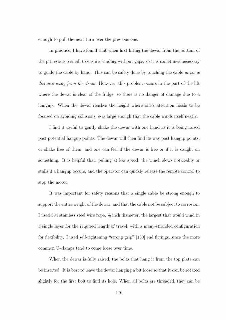
enough to pull the next turn over the previous one.
In practice, I have found that when first lifting the dewar from the bottom of
the pit, φ is too small to ensure winding without gaps, so it is sometimes necessary
to guide the cable by hand. This can be safely done by touching the cable at some
distance away from the drum. However, this problem occurs in the part of the lift
where the dewar is clear of the fridge, so there is no danger of damage due to a
hangup. When the dewar reaches the height where one’s attention needs to be
focused on avoiding collisions, φ is large enough that the cable winds itself neatly.
I find it useful to gently shake the dewar with one hand as it is being raised
past potential hangup points. The dewar will then find its way past hangup points,
or shake free of them, and one can feel if the dewar is free or if it is caught on
something. It is helpful that, pulling at low speed, the winch slows noticeably or
stalls if a hangup occurs, and the operator can quickly release the remote control to
stop the motor.
It was important for safety reasons that a single cable be strong enough to
support the entire weight of the dewar, and that the cable not be subject to corrosion.
I used 304 stainless steel wire rope, 5
32inch diameter, the largest that would wind in
a single layer for the required length of travel, with a many-stranded configuration
for flexibility. I used self-tightening “strong grip” [130] end fittings, since the more
common U-clamps tend to come loose over time.
When the dewar is fully raised, the bolts that hang it from the top plate can
be inserted. It is best to leave the dewar hanging a bit loose so that it can be rotated
slightly for the first bolt to find its hole. When all bolts are threaded, they can be
116
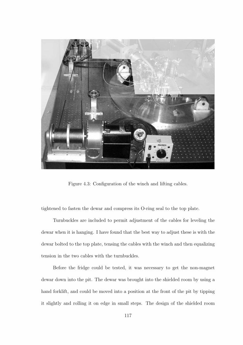
Figure 4.3: Configuration of the winch and lifting cables.
tightened to fasten the dewar and compress its O-ring seal to the top plate.
Turnbuckles are included to permit adjustment of the cables for leveling the
dewar when it is hanging. I have found that the best way to adjust these is with the
dewar bolted to the top plate, tensing the cables with the winch and then equalizing
tension in the two cables with the turnbuckles.
Before the fridge could be tested, it was necessary to get the non-magnet
dewar down into the pit. The dewar was brought into the shielded room by using a
hand forklift, and could be moved into a position at the front of the pit by tipping
it slightly and rolling it on edge in small steps. The design of the shielded room
117
included a steel I-beam over the pit to support lifting, but unfortunately this was
not centered over the part of the pit that is not covered by the table. I thought,
however, that lifting could be done at an angle if combined with a few strong men
pushing the dewar sideways. This method worked, but I would not recommend it. A
better method would be to use a bridge-type crane, at least one of which is available
at the LPS.
4.6 Initial testing of dilution refrigerator
Once the table was set up, it was possible to install the dilution fridge on the
table, set up pumps and plumbing lines temporarily and do an initial cooldown run.
This was done with the help of Mark Jackson of Oxford Instruments.
Examining a drawing of our non-magnet dewar, Mr. Jackson noticed a prob-
lem: it appeared the internal filling tube would interfere with the IVC of the fridge.
We could not reach deep into the dewar to bend the tube, and if we had been able
to, the tube would not have been long enough to reach the bottom of the dewar.
However, I was able to propose a repair: we could reach the tube near the top,
where it comes out into the wide belly of the dewar’s liquid helium space. We cut it
off there, leaving a stub of an inch or so, bent the tube into the desired shape, and
reinstalled it using a section of black Neoprene rubber hose to join the tube where
it was cut and to make up the lost length. The hose needed to be tightly clamped
since rubber expands on cooling. The repair remains in place to this day.
The pumps for the fridge were set up in the main lab room outside the shielded
118
room. The electrical supply and relay box for the pump system were installed in the
pump room. In order to connect the pumps and the system control panel to the relay
box, we broke a small hole in the wall with a sledgehammer, through which the cables
could pass. Plumbing connections to the fridge were made through a removable
access panel in the shielded room wall, and flexible stainless steel bellows were used
for the plumbing lines, including a fairly monstrous 10 ft. long, 4 inch diameter
bellows for the still pumping line. Initial cooldown and checkout procedures were
conducted by Mr. Jackson, and after cooldown, nuclear orientation thermometry
(NOT) was used to verify a base temperature of 6-7 mK. The cooling power was
also tested by applying 400µW of heat to the mixing chamber, with 40 mW of heat
to the still, and measuring the mixing chamber temperature as 101.8 mK with the
RuO2 resistance thermometer supplied with the fridge.
4.7 The Vibration Problem
Following initial testing of the fridge, I undertook the permanent reinstallation
of the pumps and plumbing lines. The problem was to identify and incorporate the
best feasible measures of isolation to prevent vibrations from the pumps and other
sources from being transmitted to the tabletop through the plumbing. A balance
needed to be struck between the effectiveness of various proposed measures and
the time and expense of developing and installing them. Although in principle
a straightforward engineering problem, given the resources and knowledge I had
available, this became largely a matter of intuition, aided by analysis of the physics
119
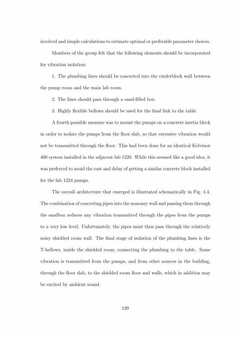
involved and simple calculations to estimate optimal or preferable parameter choices.
Members of the group felt that the following elements should be incorporated
for vibration isolation:
1. The plumbing lines should be concreted into the cinderblock wall between
the pump room and the main lab room.
2. The lines should pass through a sand-filled box.
3. Highly flexible bellows should be used for the final link to the table.
A fourth possible measure was to mount the pumps on a concrete inertia block
in order to isolate the pumps from the floor slab, so that excessive vibration would
not be transmitted through the floor. This had been done for an identical Kelvinox
400 system installed in the adjacent lab 1220. While this seemed like a good idea, it
was preferred to avoid the cost and delay of getting a similar concrete block installed
for the lab 1224 pumps.
The overall architecture that emerged is illustrated schematically in Fig. 4.4.
The combination of concreting pipes into the masonry wall and passing them through
the sandbox reduces any vibration transmitted through the pipes from the pumps
to a very low level. Unfortunately, the pipes must then pass through the relatively
noisy shielded room wall. The final stage of isolation of the plumbing lines is the
T-bellows, inside the shielded room, connecting the plumbing to the table. Some
vibration is transmitted from the pumps, and from other sources in the building,
through the floor slab, to the shielded room floor and walls, which in addition may
be excited by ambient sound.
120
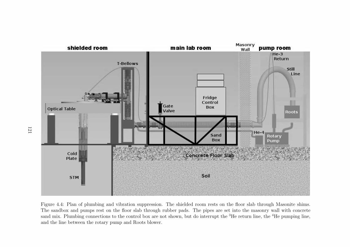
Figure 4.4: Plan of plumbing and vibration suppression. The shielded room rests on the floor slab through Masonite shims.The sandbox and pumps rest on the floor slab through rubber pads. The pipes are set into the masonry wall with concretesand mix. Plumbing connections to the control box are not shown, but do interrupt the 3He return line, the 4He pumping line,and the line between the rotary pump and Roots blower.
121
Figure 4.5 presents the vibration spectrum from 1-1200 Hz measured at the
tabletop on the top plate near the fridge/STM axis after reinstallation, with the
pumps running and the table floated; I introduce it here to show the range of
vibrations that are problematic and that needed to be minimized. These vibration
measurements were made with a velocity-sensitive geophone [131] consisting of a
fixed coil and moving spring-suspended permanent magnet which serves as the proof
mass. This sensor is usable at frequencies above ∼1 Hz and has a very flat frequency
response above ∼12 Hz, but I found that the coil picks up electromagnetic noise at
frequencies above ∼1.2 kHz.
Although the output voltage of the sensor is proportional to velocity, I have
chosen to display acceleration in Fig. 4.5 since, if, as expected, the resonant fre-
quency of the STM “figure G” is at least a few kHz, the tip-sample vibration am-
plitude in response to vibration below 1 kHz should be proportional to the force
experienced, i.e. acceleration. In fact, if the STM tip is modeled as a mass on a
spring, of resonant frequency fts, driven by motion of the tabletop at frequency f
with amplitude Atable, the resulting amplitude of tip sample motion Ats is given by
[132]
Trel ≡Ats
Atable
=F 2
√
(1 − F )2 + (2HF )2; (4.2)
where F ≡ ffts
and H ≡ ηηc
is the damping coefficient relative to critical damping.
Clearly, for F ≪ 1 and H < 1 we have Ats ≈ F 2Atable, i.e. tip-sample amplitude is
proportional to table acceleration.
The upper panel of Fig. 4.5 plots the rms acceleration per√
Hz on a logarithmic
122
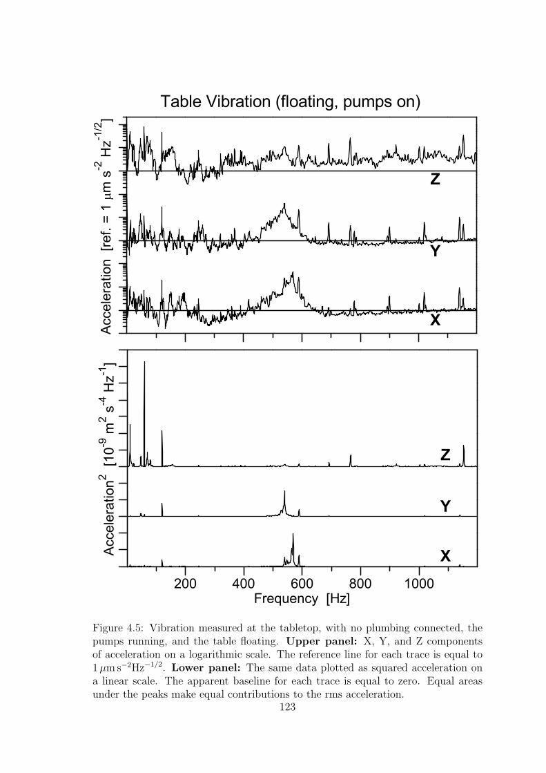
A
ccel
erat
ion
[ref
. = 1
m
s-2
Hz-1
/2]
Y
X
Z
Table Vibration (floating, pumps on)
200 400 600 800 1000
Acc
eler
atio
n2 [10
-9 m
2 s-4
Hz-1
]
Frequency [Hz]
Y
X
Z
Figure 4.5: Vibration measured at the tabletop, with no plumbing connected, thepumps running, and the table floating. Upper panel: X, Y, and Z componentsof acceleration on a logarithmic scale. The reference line for each trace is equal to1 µm s−2Hz−1/2. Lower panel: The same data plotted as squared acceleration ona linear scale. The apparent baseline for each trace is equal to zero. Equal areasunder the peaks make equal contributions to the rms acceleration.
123
scale, to show all portions of the spectrum. I checked the intrument noise floor with
an equivalent resistor and it was at well below the sensor output from 1-1200 Hz.
Note that the acceleration noise floor approaches 1µm/s2 Hz1/2 at the upper end of
the frequency range for the horizontal axes, and about a factor of 4 higher for Z. The
acceleration in the Z axis is generally higher, except for a hump around 500-600 Hz
in X and Y, which may represent a torsional resonance of the top plate with the
fridge and dewar bolted on.
However, since the response of the STM is expected to be flat in this low
frequency range, what matters is the square-integrated acceleration. The lower panel
of Fig. 4.5 shows the same spectrum plotted as (acceleration)2 per Hz; equal areas
under this curve make equal contributions to the square-integrated acceleration. It
is apparent that only a few frequency bands are significant. The peaks below 200
Hz correspond to noise from the pumps and other sources transmitted through the
floor and plumbing; higher frequencies are primarily transmitted to the table by
airborne sound.
4.8 Pump Room setup
4.8.1 Design
It was planned that the pumps would be installed in the adjacent pump room,
roughly 4 m from the nearest corner of the table. With a cinderblock wall interven-
ing, plus the shielded room wall, and with the possibility of adding sound-absorbing
materials as needed, we were not concerned with airborne sound from the pumps,
but only with low-frequency (< 200 Hz) vibration transmitted through the floor slab,
124
as well as any vibration transmitted through the plumbing lines.
There are three pumps: A small rotary vane pump for evacuating the 4He pot,
a larger rotary vane pump for circulating 3He, and a Roots blower for boosting 3He
circulation and lowering pressure in the still line. Each pump is a source of vibration.
However, although the Roots makes more audible noise, by far the strongest source
of low-frequency vibration that can be transmitted through the floor slab is the 3He
rotary circulation pump.
The data presented in Fig. 4.6 shows (top) the squared acceleration when the
pumps are on minus that when they are off, and (bottom) the squared acceleration
when only the main pump is on minus that when all pumps are off. The peaks
in these differences between 500-600 Hz for X and Y are attributable to changes in
the background sound exciting the “hump” that is observed at these frequencies
in Fig. 4.5, but are not consistent with attributing the “hump” to noise from the
pumps. Note that negative peaks in these traces would indicate that the table was
quieter with the pumps on, which only makes sense if the excitation comes from
other sources.
The difference peaks in Fig. 4.6 which are reproducible and attributable to
pump vibrations are at 59 Hz in Z only, and at 120 Hz in X, Y and Z. The largest
component of acceleration which can be attributed to the pumps is the one at 59 Hz.
It is about equally large in both the upper and lower panels, indicationg that it is
almost entirely accounted for by the 3He rotary pump alone. It appears that at least
some of the 120 Hz can be attributed to the other two pumps, or to other sources.
120 Hz vibration is common due to the interaction between magnetic fields from
125
60 Hz coils and nearby high-susceptibility parts, where frequency doubling results
from the fact that the force is attractive regardless of polarity.
The 3He rotary is a 2-vane pump (Fig. 4.10 A), with a nominal rotation speed
of 1640 rpm, or 27.3 Hz. It runs a little faster under high vacuum (if the motor
were under zero load, it would run at 30 Hz). However, the main component of the
vibration is at 59 Hz, double the rotation rate. This is probably due to the pair of
sliding vanes. Their center of mass lies on the pump axis when they are horizontal,
and below it when they are vertical, which occurs twice per cycle.
For each pump, the generation of oscillatory momentum, up to frequencies
comparable to any mechanical resonances of the pump case itself, can be modeled
as a periodic motion of some internal mass m relative to the mass M of the rigid case,
motor and remainder of the pump. In the simplest example, which approximates the
sliding vane pump, the motion can be described as an oscillation A cos(2πft) in the
vertical position of the center of m relative to M , along a line which passes through
the center of M . By momentum conservation, neglecting any forces transmitted
through the plumbing, wiring, or air, if the pump were floating in a zero gravity
environment, the case would simply vibrate with amplitude −A(m/M), so that the
center of mass of the entire pump remained stationary. However, if the case were
prevented from vibrating by being rigidly bolted to the floor, all of the oscillatory
momentum would necessarily be transmitted to the floor.
From the point of view of containing vibration, then, it would be best to
allow the pump to vibrate freely. This is approximately the situation if the pump
is supported by a sufficiently soft spring. However, the main pump weighs about
126
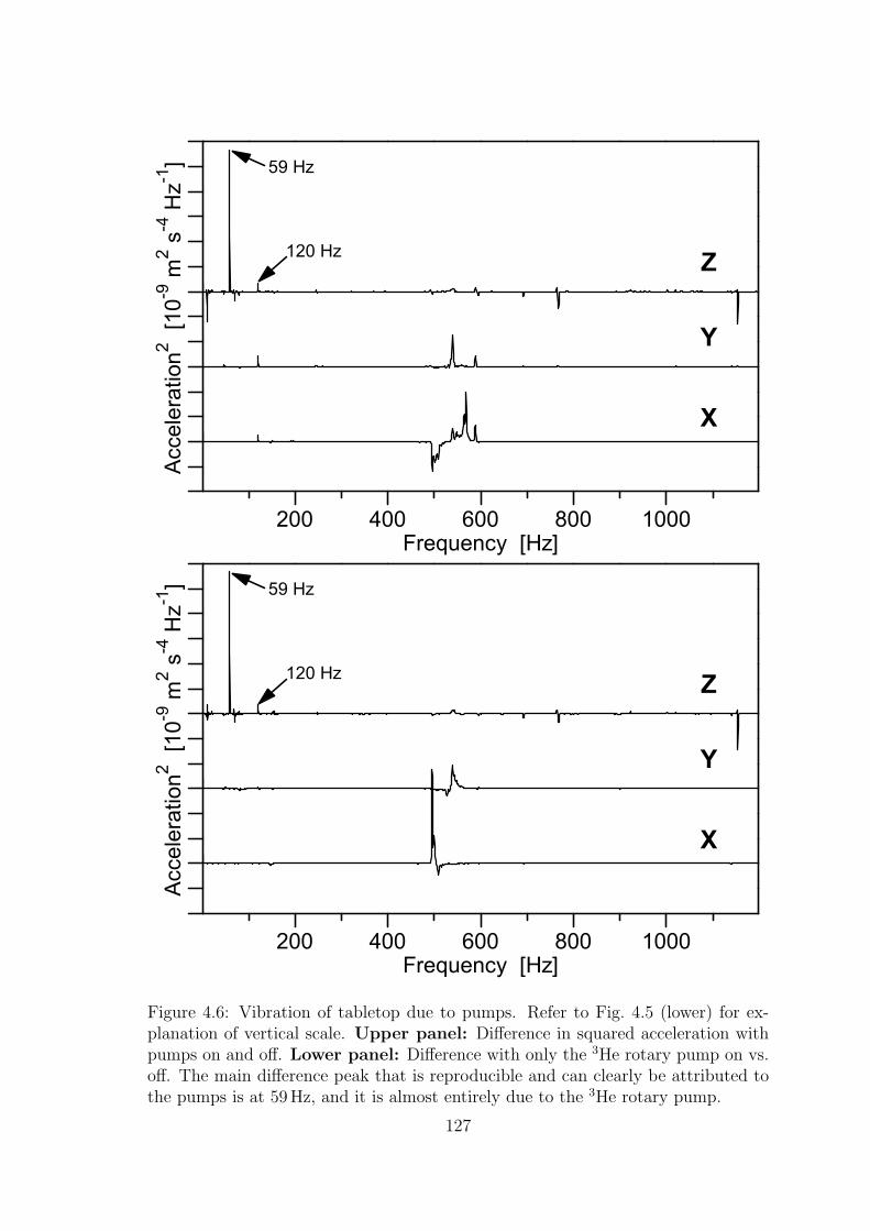
200 400 600 800 1000
Acc
eler
atio
n2 [10
-9 m
2 s-4
Hz-1
]
Frequency [Hz]
Y
X
Z
59 Hz
120 Hz
200 400 600 800 1000
Acc
eler
atio
n2 [10
-9 m
2 s-4
Hz-1
]
Frequency [Hz]
Y
X
Z
59 Hz
120 Hz
Figure 4.6: Vibration of tabletop due to pumps. Refer to Fig. 4.5 (lower) for ex-planation of vertical scale. Upper panel: Difference in squared acceleration withpumps on and off. Lower panel: Difference with only the 3He rotary pump on vs.off. The main difference peak that is reproducible and can clearly be attributed tothe pumps is at 59 Hz, and it is almost entirely due to the 3He rotary pump.
127
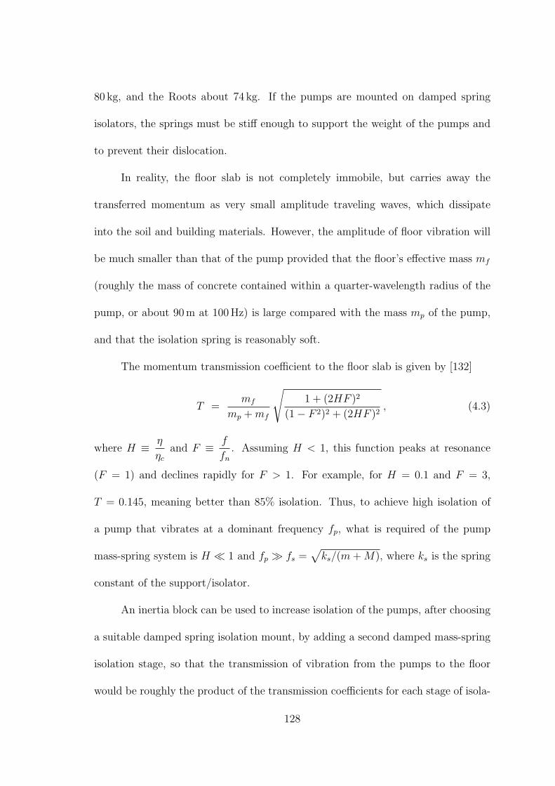
80 kg, and the Roots about 74 kg. If the pumps are mounted on damped spring
isolators, the springs must be stiff enough to support the weight of the pumps and
to prevent their dislocation.
In reality, the floor slab is not completely immobile, but carries away the
transferred momentum as very small amplitude traveling waves, which dissipate
into the soil and building materials. However, the amplitude of floor vibration will
be much smaller than that of the pump provided that the floor’s effective mass mf
(roughly the mass of concrete contained within a quarter-wavelength radius of the
pump, or about 90 m at 100 Hz) is large compared with the mass mp of the pump,
and that the isolation spring is reasonably soft.
The momentum transmission coefficient to the floor slab is given by [132]
T =mf
mp + mf
√
1 + (2HF )2
(1 − F 2)2 + (2HF )2, (4.3)
where H ≡ η
ηc
and F ≡ f
fn
. Assuming H < 1, this function peaks at resonance
(F = 1) and declines rapidly for F > 1. For example, for H = 0.1 and F = 3,
T = 0.145, meaning better than 85% isolation. Thus, to achieve high isolation of
a pump that vibrates at a dominant frequency fp, what is required of the pump
mass-spring system is H ≪ 1 and fp ≫ fs =√
ks/(m + M), where ks is the spring
constant of the support/isolator.
An inertia block can be used to increase isolation of the pumps, after choosing
a suitable damped spring isolation mount, by adding a second damped mass-spring
isolation stage, so that the transmission of vibration from the pumps to the floor
would be roughly the product of the transmission coefficients for each stage of isola-
128
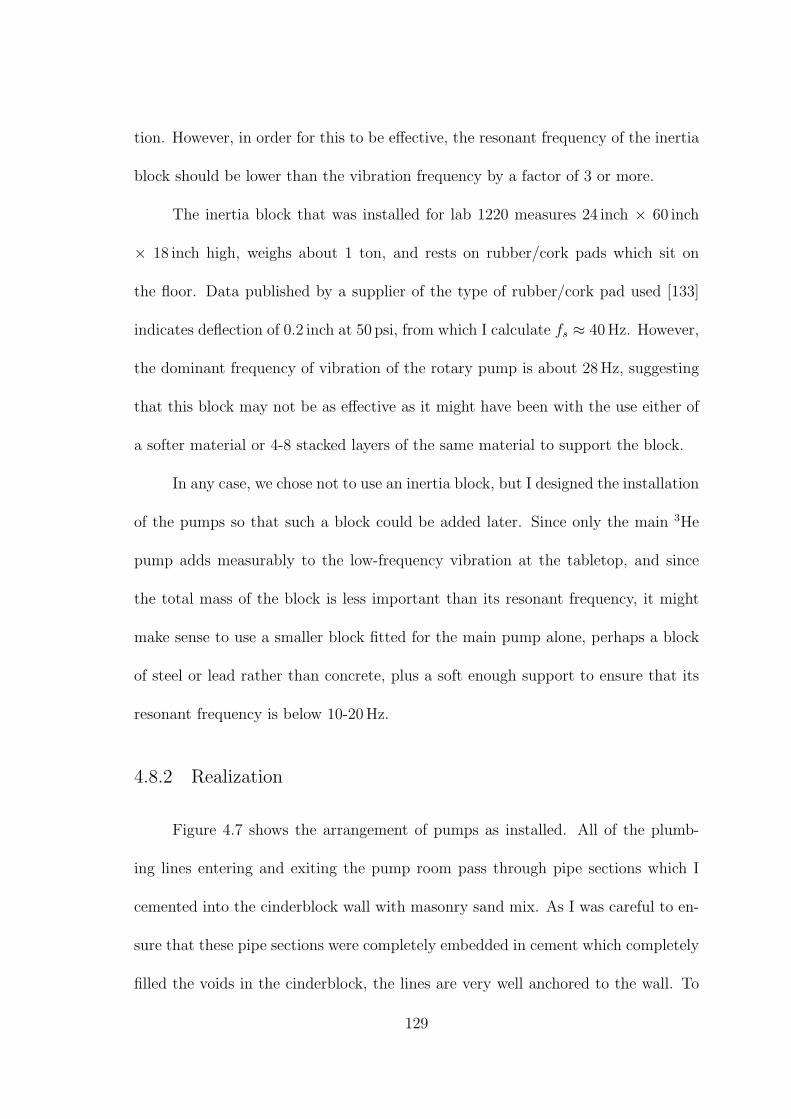
tion. However, in order for this to be effective, the resonant frequency of the inertia
block should be lower than the vibration frequency by a factor of 3 or more.
The inertia block that was installed for lab 1220 measures 24 inch × 60 inch
× 18 inch high, weighs about 1 ton, and rests on rubber/cork pads which sit on
the floor. Data published by a supplier of the type of rubber/cork pad used [133]
indicates deflection of 0.2 inch at 50 psi, from which I calculate fs ≈ 40 Hz. However,
the dominant frequency of vibration of the rotary pump is about 28 Hz, suggesting
that this block may not be as effective as it might have been with the use either of
a softer material or 4-8 stacked layers of the same material to support the block.
In any case, we chose not to use an inertia block, but I designed the installation
of the pumps so that such a block could be added later. Since only the main 3He
pump adds measurably to the low-frequency vibration at the tabletop, and since
the total mass of the block is less important than its resonant frequency, it might
make sense to use a smaller block fitted for the main pump alone, perhaps a block
of steel or lead rather than concrete, plus a soft enough support to ensure that its
resonant frequency is below 10-20 Hz.
4.8.2 Realization
Figure 4.7 shows the arrangement of pumps as installed. All of the plumb-
ing lines entering and exiting the pump room pass through pipe sections which I
cemented into the cinderblock wall with masonry sand mix. As I was careful to en-
sure that these pipe sections were completely embedded in cement which completely
filled the voids in the cinderblock, the lines are very well anchored to the wall. To
129
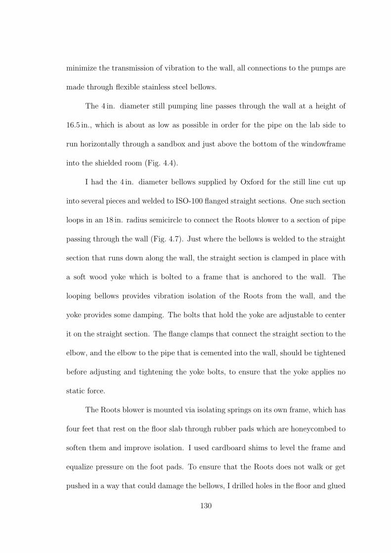
minimize the transmission of vibration to the wall, all connections to the pumps are
made through flexible stainless steel bellows.
The 4 in. diameter still pumping line passes through the wall at a height of
16.5 in., which is about as low as possible in order for the pipe on the lab side to
run horizontally through a sandbox and just above the bottom of the windowframe
into the shielded room (Fig. 4.4).
I had the 4 in. diameter bellows supplied by Oxford for the still line cut up
into several pieces and welded to ISO-100 flanged straight sections. One such section
loops in an 18 in. radius semicircle to connect the Roots blower to a section of pipe
passing through the wall (Fig. 4.7). Just where the bellows is welded to the straight
section that runs down along the wall, the straight section is clamped in place with
a soft wood yoke which is bolted to a frame that is anchored to the wall. The
looping bellows provides vibration isolation of the Roots from the wall, and the
yoke provides some damping. The bolts that hold the yoke are adjustable to center
it on the straight section. The flange clamps that connect the straight section to the
elbow, and the elbow to the pipe that is cemented into the wall, should be tightened
before adjusting and tightening the yoke bolts, to ensure that the yoke applies no
static force.
The Roots blower is mounted via isolating springs on its own frame, which has
four feet that rest on the floor slab through rubber pads which are honeycombed to
soften them and improve isolation. I used cardboard shims to level the frame and
equalize pressure on the foot pads. To ensure that the Roots does not walk or get
pushed in a way that could damage the bellows, I drilled holes in the floor and glued
130
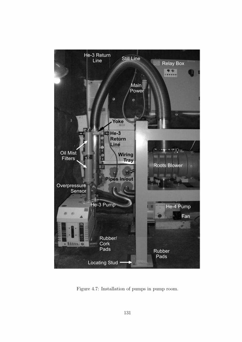
Figure 4.7: Installation of pumps in pump room.
131
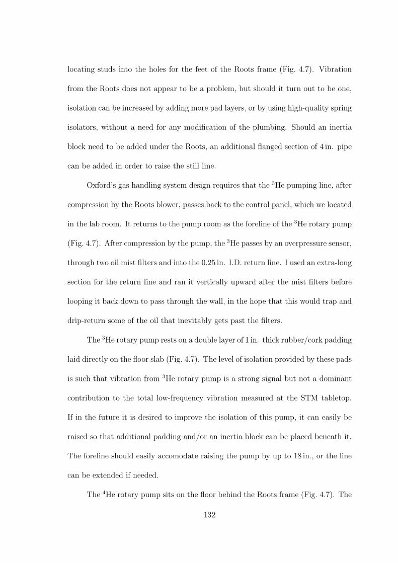
locating studs into the holes for the feet of the Roots frame (Fig. 4.7). Vibration
from the Roots does not appear to be a problem, but should it turn out to be one,
isolation can be increased by adding more pad layers, or by using high-quality spring
isolators, without a need for any modification of the plumbing. Should an inertia
block need to be added under the Roots, an additional flanged section of 4 in. pipe
can be added in order to raise the still line.
Oxford’s gas handling system design requires that the 3He pumping line, after
compression by the Roots blower, passes back to the control panel, which we located
in the lab room. It returns to the pump room as the foreline of the 3He rotary pump
(Fig. 4.7). After compression by the pump, the 3He passes by an overpressure sensor,
through two oil mist filters and into the 0.25 in. I.D. return line. I used an extra-long
section for the return line and ran it vertically upward after the mist filters before
looping it back down to pass through the wall, in the hope that this would trap and
drip-return some of the oil that inevitably gets past the filters.
The 3He rotary pump rests on a double layer of 1 in. thick rubber/cork padding
laid directly on the floor slab (Fig. 4.7). The level of isolation provided by these pads
is such that vibration from 3He rotary pump is a strong signal but not a dominant
contribution to the total low-frequency vibration measured at the STM tabletop.
If in the future it is desired to improve the isolation of this pump, it can easily be
raised so that additional padding and/or an inertia block can be placed beneath it.
The foreline should easily accomodate raising the pump by up to 18 in., or the line
can be extended if needed.
The 4He rotary pump sits on the floor behind the Roots frame (Fig. 4.7). The
132
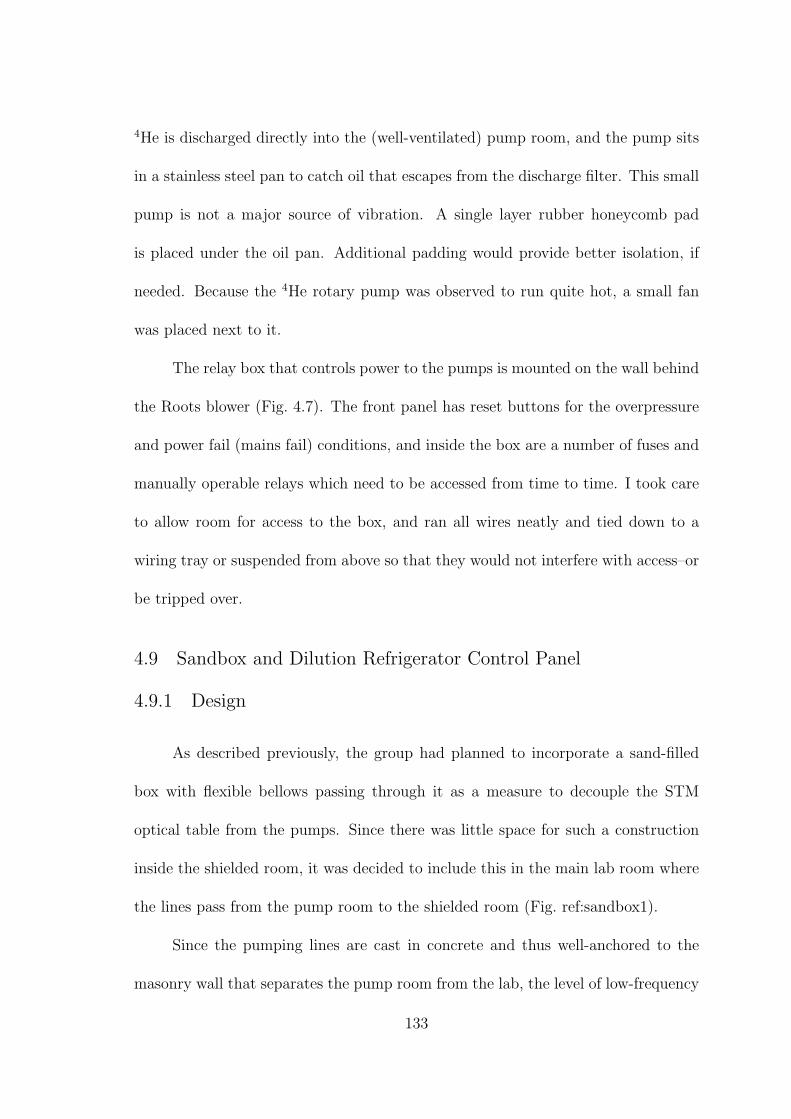
4He is discharged directly into the (well-ventilated) pump room, and the pump sits
in a stainless steel pan to catch oil that escapes from the discharge filter. This small
pump is not a major source of vibration. A single layer rubber honeycomb pad
is placed under the oil pan. Additional padding would provide better isolation, if
needed. Because the 4He rotary pump was observed to run quite hot, a small fan
was placed next to it.
The relay box that controls power to the pumps is mounted on the wall behind
the Roots blower (Fig. 4.7). The front panel has reset buttons for the overpressure
and power fail (mains fail) conditions, and inside the box are a number of fuses and
manually operable relays which need to be accessed from time to time. I took care
to allow room for access to the box, and ran all wires neatly and tied down to a
wiring tray or suspended from above so that they would not interfere with access–or
be tripped over.
4.9 Sandbox and Dilution Refrigerator Control Panel
4.9.1 Design
As described previously, the group had planned to incorporate a sand-filled
box with flexible bellows passing through it as a measure to decouple the STM
optical table from the pumps. Since there was little space for such a construction
inside the shielded room, it was decided to include this in the main lab room where
the lines pass from the pump room to the shielded room (Fig. ref:sandbox1).
Since the pumping lines are cast in concrete and thus well-anchored to the
masonry wall that separates the pump room from the lab, the level of low-frequency
133
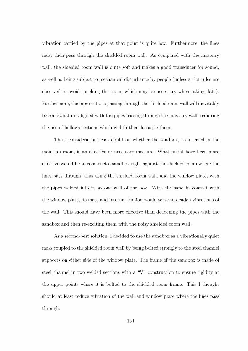
vibration carried by the pipes at that point is quite low. Furthermore, the lines
must then pass through the shielded room wall. As compared with the masonry
wall, the shielded room wall is quite soft and makes a good transducer for sound,
as well as being subject to mechanical disturbance by people (unless strict rules are
observed to avoid touching the room, which may be necessary when taking data).
Furthermore, the pipe sections passing through the shielded room wall will inevitably
be somewhat misaligned with the pipes passing through the masonry wall, requiring
the use of bellows sections which will further decouple them.
These considerations cast doubt on whether the sandbox, as inserted in the
main lab room, is an effective or necessary measure. What might have been more
effective would be to construct a sandbox right against the shielded room where the
lines pass through, thus using the shielded room wall, and the window plate, with
the pipes welded into it, as one wall of the box. With the sand in contact with
the window plate, its mass and internal friction would serve to deaden vibrations of
the wall. This should have been more effective than deadening the pipes with the
sandbox and then re-exciting them with the noisy shielded room wall.
As a second-best solution, I decided to use the sandbox as a vibrationally quiet
mass coupled to the shielded room wall by being bolted strongly to the steel channel
supports on either side of the window plate. The frame of the sandbox is made of
steel channel in two welded sections with a “V” construction to ensure rigidity at
the upper points where it is bolted to the shielded room frame. This I thought
should at least reduce vibration of the wall and window plate where the lines pass
through.
134
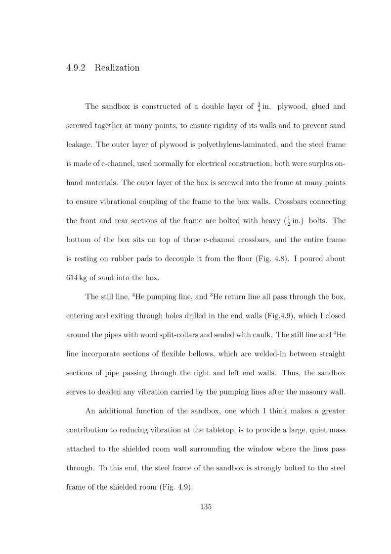
4.9.2 Realization
The sandbox is constructed of a double layer of 3
4in. plywood, glued and
screwed together at many points, to ensure rigidity of its walls and to prevent sand
leakage. The outer layer of plywood is polyethylene-laminated, and the steel frame
is made of c-channel, used normally for electrical construction; both were surplus on-
hand materials. The outer layer of the box is screwed into the frame at many points
to ensure vibrational coupling of the frame to the box walls. Crossbars connecting
the front and rear sections of the frame are bolted with heavy (1
2in.) bolts. The
bottom of the box sits on top of three c-channel crossbars, and the entire frame
is resting on rubber pads to decouple it from the floor (Fig. 4.8). I poured about
614 kg of sand into the box.
The still line, 4He pumping line, and 3He return line all pass through the box,
entering and exiting through holes drilled in the end walls (Fig.4.9), which I closed
around the pipes with wood split-collars and sealed with caulk. The still line and 4He
line incorporate sections of flexible bellows, which are welded-in between straight
sections of pipe passing through the right and left end walls. Thus, the sandbox
serves to deaden any vibration carried by the pumping lines after the masonry wall.
An additional function of the sandbox, one which I think makes a greater
contribution to reducing vibration at the tabletop, is to provide a large, quiet mass
attached to the shielded room wall surrounding the window where the lines pass
through. To this end, the steel frame of the sandbox is strongly bolted to the steel
frame of the shielded room (Fig. 4.9).
135
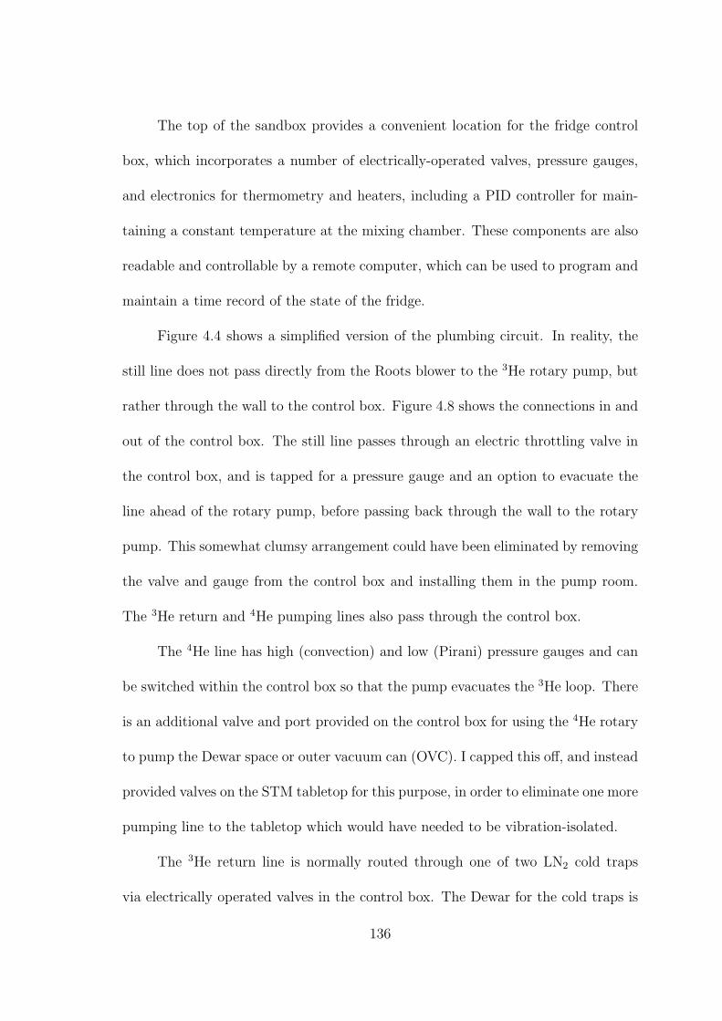
The top of the sandbox provides a convenient location for the fridge control
box, which incorporates a number of electrically-operated valves, pressure gauges,
and electronics for thermometry and heaters, including a PID controller for main-
taining a constant temperature at the mixing chamber. These components are also
readable and controllable by a remote computer, which can be used to program and
maintain a time record of the state of the fridge.
Figure 4.4 shows a simplified version of the plumbing circuit. In reality, the
still line does not pass directly from the Roots blower to the 3He rotary pump, but
rather through the wall to the control box. Figure 4.8 shows the connections in and
out of the control box. The still line passes through an electric throttling valve in
the control box, and is tapped for a pressure gauge and an option to evacuate the
line ahead of the rotary pump, before passing back through the wall to the rotary
pump. This somewhat clumsy arrangement could have been eliminated by removing
the valve and gauge from the control box and installing them in the pump room.
The 3He return and 4He pumping lines also pass through the control box.
The 4He line has high (convection) and low (Pirani) pressure gauges and can
be switched within the control box so that the pump evacuates the 3He loop. There
is an additional valve and port provided on the control box for using the 4He rotary
to pump the Dewar space or outer vacuum can (OVC). I capped this off, and instead
provided valves on the STM tabletop for this purpose, in order to eliminate one more
pumping line to the tabletop which would have needed to be vibration-isolated.
The 3He return line is normally routed through one of two LN2 cold traps
via electrically operated valves in the control box. The Dewar for the cold traps is
136
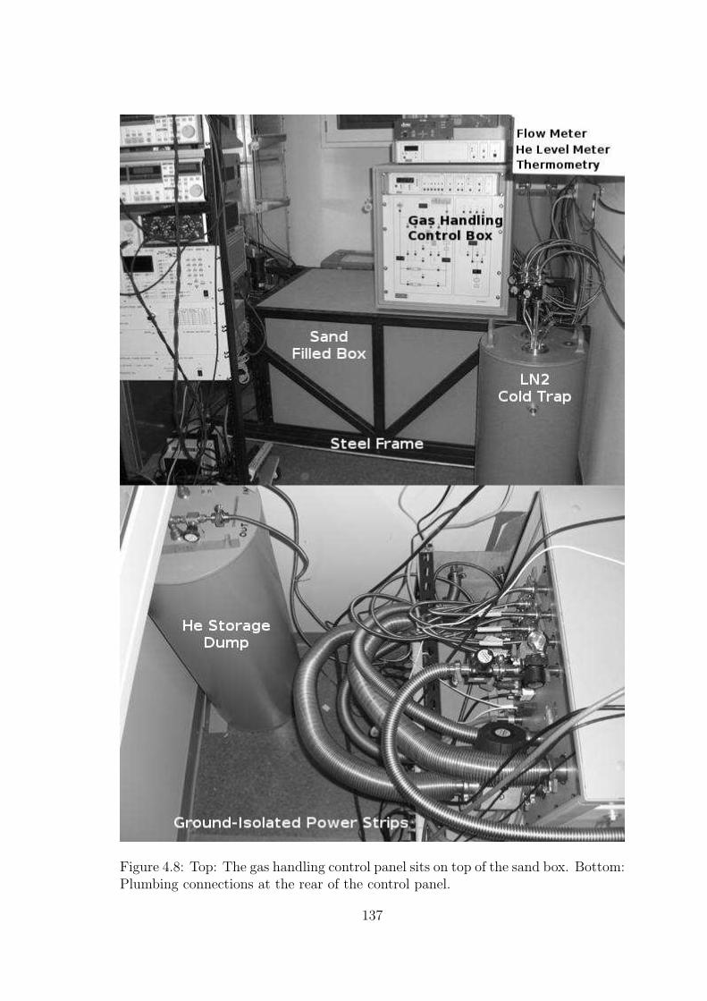
Figure 4.8: Top: The gas handling control panel sits on top of the sand box. Bottom:Plumbing connections at the rear of the control panel.
137
located directly in front of the control box (Fig. 4.8). When the fridge is warmed,
the 4He in the mixture comes out with the 3He and is stored in the dump, a 100 liter
tank located behind the sandbox. The dump also provides a place for the mixture to
go in case of blockage of the 3He line at any point after the rotary pump, or in case
the fridge warms up when unattended, e.g. after a power failure. The pressure relief
valves leading into the dump for this purpose begin to open at around 200 mbar
(which is a bit low). For this reason, the manual valve on the inlet side of the dump
(mounted atop the dump) must remain open at all times when operating the fridge.
I added manual valves directly on both sides of the cold traps for several
reasons. The electrically operated valves in the control box do not allow throttling to
control the flow rate. One of the valves is supposed to provide a variable impedance,
but in reality it gives very little control, going quickly from closed to wide open. In
addition, this valve leaks a bit when closed.
Another reason for the manual valves, and for having them on both the inlet
and outlet sides of each of the LN2 cold traps, is so that the traps can be detached
from the system, warmed to not greater than 100oC, and vacuum pumped in order
to remove water and other contaminants. Having valves attached directly to the
cold traps allows them to be kept under vacuum after cleaning. The lines can be
evacuated through the control box vent after reattaching them to the cold trap
valves (it is preferable not to pump the traps through the box while heating them).
Figure 4.9 shows the plumbing connections at each end of the sandbox. A
mass flow sensor is inserted in the 3He return line just before it enters the shielded
room. In operating the fridge, I have found it important to limit the flow below
138
Figure 4.9: Top: Connections from the pump room to the control box and sandbox. Bottom: Connections from the sand box into the shielded room.
139
200 sccm (standard cubic centimeter per minute) under all conditions. Higher flow
rates seem to lead to blockage of the LHe cold trap, probably by water or hydrogen
ice. Special care must be taken while condensing the mixture on cooldown, as the
flow rate into the fridge can initially be much higher. The flow rate can be limited
by throttling the manual valve coming out of the LN2 cold trap while watching the
flow rate meter.
A gate valve was also added to the still line just after it exits the shielded
room. Another manual valve was added to the still line where it enters the control
box after passing through the Roots blower. These valves are occasionally useful
for isolating the large volumes of the still line for leak checking or breaking vacuum.
They should otherwise be left open.
The window panel for the plumbing to the shielded room, actually a stainless
steel plate with pipes and fittings welded into it, also provides two spare vacuum
ports with NW-25 and NW-16 flanges, and two 1
4in. pressurized gas lines, one of
which is normally used to supply N2 into the room for levitating the table. An
electrical feedthru block provides 8 D-subminiature 15-pin connector feedthrus with
integral pi filters rated for 70 dB of attenuation at 1 GHz [134]. These lines are used
for fridge thermometry, heaters, the LHe level meter, and the electrically operated
needle valve for the 1 K pot, plus spare wires into the cryostat which can be used
for additional experimental or instrumentation purposes.
140
4.10 Vibration-Isolated Plumbing to Tabletop
4.10.1 Design
Plumbing connections to the tabletop present the most critical vibration iso-
lation problem, in order not to spoil the ability of the pneumatic supports to isolate
the table from the vibration of the shielded room floor. In fact, the vibration level
of the plumbing lines as they pass through the shielded room wall is higher than
that of the floor, even after the measures described above. Unfortunately, the wall
is not very stiff, and it makes a large diaphragm for transducing sound.
A vibration-isolated vacuum line is constructed out of flexible bellows, which
may be described as a pipe which is a soft rather than a very stiff spring. The 4 in.
diameter still line is particularly hard to isolate, since the spring constant of bellows
of any given type must scale as the square, at least, of its diameter. Two types of
bellows suitable for vacuum are available. Hydroformed bellows are essentially thin-
walled stainless steel tubing with circumferential ridges pressed in. Edge-welded
bellows are made of preformed concave washers welded together alternately at inner
and outer edges. The latter are more expensive but have lower spring constants,
and are needed to achieve good isolation.
The simplest way to use highly flexible edge-welded bellows would be to insert
a section of it into a line connecting to the table. By making this section sufficiently
long, the overall spring constant for static displacements could be made arbitrarily
low. However, the bellows has mass, hence for any given frequency its oscillatory
displacements will have a finite wavelength, and the length of the bellows that
141
is compressed by oscillatory force applied at one end will be limited to one-half
wavelength.
For example, I located a source [135] for stainless steel edge-welded bellows
having 102 mm (4 in.) ID, 145 mm OD, with longitudinal spring constant k speci-
fied as 2.45 N/mm for one segment, mass m = 0.225 kg per segment, and nominal
segment free length ℓ = 37.1 mm per segment. I calculate the longitudinal wave
velocity v as
v =
√
kℓ
m/ℓ= 0.0371 m ·
√
2450 kg m s−2/m
0.225 kg= 3.9
m
s(4.4)
which shows that for frequencies as low as 10 Hz, the effective spring constant cannot
be softened by increasing the length of this bellows beyond about 3.9 m/20 = 19 cm.
On the other hand, since the mass of the table is much greater than that of
the bellows, the induced motion of the table will be much smaller than the motion
of the bellows. High-frequency displacements will be reflected at each end, and the
bellows will have resonant modes for f = (n + 1
2)v
ℓ, where ℓ is now the total length
of the bellows.
The impulse delivered to the table will be proportional to the amplitude of
motion of the bellows. Therefore it is desirable that the half-wave resonant frequency
of the bellows (10 Hz for 19 cm in the case above) lie as low as possible below the
frequency range of concern. Damping will also affect the response of the bellows to
external vibration, particularly on resonance.
If the bellows is held vertically, and one end is subject to a small horizontal
displacement, the restoring force due to the bellows spring is quadratic, not linear,
142
in the horizontal displacement, since if the length of the bellows, when perfectly
vertical, is ℓ0, the extended length of the bellows when displaced horizontally by x
is ℓ =√
ℓ20 + x2, whence
dℓ
dx=
1
2
2x√
ℓ20 + x2
=⇒ dℓ
dx
∣
∣
∣
∣
x≪ℓ0
=x
ℓ0
. (4.5)
Thus if the spring constant of the bellows for extension of ℓ is k, the spring constant
for static horizontal displacement is kx
ℓ0
. For dynamic displacements at a given
frequency, ℓ0 will have some effective value less than the geometric length, but the
stiffness k will still be small for small amplitude displacements.
However, if the bellows is evacuated, extension of the bellows by dℓ will require
work dW = A dℓ × 1 atm., where A is the average cross-sectional area. If the
extension is due to a small static horizontal displacement dx, we can equate this to
the formula dW = kx dx for extension of a spring of constant k:
dW = A dℓ × 1 atm. =A
ℓ0
x dx × 1 atm. ≡ kx dx (4.6)
and thus find an effective spring constant k ≡ A
ℓ0
× 1 atm.
This effective spring constant for lateral displacement of an evacuated bellows
has been interpreted by some authors [136, 137] as “tension” in the bellows, but this
is a bit confusing since, if the bellows is held at both ends, the atmospheric pressure
on its cross-sectional area is borne by whatever is holding the ends. Pressure around
outer edges of each convolution of the bellows causes a local deformation equivalent
to compression, and the pressure around inner edges causes a local deformation
equivalent to extension, but the compression and extension alternate between inner
and outer edges. Thus there is no average deformation equivalent to an overall
143
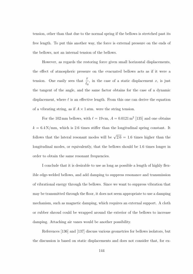
tension, other than that due to the normal spring if the bellows is stretched past its
free length. To put this another way, the force is external pressure on the ends of
the bellows, not an internal tension of the bellows.
However, as regards the restoring force given small horizontal displacements,
the effect of atmospheric pressure on the evacuated bellows acts as if it were a
tension. One easily sees thatx
ℓ0
, in the case of a static displacement x, is just
the tangent of the angle, and the same factor obtains for the case of a dynamic
displacement, where ℓ is an effective length. From this one can derive the equation
of a vibrating string, as if A × 1 atm. were the string tension.
For the 102 mm bellows, with ℓ = 19 cm, A = 0.0121 m2 [135] and one obtains
k = 6.4 N/mm, which is 2.6 times stiffer than the longitudinal spring constant. It
follows that the lateral resonant modes will be√
2.6 = 1.6 times higher than the
longitudinal modes, or equivalently, that the bellows should be 1.6 times longer in
order to obtain the same resonant frequencies.
I conclude that it is desirable to use as long as possible a length of highly flex-
ible edge-welded bellows, and add damping to suppress resonance and transmission
of vibrational energy through the bellows. Since we want to suppress vibration that
may be transmitted through the floor, it does not seem appropriate to use a damping
mechanism, such as magnetic damping, which requires an external support. A cloth
or rubber shroud could be wrapped around the exterior of the bellows to increase
damping. Attaching air vanes would be another possibility.
References [136] and [137] discuss various geometries for bellows isolators, but
the discussion is based on static displacements and does not consider that, for ex-
144
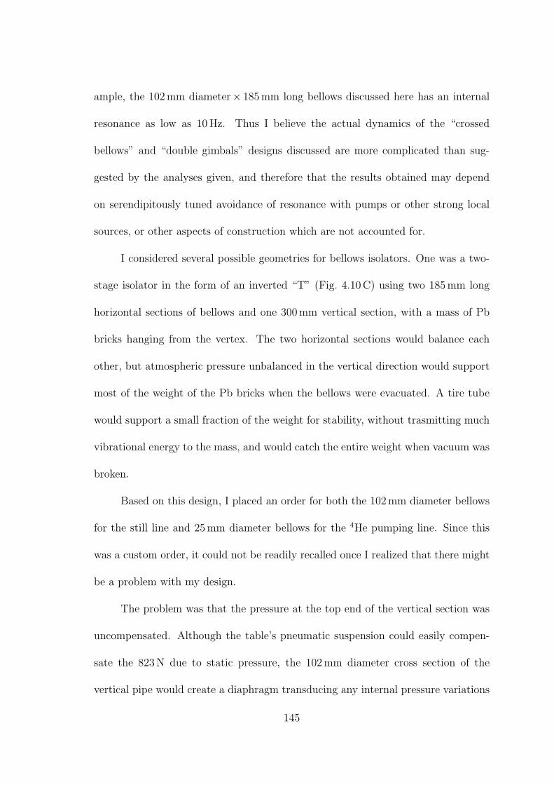
ample, the 102 mm diameter× 185 mm long bellows discussed here has an internal
resonance as low as 10 Hz. Thus I believe the actual dynamics of the “crossed
bellows” and “double gimbals” designs discussed are more complicated than sug-
gested by the analyses given, and therefore that the results obtained may depend
on serendipitously tuned avoidance of resonance with pumps or other strong local
sources, or other aspects of construction which are not accounted for.
I considered several possible geometries for bellows isolators. One was a two-
stage isolator in the form of an inverted “T” (Fig. 4.10 C) using two 185 mm long
horizontal sections of bellows and one 300 mm vertical section, with a mass of Pb
bricks hanging from the vertex. The two horizontal sections would balance each
other, but atmospheric pressure unbalanced in the vertical direction would support
most of the weight of the Pb bricks when the bellows were evacuated. A tire tube
would support a small fraction of the weight for stability, without trasmitting much
vibrational energy to the mass, and would catch the entire weight when vacuum was
broken.
Based on this design, I placed an order for both the 102 mm diameter bellows
for the still line and 25 mm diameter bellows for the 4He pumping line. Since this
was a custom order, it could not be readily recalled once I realized that there might
be a problem with my design.
The problem was that the pressure at the top end of the vertical section was
uncompensated. Although the table’s pneumatic suspension could easily compen-
sate the 823 N due to static pressure, the 102 mm diameter cross section of the
vertical pipe would create a diaphragm transducing any internal pressure variations
145
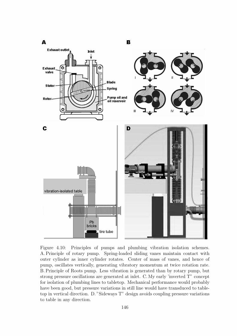
Figure 4.10: Principles of pumps and plumbing vibration isolation schemes.A. Principle of rotary pump. Spring-loaded sliding vanes maintain contact withouter cylinder as inner cylinder rotates. Center of mass of vanes, and hence ofpump, oscillates vertically, generating vibratory momentum at twice rotation rate.B. Principle of Roots pump. Less vibration is generated than by rotary pump, butstrong pressure oscillations are generated at inlet. C. My early ’inverted T” conceptfor isolation of plumbing lines to tabletop. Mechanical performance would probablyhave been good, but pressure variations in still line would have transduced to table-top in vertical direction. D. ”Sideways T” design avoids coupling pressure variationsto table in any direction.
146

to table vibration. Average pressure inside the still line at the table is expected to
be ∼30 Pa. The line is being pumped by the Roots blower (Fig. 4.10 B), which does
not operate like a continuous turbine but rather takes 240 scoops of gas per second.
The two lobes rotate at high speed and kick gas backward in part of each cycle as
well as drawing it forward. The 240 Hz pressure variation at the inlet of the Roots
is thus likely comparable to ±100% of the average pressure. While this pressure
variation is likely to be highly attenuated at the other end of the still line, the force
transmitted through the spring constant of the 102 mm bellows is ∼3×10⁻⁴ N for a
1 µm motion, whereas a 0.1 Pa pressure variation would transduce to 8×10⁻⁴ N force
on the table.
In order to avoid this potential problem, I decided to use a geometry (Fig. 4.10 D)
which would not transduce any pressure variation in the pumping lines to table mo-
tion. In this “sideways T” design, the vertex of the “T” is held by rigid pipe which
is clamped firmly to the table. Atmospheric pressure on the upper and lower ends of
the bellows is held by the frame and there is no net force on the table. I was able to
use the bellows as ordered, but the result is a bit strange-looking. In order to make
the bellows as long as possible, I used the longer sections for the lower bellows, and
clamped the two shorter sections together for the upper bellows.
4.10.2 Realization
I built the box to support the T-bellows (Figs. 4.11 and 4.12 using primarily
surplus material. The frame is made of Al channel and is strongly bolted together.
A heavy Al yoke holds the elbows at the lower ends, while the upper end of the still
147

line bellows is o-ring sealed directly to a plate that is bolted to the frame. Three
sides of the box are covered with Al-laminated Masonite panel, bolted at many
points to the frame, which provides both stiffening and damping. The open front
side is stiffened with diagonal crossbraces. By tapping on the box, one can tell that
it is quite vibrationally “dead.”
148
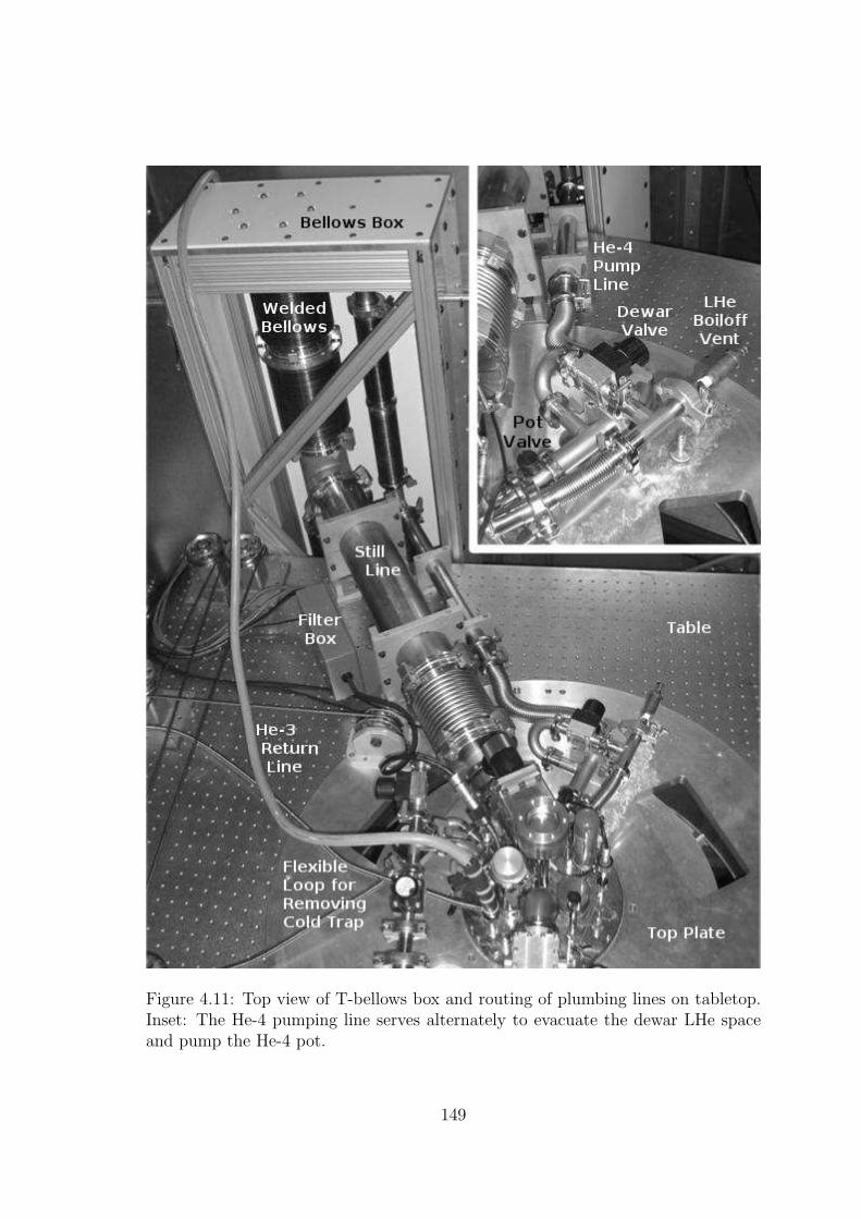
Figure 4.11: Top view of T-bellows box and routing of plumbing lines on tabletop.Inset: The He-4 pumping line serves alternately to evacuate the dewar LHe spaceand pump the He-4 pot.
149
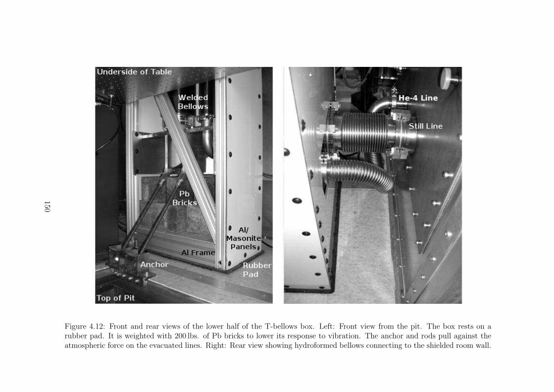
Figure 4.12: Front and rear views of the lower half of the T-bellows box. Left: Front view from the pit. The box rests on arubber pad. It is weighted with 200 lbs. of Pb bricks to lower its response to vibration. The anchor and rods pull against theatmospheric force on the evacuated lines. Right: Rear view showing hydroformed bellows connecting to the shielded room wall.
150
The bellows box rests on a rubber pad and is weighted with 113 kg. of Pb
brick for further isolation from the floor. It is airgapped from the table by 1
2in..
Since atmospheric pressure on the elbows applies about 943 N horizontally toward
the back of the box, this force is borne by two rods in front which are anchored to
the upper rim of the pit.
For best performance of the T-bellows isolators, the rigid “T” fitting joining the
two bellows sections should be tightly aligned with the bellows in their equilibrium
positions. To ensure this, after fully installing the box in its final location, I removed
the sections of hydroformed bellows in the still and pumping lines on top of the table
(Fig. 4.11) and replaced them with blank flanges to cap the lines. I then floated
the table and evacuated the bellows, and loosened the clamps holding the pipes and
the bolts holding the clamps to the table. The bellows automatically drew the “T”
into the correct position and rotation. I then tightened the clamps and replaced
the tabletop lines. This procedure might need to be repeated in case there is any
disturbance of the bellows box, table, or piping on the tabletop.
The 4He pumping line is routed on the tabletop through a butterfly valve to
the 1 K pot and through a bellows valve to the Dewar LHe space (Fig. 4.11, inset).
The Dewar space is also normally vented for liquid boiloff through a check valve.
This can be removed and replaced by a nipple inlet for pressurizing the dewar, e.g.
with He gas to blow out LN2. Finding a compact and convenient arrangement of
available components for this tabletop plumbing took a number of trials.
The 3He return line is a floppy, flexible, 1
4in. diameter stainless steel bellows,
and I did not think it required any additional vibration isolation. To improve
151
damping of vibrations transmitted along its length, I slit a piece of rubber tubing
to fit over it. I also added a piece of heavy rubber hose to reinforce the line at the
point where it attaches to the LHe cold trap, to prevent repeated flexure at that
point leading to failure of the line.
4.11 Overall performance
The final performance assessment of the measures taken for vibration isolation
will be the quality of images and spectra obtained when the system is used for mK-
STM. Vibration issues not addressed in this chapter include the rigidity of the fridge
and support structures for the STM body and of the STM figure “G” itself, as well
as noise generated by the 1 K pot [138, 139, 140]. However, these issues have nothing
to do with the installation of the pumps and plumbing. To assess how well I did
with the latter, I took a series of careful vibration measurements at the tabletop.
Figure 4.13 shows the ratios of vibration amplitudes for the X, Y, and Z axes
and for frequencies between 1 and 400 Hz. Two conditions are compared: table
floated and all plumbing disconnected, and table down, i.e. isolators deflated and
table resting rigidly through its legs on the shielded room floor. This gives a measure
of the performance of the table isolators alone. As can be seen, the isolation is
most effective at frequencies between 10-100 Hz, with some effectiveness up to a few
hundred Hz. For 1-7 Hz, the Z component is actually higher with the table floating.
Unfortunately, the level of vibration obtained with this table in this setting is
far from the best that has been achieved, at higher cost, in other labs. For example,
Fig. 4.14 compares our (Z-component) vibration levels with data reported by J. C.
152
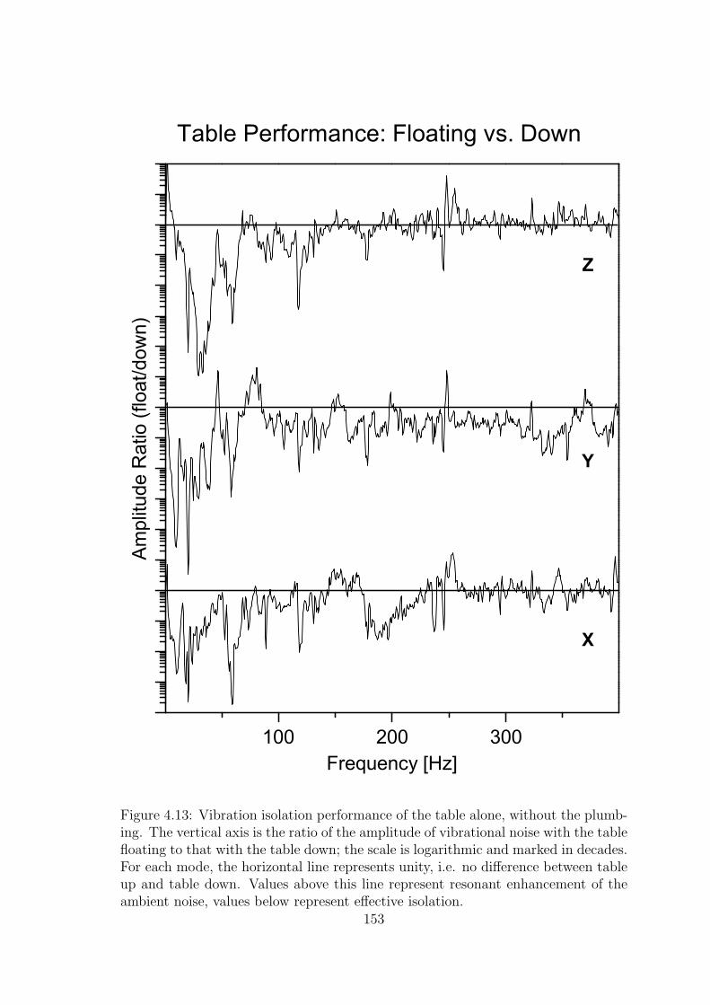
100 200 300
A
mpl
itude
Rat
io (f
loat
/dow
n)
Frequency [Hz]
X
Y
Z
Table Performance: Floating vs. Down
Figure 4.13: Vibration isolation performance of the table alone, without the plumb-ing. The vertical axis is the ratio of the amplitude of vibrational noise with the tablefloating to that with the table down; the scale is logarithmic and marked in decades.For each mode, the horizontal line represents unity, i.e. no difference between tableup and table down. Values above this line represent resonant enhancement of theambient noise, values below represent effective isolation.
153
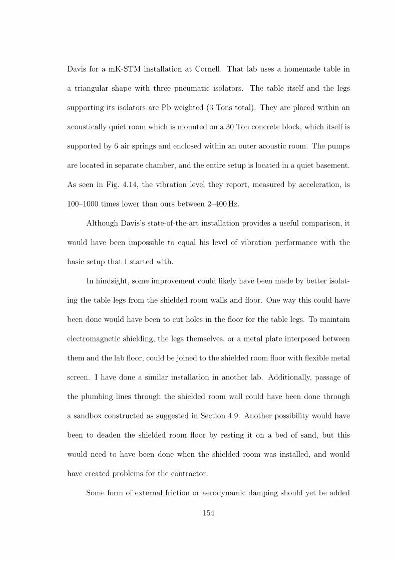
Davis for a mK-STM installation at Cornell. That lab uses a homemade table in
a triangular shape with three pneumatic isolators. The table itself and the legs
supporting its isolators are Pb weighted (3 Tons total). They are placed within an
acoustically quiet room which is mounted on a 30 Ton concrete block, which itself is
supported by 6 air springs and enclosed within an outer acoustic room. The pumps
are located in separate chamber, and the entire setup is located in a quiet basement.
As seen in Fig. 4.14, the vibration level they report, measured by acceleration, is
100–1000 times lower than ours between 2–400 Hz.
Although Davis’s state-of-the-art installation provides a useful comparison, it
would have been impossible to equal his level of vibration performance with the
basic setup that I started with.
In hindsight, some improvement could likely have been made by better isolat-
ing the table legs from the shielded room walls and floor. One way this could have
been done would have been to cut holes in the floor for the table legs. To maintain
electromagnetic shielding, the legs themselves, or a metal plate interposed between
them and the lab floor, could be joined to the shielded room floor with flexible metal
screen. I have done a similar installation in another lab. Additionally, passage of
the plumbing lines through the shielded room wall could have been done through
a sandbox constructed as suggested in Section 4.9. Another possibility would have
been to deaden the shielded room floor by resting it on a bed of sand, but this
would need to have been done when the shielded room was installed, and would
have created problems for the contractor.
Some form of external friction or aerodynamic damping should yet be added
154
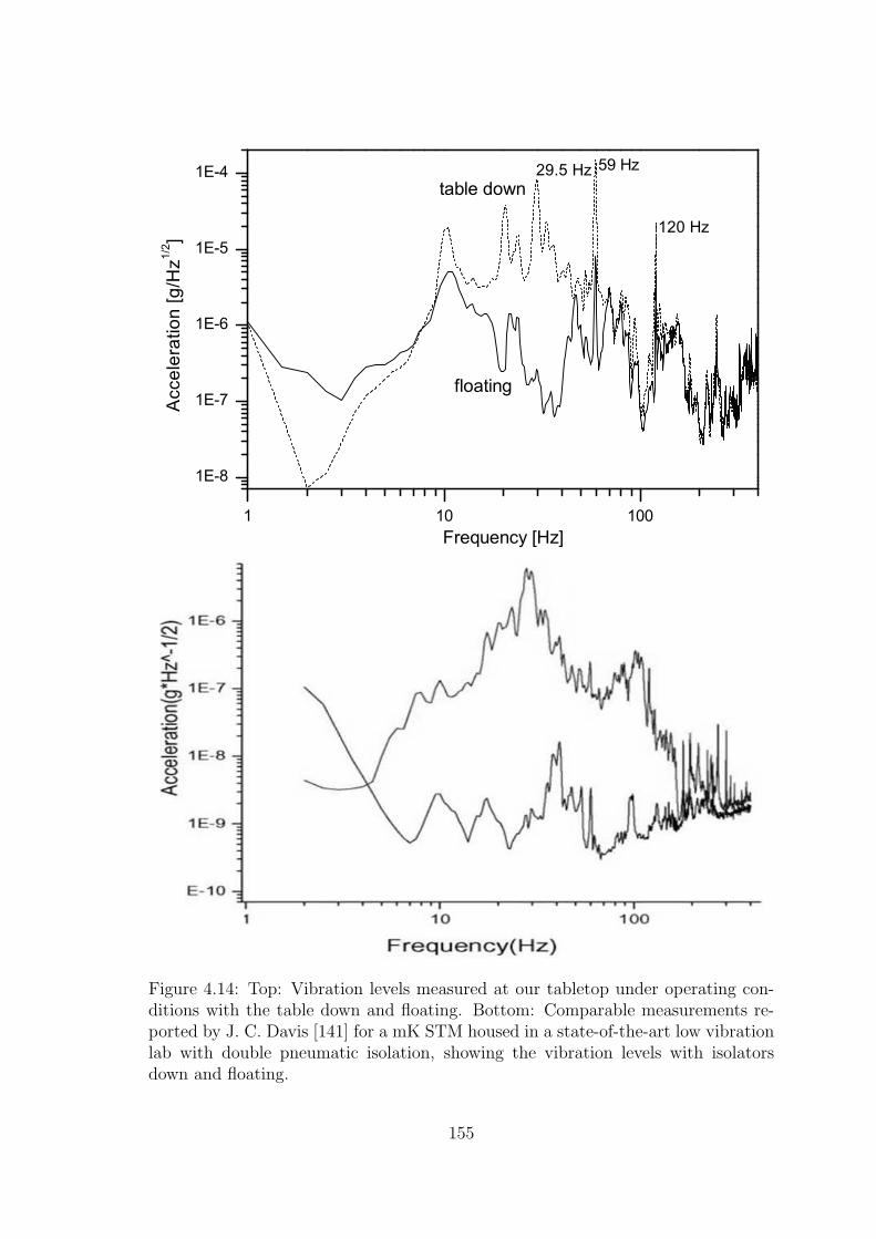
1 10 100
1E-8
1E-7
1E-6
1E-5
1E-4A
ccel
erat
ion
[g/H
z1/2 ]
Frequency [Hz]
59 Hz
120 Hz
29.5 Hztable down
floating
Figure 4.14: Top: Vibration levels measured at our tabletop under operating con-ditions with the table down and floating. Bottom: Comparable measurements re-ported by J. C. Davis [141] for a mK STM housed in a state-of-the-art low vibrationlab with double pneumatic isolation, showing the vibration levels with isolatorsdown and floating.
155
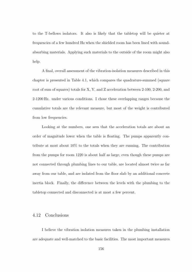
to the T-bellows isolators. It also is likely that the tabletop will be quieter at
frequencies of a few hundred Hz when the shielded room has been lined with sound-
absorbing materials. Applying such materials to the outside of the room might also
help.
A final, overall assessment of the vibration-isolation measures described in this
chapter is presented in Table 4.1, which compares the quadrature-summed (square
root of sum of squares) totals for X, Y, and Z acceleration between 2-100, 2-200, and
2-1200 Hz. under various conditions. I chose these overlapping ranges because the
cumulative totals are the relevant measure, but most of the weight is contributed
from low frequencies.
Looking at the numbers, one sees that the acceleration totals are about an
order of magnitude lower when the table is floating. The pumps apparently con-
tribute at most about 10% to the totals when they are running. The contribution
from the pumps for room 1220 is about half as large, even though these pumps are
not connected through plumbing lines to our table, are located almost twice as far
away from our table, and are isolated from the floor slab by an additional concrete
inertia block. Finally, the difference between the levels with the plumbing to the
tabletop connected and disconnected is at most a few percent.
4.12 Conclusions
I believe the vibration isolation measures taken in the plumbing installation
are adequate and well-matched to the basic facilities. The most important measures
156
Plumbing connected x x x
Table floating x x x x x
1224 Pumps running x x x
1220 Pumps running x
Mode Freq. range µm/s2 µm/s2 µm/s2 µm/s2 µm/s2 µm/s2 µm/s2
2-100 Hz 1869 1935 126 146 130 142 131
Z 2-200 Hz 1883 1949 141 160 144 156 146
2-1200 Hz 1886 1953 194 212 205 208 202
2-100 Hz 414 483 46 52 35 30 -
Y 2-200 Hz 429 497 54 59 41 44 -
2-1200 Hz 445 513 116 118 116 143 -
2-100 Hz 502 589 25 26 25 27 -
X 2-200 Hz 519 604 39 39 35 40 -
2-1200 Hz 541 626 119 115 133 157 -
Table 4.1: Summary of vibration measurements taken at the tabletop, near the axisof the fridge and STM, under various conditions as indicated by the matrix at top.Each measured value is the quadrature sum of acceleration components measuredwithin the indicated (cumulative) frequency ranges. It is seen that the verticalcomponent (Z mode) is a factor of four larger than the horizontal components whenthe table is not floated, and a factor of 2-3 larger in other cases. Floating the tablereduces the acceleration in the range 2-100 Hz by an order of magnitude, roughlyas promised by the manufacturer. Connecting the plumbing lines has only a smalleffect on the totals, and even seeems to decrease the Y component at low frequencies,while increasing the X and Y components at higher frequencies. Similarly, the effectof turning the pumps on is small, and there is not much difference between the caseswhere the pumps for lab 1224 are running and when the 1220 pumps are running.Thus, the level of isolation achieved for the pumps and pumping lines is adequatefrom the perspective that their contribution to the totals is much less than thevibration level of the table itself as installed in the lab.
157

were the use of rubber pads to reduce transmission of vibration from the pumps
to the floor slab, the concreting of pipes into the masonry wall of the pump room,
and the T-bellows isolation of the plumbing lines to the tabletop. More elaborate
measures to isolate the pumps and plumbing lines might have reduced their con-
tribution to the tabletop vibration level, but this contribution is less than 10% of
square-integrated acceleration in the frequency range 2–1200 Hz. The tabletop vi-
bration level appears to have been determined primarily by the effectiveness of the
pneumatic isolation system of the optical table system itself, and by the level of
ambient vibration of the shielded room floor and walls. The sandbox was probably
unnecessary, but would have been more effective if built right against the shielded
room wall.
158
Chapter 5
Mounting the STM and Wiring the Cryostat
In this chapter I describe the design and construction of the STM mount,
which extends downward from the cold plate of the dilution refrigerator and places
the STM in the center of the high-field magnet. I then describe the cryostat wiring
which enters the vacuum space at the top of the cryostat and connects to the STM,
thermally anchored and filtered at the various stages of cooling along the way. I
describe the design and construction of two kinds of filters against radio frequency
(rf) energy which are used at the coldest stage. I also describe a magnetically
shielded sample mount which was used for experiments toward the development of
Josephson phase STM [142].
5.1 STM mount
The STMs that have been used in the LPS 4 K STM lab [126] are derived from
designs developed at Berkeley by Seamus Davis and Shu-Heng Pan [44]. A principal
modification from the Pan–Davis design is that the STM is suspended from a metal
flange at its top, rather than resting on a cold plate.
The STM body is made of Macor, a machinable ceramic. An advantage of
using a ceramic material for the STM body is that its thermal expansion coefficient,
particularly at low temperature, is very small, as are those of the lead zirconium ti-
159
tanate (PZT) scanner tube and of the sapphire prism used in the walker mechanism.
These components comprise the figure “G” loop of the STM, and their differential
expansion and contraction due to temperature drift would be disastrous, particularly
for the ability to hold the tip at constant height without feedback during spectro-
scopic measurements. A disadvantage of Macor, relative to metallic materials, is its
very low thermal conductivity, implying a long cooldown time before stabilization,
and a need for the tip, sample and piezos to be cooled through the wiring.
The STM mount was designed to accomodate a single-tip STM which is a
legacy from the LPS 4 K STM, and to also accomdate a new dual-tip design intended
for use either in Josephson phase STM [142] or for independent dual-tip operation of
the STM. The body of the dual-tip STM is longer and wider in order to accomodate
two stacked, independent, Pan-type walker mechanisms [43] and two concentric piezo
scanner tubes.
The overall configuration of the STM mount is shown in Figure 5.1. The Ma-
cor STM body is bolted to a Cu flange, with bolt patterns provided for both the
single and dual-tip STM designs. The STM mounting flange is suspended inside a
Cu can for electrical shielding. The can is 7 in. long × 2.3 in. OD, and is designed
to fit inside the tailpiece of the 100 mK radiation shield without touching. Three
2.5 in. long × 1
4in. square Cu rods suspend the STM mounting flange from the Cu
top flange of the STM shielding can. The shielding can top flange is in turn sus-
pended by three 11.7 in. long × 1
4in. × 1
2in. rectangular Cu bars, which are bolted
to the mixing chamber cold plate.
All these main Cu parts of the STM mount are Au-plated to promote thermal
160
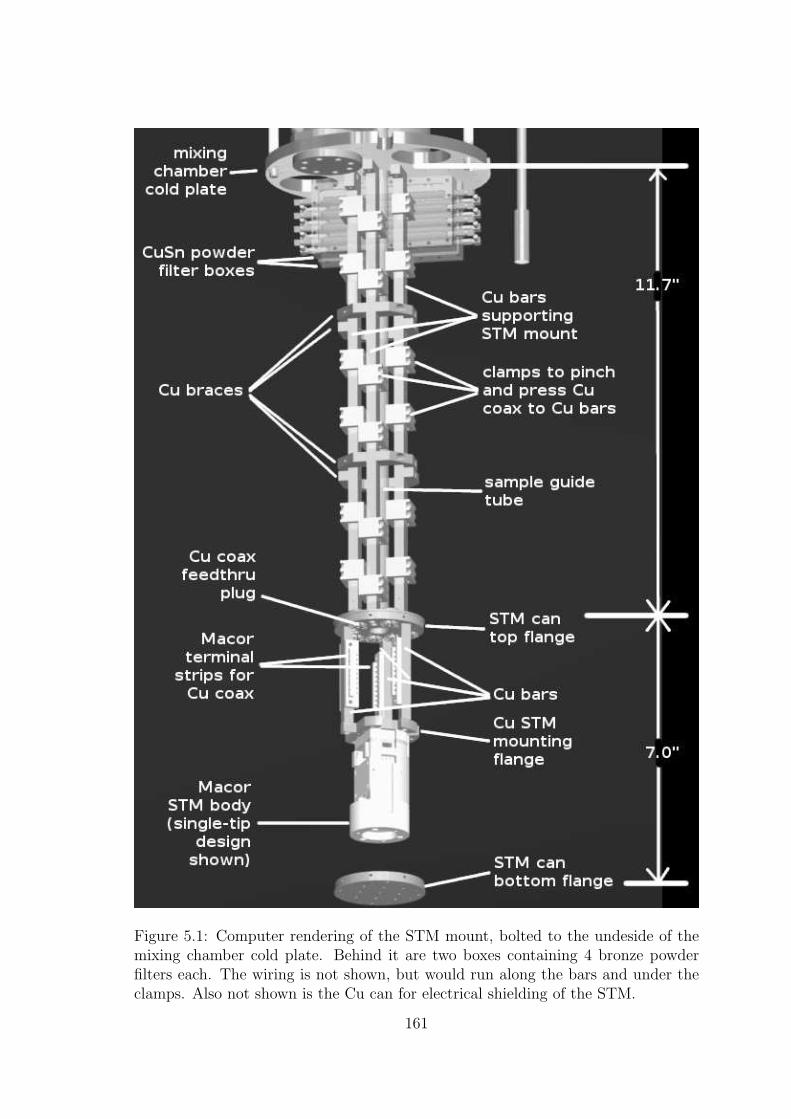
Figure 5.1: Computer rendering of the STM mount, bolted to the undeside of themixing chamber cold plate. Behind it are two boxes containing 4 bronze powderfilters each. The wiring is not shown, but would run along the bars and under theclamps. Also not shown is the Cu can for electrical shielding of the STM.
161
contact to each other and to the Au-plated Cu cold plate of the fridge. The 11.7 in.
long upper bars are bolted to the cold plate by two M3 cap screws each, and their
top ends are extended in an “L” shape to facilitate this, since the bolt holes on the
cold plate are spaced 0.59 in. (15 mm) apart. At the lower end of the bars, they are
bolted to the top flange of the can by two UNC 4-40 cap screws. The three shorter
bars suspending the STM mounting flange inside the can are attached with single
4-40 cap screws threaded into their ends.
The three 11.7 in. long bars could not be arranged in an equilateral triangle
due to space constraints imposed by the design of the fridge. Instead, two bars are
approximately coplanar with the axis, on opposite sides of it, with the third bar in
front (as viewed in Fig. 5.1). This geometry is inherently less stiff in the front-back
direction than in the right-left. Making the bars rectangular in cross-section, with
the long side running front-back, compensates for this weakness. In addition, two
sets of Cu braces are bolted between the three bars, pinning their lowest internal
vibrational modes and stiffening the assembly.
A 1
2in. OD Cu tube is soft-soldered into the top flange of the STM can, on
its axis, and runs up to the mixing chamber cold plate where it is to be sealed by
an rf-tight shutter (not yet developed). This tube provides access to the STM for
sample and tip exchange, and guides the exchange rod. It is thermally anchored at
the mixing chamber cold plate via a Cu clamp which is bolted to the plate, although
the cooling of this tube is not critical.
As discussed in Sec. 3.2, the bolts should be as tight as possible for good
thermal contact. We had originally specified the use of Ti bolts on the STM mount
162
in order to avoid magnetic materials, due to our interest in Josephson phase STM.
However, Ti has quite small thermal contraction, ∆ℓ/ℓ = 0.151% between RT and
4 K, compared with 0.324% for Cu [4]. This 0.15% difference is 6× greater than
when using stainless steel bolts [4].
The maximum recommended load on a 4-40 stainless steel bolt into Al is
0.8 kN [4], and the shear strength of Cu is about the same as Al. Ti is stronger than
stainless steel, but my experience is that an overtightened stainless steel screw into
Cu will strip the Cu threads before breaking the screw. Therefore I assume a similar
rating for a 4-40 Ti bolt into Cu. The cross sectional area of the bolt is ∼4 mm2, and
the Young’s modulus of Ti alloys is ∼110 GPa. Based on these numbers, we expect
stretching of up to about 0.18% when the Ti bolts are tightened at RT. Comparing
this with the 0.15% differential thermal contraction, we see that the Ti bolts would
loosen substantially or completely when cold.
For this reason, it is probably better to use ZnCu brass bolts, which have
∆ℓ/ℓ = 0.38%, slightly greater than that of Cu. Although Ti is as much as 5 times
stronger than ZnCu, the factor limiting tightness of the bolts is more likely the Cu
threads. Since the brass bolts will tighten slightly on cooling, they should not be
overtightened.
163
5.2 Cryostat wiring
5.2.1 General requirements
STM and STS at millikelvin temperatures normally require only low-frequency
(dc to about 20 kHz) electrical connections between the STM inside the cryostat
and the external instrumentation at room temperature. However, the wiring must
satisfy a number of demanding and sometimes conflicting criteria. Lengthwise ther-
mal conduction must not impose an excessive heat load on the refrigeration, but
reasonably low-resistance electrical connections must be provided from room tem-
perature down to the STM. Thermal anchoring must be provided at each stage of
cooling in order not to impose excessive heat loads on the colder stages, but electrical
insulation must be maintained.
Since tunneling resistances are typically up to 1 GΩ and might be as high as
300 GΩ, the tip and sample wires must be very well insulated. The insulation must
be able to withstand up to ∼200 V which is periodically applied to clean the tip by
field emission. Capacitance must also be limited to minimize the noise current due
to noise voltage present on the input of the transimpedance preamplifier.
Since the STM body is generally made of an insulating material (Macor in our
case), the wires must carry away and sink the bulk of any heat dissipated due to
the tunneling current or due to the operation of the piezos.
Achieving the lowest physical temperatures at the tip-sample junction, and
the lowest effective temperatures in spectroscopy, requires shielding and filtering to
exclude ambient rf signals and noise generated by the instrumentation and wiring at
164
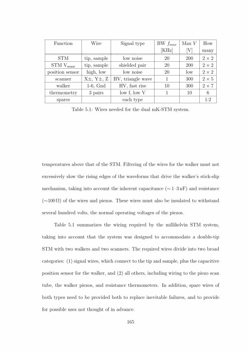
Function Wire Signal type BW fmax Max V How
[KHz] [V] many
STM tip, sample low noise 20 200 2 × 2
STM Vsense tip, sample shielded pair 20 200 2 × 2
position sensor high, low low noise 20 low 2 × 2
scanner X±, Y±, Z HV, triangle wave 1 300 2 × 5
walker 1-6, Gnd HV, fast rise 10 300 2 × 7
thermometry 3 pairs low f, low V 1 10 6
spares each type 1:2
Table 5.1: Wires needed for the dual mK-STM system.
temperatures above that of the STM. Filtering of the wires for the walker must not
excessively slow the rising edges of the waveforms that drive the walker’s stick-slip
mechanism, taking into account the inherent capacitance (∼ 1–3 nF) and resistance
(∼100 Ω) of the wires and piezos. These wires must also be insulated to withstand
several hundred volts, the normal operating voltages of the piezos.
Table 5.1 summarizes the wiring required by the millikelvin STM system,
taking into account that the system was designed to accommodate a double-tip
STM with two walkers and two scanners. The required wires divide into two broad
categories: (1) signal wires, which connect to the tip and sample, plus the capacitive
position sensor for the walker, and (2) all others, including wiring to the piezo scan
tube, the walker piezos, and resistance thermometers. In addition, spare wires of
both types need to be provided both to replace inevitable failures, and to provide
for possible uses not thought of in advance.
165
5.2.2 Signal wires
The signal wires are those particularly in need of shielding and low, stable
capacitance, and include the STM tip and sample wires, and the capacitive tip
position sensor wires. All of these wires are driven by low-impedance instruments
at the warm end, and their cold end terminations are usually high-impedance. The
tunneling current is very small, and as a result its measurement will be very sensitive
to charge induced by electric coupling from noise sources.
For normal STM with two independent tips, a minimal wiring scheme would
require three signal wires (Fig. 5.2 A): one for the sample, plus one for each tip. The
sample wire would conventionally carry the bias voltage, and each tip wire would
conventionally drain into a transimpedance amplifier (current-voltage converter).
Each transimpedance amplifier acts as a virtual ground, i.e. an active device that
supplies current as needed in order to maintain its input at some set potential, which
might be the environmental ground potential, or might be a different setpoint. In
some experiments, each tip might be set at a different potential.
Somewhat more complicated wiring schemes may provide better performance.
Zuger et al. [143] used separate twisted pairs to carry differential tip and sample
signals referenced to a common local ground at the STM body (Fig. 5.2 B). This
arrangement may be expected to reduce any noise from potential differences between
the instrumentation and the local (cold) environment, which might couple unequally
to the tip and sample.
le Sueur and Joyez [144, 109] demonstrated a dramatic reduction in voltage
166
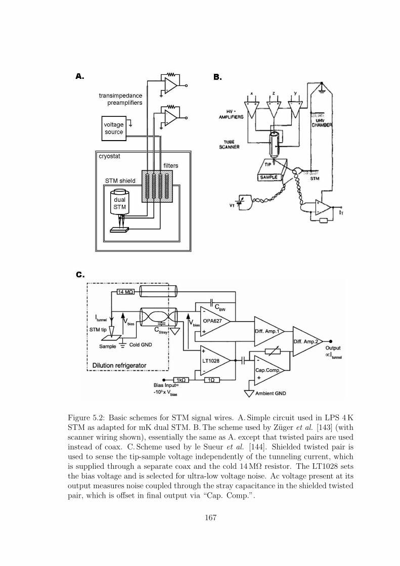
Figure 5.2: Basic schemes for STM signal wires. A. Simple circuit used in LPS 4 KSTM as adapted for mK dual STM. B. The scheme used by Zuger et al. [143] (withscanner wiring shown), essentially the same as A. except that twisted pairs are usedinstead of coax. C. Scheme used by le Sueur et al. [144]. Shielded twisted pair isused to sense the tip-sample voltage independently of the tunneling current, whichis supplied through a separate coax and the cold 14 MΩ resistor. The LT1028 setsthe bias voltage and is selected for ultra-low voltage noise. Ac voltage present at itsoutput measures noise coupled through the stray capacitance in the shielded twistedpair, which is offset in final output via “Cap. Comp.”.
167
noise, and hence improved spectroscopic resolution, by using a twisted pair in par-
allel with the tunneling current wires to sense the voltage between tip and sample
(Fig. 5.2 C). Additionally, the transimpedance feedback resistor, through which the
tunneling current flows, was mounted on the cold STM to reduce Johnson noise in
the resistor, while keeping the active devices of the preamp at room temperature.
They claimed that this cold resistor–warm amplifier arrangement provided most of
the benefits of a cold transimpedance preamp, while avoiding the difficulties of the
latter, and that the result was a spectroscopic effective temperature of ∼45 mK,
very close to their sample temperature, and much better than previous efforts using
conventional electronics and wiring.
At least one commercial supplier [145] provides CuNi braid-shielded twisted
pair wiring, including superconducting NbTi and, for connection to RT, brass con-
ductor versions. In combination with CuNi or stainless steel tubing to provide better
shielding after low temperature filtering, this might be a good option for providing
voltage-sense pairs or other situations where elimination of magnetically coupled
noise is critical.
For the proposed Josephson phase STM [142], two superconducting tips would
be joined by a flexible superconducting wire, which with tunneling to a supercon-
ducting sample would form a SQUID. In this approach, there would be only one
tip-sample voltage. In the originally-proposed scheme, a two-wire measurement
would be adequate, but another possible approach would likely benefit from four-
wire measurement to reduce noise. Phase STM may also require additional signal
wires. In particular, it would probably need at least one pair for a magnetic feed-
168
back coil. This would be a low-impedance circuit, carrying a relatively high current
(µA), but it would probably need to be well-shielded from noise sources.
To provide for these possible configurations, and in order to have spare wires
available in case of failures, I chose to route 12 wires as signal wires. The number
should be sufficient for the schemes considered here, but a somewhat larger number
of spares might be desirable.
We do not need to worry about impedance matching and rf propagation in
these wires. Actually, we want to block rf as much as possible, and reflection caused
by impedance mismatch is one mechanism which can contribute to this [110]. Re-
flections will not appreciably degrade the signal quality at 20 kHz, since the path
length from the STM to the preamplifier is at most a few meters.
However, the STM signal wires need to be well-shielded to exclude rf as well
as low-frequency electrical noise. Another possible noise source is magnetic pickup
due to 60 Hz fields and, when the high-field magnet is used, vibration of the wire
or of nearby magnetic parts through the field.
Experience has shown [146] that one of the most troublesome noise sources
in low temperature STM is microphonic pickup of ambient sound by coaxial ca-
bles used for the STM signal wires. The measured quantity is usually current (and
its derivatives) in the range of 10−11–10−7 A. Since 2 m of 50 Ω coaxial cable will
typically have about 200 pF of capacitance, if it is charged to 1 V and if the ca-
pacitance changes by a factor of 1+10−4, the charge dislodged will be equivalent
to 200 pA for 0.1 ms, for example. Motion of the cables may also release charge
through piezoelectric or triboelectric effects.
169
Whatever the mechanism, the braid-shielded teflon coax used in the 4 K STM
at LPS is apparently quite sensitive to sound. Semi-rigid coax (continuous metal
shield) is much stiffer and should be less microphonic. Semi-rigid coax is also far
better shielded against rf pickup, which is particularly important for the cable be-
tween the STM and the cold filters. It can be joined with rf connectors which are
also quite rf-tight.
For these reasons, I used semi-rigid coax for all signal wires inside the vacuum
space of the cryostat. To minimize the thermal load, and to provide some rf atten-
uation, I used resistive coax made of CuNi (375nΩm @ RT[115]) inner and outer
conductor and PTFE dielectric [115]. The 0.4 mm diam. micro-coax has shield
inner diameter 0.26 mm and wire (inner conductor) diameter 0.08 mm, for a total
cross-section of CuNi A = 8×10⁻⁸ m2. Using the data of Olson [55] (Table 3.1),
the heat leak through a length ℓ of the CuNi coax connecting a thermal anchor at
temperature T1 to the next higher anchor at temperature T2 is given by
Q =A
ℓ
∫ T2
T1
κ(T ) dT =A
ℓ
∫ T2
T1
0.065
(
T
K
)1.1W
md
(
T
K
)
=A
ℓ· 0.031 ·
[(
T2
K
)2.1
−(
T1
K
)2.1 ]
W
m. (5.1)
We are most interested in knowing the heat leak to the mixing chamber cold plate.
The next higher anchor is at the radiation shield cold plate, which is nominally at
50 mK. However, there is no cooling power at this stage; the radiation shield is cooled
below the still temperature by the mixing chamber. Therefore it is appropriate to
compute the total heat leak from the still, at T2 = 0.7 K, to the mixing chamber at
170
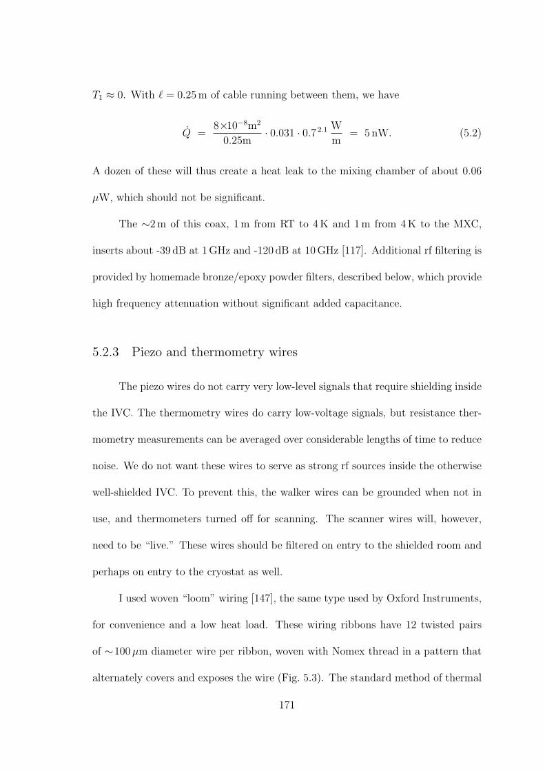
T1 ≈ 0. With ℓ = 0.25 m of cable running between them, we have
Q =8×10⁻⁸m2
0.25m· 0.031 · 0.7 2.1 W
m= 5 nW. (5.2)
A dozen of these will thus create a heat leak to the mixing chamber of about 0.06
µW, which should not be significant.
The ∼2 m of this coax, 1 m from RT to 4 K and 1 m from 4 K to the MXC,
inserts about -39 dB at 1 GHz and -120 dB at 10 GHz [117]. Additional rf filtering is
provided by homemade bronze/epoxy powder filters, described below, which provide
high frequency attenuation without significant added capacitance.
5.2.3 Piezo and thermometry wires
The piezo wires do not carry very low-level signals that require shielding inside
the IVC. The thermometry wires do carry low-voltage signals, but resistance ther-
mometry measurements can be averaged over considerable lengths of time to reduce
noise. We do not want these wires to serve as strong rf sources inside the otherwise
well-shielded IVC. To prevent this, the walker wires can be grounded when not in
use, and thermometers turned off for scanning. The scanner wires will, however,
need to be “live.” These wires should be filtered on entry to the shielded room and
perhaps on entry to the cryostat as well.
I used woven “loom” wiring [147], the same type used by Oxford Instruments,
for convenience and a low heat load. These wiring ribbons have 12 twisted pairs
of ∼100 µm diameter wire per ribbon, woven with Nomex thread in a pattern that
alternately covers and exposes the wire (Fig. 5.3). The standard method of thermal
171
Figure 5.3: Wiring and thermal anchoring methods used for the signal and piezowires inside the IVC. A. CuNi microcoaxes used as signal wires at with SSMC con-nectors and thermal anchors at 4 K flange (hanging from top) and thermal anchorsat 1 K plate (bottom). 0.4 mm OD microcoaxes are bunched beneath the squareplates into 0.3 mm deep channels to compress them for thermal contact. B. NbTiloom wiring between 1 K plate and 50 mK plate. 1.5 in. long Cu thermal anchoringposts are used at the 600 mK still stage, and 3 in. long posts are used at the 50 mKshield stage.
172
anchoring of loom wiring, used by Oxford, is to wind them around 1
4in. OD Cu
posts. When the ribbon is wrapped around a heatsinking post, exposed sections of
the wires come into contact with the post, and thermal contact can be enhanced by
using varnish as a bonding agent.
For the upper section running from 300 K down to the 1.4 K stage, I used
110 µm diameter Constantan wiring loom. This choice provides a low heat load
at the cost of somewhat high electrical resistance, 66 Ω/m, with little variation of
resistance (hence the name “Constantan”) due to temperature changes as liquid
helium is depleted or when refilling.
For the lower section running from 1.4 K down to the mixing chamber, I used
CuNi-clad NbTi loom, 100µm diameter, which has room temperature resistance
52 Ω/m but is superconducting below about 9 K. The CuNi cladding is mainly for
solderability. Transmission of microwave energy is also suppressed by the resistive
cladding due to the skin effect and capacitance between the twisted pairs, while dc
resistance (when cold) is zero.
The heat leak to the mixing chamber due to the CuNi-clad NbTi wiring is
almost entirely through the CuNi. Although the amount of the CuNi is not spec-
ified by the supplier, the wire diameter is specified as 100µm, and similar wire
made by Supercon, Inc. (type SW-M) [148] contains 62µm of NbTi with the bal-
ance CuNi. Assuming this is the correct proportion (1.5:1 area proportion of ma-
trix to superconductor appears to be standard), the area of CuNi for 48 wires is
2.3×10⁻⁷m2. Comparison with the calculation done for the CuNi coax (above)
shows an expected heat leak of 12 nW, which is insignificant.
173
Oxford Instruments conventionally wraps loom wiring around 25 mm long,
6 mm diameter Cu posts, which are hollow and are bolted to the cold plates with
long stainless steel screws. They tie down the loom with thread and apply varnish
to provide additional thermal contact to the post. While this method appears to be
adequate for the upper stages of a dilution fridge, my experience has been that the
wires are not adequately thermalized at the mixing chamber.
To ensure adequate thermal anchoring of the looms, I used extra-long heat
sinking posts: 40 mm at the 4 K, 1 K, and 0.7 K stages, and 75 mm at the 50mK
shield stage and at the mixing chamber (Fig. 5.3). These posts were also threaded
and screwed directly into the cold plates for better contact. Holes drilled horizontally
into the posts allowed them to be tightened with a steel bar (actually, a small Allen
wrench). Bending of the bar was used to gauge the tightening torque so that the
posts could be put in as tightly as possible without breaking.
Although 48 total wires are brought down on two looms, 12 of these are treated
as spares and left open at the mixing chamber. The 36 remaining wires are to be
filtered at the mixing chamber, and shielded after filtering until they enter the
STM can. I planned to use Thermocoax wound on spools to filter the piezo and
thermometry wires. Due to difficulties with this type of filter, it may be desirable to
use a different filtering element at this stage, but I describe the Thermocoax filter
design below.
174
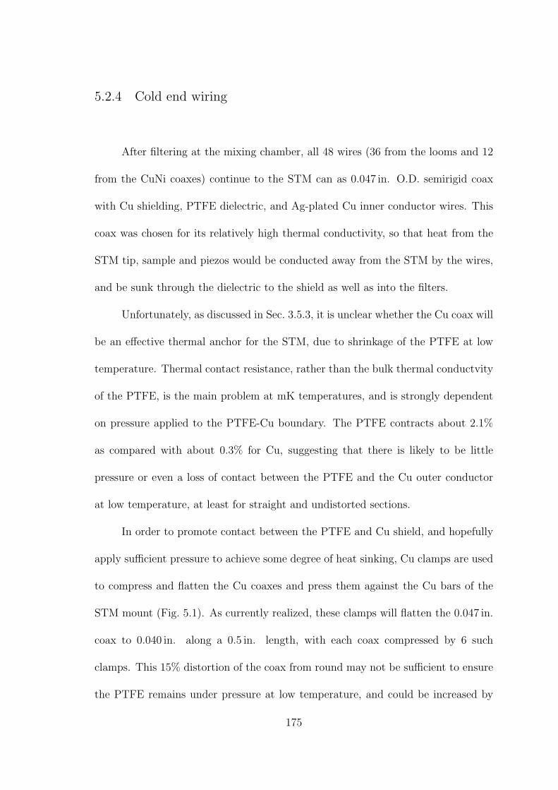
5.2.4 Cold end wiring
After filtering at the mixing chamber, all 48 wires (36 from the looms and 12
from the CuNi coaxes) continue to the STM can as 0.047 in. O.D. semirigid coax
with Cu shielding, PTFE dielectric, and Ag-plated Cu inner conductor wires. This
coax was chosen for its relatively high thermal conductivity, so that heat from the
STM tip, sample and piezos would be conducted away from the STM by the wires,
and be sunk through the dielectric to the shield as well as into the filters.
Unfortunately, as discussed in Sec. 3.5.3, it is unclear whether the Cu coax will
be an effective thermal anchor for the STM, due to shrinkage of the PTFE at low
temperature. Thermal contact resistance, rather than the bulk thermal conductvity
of the PTFE, is the main problem at mK temperatures, and is strongly dependent
on pressure applied to the PTFE-Cu boundary. The PTFE contracts about 2.1%
as compared with about 0.3% for Cu, suggesting that there is likely to be little
pressure or even a loss of contact between the PTFE and the Cu outer conductor
at low temperature, at least for straight and undistorted sections.
In order to promote contact between the PTFE and Cu shield, and hopefully
apply sufficient pressure to achieve some degree of heat sinking, Cu clamps are used
to compress and flatten the Cu coaxes and press them against the Cu bars of the
STM mount (Fig. 5.1). As currently realized, these clamps will flatten the 0.047 in.
coax to 0.040 in. along a 0.5 in. length, with each coax compressed by 6 such
clamps. This 15% distortion of the coax from round may not be sufficient to ensure
the PTFE remains under pressure at low temperature, and could be increased by
175
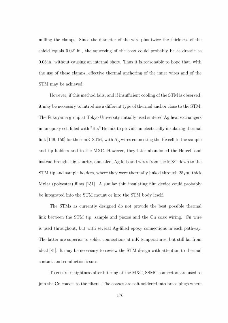
milling the clamps. Since the diameter of the wire plus twice the thickness of the
shield equals 0.021 in., the squeezing of the coax could probably be as drastic as
0.03 in. without causing an internal short. Thus it is reasonable to hope that, with
the use of these clamps, effective thermal anchoring of the inner wires and of the
STM may be achieved.
However, if this method fails, and if insufficient cooling of the STM is observed,
it may be necessary to introduce a different type of thermal anchor close to the STM.
The Fukuyama group at Tokyo University initially used sintered Ag heat exchangers
in an epoxy cell filled with 3He/4He mix to provide an electrically insulating thermal
link [149, 150] for their mK-STM, with Ag wires connecting the He cell to the sample
and tip holders and to the MXC. However, they later abandoned the He cell and
instead brought high-purity, annealed, Ag foils and wires from the MXC down to the
STM tip and sample holders, where they were thermally linked through 25µm thick
Mylar (polyester) films [151]. A similar thin insulating film device could probably
be integrated into the STM mount or into the STM body itself.
The STMs as currently designed do not provide the best possible thermal
link between the STM tip, sample and piezos and the Cu coax wiring. Cu wire
is used throughout, but with several Ag-filled epoxy connections in each pathway.
The latter are superior to solder connections at mK temperatures, but still far from
ideal [81]. It may be necessary to review the STM design with attention to thermal
contact and conduction issues.
To ensure rf-tightness after filtering at the MXC, SSMC connectors are used to
join the Cu coaxes to the filters. The coaxes are soft-soldered into brass plugs where
176
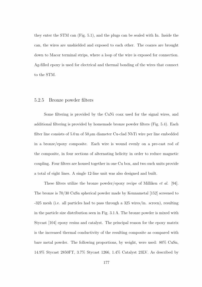
they enter the STM can (Fig. 5.1), and the plugs can be sealed with In. Inside the
can, the wires are unshielded and exposed to each other. The coaxes are brought
down to Macor terminal strips, where a loop of the wire is exposed for connection.
Ag-filled epoxy is used for electrical and thermal bonding of the wires that connect
to the STM.
5.2.5 Bronze powder filters
Some filtering is provided by the CuNi coax used for the signal wires, and
additional filtering is provided by homemade bronze powder filters (Fig. 5.4). Each
filter line consists of 5.0 m of 50µm diameter Cu-clad NbTi wire per line embedded
in a bronze/epoxy composite. Each wire is wound evenly on a pre-cast rod of
the composite, in four sections of alternating helicity in order to reduce magnetic
coupling. Four filters are housed together in one Cu box, and two such units provide
a total of eight lines. A single 12-line unit was also designed and built.
These filters utilize the bronze powder/epoxy recipe of Milliken et al. [94].
The bronze is 70/30 CuSn spherical powder made by Kennametal [152] screened to
-325 mesh (i.e. all particles had to pass through a 325 wires/in. screen), resulting
in the particle size distribution seen in Fig. 3.1 A. The bronze powder is mixed with
Stycast [104] epoxy resins and catalyst. The principal reason for the epoxy matrix
is the increased thermal conductivity of the resulting composite as compared with
bare metal powder. The following proportions, by weight, were used: 80% CuSn,
14.9% Stycast 2850FT, 3.7% Stycast 1266, 1.4% Catalyst 23LV. As described by
177
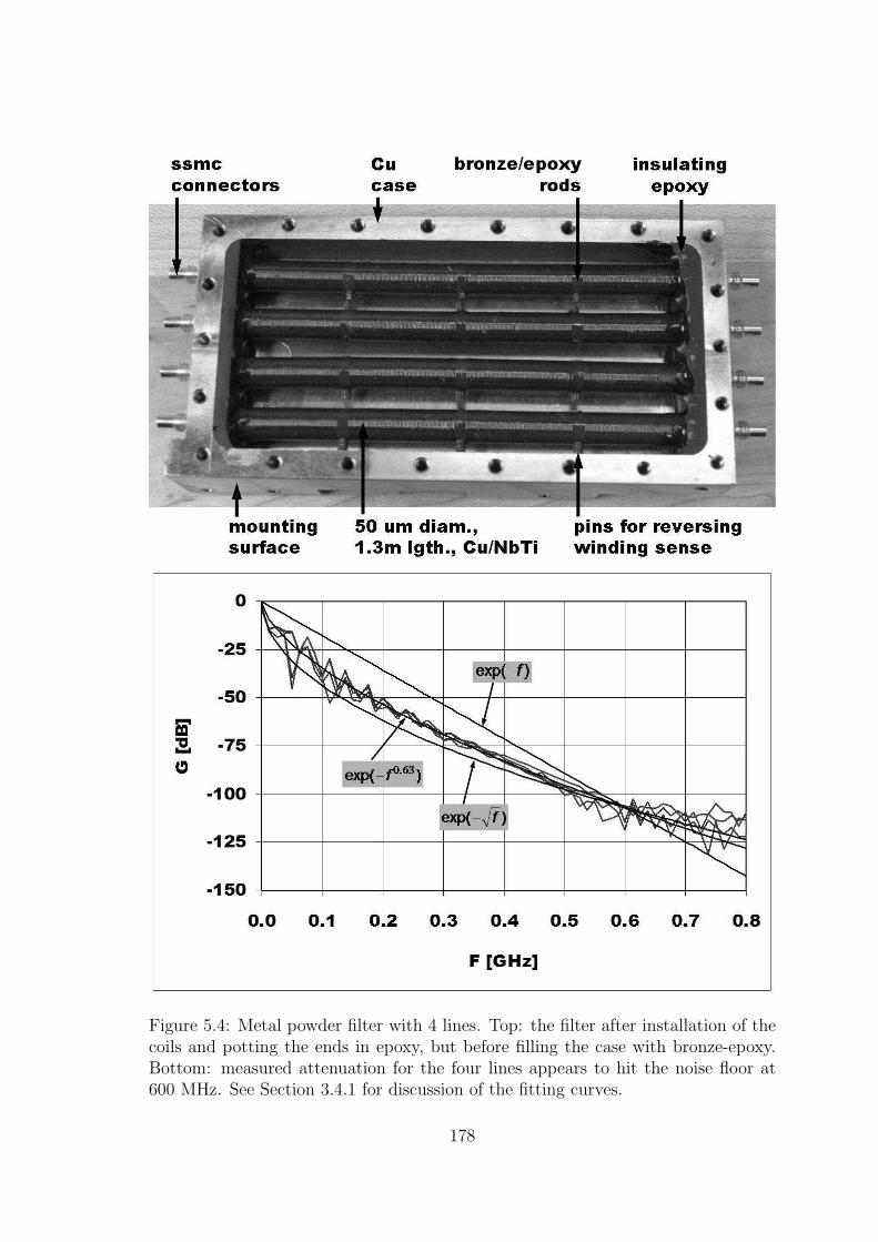
Figure 5.4: Metal powder filter with 4 lines. Top: the filter after installation of thecoils and potting the ends in epoxy, but before filling the case with bronze-epoxy.Bottom: measured attenuation for the four lines appears to hit the noise floor at600 MHz. See Section 3.4.1 for discussion of the fitting curves.
178
Milliken, the addition of unfilled Stycast 1266 to the ceramic-filled 2850FT helps
to reduce cracking, and 23LV is the lowest viscosity catalyst available for use with
these epoxies. The fraction of bronze that can be mixed into the epoxy is limited by
the viscosity of the resulting paste; tests by Milliken et al. showed that attenuation
was highest when the maximum fraction of the mixture was metal.
The epoxy must be mixed very thoroughly, which leaves the paste full of small
air bubbles (Fig. 5.5 E). To remove most of these bubbles, the tray of paste can be
put into a bell jar and pumped to low pressure, causing the air bubbles to expand
and burst. Repeated evacuation and sudden venting of the jar “slaps” the paste and
helps to burst the bubbles. A few cycles of this treatment is apparently enough to
remove most of the air bubbles, which begin expanding immediately as the pressure
was lowered. However, at very low pressure, the mixture seems to boil indefinitely,
probably due to volatile components of the epoxy.
The rods for winding the wires into coils needed to be cast and machined.
Drinking straws with an inner diameter of 5.5 mm were used as mold liners, and the
rods are 79.25 mm long. Early attempts showed that it was necessary to make a
mold, consisting of holes drilled into a block of Teflon, in order to enforce roundness.
A Teflon block was used to cap the bottom end of the mold, but left loose to allow
air to escape. After cutting the straws to length and inserting them in the mold
(Fig. 5.5 A), I filled a 10 ml syringe with the bronze/epoxy paste by removing the
plunger and spooning the paste into the back, taking care to avoid trapping air in
the syringe. I then injected the paste into the straws from the top until it started
to come out the bottom of the mold.
179
Figure 5.5: Some aspects of making powder filters. A. Drinking straws used as moldliners. B. Mixing the bronze/epoxy paste. C. Spooning the paste into a syringe.D. Injecting the paste. E. Bubbles in a test rod. F. Using vacuum to remove bubblesfrom the paste.
180
After allowing the mixture to cure for 24 hours, the bottom cap could be
removed and excess material trimmed off with a razor blade. The rods could then
be pushed out of the mold by using a drill press with a soft plastic rod. The straws
could be scored lengthwise with a razor blade and peeled off. The rods needed to be
cast extra long and then cut to length because of bubbles at the ends. After casting
and cutting, the rods could be weighed and compared to detect any large hidden
bubbles. I obtained a yield of about 2 out of 3 good rods.
I found that the bronze/epoxy composite is initially somewhat soft, and grad-
ually hardens over a period of 1–2 weeks. The best time to machine it is a few days
after casting, before it is fully hard and brittle. The rods have three 1.59 mm holes
drilled across their diameter, dividing them lengthwise into four equal sections. The
holes are used to insert short pegs around which the wire can be wrapped 1
2turn
to reverse the winding sense. Because of the ceramic filler in Stycast 2850FT, the
composite quickly abrades drill bits and other tools used to machine it.
Holes are also drilled into the ends of the rods for short brass sleeves that
mate to pins connecting the wires to the outside (Fig. 5.5). For reasons of electrical
insulation, as described below, I found it necessary to drill these holes wider and
deeper than the brass sleeves, refill them with Stycast 2850FT (without the bronze)
and, after curing, redrill the holes to the correct diameter and depth for the brass
sleeves. The sleeves need to stick out of the ends of the rods by 1.25 mm, just enough
to attach the wires using Ag-filled epoxy. The brass sleeves are also drilled to an
internal diameter of 0.036 in., which makes a gentle press fit over the BeCu soldering
pins of SSMC bulkhead jacks used for connection of the filters to the outside. Since
181
ZnCu brass has greater total thermal contraction (0.384%) than BeCu (0.316%) [4],
contact is maintained at low temperature, and a bit of Ag-filled epoxy is also applied
on the pins for good measure.
The wire was wound on the rods using a small coil winder equipped with a
computer-controlled traverse (Fig. 5.6) used to regulate the spacing, in this case to
250µm per turn. I fitted the traverse with V-grooved Teflon wheels to guide the
fine wire, and used a small weight to regulate tension in the wire. I used plastic
insulation sleeve glued into the rods with cyanoacrylate “super glue” to make pegs
for reversing the winding sense. The wire would be started at one end of the rod with
a drop of cyanoacrylate to attach it, leaving a “pigtail” for connection to the brass
sleeve. Seventy-three turns would be wound in one sense, then the wire wrapped
half a turn around the first peg and fixed in place with cyanocrylate. Then 73
turns in the opposite sense, and repeat for all four sections of the rod (for the final
section, the rod needed to be removed from the winder and turned around so it could
be wound to its end). Finally, the “pigtails” of the wires needed to be chemically
stripped and wound around the protruding brass sleeves. Cyanoacrylate was used to
hold the pigtail in place while the Ag-filled epoxy cured to complete the connection
to the brass sleeves. Of course it was necessary to keep the connections free of the
cyanoacrylate, and to manage to complete all these steps without breaking the 50µm
diameter wire! Although I developed the methods, I thank Anita Roychowdhury
for her patience in finishing the work.
After winding the rods, they were coated with two layers of thinned GE/IMI
7031 varnish, and then installed into the filter boxes. To do this, the SSMC bulkhead
182
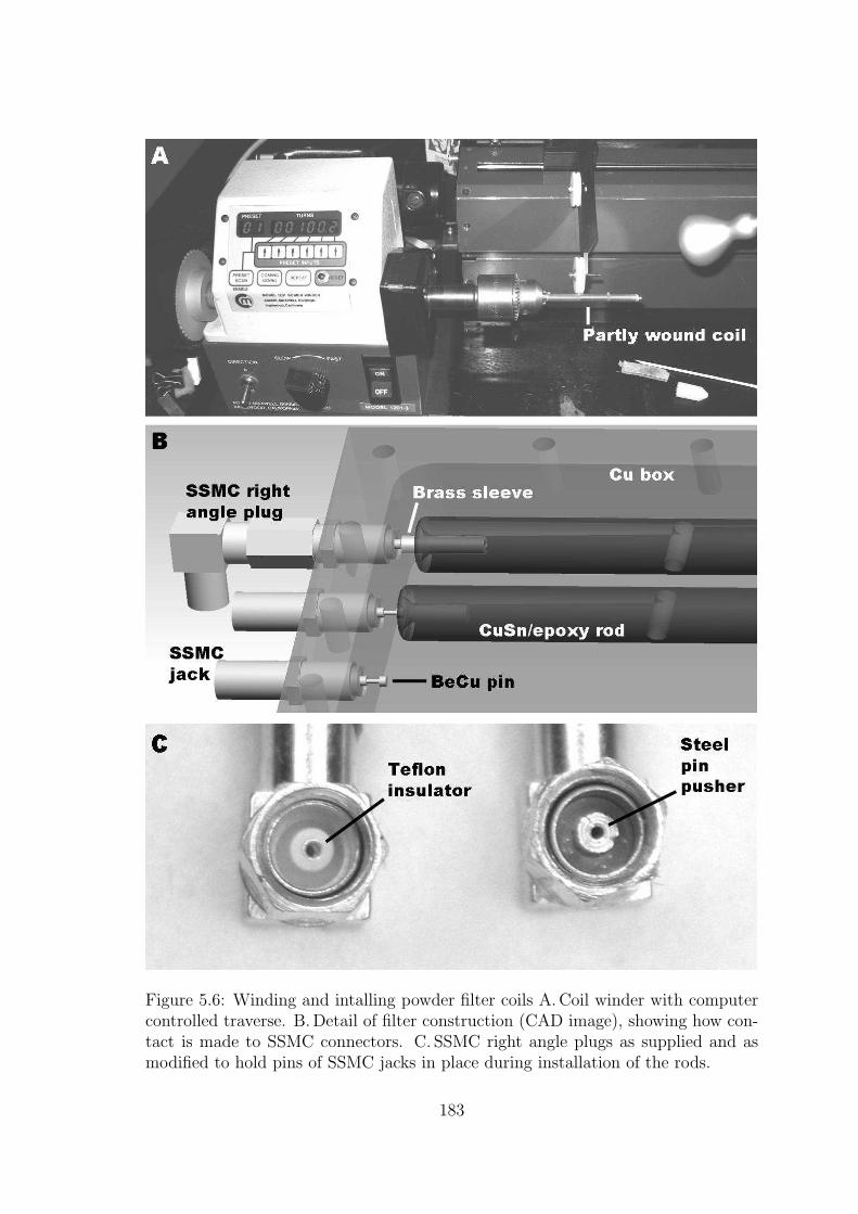
Figure 5.6: Winding and intalling powder filter coils A. Coil winder with computercontrolled traverse. B. Detail of filter construction (CAD image), showing how con-tact is made to SSMC connectors. C. SSMC right angle plugs as supplied and asmodified to hold pins of SSMC jacks in place during installation of the rods.
183
jack connectors (Fig. 5.5) were pre-installed part way in their threaded holes on both
sides of a rod, then slowly tightened to push the pins into the brass sleeves, checking
to ensure they inserted evenly on both ends. Unfortunately, due to the construction
of the SSMC bulkhead jacks, I found that instead of inserting into the sleeves the
pins would push out of the jacks as the latter were tightened down. To solve this
problem, I modified two SSMC right angle plugs with machined stainless steel “pin
pushers” (Fig. 5.6)
The metal particles have a native oxide layer which causes the powder to
appear electrically insulating when tested at low voltage, e.g. by dipping the probes
of an ohmmeter into the powder. The presence of such an oxide layer on the surface
of metal objects is normally unnoticed because it is so easily scraped through by
the touch of another piece of metal, such as an ohmmeter probe. In the case of the
powder, the oxide would have to be scraped through on many contiguous particles,
and not re-form in the ambient air, in order to form a percolation path between two
solid conductors. Normally this does not occur mechanically when dipping probes
into the powder.
The insulating property of the bronze powder is retained by the bronze/epoxy
composite when cured, which allows microwave energy to penetrate into the com-
posite and be dissipated by surface currents on the particles. However, the native
oxide is very thin. Although many thin layers add up, in the presence of a moderate
electric field, energy is available which a disordered system may act to concentrate
here and there. Chains of contact, if roughly aligned with the field, will concentrate
the field at their ends, furthering an avalanche breakdown process. This would also
184
create high-frequency components, which may assist the process as in the coherer-
type detectors used in early radio.
Whatever the mechanism, I found that, if the composite is cast in contact with
the bare conductors, the cured composite short-circuits the filters whenever voltages
in excess of 30–100 V are applied. For this reason, it was necessary to varnish the
coils after winding and to cast a few mm of Stycast 2850FT, without the bronze filler,
at each end of the filter boxes in order to exclude the composite from the vicinity
of the SSMC connectors and the brass sleeves (Fig.5.4). With these measures to
ensure insulation, the filters were able to withstand at least 500V.
After casting the insulating epoxy at the ends, the remaining volume of the
the boxes needs to be filled with the bronze/epoxy composite. The major difficulty
in this is to work the stiff paste past the coils (Fig.5.4) and into the space behind
them. In order to avoid trapping large air bubbles, it is best to work the paste in
from the center so that it pushes out toward toward the walls of the box from under
the coils. Use of the vacuum bell jar to remove bubbles is also important; the paste
expands when this is done and it is necessary to build a paper dam to prevent its
spilling over the sides of the box.
I overfilled the composite and it cured in the form of a baked loaf; after curing,
it needed to be milled to provide a flat surface for the cover, which was bolted on
and sealed with H20 Ag/epoxy. This method of construction may not be the best
for powder filters, since it leaves the cover in proximity but perhaps not actually in
contact with the milled-flat surface of the composite. It is possible that this creates
a surface-wave channel, bypassing the coils, which would not exist if the composite
185
had been cast in contact with all walls of the filter housing.
5.2.6 Thermocoax filters
For the piezo and thermometry wires, some filtering is provided by the dis-
tibuted resistance and capacitance of the constantan wires, the capacitance of the
NbTi wires and, at microwave frequencies, the resistance of the CuNi cladding of the
NbTi wires. However, at microwave frequencies, energy that enters or is thermally
generated within the vacuum space can be conducted along structural members,
plumbing and wiring to the vicinity of the mixing chamber, and coupled into the
wires. Below the mixing chamber, the wiring is tightly shielded using Cu coax and
SSMC connectors, but above that stage, unshielded twisted pair looms are used.
Therefore there is a need for filtering the 36 piezo and thermometry wires at the
mixing chamber.
Thermocoax filters (Sec. 3.4.2) seemed an attractive option for the piezo wires
because they appeared, in comparison with metal powder filters, to be simple, com-
pact, easy to make, and well-characterized electrically [90]. In principle, the filter is
nothing but a length of coaxial cable with a 0.17 mm OD inner conductor of NiCr
and 0.38 mm ID, 0.5 mm OD shield of SS304, with powdered MgO dielectric. The
coax must be thermally anchored to the working temperature and connectorized or
otherwise electromagnetically isolated, at least at the cold end. I planned to wind
1.5 m of Thermocoax around 11.7 mm diameter Cu spools (Fig. 5.9) and attach
SSMC right angle plugs to both ends, creating interchageable filter elements.
186
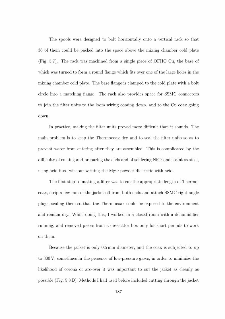
The spools were designed to bolt horizontally onto a vertical rack so that
36 of them could be packed into the space above the mixing chamber cold plate
(Fig. 5.7). The rack was machined from a single piece of OFHC Cu, the base of
which was turned to form a round flange which fits over one of the large holes in the
mixing chamber cold plate. The base flange is clamped to the cold plate with a bolt
circle into a matching flange. The rack also provides space for SSMC connectors
to join the filter units to the loom wiring coming down, and to the Cu coax going
down.
In practice, making the filter units proved more difficult than it sounds. The
main problem is to keep the Thermocoax dry and to seal the filter units so as to
prevent water from entering after they are assembled. This is complicated by the
difficulty of cutting and preparing the ends and of soldering NiCr and stainless steel,
using acid flux, without wetting the MgO powder dielectric with acid.
The first step to making a filter was to cut the appropriate length of Thermo-
coax, strip a few mm of the jacket off from both ends and attach SSMC right angle
plugs, sealing them so that the Thermocoax could be exposed to the environment
and remain dry. While doing this, I worked in a closed room with a dehumidifier
running, and removed pieces from a dessicator box only for short periods to work
on them.
Because the jacket is only 0.5 mm diameter, and the coax is subjected to up
to 300 V, sometimes in the presence of low-pressure gases, in order to minimize the
likelihood of corona or arc-over it was important to cut the jacket as cleanly as
possible (Fig. 5.8 D). Methods I had used before included cutting through the jacket
187

Figure 5.7: Thermocoax filter rack mounted on mixing chamber cold plate.
188
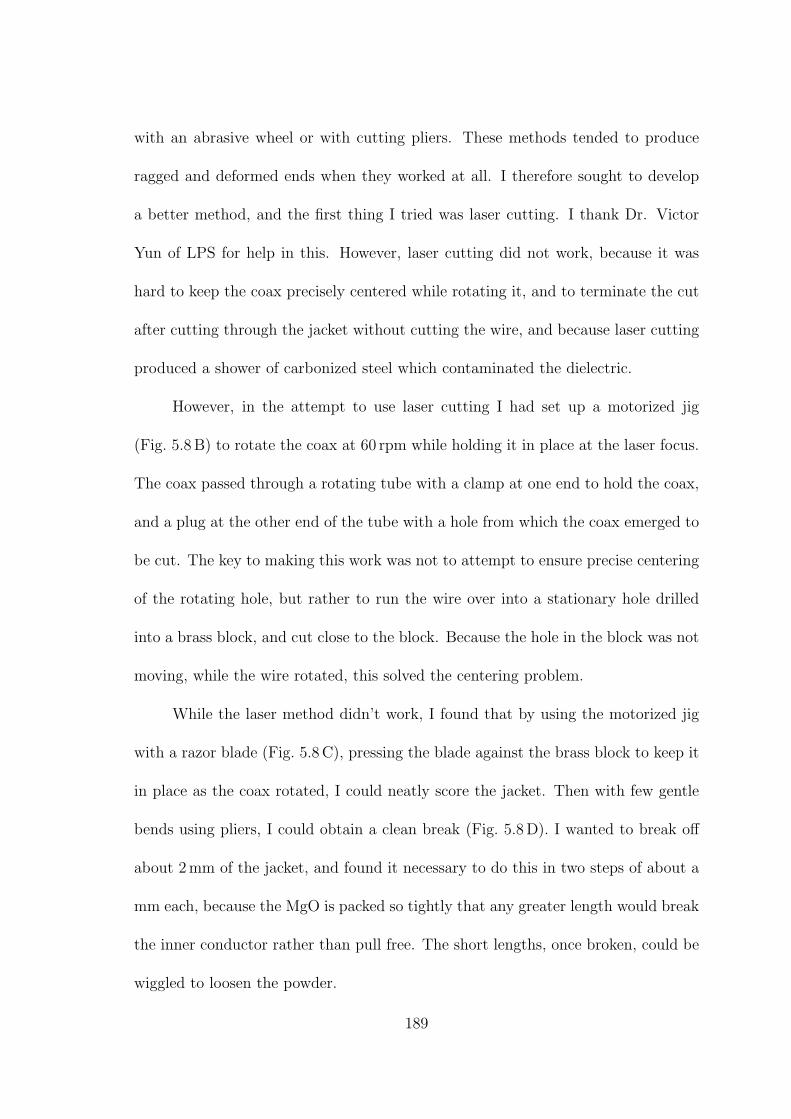
with an abrasive wheel or with cutting pliers. These methods tended to produce
ragged and deformed ends when they worked at all. I therefore sought to develop
a better method, and the first thing I tried was laser cutting. I thank Dr. Victor
Yun of LPS for help in this. However, laser cutting did not work, because it was
hard to keep the coax precisely centered while rotating it, and to terminate the cut
after cutting through the jacket without cutting the wire, and because laser cutting
produced a shower of carbonized steel which contaminated the dielectric.
However, in the attempt to use laser cutting I had set up a motorized jig
(Fig. 5.8 B) to rotate the coax at 60 rpm while holding it in place at the laser focus.
The coax passed through a rotating tube with a clamp at one end to hold the coax,
and a plug at the other end of the tube with a hole from which the coax emerged to
be cut. The key to making this work was not to attempt to ensure precise centering
of the rotating hole, but rather to run the wire over into a stationary hole drilled
into a brass block, and cut close to the block. Because the hole in the block was not
moving, while the wire rotated, this solved the centering problem.
While the laser method didn’t work, I found that by using the motorized jig
with a razor blade (Fig. 5.8 C), pressing the blade against the brass block to keep it
in place as the coax rotated, I could neatly score the jacket. Then with few gentle
bends using pliers, I could obtain a clean break (Fig. 5.8 D). I wanted to break off
about 2 mm of the jacket, and found it necessary to do this in two steps of about a
mm each, because the MgO is packed so tightly that any greater length would break
the inner conductor rather than pull free. The short lengths, once broken, could be
wiggled to loosen the powder.
189
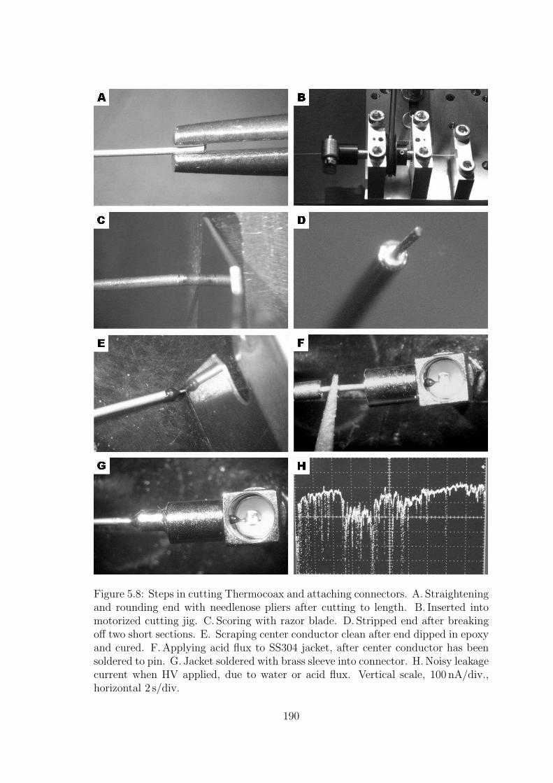
Figure 5.8: Steps in cutting Thermocoax and attaching connectors. A. Straighteningand rounding end with needlenose pliers after cutting to length. B. Inserted intomotorized cutting jig. C. Scoring with razor blade. D. Stripped end after breakingoff two short sections. E. Scraping center conductor clean after end dipped in epoxyand cured. F. Applying acid flux to SS304 jacket, after center conductor has beensoldered to pin. G. Jacket soldered with brass sleeve into connector. H. Noisy leakagecurrent when HV applied, due to water or acid flux. Vertical scale, 100 nA/div.,horizontal 2 s/div.
190
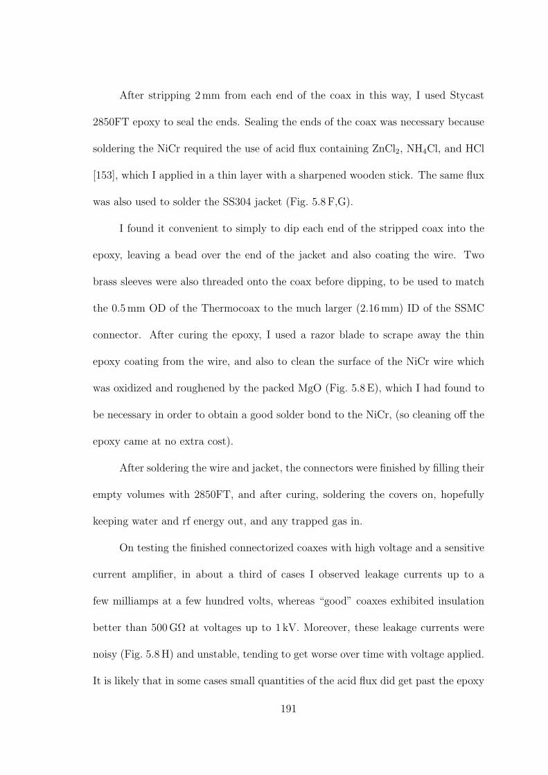
After stripping 2 mm from each end of the coax in this way, I used Stycast
2850FT epoxy to seal the ends. Sealing the ends of the coax was necessary because
soldering the NiCr required the use of acid flux containing ZnCl2, NH4Cl, and HCl
[153], which I applied in a thin layer with a sharpened wooden stick. The same flux
was also used to solder the SS304 jacket (Fig. 5.8 F,G).
I found it convenient to simply to dip each end of the stripped coax into the
epoxy, leaving a bead over the end of the jacket and also coating the wire. Two
brass sleeves were also threaded onto the coax before dipping, to be used to match
the 0.5 mm OD of the Thermocoax to the much larger (2.16 mm) ID of the SSMC
connector. After curing the epoxy, I used a razor blade to scrape away the thin
epoxy coating from the wire, and also to clean the surface of the NiCr wire which
was oxidized and roughened by the packed MgO (Fig. 5.8 E), which I had found to
be necessary in order to obtain a good solder bond to the NiCr, (so cleaning off the
epoxy came at no extra cost).
After soldering the wire and jacket, the connectors were finished by filling their
empty volumes with 2850FT, and after curing, soldering the covers on, hopefully
keeping water and rf energy out, and any trapped gas in.
On testing the finished connectorized coaxes with high voltage and a sensitive
current amplifier, in about a third of cases I observed leakage currents up to a
few milliamps at a few hundred volts, whereas “good” coaxes exhibited insulation
better than 500 GΩ at voltages up to 1 kV. Moreover, these leakage currents were
noisy (Fig. 5.8 H) and unstable, tending to get worse over time with voltage applied.
It is likely that in some cases small quantities of the acid flux did get past the epoxy
191
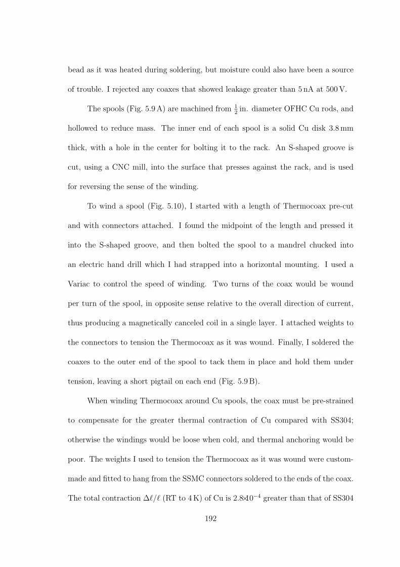
bead as it was heated during soldering, but moisture could also have been a source
of trouble. I rejected any coaxes that showed leakage greater than 5 nA at 500 V.
The spools (Fig. 5.9 A) are machined from 1
2in. diameter OFHC Cu rods, and
hollowed to reduce mass. The inner end of each spool is a solid Cu disk 3.8 mm
thick, with a hole in the center for bolting it to the rack. An S-shaped groove is
cut, using a CNC mill, into the surface that presses against the rack, and is used
for reversing the sense of the winding.
To wind a spool (Fig. 5.10), I started with a length of Thermocoax pre-cut
and with connectors attached. I found the midpoint of the length and pressed it
into the S-shaped groove, and then bolted the spool to a mandrel chucked into
an electric hand drill which I had strapped into a horizontal mounting. I used a
Variac to control the speed of winding. Two turns of the coax would be wound
per turn of the spool, in opposite sense relative to the overall direction of current,
thus producing a magnetically canceled coil in a single layer. I attached weights to
the connectors to tension the Thermocoax as it was wound. Finally, I soldered the
coaxes to the outer end of the spool to tack them in place and hold them under
tension, leaving a short pigtail on each end (Fig. 5.9 B).
When winding Thermocoax around Cu spools, the coax must be pre-strained
to compensate for the greater thermal contraction of Cu compared with SS304;
otherwise the windings would be loose when cold, and thermal anchoring would be
poor. The weights I used to tension the Thermocoax as it was wound were custom-
made and fitted to hang from the SSMC connectors soldered to the ends of the coax.
The total contraction ∆ℓ/ℓ (RT to 4 K) of Cu is 2.8×10⁻⁴ greater than that of SS304
192
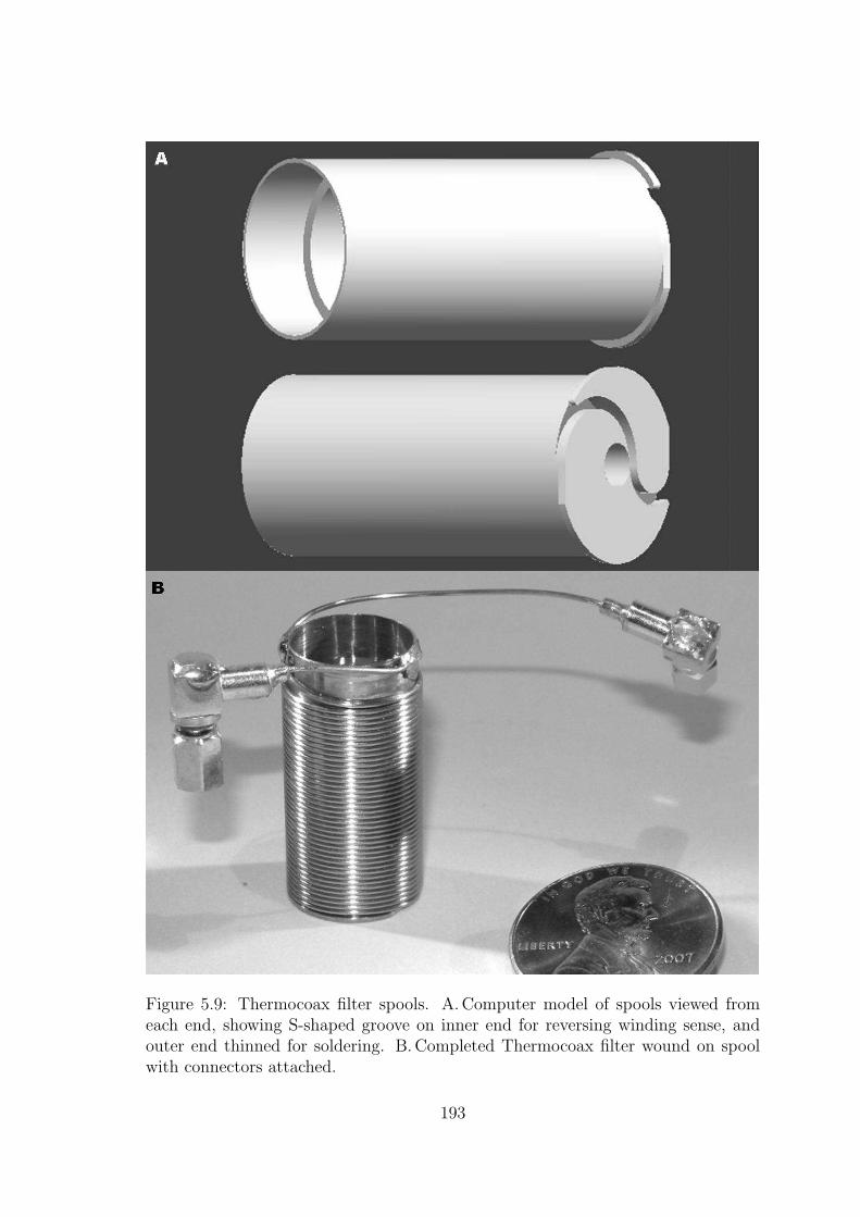
Figure 5.9: Thermocoax filter spools. A. Computer model of spools viewed fromeach end, showing S-shaped groove on inner end for reversing winding sense, andouter end thinned for soldering. B. Completed Thermocoax filter wound on spoolwith connectors attached.
193
[4], and the Young’s moduli of SS304 and NiCr are both ∼200 GPa [4, 154]. To
obtain pre-strain just greater than the predicted differential contraction would thus
require a tensile stress of 3×10−4 × 200 GPa = 60MPa. I wanted to use more, so that
the Thermocoax would make tight contact with the Cu when cold, but this purpose
could be defeated by the SS304 undergoing the austenite (face centered cubic) to
martensite (body centered cubic) phase transition, which can occur in SS304 at
temperatures around 100 K as it is cooled, and is promoted by stress [155]. To
prevent this, the stress should be kept well below 240 MPa, the 0.2% yield strength
of SS304. I compromised at 120 MPa of tensile stress, twice the minimum required
and half the yield strength. Given the 1.1×10⁻⁷m2 total cross section of the wire
and jacket, the required tension was provided by 1.3 kg weights.
5.3 Magnetically shielded sample stage for SQUID experiment
As a preliminary test of a possible principle for Josephson phase STM, we
wanted to study the behavior of an extremely asymmetric superconducting quan-
tum interference device (SQUID), consisting of two microfabricated Al-Al2O3-Al
Josephson junctions, one with a critical current I0 of ∼1µA, the other with I0 of
∼1 nA, joined in a loop of fairly large area, ∼(0.4 mm)2. Such a SQUID device was
considered as a model for a device in which the ∼1 nA junction would be formed by
a superconducting STM tip over a superconducting sample, with the ∼1µA junc-
tion added to stabilize the gauge-invariant phase difference across the tip-sample
junction, allowing changes in the loop gauge-invariant phase to be observed as the
194
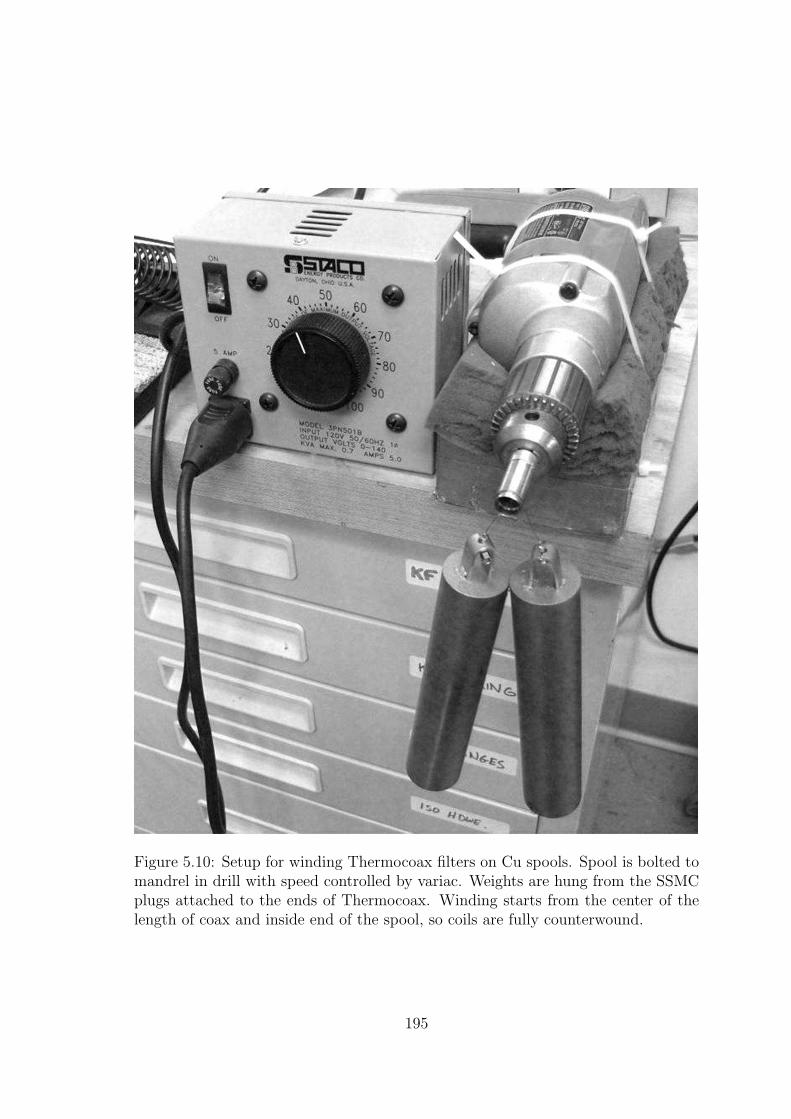
Figure 5.10: Setup for winding Thermocoax filters on Cu spools. Spool is bolted tomandrel in drill with speed controlled by variac. Weights are hung from the SSMCplugs attached to the ends of Thermocoax. Winding starts from the center of thelength of coax and inside end of the spool, so coils are fully counterwound.
195
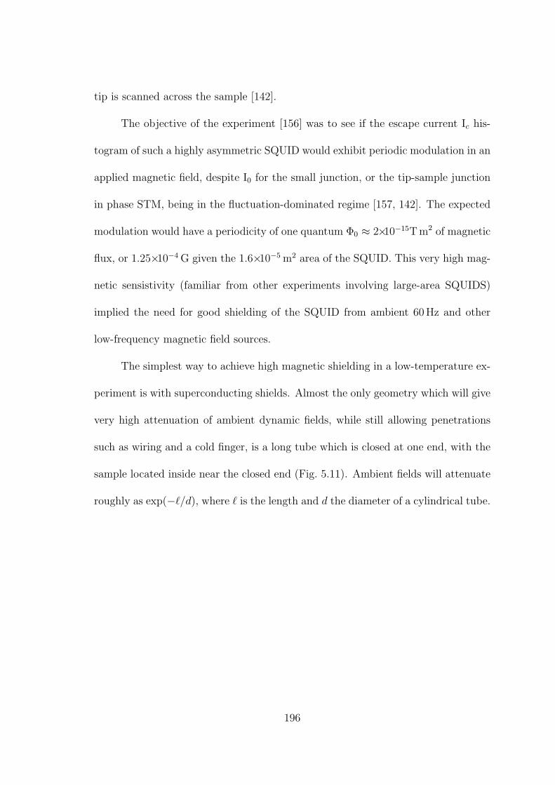
tip is scanned across the sample [142].
The objective of the experiment [156] was to see if the escape current Ic his-
togram of such a highly asymmetric SQUID would exhibit periodic modulation in an
applied magnetic field, despite I0 for the small junction, or the tip-sample junction
in phase STM, being in the fluctuation-dominated regime [157, 142]. The expected
modulation would have a periodicity of one quantum Φ0 ≈ 2×10⁻¹⁵T m2 of magnetic
flux, or 1.25×10⁻⁴ G given the 1.6×10⁻⁵ m2 area of the SQUID. This very high mag-
netic sensistivity (familiar from other experiments involving large-area SQUIDS)
implied the need for good shielding of the SQUID from ambient 60Hz and other
low-frequency magnetic field sources.
The simplest way to achieve high magnetic shielding in a low-temperature ex-
periment is with superconducting shields. Almost the only geometry which will give
very high attenuation of ambient dynamic fields, while still allowing penetrations
such as wiring and a cold finger, is a long tube which is closed at one end, with the
sample located inside near the closed end (Fig. 5.11). Ambient fields will attenuate
roughly as exp(−ℓ/d), where ℓ is the length and d the diameter of a cylindrical tube.
196
Figure 5.11: Sample stage for SQUID experiment, mounted on fridge. A. Cu cold finger with shield removed. B. Sample stagewith Al shield in place. C. Detail of sample mounting at end of cold finger. The chip is mounted directly on a header madefrom a piece of glass-epoxy board with an attached Al block, which are held onto the cold finger by 2-56 brass cap screws.Wirebonding pins are made from 00-90 brass screws, and contacted by BeCu fingers soldered to a pair of glass-epoxy boards.
197
I designed for the highest reasonably achievable attenuation, as limited by
the reach of available tooling; I used a 1 in. OD, 0.875 in. ID, 10 in. length Al
tube, giving an internal aspect ratio of about 11. As a type II superconductor,
Al below its critical temperature (∼1.1 K) will freeze in rather than exclude the
ambient dc field, but will not allow it to change, which satisfies the requirements
for the SQUID experiment. I had an Al end cap welded into one end of the tube;
although the welded area would contain many defect sites, any flux trapped in the
weld Al should be pinned at mK temperature.
The sample stage was designed to hang from the mixing chamber cold plate in
the position to be later occupied by the STM mount. A Cu cold finger runs through
from the open end to the closed end (Fig. 5.11 A). It is tightly clamped at the top
end by a block which bolts into the cold plate. The cold finger was machined from a
1 in. diameter OFHC Cu rod, most of which was first turned to 0.875 in. diameter.
Due to the low thermal conductivity of Al in the superconducting state, and
the high latent heat of the superconducting transition, I was warned that the long
tube should not be cooled from just one end. Therefore the cold finger makes contact
with the shield along its length. To achieve this, the shield was made from an Al
tube with nominal ID 0.880 in., and I used a reaming tool to cut its interior surface
to a smooth and uniform 0.875 in., so that it made a loose contact fit over the cold
finger. On cooling, the differential contraction of Al relative to Cu is 0.091%, so
that the Al tube contracts 0.0004 in. in radius relative to the Cu cold finger, enough
to guarantee pressure on the contacting surfaces (Fig. 5.11 C).
Thermocoax filters were integrated into the sample stage, occupying the upper
198
half of the cold finger (Fig. 5.11 A). Four 0.7 in. long, 0.5 in. diameter spool sections
were cut into the cold finger, and I wound 1.5 m of Thermocoax twisted pair around
each spool section, for a total of eight lines. Between each spool section a double
ring for contacting the shield was left at 0.875 in. diameter. I fed the Thermocoax
past the contacting rings through grooves cut in the length of the cold finger, and
used fine wire to tie it down.
Below the Thermocoax filters, I left a 4 in. section of the cold finger cut flat
to create a volume for additional low-frequency filters, should they be needed, or for
other experimental purposes. The cross-sectional area of the flat was equal to that
of the 0.5 in. round spool sections. The wiring in this section converted from the
Thermocoax to Cu twisted pairs which I coiled to make weak springs (Fig. 5.11 A).
Although neither these coils nor the Thermocoax filter sections were counterwound,
due to the Al shield any axial ac magnetic field should be extremely weak for the
coiled Cu twisted pairs and effectively zero for the Thermocoax coils; in addition, any
induced emf would be approximately the same for both wires of a pair. Therefore I
did not consider counterwinding to be necessary in this case.
For the SQUID experiment, the samples were mounted on removable chip
headers bolted onto the end of the cold finger, placing them in the best-shielded
location and orientation, at the far end of the shield tube, with the SQUID area
perpendicular to the axis. The chip headers conisted of machined Al blocks to
which the chips were directly attached with vacuum grease, plus wirebonding posts
mounted on a glass-epoxy skirts glued to the Al blocks (Fig. 5.11 C). I made the
skirts from pieces of electronic prototyping board pre-drilled with a 0.1 in. square
199
array of holes. To make the wirebonding posts, I threaded eight 00-90 brass screws
into the holes, soldered them to the metallization around the holes, and sanded the
screw heads flat, as a group, to create bonding pads.
I made a half-dozen copies of this chip header design. The samples were made
and mounted by Dan Sullivan, and as he preferred to solder the wires to the chip
using In, after initial failures we found that pre-tinning the brass posts with In made
this work.
Since the SQUID samples were delicate and had to be mounted and wire-
bonded on the bench, then transferred to the sample stage, it was important that
the chip headers be easily installable and that reliable electrical contact be easily
made to the bonding posts. I found scraps of BeCu finger strip intended for making
EMI gaskets, which I used to make fingers for contacting the posts. I used two more
small pieces of prototyping board, which had metallization strips running in one
direction, and soldered the BeCu fingers to the boards (underside of boards as seen
in (Fig. 5.11 C).
The boards and attached BeCu fingers were then clamped over the brass posts
with two bolts which could be loosened to release the chip headers. I varnished a
piece of heavy paper to the Cu cold finger beneath each board for insulation.
The design of the removable chip headers and the method of mounting them on
the cold finger proved reliable and easy to use in repeated trials of the experiment.
The magnetic shielding was also adequate, and we were ultimately successful in
demonstrating the observability of single flux quantum critical current modulation
in a highly asymmetric SQUID despite the unobservability of a critical current in
200
one of the two junctions [156].
5.4 Conclusions
I have described and partly assessed a set of design choices for the STM mount,
cryostat wiring and filtering, and an auxiliary sample mount for a SQUID experi-
ment. The latter was proven in a successful demonstration of the asymmetric SQUID
principle [156] intended for Josephson phase STM.
The design of the STM mount has been realized. It provides the possibility of
achieving the best shielding of the STM from ambient and thermal electromagnetic
noise. Mechanical rigidity and thermal conductance were given due consideration in
compromise the the length and mass of the (inverted) “legs”. Operational testing
is needed.
I would note that this STM mount was designed to place the STM in the
center of the high-field magnet for conventional mK-STM studies, whereas for the
proposed Josephson phase STM there will be no use for the magnet, and therefore no
need for the long pendant STM mount. Vibration of the STM, whether excited by
external sources such as ambient sound and building vibrations or internal sources
such as the 1 K pot, may turn out to be a major problem, particularly for the two-
tip STM, which is likely to be more vibration-sensitive than the simpler single-tip
STM. If this is the case, serious consideration should be given to redesigning the
STM mount either to shorten its “legs” or eliminate them entirely in favor of a more
rigid connection between the STM body and the mixing chamber cold plate.
201
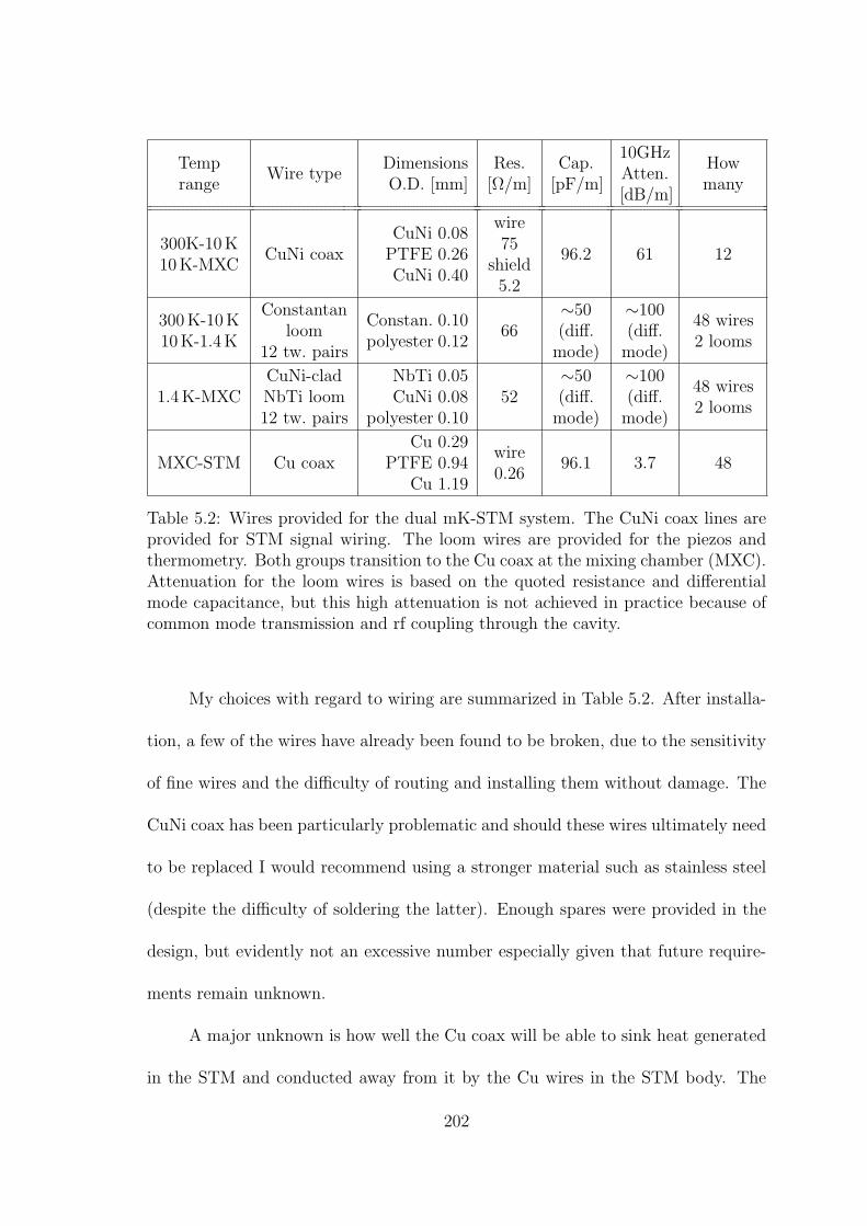
Temprange
Wire typeDimensionsO.D. [mm]
Res.[Ω/m]
Cap.[pF/m]
10GHzAtten.[dB/m]
Howmany
300K-10 K10 K-MXC
CuNi coaxCuNi 0.08
PTFE 0.26CuNi 0.40
wire75
shield5.2
96.2 61 12
300 K-10 K10 K-1.4 K
Constantanloom
12 tw. pairs
Constan. 0.10polyester 0.12
66∼50(diff.
mode)
∼100(diff.
mode)
48 wires2 looms
1.4 K-MXCCuNi-cladNbTi loom12 tw. pairs
NbTi 0.05CuNi 0.08
polyester 0.1052
∼50(diff.
mode)
∼100(diff.
mode)
48 wires2 looms
MXC-STM Cu coaxCu 0.29
PTFE 0.94Cu 1.19
wire0.26
96.1 3.7 48
Table 5.2: Wires provided for the dual mK-STM system. The CuNi coax lines areprovided for STM signal wiring. The loom wires are provided for the piezos andthermometry. Both groups transition to the Cu coax at the mixing chamber (MXC).Attenuation for the loom wires is based on the quoted resistance and differentialmode capacitance, but this high attenuation is not achieved in practice because ofcommon mode transmission and rf coupling through the cavity.
My choices with regard to wiring are summarized in Table 5.2. After installa-
tion, a few of the wires have already been found to be broken, due to the sensitivity
of fine wires and the difficulty of routing and installing them without damage. The
CuNi coax has been particularly problematic and should these wires ultimately need
to be replaced I would recommend using a stronger material such as stainless steel
(despite the difficulty of soldering the latter). Enough spares were provided in the
design, but evidently not an excessive number especially given that future require-
ments remain unknown.
A major unknown is how well the Cu coax will be able to sink heat generated
in the STM and conducted away from it by the Cu wires in the STM body. The
202
problem is not the volume thermal conductance of the PTFE dielectric, which in
the given coaxial geometry is adequate even at mK temperatures, but rather the
boundary resistance. This would be greater than the volume resistance even if the
interface were under high pressure, and obviously becomes extremely large if the
pressure goes to zero, or no contact, when the PTFE contracts at low temperature.
The latter effect is mitigated by the many bends in the Cu coax, as well as by
the clamps which are designed to partially flatten sections of the coax ensuring
maintenance of contact; however, the pressure that will remain on the interface
between the Cu jacket and the PTFE is unknown.
It is possible that the scheme of using the Cu coax as a heat sink will prove to
be inadequate, requiring a redesign to better ensure heat sinking close to the STM.
In that case, however, it is also likely that the STM body needs some redesign since
the wiring within the existing STM bodies provide only poor thermal linkage at
several connection points.
A possible improvement on the wiring choices would be to provide a number
of individually electrically shielded twisted pairs with good control of geometry and
minimization of any enclosed area where the paired wires are separated, for possible
use either as STM signal wires in a scheme like that of le Sueur et al. [144], or other
experimental needs which may arise. This would necessitate also the development
of a twisted-pair filter of some kind, but we have several options for this.
Realization of both Thermocoax and metal powder filters, in sufficiently com-
pact form to accomodate the large number of lines into the shielded STM can,
proved to be tedious and difficult, and there is considerable room for improvement
203
here, although the filters as realized will support initial experiments in mK-STM
and our efforts to develop phase STM.
Based on considerations discussed in Sec. 3.4, I would now consider microfab-
ricated distributed RC filters [106] or stripline filters using ferromagnetic aborbers
[96, 97] as alternative filter technologies. The micro-RC filters add less capacitance,
at the cost of somewhat higher resistance, for the same attenuation performance
as Thermocoax, and provide the added benefit of good thermal anchoring. The
stripline filters are compact and easy to make, and provide impedance matching
with near zero capacitance. Another possibility for the signal wires, with built-in
filtering, would be close-shielded twisted pair wiring [112, 113], but microphonic
effects might be a problem, requiring careful attention to mechanical construction
and installation.
204
Chapter 6
Conclusions and Further Work
6.1 Conclusions from the work done so far
To put an STM into a dilution refrigerator is not difficult; this was done by
Hess, et al. as early as 1989 [158], but with the result that “The microscope was
operated at 0.3±0.1 K,” and the benefits of operation at lower temperatures were not
obtained. Major problems in mK-STM include simultaneous vibration isolation and
cooling of the STM tip, sample and piezos; low-noise preamplification and electrical
filtering of the wires to prevent heating and smearing of spectra by ambient and
thermal rf voltages; thermalization of the wires and sinking of both heat conducted
down from warmer stages and heat generated by the STM head; elimination of noise
generated by the 1 K pot; and the engineering of sample and tip exchange between
RT and the mK environment.
Controlling all these problems simultaneously requires careful consideration of
many details of mK science and technology which can be contrary to intuition de-
veloped from work at room temperature or even under milder cryogenic conditions.
The heat capacities and thermal conductivities of various classes of materials, the
contributions of radiation and gas conduction to thermal transport, and the im-
portance of thermal contact resistance may all scale with different exponents of
temperature, meaning that the balance of these phenomena is qualitatively differ-
205
ent at 4 K than it is at room temperature, and again qualitatively different at mK
temperatures. Below 100 mK, radiation and gas conduction are negligible factors
(Sec. 3.3.5), thermal contact resistance is often more important than bulk thermal
resistance (Sec. 3.2.4), and residual contributions to heat capacity such as ortho-
para conversion of hydrogen and the nuclear spin states of Cu need to be considered,
as well as heat sources such as eddy currents and mechanical vibration (Sec. 3.3.6).
Success is also, inevitably, an iterative process building on knowldege gained
from earlier attempts.
Although many commercial dilution refrigerators can reach base temperatures
below 10 mK, experience has shown that when complex experimental apparatus are
built in them, with many wires in and out and several levels of structure interposing
interfaces and insulating layers between the critical element of the experiment (which
one wants to keep cold) and the mixing chamber of the fridge, it is difficult to achieve
effective temperatures below about 30 mK. For mK STMs the record is particularly
bad, with early results reporting effective temperatures, as determined e.g. by the
measurement of superconducting gap spectra, as high as 200–300mK despite much
lower temperatures measured at the mixing chamber or even at the STM sample
holder. Progress has only slowly been made towards bringing spectroscopic effective
temperatures in line with fridge temperatures.
In the present work, the installation and vibration isolation of the pumps and
plumbing appears to have been done in a satisfactory manner as judged by the fact
that low-frequency acceleration at the tabletop was increased by less than 10% as
compared with the level observed with the pumps off and no plumbing connections
206
to the table (Sec. 4.11, Table 4.1). Marginal improvement might be possible by
adding damping (e.g. cloth shrouds) to the T-bellows (Sec. 4.10), or by adding
better isolation under the 3He rotary pump (Sec. 4.8). The sandbox may have been
superfluous, but would have been more effective if incorporated into the shielded
room wall to better control vibrations of the wall (Sec. 4.9). Lining the shielded
room with sound-absorbing material will most likely be important to reduce higher-
frequency vibrations acoustically transmitted to the tabletop.
The electrical low-pass filtering described here could probably be improved but
is good enough for a first attempt to record STM images and spectra at mK tempera-
tures. Better filtering technologies have been reported in the last few years than were
known when I began this work. In particular, the use of ferromagnetic/ferrimagnetic
microwave absorbing materials is a considerable improvement over conventional
metal powder filters and should make filter fabrication far less laborious. Micro-
fabricated distributed RC filters are another compact, high-performing type which
have the added benefit of providing good heat sinking.
The wiring, as installed, should provide adequate electrical performance, and
should be adequately cooled with respect to heat conducted down from RT and
from warmer to colder stages of the fridge. However, my use of Cu-PTFE-Cu coax
as a heat sink for heat generated within the STM is dubious and may not provide
sufficient cooling. If better cooling of the STM is required, it probably will be
necessary to add specially designed heat sinks, such as metallized polyester film,
close to the tip and sample holders, or perhaps in the space just above the STM
body. In either case, some redesign of the STM body will probably be needed, either
207
to make space for heat sinking devices close to the heat sources or for better thermal
links to carry heat away from the sources to heat sinks mounted outside the STM
body.
6.2 Further work
In the immediate future, we intend to complete the installation of a dual-tip
STM in the cryostat as wired, and of supporting electronics outside, cool down and
begin testing the STM system.
Initial samples for characterization and debugging of the system may include
graphite, Au, Si, and NbSe2 or a conventional superconductor such as Nb or Al
for assessment of effective temperature and spectroscopic resolution. We are also
interested in the use of superconducting tips e.g. of Nb or Al, and we will want
to test these against both normal and superconducting samples. However, there
are many issues to be worked out regarding tip and sample preparation before this
can be done effectively. The sample preparation vacuum chambers will need to be
installed and the sample exchange mechanism will need to be operating reliably so
that samples can be cleaned or cleaved under UHV, and techniques for Nb or Al tip
preparation will need to be developed.
Ultimately we intend to use this system to study phenomena of interest in
the development of quantum computing technologies, including Si-based and super-
conducting qubit technologies. This may include the study of isolated donor states
in Si, as well as spectroscopic study of quasiparticle states in high-temperature su-
208
perconductors, exotic superconductors such as ruthenates and uranium compounds,
and the pnictides. Even where the characteristic energy scales or critical tempera-
tures for such phenomena are well above the mK range, ultralow temperatures, as
well as the use of superconducting tips, provide the best spectroscopic resolution
and aid in the discrimination of states with small energy differences. Another area
of interest for superconducting quantum computing is the study of defects in Al2O3
and other materials used as insulators in superconducting qubits. It may be useful
to study the dynamic behavior of such states at the temperatures at which qubit
experiments are normally performed.
A further goal is the development of some technique for observing the guage-
invariant phase of the superconducting order parameter in superconducting samples.
This should be possible by using a two-tip STM with superconducting tips joined
by a superconducting bridge to form a SQUID. However, this is complicated by
the fact that it is normally only possible to observe a small fluctuation-dominated
tunneling current in Josephson STM [157]. One possible solution to this problem
is the asymmetric SQUID scheme proposed by Wellstood et al [142] and validated
in our asymmetric SQUID experiment [156]. However, I would speculate that the
fluctuation-dominated Josephson tunneling will also exhibit modulation in the en-
closed gauge-invariant phase if two tips operating in this regime are configured
together as a SQUID.
209
Bibliography
[1] Robert D. McCarty. Thermodynamic Properties of Helium 4 from 2 to 1500K at Pressures to 108 Pa. Journal of Physical and Chemical Reference Data,2, 923–1041, 1973.
[2] N. H. Balshaw. Practical Cryogenics. Oxford Instruments SuperconductivityLimited, 1996.
[3] Y. H. Huang and G. B. Chen. A practical vapor pressure equation for helium-3from 0.01 K to the critical point. Cryogenics, 46, 833–839, 2006.
[4] Jack W. Ekin. Experimental Techniques for Low-Temperature Measurements:
Cryostat Design, Material Properties, and Superconductor Critical-Current
Testing. Oxford University Press, 2006.
[5] Guglielmo Ventura and Lara Risegari. The Art of Cryogenics: Low-
Temperature Experimental Techniques. Elsevier, 2008.
[6] Michael Shapiro, Vladislav Dudko, Victor Royzen, Yuri Krichevets, SamuelLekhtmakher, Victor Grozubinsky, Moshe Shapira, and Moti Brill. Charac-terization of Powder Beds by Thermal Conductivity: Effect of Gas Pressureon the Thermal Resistance of Particle Contact Points. Particle and Particle
Systems Characterization, 21, 268–275, 2004.
[7] Y. S. Touloukian, R. W. Powell, C. Y. Ho, and P. G. Klemens. Thermal
Conductivity: Nonmetallic Solids, volume 2 of Thermophysical Properties of
Matter. IFI/Plenum, 1970.
[8] Rami Ceramic Industries, Nazareth, Palestine;http://www.circonio.net/rimax.pdf (21 June 2010).
[9] James F. Shackelford and William Alexander, editors. CRC Materials Science
and Engineering Handbook, Third Edition. Chemical Rubber Company.
[10] Australia Azom.com, New South Wales. Zirconia ZrO2Grades, Mechanical, Thermal and Electrical Properties.http://www.azom.com/details.asp?ArticleID=3272 (21 June 2010).
[11] CALCE. Hardness of Materials.
[12] H. Carreon, A. Ruiz, J. Zarate, and G. Barrera. Ultrasonic Velocity Measure-ments in Alumina-Zirconia Ceramic Composite System.
[13] Structure Probe Inc. SPI Supplies Brand MgO Magnesium Ox-ide Single Crystal Substrates, Blocks, and Optical Components.http://www.2spi.com/catalog/submat/magnesium-oxide.shtml (August2010).
210
[14] E. W. Muller. Elektronenmikroskopishe Beobachtungen von Feldkathoden.Zeitschrift fur Physik, 106, 541–550, 1937.
[15] E. W. Muller. Weitere Beobachtungen mit dem Feldelektronenmikroskop.Zeitschrift fur Physik, 108, 668–680, 1938.
[16] Erwin W. Muller. Study of Atomic Structure of Metal Surfaces in the FieldIon Microscope. Journal of Applied Physics, 28(1), 1–6, January 1957.
[17] R.F. Hochman, E.W. Muller, and B. Ralph, editors. Applications of field-
ion microscopy in physical metallurgy and corrosion. Georgia Institute ofTechnology, 1969.
[18] Erwin W. Muller. Die Sichtbarmachung einzler Atome und Molekule imFeldelektronenmikroskop. Zeitschrift fur Naturforschung, 5a, 473–479, 1950.
[19] Michael K. Miller, Philippe J. Pareige, and Kaye F. Russell. Seeing and Catch-ing Atoms: ORNL’s Atom Probe Field Ion Microscope. Oak Ridge National
Laboratory Review, 28, 1995. http://www.ornl.gov/info/ornlreview/rev28-4/text/atoms.htm (July 2010).
[20] A. V. Crewe, J. Wall, and J. Langmore. Visibility of Single Atoms. Science,168(3937), 1338–1340, June 1970.
[21] R. M. Henkelman and F. P. Ottensmeyer. Visualization of Single Heavy Atomsby Dark Field Electron Microscopy. Proc Nat. Acad. Sci. USA, 68(12), 3000–3004, December 1971.
[22] L. Reimer and H. Kohl. Transmission Electron Microscopy: Physics of Image
Formation, 5th Edition. Springer, 2008.
[23] Taylor Hobson Ltd, Leicester, UK. History. http://www.taylor-hobson.com/history.html (August 2010).
[24] G. Binnig, H. Rohrer, Ch. Gerber, and E. Weibel. Surface Studies by ScanningTunneling Microscopy. Physical Review Letters, 49, 57–61, 1982.
[25] D. M. Eigler and E. K. Schweizer. Positioning single atoms with a scanningtunneling microscope. Nature, 344, 524–526, 1990.
[26] C. Julian Chen. Introduction to Scanning Tunneling Microscopy. OxfordUniversity Press, 1993.
[27] Russell Young, John Ward, and Fredric Scire. The Topografiner: An Instru-ment for Measuring Surface Microtopography. Review of Scientific Instru-
ments, 43(7), 999–1011, July 1972.
[28] G. Binnig, H. Rohrer, Ch. Gerber, and E. Weibel. Tunneling through a con-trollable vacuum gap. Applied Physics Letters, 40, 178–180, 1982.
211
[29] G. Binnig and H. Rohrer. Scanning Tunneling Microscopy. Surface Science,126, 236–244, 1983.
[30] G. Binnig, H. Rohrer, Ch. Gerber, and E. Weibel. 7 x 7 Reconstruction onSi(111) Resolved in Real Space. Physical Review Letters, 50, 120–123, 1983.
[31] J. Frohn, J. F. Wolf, K. Besocke, and M. Teske. Coarse tip distance adjust-ment and positioner for a scanning tunneling microscope. Review of Scientific
Instruments, 60, 1200–1201, 1989.
[32] G. Binnig and D. P. E. Smith. Single-tube three-dimensional scanner forscanning tunneling microscopy. Review of Scientific Instruments, 57, 1688–1689, 1986.
[33] C. Julian Chen. Electromechanical deflections of piezoelectric tubes with quar-tered electrodes. Applied Physics Letters, 60, 132–134, 1992.
[34] M. D. Kirk, T. R. Albrecht, and C. F. Quate. Low-temperature atomic forcemicroscopy. Review of Scientific Instruments, 59, 833–835, 1988.
[35] Douglas P. E. Smith and Gerd Binnig. Ultrasmall scanning tunneling micro-scope for use in a liquid-helium storage Dewar. Review of Scientific Instru-
ments, 57, 2630–2631, 1986.
[36] A. Guha, S. Kim, and A. L. de Lozanne. Novel frictionless approach mecha-nism for a scanning tunneling microscope. Review of Scientific Instruments,74, 4384–4388, 2003.
[37] K. Besocke. An easily operable scanning tunneling microscope. Surface Sci-
ence, 181, 145–153, 1987.
[38] R. R. Schulz and C. Rossel. Beetle-like scanning tunneling microscope forultrahigh vacuum and low-temperature applications. Review of Scientific In-
struments, 65, 1918–1922, 1994.
[39] Christine Meyer, Omar Squali, Heribert Lorenz, and Khaled Karrai. Slip-stickstep-scanner for scanning probe microscopy. Review of Scientific Instruments,76, 063706 (5pp.), 2005.
[40] C. Dubois, P. E. Bisson, A. A. Manuel, and Ø. Fischer. Compact design of alow temperature XY stage scanning tunneling microscope. Review of Scientific
Instruments, 77, 043712–043717, 2006.
[41] Weida Wu, Ayan Guha, Suenne Kim, and Alex de Lozanne. A Compact Dual-Tip STM Design. IEEE Transactions on Nanotechnology, 5, 77–79, 2006.
[42] Anjan K. Gupta, Rajiv Shankar Sinha, and Reetesh Kumar Singh. Compacttwo-dimensional coarse-positioner for scanning probe microscopes. Review of
Scientific Instruments, 79, 063701 (3pp.), 2008.
212
[43] S. H. Pan, 1993. World Intellectual Property Organization PatentWO 93/19494.
[44] S. H. Pan, E. W. Hudson, and J. C. Davis. 3He refrigerator based very lowtemperature scanning tunneling microscope. Review of Scientific Instruments,70, 1459–1463, 1999.
[45] Earle H. Kennard. Kinetic Theory of Gases. McGraw-Hill, 1938.
[46] Charles Kittel. Introduction to Solid State Physics. Wiley, 6th edition, 1986.
[47] Y. S. Touloukian, R. W. Powell, C. Y. Ho, and P. G. Klemens. Thermal Con-
ductivity: Metallic Elements and Alloys, volume 1 of Thermophysical Proper-
ties of Matter. IFI/Plenum, 1970.
[48] J. M. Ziman. Principles of the Theory of Solids, 2nd Ed. Cambridge UniversityPress, 1972.
[49] Frank Pobell. Matter and Methods at Low Temperatures, 2nd Ed. Springer,1996.
[50] P. G. Klemens and G. Neuer. Landolt-Bornstein New Series, Group III, Vol.
15, Metals: Electronic Transport Phenomena, Subvolume c:Thermal Conduc-
tivity of Pure Metals and Alloys, chapter Thermal conductivity of alloys, pages126–127. Springer-Verlag, 1991.
[51] K. Gloos, C. Mitschka, F. Pobell, and P. Smeibidl. Thermal conductivity ofnormal and superconducting metals. Cryogenics, 30, 14–18, 1990.
[52] L. Risegari, M. Barucci, E. Olivieri, E. Pasca, and G. Ventura. Measure-ment of the thermal conductivity of copper samples between 30 and 150 mK.Cryogenics, 44, 875–878, 2004.
[53] A. C. Anderson, W. Reese, and J.C. Wheatley. Thermal Conductivity of SomeAmorphous Dielectric Solids Below 1oK. Review of Scientific Instruments, 34,1386–1390, 1963.
[54] Dennis S. Greywall. Thermal conductivity of normal liquid 3He. Physical
Review B, 29, 4933–4945, 1984.
[55] J. R. Olson. Thermal conductivity of some common cryostat materials between0.05 and 2 K. Cryogenics, 33, 729–731, 1993.
[56] A. Kushino, M. Ohkubo, and K. Fujioka. Thermal conduction measurementof miniature coaxial cables between 0.3 and 4.5 K for the wiring of supercon-ducting detectors. Cryogenics, 45, 637–640, 2005.
[57] A. C. Anderson. Amorphous Solids: Low-Temperature Properties, chapterThermal Conductivity, pages 65–80. Springer-Verlag, 1981.
213
[58] W. Reese and J. E. Tucker. Thermal Conductivity and Specific Heat of SomePolymers between 4.5o and 1oK. Journal of Chemical Physics, 43, 105–114,1965.
[59] T. Scott and M. Giles. Dislocation Scattering in Teflon at Low Temperatures.Physical Review Letters, 29, 642–643, 1972.
[60] C. L. Tsai, H. Weinstock, and Jr. W. C. Overton. Low temperature thermalconductivity of stycast 2850FT. Cryogenics, 18, 562–563, 1978.
[61] F. Rondeaux, Ph. Bredy, and J. M. Rey. Thermal Conductiv-ity Measurements of Epoxy Systems at Low Temperature, 2001.http://irfu.cea.fr/Phocea/file.php?class=std&&file=Dpc/Publications/Archives/stcm-01-09.pdf (14 July 2010).
[62] J. H. McTaggart and G. A. Slack. Thermal conductivity of General ElectricNo. 7031 varnish. Cryogenics, 9, 384–385, 1969.
[63] A. C. Anderson and R. E. Peterson. Selection of a thermal bonding agent fortemperatures below 1 K. Cryogenics, 10, 430–433, 1970.
[64] R. B. Stephens. Low-Temperature Specific Heat and Thermal Conductivityof Noncrystalline Dielectric Solids. Physical Review B, 8, 2896–2905, 1973.
[65] W. H. Keesom and A. P. Keesom. On the Heat Conductivity of Liquid Helium.Physica, 3, 359–360, 1936.
[66] O. V. Lounasmaa. Experimental Principles and Methods Below 1K. AcademicPress, 1974.
[67] R. M. Mazo. Theoretical studies on low temperature phenomena. PhD thesis,Yale University, 1955.
[68] W. A. Little. The Transport of Heat Between Dissimilar Solids at Low Tem-peratures. Canadian Journal of Physics, 37, 334–349, 1959.
[69] R. E. Peterson and A. C. Anderson. The Kapitza Thermal Boundary Resis-tance. Journal of Low Temperature Physics, 11, 639–665, 1973.
[70] E. T. Swartz and R. O. Pohl. Thermal Boundary Resistance. Reviews of
Modern Physics, 61, 605–668, 1989.
[71] Roshdi Rashed. A Pioneer in Anaclastics: Ibn Sahl on Burning Mirrors andLenses. Isis, 81, 464–491, 1990.
[72] Lawrence E. Kinsler and Austin R. Frey. Fundamentals of Acoustics, 2nd Ed.
John Wiley & Sons, 1962.
[73] P. V. E. McClintock, D. J. Meredith, and J. K. Wigmore. Matter at Low
Temperatures. Wiley-Interscience, 1984.
214
[74] Gerald L. Pollack. Kapitza Resistance. Reviews of Modern Physics, 41, 48–81,1969.
[75] David Cheeke and Henry Ettinger. Macroscopic Calculation of the KapitzaResistance between Solids and Liquid 4He. Physical Review Letters, 37, 1625–1628, 1976.
[76] N. S. Snyder. The Kapitza Conductance of the (100) Surface of Copper. Jounal
of Low Temperature Physics, 22, 257–284, 1976.
[77] R. Berman and C. F. Mate. Thermal Contact at Low Temperatures. Nature,182, 1661–1663, 1958.
[78] Jack H. Colwell. The Performance of a Mechanical Heat Switch at Low Tem-peratures. Review of Scientific Instruments, 40, 1182–1186, 1969.
[79] I. Didschuns, A. L. Woodcraft, D. Bintley, and P. C. Hargrave. Thermalconductance measurements of bolted copper to copper joints at sub-Kelvintemperatures. Cryogenics, 44, 293–299, 2004.
[80] E. Gmelin, M. Asen-Palmer, M. Reuther, and R. Villar. Thermal boundaryresistance of mechanical contacts between solids at sub-ambient temperatures.Journal of Physics D: Applied Physics, 32, R19–R43, 1999.
[81] Angel Colin. Thermal contact resistance of different materials between 0.3 Kand 4.5 K. Cryogenics, 48, 35, 2008.
[82] Louis J. Salerno, Peter Kittel, and Alan L. Spivak. Thermal Conductanceof Pressed Metallic Contacts Augmented with Indium Foil or Apiezon-NTM
Grease at Liquid Helium Temperatures. NASA Technical Memorandum108779, National Aeronautics and Space Administration, July 1993.
[83] R. Berman. Some Experiments on Thermal Contact at Low Temperatures.Journal of Applied Physics, 27, 318–323, 1956.
[84] Y. Hariharan, M. P. Janawadkar, and T. S. Radhakrishnan. Electrical andthermal conductivity of soft solder at low temperatures. Pramana, 13, 117–125, 1979.
[85] Jr. William A. Steyert. Thermal Transport Across Superconducting SolderJoints Near 0.1oK. Review of Scientific Instruments, 38, 964–966, 1967.
[86] Guy K. White. Experimental Techniques in Low-Temperature Physics. OxfordUniversity Press, 3rd edition, 1979.
[87] Benjamin B. Dayton. Foundations of Vacuum Science and Technology, chapterKinetic Theory of Gases, pages 1–79. Wiley-Interscience, 1998.
[88] R. B. Dingle. The anomalous skin effect and the reflectivity of metals. Physica,19, 311–347, 1953.
215
[89] C. A. Bailey. Advanced Cryogenics, chapter Heat Transfer and Thermal Insu-lation, pages 133–153. Plenum Press, London, 1971.
[90] A. B. Zorin. The thermocoax cable as a microwave frequency filter for singleelectron circuits. Review of Scientific Instruments, 66, 4296–4300, 1995.
[91] John M. Martinis, Michel H. Devoret, and John Clarke. Experimental testsfor the quantum behavior of a macroscopic degree of freedom: The phasedifference across a Josephson junction. Physical Review B, 35, 4682–4696,1987.
[92] Akio Fukushima, Akira Sato, Akio Iwasa, Yasuhiro Nakamura, Takeshi Ko-matsuzaki, and Yasuhiko Sakamoto. Attenuation of Microwave Filters forSingle-Electron Tunneling Experiments. IEEE Transactions on Instrumenta-
tion and Measurement, 46, 289–293, 1997.
[93] K. Bladh, D. Gunnarsson, E. Hurfeld, S. Devi, C. Kristoffersson,B. Smalander, S. Pehrson, T. Claeson, and P. Delsing. Comparison of cryo-genic filters for use in single electronics experiments. Review of Scientific
Instruments, 74, 1323–1327, 2003.
[94] F. P. Milliken, J. R. Rozen, G. A. Keefe, and R. H. Koch. 50 Ω characteristicimpedance low-pass metal powder filters. Review of Scientific Instruments,78, 024701 (5 pp), 2007.
[95] A. Lukashenko and A. V. Ustinov. Improved powder filters for qubit measure-ments. Review of Scientific Instruments, 79, 014701 (4 pp.), 2008.
[96] D. F. Santavicca and D. E. Prober. Impedance-matched low-pass striplinefilters. Measurment Science and Technology, 19, 087001 (5 pp), 2008.
[97] D. H. Slichter, O. Naaman, and I. Siddiqi. Millikelvin thermal and electricalperformance of lossy transmission line filters. Applied Physics Letters, 94,192508 (3 pp), 2009.
[98] R. G. Chambers. The Anomalous Skin Effect. Proceedings of the Royal Society
of London A, 215, 481–497, 1952.
[99] Simon Ramo, John R. Whinnery, and Theodore Van Duzer. Fields and Waves
in Communication Electronics. John Wiley & Sons, 2nd edition, 1984.
[100] John David Jackson. Classical Electrodynamics, Third Edition. Wiley, 1998.
[101] NDT Education Resource Center, http://www.ndt-ed.org (Nov. 2010).
[102] Minicircuits, Brooklyn NY, USA; Coaxial low-pass filters,http://www.minicircuits.com/products (Nov. 2010).
[103] Moe Khalil, Laboratory for Physical Sciences, unpublished data.
216
[104] Emerson & Cuming, Inc., Billerica, MA USA.
[105] Myung-Jun Park, Jaeho Choi, and Sung-Soo Kim. Wide Bandwidth Pyrami-dal Absorbers of Granular Ferrite and Carbonyl Iron Powders. IEEE Trans-
actions on Magnetics, 36, 3272–3274, 2000.
[106] Helene le Sueur and Philippe Joyez. Microfabricated electromagnetic filters formillikelvin experiments. Review of Scientific Instruments, 77, 115102 (5 pp),2006.
[107] D. Vion, P. F. Orfila, P. Joyez, and M. H. Devoret. Miniature electrical filtersfor single electron devices. Journal of Applied Physics, 77, 2519–2524, 1995.
[108] H. Courtois, O. Buisson, J. Chaussy, and B. Pannetier. Miniature low-temperature high-frequency filters for single electronics. Review of Scientific
Instruments, 66, 3465–3468, 1995.
[109] H. le Sueur. Cryogenic AFM-STM for mesoscopic physics, volume 33 of An-
nales de Physique. Societe Francais de Physique, 2008.
[110] David M. Pozar. Microwave Engineering, 3rd Ed. John Wiley & Sons, 2005.
[111] Thermocoax, Inc., Alpharetta, GA USA.
[112] Lafe Spietz, John Teufel, and R. J. Schoelkopf. A Twisted Pair CryogenicFilter, 2006. http://arxiv.org/pdf/cond-mat/0601316 (29 June 2010).
[113] Hendrik Bluhm and Kathryn A. Moler. Dissipative cryogenic filters with zerodc resistance. Review of Scientific Instruments, 79, 014703 (6 pp), 2008.
[114] J. G. Hust. Thermal Anchoring of Wires in Cryogenic Apparatus. Review of
Scientific Instruments, 41, 622–624, 1970.
[115] SC-040/50-CN-CN Coax Co., Ltd., Kanagawa Japan. URL:http://www.coax.co.jp/english/main.html (August 2010).
[116] C. Daraio, V. F. Nesterenko, E. B. Herbold, and S. Jin. Strongly nonlinearwaves in a chain of Teflon beads. Physical Review E, 72, 016603 (9 pp), 2005.
[117] Micro-Coax, Inc., Pottstown, PA USA, http://www.micro-coax.com/ (August2010).
[118] Lakeshore Cryotronics, Inc, Westerville, OH USA. Technical Wire Specifica-tions. http://www.lakeshore.com/temp/acc/am wirets.html (20 April 2010).
[119] J. W. Gardner and A. C. Anderson. Effect of neutron irradiation on thelow-temperature specific heat and thermal conductivity of magnesium oxide.Physical Review B, 23, 1988–1991, 1981.
217
[120] Glen A. Slack. Thermal Conductivity of MgO, Al2O3, Mg Al2O4, and Fe3O4
Crystals from 3 to 300 K. Physical Review, 126, 427–441, 1962.
[121] Deane K. Smith and H. R. Leider. Low-Temperature Thermal Expansion ofLiH, MgO and CaO. Journal of Applied Crystallography, 1, 246–249, 1968.
[122] D. S. Matsumoto, Jr. C. L. Reynolds, and A. C. Anderson. Thermal boundaryresistance at metal-epoxy interfaces. Physical Review B, 16, 3303–3307, 1977.
[123] Oxford Instruments, Concord, MA.
[124] Kadel Engineering Corp., Danville IN.
[125] American Magnetics, Inc., Oak Ridge, TN.
[126] Michael Dreyer, Jonghee Lee, Hui Wang, and Barry Barker. A low temperaturescanning tunneling microscopy system for measuring Si at 4.2 K. Review of
Scientific Instruments, 81, 053703 (6 pp), 2010.
[127] TMC Model 71-473-SPL; Technical Manufacturing Corporation, PeabodyMA.
[128] ETS-Lindgren, Glendale Heights, IL.
[129] Golo Power Winch, Model 12-15 RMO, Cordem Corporation, MinneapolisMN.
[130] The cable and fittings are available from McMaster-Carr, Robbinsville, NJ.
[131] GS-11D, 4.5 Hz, 4000 Ω with 18 kΩ shunt, OYO Geospace Corp, Houston TXUSA.
[132] E. I. Rivin. Passive Vibration Isolation. ASME Press, 2003.
[133] http://www.vibrasystems.com/data/CRMP-series.pdf; retrieved 30 Dec.2009.
[134] Spectrum Control, Fairview, PA, USA, D-subminiature pi-filter type 56-715-003; http://www.spectrumcontrol.com (Nov. 2010).
[135] Standard Bellows Co., Windsor Locks, CT USA.
[136] W. P. Kirk and M. Twerdochlib. Improved method for minimizing vibrationalmotion transmitted by pumping lines. Review of Scientific Instruments, 49,765–769, 1978.
[137] Roman Movshovich. Experimental Techniques in Condensed Matter Physics
at Low Temperatures, chapter Vibration Isolation, pages 129–144. Addison-Wesley, 1998.
218
[138] P. Gorla, C. Bucci, and S. Pirro. Complete elimination of 1K Pot vibrations indilution refrigerators. Nuclear Instruments and Methods in Physics Research
A, 520, 641–643, 2004.
[139] A. Raccanelli, L. A. Reichertz, and E. Kreysa. Eliminating the vibrationalnoise in continuously filled 1 K pots. Cryogenics, 41, 763–766, 2001.
[140] Joan A. Hoffmann. Superfluid 4He: On sinφ Josephson Weak Links and
Dissipation of Third Sound. PhD thesis, University of California at Berkeley,2005.
[141] J. C. Davis. Electronic Wavefunction Imaging and Spectroscopy in Metallicand Magnetic Nanostructures by Millikelvin Scanning Tunneling Microscopy,Oct 2004. http://www.dtic.mil/cgi-bin/GetTRDoc?AD=ADA426959 (July2010).
[142] J. R. Anderson, C. J. Lobb, and F. C. Wellstood. Imaging the Gauge-InvariantPhase Difference of Superconductors at the Atomic Scale. proposal to NationalScience Foundation, 2005.
[143] H. P. Ott O. Zuger and U. Durig. Variable-temperature ultrahigh vacuumscanning tunneling microscope: Mechanical and electronic instrumentation.Review of Scientific Instruments, 63, 5634–5643, 1992.
[144] Helene le Sueur and Philippe Joyez. Room-temperature tunnel current am-plifier and experimental setup for high resolution electronic spectroscopy inmillikelvin scanning tunneling microscope experiments. Review of Scientific
Instruments, 77, 123701 (5 pp.), 2006.
[145] GVL Cryoengineering, Aachen, Germany; www.GVL-Cryoengineering.de.
[146] Michael Dreyer. personal communication.
[147] Cambridge Magnetic Refrigeration, Cambridge, UK; www.cmr-direct.com.
[148] Supercon, Inc, Shrewsbury, MA USA; http://www.supercon-wire.com (Au-gust 2010).
[149] Tomohiro Matsui, Hiroshi Kambara, and Hiroshi Fukuyama. Development ofa new ULT Scanning Tunneling Microscope at University of Tokyo. Jounal of
Low Temperature Physics, 121, 803–808, 2000.
[150] T. Matsui, H. Kambara, I. Ueda, T. Shishido, Y. Miyatake, and HiroshiFukuyama. Construction of an ultra low temperature STM with a bottomloading mechanism. Physica B, 329-333, 1653–1655, 2003.
[151] H. Kambara, T. Matsui, Y. Niimi, and Hiroshi Fukuyama. Construction ofa versatile ultralow temparature scanning tunneling microscope. Review of
Scientific Instruments, 78, 073703, 2007.
219
[152] Kennametal, Inc., Fallon, NV USA.
[153] Superior No. 75, Superior Flux & Mfg. Co, Cleveland OH, USA.
[154] Roy Beardmore, Properties of Solids, http://www.roymech.co.uk (May 2010).
[155] R. P. Reed. Materials at Low Temperatures, chapter 9, Martensitic PhaseTransitions, pages 295–341. American Society for Metals, 1983.
[156] D. F. Sullivan, S. K. Dutta, M. Dreyer, M. A. Gubrud, A. Roychowdury, J. R.Anderson, C. J. Lobb, and F. C. Wellstood. Measuring the Gauge-InvariantPhase Difference of a Sub-Micron Josephson Junction in an Asymmetric DCSQUID. to be published, 2010.
[157] O. Naaman, W. Teizer, and R. C. Dynes. Fluctuation Dominated JosephsonTunneling with a Scanning Tunneling Microscope. Physical Review Letters,87, 097004 (4 pp), 2001.
[158] H. F. Hess, R. B. Robinson, and J. V. Waszczak. Vortex-core Structure Ob-served with a Scanning Tunneling Microscope. Physical Review Letters, 64,2711–2714, 1990.
220


