
ABSTRACT
SHARMA, RAJAT. Novel Pretreatment Methods of Switchgrass for Fermentable Sugar
Generation. (Under the direction of Dr Ratna Sharma-Shivappa).
Lignocellulosic biomass has proven to be a good alternative for starch based biomass for
biofuel generation. However, due to it high liginin content, pretreatment of lignocellulosc
biomass has been studied extensively for high reducing sugar generation. Two techniques for
pretreatment of switchgrass to generate reducing sugars were tested during this study: a)
Chemical pretreatment – potassium hydroxide (KOH), b) physical pretreatment -
ultrasonication.
Chemical pretreatment was aimed at studying the potential of potassium hydroxide as a
viable alternative alkaline reagent for lignocellulosic pretreatment based on its different
reactivity patterns compared to NaOH (Raymundo-Piñero et al., 2005). Performer
switchgrass was pretreated at KOH concentrations of 0.5-2% for varying treatment times at
21, 50 and 121oC. The pretreatments resulted in delignification up to 55.4% at 2% KOH,
121oC, 1h and the highest retention of reducing sugar content at 99.26% at 0.5%, 21
oC
, 12h.
Six sets of pretreatment combinations were selected for subsequent enzymatic hydrolysis
with Cellic CTec2® for sugar generation. The pretreatment combination of 0.5% KOH, 12 h,
21oC was determined to be the most effective pretreatment combination (p <0.5 ) as it
utilized the least amount of KOH while generating 582.4 mg sugar/ g raw biomass for a
corresponding % conversion ( based on reducing sugars ) of 91.8%.
The physical pretreatment technique, ultrasonication, was aimed at exploring a refinement
technique that did not involve the addition of a chemical agent. The mechanism of
ultrasonication as a mode of irradiation on biomass particles in liquid medium is cavitation,
which involves the creation of localized high temperature and pressure zones due to
collapsing of bubbles. A Hieschler UID 1000, which generated ultrasonic sound waves up to
a maximum intensity of 20 kHz and amplitude 170 micron was used for batch sonication of
the biomass. Switchgrass was ultrasonicated at 50-100% amplitude for 5-60 min in glass and
stainless steel vessels at atmospheric pressure. Treatments in stainless steel vessels were
performed with and without temperature control. Compositional analyses including acid
insoluble lignin and reducing sugars content of all sonicated samples, structural changes in
biomass structure, and enzymatic hydrolysis for reducing sugar generation from select
ultrasonicated samples was performed. Average lignin degradation of approximately 20%
and up to 85% sugar retention across all pretreatment sets was observed. The lignin and sugar
content of pretreated samples was not significantly (p > 0.05) impacted by the treatment
parameters. Based on visual evidence of disintegration from scanning electron microscopy
images and compositional analyses pretreatment conditions, two different enzyme loadings
were selected for subsequent enzymatic hydrolysis. The combination of temp controlled, 60
min sonication at 100% amplitude gave the highest sugar conversions of 84.6 and 84.7 % for
H1 (Cellic Ctec® 2) and H2 (Dyadic Alternafuel 200L) loadings, respectively.
Novel Pretreatment Methods of Switchgrass for Fermentable Sugar generation
by
Rajat Sharma
A thesis submitted to the graduate faculty of
North Carolina State University
in partial fulfillment of the
requirements for the degree of
Master of Science
Biological & Agricultural Engineering
Raleigh, North Carolina
2012
APPROVED BY:
Dr Michael D. Boyette Dr Larry F. Skyleather
Dr Ratna Sharma-Shivappa
Chair of Advisory committee

ii
BIOGRAPHY
Rajat Sharma was born on the 2nd
of December 1985 in Gwalior, Madhya Pradesh, India. He
was born in a middle class Indian family to parents who serve in the government insurance
and banking sector in India.
He completed his higher secondary education from St. Paul’s college, morar, Gwalior and
went on to pursue an undergraduate course in biotechnology engineering from Madhav
Institute of Technology and Science, Gwalior, M.P., India with honours.
He was brought up in a joint family consisting of 12 members and had a happy and endearing
childhood, in an environment filled with Hindi music and a love for cricket. At a very young
age Rajat developed a keen analytical interest in the game of cricket and that passion still
continues as he writes blogs and debates on the current cricket scenario in the world.
He realized a penchant for singing Hindustani music during his school days and has been
trying to hone his skills, though on a non professional level. He has performed in various
charity events at NC State University and is a part of a two member band, named Jugal
brandy along with fellow State college colleague, Suman Basu who plays the guitar.
His other interests include a passion for studying religion and its impact on culture, media
and politics across the world having gained a rich experience of a multi-layered, rich
complex religious history of India. He constantly video blogs and writes on modern standings
and impacts of various religious beliefs of the world, though personally remaining an
agnostic, having spiritual leaning towards pantheism.
During his undergraduate stint as a biotechnology engineer, Rajat was keenly interested in
the concept of sustainable industrial development through the use of biomass and bioproducts

iii
and went to present a review study on the use of enzymes for industrial chemical processes,
ISTE, 2005. This led to series of planned courses and a quest for advanced knowledge of
bioprocessing which made him apply to the United States for an MS program in biological
and agricultural engineering. His admission in NC State University was one of the biggest
high points of his life and he has enjoyed a challenging and rewarding stay as a master’s of
science candidate under the guidance of his advisor Dr Ratna Sharma-Shivappa.
The keen and inspiring guidance of Dr Ratna Sharma-Shivappa helped Rajat put his goals
into perspective and gradually develop key analytical abilities to put research and data into
perspective and a structured approach to interpretation of results. Through the guidance of Dr
Sharma-Shivappa and further interest in research Rajat is aiming to attain a PhD position in
the field of bio-processing after the successful completion of his master’s degree.

iv
ACKNOWLEDGEMENTS
In this wonderful and challenging journey I would foremost like to acknowledge the
contribution of my parents, Shri Ashit Kumar Sharma & Smt Neelam Sharma. I am indebted
to them to have provided me the opportunity to attain a platform as wonderful as North
Carolina State University. My late grandfather Shri Satya Pal Solanki and my sister Akshita
Sharma along with my entire family in India who have been the backbone of my life and any
mentions of them stop short of the magnitude of their contribution.
I would like to acknowledge the most important contribution towards shaping my master’s
degree program and my research project of my graduate advisor and chair of my committee
Dr Ratna Sharma Shivappa. I would like to acknowledge and appreciate the tremendous
patience she has shown in guiding me and providing direction to my work and personal life. I
would feel no shame in admitting my lack of of personal management skills and I consider
myself extremely lucky to have had a guide like Dr Sharma, whose unending support always
brought me back on my toes whenever I saw my prospects of successfully completing my
masters program dwindling. I have had the privilege of learning an unfailing sense of focus
and self motivation from her and most importantly I have learnt a very calm sense of
professionalism from her. I hope that someday, I make her proud and exhibit some sense of
imbibing the same virtues I have admired in her. Any future successes of mine will have a
huge contribution of Dr Sharma’s guidance and her determination to help me despite my
drawbacks. I would like to thank my graduate committee members, Dr Michael Boyette and
Dr Larry Stikeleather for providing me honest and quick feedback on the progress of my
research and the trust that they have invested in me to undertake such a challenging project.

v
I would like to extend a note gratitude to my colleagues in my lab who have been through my
thick and thin and provided much needed encouragement. In order of having met them I
would acknowledge the help Anusha Devi Panneerselvam gave me to settle in the lab 270B
when I first arrived at NCSU, I would gratefully acknowledge the patience has she displayed
in teaching me the nitty-gritty’s of lab work . Dr Ziyu Wang, Sneha Athalye & Bingqing
Wang’s contribution towards making me understand the discipline of life science laboratory
procedures has had a strong impact on my attitude towards laboratory research, Ximing
Zang, for always helping me share the lab equipment and being a model of perseverance and
hard work. I would also like to thank John Long for helping me become adept at handling the
Ultrasonicator. Dr Dhana Savithri and Dr Debby Clare for helping me learn HPLC in their
lab in flex laboratories, Rachel Huie for helping me with lab equipment, whenever I needed
and managing the 270A lab wonderfully, Barry Lineberger and David Buffalo for providing
technical expertise.
The acknowledgments cannot be complete without a list of teachers and faculty members
who have taught me, worked alongside me in India and these two years at NCSU. I would
like to thank, Dr Todd Klaenhammer, Dr Jay Cheng, Dr Jason Osborne, Dr Gary Gilleskie
and Dr Balaji Rao to have taught me the graduate level courses that built the foundation of
my research. I would like to extend a special mention for Dr Rodney Huffman and Dr Gary
Roberson, whom I had the privilege of working as a teaching assistant and having had
wonderful conversations ranging from, politics and science to culture and technology. I will
always cherish the wisdom they have imparted on me. I would also like to make a special
mention of Dr Nand K Sah, ex head of department, department of biotechnology, Madhav

vi
Institute of Technology, Gwalior, M.P., India to have encouraged me to study in the US and
recommending as an applicant for a master’s of science program at the BAE department at
the program at NCSU, I have rarely met a man of such knowledge and humility, Mr K K
Bakshi and Mr Alok Sajwan for being true mentors and building confidence in me and most
importantly providing a global vision.
I would like to mention my friends who have been pillars of strength and having stood by me
in times of ill health and low self belief, back in India, Vinay Haswani, Srikant Sundaran,
Honey Ramani and Naved Khan. A special mention of thanks to Lalitendu Das for being a
friend, philosopher and guide with his dual roles as an apartment mate and lab colleague, he
has been an inspiration and will always be a pivot of guidance in the future. A special word
of thanks to my roommates; Aditya Gandhi, Abhijit Sipani and Christopher Cyril Sandeep
for being younger brothers possessing better wisdom. Last but not the least, Sonali Pandey
for being my closest friend and support, without which I would never have cleared any
obstacles.
vii
TABLE OF CONTENTS
LIST OF TABLES ......................................................................................................... x
LIST OF FIGURES………………………………………………….. ............................. xi
CHAPTER 1 LITERATURE REVIEW………………………….. ............................... 1
1.1 Introduction………………………………………..... ....................................... 3
1.2 What are biofuels ............................................................................................. 5
1.2.1 Bioalcohols ........................................................................................ 5
1.2.2 Bioethanol………………………………............ ................................ 5
1.2.3 Structure of lignocellulose .................................................................. 6
1.2.4 Switchgrass as a Lignocellulosic Resource and its Advantages
in Biofuel Production ......................................................................... 7
1.2.5 Conversion of lignocellulosic feedstocks to bioethanol ....................... 8
1.3 Pretreatment ................................................................................................... 9
1.3.1 Goals of pretreatment………………………......................................... 9
1.3.2 Physical pretreatment..... ..................................................................... 9 1.3.2.1 Mechanical Communition ................................................................... 9
1.3.2.2 Pyrolisis ......................................................................................... ...10
1.3.2.3 Steam explosion………………….................... .................................. 10
1.3.2.4 Ammonia fiber explosion .................................................................. 11
1.3.2.5 Ultrasonication .................................................................................. 12
1.3.2.6 Major components of the ultrasonicator ............................................. 15
1.3.3 Chemical pretreatment ............................................................................... 16
1.3.3.1 Acid Hydrolysis ................................................................................ 16
1.3.3.2 Alkaline Hydrolysis ........................................................................... 14
1.3.3.3 KOH pretreatement ........................................................................... 20
1.3.3.4 Ozonolysis ........................................................................................ 20
1.4 Hydrolysis ............................................................................................................... 21
1.5 Objectives................................................................................................................ 22
1.6 References ................................................................................................................ 23
CHAPTER 2 POTENTIAL OF POTASSIUM HYDROXIDE PRETREATMENT OF
SWITCHGRASS FOR FERMENTABLE SUGAR PRODUCTION ............................ 28
2.1 Abstract.......................................................................................................... 28
2.2 Introduction..................................................................................................... 29
2.3 Materials and method ...................................................................................... 32
2.3.1 Biomass ............................................................................................ 32
viii
2.3.2 Pretreatment ...................................................................................... 32
2.3.3 Hydrolysis ........................................................................................ 34
2.3.4 Analytical methods ........................................................................... 34
2.3.5 Statistical analysis ............................................................................. 35
2.4 Results and discussion .................................................................................... 36
2.4.1 Composition of switchgrass .............................................................. 36
2.4.2 Effect of pretreatment conditions ..................................................... 37
2.4.3 Solid recovery ................................................................................. 37
2.4.4 Lignin reduction................................................................................ 37
2.4.5 Reducing sugar content ..................................................................... 38
2.4.6 Selection of optimal pretreatment conditions .................................... 39
2.5 Hydrolysis .................................................................................................... 40
2.6 Conclusion ................................................................................................... 41
2.7 Acknowledgements ...................................................................................... 42
2.8 References.................................................................................................... 42
CHAPTER 3 EFFECTS OF ULTRASONICATION OF SWITCHGRASS ON
FERMENTABLE SUGAR GENERATION AND STRUCTURE ABSTRACT ............ 56
3.1 Abstract........................................................................... .................................. 56
3.2 Introduction..................................................................... .................................. 57
3.3 Materials and methods ................................................................................... 59
3.3.1 Biomass preparation .......................................................................... 60
3.3.2 Compositional analysis ..................................................................... 60
3.3.3 Scanning electron microscopy ........................................................... 61
3.3.4 Pretreatment ...................................................................................... 61
3.3.5 Enzymatic hydrolysis ........................................................................ 63
3.3.6 Statistical analysis ............................................................................. 64
3.4 Results and discussion .................................................................................... 64
3.4.1 Effect of ultrasonication on switchgrass composition ................................. 64
3.4.1.1 Solid recovery .......................................................................... 65
3.4.1.2 Acid insoluble lignin ................................................................ 65
3.4.1.3 Total reducing sugars ................................................................ 66
3.4.2 Scanning electron microscopy ........................................................... 67
3.4.3 Sugar yield after enzymatic hydrolysis .............................................. 69
3.5 Conclusions .................................................................................................... 70
3.6 Acknowledgements ......................................................................................... 71
3.7 References ...................................................................................................... 72

ix
CHAPTER 4 CONCLUSIONS AND SCOPE OF FUTURE WORK ...................... 84
REFERENCES...................................................................................... ........................... 86
APPENDICES .............................................................................................................. 87
Appendix 1 Scanning electro microscopy for chapter 3 .................................... 88
Appendix 2 Statistical analysis tables and codes for
orthogonal decomposition for Chapter2 ........................................ 98
Appendix 3 SAS code for enzymatic hydrolysis data for chapter 2 .................. 131
Appendix 4 SAS code for compositional analysis for variables AIL
and sugars for chapter 3 .............................................................. 135
Appendix 5 SAS code for enzymatic hydrolysis data for chapter 3 ................... 148
x
LIST OF TABLES
Table 2.1 Conditions selected for KOH pretreatment ................................................ 48
Table 2.2 Chemical composition of performer switchgrass ....................................... 49
Table 2.3 Solid recoveries after KOH pretreatment ................................................... 50
Table 2.4 Sugar yields and % conversion for washed samples with 0% and
30% enzyme loading ................................................................................. 51
Table 2.5 Sugar yields and % conversion for dilute washed samples with 0%
and 30% enzyme loading........................................................................... 52
Table 2.6 Orthogonal decomposition of sugars variable ........................................... 53
Table 3.1 Treatment parameters investigated during ultrasonication ........................ 56
Table 3.2 Solid recoveries of ultrasonicated samples................................................ 76
Table 3.3 Sugar yields and % conversion for samples with Novozyme
Cellic® Ctec2 loadings & 0% loadings .................................................... 77
Table 3.4 Sugar loadings and % conversion for samples with Dyadic
Alternafuel 200L loadings ........................................................................ 78
xi
LIST OF FIGURES
Chapter 1
Figure 1 The photographic image of the ultrasonic instrument and
its basic embodiment .......................................................................... 16
Chapter 2
Figure 1 Percent reducing sugars in the three fixed temperature
sets, 21oC, 50
oC, 121
oC ..................................................................... 54
Figure 2 Percent Acid soluble lignin in the three fixed temperature
sets, 21oC, 50
oC, 121
oC .................................................................... 55
Chapter 3
Figure 1 Temperature and power dissipation profile during
ultrasonication of switchgrass in glass reaction
vessel ............................................................................................... 80
Figure 2 SEM images of untreated and pretreated
switchgrass 100X, 250X, 500X, magnification ................................. 81
Figure 3 Percent acid insoluble lignin content of ultrasonicated
switchgrass sample ............................................................................ 82
Figure 4 Percent reducing sugars content of ultrasonicated
switchgrass sample ............................................................................ 83

1
CHAPTER 1
Literature review
1.1 Introduction
The imminent energy crisis has led to a new found interest in exploration and development of
renewable sources of energy that are clean, efficient and safe for the environment. One such
highly acknowledged realm of cleaner fuels is bio-fuel. Bio-fuels are an inexhaustible source
of energy that offers a competent alternative to fossil fuels.
The choice of feedstock is central to the controversy surrounding bio-fuels today,
with current technologies associated with the use of food as fuel and large-scale changes in
land use. For bio-fuels to have any meaningful impact on energy, biomass feedstock must be
widely available at low cost and without negative environmental impact. Lignocelluloses -
the non-food component of plants fit this description (Mousdale, 2008). Switchgrass offers a
potential lignocellulosic alternative as it obviates the problem of food security, being a non-
edible plant source. It is available abundantly and unlike fossil fuels, which release more and
more of the CO2, energy crops like switchgrass "recycle" CO2 with each year's cycle of
growth and use and are thereby emerging as a sustainable development model (Keshwani and
Cheng, 2009).
Lignocelluloses have 3 main components: lignin, cellulose and hemicellulose. Pretreatment
of lignocelluloses is done to break down the lignin structure and disrupt the crystalline
structure of cellulose, so that enzymes can easily access and hydrolyze the cellulose for
production of fermentable sugars. A variety of pretreatments have been investigated by
several researchers, with the most common being physical and chemical pretreatments.
2
Physical pretreatments include mechanical communition, pyrolyisis, steam explosion, and
ammonia fiber explosion. These methods are energy intensive and therefore lack overall
efficiency and are not environmentally viable (Galbe and Zacchi, 2007, Kilzer and Broido,
1965).
Chemical pretreatments involve reagents such as acid and alkali. These techniques involve
treating biomass with chemicals that degrade the lignin by oxidation or hydrolysis of the
bonds in the lignocellulosic feedstock. The limitations of these techniques are production of
undesirable toxic substances that effect biofuel yield and cost effectiveness due to use of
costly non-renewable reagents (Quesada et al., 1999; Sun and Cheng, 2000).
In this review we analyze two novel pretreatment techniques, which hitherto have been
relatively unexplored for the specific need of pretreatment of lignocelluloses. The first
technique involves pretreatment of switchgrass with dilute potassium hydroxide (KOH).
KOH is a relatively unexplored chemical treatment method for lignocelluloses, primarily
because of its higher cost of purchase compared to NaOH. We opted for KOH on the basis of
studies evaluating its effect on the structure of carbon nano fibres, which suggested that KOH
degrades ordered structures in a more effective manner than NaOH (Raymundo-Piñero et al,
2005). The choice of an alkali pretreatment was also made due to higher retention of
reducing sugars in the pretreated solids (Xu et al., 2010).
The other novel technique we studied is a refined physical pretreatment process -
ultrasonication. Ultrasonication (or sonication) uses ultra high frequency sound waves to alter
the molecular structure of biomass. It is commonly applied in biological processes for
disruption of cell membranes and release cellular enzymes, also known as sonoporation

3
(Zhou et al 2008). This method was chosen for our study as it offers simple solutions to the
problems associated with conventional chemical pretreatment methods. The process uses
water as the primary reagent which is relatively more abundant compared to other reagents.
As there are no chemical reactions involved during the process there is minimal chance of
production of toxic wastes. Below we analyze results from other works/researchers using
ultrasonication (plant treatment, microbial decontamination, organic matter) and propose a
process for ultrasonic pretreatment of lignocellulose.
1.2 What are biofuels?
Biofuels are fuels that derive their energy from solid, liquid and gaseous biomass sources that
fix carbon biologically. These biomass sources are renewable plant and animal organic
materials. The most common biomass sources for fuel production being perennial grasses,
corn, algae, waste oil (Demiribas, 2009). Most contemporary fuels are biological in nature
but what sets biofuels apart is their minimal impact on the accumulation of total carbon
dioxide in the atmosphere (Demiribas, 2009). The aspect that sets biofuels apart from fossil
fuels is the sheer time scale of their development compared to fossil fuels, which have taken
thousands of years for their formation (Shrestha and Paudel, 2008). Another beneficial aspect
of biofuels is their net negative contribution to carbon emissions after burning, thus being
termed “CO2 neutral”.
Parameters that determine the viability of any biofuel including bioalcohols, biodiesel,
bioethers, biogas, syngas and solid biofuels are governed by the availability of feedstock and
4
how efficiently its energy content can be utilized (Shrestha and Paudel, 2008). The
chronological analysis of biofuel development is an interesting exploration of the sources of
biomass utilized (feedstock) and the methods utilized for their conversion. First generation
biofuels can be characterized as fuels produced from sources such as sugar, starch, and
vegetable oils or animal fats to produce fuels like bioethanol and biodiesel. The use of such
feedstock sources, especially starch, for energy production has however led to a steep rise in
food prices as most of these sources such as wheat, corn and sugarcane are major food
industry inputs and have raised apprehensions in the land usage for their production. Also,
the agricultural inputs for production of starch-based feedstocks are very high thus making
them economically unviable and the fuel generation through biological sources more
expensive than conventional sources (Keshwani and Cheng, 2009).
Biofuels derived from conventionally used starch based food sources such as corn, wheat
and sugarcane were categorized as first generation biofuels.Biofuels derived from cellulose
rich sources that are non-edible and have a greater regeneration capability are classified as
second-generation biofuels( European biofuels, 2011).This category mainly includes
resources such as corn stover, switchgrass, miscanthus, woodchips, and the byproducts of
lawn and tree maintenance which are broadly termed as lignocelluloses.
Lignocelluloses like switchgrass are perennial vegetations that have evolved over many years
of harsh sunlight and heat which have led them to adapt to harsher conditions and use the
available ground water more efficiently (Keshwani and Cheng, 2009). A disadvantage of
lignocellulosic material as compared to starch based sources is difficulty in hydrolysis.
Starch based sources such as corn can be easily hydrolyzed by enzymes or chemical reagents
5
to generate sugars for fermentation whereas due to the lignin protected carbohydrate
framework, lignocellulosic sources need to be pretreated for saccharification to be effective.
The shortcoming of lignocellulosics is however far outweighed by their benefits as they
provide environmental friendly feedstocks that would require innovative processing
technology to generate fuel that competes commercially with conventional sources to emerge
as the foundation for energy security and environment protection.
1.2.1Bioalcohols
Alcohols obtained from biological sources are known as bio-alcohols. Bio-alcohols are fast
emerging as effective alternatives to fossil fuel. Some of the advantages include high octane
numbers and comparable energy densities of bioalcohols like butanol to those of fossil fuels.
Aliphatic alcohols, being able to be synthesized biologically provide cleaner and greener
alternative to fossil fuels. (Chen et al., 2007)
1.2.2Bioethanol
“The principle fuel used as a petrol substitute for road transport vehicles is bioethanol.
Bioethanol is mainly produced by the sugar fermentation process, although it can also be
manufactured by the chemical process of reacting ethylene with steam” (what is bioethanol,
2012).It is a high-octane fuel and has replaced lead as an octane enhancer in petrol. It is a
clear, colorless, clean burning liquid fuel, which is biodegradable and does not pollute the
environment after burning (Grous et al., 1986). Bioethanol has emerged as a successful
model since ethanol-gasoline blends (E10 with 10% ethanol and 90% petrol) are being
6
commercially utilized in countries such as the United States. Sugarcane and corn are
currently the primary feedstocks for commercial bioethanol production in Brazil and US,
respectively. As mentioned previously, the drawbacks of such feedstocks have led to a surge
in research and development of techniques, methods and materials to enhance quality of
blends and reduce cost of production (Grous et al., 1986) with a significant effort being
directed towards lignocellulose conversion.
1.2.3 Structure of Lignocellulose
Lignocelluloses consist of three main components: Cellulose, Hemicellulose and Lignin.
Cellulose and hemicellulose are polymers of monosaccharides joined together by glycosidic
linkages whereas lignin is an aromatic polymer synthesized from phenylpropanoid
precursors. Cellulose makes up 45% of the biomass and it is composed of D-glucose
subunits joined together by -1,4, glycosidic linkage, which form long elemental fibrils that
are linked together by hydrogen bonds and Vander Val’s forces. Hemicelluloses and lignin
cover the microfibrils that are made by elemental fibrils. Microfibrils constitute the cellulose
fiber, which is present primarily in a crystalline form and sometimes in an amorphous form
that is relatively easily hydrolyzed (Kuhad et al., 1997). Hemicellulose is the second major
component of lignocellulose and forms about 25-30% of total dry wood weight. It consists of
all the D- pentose sugars (D-xylose, D-mannose, D-galactose, D-glucose, D-arabinose) with
D-xylose present in the largest amoint. It occasionally consists of some L-sugars as well with
small amounts of glucornic and mannuronic acids. Sugars are linked together by β-1, 4- and
occasionally β-1, 3-glycosidic bonds. Hemicellulose is more easily hydrolysed as compared
7
to celluose as it consists of branched chain of mono saccharides that often contains acetyl
groups, like hetroxylan. These do not form aggregates even when they are co-crystallized
with cellulose (Kuhad et al., 1997)
Lignin is the third major component of lignocellulose and it is the most abundant polymer
found in nature. It is found in the cell wall of plants and provides the plant with structural
support, impermeability, and resistance against microbial attack and oxidative stress. It is an
amorphous heteropolymer, insoluble in water and optically inactive consisting of Phenyl
propane subunits linked randomly thorough various types of linkages. The synthesis of
lignin constitutes the peroxidase-mediated dehydrogenation of three propionic alcohols that
leads to free radical generation. The three propionic alcohols being: guaiacyl (propanol),
coumaryl alcohol (p-hydroxyphenylpropanol), and sinapyl alcohol (syringylpropanol). The
polymerization of lignin is characterized by hetrogneous C-C and aryl-ether linkages forming
monomeric units of aryl-glycerol β aryl ether (Sánchez et al., 2009).
1.2.4 Switchgrass as a lignocellulosic resource and its advantages in biofuel production.
Switchgrass is a promising feedstock for biofuels production due to its high productivity, and
need for relatively low agricultural inputs. It is an excellent renewable source that has
multifarious environmental benefits such as, carbon sequestration, nutrient recovery from
runoff, soil remediation and provision of habitats for grassland birds. Switchgrass, on
average, consists of 45% cellulose and 35.1% hemicelluloses, making it rich in reducing
sugars. Pretreatment of switchgrass is however required to improve the yields of fermentable
sugars, as switchgrass being lignocellulosic contains a relatively high average lignin content
8
of 19% (Wiselogel et al., 1996). Based on the type of pretreatment, glucose conversion yields
from switchgrass ranged from 70% to 90% and xylose yields ranged from 70% to 100% after
hydrolysis. Following pretreatment and hydrolysis, ethanol yields in the range of 72% to
92% of the theoretical maximum have been reported (Wood and Saddler, 1988; Chum et
al.1988; Wyman et al.; 1992).
The characteristics that make switchgrass a viable biofuel feedstock option are its ability to
convert a large amount of solar energy into cellulose, which is the target molecule for
bioethanol production. It also has excellent water usage capacity as its roots dig deep into the
soil and extract ground water (Keshwani and Cheng, 2009). Switchgrass’ has the ability to
add organic matter by expanding deep into the soil and its complex underground network of
stems and roots help it to retain the soil content on the cultivated land and obviate a major
environmental concern of soil erosion and runoff. Besides helping slow runoff and anchor
soil, switchgrass can also filter runoff from fields planted with traditional row crops. Buffer
strips of switchgrass, planted along stream banks and around wetlands, could remove soil
particles, pesticides, and fertilizer residues from surface water before it reaches groundwater
or streams and could also provide energy.
1.2.5 Conversion of lignocellulosic feedstocks to bioethanol
Lignocellulosic feedstocks such as switchgrass with their high reducing sugar content have
emerged as effective bio-fuel generation sources. The basic scheme of fuel generation from
lignocellulosic feedstocks involves the following steps: a) harvest and storage b)
pretreatment c) hydrolysis and d) fermentation. Lignocellulosic sources such as switchgrass
9
requir a process of pretreatment which is aimed at making the biomass conducive for
enzymatic activity. The pretreatment step is followed by enzymatic hydrolysis and the sugars
generated from hydrolysis are then fermented to biofuels.
1.3 Pretreatment
1.3.1 Goal of pretreatment
The goals of any lignocellulose pretreatment are to breakdown lignin and/or hemicellulose or
the scaffolding of cellulose microfibrils and de-crystallize it to increase porosity of the
lignocellulosic material (Kumar et al., 2009). An effective preatment strategy must meet the
following requirements: (1) retain the carbohydrate content (2) minimize production of by-
products that affect ethanol yield, (3) improve generation of sugars after enzymatic
hydrolysis, and (4) be cost-effective (Kumar et al., 2009). A variety of pretreatment methods
have been investigated on various feedstocks.
1.3.2 Physical pretreatment
It is a technique that involves application of specific physical and mechanical stress for
disrupting the lignocellulosic structure. The various types of commonly used methods are as
follows:
1.3.2.1 Mechanical communition
Communition of lignocelluosic particles is done to achieve decrystallization of cellulose.
During this process, size of the particles is brought down to 0−30 mm after chipping and
10
0.2−2 mm after milling or grinding (Kumar et al., 2009).It has been proposed that if the final
particle size is held in the range of 3−6 mm, the energy input for comminution could be kept
below 30 kWh per ton of biomass. The energy input required for the process was however
found to be higher than the theoretical energy content available in the biomass in most cases
(Cadoche and Lopez, 1989) Irradiation of cellulose by γ-rays, which leads to cleavage of β-1,
4-glycosidic bonds and gives a larger surface area and a lower crystallinity, has also been
tested (Takacs et al., 2000). This method was deemed to be extremely cost ineffective (Galbe
and Zacchi, 2007).
1.3.2.2 Pyrolysis
Pyrolysis of biomass leads to decomposition of cellulose to gaseous products and residual
char when it is treated at temperatures greater than 300 °C (Mousdale, 2008; Keshwani and
Cheng, 2009). At lower temperatures, decomposition is much slower, and the products
formed are less volatile (Kilzer and Broido, 1965). Fan et al.(1987) reported that mild acid
hydrolysis (1 N H2SO4, 97 °C, 2.5 h) of the products from pyrolysis pretreatment resulted in
80−85% conversion of cellulose to reducing sugars with more than 50% glucose. The process
has been shown to be cost ineffective.
1.3.2.3 Steam explosion
Sudden high pressure and low-pressure steam currents bring about explosive decompression
of biomass. Steam explosion is typically initiated at a temperature of 160−260 °C
(corresponding pressure, 0.69−4.83 MPa) for several seconds to a few minutes before the
11
material is exposed to atmospheric pressure (McMillan, 1994). This process causes
hemicellulose degradation and lignin transformation due to high temperature (Sun and
Cheng, 2002). Removal of hemicelluloses from the microfibrils is believed to expose the
cellulose surface and increase enzyme accessibility to the cellulose microfibrils (Grou et al.,
1986).Rapid flashing to atmospheric pressure and turbulent flow of the material cause
fragmentation of the material, thereby increasing the accessible surface area (Li et al., 2007).
Steam explosion coupled with a catalyst is the closest to commercialization as it enjoys the
benefit of being cost and energy effective (Holtzapple et al., 1989). The limitations of this
method include the destruction of a part of the xylan fraction, incomplete disruption of the
lignin−carbohydrate matrix, and generation of compounds that might be inhibitory to
microorganisms used in downstream processes (Mackie et al., 1985).
1.3.2.4 Ammonia fiber explosion
During the ammonia fiber explosion process biomass is exposed to liquid ammonia at high
temperature and pressure and then the pressure is suddenly released. In a typical AFEX
process the dosage of liquid ammonia is 1−2 kg of ammonia/kg of dry biomass, the
temperature is 90 °C, and the residence time is 30 min (Mackie et al., 1985). AFEX has
particularly proved effective for herbaceous materials and crops. The various lignocellulosic
materials pretreated effectively by AFEX are alfalfa, wheat straw, and wheat chaff (Alizadeh
et al., 2005). During AFEX pretreatment only a small percentage of solid material is
solubilized and no hemicellulose and lignin are removed. Hemicellulose is broken down into
oligomeric sugars and deacetylated. The structure of the material is changed in the process

12
and the water holding capacity and digestibility is increased (Gollapalli et al., 2002). Over
90% hydrolysis of cellulose and hemicellulose was obtained after AFEX pretreatment of
bermudagrass (approximately 5% lignin) and bagasse (15% lignin) (Galbe and Zacchi,
2007).
1.3.2.5 Ultrasonication
Ultrasound vibrations are disturbances caused by sound waves at frequencies above the
audible range of humans at frequencies above 20 kHz (Feng et al., 20011). The acoustics
from an ultrasound irradiated system in an ultrasonic span in liquids have been shown to
effect particles in the range of 0.15mm to 100mm. There is a non linear effect of the acoustic
phenomena which depends on cavitation, which is defined as the growth and implosive
collapse of bubbles in a liquid irradiated by ultrasound. The creation of positive and negative
compression zones in the liquid by sound waves leads to the rise and recompression of
bubbles formed by the solute, solvent vapour and previously dissolved gases (Suslick et al.,
1991, 1994).
Asymmetrical collapse of the bubble leads to a jet of liquid directed at the surface (Suslick et
al., 1991, 1994). Tip jet velocities which, are generated have been measured to be greater
than 100 ms-1
. The impingement of these jets can create localized erosion (and even melting),
surface pitting, and ultrasonic cleaning. A second contribution to erosion created by
cavitation involves the impact of shock waves generated by cavitational collapse. The
magnitude of such shock waves is thought to be as high as 104
bar, which can easily produce
plastic deformation of malleable metals (Preece and Hannson, 1981).

13
Ultrasonication is a relatively less explored physical refinement pretreatment technique for
biomass. It is a method that involves the treatment of biomass through ultrasonic waves in a
liquid medium. The principle behind such a technique is the transmission of waves leading to
growth and implosive collapse of bubbles in a liquid which further leads to cavity hot spots at
temperatures of roughly 5300 K, pressures of about 1720 bar, and heating and cooling rates
above 109 K/s (Suslick et al., 1991, 1994). Recent studies on the effect of ultrasonic
irradiation of biomass have shown removal of the cellulosic fibers from the lignocellulosic
framework and release of lignin and hemicellulose from biomass particles (Zhang et al.,
2007; Xia et al.; 2004, Gronroos et al., 2004).
Zhang et al. (2007) while working on developing cellulose fibers for use as support in
composites showed that cellulose nano fibres could be extracted from lignocellulose by the
application of high intensity ultrasonication. They showed that cellulose could be treated
with ultra high frequency sound waves to produce small fibrils at nano and micro scales.
They proposed that hydrodynamic forces of ultrasound produce very strong oscillating
mechanical power, which may lead to the separation of cellulose microfibrils from the
cellulose fibre. This work indicates critically that ultrasound acoustic waves do impact the
complex lignocellulosic matrix and there is scope for more refined work in the area (Zhang et
al., 2007).
Sun et al. (2004) investigated the extractability of the hemicelluloses from bagasse obtained
by ultrasound-assisted extraction and found that ultrasonic treatment and sequential
extractions with alkali and alkaline peroxide under the conditions given led to a release of
over 90% of the original hemicelluloses and lignin. They went on to observe that
14
ultrasonication attacked the integrity of cell walls, cleaved the ether linkages between lignin
and hemicelluloses, and increased accessibility and extractability of the hemicelluloses. The
hemicellulosic fractions obtained after ultrasonic extracxtion contained relatively low
amounts of associated lignins, ranging between 0.41% and 7.36%, which was lower than
those of the corresponding hemicellulosic preparations obtained without ultrasound. The low
content of chemically linked lignin in hemicelluloses showed that the α-benzyl ether linkages
between lignin and hemicelluloses in the cell walls of bagasse were substantially cleaved
during ultrasonic irradiation (Sun et al., 2004).
Mao et al. (2007) in their work on influence of ultrasonication on anaerobic bioconversion of
sludge showed that hydrolysis rates of biomass increased considerably by pretreatment with
ultrasonication (Mao et al., 2007). Particle disruption was effected by low-frequency
ultrasound treatment, which was shown evident by a significant reduction in bioparticle size,
from 47.5 to 18.5 µm, and more than 160% increase in soluble substances. First-order
hydrolysis rates increased from 0.0384 on day 21 in the control digester to 0.0456, 0.0576,
and 0.0672 W/mL on day 21 in the digesters fed with sludge sonicated at densities of 0.18,
0.33, and 0.52 W/mL, respectively (Mao et al., 2007 ).
Wong et al. (2009) in their work on bacterial and plant cellulose modification using
ultrasound irradiation showed that depolymerization of plant (PC) and bacterial (BC)
celluloses could be achieved by employing suitable ultrasonication settings intensities.
During this study they observed a decrease in the average molecular weight of the plant
samples due to the scission of β-d-(1 → 4) glycosidic linkages after being pretreated with
ultrasonication (Wong et al., 2009).
15
They also went on to observe that a reduction in the polydispersity index (PI), which is an
indication of the segmental size distribution of a particular polymer defined as the ratio of
weight to number average molecular weight had decreased. It was thus inferred meant that
prolonged sonication yielded chain segments that could not be further degraded, an outcome
which tended to create homogeneous systems with a relatively narrow molecular weight
(Wong et al., 2009).
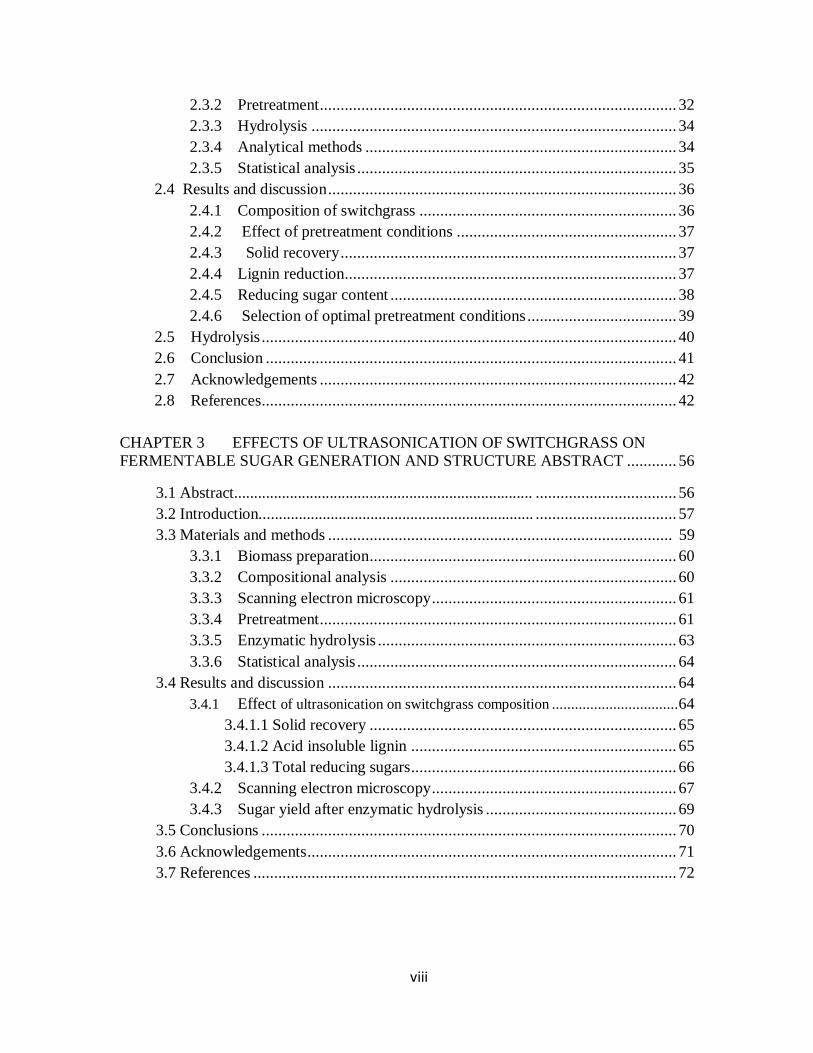
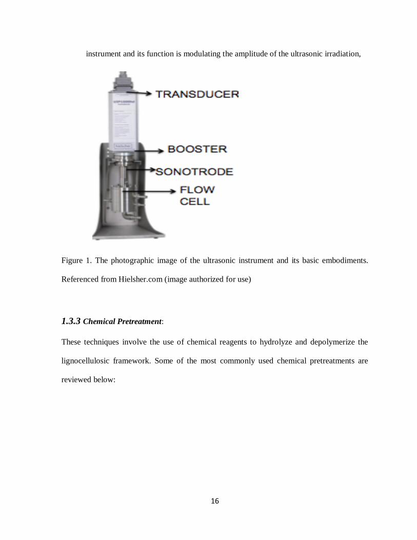
1.3.2.6 Major Components of an ultrasonicator
An ultrasonicator consists of the following parts:
Transducer: This part of the instrument converts the electrical energy from the power
source and converts it into mechanical oscillations of the range of 20KHz, which are
in the ultrasonic vibration range. It is usually made of a metallic material capable of
generating heavy oscillations.
Booster: This is a mechanical embodiment, which is responsible for increasing the
amplitude of the waves that are applied on the liquid medium.
Sonotrode: This tool which is usually made up of Tungsten is the tool that transfers
the oscillations on the medium and remains in physical contact with the medium
Continuous Flow Cell: This part contains the medium that is pretreated and usually is
made of inert material that could withstand moisture and heavy pressure and
temperature changes.
Amplitude Control Unit (not in picture): This unit is a separate entity connected to the
16
instrument and its function is modulating the amplitude of the ultrasonic irradiation,
Figure 1. The photographic image of the ultrasonic instrument and its basic embodiments.
Referenced from Hielsher.com (image authorized for use)
1.3.3 Chemical Pretreatment:
These techniques involve the use of chemical reagents to hydrolyze and depolymerize the
lignocellulosic framework. Some of the most commonly used chemical pretreatments are
reviewed below:
17
1.3.3.1 Acid Hydrolysis
In this process, dilute acid is mixed with biomass to hydrolyze hemicellulose to xylose and
other sugars. Further breakage of xylose into furfural can also occur at high temperatures
(Mosier et al., 2005). This leads to an increase in the reaction rates, which improves the
cellulose hydrolysis (Esteghlalian et al., 1997). Dilute acid effectively removes and recovers
most of the hemicellulose as dissolved sugars, and glucose yields from cellulose increase
with hemicellulose removal to almost 100% following complete hemicellulose hydrolysis.
Hemicellulose is removed when sulfuric acid H2SO4 is added and this enhances digestibility
of cellulose in the residual solids (Mosier et al., 2005). High temperature has been observed
to improve acid hydrolysis and hemicelluose breakdown (Hinman et al., 1992). As xylan
accounts for one-third of the total lignocellulose carbohydrate content, high xylan to xylose
conversion is desirable to pretreatments as has been observed in dilute acid pretreatments
(Hinman et al., 1992). Two types of dilute-acid pretreatment processes are typically used: a
high-temperature (T > 160 oC), continuous-flow process for low solid loadings (weight of
substrate/weight of reaction mixture) 5-10%) (Brennan et al. 1986, Converse et al., 1989) and
a low-temperature (T < 160oC), batch process for high solid loadings (10-40%) (Esteghlalian
et al., 1997). The most widely used and tested approaches are based on dilute sulfuric acid.
However, nitric acid (Brink, 1993), hydrochloric acid (Israilides et al. 1978, Goldstein et al.,
1983), and phosphoric acid (Israilides et al., 1978) have also been tested. Recently, acid
pretreatment has been used on a wide variety of feedstocks ranging from hardwoods to
grasses and agricultural residues (Ishizawa et al., 2007). Cara et al., (2008) performed acid
pretreatment at 0.2%, 0.6%, 1.0%, and 1.4% (w/w) sulfuric acid concentrations, and the
18
temperature varied in the range of 170-210 oC for olive tree biomass. Sugar recoveries in
both the liquid fraction from pretreatment (prehydrolysate) and the water-insoluble solid
were taken into consideration. A maximum of 83% of hemicellulosic sugars in the raw
material were recovered in the prehydrolysate obtained at 170 oC and 1% H2SO4
concentration, but the enzyme accessibility of the corresponding pretreated solid was not
very high. A maximum enzymatic hydrolysis yield of 76.5% was obtained from solid
pretreated at 210 oC and 1.4% acid concentration. r.. The maximum value of 36.3 g of
sugar/100 g of raw material (75%) was obtained from olive-tree biomass pretreated at 180 oC
and 1% H2SO4concentration. Dilute-acid pretreatment improved enzymatic hydrolysis
compared to water pretreatment (Cara et al., 2008). Selig et al., 2007 reported the formation
of spherical droplets on the surface of residual corn stover following dilute-acid pretreatment
at high temperature. They suggested that the droplets formed were composed of lignins and
possible lignin-carbohydrate complexes. It was demonstrated that these droplets were
produced from corn stover during pretreatment under neutral and acidic pH at and above 130
oC and that they can deposit onto the surface of residual biomass. The deposition of droplets
produced under certain pretreatment conditions (acidic pH, T > 150 oC) and captured on pure
cellulose was shown to have a negative effect on enzymatic saccharification of the substrate.
Additional disadvantages of acid pretreatment reported over the years have turned out to be
the costly materials of construction, high pressures, need for neutralization and conditioning
of hydrolysate prior to biological steps, slow cellulose digestion by enzymes, and non-
productive binding of enzymes to lignin (Wyman et al., 2005).
19
1.3.3.2 Alkaline Hydrolysis
Alkali pretreatment processes utilize lower temperatures and pressures than other
pretreatment technologies (Mosier et al., 2005). Alkali pretreatment can be carried out at
ambient conditions, but the treatment time frame can be of the order of hours and days ( Fan
and Gharpuray, 2007; Alizadeh et al., 2005). Alkaline processes have been shown to produce
less sugar degradation, and many of the caustic salts have been recovered. Sodium,
potassium, calcium, and ammonium hydroxides are suitable alkaline pretreatment agents. Of
these four, sodium hydroxide (NaOH) has been studied the most (Elshafei et al., 1991; Soto
et al., 1994; Fox et al., 1989). However, calcium hydroxide (slake lime) has been shown to
be an effective pretreatment agent and is the least expensive per kilogram of hydroxide. Lime
pretreatment affects structural features of biomass (Kim and Holtzapple, 2006) due to the
combined effects of acetylation, lignification, and crystallization. Lime pretreatment removes
amorphous substances (e.g., lignin), which decreases the crystallinity. Chang et al. (2010)
reported correlations between enzymatic digestibility and three structural factors: lignin
content, crystallinity, and acetyl content. They concluded that (1) extensive delignification is
sufficient to obtain high digestibility regardless of acetyl content and crystallinity, (2)
delignification and deacetylation remove parallel barriers to enzymatic hydrolysis; and (3)
crystallinity significantly affects initial hydrolysis rates but has less effect on ultimate sugar
yields. These results indicate that an effective lignocellulose treatment process should
remove all of the acetyl groups and reduce the lignin content to about 10% in the treated
biomass. Dilute NaOH treatment of lignocellulosic materials results in swelling, leading to
an increase in internal surface area, a decrease in the degree of polymerization, a decrease in
20
crystallinity, separation of structural linkages between lignin and carbohydrates, and
disruption of the lignin structure (Chang and Holtzapple, 2000). The digestibility of
Ca(OH)2-treated hardwood was reported to increase from 14% to 55% with a delignification
of 55% (Chang and Holtzapple, 2000).
1.3.3.3 KOH pretreatment
In a study conducted by Raymundo-Piñero et al. (2005) the structural pattern of carbon
activation was studied with potassium hydroxide (KOH) and NaOH on carbon nano tubes. It
was observed that NaOH could degrade the tubular structure of disoriented structures,
whereas KOH on the other hand degraded highly ordered tubular structures (Wood and
Saddler, 1998). Based on the difference in its reactivity with carbon nano fibres and carbon
nano structures it is believed that KOH can be effective in modifying the lignin-carbohydrate
complex structure for enhanced enzymatic accessibility. This can be further supported by a
study conducted by Ong et al., 2010 on a comparison of simultaneous saccharification of rice
straw through alkali pretreatment, where they compared the effectiveness of pretreatment
between KOH and NaOH, the KOH treated samples at the same concentration/g biomass
gave higher yield as compared to NaOH pretreated samples.
1.3.3.4 Ozonolysis
Ozonolysis is utilized as a pretreatment technique to breakdown the lignin and some
hemicellulose content of biomass. It has proven to be an effective in-vitro method to degrade
the lignin content without producing any chemical waste and toxic residues. (Kumar et al.,
2009) One key aspect of ozonolysis as a pretreatment method is that it affects mainly the
21
lignin and does not affect cellulose at all, the effect on hemicellulose also being very small.
This method has been applied to biomass materials such as wheat straw, bagasse (Ben-
Ghedalia and Miron, 1984) green hay, peanut, pine,( Neely, 1984 ) and poplar sawdust(Vidal
and Molinier, 1988). The notable advantage of this process is that it can be carried out at
room temperature and pressure. Ozone can be easily decomposed using a catalytic bed
thereby minimizing environmental pollution (Vidal and Molinier, 1988). Since ozone is
required in a large amount coupled with the need for on-site generation, this process has
proven to be expensive (Quesada et al., 1998) though an extensive economic analysis is
required to compare the associated operating costs of ozonolysis with the operating and
waste disposal and treatment costs of conventional chemical pretreatments.
The study of biomass structure and different pretreatment techniques highlights the need for
a better understanding of chemical and structural changes that take place during pretreatment.
The need for novel pretreatment techniques that are less intensive and more effective in terms
of sugar retention and sugar yield led us to study two different pretreatment methods. First
being a chemical method involving the use of KOH as pretreating agent as an alternative to
other chemicals and the second a physical refinement technique, ultrasonication that did not
involve any chemical addition and presented a new mechanism for alteration of biomass
structure for higher sugar yield.
1.4 Hydrolysis
The dissolution of chemical compounds through a reaction with water is known as
hydrolysis. Hydrolysis is conducted to extract fermentable sugars from the pretreated

22
biomass for subsequent fermentation for value added products. It is essentially the action of
either an enzyme or a chemical agent aimed at dissolving and depolymerizing
polysaccharides such as cellulose and hemicellulose to simpler monomeric or dimeric sugars
such as glucose and xylose to facilitate fermentation for valuable products. The cellullotytic
enzymes are most commonly utilized for hydrolysis of cellulosic biomass (Gray et al., 2006).
The cellulase complex mainly consists of three categories of enzymes: a) endoglucanase-
these hydrolyze internal β-1,4-glucosidic bonds of polysaccharides; b) exoglucanases, - these
cleave the reducing and non-reducing ends of cellulose chains and generate short-chain
cello-oligosaccharides and c) β-glucosidases- that eventually yield glucose from the cello-
oligosaccharides units (Gray et al., 2006). These glucose units can then be utilized for
fermentation to produce valuable energy and products such as bio-ethanol, bio-chemicals and
antibiotics.
1.5 Objectives
This research aimed at analyzing the pretreatment effectiveness of two novel techniques;
ultrasonication and potassium hydroxide (KOH) and ultrasonication pretreatment on
lignocellulosic biomass as represented by ground switchgrass. The effect of reagent
concentration, treatment time and temperature on enzyme hydrolysis efficiency was
investigated for KOH pretreatment. The key aim of this study was to assess the extent of
lignin degradation and reducing sugar retention.
During ultrasonication, the effect of amplitude, treatment time and operation mode on the
23
proximate composition of switchgrass were investigated. The structural changes that take
place in switchgrass particles after ultrasonication pretreatment were also studied through
scanning electron microscopy (SEM).
The primary response parameters for both pretreatment techniques were carbohydrate
recovery after pretreatment, lignin content (acid soluble and acid insoluble lignin) in the
pretreated biomass as compared to untreated biomass and reducing sugars generated per g
pretreated biomass pretreated by these two methods through enzymatic hydrolysis
1.6 References
1 A. Gronroos, P. Pirkonen and O. Ruppert, Ultrasonic depolymerization of aqueous
carboxymethylcellulose, Ultrasonics Sonochemistry 11 (1) (2004), pp. 9–12.
2 Alizadeh, H., Teymouri, F., Gilbert, T. I., Dale, B. E,Pretreatment of switchgrass by
ammonia fiber explosion (AFEX) Appl. Biochem. Biotechnol, 2005, 121-123, 1133–
1141.
3 Ben-Ghedalia, D., Miron, J., The effect of combined chemical and enzyme
treatment on the saccharification and in vitro digestion rate of wheat straw.
Biotechnol. Bioeng. 1981, 23, 823–831.
4 "Biofuel Production". European Biofuels Technology Platform. Retrieved ,17 May
2011.
5 Cadoche, L,, Lopez, G. D., Assessment of size reduction as a preliminary step in the
production of ethanol from lignocellulosic wastes Biol. Wastes 1989, 30, 153– 157.
24
6 Chen, Y., Sharma-Shivappa, R.R., Keshwani, D. And Chen, C. Potential of
agricultural residues and hey for bioethanol production. Appl. Biochem. Biotechnol.
2007, 142: 276-290
7 Elshafei, A. M., Vega, J. L., Klasson, K. T., Clausen, E. C., Gaddy, J. L., The
saccharification of corn stover by cellulase from Penicillin funiculosum. Bioresour.
Technol. 1991, 35, 73–80.
8 Fan, L. T., Gharpuray, M. M., Lee, Y.-H, Cellulose Hydrolysis; Biotechnology
Monographs; Springer: Berlin; Feb 2007, Vol. 3, p 57.Feb 2007, p 58.
9 Feng. H., Barbosa-Canovas, G., Weiss, J., Ultrasound technologies for food and
bioprocessing, 2011, 2011, X11, 666p.
10 Galbe, M., Zacchi, G., Pretreatment of lignocellulosic materials for efficient
bioethanol production Adv. Biochem. Eng./Biotechnol. 2007, 108, 41– 65.
11 Gollapalli, L. E., Dale, B. E., Rivers, D. M,Predicting digestibility of ammonia fiber
explosion (AFEX)-treated rice straw Appl. Biochem. Biotechnol. 2002, 98, 23– 35.
12 Grous, W. R., Converse, A. O., Grethlein, H. E.Effect of steam explosion
pretreatment on pore size and enzymatic hydrolysis of poplar Enzyme Microb.
Technol. 1986, 8, 274– 280.Li, J., Henriksson, G., Gellerstedt, G., Lignin
depolymerization/repolymerization and its critical role for delignification of aspen
wood by steam explosion Bioresour. Technol. 2007, 98, 3061– 3068.
13 Holtzapple, M. T., Humphrey, A. E., Taylor, J. D.Energy requirements for the size
reduction of poplar and aspen wood Biotechnol. Bioeng. 1989, 33, 207– 210.
25
14 Ishizawa, C. I., Davis, M. F., Schell, D. F.,Hohnson, D. K. Porosity and its effect on
the digestibility of dilute sulfuric acid pretreated corn stover.J, Agric. Food Chem.
2007, 55, 2575–2581.
15 Keshwani, D.R., Cheng, J.J., Switchgrass for bioethanol and other value-added
applications: a review, Bioresour Technol 2009 Feb;100(4):1515-23. Epub 2008.
16 Kilzer, F. J., Broido, A.Speculations on the nature of cellulose pyrolysis
Pyrodynamics 1965, 2, 151– 163. Shafizadeh, F., Bradbury, A. G, W.Thermal
degradation of cellulose in air and nitrogen at low temperatures J. Appl. Polym. Sci.
1979, 23, 1431– 1442.
17 Kumar, P., Diane, M.B., ,Delwiche, M. J., Stroeve , P., Methods for Pretreatment of
Lignocellulosic Biomass for Efficient Hydrolysis and Biofuel Production, Ind. Eng.
Chem. Res., 2009, 48 (8), pp 3713–3729.
18 Mackie, K. L.; Brownell, H. H., West, K. L.,Saddler, J,N.Effect of sulphur dioxide
and sulphuric acid on steam explosion of aspenwood J. Wood Chem. Technol. 1985
19 Mao, T., Show, K.Y., Influence of Ultrasonication on Anaerobic Bioconversion of
Sludge, Water Environ Res. 2007 Apr; 79(4):436-41.
20 McMillan, J. D, Pretreatment of lignocellulosic biomass. In Enzymatic Conversion of
Biomass for Fuels Production; Himmel, M. E.; Baker, J. O.; Overend, R. P., Eds.;
American Chemical Society: Washington, DC, 1994; pp 292− 324
21 McMillan, J. D., Pretreatment of lignocellulosic biomass. In Enzymatic ConVersion
of Biomass for Fuels Production; Himmel, M. E., Baker, J. O., Overend, R. P., Eds.;
American Chemical Society: Washington, DC, 1994; pp 292-324.
26
22 Mosier, N. S., Wyman, C., Dale, B., Elander, R., Lee, Y. Y., Holtzapple, M.,
Ladisch, M. R. Features of promising technologies for pretreatment of lignocellulosic
biomass. Bioresour. Technol. 2005, 96, 673-686
23 Mousdale, David M, Biofuels,biotechnology, chemistry, and sustainable development
Boca Raton : CRC Press, c2008.
24 Neely, W. C, Factors affecting the pretreatment of biomass with gaseous ozone,
Biotechnol. Bioeng. 1984, 26, 59–65.
25 Preece, C.M., Hannson, I.L, Adv. Mech. Phys. Surf., 1981, 1, 199.
26 Quesada, J., Rubio, M., Gomez, D, Ozonation of Lignin Rich Solid Fractifrom Corn
Stalks. J. Wood Chem. Technol. 1999, 19, 115–137.
27 Sun, J., Sun, R., Sun, X., Su, Y., Fractional and physico-chemical characterization of
hemicelluloses from ultrasonic irradiated sugarcane bagasse , Volume 339, Issue 2,
22 January 2004, Pages 291-300.
28 Sun, Y., Cheng, J., Hydrolysis of lignocellulosic materials for ethanol production: A
review Bioresour. Technol. 2002, 83, 1– 11.
29 Suslick, K. S., Cline, Jr., R. E., Hammerton, D. A, "The Sonochemical Hot Spot," J.
Am. Chem. Soc. 1986, 108, 5641-5642.
30 Suslick, K.S., Kemper. K.A., in Bubble Dynamics and Interface Phenomem (Ed.: J.
R. Blake, N. Thomas) Kluwer, Dordrecht, 1994, pp. 31 I-320.
31 Takacs, E., Wojnarovits, L., Foldvary, C., Hargittai, P., Borsa, J.,Sajo, I, Effect of
combined gamma-irradiation and alkali treatment on cotton-cellulose Radiat. Phys.
Chem. 2000, 57, 399– 403.
27
32 Vidal, P. F., Molinier, J., Ozonolysis of lignin Improvement of in vitro digestibility of
poplar sawdust. Biomass 1988, 16, 1–17.
33 Wong,S.S, Kasapis, S., Yanfang, M.T., “Bacterral and plant cellulose modification
using ultrasonic irradiation, Carbohydrate polymersm, Volume 77, Issue 2, 10 June
2009, Pages 280-287.
34 Zhang, H., Wang, Z.G., Zhang, Z.N., Wu, J., Zhang , J., He, J.S., Regenerated-
Cellulose/Multiwalled- Carbon-Nanotube Composite Fibers with Enhanced
Mechanical Properties Prepared with the Ionic Liquid 1-Allyl-3-methylimidazolium
Chloride, Advanced Materials Volume 19 Issue 5, Pages 698 – 704, Feb 2007.
35 http://www.esru.strath.ac.uk/EandE/Web_sites/02-03/biofuels/what_bioethanol.htm,
what is bioethanol, retrieved, April 2012.
28
CHAPTER 2
Potential of potassium hydroxide pretreatment for fermentable sugar production
2.1 Abstract
Chemical pretreatment of lignocellulosic biomass has proven to be an effective method for
sugar generation and subsequent fuel production. Alkaline pretreatment has emerged for use
as a successful chemical pretreatment method and most of the studies thus far have utilized
NaOH for dissolution of lignocellulosic biomass for sugar generation and have emphasized
its ability to generate substantial sugars after enzymatic hydrolysis (Xu et al., 2010a). This
study was aimed at studying the potential of potassium hydroxide as a viable alternative
alkaline reagent for lignocellulosic pretreatment based on its different reactivity patterns
compared to NaOH (Raymundo-Piñero et al., 2005). Performer switchgrass was pretreated at
KOH concentrations of 0.5-2% for varying treatment times at 21, 50 and 121oC The
pretreatments resulted in delignification up to 55.4% at 2%KOH, 121oC, 1h and the highest
percent sugar content retention of 99.26% at 0.5%, 21oC, 12 h. Six sets of pretreatment
combinations were selected for subsequent enzymatic hydrolysis with Cellic CTec2® for
sugar generation. The pretreatment combination of 0.5% KOH, 24 H, 21oC was determined
to be the most effective pretreatment combination as it utilized the least amount of KOH
while generating 582.4mg sugar/ g raw biomass for a corresponding % released sugar
conversion of 91.8%.
Key words: switchgrass, lignocelluloses, KOH, enzymatic hydrolysis, AIL, sugars.
29
2.2 Introduction
Lignocellulose-to-ethanol production technology has been investigated intensively around
the world over the last two decades. Lignocellulosic biomass is a complex substrate that
typically contains 50%-80% (dry basis) carbohydrates that are polymers of 5C and 6C sugar
units. The two types of polysaccharides, cellulose (~45% of dry weight) and hemicellulose
(~25% of dry weight), are bound together by a third component lignin (~25% of dry weight),
which is a complex three-dimensional polyaromatic matrix. Lignin is partly covalently
associated with hemicellulose, thus preventing hydrolytic enzymes and acids from accessing
some regions of the holocellulose and releasing the sugar units (Carlo et al., 2005)
Of the various lignocellulosic feedstocks available, switchgrass (Panicum virgatum L.), a
perennial warm-season grass native to North America (Dale, 2012), has received
considerable attention for ethanol production because of its excellent growth in various soil
and climatic conditions and its low requirements of agricultural inputs (Keshwani et al.,
2009). According to the study by Schmer et al., switchgrass is capable of producing 5.4 times
more renewable energy in the form of ethanol and other value added products than non
renewable energy consumed, while greenhouse gas emissions from switchgrass-based
ethanol are 94% less than those from gasoline (Schmer et al., 2008).
The process of ethanol production from lignoellulosic biomass constitutes three stages: a)
pretreatment of biomass to reduce lignin content and cellulose crystallinity b) hydrolysis of
pretreated biomass for sugar generation and c) fermentation of sugars into ethanol.
Pretreatment of biomass has been found to change its macromolecular structure and increase
surface area and pore size, making it conducive for hydrolytic enzymes to attach themselves
30
to the carbohydrate matrix for generating sugars which are subsequently converted to ethanol
through bacterial or yeast fermentation (Awolu and Ibileke, 2011).
Pretreatment can be divided into three main categories: a) physical b) chemical and c)
biological. Physical pretreatment processes have proven to be energetically unviable and
biological pretreatment methods can be expensive and time consuming (Belkacemi et al.
1998; Chang et al., 2001; Chen et al., 2007; Xu et al., 2010). Chemical pretreatment
techniques on the other hands have been the most widely studied and alkaline pretreatment in
particular has seen considerable success. Silverstein et al. (2007) investigated chemical
pretreatment of cotton stalks and reported that, among four pretreatment methods (NaOH,
H2SO4, H2O2 and ozone pretreatments), NaOH pretreatment resulted in the highest level of
delignification (65.63% at 2% NaOH, 90 min, 121 °C) with cellulose conversion of 60.8%
(Silverstein et al., 2007) . Xu et al. (2010)b
investigated sodium hydroxide pretreatment of
switchgrass for ethanol production and reported that at the best pretreatment condition (50
°C, 12 h and 1.0% NaOH), the yield of total reducing sugars was 453.4 mg/g raw biomass,
which was 3.78 times that from untreated biomass. The maximum lignin reductions were
85.8% at 121 °C, 77.8% at 50 °C and 62.9% at 21 °C, all of which were obtained at the
combinations of the longest residence times and the highest NaOH concentrations (Xu et alb.,
2010). Sodium hydroxide pretreatment of lignocellulosic materials results not only in
significant lignin reduction but also excellent retention of the total reducing sugar content per
g of biomass treated ( Xu et ala., 2010). Although NaOH is the most commonly investigated
alkali reagent, other alkalis like calcium hydroxide (Ca(OH)2) (Kaar et al., 2000, Xu et ala.,
2010) ,have been investigated and achieved a maximum sugar yield of 433-462 mg/g raw
31
biomass. Potassium hydroxide (KOH) pretreatment of rice straw and poplar woodhave also
been researched (Chang et al., 2000, Ong et al., 2010)
Potassium hydroxide is a relatively less explored pretreatment (Ong et al., 2010) agent but
could potentially be used for lignocellulose pretreatment due to its reported reactivity with
carbon nano fibres and carbon nano structures (Chang et al., 2000) and its ability to
deacetylate biomass. In a study conducted by Raymundo-Piñero et al.(2005) , the structural
pattern of carbon activation on carbon nano tubes was studied with KOH and NaOH as the
carbon activating agents and it was found that NaOH could degrade the tubular structure of
disoriented structures, whereas KOH on the other hand could degrade highly ordered tubular
(Raymundo-Piñero et al., 2005). One of the key aspects for attaining a good yield of sugars
after enzymatic hydrolysis of pretreated biomass is low cellulose crystallinity and lignin
content. However if the lignin content is sufficiently low, crystallinity index and acetyl
content do not have a significant impact on enzyme digestibility (Chang et al., 2000). Ong et
al. (2010) in their study on a comparision between NaOH and KOH pretreatment of rice
straw showed that at equal enzyme loading,, the KOH treatment sugar yield was significantly
higher sugars than the NaOH treatment at similar conditions (Ong et al., 2010 ). Hence with
this background, an attempt was made to study the effect of KOH during pretreatment and
subsequent hydrolysis of switchgrass. A comparison between pretreatment effectiveness at
high and low treatment temperatures was made to better understand the mechanism of KOH
in modifying lignocellulose structure. Various combinations of residence times and KOH
concentrations at each temperature were also investigated. Samples with the greatest

32
delignification and carbohydrate availability after pretreatment were hydrolyzed to estimate
reducing sugar generation.
2.3 Materials and Methods
2.3.1 Biomass
“Performer” switchgrass was used as feedstock and was obtained from the Central Crops
Research station at Clayton, NC (Burns et al., 2008). This switchgrass variety has been found
to possess high nutritional value and digestibility, providing a dry matter yield of
approximately 13450 kg/ha. The switchgrass plants harvested up to 6 inch stubble in July
2007 were put into cloth bags and dried at 70oC in a forced air oven, ground to pass a 2 mm
sieve in a Wiley fitted mill and stored at room temperature in zip locked plastic bags at the
Biological and Agricultural Engineering department at NC State University, Raleigh, NC for
use in various studies.
2.3.2 Pretreatment
Switchgrass samples were pretreated at three different temperatures: 121 °C, 50°C, 21°C.
Constant temperature for the 121°C batch was maintained in an autoclave at 15 psi,
corresponding with treatment times of 15 min, 30 min and 60 min. The 50 °C treatments
were performed in a water bath for 6h, 12h and 24h while the 21 °C pretreatments were
performed at room temperature (maintained through a thermostat) for 6h, 12h, 24h and 48 h.
All the temperature-time pretreatment combinations were performed at KOH concentrations
of 0.5%, 1%, 2% (w/v) in a factorial experiment design. Longer residence times were applied
33
at lower temperatures to offset the impact of reduced chemical reaction rates and provide a
comparison between pretreatment effectiveness at low and high temperatures. The
pretreatment conditions selected for the study are summarized in Table 1.
Five g of biomass sample and 50 ml of KOH solution for the desired treatment combination
were mixed in a serum bottle using a glass rod forming slurry at a solid/liquid ratio of 1:10.
All serum bottles were sealed and crimped before pretreatment. Pretreated solids were
carefully transferred to 250 ml plastic centrifuge bottles for separation of the prehydrolysate.
The samples were washed using 2 strategies: dilute washed and washed, to remove any
residual alkali and dissolved by-products that might inhibit enzymes during subsequent
hydrolysis. For ‘dilute-washed’ samples, after transferring bulk of the biomass-KOH slurry
to the centrifuge bottle, the serum bottle was rinsed with 50 ml DI water to recover any
residual solids. The wash water was transferred to the centrifuge bottle and the total volume
made up to 200 ml. The bottles were centrifuged at 4000 rpm for 10 min, decanted and the
supernatant filtered through a Buchner funnel and flask assembly by vacuum filtration to
recover all solids. The ‘washed’ samples were prepared by transferring the pretreated solids-
KOH slurry to the centrifuge bottle, centrifuging at 4000 rpm for 10 min, and decanting the
supernatant in the vacuum filtration assembly. The solids remaining were washed by adding
the wash water from the serum bottle (approx. 50 ml) and an additional 50 ml DI water and
centrifuged again. The supernatant was filtered as described previously. All solids
accumulated on the filter paper in the filtration set up were quantified by oven drying and the
value used for solid recovery calculations. Approximately 5 g of wet biomass was drawn
from each pretreated sample and kept for oven drying at 105 °C for the estimation of the
34
solid recovery. A similar amount was placed for vacuum drying at 40 °C to obtain sample for
composition analysis.
2.3.3 Hydrolysis
Select pretreated samples equivalent to 1.6 g (dry basis) in 20 ml volume (8% w/v solid
loading) made up by 0.05M citrate buffer (pH 5.0), 40 µg/mL tetracycline and Cellic® Ctec2
cellulase enzyme complex (Novozymes North America, Franklinton) at a loading of 30% (g
enzyme protein /g biomass) were hydrolyzed in conical tubes for generation of reducing
sugars. To generate enough biomass for hydrolysis at the various conditions, pretreatments
were performed in 6 replicates and 2 consequtive replicates from the 6 replicates were
combined randomly to generate one larger replicate. This was done to avoid the impact of
any scale changes during pretreatment of larger amounts. Untreated samples with equivalent
enzyme loading were also hydrolyzed as control. Pretreated and untreated samples with no
enzyme were prepared to determine the effect of soaking. Hydrolysis was performed for 72 h
at 500 C in a shaking water bath at 50 rpm. Upon termination of hydrolysis, the samples tubes
were centrifuged at 4000 rpm for 10 min and the filtrate was collected for sugar analysis. The
retentate was placed in the 105 oC oven for estimation of residual solids after hydrolysis.
2.3.4 Analytical methods
The chemical composition of switchgrass samples before and after pretreatment was
analyzed using standard procedures given in National Renewable Energy Laboratory’s
(NREL) Laboratory Analytical Procedures (LAP) (Sluiter et al., 2005a, 2005
b, and 2008) for
35
the measurement of total solids, acid soluble lignin (ASL) and acid insoluble lignin (AIL).
Briefly, AIL was measured by a 2 step sulfuric acid hydrolysis and the filtrate from the AIL
acid hydrolysis was utilized for the estimation of ASL and total sugars in untreated biomass
and solids recovered after pretreatment. ASL was estimated through absorbance
measurements at 205 nm in a UV-Vis spectrophotometer (Shimadzu Pharmaspec UV-
1700).Total reducing sugars in the AIL filtrate and enzyme hydrolysate were estimated by
the 3,5-dinitrosalycylic acid (DNS) method(Miller, 1959, Ghose, 1987).
2.3.5 Statistical Analysis
All the treatments in this study were conducted in triplicates. SAS 9.2 Software (Cary, NC)
was used for all data analysis. The experimental design was balanced and completely
randomized, but with a rather complex factorial structure. There were a total of 31 different
experimental conditions. These conditions were comprised of 30 combinations of 3 factors
plus an untreated control. These 30 combinations can be broken down into three “design
sectors”. The “short treatment times” sector comprised of 9 design points: treatment times of
0.25, 0.5 and 1h crossed with the three concentrations at the higher temperature of 121oC in a
complete 3×3 layout. In the “intermediate times” sector, 18 design points came from a
complete, crossed three-factor layout (3 × 2 × 3), with the three factors concentrations (0.5, 1
and 2%), temperatures (22 and 50oC) and treatment times (6, 12 and 24 h). In a “long
treatment time” sector, a treatment time of 48 h with temperature fixed at 21oC was observed
across the three concentrations. Lastly, an untreated control was used, for a total of 31
conditions. In the subsequent analysis of variance, an orthogonal decomposition of the
36
treatment sum of squares on 30 degrees of freedom was obtained to investigate variability
due to time, concentration and temperature, separately within these sectors, while pooling
information about variability across the entire experiment. There were n = 3 replicates per
treatment combination for a total of 31 × (n − 1) = 62 degrees of freedom.
The statistical anaylsis codes and ouputs and ANOVA table for sugars and AIL is given in
the appendix (2). The decomposition of the treatment sum of squares for sugars and AIL into
orthogonal components is given in the appendix (2).
2.4 Results and Discussion
2.4.1Composition of Switchgrass
The initial composition (dry basis) of “Performer” switchgrass used in this study is presented
in Table 2. The carbohydrate portion (represented by total reducing sugars) of the
switchgrass feedstock was estimated to be 67.3%. Total lignin (including acid insoluble
lignin and acid soluble lignin), which is the major non-carbohydrate component, was
estimated at 24.77 % of which ASL was 1.2% The lignin content of 24.77% was comparable
to typical lignin contents of herbaceous species and agricultural residues(McMillan, 1994).
The ash content of 3.6 % was also in conjunction with the study of Xu et al, 2010a. Other
undefined components are believed to be mainly non-structural compounds including
protein, waxes, fats, resins and chlorophyll (Kuhad and Singh, 1993, Sluiter et al., 2005c).
37
2.4.2 Effect of Pretreatment Conditions
Pretreatment conditions had varying effects on solid recovery, lignin reduction and sugar
availability in the biomass. The severity of the treatment increased with increasing KOH
concentration and treatment temperature. The most severe treatment sets were the
combination of the most extreme ranges of both the parameters.
2.4.3 Solid recovery
Table 3 shows the total percent biomass recovered after pretreatment per g of untreated
biomass used for pretreatment at the various conditions. On average, solid recoveries ranged
between 46%-79% at 121oC, 65%-79% at 50
oC and 66%-85% at 21
oC. It was observed that
lesser solids were recovered as the severity of the pretreatment increased. Statistically, the
main effect of both time and concentration had significant (p< 0.05) impact on solid
recovery, the interaction effect between temperature and concentration had a significant
(p<0.05) impact on loss of solids. The NaOH pretreatment conducted by Xu et al., 2010b
follows the same pattern of solid loss where higher intensity treatments in terms of
temperature and high concentration decrease the solid recovery, overall they report less
solid recovery than the KOH pretreated samples, with the highest solid recovery being 80% .
2.4.4 Lignin reduction
Lignin is a three-dimensional complex aromatic that acts as a strong barrier for the release of
sugars from lignocellulosic biomass. This makes it imperative to degrade lignin without
major disruption of the reducing sugars needed for bio-conversion into fuel (Fan et al., 1987).
38
Statistical analysis indicated that at 121 and 50 °C, residence time had a significant impact
(p<0.05) on lignin reduction at all three KOH concentrations and the maximum lignin
reductions at 121 and 50 °C were 55.56 and 38.7 % respectively, which were obtained at 1
h, 2.0% KOH and 24 h 2.0% KOH, respectively. At 21 °C, residence time had significant
impact (p<0.05) on lignin reduction at higher concentrations and the highest lignin reduction
of 28.47 % was obtained at 48 h, 2.0% KOH. The maximum lignin reductions at different
temperatures were all obtained at the combinations of the highest KOH concentration and the
longest treatment times, which indicate a close relationship between pretreatment severity
and lignin reduction. However, It was observed that delignification in the NaOH pretreated
switchgrass (Xu et al, 2010b) is much more pronounced than the KOH pretreated samples
,with NaOH samples observing a highest delignification of 85%. Since increasing
pretreatment intensity does not necessarily lead to higher sugar recovery due to greater
biomass solubilization, lignin reduction alone may not be an appropriate indicator for overall
pretreatment effectiveness. Delignification though important, isn’t the only parameter that
determines a high sugar yield.
2.4.5 Reducing Sugar content
Carbohydrate (cellulose and hemicellulose), which is the key component in pretreated
biomass for generation of fermentable sugars during hydrolysis was estimated in this study
through reducing sugar measurement. The carbohydrate availability in pretreated biomass (as
represented by total reducing sugar content) decreased with increase in the severity of
pretreatment conditions (concentration, temperature and residence times) (Fig 1). The main

39
effect of concentration and the interaction effect of temperature and concentration had a
significant impact (p<0.05), whereas time did not have either a significant main effect
(p<0.05) or a significant (P<0.05) interaction effect with concentration on sugar retention. It
was observed that 0.9 – 42.7% of the original untreated reducing sugar content was lost
during various combinations of pretreatments. The maximum sugar retention in the 21°C set
was observed to be 66.62% at 0.5% KOH (w/v) for 12 h, while the highest retention of
reducing sugars in the 50°C set was observed at 0.5% KOH (w/v), 24 h at 64.1% and highest
sugars for 121oC was observed at 0.5% KOH (w/v) for 1 h at 60.59%.
2.4.6 Selection of optimal pretreatment conditions
Pairwise comparisons at a confidence interval of 95% were made among all treatment
combinations for a specific temperature by the LS means procedure (SAS 9.2) (appendix 2).
Tukey method was used to provide a conservative estimate of significant differences among
mean pairs. The comparisons were made between a manually chosen extreme response value
to all other treatment means in the temperature set to pick optimal values for subsequent
enzymatic hydrolysis. Selections were based relative to delignification and carbohydrate
(reducing sugar) recovery. The combinations chosen relative to highest sugar values were a)
0.5 % KOH, 12 h, 21oC, b) 0.5% KOH, 24 hr 50
oC, c) 1% KOH, 1 h 21
oC and the
combinations chosen for highest delignification were a) 2% KOH, 48 h, 21oC, b) 2% KOH,
24 h , 50oC and c) 2% KOH, 1 h,121
oC.
40
2.4.7 Hydrolysis
Tables 4 and 5 represent the sugar yields and % conversion efficiency for samples obtained
from the 2 washing strategies at the selected pretreatment conditions. A significant difference
(p<0.05) was observed between the % conversions and sugar yields (g/g) for the 30%
enzyme loading hydrolyzed samples from the two washing strategies. This may be attributed
to lack of sufficient washing in the dilute washed samples leading to retention of KOH on the
biomass thus leading to the formation of some inhibitory compounds which potentially
decreased enzymatic activity. The pH of pretreated biomass-citrate buffer mixture prior to
initiation of hydrolysis was however not significantly different from 5.0 (pH of citrate buffer)
for both the dilute - washed and washed samples. A pH of 5.0 has been reported to be
optimized for Cellic® Ctec2 by the manufacturers. Based on the analysis of reducing sugars
generated after hydrolysis of the various pretreated samples, the optimal pretreatment
providing significantly higher (p < 0.05) % conversions was observed to be 2% KOH, 48 h,
21 oC, washed set with a conversion of 101.%±13.2 with 30% (g enzyme protein/g dry
biomass) enzyme loading. The highest yield of 582.4 mg/g untreated biomass was observed
with 0.5% KOH, 12h, 21C, washed. There was no significant difference ( p< 0.05) in the %
conversion values of the dilute washed samples and the no significant difference in the %
conversion values of the samples hydrolyzed at 0% enzyme loading. A higher yield from the
30% enzyme loading washed samples as compared to those from NaOH pretreatment studies
from Xu et al., 2010b could be attributed to the reactivity patterns of KOH and NaOH on the
biomass structure. Some variations may have also arisen from differences in the enzymes and
41
enzyme loadings used. It was observed that on average 35% of the original untreated biomass
was left after hydrolysis across all pretreated samples.
2.5 Conclusions
The treatment of ground switchgrass with KOH has shown promising reducing sugar
conversion values on an average of 85% after hydrolysis. High sugar yield with the 0.5%
KOH, 12 h, 21 oC treatments showed that even very low concentrations of KOH can be
effective in generating high sugars during hydrolysis. Xu et al. (2010) in their study on lime
pretreatment and NaOH pretreatment of switchgrass observed best yields of 433mg/g raw
biomass and 453 mg/g raw biomass respectively. Kaar and Holtzapple (2010) reported the
best yield of 462 mg/g raw biomass in their study on lime pretreatment of corn stover
compared to these studies, the highest yield KOH pretreatment was numerically higher for
our best yield of 586.2 mg/g raw biomass (Xu et al., 2010a, 2010b, Kaar and Holtzapple,
2000). A theoretical ethanol yield of 96 gallon/ton of switchgrass can be estimated with this
novel method (www1.eere.energy.gov). There is a clear indication of a requirement for a post
pretreatment washing step for generation of maximum sugars from the pretreated biomass.
The high enzyme loading (30% g of enzyme protein/g biomass, based on 210 mg/ml protein
content in the enzyme solution of Cellic ® CTec2 , however has also shown to have
generated high amount of sugars just from the untreated switchgrass samples compared to
previous studies (Xu et al, 2010) which have utilized lesser loadings. This seems to suggest
higher efficacy of the enzyme and its ability to generate considerable sugars for the untreated
biomass. However this aspect needs further exploration. Overall, the high theoretical ethanol
42
yield from the mild KOH pretreated samples suggests that this alkaline pretreatment reagent
has considerable potential but needs to be extensively investigated for comprehensive cost
analysis keeping in mind its higher initial cost of purchase.
2.6 Acknowledgements
The authors appreciate the input by Dr. Sanjeev Tyagi, Principal Scientist, Central Institute
of Post Harvest Engineering and Technology (CIPHET), Ludhiana, Punjab, India during the
initiation of this study. Partial funding for this study was provided by the Indian Council for
Agricultural Research (ICAR) under the World Bank’s National Agricultural Innovation
Project (NAIP).
2.7 References
1 Awolu, Olugbenga O.*, Ibileke, Ibiyemi O, Bioethanol production from brewer’s
spent grain, bread wastes and corn fiber , African Journal of Food Science Vol. 5(3),
pp. 148-155, March 2011.
2 Belkacemi, K., Turcotte, G., de Halleux, D., Savoie, P., Ethanol production from
AFEX-treatedforages and agricultural residues. Appl. Biochem. Biotechnol. 1998, 70-
72: 441-462
3 Burns, J.C., Godshalk, E.B., Timothy, D.H. Registration of “Performer” switchgrass.
J. Plant Registrations. 2008, 2(1): 29-30.
43
4 Carlo N. H., Geertje V.H., Andre, PC. Ethanol from lignocellulosic biomass: Techno-
economic performance in short-middle and long term. Biomass and Bioenergy. 2005,
28: 384-410.
5 Chang, V.S., Nagwani, M., Kim, C.H., Holtzapple, M.T. Oxidative lime pretreatment
of high-lignin biomass: Poplar Wood and newspaper. Appl. Biochem. Biotechnol.
2001, 94: 1-28.
6 Chang,V., Holtzapple, M.T. Fundamental factors affecting biomass enzymatic
reactivity,
7 Chen, Y., Sharma-Shivappa, R.R., Keshwani, D. And Chen, C. Potential of
agricultural residues and hey for bioethanol production. Appl. Biochem. Biotechnol.
2007, 142: 276-290.
8 Dale, B.E., Biofuels, Bioproducts and Biorefining, 13/160 Biotechnology and
Applied Microbiology
9 DOE. Biomass Feedstock Composition and Property Database. Available online at
http://www.afdc.energy.gov/biomass/progs/search1. cgi, 2004.
10 Fan, L.T., Gharpuray, M.M., Lee, Y.H. Cellulose Hydrolysis. In Biotechnology
Moniographs, Springer, Berlin, Germany, 1987; p8.
11 Gharpuray, M. M., Lee, Y.-H., and Fan, L. T. (1983), Biotechnol. Bioeng. 25, 157–
172
12 Ghose, T.K. Measurement of Cellulase activities. Pure Appl. Chem. 1987, 59 (2),
257-268.
44
13 Keshwani, D.R. and Cheng, J.J. Switchgrass for bioethanol and other value-added
applications:a review. Bioresource technology. 2009, 100: 1515-1523.
14 Kong, R., Engler, C. R., and Soltes, E. J. (1992), Appl. Biochem. Biotechnol. 34, 23–
35
15 Kuhad, R.C., Singh, A. Lignocellulose biotechnology: current and future prospectus.
Crit. Rev. Biotechnol. 1993, 13, 151-172.
16 McMillan, J.D. Pretreatment of lignocellulosic biomass. In Enzymatic Conversion of
Biomass for Fuel Production. American Chemical Society: Washington, DC, 1994;
pp 292-324.
17 Miller, G.L. Use of dinitrosalicylic acid reagent for determination of reducing sugars.
Anal. Chem. 1959, 31, 426-428.
18 NREL, theoretical ethanol yield calculator. www1.eere.energy.gov, last accessed, 03-
12-2012.
19 Raymundo-Piñero, P. Azaïs, T. Cacciaguerra, D. Cazorla-Amorós
, A. Linares-
Solano, F. Béguin, KOH and NaOH activation mechanisms of multiwalled carbon
nanotubes with different structural organization, Volume 43, Issue 4, 2005, Pages
786–795.
20 Schmer, M.R., Vogel, K.P., Mitchel, R.B. and Perrin, R.K. Net energy of cellulosic
ethanol from switchgrass. Proc. Natl. Acad. Sci. U.S.A. 2008, 105:464-469.
21 Silverstein, R.A., Chen, Y., Sharma-Shivappa, R.R., Boyette, M.D. and Osborne, J. A
comparison of chemical pretreatment methods for improving saccharification of
cotton stalks. Bioresource Technology. 2007, 98: 3000-3011.
45
22 Sluiter, A., Hames, B., Hyman, D., Payne, C., Ruiz, R., Scarlata, C., Sluiter, J.,
Templeton, D., Wolfe, J. Determination of total solids in biomass and total dissolved
solids in liquid process samples. In Laboratory Analytical Procedure (LAP); National
Renewable Energy Laboratory: Golden, CO, 2005.
23 Sluiter, A., Hames, B., Ruiz, R., Scarlata, C., Sluiter, J., Templeton, D. Determination
of ash in biomass. In Laboratory Analytical Procedure (LAP); National Renewable
Energy Laboratory: Golden, CO, 2005. (a)
24 Sluiter, A., Ruiz, R., Scarlata, C., Sluiter, J., Templeton, D. Determination of
extractives in biomass. In Laboratory Analytical Procedure (LAP); National
Renewable Energy Laboratory: Golden, CO, 2005. (b)
25 Sluiter, A., Hames, B., Ruiz, R., Scarlata, C., Sluiter, J., Templeton, D. Determination
of structural carbohydrates and lignin in biomass. In Laboratory Analytical
Procedure (LAP); National Renewable Energy Laboratory: Golden, CO, 2008.
26 Tarkow, H. and Feist, W. C. (1969), in Cellulases and Their Applications, Gould, R.
F.,ed., American Chemical Society, Washington, DC, pp. 197–218
27 Xu, J., Cheng, J.J., Sharma-Shivappa, R.R. and Burns, J.C. Lime pretreatment of
switchgrass at mild temperatures for ethanol production. Bioresource Technology.
2010, 101: 2900-2903.(a)
28 Xu, J., Cheng, J.J., Sharma-Shivappa, R.R. and Burns, J.C. Sodium hydroxide
pretreatment of switchgrass for ethanol production. Energy Fuels. 2010, 24: 2113-
2119.(b)

46
Figure Legend (Sharma et al.)
Figure 1. Percent reducing sugars content of switchgrass pretreated with 0.5%-2% KOH
(w/v) at A) 21oC, B) 50
oC and C) 121
oC.
Figure 2. Percent acid insoluble content of switchgrass pretreated with 0.5%-2% KOH (w/v)
at A) 21oC, B) 50
oC and C) 121
oC

47
Table 2.1 Conditions for KOH pretreatment of biomass
Temperature (°C ) Residence times (h) KOH Concentration (%)
121 0.25, 0.5, 1.0
0.5, 1.0, 2.0
50 6, 12, 24
21 6, 12, 24, 48
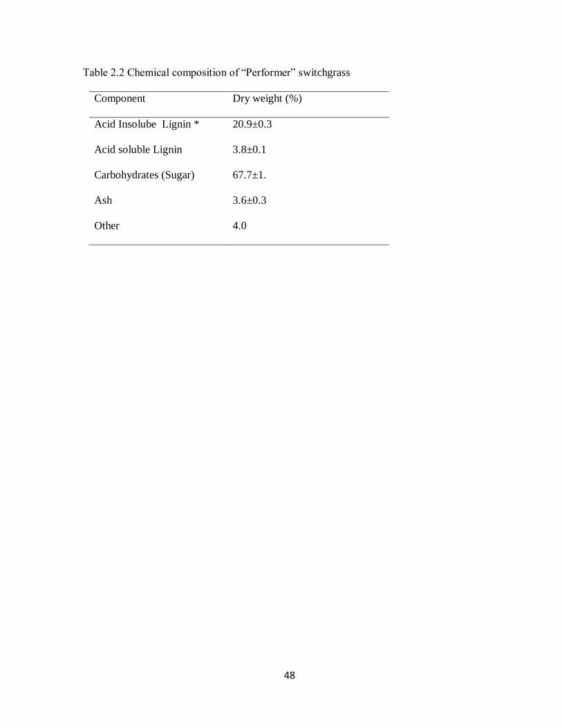
48
Table 2.2 Chemical composition of “Performer” switchgrass
Component Dry weight (%)
Acid Insolube Lignin * 20.9±0.3
Acid soluble Lignin 3.8±0.1
Carbohydrates (Sugar) 67.7±1.
Ash 3.6±0.3
Other 4.0
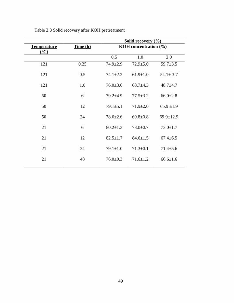
49
Table 2.3 Solid recovery after KOH pretreatment
Solid recovery (%)
Temperature
(°C)
Time (h) KOH concentration (%)
0.5 1.0 2.0
121 0.25 74.9±2.9
72.9±5.0
59.7±3.5
121 0.5 74.1±2.2
61.9±1.0
54.1± 3.7
121
1.0 76.0±3.6 68.7±4.3 48.7±4.7
50 6 79.2±4.9
77.5±3.2
66.0±2.8
50 12 79.1±5.1
71.9±2.0
65.9 ±1.9
50
24 78.6±2.6 69.8±0.8 69.9±12.9
21 6
80.2±1.3
78.0±0.7
73.0±1.7
21 12
82.5±1.7
84.6±1.5
67.4±6.5
21 24
79.1±1.0
71.3±0.1
71.4±5.6
21
48 76.0±0.3 71.6±1.2 66.6±1.6
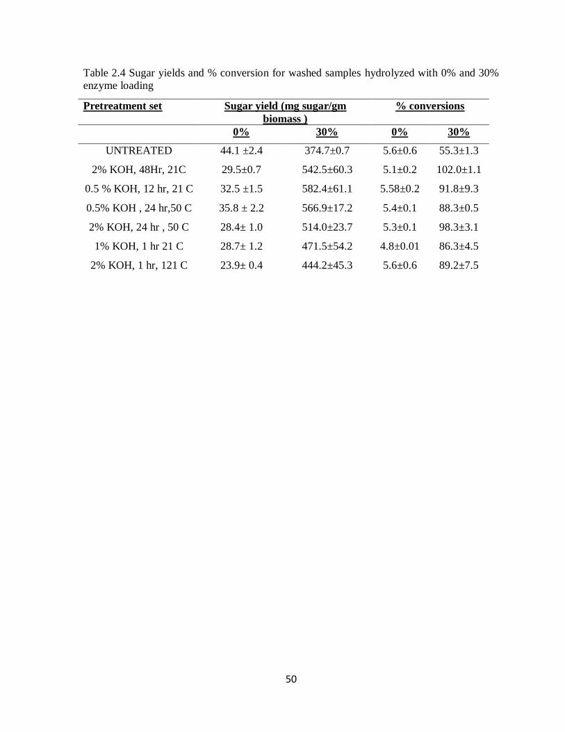
50
Table 2.4 Sugar yields and % conversion for washed samples hydrolyzed with 0% and 30%
enzyme loading
Pretreatment set Sugar yield (mg sugar/gm
biomass )
% conversions
0% 30% 0% 30%
UNTREATED 44.1 ±2.4 374.7±0.7 5.6±0.6 55.3±1.3
2% KOH, 48Hr, 21C 29.5±0.7 542.5±60.3 5.1±0.2 102.0±1.1
0.5 % KOH, 12 hr, 21 C 32.5 ±1.5 582.4±61.1 5.58±0.2 91.8±9.3
0.5% KOH , 24 hr,50 C 35.8 ± 2.2 566.9±17.2 5.4±0.1 88.3±0.5
2% KOH, 24 hr , 50 C 28.4± 1.0 514.0±23.7 5.3±0.1 98.3±3.1
1% KOH, 1 hr 21 C 28.7± 1.2 471.5±54.2 4.8±0.01 86.3±4.5
2% KOH, 1 hr, 121 C 23.9± 0.4 444.2±45.3 5.6±0.6 89.2±7.5
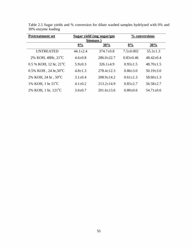
51
Table 2.5 Sugar yields and % conversion for dilute washed samples hydrlyzed with 0% and
30% enzyme loading
Pretreatment set Sugar yield (mg sugar/gm
biomass )
% conversions
0% 30% 0% 30%
UNTREATED 44.1±2.4 374.7±0.8 7.5±0.002 55.3±1.3
2% KOH, 48Hr, 21oC 4.6±0.8 286.0±22.7 0.83±0.46 48.42±0.4
0.5 % KOH, 12 hr, 21oC 5.9±0.3 326.1±4.9 0.93±1.5 48.70±1.5
0.5% KOH , 24 hr,50oC 4.8±1.3 278.4±12.3 0.86±3.0 50.19±3.0
2% KOH, 24 hr , 50oC 3.1±0.4 208.9±14.2 0.61±1.3 58.60±1.3
1% KOH, 1 hr 21oC 4.1±0.2 213.2±14.9 0.83±2.7 56.58±2.7
2% KOH, 1 hr, 121oC 3.6±0.7 201.6±13.6 0.80±0.6 54.71±0.6
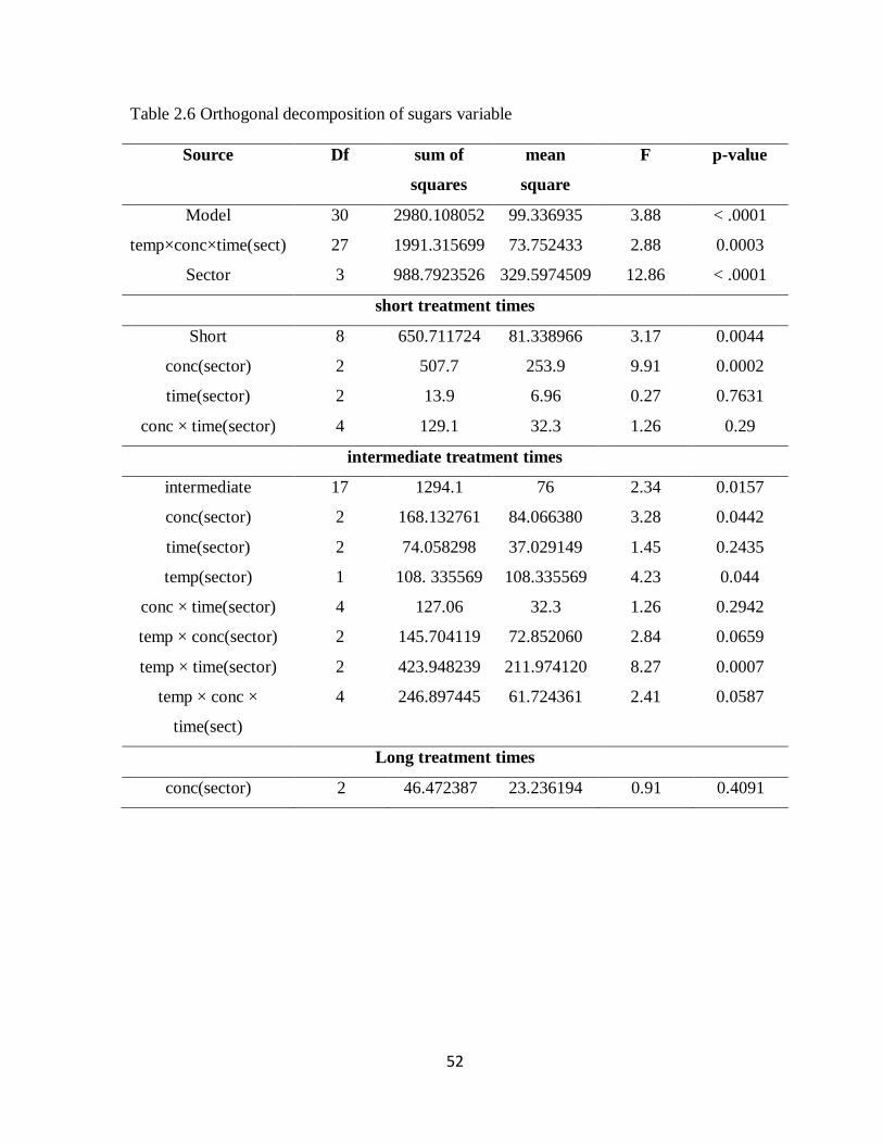
52
Table 2.6 Orthogonal decomposition of sugars variable
Source Df sum of
squares
mean
square
F p-value
Model 30 2980.108052 99.336935 3.88 < .0001
temp×conc×time(sect) 27 1991.315699 73.752433 2.88 0.0003
Sector 3 988.7923526 329.5974509 12.86 < .0001
short treatment times
Short 8 650.711724 81.338966 3.17 0.0044
conc(sector) 2 507.7 253.9 9.91 0.0002
time(sector) 2 13.9 6.96 0.27 0.7631
conc × time(sector) 4 129.1 32.3 1.26 0.29
intermediate treatment times
intermediate 17 1294.1 76 2.34 0.0157
conc(sector) 2 168.132761 84.066380 3.28 0.0442
time(sector) 2 74.058298 37.029149 1.45 0.2435
temp(sector) 1 108. 335569 108.335569 4.23 0.044
conc × time(sector) 4 127.06 32.3 1.26 0.2942
temp × conc(sector) 2 145.704119 72.852060 2.84 0.0659
temp × time(sector) 2 423.948239 211.974120 8.27 0.0007
temp × conc ×
time(sect)
4 246.897445 61.724361 2.41 0.0587
Long treatment times
conc(sector) 2 46.472387 23.236194 0.91 0.4091
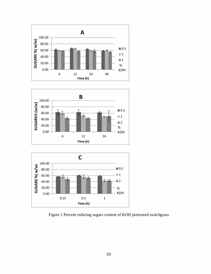
53
Figure 1 Percent reducing sugars content of KOH pretreated switchgrass
0.00
20.00
40.00
60.00
80.00
100.00
6 12 24 48
SUG
AR
S %
( w
/w)
Time (h)
A
0.5
1
2
% KOH
0.00
20.00
40.00
60.00
80.00
100.00
6 12 24
SUG
AR
S% (w
/w)
Time (h)
B
0.5
1
2
% KOH
0.00
20.00
40.00
60.00
80.00
100.00
0.25 0.5 1
SUG
AR
S %
( w
/w)
Time (h)
C
0.5
1
2
% KOH

54
Figure 2 Percent acid insoluble lignin content of KOH pretreated switchgrass
0.00
5.00
10.00
15.00
20.00
25.00
6 12 24 48
AIL
%(w
/w)
Time (h)
A
0.5
1
2
% KOH
0.00
5.00
10.00
15.00
20.00
25.00
12 24 48
AIL
%(w
/w)
Time (h)
0.5
1
2
B
% KOH
0.00
5.00
10.00
15.00
20.00
25.00
0.25 0.5 1
AIL
%(w
/w)
Time (h)
C
0.5
1
2
% KOH

55
CHAPTER 3
Effects of ultrasonication of switchgrass on fermentable sugar generation and structure
3.1 Abstract
Pretreatment of biomass for effective sugar yield has been studied extensively in the area of
bio-fuel research. The conventional methods employed to preprocess biomass for making it
conducive to better sugar yield through enzymatic hydrolysis have been hampered by some
key issues like poor energy efficiency and production of undesirable bio-products.
Ultrasonication is a method that involves the treatment of biomass through ultrasonic waves
in a liquid medium without additional chemicals. In this study the effects of ultrasonic
irradiation on switchgrass, a potential feedstock for bio ethanol production due to it high
cellulosic content were investigated.was observed. Scanning electron microscopy was
conducted to assess structural changes in pretreated samples and based on visual evidence of
disintegration and compositional analyses, samples from select pretreatment combinations
were chosen for enzymatic hydrolysis at two different enzyme loading to assess sugar
generation. Temperature controlled ultrasonication for 60 min, 100% amplitude in stainless
steel vessel , gave the highest sugar conversions of 84.6 and 84.7 % for 30% Cellic® Ctec2
and 30% Dyadic Alternafuel 200L loadings repectively. Based on the overall results, it is
inferred that ultrasonication alone is not suitable to improving sugar generation from
switchgrass and further investigation is needed.
Keywords: ultrasonication, Panicum virgatumis, amplitude, enzymatic hydrolysis, acid
insoluble lignin, scanning electron microscopy.
56
3.2 Introduction
The choice of feedstock is central to the controversy surrounding biofuels today.
Current technologies associated with the use of food as fuel and large-scale changes in land
usage have raised numerous concerns, For biofuels to have any meaningful impact on
energy, biomass feedstock must be widely available at low cost and without negative
environmental impact. Lignocelluloses - the non-food component of plants fits this
description (Mousdale, 2008). Switchgrass offers a potential alternative for lignocellulosic
biomass feedstock due to its high renewability and sugar content (Keshwani and Cheng,
2008). It however presents a need for pretreatment due to break down the lignin and disrupt
the crystalline structure of cellulose, so that enzymes can easily access and hydrolyze it
(Cadoche and Lopez, 1989; Kumar et al., 2009).
Physical pretreatments such as mechanical communiton, pyrolyisis, and steam explosion,
ammonia fibre explosion can be effective in mechanical disruption of cell wall and lignin
bonds but have proven to be energy intensive (Galbe and Zacchi, 2007, Kilzer and Broido,
1965). Chemical pretreatments involve techniques such as ozonolysis, acid hydrolysis and
alkali hydrolysis dissolve, hydrolyze or oxidize the lignin bonds to expose the carbohydrates
but are hampered by undesirable inhibitor/production and require the extensice use of
recovery agents such as water for washing and hence have proven to be cost ineffective (Sun
and Cheng, 2002; Quesada et al., 1999).Ultrasonication is a physical technique that uses ultra
high frequency sound waves to alter the molecular structure of biomass.These ultra high
frequency waves travel in a viscous flow pattern in liquid medium and create pressure
vibrations, which determine the intensity The intensity of these waves is dependent on
57
temperature of the medium, and it has been observed that increase in the temperature of the
medium decreased the intensity of sonication (Feng et al., 2011). Ultrasonication has also
been applied in biological processes for disruption of cell membranes and release of cellular
enzymes also known as sonoporation. The acoustics from an ultrasound irradiated system in
liquids have been shown to effect particles in the range of 0.15 to 100 to mm (Suslick et al.,
1991 and 1994). There is a non-linear effect of the acoustic phenomena which depends on
cavitation, defined as the growth and implosive collapse of bubbles in a liquid irradiated by
ultrasound. These implosive cavity hot spots created by the collapsing bubbles have been
reported to have temperatures of roughly 5300K, pressures of about 1720 bar, and heating
and cooling rates above 109 Ks-1
(Suslick et al., 1991 and 1994). Sun et al. (2004)
investigated the extractability of hemicelluloses from bagasse by ultrasound-assisted
extraction and found that ultrasonic treatment and sequential extractions with alkali and
alkaline peroxide under the conditions led to a release of over 90% of the original
hemicelluloses and lignin. The hemicellulosic fractions obtained after ultrasonic extraction
contained relatively low amounts of associated lignins, ranging between 0.41% and 7.36%
(Sun et al., 2004). Zhang et al. (2007) while working on developing cellulose fiber for use in
composites showed that cellulose nano fibers could be extracted from lignocellulose by the
application of high intensity ultrasonication. They showed that cellulose could be treated
with ultra high frequency sound waves to produce small fibrils at nano and micro scales.
They proposed that ultrasonic hydrodynamic forces of ultrasound produce very strong
oscillating mechanical power, which may lead to the separation of cellulose microfibrils.
This indicates that ultrasound waves impact the complex lignocellulosic matrix and there is
58
potential for more refined work in the area. (Zhang et al, 2007) An added benefit of
ultrasonication is the elimination of a toxic waste stream typically generated by conventional
chemical methods. Hence this study was undertaken, as proof-of-concept, to determine the
impact of reaction vessel construction material, treatment time, amplitude and temperature
control during ultrasonication of switchgrass on its lignin content and sugar generation
potential. The structural changes in switchgrass subjected to ultrasonication were examined
by scanning electron microscopy (SEM).
3.3 Materials and methods
3.3.1 Biomass preparation
Switchgrass for all treatments in the stainless steel beaker were obtained through an
intercropping sustainability study by Weyerhaeuser Inc., investigating cultivation of loblolly
pine (Pinus taeda L.) silviculture for solid wood products intercropped with switchgrass
(Panicum virgatum L.) for biofuels production near Dover, NC was harvested in January
2011. The biomass was dried in cloth bags at 50 oC for 48 h in a convection oven at
Metabolism Education Unit, department of Animal Science, North Carolina State University,
Raleigh, NC. Dry biomass was ground to pass a 2 mm sieve in a Willey mill. The ground
switchgrass was stored in zip-locked bags at room temperature until used. Since the
composition of the two switcgrass batches were not significantly different the results reported
here are not distinguished on the basis of batch

59
3.3.2 Compositional Analysis
Acid soluble lignin (ASL), acid insoluble lignin (AIL) in untreated and sonicated samples
was determined by methods of Sluiter et al. (2008). Briefly, a 2 step acid hydrolysis was
conducted with 72% and 4 % sulfuric acid. The solids recovered after acid hydrolysis was
used to determine AIL and the hydrolysate were used for determination of ASL and reducing
sugars. Reducing sugar analysis for untreated sonicated, and enzyme hydrolysate samples
were conducted using the dinitrotrisalicylic acid (DNS) assay (Miller, 1959, Ghose, 1987).
Ash content in untreated biomass was determined as described by standard procedure given
by National Renewable Energy Laboratory Laboratory Analytical Procedures (LAP)
established by National Renewable Energy Laboratory (Sluiter et al., 2005a).
3.3.3 Scanning electron microscopy
Scanning electron microscopy (SEM) of selected ultrasonicated samples was performed for
comparative visual analyses. The samples analyzed were i) untreated sample, ii) temperature
controlled, 10 min, stainless steel 100 % amplitude sonicated and temperature controlled, 1h
min, stainless steel, 100% amplitude combination. The analysis was conducted with Hitachi
S-3200 N SEM equipment at the Analytical Instrumental Facility (AIF), NC State University.
Two g each of the select amples were vacuum dried at 40oC for 48 h. Each sample was then
dried to 0% moisture in a liquid nitrogen drying assembly before being sputter gold coated to
be visualized through the SEM.
60
3.3.4 Pretreatment
Two different batches of Alamo switchgrass were ultrasonicated by the Hielscher 1000 hd.
Hielscher 1000 hd consisted of the following parts 1) transducer 2) booster 3) sonotorode
fuel cell 4) amplitude control unit. The epuipment generates ultrasonic frequency of 20 kHz
at 2 kW, and maximum amplitude of 170 micron. Switchgrass slurry was sonicated using the
sonotrode which is the part of the equipment that transfers the oscillations created in the
transducer. The transducer being the part where electrical signals are converted into
mechanical oscillationsPreliminary studies on ultrasonication of switchgrass were conducted
in a 150 ml glass beaker at a biomass loading of 10% in 100ml deionized water without
temperature control and stirring. This resulted in accumulation of a thick layer of biomass
around the sonotrode of the ultrasonicator leading to non-uniform effect of the ultrasonic
irradiation on the biomass. The height of the sonotrode base from the bottom of the beaker
also impacted biomass di stribution during sonication. Hence stirring of the biomass slurry
inside the glass beaker to maintain uniform effect of irradiation was introduced and the
height of the sonotrode adjusted to be closer to the bottom of the beaker. Based upon studies
on ultrasonication it was observed that with increase in temperature in the biomass dissolving
medium, the intensity of the ultrasonication waves decreased. Hence treatment with
temperature control was also included in the study (Feng et al, 2011). Experiments were
conducted to determine the impact of reaction vessel construction, treatment time, and
amplitude and temperature control during sonication on biomass composition and structure
(Table 3.1).
61
Ground switchgrass slurry at 10% solid loading in 100 ml deionized water was prepared in
150 ml glass or stainless steel beakers for sonication. A magnetic stir bar was placed in the
beaker and the beaker was placed over a magnetic stirrer. The magnetic stirrer was then
placed over a “jiffy jack” such that it was exactly below the sonotrode of the ultrasonicator
(long vertical rod suspended from the top of the instrument). Constant stirring at 150 rpm
was maintained to ensure homogeneity during various treatments. Temperature of the slurry
and power dissipated during sonication was monitored every 30 s for representative samples
using a thermocouple and power gauge, respectively. Sonication without temperature control
in the glass beaker was carried out for 5, 7.5, and 10 min at 50, 75 and 100% amplitude
(corresponding with 75, 112.5, 150 µm at the face of the sonotrode) without temperature
control. Sonication treatments in a stainless steel beaker were carried out for 5, 10 and 60
min at 50, 75 and 100% amplitude. The effect of cooling the reaction vessel was investigated
by placing the stainless steel beaker in an ice bath during sonication. The temperature during
sonication was thus maintained on average at 50oC. After treatment the jiffy Jack was
lowered and the beaker with treated sample removed. Biomass stuck to the sontrode was
recovered in a clean beaker by spraying 100ml-distilled water on it. The wash water and
recovered biomass were filtered in a Buchner funnel and flask assembly by vacuum filtration
and solids collected for determination of solid recovery via moisture content measurement of
a sub-sample at 105 oC. Five g of wet recovered biomass per replicate was dried at 40
oC in a
vacuum oven for compositional analyses.
62
3.3.5 Enzymatic hydrolysis
Enzymatic hydrolysis was carried out on select pretreated biomass to determine the effect (if
any) of structural changes in ultrasonicated switchgrass on generation of fermentable sugars.
Samples from two treatments, a) highest amplitude and longest time period and b) lowest
amplitude and shortest time period were selected for hydrolysis. Cellic® Ctec2 provided by
Novozymes NA, Franklinton and AlternaFuel 200L from Dyadic International Inc., Jupiter,
Florida were used for hydrolysis. Both enzyme cocktails are mixtures of cellulase,
hemicellulase and -Glucosidase. The samples were treated with 2 enzyme loadings each to
establish the range of sugar production. A high loading of 0.3g enzyme protein/ g dry
biomass for Cellic® Ctec2 (H1) and Dyadic AlternaFuel 200L (H2) and a low enzyme
loading corresponding with 0.1 g enzyme protein / g dry biomass for Cellic® Ctec2 (L1) and
0.05 g enzyme protein / g dry biomass for Dyadic AlternaFuel 200 L (L2). Pretreated
samples with no enzyme addition (0 g enzyme protein/ g dry biomass) and untreated samples
with the low and high enzyme loadings were hydrolyzed as controls. Hydrolysis was
conducted at a solid loading of 8% in a 20 ml solution volume made up (apart from enzyme
volume) by sodium citrate buffer as the (pH 4.9) and tetracycline hydrochloride solution
equivalent to 40µg/ml to prevent contamination of the hydrolyzate.
3.3.6 Statistical analysis
All experiments in this study were conducted in triplicate. Statistical analyses using PROC
GLM procedure for a balanced factorial design was conducted in SAS 9.2© (Cary, NC) to
determine the significance of results for the two response variables (acid insoluble lignin and
63
reducing sugar content in the treated and untreated samples) over two independent variables
(amplitude and treatment time). Results from treatments in the three reaction vessel
construction materials a) stirred glass batch, b) stainless steel batch without temperature
control and c) stainless steel batch with temperature control were also compared. The
enzymatic hydrolysis data for % conversion of carbohydrates ( represented by reducing
sugars) in the pretreated or untreated biomass to fermentable sugars in the hydrolyzate was
also statistically analyzed using one way ANOVA, with % conversion as the response
variable.
3.4 Results and discussion
First batch of untreated switchgreass used in the study contained 23.5 % AIL, 4.7 % ASL,
64.5 % total reducing sugars and 1.6% ash. The second batch of untreated switchgrass used
in this study contained 24.3 % AIL, 1.9% ASL, 69.7% total reducing sugars and 1.2% ash.
3.4.1 Effect of ultrasonication on switchgrass composition
The effect of ultrasonciation on switchgrass composition was characterized by three
parameters for the various pretreatment conditions, namely, solid recovery, acid insoluble
lignin (AIL), and total reducing sugars.
3.4.1.1 Solid recovery
Since there was no chemical degradation during ultrasonication, high solid recoveries were
observed across all pretreatement combinations. The highest solid recovery of 94% was
64
observed to for 10 min, 75% amplitude batch treatment in and the lowest was observed to be
76% for the 7.5 min, 75% amplitude combination. An average solid recovery across all
pretreatements was estimated to be 88.3%. Statistical analysis of solid recovery showed that
neither time, nor amplitude had any significant effect (p< 0.05) on solid loss.
3.4.2.2 Acid insoluble lignin
The highest average acid insoluble lignin content of 25.4 % for samples sonicated in a glass
beaker with no temperature control was observed for the 10 min, 75% amplitude treatment
and the lowest acid insoluble lignin content was observed for the 10 min, 50% amplitude
treatment resulting in 18.6 % AIL.
The highest acid insoluble lignin content for temperature controlled, sonication in the
stainless steel beaker was 22.4% observed for the 10 min 100% amplitude treatment
combination. The lowest acid insoluble lignin values for this set were observed for the
combination 10 min, 50% amplitude at 20.04%.
Statistical analysis of the data from the 3 ultrasonication strategies namely a) glass with no
temperature control, b) stainless steel without temperature control and c) stainless steel with
temperature control did not show a statistically significant (p > 0.05) difference in lignin
content among the pretreated samples. In a study conducted by Gadhe et al.,( 2006) while
utilizing a sonochemical reactor at an ultrasonic frequency of 600 kHz to generate free
radicals coupled with 4 drops of 1 N NaOH on hydrolytic lignin for 5h an increase in non
conjugated carbonyl groups and a decrease in conjugated carbonyl groups was observed.
This was indicative of degradation of the lignin polymer. These results indicated that to
65
achieve degradation of lignin extremely high ultrasonic frequencies coupled with chemical
additives and long pretreatment time are required. Hence ultrasonication of switchgrass in
this study, which utilized a maximum ultrasonic frequency of 20 kHz with no chemical
additives, did not show any significant change in the composition of samples.
3.4.1.3 Total reducing sugars
The lowest reducing sugar values for the no temperature control, batch, glass beaker
combination set, were observed for the combination ranged between 7.5 min 75% amplitude
at 46.6% and the highest reducing sugar values were observed for 10 min 75% amplitude at
70.1%.
The lowest total reducing sugar values for the no temperature control, batch, metallic beaker
set were observed for the combination, 60 min, 75% amplitude at 59.0% and the highest
reducing sugar values were observed for 5 min 50% amplitude at 67.2%.
The lowest total reducing sugar values for the no temperature control, batch, metallic beaker
set were observed for the combination 5 min 75% amplitude at 60.7% and the highest total
reducing sugar values for this set was observed for the combination, 10 min, 100% amplitude
at 67.2%.
Statistical analysis of the data from the 3 ultrasonication strategies namely a) glass with no
temperature control, b) stainless steel without temperature control and c) stainless steel with
temperature control showed a significant drop (p<0.05) in sugar content of samples from
various pretreatment combinations compared to untreated samples.
66
The loss of sugars could be explained by the dissolution effect caused by disruption of the
lignocelluloses matrix. It can be inferred that solid loss, which ranged between recoveries of
76.3%-94.6% during sonication, was primarily due to loss of reducing sugars since the
average sugar retention of the original content observed for various pretreated samples was
85%.
3.4.2 Scanning electron microscopy
To better understand and comprehend the structural changes that occurred during
ultrasonication, select switchgrass samples were observed by scanning electron microscopy
(SEM). Figure 1A depicts untreated switchgrass which shows integrity and robustness of
particles. It shows a clear and intact outer core and solid edges. In Fig 1B, which represent
samples from temperature controlled sonication in the metallic beaker for 10 minutes, it was
observed that at shorter time intervals a slight peeling away and disruption of the outer core
occurred possibly due to the collapsing of bubbles and pressure variations.When
ultrasonication was conducted for a longer time interval of 1 h in the temperature controlled
stainless steel beaker, a extensive disruption of the outer sheath and rupturing of the inner
core occured (Figs 1 C and D). These samples also show a tendency of crack formation on
the outer layer on some of the particles visualized which suggest mechanical disruption of the
outer layer through the force exerted on the particles.
These trends of mechanical disruption were in accordance with earlier studies conducted on
SEM analyses of physically pretreated lignocellulosic materials (Behera et al., 1996). There
was no evidence of pore formation or any solubulization effect on the biomass structure in
67
the ultrasonicated samples confirming the compositional analysis trends of insignificant
lignin degradation. The mechanical disruption however might have led to an increase in the
surface area of the particles rendering them effective for enzymatic hydrolysis.
3.4.3 Sugar yield after enzymatic hydrolysis
As there were no significant(p<0.05) differences in the composition of samples from various
sonication conditions, samples for hydrolysis were selected on the basis of treatment
intensity and its impact on structure which could be deduced from visual analyses through
SEM. Two samples each from both the temperature controlled and no temperature controlled
stainless steel beaker sets with one being the least intense, i.e. 50% amplitude, 5 min, stirred
and the other most intense, i.e. 100% amplitude, 1 h , stirred were chosen for enzymatic
hydrolysis.
Reducing sugars in the hydrolysates from various treatment combinations and enzyme
loadings (Table 3.3 & 3.4) investigated ranged between 467 mg/g and 511 mg/g dry
untreated biomass for H1 loading and between 455mg/g and 511mg/g for H2. H1 for the
chosen combination sets led to sugar conversion of 84.6% in the temperature controlled 60
min, 100% amplitude, stainless steel beaker sonication. The conversion of untreated
switchgrass with H1 was observed to be 73.4%. H2 led to the highest (p< 0.05) sugar
conversion of 84.7% in the temperature controlled 60 min, 100% amplitude, stainless steel
beaker and the conversion of untreated switchgrass with H2 30% loading was observed to be
81.2 %. At lower enzyme loadings of L1 and L2, conversion values of 32.1% and 10.5 %
were observed for the higher intensity sonication treatment and 25.9% and 8.9% for lower
68
intensity treatments respectively. The 0% enzyme loading yielded negligible amount of
sugars in the range of 17-22 mg/g of dry untreated biomass across all pretreatment
combinations.
One way anova analysis indicated that with H1 loading, samples drawn from temperature
controlled 60 min, 100% amplitude, stainless steel beaker combination had significantly
higher conversion values (p < 0.05) than untreated switchgrass and samples from other
treatment combinations. The statistical analysis of H1 loading samples when compared with
H2 loading showed that H1 samples the untreated samples showed significantly low
conversion value than the highest converstion treatment, whereas H2 loading samples
showed that the untreated was not significantly different (p<0.05) from the highest
conversion treatment value but was significantly higher (p<0.05) than the rest of the
treatment combinations. The L1 and L2 loadings showed the same pattern with the highest
conversion observed for the temperature controlled 60 min, 100% amplitude combination
was significantly higher (p<0.05) from all the other sets.
The pretreatment effectiveness of temperature controlled ultrasonication at higher residence
time and high amplitude showed that temperature of the liquid medium had an effect on
mechanical disruption of the lignocellulosic matrix confirming the earlier studies on the
inverse relationship between intensity of ultrasonication and temperature of medium (Feng et
al, 2010). This enhanced mechanical disruption seemed to have increased the hydrolysis
efficiency of the treatment combination.
The total sugar yields however were less than the untreated for all the treatement
combinations in both the temperature sets possibly due to loss of some sugars during
69
ultrasonication. This suggested that ultrasonication alone did not alter the structure enough to
significantly (p< 0.5) produce higher yields of reducing sugars. This observation was in
accordance with studies conducted, where a chemical additve was required to assist
ultrasonication for significantly high yields (Mazzoccoli and Paul, 2010; Montalbo-Lomboy
et al., 2010; Younus et al., 2010).
3.5 Conclusions
Based on the results on this study it can be concluded that sonication treatment at 170 micron
(100%) amplitude, for 60 min in a stainless steel beaker with temperature control was the
most effective pretreatment strategy among all the conditions tested. The high conversion
values of the untreated samples at high enzyme loading H1 and H2, need to be investigated
further. The tendency of higher enzymatic loadings in this study to generate considerably
high sugar conversion in untreated switchgrass samples presents a new direction relative to
economic viability of pretreatment and hydrolysis processes.
However ultrasonication alone did not prove to be an effective pretreatment technique
overall. The reported range of particle size that can be affected by ultrasonication (0.15 – 100
mm) is large and therefore higher particle sizes need to be explored to determine the true
potential of this technique.
Considering that ultrasonication does not provide significant change in chemical composition
of biomass, it could be utilized as preliminary pretreatment step to decrease the severity of a
primary pretreatment method. In this study a tendency of the opening up of the biomass

70
structure through mechanical disruption and this could be utilized to assist biological
treatments which have longer residence times (Yu et al., 2009).
3.6 Acknowledgements
This material is based upon work supported by the Department of Energy under Award
Number GO88053.
The authors would like to thank Dr. Joe Burns, Department of Crop Science, NCSU and Dr.
Zakiya H. Leggett, Weyerhaeuser Company (Southern Timberlands RandD) for assistance in
obtaining the switchgrass.
Disclaimer: This report was prepared as an account of work sponsored by an agency of the
United States Government. Neither the United States Government nor any agency thereof,
nor any of their employees, makes any warranty, express or implied, or assumes any legal
liability or responsibility for the accuracy, completeness, or usefulness of any information,
apparatus, product, or process disclosed, or represents that its use would not infringe
privately owned rights. Reference herein to any specific commercial product, process, or
service by trade name, trademark, manufacturer, or otherwise does not necessarily constitute
or imply its endorsement, recommendation, or favoring by the United States Government or
any agency thereof. The views and opinions of authors expressed herein do not necessarily
state or reflect those of the United States Government or any agency thereof.
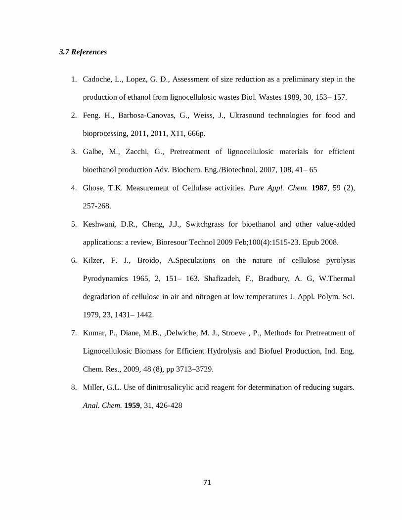
71
3.7 References
1. Cadoche, L., Lopez, G. D., Assessment of size reduction as a preliminary step in the
production of ethanol from lignocellulosic wastes Biol. Wastes 1989, 30, 153– 157.
2. Feng. H., Barbosa-Canovas, G., Weiss, J., Ultrasound technologies for food and
bioprocessing, 2011, 2011, X11, 666p.
3. Galbe, M., Zacchi, G., Pretreatment of lignocellulosic materials for efficient
bioethanol production Adv. Biochem. Eng./Biotechnol. 2007, 108, 41– 65
4. Ghose, T.K. Measurement of Cellulase activities. Pure Appl. Chem. 1987, 59 (2),
257-268.
5. Keshwani, D.R., Cheng, J.J., Switchgrass for bioethanol and other value-added
applications: a review, Bioresour Technol 2009 Feb;100(4):1515-23. Epub 2008.
6. Kilzer, F. J., Broido, A.Speculations on the nature of cellulose pyrolysis
Pyrodynamics 1965, 2, 151– 163. Shafizadeh, F., Bradbury, A. G, W.Thermal
degradation of cellulose in air and nitrogen at low temperatures J. Appl. Polym. Sci.
1979, 23, 1431– 1442.
7. Kumar, P., Diane, M.B., ,Delwiche, M. J., Stroeve , P., Methods for Pretreatment of
Lignocellulosic Biomass for Efficient Hydrolysis and Biofuel Production, Ind. Eng.
Chem. Res., 2009, 48 (8), pp 3713–3729.
8. Miller, G.L. Use of dinitrosalicylic acid reagent for determination of reducing sugars.
Anal. Chem. 1959, 31, 426-428
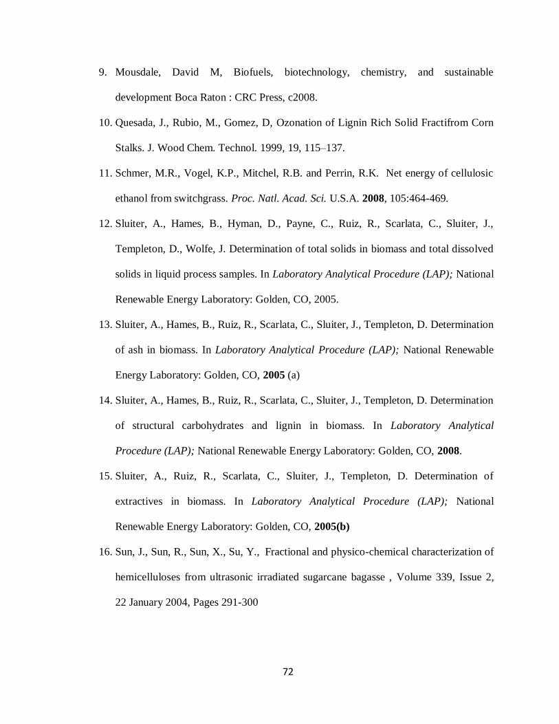
72
9. Mousdale, David M, Biofuels, biotechnology, chemistry, and sustainable
development Boca Raton : CRC Press, c2008.
10. Quesada, J., Rubio, M., Gomez, D, Ozonation of Lignin Rich Solid Fractifrom Corn
Stalks. J. Wood Chem. Technol. 1999, 19, 115–137.
11. Schmer, M.R., Vogel, K.P., Mitchel, R.B. and Perrin, R.K. Net energy of cellulosic
ethanol from switchgrass. Proc. Natl. Acad. Sci. U.S.A. 2008, 105:464-469.
12. Sluiter, A., Hames, B., Hyman, D., Payne, C., Ruiz, R., Scarlata, C., Sluiter, J.,
Templeton, D., Wolfe, J. Determination of total solids in biomass and total dissolved
solids in liquid process samples. In Laboratory Analytical Procedure (LAP); National
Renewable Energy Laboratory: Golden, CO, 2005.
13. Sluiter, A., Hames, B., Ruiz, R., Scarlata, C., Sluiter, J., Templeton, D. Determination
of ash in biomass. In Laboratory Analytical Procedure (LAP); National Renewable
Energy Laboratory: Golden, CO, 2005 (a)
14. Sluiter, A., Hames, B., Ruiz, R., Scarlata, C., Sluiter, J., Templeton, D. Determination
of structural carbohydrates and lignin in biomass. In Laboratory Analytical
Procedure (LAP); National Renewable Energy Laboratory: Golden, CO, 2008.
15. Sluiter, A., Ruiz, R., Scarlata, C., Sluiter, J., Templeton, D. Determination of
extractives in biomass. In Laboratory Analytical Procedure (LAP); National
Renewable Energy Laboratory: Golden, CO, 2005(b)
16. Sun, J., Sun, R., Sun, X., Su, Y., Fractional and physico-chemical characterization of
hemicelluloses from ultrasonic irradiated sugarcane bagasse , Volume 339, Issue 2,
22 January 2004, Pages 291-300
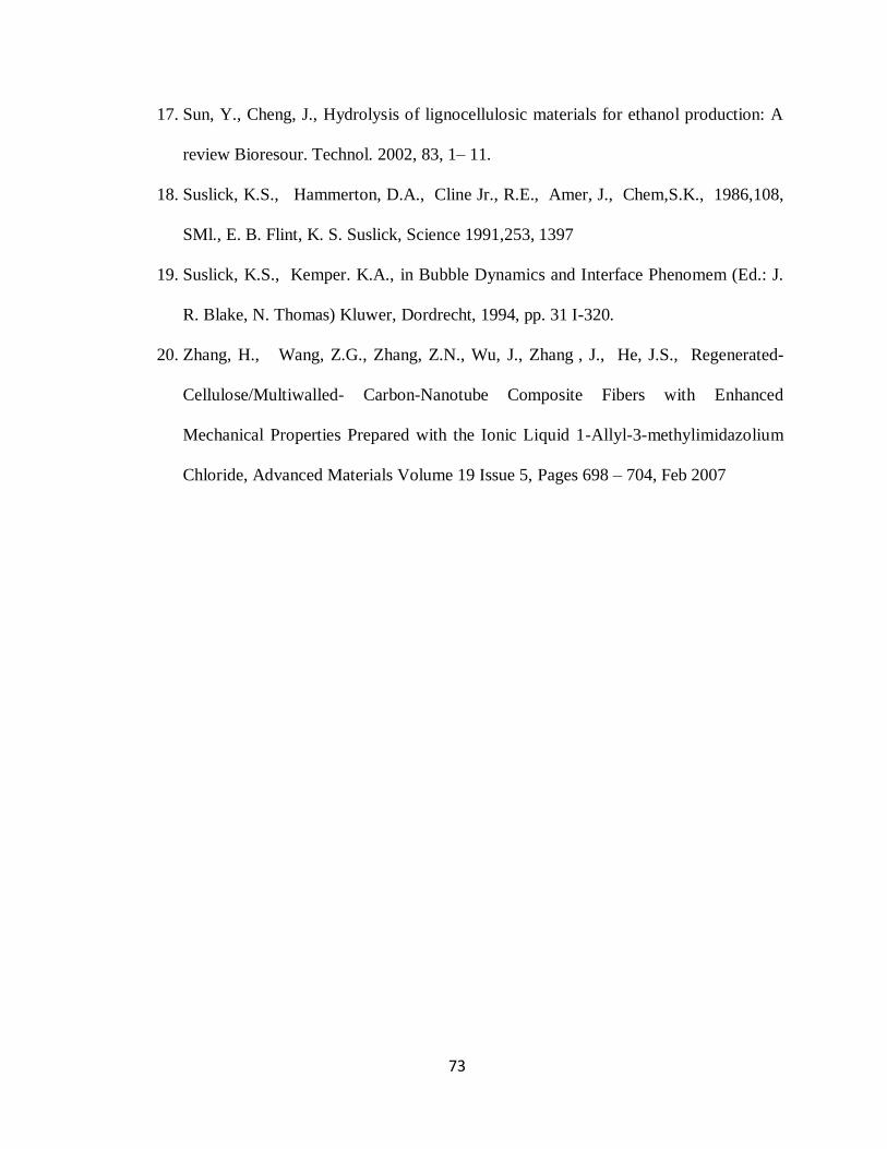
73
17. Sun, Y., Cheng, J., Hydrolysis of lignocellulosic materials for ethanol production: A
review Bioresour. Technol. 2002, 83, 1– 11.
18. Suslick, K.S., Hammerton, D.A., Cline Jr., R.E., Amer, J., Chem,S.K., 1986,108,
SMl., E. B. Flint, K. S. Suslick, Science 1991,253, 1397
19. Suslick, K.S., Kemper. K.A., in Bubble Dynamics and Interface Phenomem (Ed.: J.
R. Blake, N. Thomas) Kluwer, Dordrecht, 1994, pp. 31 I-320.
20. Zhang, H., Wang, Z.G., Zhang, Z.N., Wu, J., Zhang , J., He, J.S., Regenerated-
Cellulose/Multiwalled- Carbon-Nanotube Composite Fibers with Enhanced
Mechanical Properties Prepared with the Ionic Liquid 1-Allyl-3-methylimidazolium
Chloride, Advanced Materials Volume 19 Issue 5, Pages 698 – 704, Feb 2007
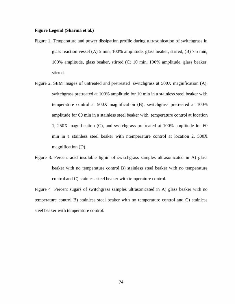
74
Figure Legend (Sharma et al.)
Figure 1. Temperature and power dissipation profile during ultrasonication of switchgrass in
glass reaction vessel (A) 5 min, 100% amplitude, glass beaker, stirred, (B) 7.5 min,
100% amplitude, glass beaker, stirred (C) 10 min, 100% amplitude, glass beaker,
stirred.
Figure 2. SEM images of untreated and pretreated switchgrass at 500X magnification (A),
switchgrass pretreated at 100% amplitude for 10 min in a stainless steel beaker with
temperature control at 500X magnification (B), switchgrass pretreated at 100%
amplitude for 60 min in a stainless steel beaker with temperature control at location
1, 250X magnification (C), and switchgrass pretreated at 100% amplitude for 60
min in a stainless steel beaker with ntemperature control at location 2, 500X
magnification (D).
Figure 3. Percent acid insoluble lignin of switchgrass samples ultrasonicated in A) glass
beaker with no temperature control B) stainless steel beaker with no temperature
control and C) stainless steel beaker with temperature control.
Figure 4 Percent sugars of switchgrass samples ultrasonicated in A) glass beaker with no
temperature control B) stainless steel beaker with no temperature control and C) stainless
steel beaker with temperature control.
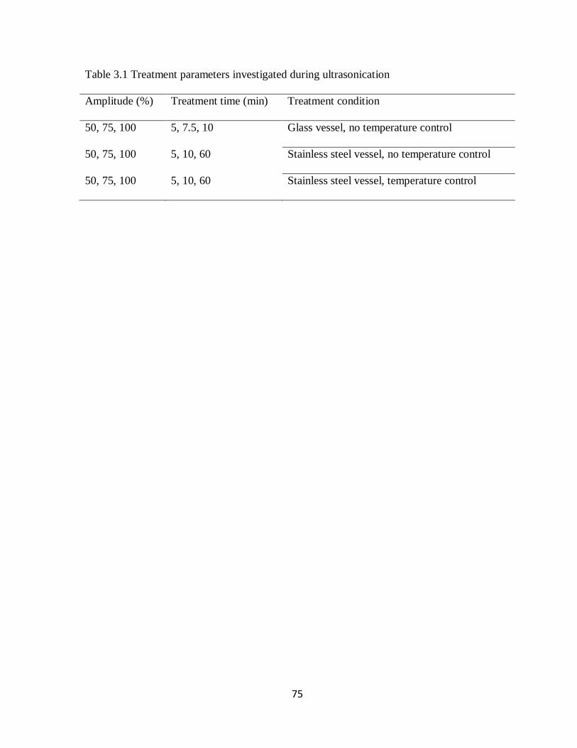
75
Table 3.1 Treatment parameters investigated during ultrasonication
Amplitude (%) Treatment time (min) Treatment condition
50, 75, 100 5, 7.5, 10 Glass vessel, no temperature control
50, 75, 100 5, 10, 60 Stainless steel vessel, no temperature control
50, 75, 100 5, 10, 60 Stainless steel vessel, temperature control
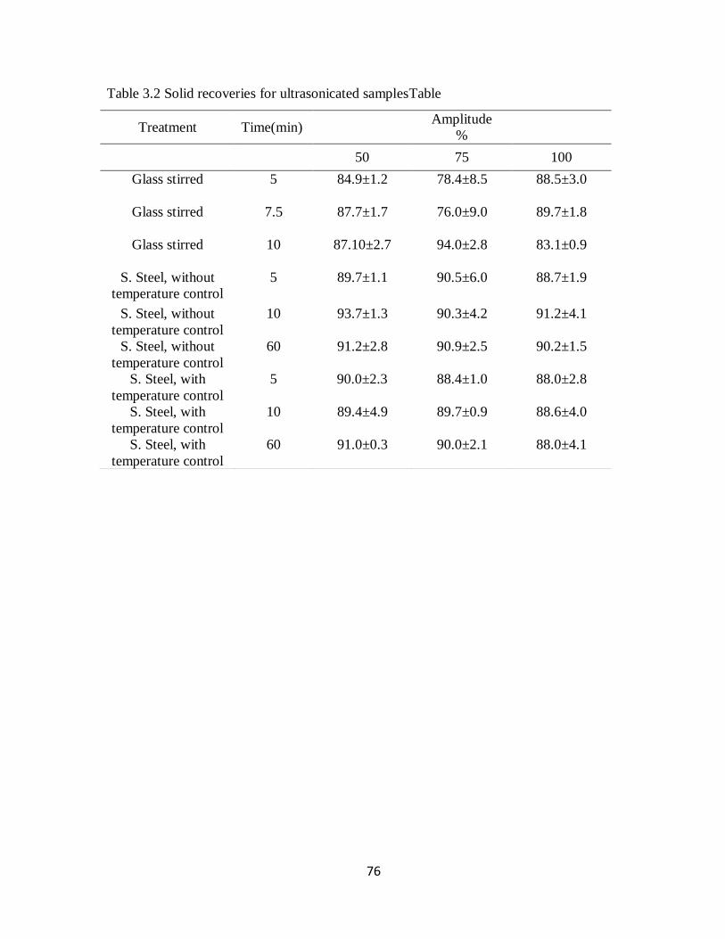
76
Table 3.2 Solid recoveries for ultrasonicated samplesTable
Treatment Time(min) Amplitude
%
50 75 100
Glass stirred 5 84.9±1.2
78.4±8.5
88.5±3.0
Glass stirred 7.5 87.7±1.7
76.0±9.0
89.7±1.8
Glass stirred 10 87.10±2.7 94.0±2.8 83.1±0.9
S. Steel, without
temperature control
5
89.7±1.1
90.5±6.0
88.7±1.9
S. Steel, without
temperature control
10 93.7±1.3
90.3±4.2
91.2±4.1
S. Steel, without
temperature control
60 91.2±2.8 90.9±2.5 90.2±1.5
S. Steel, with
temperature control
5
90.0±2.3
88.4±1.0
88.0±2.8
S. Steel, with
temperature control
10 89.4±4.9
89.7±0.9
88.6±4.0
S. Steel, with
temperature control
60 91.0±0.3
90.0±2.1
88.0±4.1
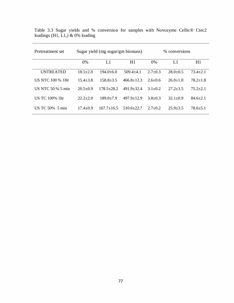
77
Table 3.3 Sugar yields and % conversion for samples with Novozyme Cellic® Ctec2
loadings (H1, L1,) & 0% loading
Pretreatment set
Sugar yield (mg sugar/gm biomass)
% conversions
0% L1 H1 0% L1 H1
UNTREATED 18.5±2.0 194.0±6.0 509.4±4.1 2.7±0.3 28.0±0.5 73.4±2.1
US NTC 100 % 1Hr 15.4±3.8 158.8±3.5 466.8±12.3 2.6±0.6 26.0±1.0 78.2±1.8
US NTC 50 % 5 min 20.5±0.9 178.5±28.2 491.9±32.4 3.1±0.2 27.2±3.5 75.2±2.1
US TC 100% 1hr 22.2±2.0 189.0±7.9 497.9±12.9 3.8±0.3 32.1±0.9 84.6±2.1
US TC 50% 5 min 17.4±0.9 167.7±16.5 510.6±22.7 2.7±0.2 25.9±3.5 78.6±5.1
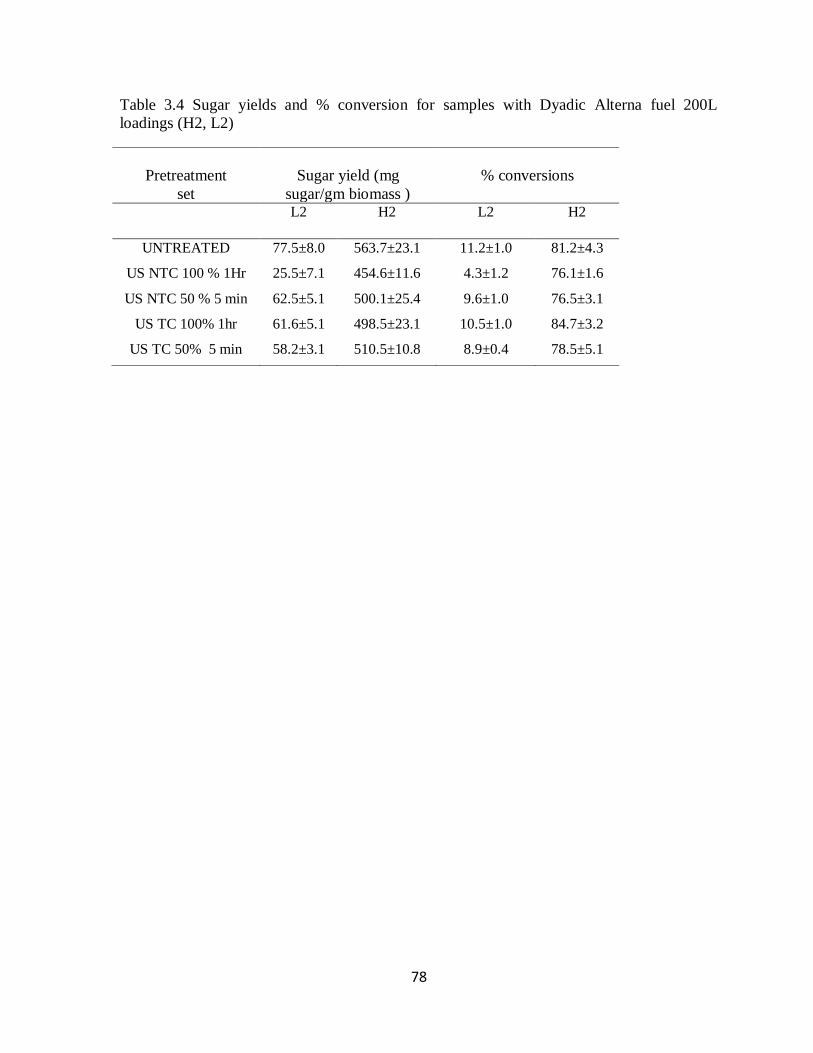
78
Table 3.4 Sugar yields and % conversion for samples with Dyadic Alterna fuel 200L
loadings (H2, L2)
Pretreatment
set
Sugar yield (mg
sugar/gm biomass )
% conversions
L2
H2 L2 H2
UNTREATED 77.5±8.0 563.7±23.1 11.2±1.0 81.2±4.3
US NTC 100 % 1Hr 25.5±7.1 454.6±11.6 4.3±1.2 76.1±1.6
US NTC 50 % 5 min 62.5±5.1 500.1±25.4 9.6±1.0 76.5±3.1
US TC 100% 1hr 61.6±5.1 498.5±23.1 10.5±1.0 84.7±3.2
US TC 50% 5 min 58.2±3.1 510.5±10.8 8.9±0.4 78.5±5.1
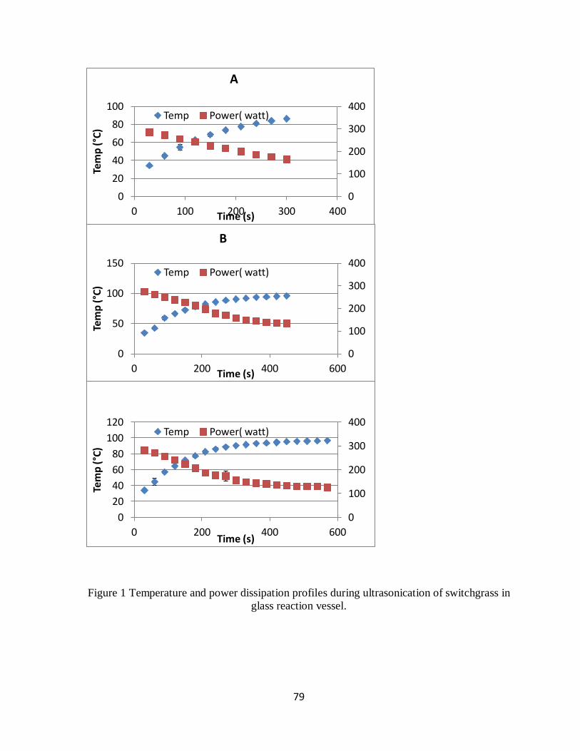
79
Figure 1 Temperature and power dissipation profiles during ultrasonication of switchgrass in
glass reaction vessel.
0
100
200
300
400
0
20
40
60
80
100
0 100 200 300 400
Tem
p (
°C)
Time (s)
A
Temp Power( watt)
0
100
200
300
400
0
50
100
150
0 200 400 600
Tem
p (
°C)
Time (s)
B
Temp Power( watt)
0
100
200
300
400
0
20
40
60
80
100
120
0 200 400 600
Tem
p (
°C)
Time (s)
Temp Power( watt)

80
Figure 2 SEM images of untreated and pretreated switchgrass
A B
D C
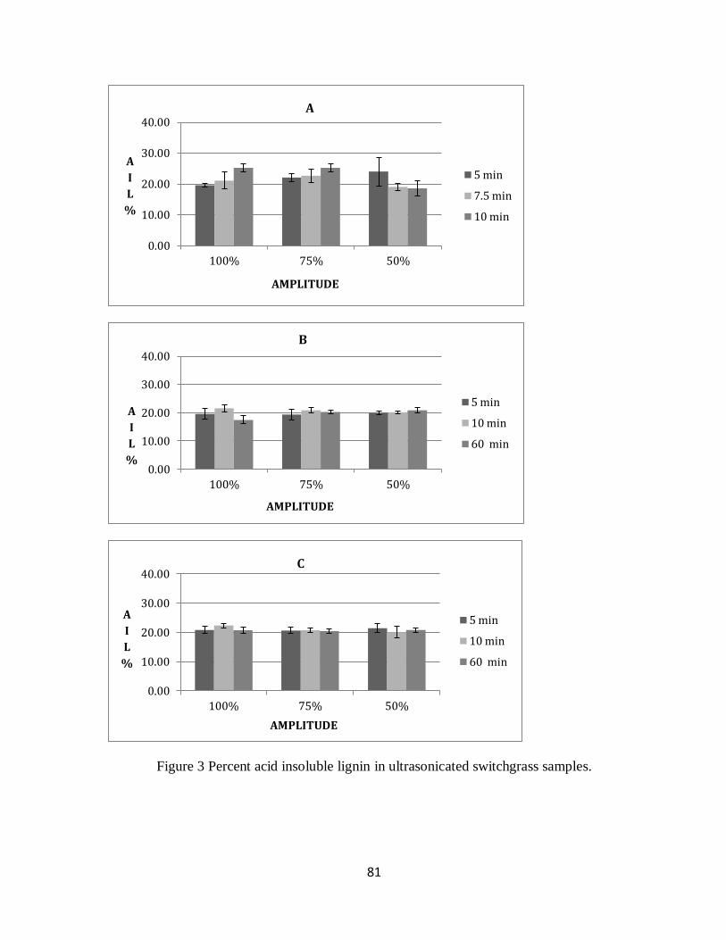
81
Figure 3 Percent acid insoluble lignin in ultrasonicated switchgrass samples.
0.00
10.00
20.00
30.00
40.00
100% 75% 50%
A
I
L
%
AMPLITUDE
5 min
7.5 min
10 min
A
0.00
10.00
20.00
30.00
40.00
100% 75% 50%
A
I
L
%
AMPLITUDE
5 min
10 min
60 min
B
0.00
10.00
20.00
30.00
40.00
100% 75% 50%
A
I
L
%
AMPLITUDE
5 min
10 min
60 min
C
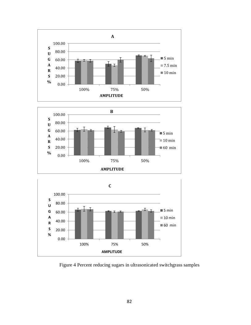
82
Figure 4 Percent reducing sugars in ultrasonicated switchgrass samples
0.00
20.00
40.00
60.00
80.00
100.00
100% 75% 50%
S
U
G
A
R
S
%
AMPLITUDE
5 min
7.5 min
10 min
A
0.00
20.00
40.00
60.00
80.00
100.00
100% 75% 50%
S
U
G
A
R
S
%
AMPLITUDE
5 min
10 min
60 min
B
0.00
20.00
40.00
60.00
80.00
100.00
100% 75% 50%
S
U
G
A
R
S
%
AMPLITUDE
5 min
10 min
60 min
C
83
CHAPTER 4
Conclusions and future scope of work
With the ever increasing demand for alternative and renewable sources of energy, conversion
of starch or sugar based biomass feedstocks for sugar generation has played an important role
in the realm of bio-fuels. However, these feedstocks also cannot meet all our fuel needs.
Hence, lignocellulosic feedstocks have been explored for conversion to sugar for
fermentation. Such feedstocks require an additional pretreatment step to make them
accessible to hydrolytic enzymes.
With constant advances in the usage of different physical, chemical and biological methods
to treat carbohydrate rich lignocellulosic biomass, the challenge now is to come up with
refined methods to circumvent issues like generation of significant waste streams.
In this study of a physical and a chemical pretreatment method, relatively less utilized modes
of affecting biomass structure for sugar generation were explored.
The key conclusions of the study were:
(1) All KOH pretreatment combinations resulted in an average of 85% released
conversion of carbohydrates present in the biomass.
(2) The highest carbohydrate conversion (based on reducing sugar contents) was
observed for the combination of 2% KOH, 12 h, and 21 C. However, the 0.5% KOH,
24 h, 21 C combination proved to be the most effective utilizing the least amount of
KOH and giving a sugar yield of 582.4 mg/g with a corresponding released sugar
conversion of 91.8% , with a high enzymatic loading of 0.3 Cellic® Ctec 2 g enzyme
/ g biomass.
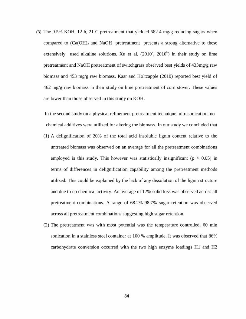
84
(3) The 0.5% KOH, 12 h, 21 C pretreatment that yielded 582.4 mg/g reducing sugars when
compared to (Ca(OH)2 and NaOH pretreatment presents a strong alternative to these
extensively used alkaline solutions. Xu et al. (2010a, 2010
b) in their study on lime
pretreatment and NaOH pretreatment of switchgrass observed best yields of 433mg/g raw
biomass and 453 mg/g raw biomass. Kaar and Holtzapple (2010) reported best yield of
462 mg/g raw biomass in their study on lime pretreatment of corn stover. These values
are lower than those observed in this study on KOH.
In the second study on a physical refinement pretreatment technique, ultrasonication, no
chemical additives were utilized for altering the biomass. In our study we concluded that
(1) A delignification of 20% of the total acid insoluble lignin content relative to the
untreated biomass was observed on an average for all the pretreatment combinations
employed is this study. This however was statistically insignificant (p > 0.05) in
terms of differences in delignification capability among the pretreatment methods
utilized. This could be explained by the lack of any dissolution of the lignin structure
and due to no chemical activity. An average of 12% solid loss was observed across all
pretreatment combinations. A range of 68.2%-98.7% sugar retention was observed
across all pretreatment combinations suggesting high sugar retention.
(2) The pretreatment was with most potential was the temperature controlled, 60 min
sonication in a stainless steel container at 100 % amplitude. It was observed that 86%
carbohydrate conversion occurred with the two high enzyme loadings H1 and H2
85
(0.3g enzyme protein/ g dry biomass of Cellc® Ctec2 and Dyadic Alternafuel 200L
respectively).
(3) It must be noted that high carbohydrate conversions occurred during hydrolysis of
untreated carbohydrate biomass potentially due to the high enzyme loading of 0.3 g
enzyme protein/ g dry biomass. The sugar yields were observed to be 375.5 for
performer switchgrass and 509.9 for Alamo.
References
1. Kaar, W.E., Holtzapple, M.T., using lime pretreatment to facilitate the enzymatic
hydrolysis of corn stover, Biomass and Bioenergy 18 (2000) 189-99.
2. Xu, J., Cheng, J.J., Sharma-Shivappa, R.R. and Burns, J.C. Lime pretreatment of
switchgrass at mild temperatures for ethanol production. Bioresource Technology.
2010,101,2900-290.

86
APPENDICES
87
APPENDIX 1
Scanning electron microscopy for Chapter 3
Introduction
The compositional analyses of ultrasonicated samples and the subsequent statistical analyses
showed that ultrasonic irradiation did not significantly degrade the ligno-cellulosic
molecules. This can be explained as ultrasonication is a purely physical treatment, thus the
possibility of any chemical reactions taking place, when the solvent is double de-ionized
distilled water are minimal. This led to the examination of any structural changes that may
have taken place relative to increase in surface area, disruption of the biomass and breaking
or loosening off of the outer crust of the biomass structure. Hence scanning electron
microscopy analysis was performed on select samples.
Material and methods
SEM analysis was conducted with Hitachi S-3200 N SEM equipment at the Analytical
Instrumental Facility (AIF), NC State University. Two g each of the selected samples for
analysis was vacuum dried at 40oC for 48 h. Each sample was then dried to 0% moisture with
liquid nitrogen drying apparatus before being sputter gold coated to be visualized through the
SEM.
The samples were drawn from the following treatment combinations:

88
1. Untreated Panicum virgatum L sample: This category of images that analyzes untreated
switchgrass in fig (a) clearly depicts integrity and robustness of particles. When
magnified to 100x and 500X it shows a clear and intact outer core and solid edges
2. Temperature controlled batch, stirred sample slurry in DIW at 10% solid loading: Fig b
and c indicate that at lower time intervals we see slight peeling away of the outer core
and at hollow tubular exposure at the edges, as we move to a longer time interval of 1 h
we see complete disruption of the outer sheath and rupturing of the inner core. These
samples also show a tendency of physical disruption on the surface.
3. No temperature control,stirred continuous recirculated sample slurry in DIW with 3%
solid loading: These category of images (fig d), suggest similar patterns like fig b & c,
with peeling away at the edges and irregular crack formation but less profound which
suggest that direct exposure and higer loading may have impacted uniform action of the
ultrasonication irradiation.
4. No temperature control,stirred continuous recirculated sample slurry in 0.5% NaOH
(w/v) solution with 3% solid loading (fig e) show clear signs of degradation of the outer
layer by a chemical dissolution effect but in very mild proportions as most of the particles
seem to retain their integrity. This may be due to disintegration of NaOH during
sonication and thus limited attack on biomass.
5. Unsonicated, stirred slurry in 0.5% NaOH (w/v) with 10% solid loading show an
increased chemical treatment effect where the outer layers seem to have been degraded
and clear regular shaped pore formation is observed. This could be attributed to higher

89
loading and direct impact of the stirring for a prolonged period where NaOH seemed to
have uniformly impacted the biomass.
Scanning electron microscopy provided insight into the structural changes that may have
taken place during the pretreatment process. It supplemented compositional analyses data
which could not provide significant information on the bio-chemical or physical changes
taking place in the biomass. SEM images helped to deduce clear outer layer degradation and
inner core disruption in some of the treatment sets not involving any chemical addition,
suggesting that such visible disruption may have lead to an increase in the surface area of
particles as well some loss in crystallinity of the cellulosic material but not enough to
significantly enhance enzymatic attachment and subsequent digestion to generate sugars.
The various SEM image acquired for switchgrass samples treated at various ultrasonication
conditions are provided below:
Figure A) untreated alamo switchgrass at magnification 100x and 500x
Figure B) Temperature controlled batch in stainless steel container at 10% solid
loading sonicated for 10 min with 100% amplitude 100x and 500x
magnification.
Figure C) 1 hr, 100% amplitude, batch temperature controlled, stainless steel at
50x and 100x magnification.
Figure D) 1 hr, 100% amplitude, 3% loading, recirculated, diw slurry ,100x and
500x magnification

90
Figure E) No temepeature control., 0.5 % NaOH , 1 hr, 100% amplitude, 3% loading,
recirculated, 30x, 100x,
Figure F) 0.5 % NaOH, no sonication, 1 hr, stirred, no temperature control at
100 x, and 500x .
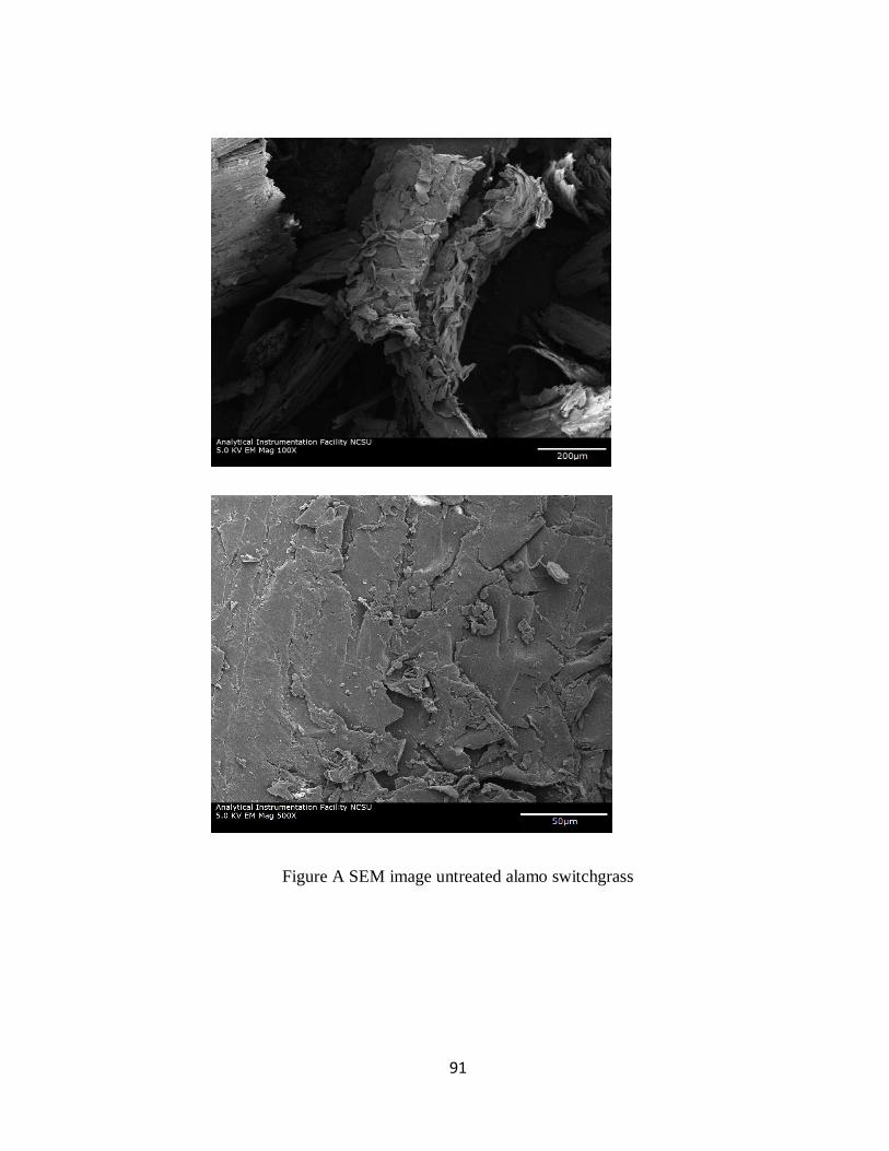
91
Figure A SEM image untreated alamo switchgrass
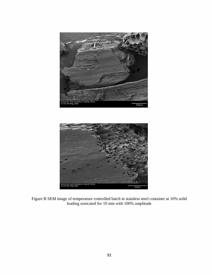
92
Figure B SEM image of temperature controlled batch in stainless steel container at 10% solid
loading sonicated for 10 min with 100% amplitude
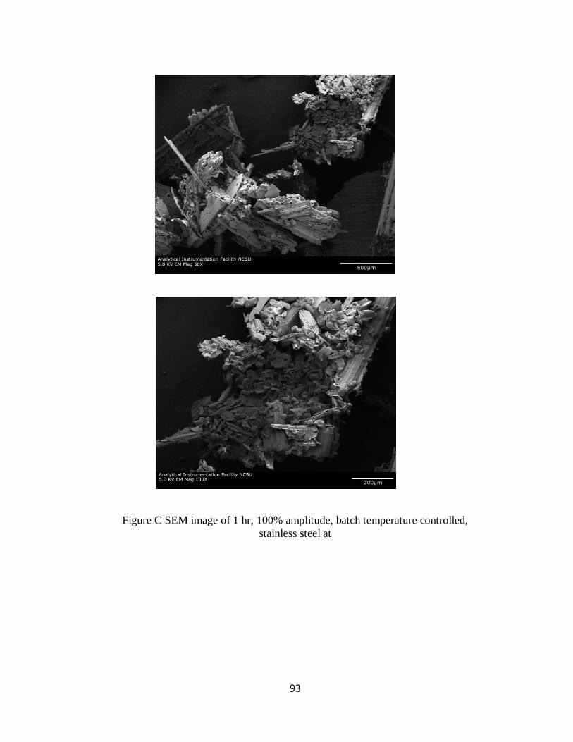
93
Figure C SEM image of 1 hr, 100% amplitude, batch temperature controlled,
stainless steel at
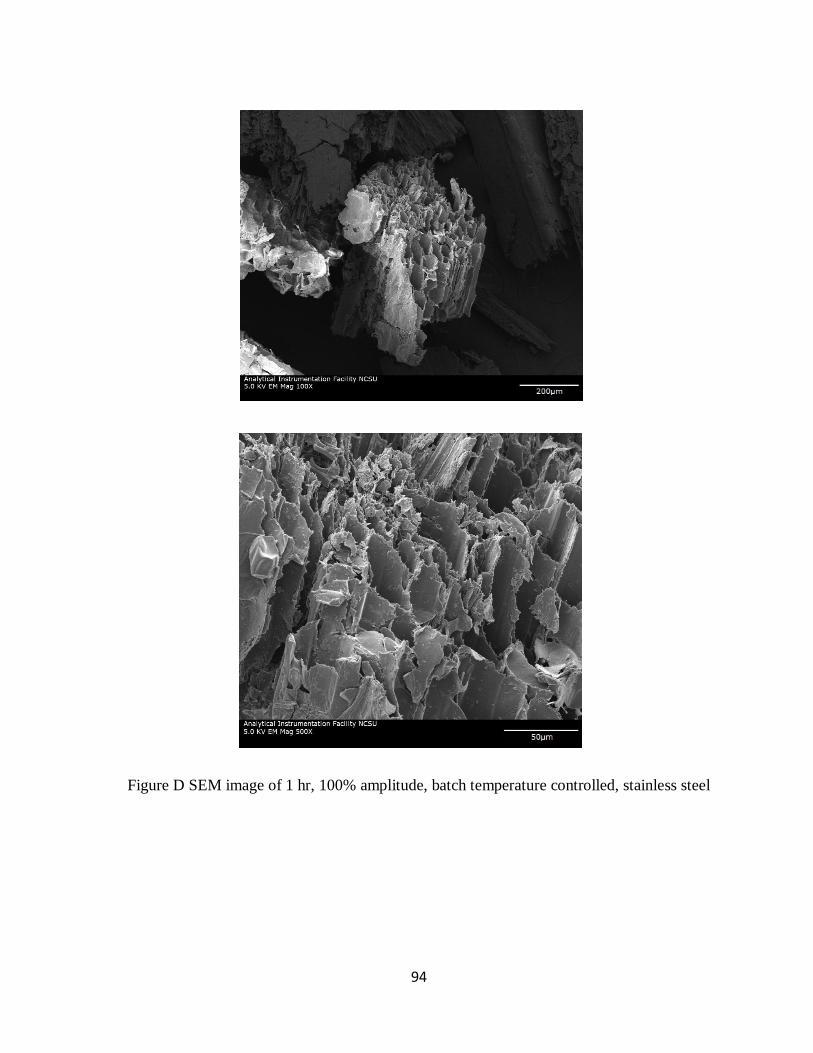
94
Figure D SEM image of 1 hr, 100% amplitude, batch temperature controlled, stainless steel
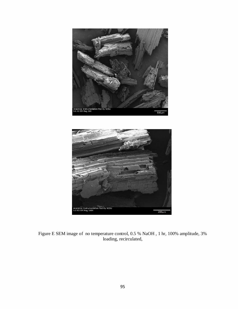
95
Figure E SEM image of no temperature control, 0.5 % NaOH , 1 hr, 100% amplitude, 3%
loading, recirculated,
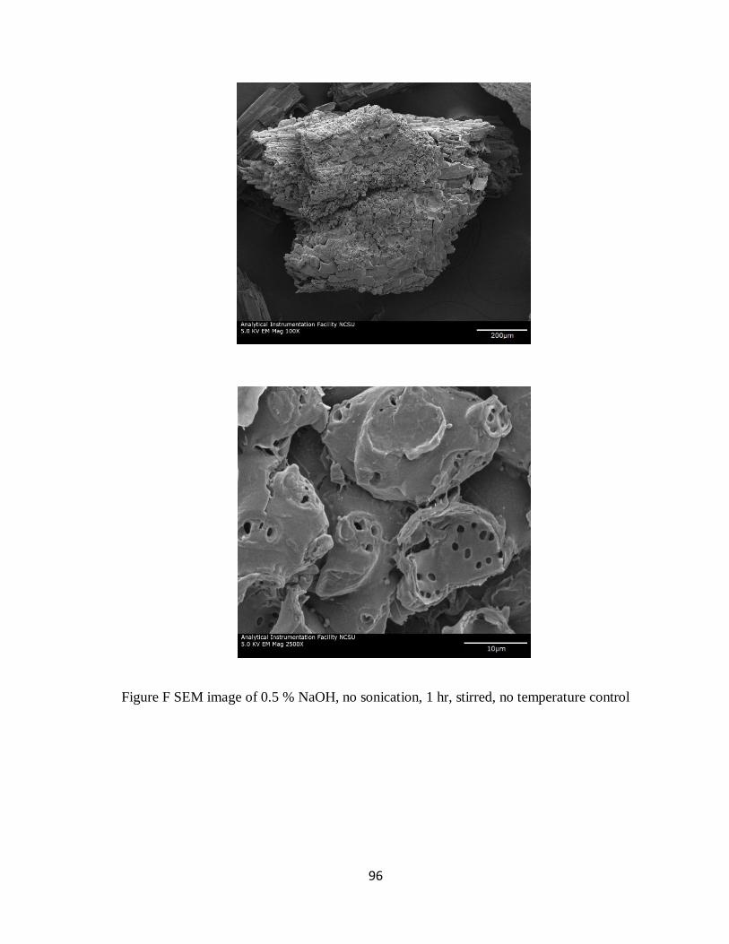
96
Figure F SEM image of 0.5 % NaOH, no sonication, 1 hr, stirred, no temperature control
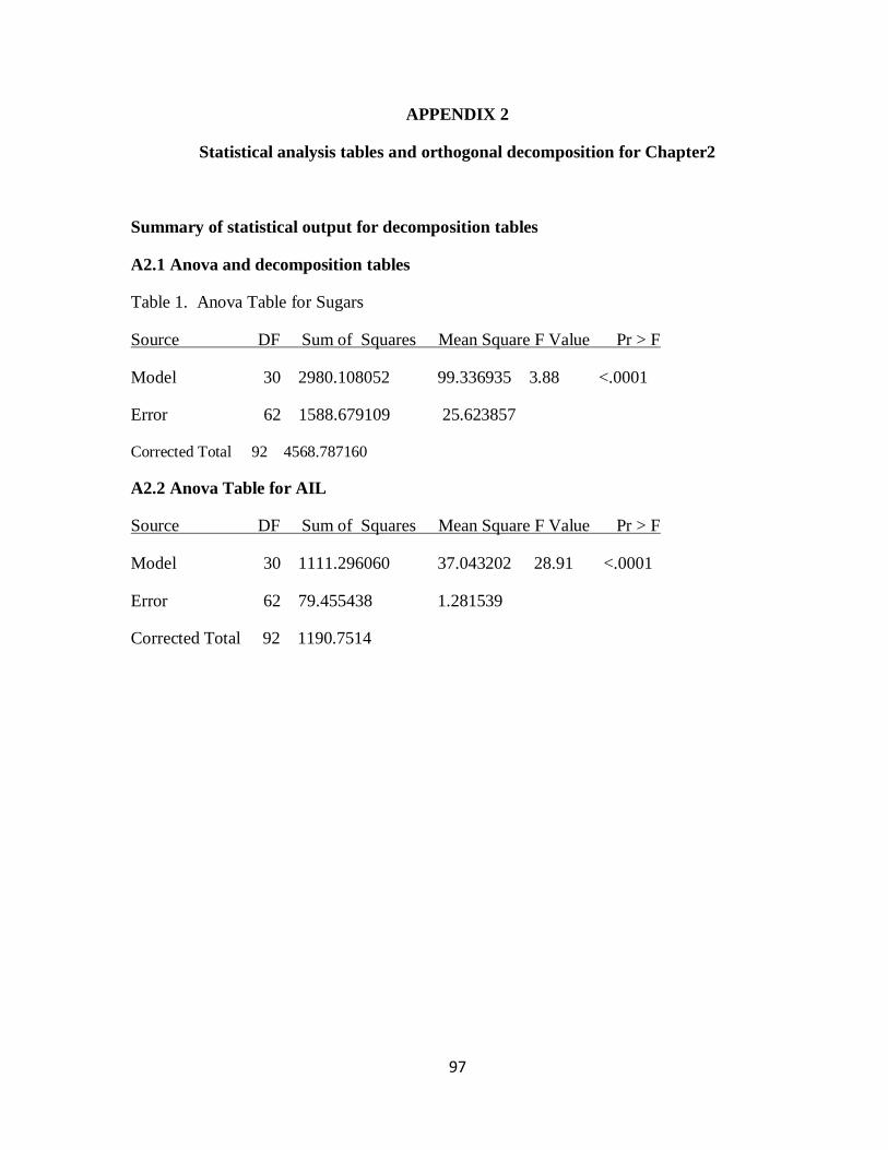
97
APPENDIX 2
Statistical analysis tables and orthogonal decomposition for Chapter2
Summary of statistical output for decomposition tables
A2.1 Anova and decomposition tables
Table 1. Anova Table for Sugars
Source DF Sum of Squares Mean Square F Value Pr > F
Model 30 2980.108052 99.336935 3.88 <.0001
Error 62 1588.679109 25.623857
Corrected Total 92 4568.787160
A2.2 Anova Table for AIL
Source DF Sum of Squares Mean Square F Value Pr > F
Model 30 1111.296060 37.043202 28.91 <.0001
Error 62 79.455438 1.281539
Corrected Total 92 1190.7514
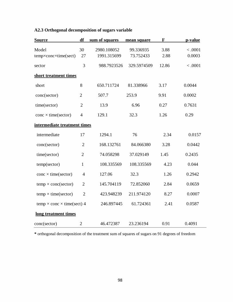
98
A2.3 Orthogonal decomposition of sugars variable
Source df sum of squares mean square F p-value
Model 30 2980.108052 99.336935 3.88 < .0001
temp×conc×time(sect) 27 1991.315699 73.752433 2.88 0.0003
sector 3 988.7923526 329.5974509 12.86 < .0001
short treatment times
short 8 650.711724 81.338966 3.17 0.0044
conc(sector) 2 507.7 253.9 9.91 0.0002
time(sector) 2 13.9 6.96 0.27 0.7631
conc × time(sector) 4 129.1 32.3 1.26 0.29
intermediate treatment times
intermediate 17 1294.1 76 2.34 0.0157
conc(sector) 2 168.132761 84.066380 3.28 0.0442
time(sector) 2 74.058298 37.029149 1.45 0.2435
temp(sector) 1 108.335569 108.335569 4.23 0.044
conc × time(sector) 4 127.06 32.3 1.26 0.2942
temp × conc(sector) 2 145.704119 72.852060 2.84 0.0659
temp × time(sector) 2 423.948239 211.974120 8.27 0.0007
temp × conc × time(sect) 4 246.897445 61.724361 2.41 0.0587
long treatment times
conc(sector) 2 46.472387 23.236194 0.91 0.4091
* orthogonal decomposition of the treatment sum of squares of sugars on 91 degrees of freedom
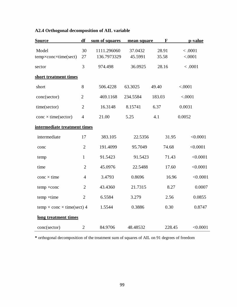
99
A2.4 Orthogonal decomposition of AIL variable
Source df sum of squares mean square F p-value
Model 30 1111.296060 37.0432 28.91 < .0001
temp×conc×time(sect) 27 136.7973329 45.5991 35.58 <.0001
sector 3 974.498 36.0925 28.16 < .0001
short treatment times
short 8 506.4228 63.3025 49.40 <.0001
conc(sector) 2 469.1168 234.5584 183.03 <.0001
time(sector) 2 16.3148 8.15741 6.37 0.0031
conc × time(sector) 4 21.00 5.25 4.1 0.0052
intermediate treatment times
intermediate 17 383.105 22.5356 31.95 <0.0001
conc 2 191.4099 95.7049 74.68 <0.0001
temp 1 91.5423 91.5423 71.43 <0.0001
time 2 45.0976 22.5488 17.60 <0.0001
conc × time 4 3.4793 0.8696 16.96 <0.0001
temp ×conc 2 43.4360 21.7315 8.27 0.0007
temp ×time 2 6.5584 3.279 2.56 0.0855
temp × conc × time(sect) 4 1.5544 0.3886 0.30 0.8747
long treatment times
conc(sector) 2 84.9706 48.48532 228.45 <0.0001
* orthogonal decomposition of the treatment sum of squares of AIL on 91 degrees of freedom

100
A2.5 SAS 9.2© Code for statistical analyses for an orthogonal decomposition design of
the impact of concentration, time and temp on Acid Insoluble lignin for KOH
pretreatment
options ls=110 ps=1000 formdlim="+" nocenter;
data sugars;
length sector $7;
input temp conc time Solid_Recovery AIL ASL Sugars;
if temp in (22,50) and time in (6,12,24) and conc in (0.5,1,2) then
sector="full";
else if temp=121 and conc>0 then sector="temp121";
else if temp=22 and time=48 then sector="time48";
else if conc=0 then sector="conc0";
if conc=0 and temp < 121 then delete;
cards;
121 0 0 100 21.33 3.85 68.4197
121 0 0 100 20.71 3.92 65.7604
121 0 0 100 20.77 3.74 68.9896
121 0.5 0.25 74.13 17.07 2.76 60.12
121 0.5 0.25 73.33 18.40 2.89 59.06
121 0.5 0.25 77.38 17.93 2.75 57.96
121 0.5 0.5 73.16 17.43 2.75 59.33
121 0.5 0.5 72.48 18.47 2.66 59.47
121 0.5 0.5 76.67 17.93 2.86 62.18
121 0.5 1 76.56 18.00 2.77 59.36
121 0.5 1 72.27 17.60 2.77 58.62
121 0.5 1 79.39 17.23 2.91 63.79
121 1 0.25 67.53 14.90 2.23 54.20
121 1 0.25 77.33 15.60 2.38 63.09
121 1 0.25 74.08 13.63 2.31 53.02
121 1 0.5 61.40 13.00 1.57 51.09
121 1 0.5 63.10 13.40 1.71 64.19
121 1 0.5 61.23 14.00 1.72 52.74
121 1 1 70.34 21.67 1.99 48.05
121 1 1 63.79 15.37 2.05 42.36
121 1 1 71.94 16.93 1.72 40.51
121 2 0.25 56.83 10.33 1.61 42.93
121 2 0.25 63.64 9.67 1.67 50.36
121 2 0.25 58.65 9.43 1.73 51.73
121 2 0.5 57.61 12.37 1.37 55.42
121 2 0.5 54.66 10.90 1.41 52.99
121 2 0.5 50.26 9.43 1.37 49.01
121 2 1 54.02 7.90 1.13 48.05
121 2 1 47.41 12.50 1.06 42.36
121 2 1 44.87 7.63 1.19 40.51
50 0 0 100 21.33 3.85 68.4197
50 0 0 100 20.71 3.92 65.7604
50 0 0 100 20.77 3.74 68.9896
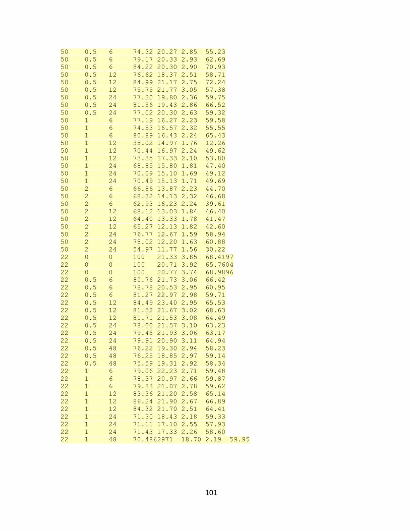
101
50 0.5 6 74.32 20.27 2.85 55.23
50 0.5 6 79.17 20.33 2.93 62.69
50 0.5 6 84.22 20.30 2.90 70.93
50 0.5 12 76.62 18.37 2.51 58.71
50 0.5 12 84.99 21.17 2.75 72.24
50 0.5 12 75.75 21.77 3.05 57.38
50 0.5 24 77.30 19.80 2.36 59.75
50 0.5 24 81.56 19.43 2.86 66.52
50 0.5 24 77.02 20.30 2.63 59.32
50 1 6 77.19 16.27 2.23 59.58
50 1 6 74.53 16.57 2.32 55.55
50 1 6 80.89 16.43 2.24 65.43
50 1 12 35.02 14.97 1.76 12.26
50 1 12 70.44 16.97 2.24 49.62
50 1 12 73.35 17.33 2.10 53.80
50 1 24 68.85 15.80 1.81 47.40
50 1 24 70.09 15.10 1.69 49.12
50 1 24 70.49 15.13 1.71 49.69
50 2 6 66.86 13.87 2.23 44.70
50 2 6 68.32 14.13 2.32 46.68
50 2 6 62.93 16.23 2.24 39.61
50 2 12 68.12 13.03 1.84 46.40
50 2 12 64.40 13.33 1.78 41.47
50 2 12 65.27 12.13 1.82 42.60
50 2 24 76.77 12.67 1.59 58.94
50 2 24 78.02 12.20 1.63 60.88
50 2 24 54.97 11.77 1.56 30.22
22 0 0 100 21.33 3.85 68.4197
22 0 0 100 20.71 3.92 65.7604
22 0 0 100 20.77 3.74 68.9896
22 0.5 6 80.76 21.73 3.06 66.42
22 0.5 6 78.78 20.53 2.95 60.95
22 0.5 6 81.27 22.97 2.98 59.71
22 0.5 12 84.49 23.40 2.95 65.53
22 0.5 12 81.52 21.67 3.02 68.63
22 0.5 12 81.71 21.53 3.08 64.49
22 0.5 24 78.00 21.57 3.10 63.23
22 0.5 24 79.45 21.93 3.06 63.17
22 0.5 24 79.91 20.90 3.11 64.94
22 0.5 48 76.22 19.30 2.94 58.23
22 0.5 48 76.25 18.85 2.97 59.14
22 0.5 48 75.59 19.31 2.92 58.34
22 1 6 79.06 22.23 2.71 59.48
22 1 6 78.37 20.97 2.66 59.87
22 1 6 79.88 21.07 2.78 59.62
22 1 12 83.36 21.20 2.58 65.14
22 1 12 86.24 21.90 2.67 66.89
22 1 12 84.32 21.70 2.51 64.41
22 1 24 71.30 18.43 2.18 59.33
22 1 24 71.11 17.10 2.55 57.93
22 1 24 71.43 17.33 2.26 58.60
22 1 48 70.4862971 18.70 2.19 59.95
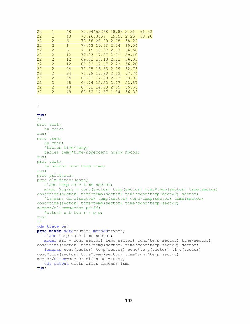
102
22 1 48 72.94462268 18.83 2.31 61.32
22 1 48 71.2683857 19.50 2.25 58.26
22 2 6 73.58 20.90 2.18 58.22
22 2 6 74.42 19.53 2.24 60.04
22 2 6 71.19 18.97 2.07 56.60
22 2 12 72.03 17.27 2.01 59.10
22 2 12 69.81 18.13 2.11 56.05
22 2 12 60.33 17.67 2.23 56.20
22 2 24 77.05 16.53 2.19 62.76
22 2 24 71.39 16.93 2.12 57.74
22 2 24 65.93 17.30 2.13 53.96
22 2 48 64.74 15.33 2.07 52.87
22 2 48 67.52 14.93 2.05 55.66
22 2 48 67.52 14.67 1.84 56.32
;
run;
/*
proc sort;
by conc;
run;
proc freq;
by conc;
*tables time*temp;
tables temp*time/nopercent norow nocol;
run;
proc sort;
by sector conc temp time;
run;
proc print;run;
proc glm data=sugars;
class temp conc time sector;
model Sugars = conc(sector) temp(sector) conc*temp(sector) time(sector)
conc*time(sector) time*temp(sector) time*conc*temp(sector) sector;
*lsmeans conc(sector) temp(sector) conc*temp(sector) time(sector)
conc*time(sector) time*temp(sector) time*conc*temp(sector)
sector/slice=sector pdiff;
*output out=two r=r p=p;
run;
*/
ods trace on;
proc mixed data=sugars method=type3;
class temp conc time sector;
model ail = conc(sector) temp(sector) conc*temp(sector) time(sector)
conc*time(sector) time*temp(sector) time*conc*temp(sector) sector;
lsmeans conc(sector) temp(sector) conc*temp(sector) time(sector)
conc*time(sector) time*temp(sector) time*conc*temp(sector)
sector/slice=sector diffs adj=tukey;
ods output diffs=diffs lsmeans=lsm;
run;
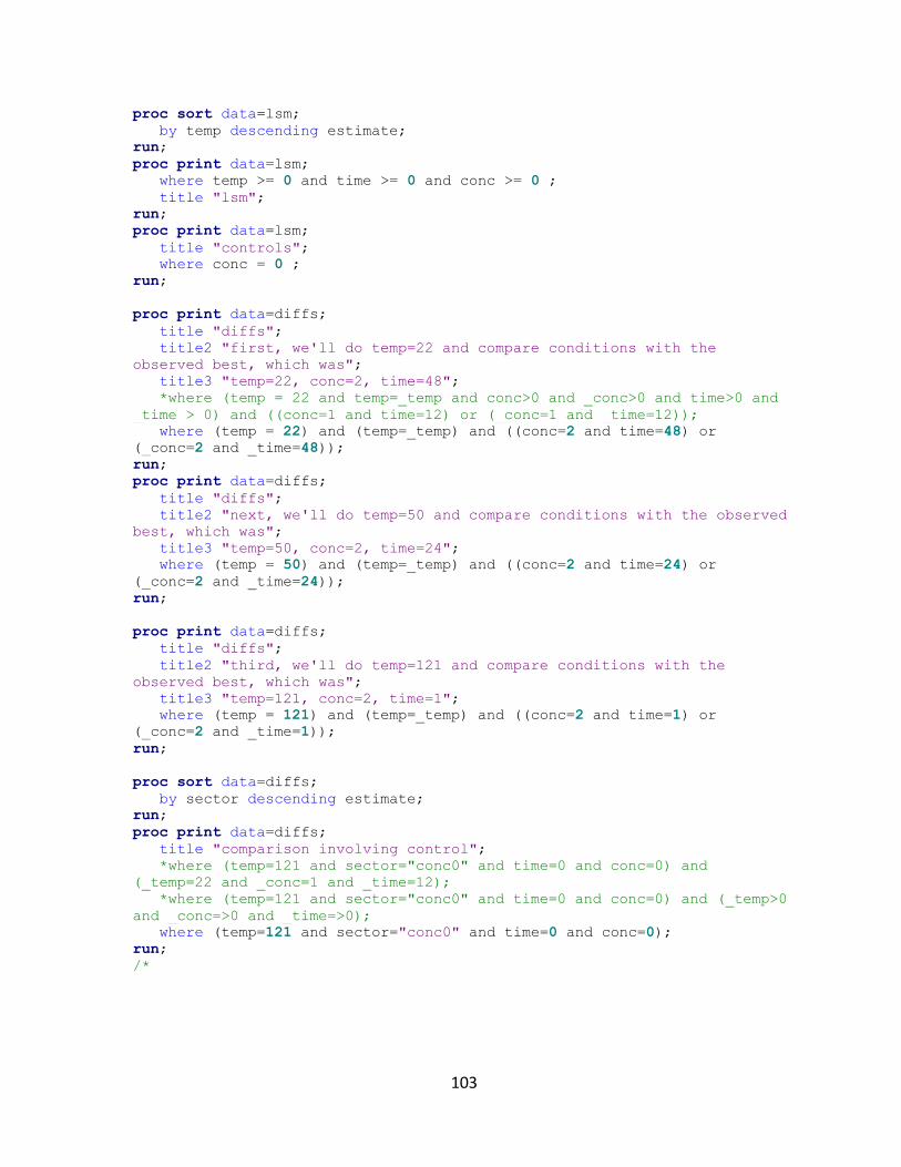
103
proc sort data=lsm;
by temp descending estimate;
run;
proc print data=lsm;
where temp >= 0 and time >= 0 and conc >= 0 ;
title "lsm";
run;
proc print data=lsm;
title "controls";
where conc = 0 ;
run;
proc print data=diffs;
title "diffs";
title2 "first, we'll do temp=22 and compare conditions with the
observed best, which was";
title3 "temp=22, conc=2, time=48";
*where (temp = 22 and temp=_temp and conc>0 and _conc>0 and time>0 and
_time > 0) and ((conc=1 and time=12) or (_conc=1 and _time=12));
where (temp = 22) and (temp=_temp) and ((conc=2 and time=48) or
(_conc=2 and _time=48));
run;
proc print data=diffs;
title "diffs";
title2 "next, we'll do temp=50 and compare conditions with the observed
best, which was";
title3 "temp=50, conc=2, time=24";
where (temp = 50) and (temp=_temp) and ((conc=2 and time=24) or
(_conc=2 and _time=24));
run;
proc print data=diffs;
title "diffs";
title2 "third, we'll do temp=121 and compare conditions with the
observed best, which was";
title3 "temp=121, conc=2, time=1";
where (temp = 121) and (temp=_temp) and ((conc=2 and time=1) or
(_conc=2 and _time=1));
run;
proc sort data=diffs;
by sector descending estimate;
run;
proc print data=diffs;
title "comparison involving control";
*where (temp=121 and sector="conc0" and time=0 and conc=0) and
(_temp=22 and _conc=1 and _time=12);
*where (temp=121 and sector="conc0" and time=0 and conc=0) and (_temp>0
and _conc=>0 and _time=>0);
where (temp=121 and sector="conc0" and time=0 and conc=0);
run;
/*

104
proc print data=diffs;
title "comparison involving control";
where (temp=121 and sector="conc0" and time=0 and conc=0) and (_temp=50
and _conc=.5 and _time=24);
run;
proc print data=diffs;
title "comparison involving control";
where (temp=121 and sector="conc0" and time=0 and conc=0) and
(_temp=121 and _conc=.5 and _time=.5);
run;
*/
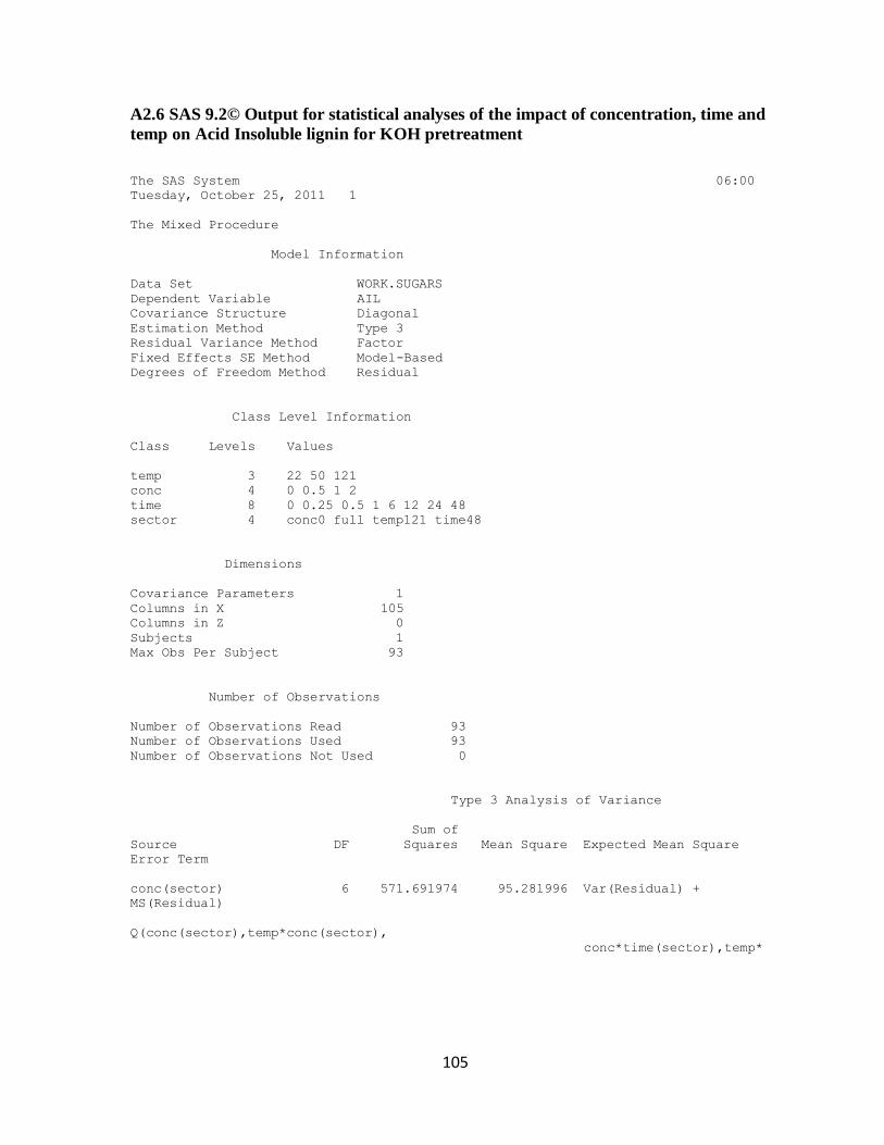
105
A2.6 SAS 9.2© Output for statistical analyses of the impact of concentration, time and
temp on Acid Insoluble lignin for KOH pretreatment
The SAS System 06:00
Tuesday, October 25, 2011 1
The Mixed Procedure
Model Information
Data Set WORK.SUGARS
Dependent Variable AIL
Covariance Structure Diagonal
Estimation Method Type 3
Residual Variance Method Factor
Fixed Effects SE Method Model-Based
Degrees of Freedom Method Residual
Class Level Information
Class Levels Values
temp 3 22 50 121
conc 4 0 0.5 1 2
time 8 0 0.25 0.5 1 6 12 24 48
sector 4 conc0 full temp121 time48
Dimensions
Covariance Parameters 1
Columns in X 105
Columns in Z 0
Subjects 1
Max Obs Per Subject 93
Number of Observations
Number of Observations Read 93
Number of Observations Used 93
Number of Observations Not Used 0
Type 3 Analysis of Variance
Sum of
Source DF Squares Mean Square Expected Mean Square
Error Term
conc(sector) 6 571.691974 95.281996 Var(Residual) +
MS(Residual)
Q(conc(sector),temp*conc(sector),
conc*time(sector),temp*
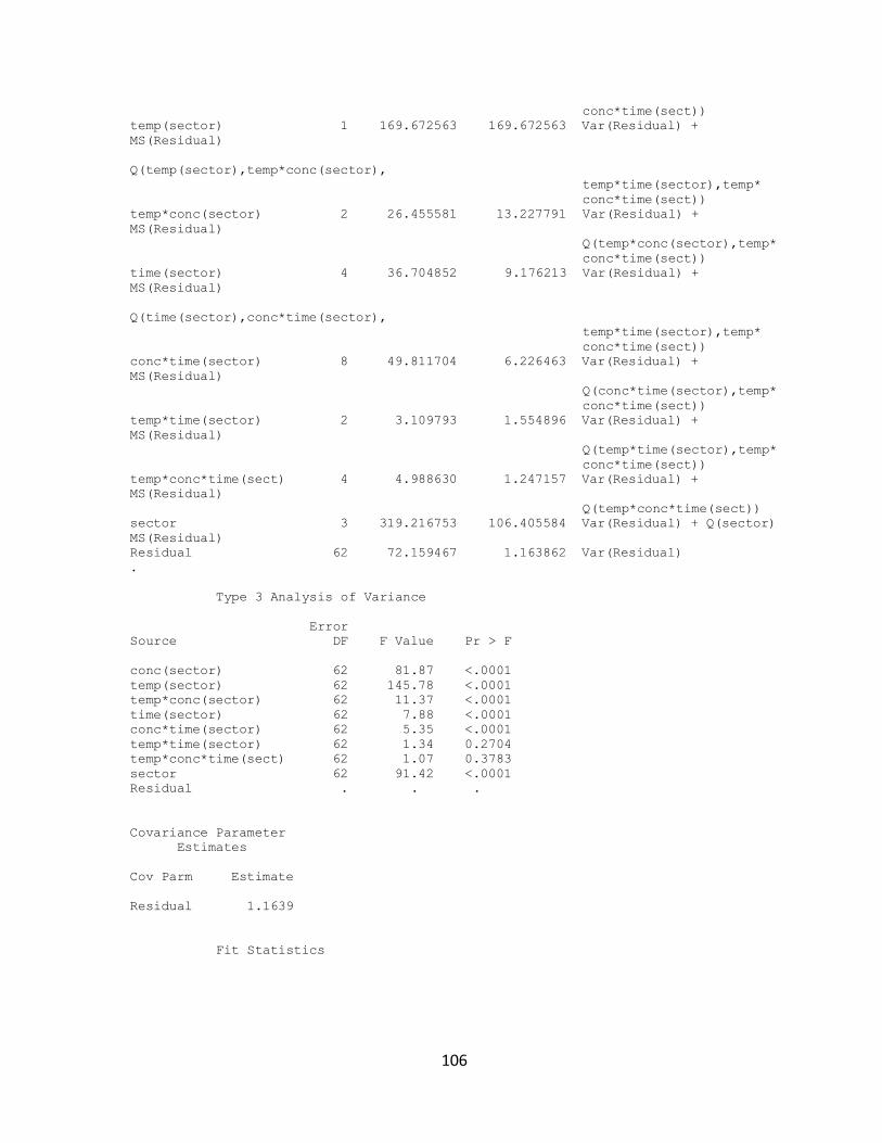
106
conc*time(sect))
temp(sector) 1 169.672563 169.672563 Var(Residual) +
MS(Residual)
Q(temp(sector),temp*conc(sector),
temp*time(sector),temp*
conc*time(sect))
temp*conc(sector) 2 26.455581 13.227791 Var(Residual) +
MS(Residual)
Q(temp*conc(sector),temp*
conc*time(sect))
time(sector) 4 36.704852 9.176213 Var(Residual) +
MS(Residual)
Q(time(sector),conc*time(sector),
temp*time(sector),temp*
conc*time(sect))
conc*time(sector) 8 49.811704 6.226463 Var(Residual) +
MS(Residual)
Q(conc*time(sector),temp*
conc*time(sect))
temp*time(sector) 2 3.109793 1.554896 Var(Residual) +
MS(Residual)
Q(temp*time(sector),temp*
conc*time(sect))
temp*conc*time(sect) 4 4.988630 1.247157 Var(Residual) +
MS(Residual)
Q(temp*conc*time(sect))
sector 3 319.216753 106.405584 Var(Residual) + Q(sector)
MS(Residual)
Residual 62 72.159467 1.163862 Var(Residual)
.
Type 3 Analysis of Variance
Error
Source DF F Value Pr > F
conc(sector) 62 81.87 <.0001
temp(sector) 62 145.78 <.0001
temp*conc(sector) 62 11.37 <.0001
time(sector) 62 7.88 <.0001
conc*time(sector) 62 5.35 <.0001
temp*time(sector) 62 1.34 0.2704
temp*conc*time(sect) 62 1.07 0.3783
sector 62 91.42 <.0001
Residual . . .
Covariance Parameter
Estimates
Cov Parm Estimate
Residual 1.1639
Fit Statistics
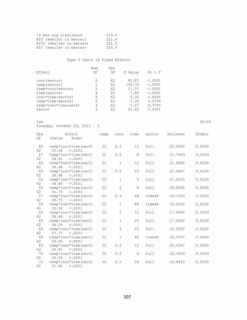
107
-2 Res Log Likelihood 219.4
AIC (smaller is better) 221.4
AICC (smaller is better) 221.5
BIC (smaller is better) 223.5
Type 3 Tests of Fixed Effects
Num Den
Effect DF DF F Value Pr > F
conc(sector) 6 62 81.87 <.0001
temp(sector) 1 62 145.78 <.0001
temp*conc(sector) 2 62 11.37 <.0001
time(sector) 4 62 7.88 <.0001
conc*time(sector) 8 62 5.35 <.0001
temp*time(sector) 2 62 1.34 0.2704
temp*conc*time(sect) 4 62 1.07 0.3783
sector 3 62 91.42 <.0001
lsm 06:00
Tuesday, October 25, 2011 5
Obs Effect temp conc time sector Estimate StdErr
DF tValue Probt
45 temp*conc*time(sect) 22 0.5 12 full 22.2000 0.6229
62 35.64 <.0001
47 temp*conc*time(sect) 22 0.5 6 full 21.7433 0.6229
62 34.91 <.0001
48 temp*conc*time(sect) 22 1 12 full 21.6000 0.6229
62 34.68 <.0001
49 temp*conc*time(sect) 22 0.5 24 full 21.4667 0.6229
62 34.46 <.0001
50 temp*conc*time(sect) 22 1 6 full 21.4233 0.6229
62 34.40 <.0001
55 temp*conc*time(sect) 22 2 6 full 19.8000 0.6229
62 31.79 <.0001
57 temp*conc*time(sect) 22 0.5 48 time48 19.1533 0.6229
62 30.75 <.0001
59 temp*conc*time(sect) 22 1 48 time48 19.0100 0.6229
62 30.52 <.0001
64 temp*conc*time(sect) 22 2 12 full 17.6900 0.6229
62 28.40 <.0001
65 temp*conc*time(sect) 22 1 24 full 17.6200 0.6229
62 28.29 <.0001
66 temp*conc*time(sect) 22 2 24 full 16.9200 0.6229
62 27.17 <.0001
68 temp*conc*time(sect) 22 2 48 time48 14.9767 0.6229
62 24.05 <.0001
69 temp*conc*time(sect) 50 0.5 12 full 20.4367 0.6229
62 32.81 <.0001
70 temp*conc*time(sect) 50 0.5 6 full 20.3000 0.6229
62 32.59 <.0001
72 temp*conc*time(sect) 50 0.5 24 full 19.8433 0.6229
62 31.86 <.0001
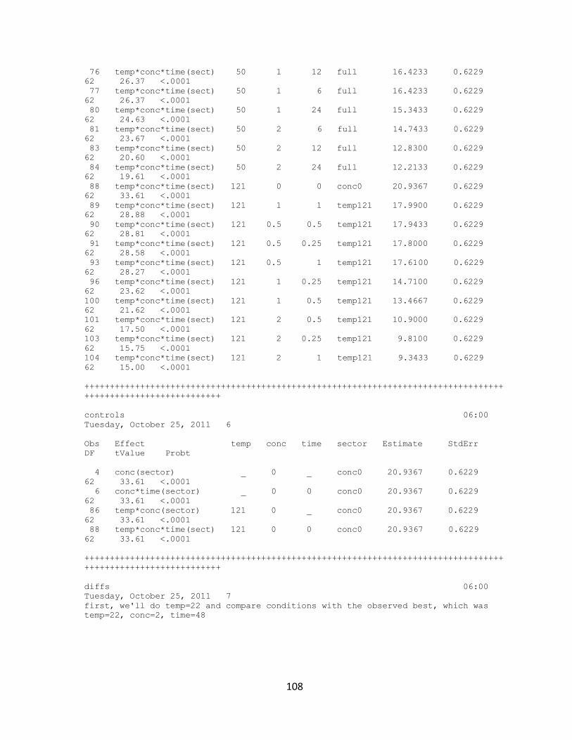
108
76 temp*conc*time(sect) 50 1 12 full 16.4233 0.6229
62 26.37 <.0001
77 temp*conc*time(sect) 50 1 6 full 16.4233 0.6229
62 26.37 <.0001
80 temp*conc*time(sect) 50 1 24 full 15.3433 0.6229
62 24.63 <.0001
81 temp*conc*time(sect) 50 2 6 full 14.7433 0.6229
62 23.67 <.0001
83 temp*conc*time(sect) 50 2 12 full 12.8300 0.6229
62 20.60 <.0001
84 temp*conc*time(sect) 50 2 24 full 12.2133 0.6229
62 19.61 <.0001
88 temp*conc*time(sect) 121 0 0 conc0 20.9367 0.6229
62 33.61 <.0001
89 temp*conc*time(sect) 121 1 1 temp121 17.9900 0.6229
62 28.88 <.0001
90 temp*conc*time(sect) 121 0.5 0.5 temp121 17.9433 0.6229
62 28.81 <.0001
91 temp*conc*time(sect) 121 0.5 0.25 temp121 17.8000 0.6229
62 28.58 <.0001
93 temp*conc*time(sect) 121 0.5 1 temp121 17.6100 0.6229
62 28.27 <.0001
96 temp*conc*time(sect) 121 1 0.25 temp121 14.7100 0.6229
62 23.62 <.0001
100 temp*conc*time(sect) 121 1 0.5 temp121 13.4667 0.6229
62 21.62 <.0001
101 temp*conc*time(sect) 121 2 0.5 temp121 10.9000 0.6229
62 17.50 <.0001
103 temp*conc*time(sect) 121 2 0.25 temp121 9.8100 0.6229
62 15.75 <.0001
104 temp*conc*time(sect) 121 2 1 temp121 9.3433 0.6229
62 15.00 <.0001
+++++++++++++++++++++++++++++++++++++++++++++++++++++++++++++++++++++++++++++++++++
+++++++++++++++++++++++++++
controls 06:00
Tuesday, October 25, 2011 6
Obs Effect temp conc time sector Estimate StdErr
DF tValue Probt
4 conc(sector) _ 0 _ conc0 20.9367 0.6229
62 33.61 <.0001
6 conc*time(sector) _ 0 0 conc0 20.9367 0.6229
62 33.61 <.0001
86 temp*conc(sector) 121 0 _ conc0 20.9367 0.6229
62 33.61 <.0001
88 temp*conc*time(sect) 121 0 0 conc0 20.9367 0.6229
62 33.61 <.0001
+++++++++++++++++++++++++++++++++++++++++++++++++++++++++++++++++++++++++++++++++++
+++++++++++++++++++++++++++
diffs 06:00
Tuesday, October 25, 2011 7
first, we'll do temp=22 and compare conditions with the observed best, which was
temp=22, conc=2, time=48
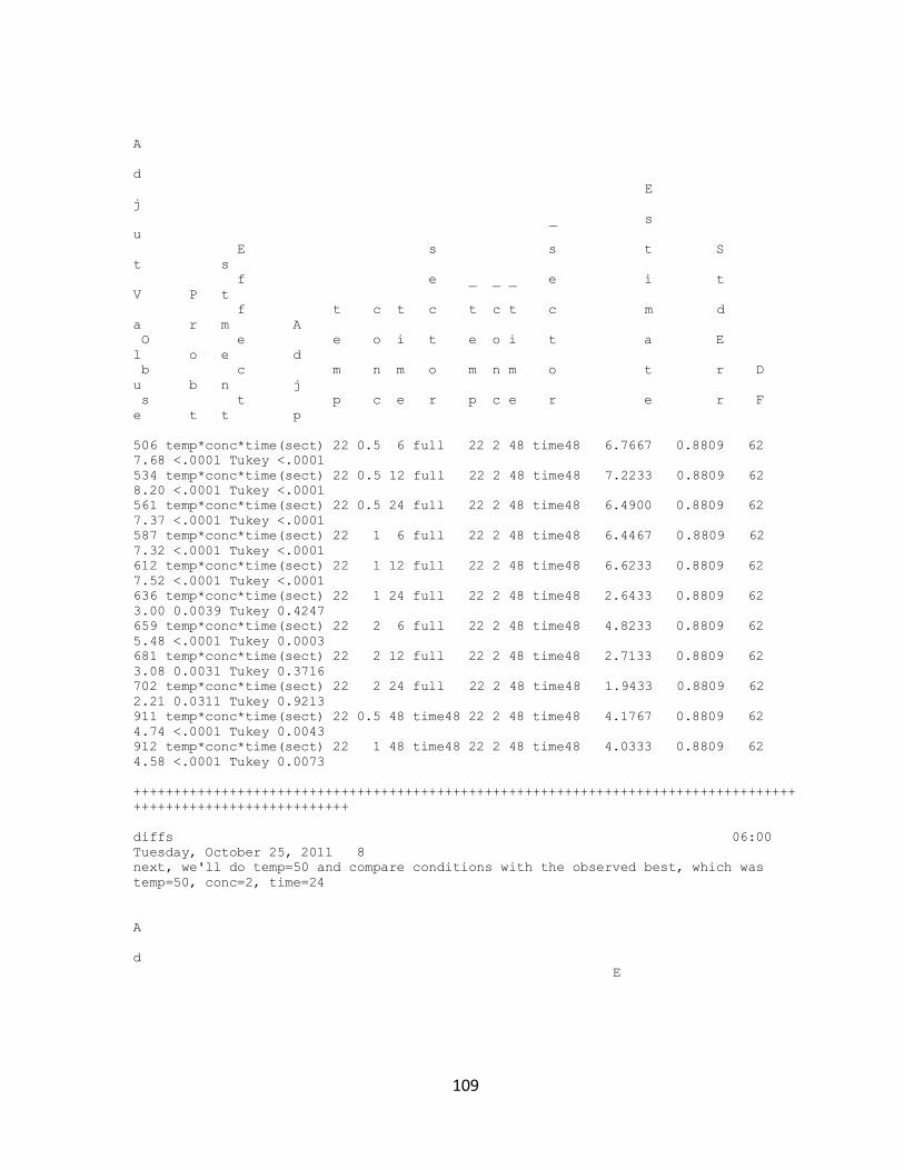
109
A
d
E
j
_ s
u
E s s t S
t s
f e _ _ _ e i t
V P t
f t c t c t c t c m d
a r m A
O e e o i t e o i t a E
l o e d
b c m n m o m n m o t r D
u b n j
s t p c e r p c e r e r F
e t t p
506 temp*conc*time(sect) 22 0.5 6 full 22 2 48 time48 6.7667 0.8809 62
7.68 <.0001 Tukey <.0001
534 temp*conc*time(sect) 22 0.5 12 full 22 2 48 time48 7.2233 0.8809 62
8.20 <.0001 Tukey <.0001
561 temp*conc*time(sect) 22 0.5 24 full 22 2 48 time48 6.4900 0.8809 62
7.37 <.0001 Tukey <.0001
587 temp*conc*time(sect) 22 1 6 full 22 2 48 time48 6.4467 0.8809 62
7.32 <.0001 Tukey <.0001
612 temp*conc*time(sect) 22 1 12 full 22 2 48 time48 6.6233 0.8809 62
7.52 <.0001 Tukey <.0001
636 temp*conc*time(sect) 22 1 24 full 22 2 48 time48 2.6433 0.8809 62
3.00 0.0039 Tukey 0.4247
659 temp*conc*time(sect) 22 2 6 full 22 2 48 time48 4.8233 0.8809 62
5.48 <.0001 Tukey 0.0003
681 temp*conc*time(sect) 22 2 12 full 22 2 48 time48 2.7133 0.8809 62
3.08 0.0031 Tukey 0.3716
702 temp*conc*time(sect) 22 2 24 full 22 2 48 time48 1.9433 0.8809 62
2.21 0.0311 Tukey 0.9213
911 temp*conc*time(sect) 22 0.5 48 time48 22 2 48 time48 4.1767 0.8809 62
4.74 <.0001 Tukey 0.0043
912 temp*conc*time(sect) 22 1 48 time48 22 2 48 time48 4.0333 0.8809 62
4.58 <.0001 Tukey 0.0073
+++++++++++++++++++++++++++++++++++++++++++++++++++++++++++++++++++++++++++++++++++
+++++++++++++++++++++++++++
diffs 06:00
Tuesday, October 25, 2011 8
next, we'll do temp=50 and compare conditions with the observed best, which was
temp=50, conc=2, time=24
A
d
E
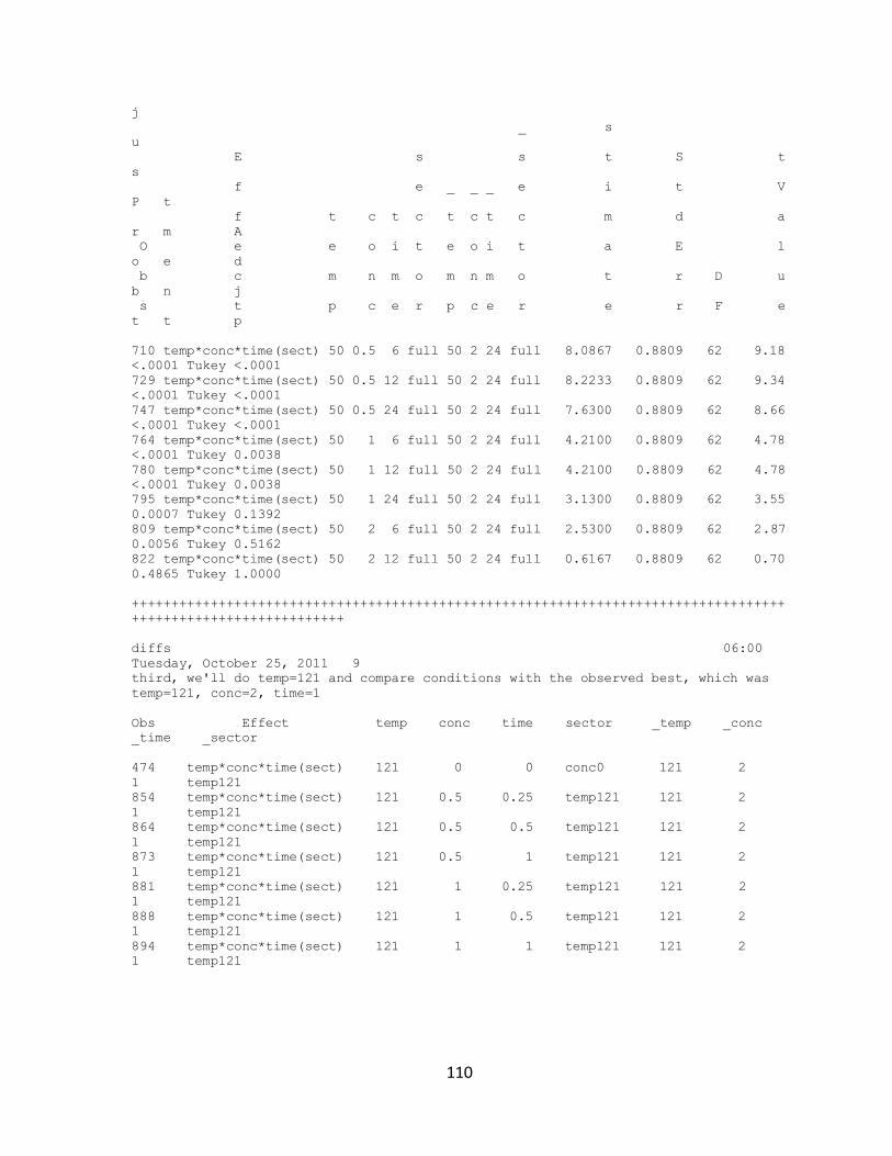
110
j
_ s
u
E s s t S t
s
f e _ _ _ e i t V
P t
f t c t c t c t c m d a
r m A
O e e o i t e o i t a E l
o e d
b c m n m o m n m o t r D u
b n j
s t p c e r p c e r e r F e
t t p
710 temp*conc*time(sect) 50 0.5 6 full 50 2 24 full 8.0867 0.8809 62 9.18
<.0001 Tukey <.0001
729 temp*conc*time(sect) 50 0.5 12 full 50 2 24 full 8.2233 0.8809 62 9.34
<.0001 Tukey <.0001
747 temp*conc*time(sect) 50 0.5 24 full 50 2 24 full 7.6300 0.8809 62 8.66
<.0001 Tukey <.0001
764 temp*conc*time(sect) 50 1 6 full 50 2 24 full 4.2100 0.8809 62 4.78
<.0001 Tukey 0.0038
780 temp*conc*time(sect) 50 1 12 full 50 2 24 full 4.2100 0.8809 62 4.78
<.0001 Tukey 0.0038
795 temp*conc*time(sect) 50 1 24 full 50 2 24 full 3.1300 0.8809 62 3.55
0.0007 Tukey 0.1392
809 temp*conc*time(sect) 50 2 6 full 50 2 24 full 2.5300 0.8809 62 2.87
0.0056 Tukey 0.5162
822 temp*conc*time(sect) 50 2 12 full 50 2 24 full 0.6167 0.8809 62 0.70
0.4865 Tukey 1.0000
+++++++++++++++++++++++++++++++++++++++++++++++++++++++++++++++++++++++++++++++++++
+++++++++++++++++++++++++++
diffs 06:00
Tuesday, October 25, 2011 9
third, we'll do temp=121 and compare conditions with the observed best, which was
temp=121, conc=2, time=1
Obs Effect temp conc time sector _temp _conc
_time _sector
474 temp*conc*time(sect) 121 0 0 conc0 121 2
1 temp121
854 temp*conc*time(sect) 121 0.5 0.25 temp121 121 2
1 temp121
864 temp*conc*time(sect) 121 0.5 0.5 temp121 121 2
1 temp121
873 temp*conc*time(sect) 121 0.5 1 temp121 121 2
1 temp121
881 temp*conc*time(sect) 121 1 0.25 temp121 121 2
1 temp121
888 temp*conc*time(sect) 121 1 0.5 temp121 121 2
1 temp121
894 temp*conc*time(sect) 121 1 1 temp121 121 2
1 temp121
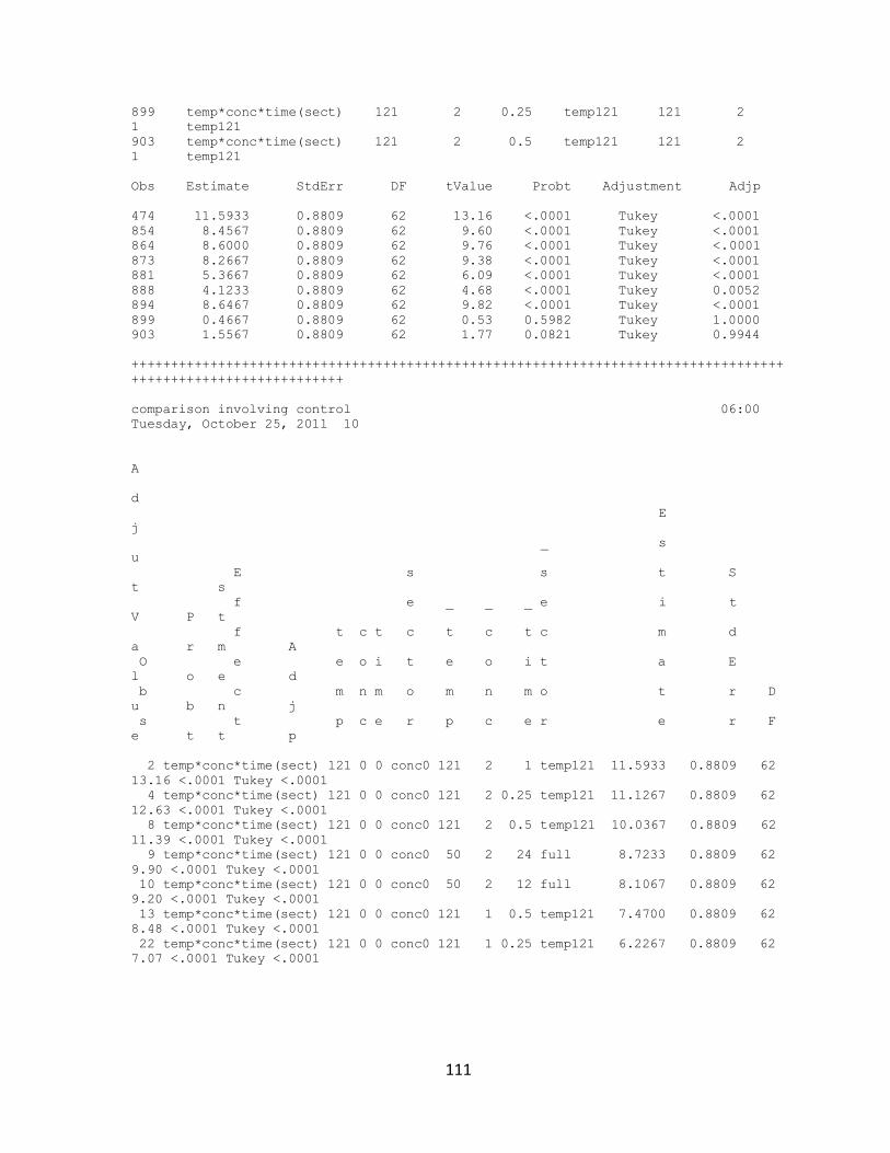
111
899 temp*conc*time(sect) 121 2 0.25 temp121 121 2
1 temp121
903 temp*conc*time(sect) 121 2 0.5 temp121 121 2
1 temp121
Obs Estimate StdErr DF tValue Probt Adjustment Adjp
474 11.5933 0.8809 62 13.16 <.0001 Tukey <.0001
854 8.4567 0.8809 62 9.60 <.0001 Tukey <.0001
864 8.6000 0.8809 62 9.76 <.0001 Tukey <.0001
873 8.2667 0.8809 62 9.38 <.0001 Tukey <.0001
881 5.3667 0.8809 62 6.09 <.0001 Tukey <.0001
888 4.1233 0.8809 62 4.68 <.0001 Tukey 0.0052
894 8.6467 0.8809 62 9.82 <.0001 Tukey <.0001
899 0.4667 0.8809 62 0.53 0.5982 Tukey 1.0000
903 1.5567 0.8809 62 1.77 0.0821 Tukey 0.9944
+++++++++++++++++++++++++++++++++++++++++++++++++++++++++++++++++++++++++++++++++++
+++++++++++++++++++++++++++
comparison involving control 06:00
Tuesday, October 25, 2011 10
A
d
E
j
_ s
u
E s s t S
t s
f e _ _ _ e i t
V P t
f t c t c t c t c m d
a r m A
O e e o i t e o i t a E
l o e d
b c m n m o m n m o t r D
u b n j
s t p c e r p c e r e r F
e t t p
2 temp*conc*time(sect) 121 0 0 conc0 121 2 1 temp121 11.5933 0.8809 62
13.16 <.0001 Tukey <.0001
4 temp*conc*time(sect) 121 0 0 conc0 121 2 0.25 temp121 11.1267 0.8809 62
12.63 <.0001 Tukey <.0001
8 temp*conc*time(sect) 121 0 0 conc0 121 2 0.5 temp121 10.0367 0.8809 62
11.39 <.0001 Tukey <.0001
9 temp*conc*time(sect) 121 0 0 conc0 50 2 24 full 8.7233 0.8809 62
9.90 <.0001 Tukey <.0001
10 temp*conc*time(sect) 121 0 0 conc0 50 2 12 full 8.1067 0.8809 62
9.20 <.0001 Tukey <.0001
13 temp*conc*time(sect) 121 0 0 conc0 121 1 0.5 temp121 7.4700 0.8809 62
8.48 <.0001 Tukey <.0001
22 temp*conc*time(sect) 121 0 0 conc0 121 1 0.25 temp121 6.2267 0.8809 62
7.07 <.0001 Tukey <.0001
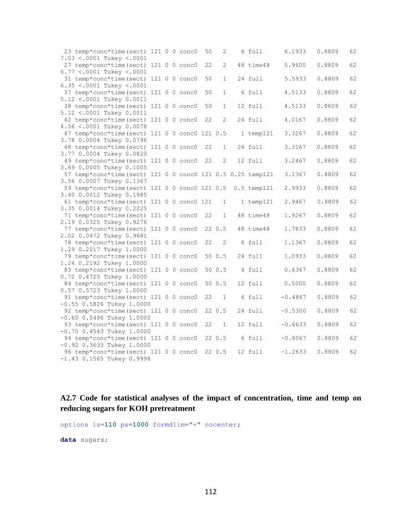
112
23 temp*conc*time(sect) 121 0 0 conc0 50 2 6 full 6.1933 0.8809 62
7.03 <.0001 Tukey <.0001
27 temp*conc*time(sect) 121 0 0 conc0 22 2 48 time48 5.9600 0.8809 62
6.77 <.0001 Tukey <.0001
31 temp*conc*time(sect) 121 0 0 conc0 50 1 24 full 5.5933 0.8809 62
6.35 <.0001 Tukey <.0001
37 temp*conc*time(sect) 121 0 0 conc0 50 1 6 full 4.5133 0.8809 62
5.12 <.0001 Tukey 0.0011
38 temp*conc*time(sect) 121 0 0 conc0 50 1 12 full 4.5133 0.8809 62
5.12 <.0001 Tukey 0.0011
42 temp*conc*time(sect) 121 0 0 conc0 22 2 24 full 4.0167 0.8809 62
4.56 <.0001 Tukey 0.0078
47 temp*conc*time(sect) 121 0 0 conc0 121 0.5 1 temp121 3.3267 0.8809 62
3.78 0.0004 Tukey 0.0796
48 temp*conc*time(sect) 121 0 0 conc0 22 1 24 full 3.3167 0.8809 62
3.77 0.0004 Tukey 0.0820
49 temp*conc*time(sect) 121 0 0 conc0 22 2 12 full 3.2467 0.8809 62
3.69 0.0005 Tukey 0.1005
57 temp*conc*time(sect) 121 0 0 conc0 121 0.5 0.25 temp121 3.1367 0.8809 62
3.56 0.0007 Tukey 0.1367
59 temp*conc*time(sect) 121 0 0 conc0 121 0.5 0.5 temp121 2.9933 0.8809 62
3.40 0.0012 Tukey 0.1985
61 temp*conc*time(sect) 121 0 0 conc0 121 1 1 temp121 2.9467 0.8809 62
3.35 0.0014 Tukey 0.2225
71 temp*conc*time(sect) 121 0 0 conc0 22 1 48 time48 1.9267 0.8809 62
2.19 0.0325 Tukey 0.9276
77 temp*conc*time(sect) 121 0 0 conc0 22 0.5 48 time48 1.7833 0.8809 62
2.02 0.0472 Tukey 0.9681
78 temp*conc*time(sect) 121 0 0 conc0 22 2 6 full 1.1367 0.8809 62
1.29 0.2017 Tukey 1.0000
79 temp*conc*time(sect) 121 0 0 conc0 50 0.5 24 full 1.0933 0.8809 62
1.24 0.2192 Tukey 1.0000
83 temp*conc*time(sect) 121 0 0 conc0 50 0.5 6 full 0.6367 0.8809 62
0.72 0.4725 Tukey 1.0000
84 temp*conc*time(sect) 121 0 0 conc0 50 0.5 12 full 0.5000 0.8809 62
0.57 0.5723 Tukey 1.0000
91 temp*conc*time(sect) 121 0 0 conc0 22 1 6 full -0.4867 0.8809 62
-0.55 0.5826 Tukey 1.0000
92 temp*conc*time(sect) 121 0 0 conc0 22 0.5 24 full -0.5300 0.8809 62
-0.60 0.5496 Tukey 1.0000
93 temp*conc*time(sect) 121 0 0 conc0 22 1 12 full -0.6633 0.8809 62
-0.75 0.4543 Tukey 1.0000
94 temp*conc*time(sect) 121 0 0 conc0 22 0.5 6 full -0.8067 0.8809 62
-0.92 0.3633 Tukey 1.0000
96 temp*conc*time(sect) 121 0 0 conc0 22 0.5 12 full -1.2633 0.8809 62
-1.43 0.1565 Tukey 0.9998
A2.7 Code for statistical analyses of the impact of concentration, time and temp on
reducing sugars for KOH pretreatment
options ls=110 ps=1000 formdlim="+" nocenter;
data sugars;
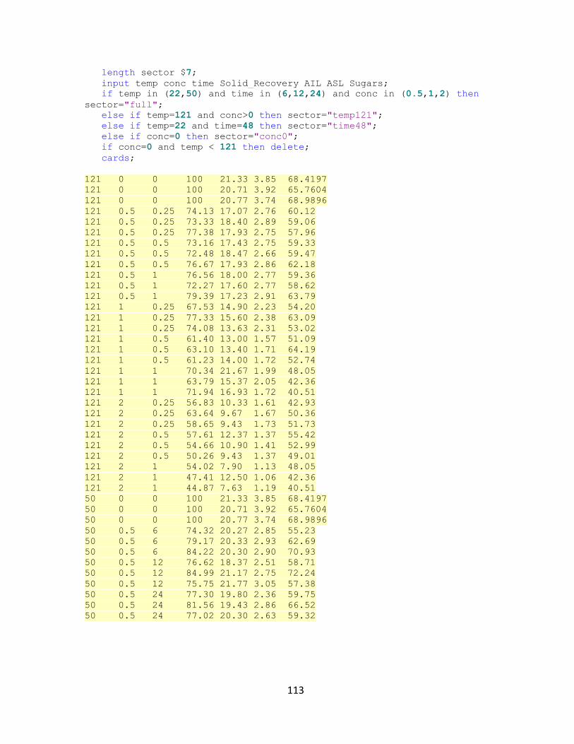
113
length sector $7;
input temp conc time Solid_Recovery AIL ASL Sugars;
if temp in (22,50) and time in (6,12,24) and conc in (0.5,1,2) then
sector="full";
else if temp=121 and conc>0 then sector="temp121";
else if temp=22 and time=48 then sector="time48";
else if conc=0 then sector="conc0";
if conc=0 and temp < 121 then delete;
cards;
121 0 0 100 21.33 3.85 68.4197
121 0 0 100 20.71 3.92 65.7604
121 0 0 100 20.77 3.74 68.9896
121 0.5 0.25 74.13 17.07 2.76 60.12
121 0.5 0.25 73.33 18.40 2.89 59.06
121 0.5 0.25 77.38 17.93 2.75 57.96
121 0.5 0.5 73.16 17.43 2.75 59.33
121 0.5 0.5 72.48 18.47 2.66 59.47
121 0.5 0.5 76.67 17.93 2.86 62.18
121 0.5 1 76.56 18.00 2.77 59.36
121 0.5 1 72.27 17.60 2.77 58.62
121 0.5 1 79.39 17.23 2.91 63.79
121 1 0.25 67.53 14.90 2.23 54.20
121 1 0.25 77.33 15.60 2.38 63.09
121 1 0.25 74.08 13.63 2.31 53.02
121 1 0.5 61.40 13.00 1.57 51.09
121 1 0.5 63.10 13.40 1.71 64.19
121 1 0.5 61.23 14.00 1.72 52.74
121 1 1 70.34 21.67 1.99 48.05
121 1 1 63.79 15.37 2.05 42.36
121 1 1 71.94 16.93 1.72 40.51
121 2 0.25 56.83 10.33 1.61 42.93
121 2 0.25 63.64 9.67 1.67 50.36
121 2 0.25 58.65 9.43 1.73 51.73
121 2 0.5 57.61 12.37 1.37 55.42
121 2 0.5 54.66 10.90 1.41 52.99
121 2 0.5 50.26 9.43 1.37 49.01
121 2 1 54.02 7.90 1.13 48.05
121 2 1 47.41 12.50 1.06 42.36
121 2 1 44.87 7.63 1.19 40.51
50 0 0 100 21.33 3.85 68.4197
50 0 0 100 20.71 3.92 65.7604
50 0 0 100 20.77 3.74 68.9896
50 0.5 6 74.32 20.27 2.85 55.23
50 0.5 6 79.17 20.33 2.93 62.69
50 0.5 6 84.22 20.30 2.90 70.93
50 0.5 12 76.62 18.37 2.51 58.71
50 0.5 12 84.99 21.17 2.75 72.24
50 0.5 12 75.75 21.77 3.05 57.38
50 0.5 24 77.30 19.80 2.36 59.75
50 0.5 24 81.56 19.43 2.86 66.52
50 0.5 24 77.02 20.30 2.63 59.32
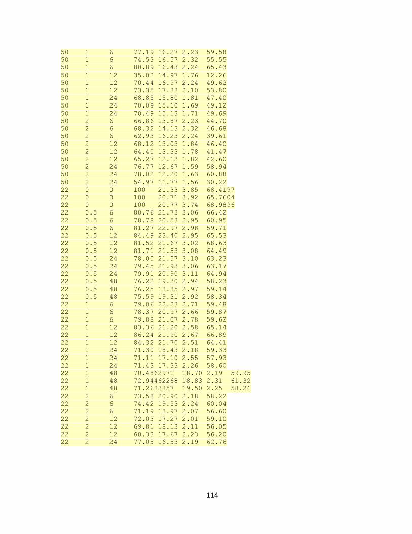
114
50 1 6 77.19 16.27 2.23 59.58
50 1 6 74.53 16.57 2.32 55.55
50 1 6 80.89 16.43 2.24 65.43
50 1 12 35.02 14.97 1.76 12.26
50 1 12 70.44 16.97 2.24 49.62
50 1 12 73.35 17.33 2.10 53.80
50 1 24 68.85 15.80 1.81 47.40
50 1 24 70.09 15.10 1.69 49.12
50 1 24 70.49 15.13 1.71 49.69
50 2 6 66.86 13.87 2.23 44.70
50 2 6 68.32 14.13 2.32 46.68
50 2 6 62.93 16.23 2.24 39.61
50 2 12 68.12 13.03 1.84 46.40
50 2 12 64.40 13.33 1.78 41.47
50 2 12 65.27 12.13 1.82 42.60
50 2 24 76.77 12.67 1.59 58.94
50 2 24 78.02 12.20 1.63 60.88
50 2 24 54.97 11.77 1.56 30.22
22 0 0 100 21.33 3.85 68.4197
22 0 0 100 20.71 3.92 65.7604
22 0 0 100 20.77 3.74 68.9896
22 0.5 6 80.76 21.73 3.06 66.42
22 0.5 6 78.78 20.53 2.95 60.95
22 0.5 6 81.27 22.97 2.98 59.71
22 0.5 12 84.49 23.40 2.95 65.53
22 0.5 12 81.52 21.67 3.02 68.63
22 0.5 12 81.71 21.53 3.08 64.49
22 0.5 24 78.00 21.57 3.10 63.23
22 0.5 24 79.45 21.93 3.06 63.17
22 0.5 24 79.91 20.90 3.11 64.94
22 0.5 48 76.22 19.30 2.94 58.23
22 0.5 48 76.25 18.85 2.97 59.14
22 0.5 48 75.59 19.31 2.92 58.34
22 1 6 79.06 22.23 2.71 59.48
22 1 6 78.37 20.97 2.66 59.87
22 1 6 79.88 21.07 2.78 59.62
22 1 12 83.36 21.20 2.58 65.14
22 1 12 86.24 21.90 2.67 66.89
22 1 12 84.32 21.70 2.51 64.41
22 1 24 71.30 18.43 2.18 59.33
22 1 24 71.11 17.10 2.55 57.93
22 1 24 71.43 17.33 2.26 58.60
22 1 48 70.4862971 18.70 2.19 59.95
22 1 48 72.94462268 18.83 2.31 61.32
22 1 48 71.2683857 19.50 2.25 58.26
22 2 6 73.58 20.90 2.18 58.22
22 2 6 74.42 19.53 2.24 60.04
22 2 6 71.19 18.97 2.07 56.60
22 2 12 72.03 17.27 2.01 59.10
22 2 12 69.81 18.13 2.11 56.05
22 2 12 60.33 17.67 2.23 56.20
22 2 24 77.05 16.53 2.19 62.76
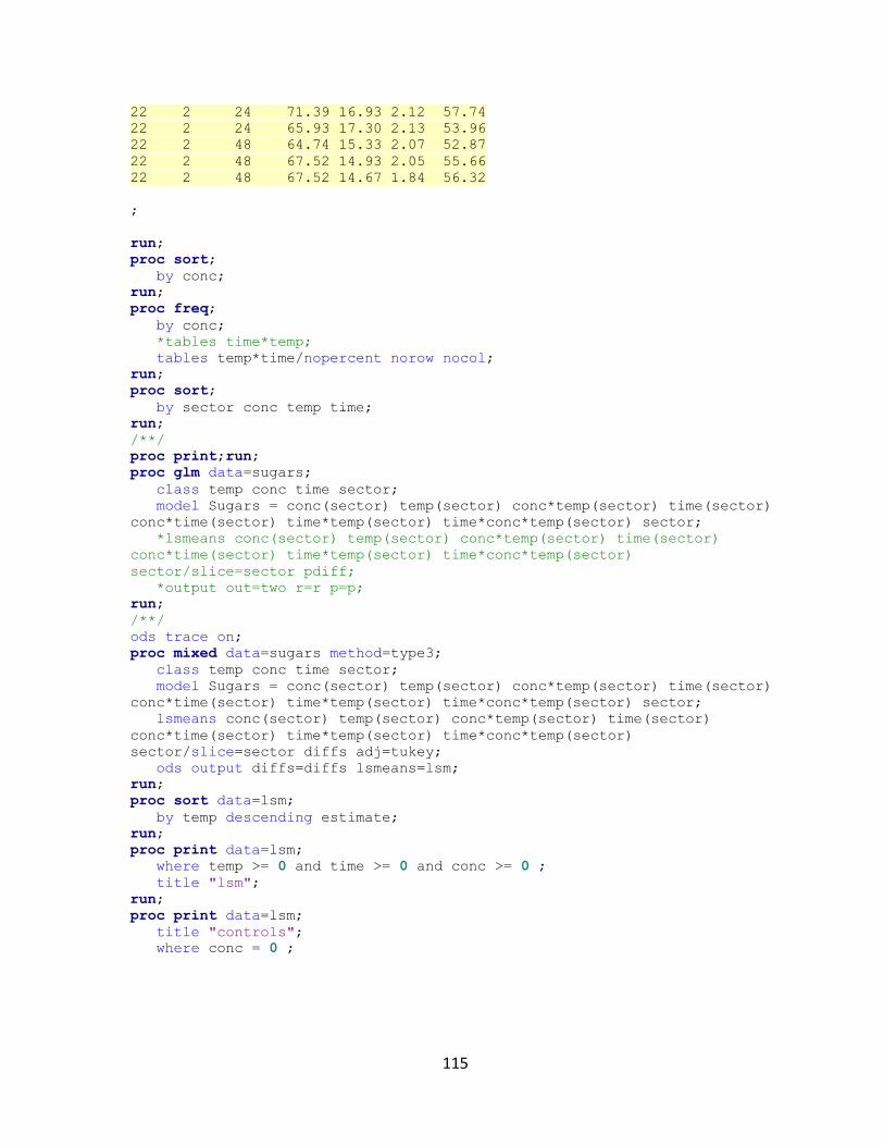
115
22 2 24 71.39 16.93 2.12 57.74
22 2 24 65.93 17.30 2.13 53.96
22 2 48 64.74 15.33 2.07 52.87
22 2 48 67.52 14.93 2.05 55.66
22 2 48 67.52 14.67 1.84 56.32
;
run;
proc sort;
by conc;
run;
proc freq;
by conc;
*tables time*temp;
tables temp*time/nopercent norow nocol;
run;
proc sort;
by sector conc temp time;
run;
/**/
proc print;run;
proc glm data=sugars;
class temp conc time sector;
model Sugars = conc(sector) temp(sector) conc*temp(sector) time(sector)
conc*time(sector) time*temp(sector) time*conc*temp(sector) sector;
*lsmeans conc(sector) temp(sector) conc*temp(sector) time(sector)
conc*time(sector) time*temp(sector) time*conc*temp(sector)
sector/slice=sector pdiff;
*output out=two r=r p=p;
run;
/**/
ods trace on;
proc mixed data=sugars method=type3;
class temp conc time sector;
model Sugars = conc(sector) temp(sector) conc*temp(sector) time(sector)
conc*time(sector) time*temp(sector) time*conc*temp(sector) sector;
lsmeans conc(sector) temp(sector) conc*temp(sector) time(sector)
conc*time(sector) time*temp(sector) time*conc*temp(sector)
sector/slice=sector diffs adj=tukey;
ods output diffs=diffs lsmeans=lsm;
run;
proc sort data=lsm;
by temp descending estimate;
run;
proc print data=lsm;
where temp >= 0 and time >= 0 and conc >= 0 ;
title "lsm";
run;
proc print data=lsm;
title "controls";
where conc = 0 ;
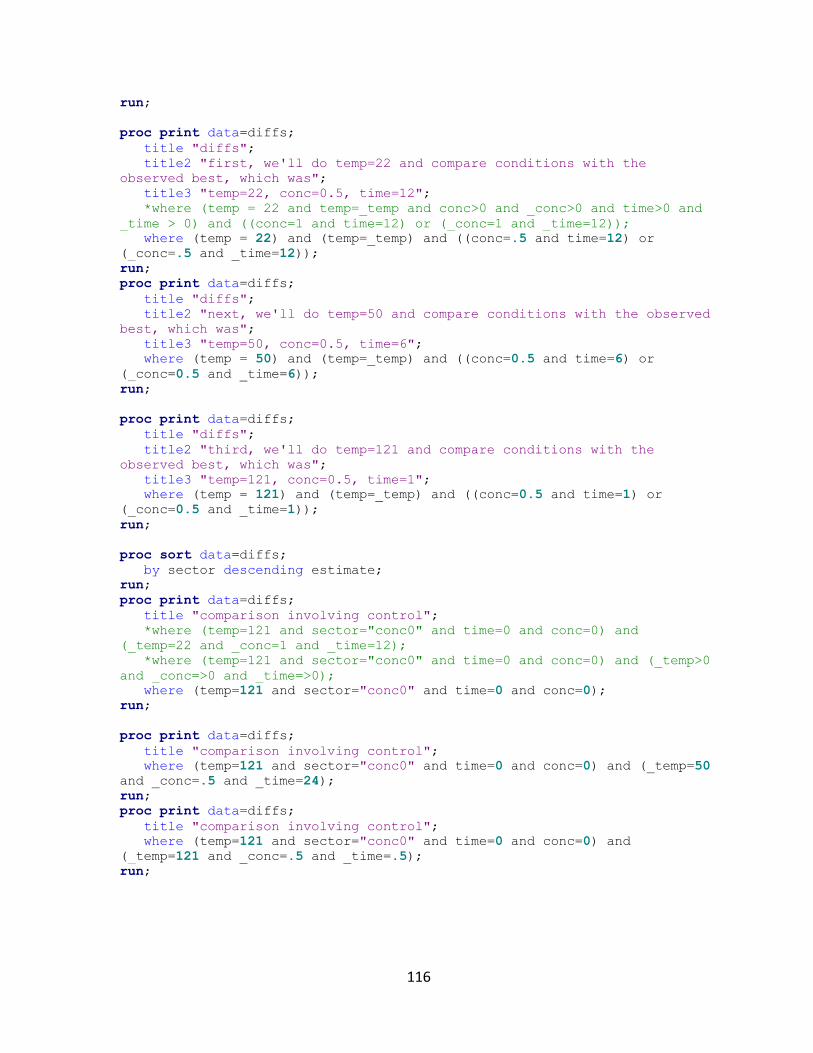
116
run;
proc print data=diffs;
title "diffs";
title2 "first, we'll do temp=22 and compare conditions with the
observed best, which was";
title3 "temp=22, conc=0.5, time=12";
*where (temp = 22 and temp=_temp and conc>0 and _conc>0 and time>0 and
_time > 0) and ((conc=1 and time=12) or (_conc=1 and _time=12));
where (temp = 22) and (temp=_temp) and ((conc=.5 and time=12) or
(_conc=.5 and _time=12));
run;
proc print data=diffs;
title "diffs";
title2 "next, we'll do temp=50 and compare conditions with the observed
best, which was";
title3 "temp=50, conc=0.5, time=6";
where (temp = 50) and (temp=_temp) and ((conc=0.5 and time=6) or
(_conc=0.5 and _time=6));
run;
proc print data=diffs;
title "diffs";
title2 "third, we'll do temp=121 and compare conditions with the
observed best, which was";
title3 "temp=121, conc=0.5, time=1";
where (temp = 121) and (temp=_temp) and ((conc=0.5 and time=1) or
(_conc=0.5 and _time=1));
run;
proc sort data=diffs;
by sector descending estimate;
run;
proc print data=diffs;
title "comparison involving control";
*where (temp=121 and sector="conc0" and time=0 and conc=0) and
(_temp=22 and _conc=1 and _time=12);
*where (temp=121 and sector="conc0" and time=0 and conc=0) and (_temp>0
and _conc=>0 and _time=>0);
where (temp=121 and sector="conc0" and time=0 and conc=0);
run;
proc print data=diffs;
title "comparison involving control";
where (temp=121 and sector="conc0" and time=0 and conc=0) and (_temp=50
and _conc=.5 and _time=24);
run;
proc print data=diffs;
title "comparison involving control";
where (temp=121 and sector="conc0" and time=0 and conc=0) and
(_temp=121 and _conc=.5 and _time=.5);
run;
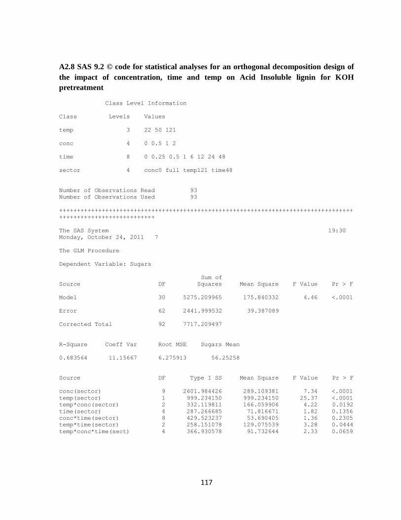
117
A2.8 SAS 9.2 © code for statistical analyses for an orthogonal decomposition design of
the impact of concentration, time and temp on Acid Insoluble lignin for KOH
pretreatment
Class Level Information
Class Levels Values
temp 3 22 50 121
conc 4 0 0.5 1 2
time 8 0 0.25 0.5 1 6 12 24 48
sector 4 conc0 full temp121 time48
Number of Observations Read 93
Number of Observations Used 93
+++++++++++++++++++++++++++++++++++++++++++++++++++++++++++++++++++++++++++++++++++
+++++++++++++++++++++++++++
The SAS System 19:30
Monday, October 24, 2011 7
The GLM Procedure
Dependent Variable: Sugars
Sum of
Source DF Squares Mean Square F Value Pr > F
Model 30 5275.209965 175.840332 4.46 <.0001
Error 62 2441.999532 39.387089
Corrected Total 92 7717.209497
R-Square Coeff Var Root MSE Sugars Mean
0.683564 11.15667 6.275913 56.25258
Source DF Type I SS Mean Square F Value Pr > F
conc(sector) 9 2601.984426 289.109381 7.34 <.0001
temp(sector) 1 999.234150 999.234150 25.37 <.0001
temp*conc(sector) 2 332.119811 166.059906 4.22 0.0192
time(sector) 4 287.266685 71.816671 1.82 0.1356
conc*time(sector) 8 429.523237 53.690405 1.36 0.2305
temp*time(sector) 2 258.151078 129.075539 3.28 0.0444
temp*conc*time(sect) 4 366.930578 91.732644 2.33 0.0659

118
sector 0 0.000000 . . .
Source DF Type III SS Mean Square F Value Pr > F
conc(sector) 6 1955.703285 325.950548 8.28 <.0001
temp(sector) 1 999.234150 999.234150 25.37 <.0001
temp*conc(sector) 2 332.119811 166.059906 4.22 0.0192
time(sector) 4 287.266685 71.816671 1.82 0.1356
conc*time(sector) 8 429.523237 53.690405 1.36 0.2305
temp*time(sector) 2 258.151078 129.075539 3.28 0.0444
temp*conc*time(sect) 4 366.930578 91.732644 2.33 0.0659
sector 3 646.281141 215.427047 5.47 0.0021
+++++++++++++++++++++++++++++++++++++++++++++++++++++++++++++++++++++++++++++++++++
+++++++++++++++++++++++++++
The SAS System 19:30
Monday, October 24, 2011 8
The Mixed Procedure
Model Information
Data Set WORK.SUGARS
Dependent Variable Sugars
Covariance Structure Diagonal
Estimation Method Type 3
Residual Variance Method Factor
Fixed Effects SE Method Model-Based
Degrees of Freedom Method Residual
Class Level Information
Class Levels Values
temp 3 22 50 121
conc 4 0 0.5 1 2
time 8 0 0.25 0.5 1 6 12 24 48
sector 4 conc0 full temp121 time48
Dimensions
Covariance Parameters 1
Columns in X 105
Columns in Z 0
Subjects 1
Max Obs Per Subject 93
Number of Observations
Number of Observations Read 93
Number of Observations Used 93
Number of Observations Not Used 0
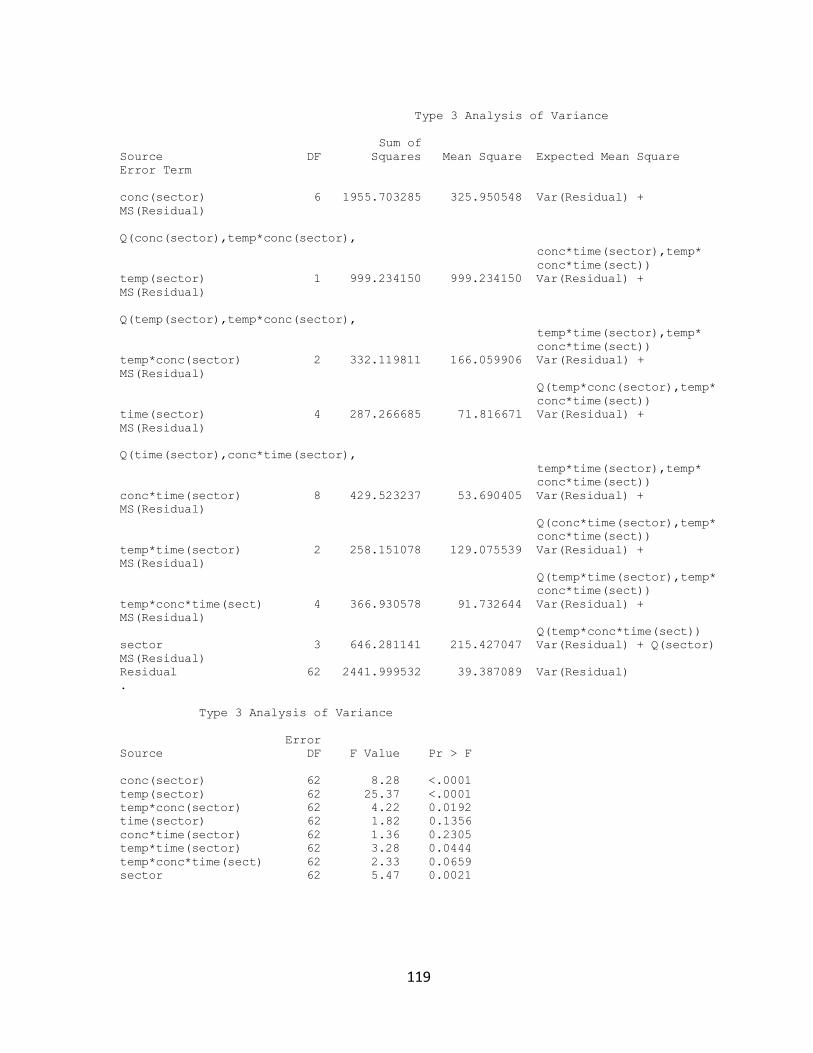
119
Type 3 Analysis of Variance
Sum of
Source DF Squares Mean Square Expected Mean Square
Error Term
conc(sector) 6 1955.703285 325.950548 Var(Residual) +
MS(Residual)
Q(conc(sector),temp*conc(sector),
conc*time(sector),temp*
conc*time(sect))
temp(sector) 1 999.234150 999.234150 Var(Residual) +
MS(Residual)
Q(temp(sector),temp*conc(sector),
temp*time(sector),temp*
conc*time(sect))
temp*conc(sector) 2 332.119811 166.059906 Var(Residual) +
MS(Residual)
Q(temp*conc(sector),temp*
conc*time(sect))
time(sector) 4 287.266685 71.816671 Var(Residual) +
MS(Residual)
Q(time(sector),conc*time(sector),
temp*time(sector),temp*
conc*time(sect))
conc*time(sector) 8 429.523237 53.690405 Var(Residual) +
MS(Residual)
Q(conc*time(sector),temp*
conc*time(sect))
temp*time(sector) 2 258.151078 129.075539 Var(Residual) +
MS(Residual)
Q(temp*time(sector),temp*
conc*time(sect))
temp*conc*time(sect) 4 366.930578 91.732644 Var(Residual) +
MS(Residual)
Q(temp*conc*time(sect))
sector 3 646.281141 215.427047 Var(Residual) + Q(sector)
MS(Residual)
Residual 62 2441.999532 39.387089 Var(Residual)
.
Type 3 Analysis of Variance
Error
Source DF F Value Pr > F
conc(sector) 62 8.28 <.0001
temp(sector) 62 25.37 <.0001
temp*conc(sector) 62 4.22 0.0192
time(sector) 62 1.82 0.1356
conc*time(sector) 62 1.36 0.2305
temp*time(sector) 62 3.28 0.0444
temp*conc*time(sect) 62 2.33 0.0659
sector 62 5.47 0.0021
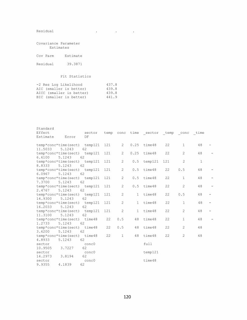
120
Residual . . .
Covariance Parameter
Estimates
Cov Parm Estimate
Residual 39.3871
Fit Statistics
-2 Res Log Likelihood 437.8
AIC (smaller is better) 439.8
AICC (smaller is better) 439.8
BIC (smaller is better) 441.9
Standard
Effect sector temp conc time _sector _temp _conc _time
Estimate Error DF
temp*conc*time(sect) temp121 121 2 0.25 time48 22 1 48 -
11.5033 5.1243 62
temp*conc*time(sect) temp121 121 2 0.25 time48 22 2 48 -
6.6100 5.1243 62
temp*conc*time(sect) temp121 121 2 0.5 temp121 121 2 1
8.8333 5.1243 62
temp*conc*time(sect) temp121 121 2 0.5 time48 22 0.5 48 -
6.0967 5.1243 62
temp*conc*time(sect) temp121 121 2 0.5 time48 22 1 48 -
7.3700 5.1243 62
temp*conc*time(sect) temp121 121 2 0.5 time48 22 2 48 -
2.4767 5.1243 62
temp*conc*time(sect) temp121 121 2 1 time48 22 0.5 48 -
14.9300 5.1243 62
temp*conc*time(sect) temp121 121 2 1 time48 22 1 48 -
16.2033 5.1243 62
temp*conc*time(sect) temp121 121 2 1 time48 22 2 48 -
11.3100 5.1243 62
temp*conc*time(sect) time48 22 0.5 48 time48 22 1 48 -
1.2733 5.1243 62
temp*conc*time(sect) time48 22 0.5 48 time48 22 2 48
3.6200 5.1243 62
temp*conc*time(sect) time48 22 1 48 time48 22 2 48
4.8933 5.1243 62
sector conc0 full
10.9505 3.7227 62
sector conc0 temp121
14.2973 3.8194 62
sector conc0 time48
9.9355 4.1839 62
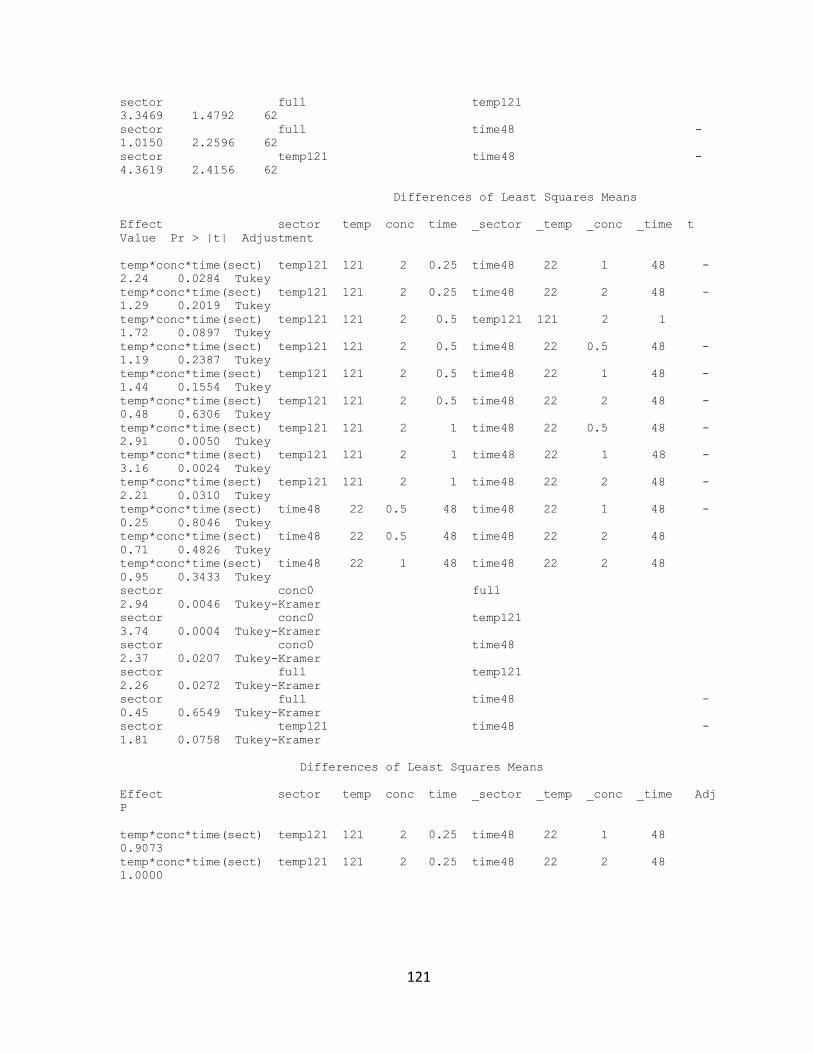
121
sector full temp121
3.3469 1.4792 62
sector full time48 -
1.0150 2.2596 62
sector temp121 time48 -
4.3619 2.4156 62
Differences of Least Squares Means
Effect sector temp conc time _sector _temp _conc _time t
Value Pr > |t| Adjustment
temp*conc*time(sect) temp121 121 2 0.25 time48 22 1 48 -
2.24 0.0284 Tukey
temp*conc*time(sect) temp121 121 2 0.25 time48 22 2 48 -
1.29 0.2019 Tukey
temp*conc*time(sect) temp121 121 2 0.5 temp121 121 2 1
1.72 0.0897 Tukey
temp*conc*time(sect) temp121 121 2 0.5 time48 22 0.5 48 -
1.19 0.2387 Tukey
temp*conc*time(sect) temp121 121 2 0.5 time48 22 1 48 -
1.44 0.1554 Tukey
temp*conc*time(sect) temp121 121 2 0.5 time48 22 2 48 -
0.48 0.6306 Tukey
temp*conc*time(sect) temp121 121 2 1 time48 22 0.5 48 -
2.91 0.0050 Tukey
temp*conc*time(sect) temp121 121 2 1 time48 22 1 48 -
3.16 0.0024 Tukey
temp*conc*time(sect) temp121 121 2 1 time48 22 2 48 -
2.21 0.0310 Tukey
temp*conc*time(sect) time48 22 0.5 48 time48 22 1 48 -
0.25 0.8046 Tukey
temp*conc*time(sect) time48 22 0.5 48 time48 22 2 48
0.71 0.4826 Tukey
temp*conc*time(sect) time48 22 1 48 time48 22 2 48
0.95 0.3433 Tukey
sector conc0 full
2.94 0.0046 Tukey-Kramer
sector conc0 temp121
3.74 0.0004 Tukey-Kramer
sector conc0 time48
2.37 0.0207 Tukey-Kramer
sector full temp121
2.26 0.0272 Tukey-Kramer
sector full time48 -
0.45 0.6549 Tukey-Kramer
sector temp121 time48 -
1.81 0.0758 Tukey-Kramer
Differences of Least Squares Means
Effect sector temp conc time _sector _temp _conc _time Adj
P
temp*conc*time(sect) temp121 121 2 0.25 time48 22 1 48
0.9073
temp*conc*time(sect) temp121 121 2 0.25 time48 22 2 48
1.0000
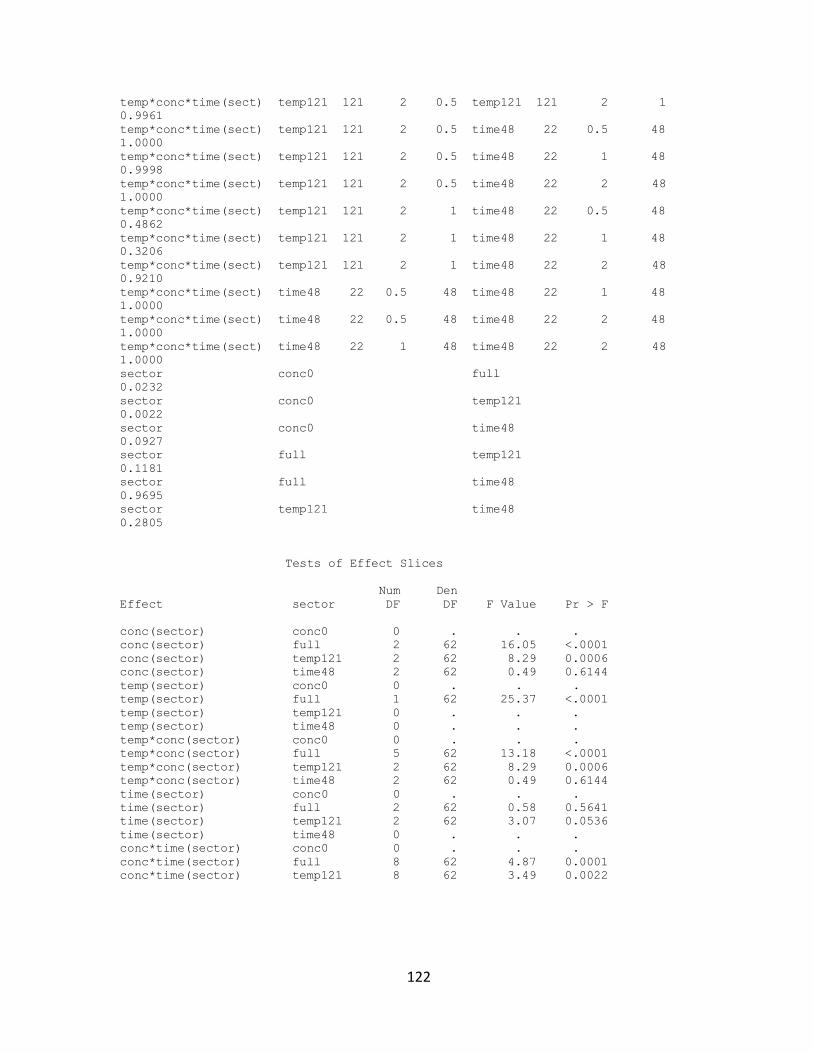
122
temp*conc*time(sect) temp121 121 2 0.5 temp121 121 2 1
0.9961
temp*conc*time(sect) temp121 121 2 0.5 time48 22 0.5 48
1.0000
temp*conc*time(sect) temp121 121 2 0.5 time48 22 1 48
0.9998
temp*conc*time(sect) temp121 121 2 0.5 time48 22 2 48
1.0000
temp*conc*time(sect) temp121 121 2 1 time48 22 0.5 48
0.4862
temp*conc*time(sect) temp121 121 2 1 time48 22 1 48
0.3206
temp*conc*time(sect) temp121 121 2 1 time48 22 2 48
0.9210
temp*conc*time(sect) time48 22 0.5 48 time48 22 1 48
1.0000
temp*conc*time(sect) time48 22 0.5 48 time48 22 2 48
1.0000
temp*conc*time(sect) time48 22 1 48 time48 22 2 48
1.0000
sector conc0 full
0.0232
sector conc0 temp121
0.0022
sector conc0 time48
0.0927
sector full temp121
0.1181
sector full time48
0.9695
sector temp121 time48
0.2805
Tests of Effect Slices
Num Den
Effect sector DF DF F Value Pr > F
conc(sector) conc0 0 . . .
conc(sector) full 2 62 16.05 <.0001
conc(sector) temp121 2 62 8.29 0.0006
conc(sector) time48 2 62 0.49 0.6144
temp(sector) conc0 0 . . .
temp(sector) full 1 62 25.37 <.0001
temp(sector) temp121 0 . . .
temp(sector) time48 0 . . .
temp*conc(sector) conc0 0 . . .
temp*conc(sector) full 5 62 13.18 <.0001
temp*conc(sector) temp121 2 62 8.29 0.0006
temp*conc(sector) time48 2 62 0.49 0.6144
time(sector) conc0 0 . . .
time(sector) full 2 62 0.58 0.5641
time(sector) temp121 2 62 3.07 0.0536
time(sector) time48 0 . . .
conc*time(sector) conc0 0 . . .
conc*time(sector) full 8 62 4.87 0.0001
conc*time(sector) temp121 8 62 3.49 0.0022
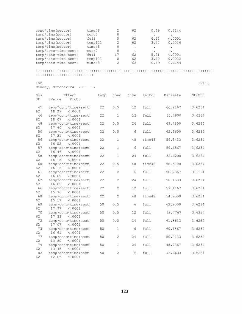
123
conc*time(sector) time48 2 62 0.49 0.6144
temp*time(sector) conc0 0 . . .
temp*time(sector) full 5 62 6.62 <.0001
temp*time(sector) temp121 2 62 3.07 0.0536
temp*time(sector) time48 0 . . .
temp*conc*time(sect) conc0 0 . . .
temp*conc*time(sect) full 17 62 5.21 <.0001
temp*conc*time(sect) temp121 8 62 3.49 0.0022
temp*conc*time(sect) time48 2 62 0.49 0.6144
+++++++++++++++++++++++++++++++++++++++++++++++++++++++++++++++++++++++++++++++++++
+++++++++++++++++++++++++++
lsm 19:30
Monday, October 24, 2011 67
Obs Effect temp conc time sector Estimate StdErr
DF tValue Probt
45 temp*conc*time(sect) 22 0.5 12 full 66.2167 3.6234
62 18.27 <.0001
46 temp*conc*time(sect) 22 1 12 full 65.4800 3.6234
62 18.07 <.0001
48 temp*conc*time(sect) 22 0.5 24 full 63.7800 3.6234
62 17.60 <.0001
50 temp*conc*time(sect) 22 0.5 6 full 62.3600 3.6234
62 17.21 <.0001
56 temp*conc*time(sect) 22 1 48 time48 59.8433 3.6234
62 16.52 <.0001
57 temp*conc*time(sect) 22 1 6 full 59.6567 3.6234
62 16.46 <.0001
58 temp*conc*time(sect) 22 1 24 full 58.6200 3.6234
62 16.18 <.0001
60 temp*conc*time(sect) 22 0.5 48 time48 58.5700 3.6234
62 16.16 <.0001
61 temp*conc*time(sect) 22 2 6 full 58.2867 3.6234
62 16.09 <.0001
62 temp*conc*time(sect) 22 2 24 full 58.1533 3.6234
62 16.05 <.0001
66 temp*conc*time(sect) 22 2 12 full 57.1167 3.6234
62 15.76 <.0001
68 temp*conc*time(sect) 22 2 48 time48 54.9500 3.6234
62 15.17 <.0001
69 temp*conc*time(sect) 50 0.5 6 full 62.9500 3.6234
62 17.37 <.0001
70 temp*conc*time(sect) 50 0.5 12 full 62.7767 3.6234
62 17.33 <.0001
72 temp*conc*time(sect) 50 0.5 24 full 61.8633 3.6234
62 17.07 <.0001
73 temp*conc*time(sect) 50 1 6 full 60.1867 3.6234
62 16.61 <.0001
77 temp*conc*time(sect) 50 2 24 full 50.0133 3.6234
62 13.80 <.0001
79 temp*conc*time(sect) 50 1 24 full 48.7367 3.6234
62 13.45 <.0001
82 temp*conc*time(sect) 50 2 6 full 43.6633 3.6234
62 12.05 <.0001
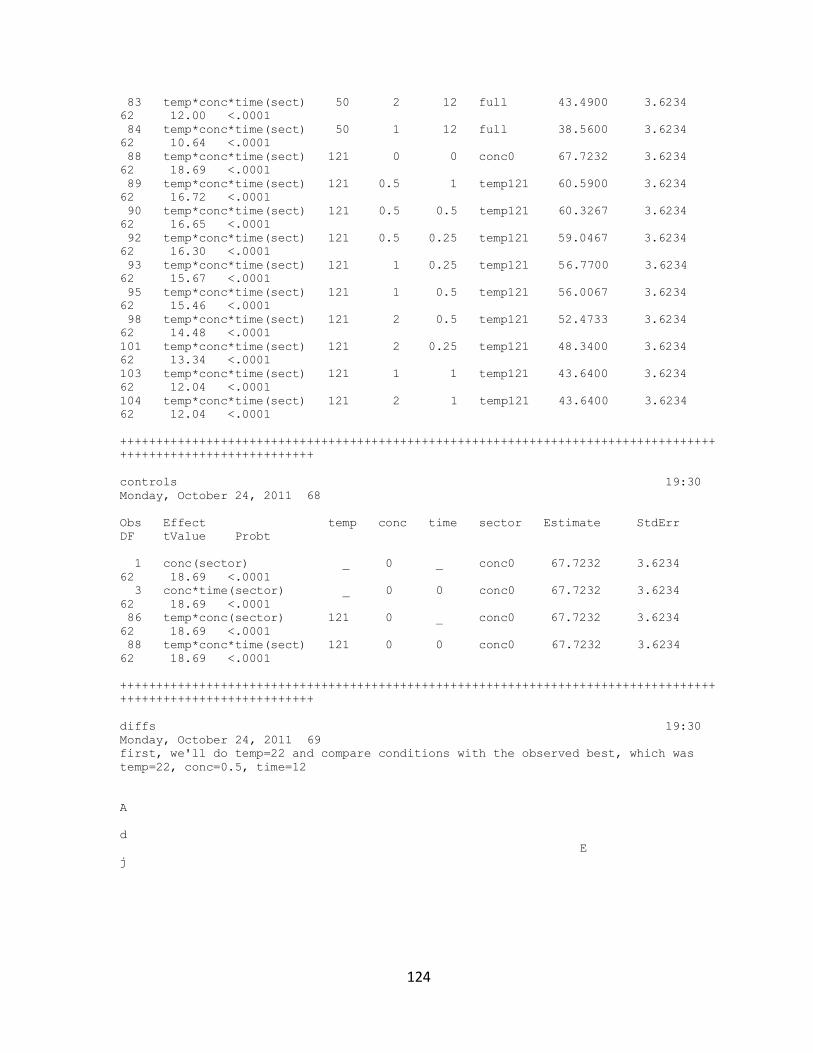
124
83 temp*conc*time(sect) 50 2 12 full 43.4900 3.6234
62 12.00 <.0001
84 temp*conc*time(sect) 50 1 12 full 38.5600 3.6234
62 10.64 <.0001
88 temp*conc*time(sect) 121 0 0 conc0 67.7232 3.6234
62 18.69 <.0001
89 temp*conc*time(sect) 121 0.5 1 temp121 60.5900 3.6234
62 16.72 <.0001
90 temp*conc*time(sect) 121 0.5 0.5 temp121 60.3267 3.6234
62 16.65 <.0001
92 temp*conc*time(sect) 121 0.5 0.25 temp121 59.0467 3.6234
62 16.30 <.0001
93 temp*conc*time(sect) 121 1 0.25 temp121 56.7700 3.6234
62 15.67 <.0001
95 temp*conc*time(sect) 121 1 0.5 temp121 56.0067 3.6234
62 15.46 <.0001
98 temp*conc*time(sect) 121 2 0.5 temp121 52.4733 3.6234
62 14.48 <.0001
101 temp*conc*time(sect) 121 2 0.25 temp121 48.3400 3.6234
62 13.34 <.0001
103 temp*conc*time(sect) 121 1 1 temp121 43.6400 3.6234
62 12.04 <.0001
104 temp*conc*time(sect) 121 2 1 temp121 43.6400 3.6234
62 12.04 <.0001
+++++++++++++++++++++++++++++++++++++++++++++++++++++++++++++++++++++++++++++++++++
+++++++++++++++++++++++++++
controls 19:30
Monday, October 24, 2011 68
Obs Effect temp conc time sector Estimate StdErr
DF tValue Probt
1 conc(sector) _ 0 _ conc0 67.7232 3.6234
62 18.69 <.0001
3 conc*time(sector) _ 0 0 conc0 67.7232 3.6234
62 18.69 <.0001
86 temp*conc(sector) 121 0 _ conc0 67.7232 3.6234
62 18.69 <.0001
88 temp*conc*time(sect) 121 0 0 conc0 67.7232 3.6234
62 18.69 <.0001
+++++++++++++++++++++++++++++++++++++++++++++++++++++++++++++++++++++++++++++++++++
+++++++++++++++++++++++++++
diffs 19:30
Monday, October 24, 2011 69
first, we'll do temp=22 and compare conditions with the observed best, which was
temp=22, conc=0.5, time=12
A
d
E
j
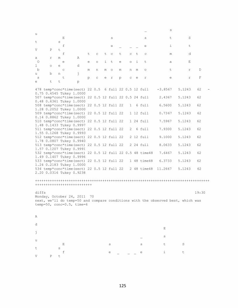
125
_ s
u
E s s t S
t s
f e _ _ _ e i t
V P t
f t c t c t c t c m d
a r m A
O e e o i t e o i t a E
l o e d
b c m n m o m n m o t r D
u b n j
s t p c e r p c e r e r F
e t t p
478 temp*conc*time(sect) 22 0.5 6 full 22 0.5 12 full -3.8567 5.1243 62 -
0.75 0.4545 Tukey 1.0000
507 temp*conc*time(sect) 22 0.5 12 full 22 0.5 24 full 2.4367 5.1243 62
0.48 0.6361 Tukey 1.0000
508 temp*conc*time(sect) 22 0.5 12 full 22 1 6 full 6.5600 5.1243 62
1.28 0.2052 Tukey 1.0000
509 temp*conc*time(sect) 22 0.5 12 full 22 1 12 full 0.7367 5.1243 62
0.14 0.8862 Tukey 1.0000
510 temp*conc*time(sect) 22 0.5 12 full 22 1 24 full 7.5967 5.1243 62
1.48 0.1433 Tukey 0.9997
511 temp*conc*time(sect) 22 0.5 12 full 22 2 6 full 7.9300 5.1243 62
1.55 0.1268 Tukey 0.9993
512 temp*conc*time(sect) 22 0.5 12 full 22 2 12 full 9.1000 5.1243 62
1.78 0.0807 Tukey 0.9940
513 temp*conc*time(sect) 22 0.5 12 full 22 2 24 full 8.0633 5.1243 62
1.57 0.1207 Tukey 0.9991
532 temp*conc*time(sect) 22 0.5 12 full 22 0.5 48 time48 7.6467 5.1243 62
1.49 0.1407 Tukey 0.9996
533 temp*conc*time(sect) 22 0.5 12 full 22 1 48 time48 6.3733 5.1243 62
1.24 0.2183 Tukey 1.0000
534 temp*conc*time(sect) 22 0.5 12 full 22 2 48 time48 11.2667 5.1243 62
2.20 0.0316 Tukey 0.9238
+++++++++++++++++++++++++++++++++++++++++++++++++++++++++++++++++++++++++++++++++++
+++++++++++++++++++++++++++
diffs 19:30
Monday, October 24, 2011 70
next, we'll do temp=50 and compare conditions with the observed best, which was
temp=50, conc=0.5, time=6
A
d
E
j
_ s
u
E s s t S
t s
f e _ _ _ e i t
V P t
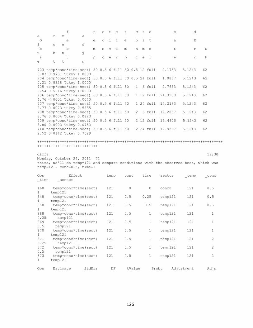
126
f t c t c t c t c m d
a r m A
O e e o i t e o i t a E
l o e d
b c m n m o m n m o t r D
u b n j
s t p c e r p c e r e r F
e t t p
703 temp*conc*time(sect) 50 0.5 6 full 50 0.5 12 full 0.1733 5.1243 62
0.03 0.9731 Tukey 1.0000
704 temp*conc*time(sect) 50 0.5 6 full 50 0.5 24 full 1.0867 5.1243 62
0.21 0.8328 Tukey 1.0000
705 temp*conc*time(sect) 50 0.5 6 full 50 1 6 full 2.7633 5.1243 62
0.54 0.5916 Tukey 1.0000
706 temp*conc*time(sect) 50 0.5 6 full 50 1 12 full 24.3900 5.1243 62
4.76 <.0001 Tukey 0.0040
707 temp*conc*time(sect) 50 0.5 6 full 50 1 24 full 14.2133 5.1243 62
2.77 0.0073 Tukey 0.5885
708 temp*conc*time(sect) 50 0.5 6 full 50 2 6 full 19.2867 5.1243 62
3.76 0.0004 Tukey 0.0823
709 temp*conc*time(sect) 50 0.5 6 full 50 2 12 full 19.4600 5.1243 62
3.80 0.0003 Tukey 0.0753
710 temp*conc*time(sect) 50 0.5 6 full 50 2 24 full 12.9367 5.1243 62
2.52 0.0142 Tukey 0.7629
+++++++++++++++++++++++++++++++++++++++++++++++++++++++++++++++++++++++++++++++++++
+++++++++++++++++++++++++++
diffs 19:30
Monday, October 24, 2011 71
third, we'll do temp=121 and compare conditions with the observed best, which was
temp=121, conc=0.5, time=1
Obs Effect temp conc time sector _temp _conc
_time _sector
468 temp*conc*time(sect) 121 0 0 conc0 121 0.5
1 temp121
848 temp*conc*time(sect) 121 0.5 0.25 temp121 121 0.5
1 temp121
858 temp*conc*time(sect) 121 0.5 0.5 temp121 121 0.5
1 temp121
868 temp*conc*time(sect) 121 0.5 1 temp121 121 1
0.25 temp121
869 temp*conc*time(sect) 121 0.5 1 temp121 121 1
0.5 temp121
870 temp*conc*time(sect) 121 0.5 1 temp121 121 1
1 temp121
871 temp*conc*time(sect) 121 0.5 1 temp121 121 2
0.25 temp121
872 temp*conc*time(sect) 121 0.5 1 temp121 121 2
0.5 temp121
873 temp*conc*time(sect) 121 0.5 1 temp121 121 2
1 temp121
Obs Estimate StdErr DF tValue Probt Adjustment Adjp
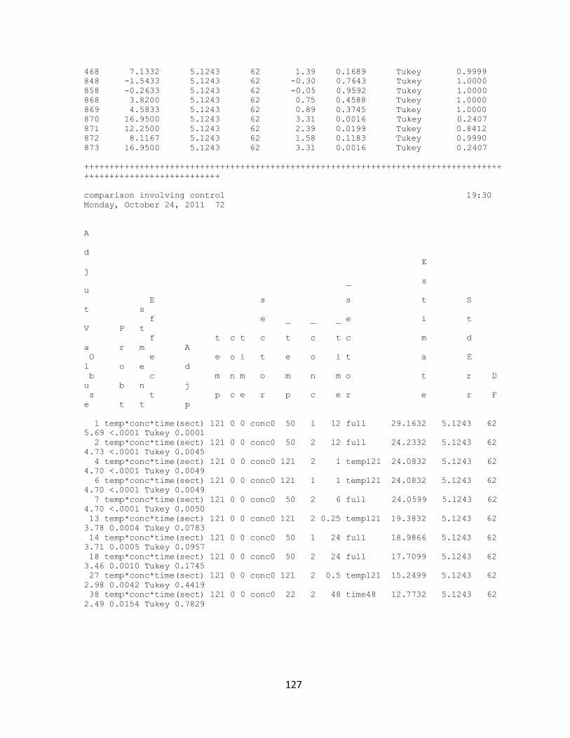
127
468 7.1332 5.1243 62 1.39 0.1689 Tukey 0.9999
848 -1.5433 5.1243 62 -0.30 0.7643 Tukey 1.0000
858 -0.2633 5.1243 62 -0.05 0.9592 Tukey 1.0000
868 3.8200 5.1243 62 0.75 0.4588 Tukey 1.0000
869 4.5833 5.1243 62 0.89 0.3745 Tukey 1.0000
870 16.9500 5.1243 62 3.31 0.0016 Tukey 0.2407
871 12.2500 5.1243 62 2.39 0.0199 Tukey 0.8412
872 8.1167 5.1243 62 1.58 0.1183 Tukey 0.9990
873 16.9500 5.1243 62 3.31 0.0016 Tukey 0.2407
+++++++++++++++++++++++++++++++++++++++++++++++++++++++++++++++++++++++++++++++++++
+++++++++++++++++++++++++++
comparison involving control 19:30
Monday, October 24, 2011 72
A
d
E
j
_ s
u
E s s t S
t s
f e _ _ _ e i t
V P t
f t c t c t c t c m d
a r m A
O e e o i t e o i t a E
l o e d
b c m n m o m n m o t r D
u b n j
s t p c e r p c e r e r F
e t t p
1 temp*conc*time(sect) 121 0 0 conc0 50 1 12 full 29.1632 5.1243 62
5.69 <.0001 Tukey 0.0001
2 temp*conc*time(sect) 121 0 0 conc0 50 2 12 full 24.2332 5.1243 62
4.73 <.0001 Tukey 0.0045
4 temp*conc*time(sect) 121 0 0 conc0 121 2 1 temp121 24.0832 5.1243 62
4.70 <.0001 Tukey 0.0049
6 temp*conc*time(sect) 121 0 0 conc0 121 1 1 temp121 24.0832 5.1243 62
4.70 <.0001 Tukey 0.0049
7 temp*conc*time(sect) 121 0 0 conc0 50 2 6 full 24.0599 5.1243 62
4.70 <.0001 Tukey 0.0050
13 temp*conc*time(sect) 121 0 0 conc0 121 2 0.25 temp121 19.3832 5.1243 62
3.78 0.0004 Tukey 0.0783
14 temp*conc*time(sect) 121 0 0 conc0 50 1 24 full 18.9866 5.1243 62
3.71 0.0005 Tukey 0.0957
18 temp*conc*time(sect) 121 0 0 conc0 50 2 24 full 17.7099 5.1243 62
3.46 0.0010 Tukey 0.1745
27 temp*conc*time(sect) 121 0 0 conc0 121 2 0.5 temp121 15.2499 5.1243 62
2.98 0.0042 Tukey 0.4419
38 temp*conc*time(sect) 121 0 0 conc0 22 2 48 time48 12.7732 5.1243 62
2.49 0.0154 Tukey 0.7829
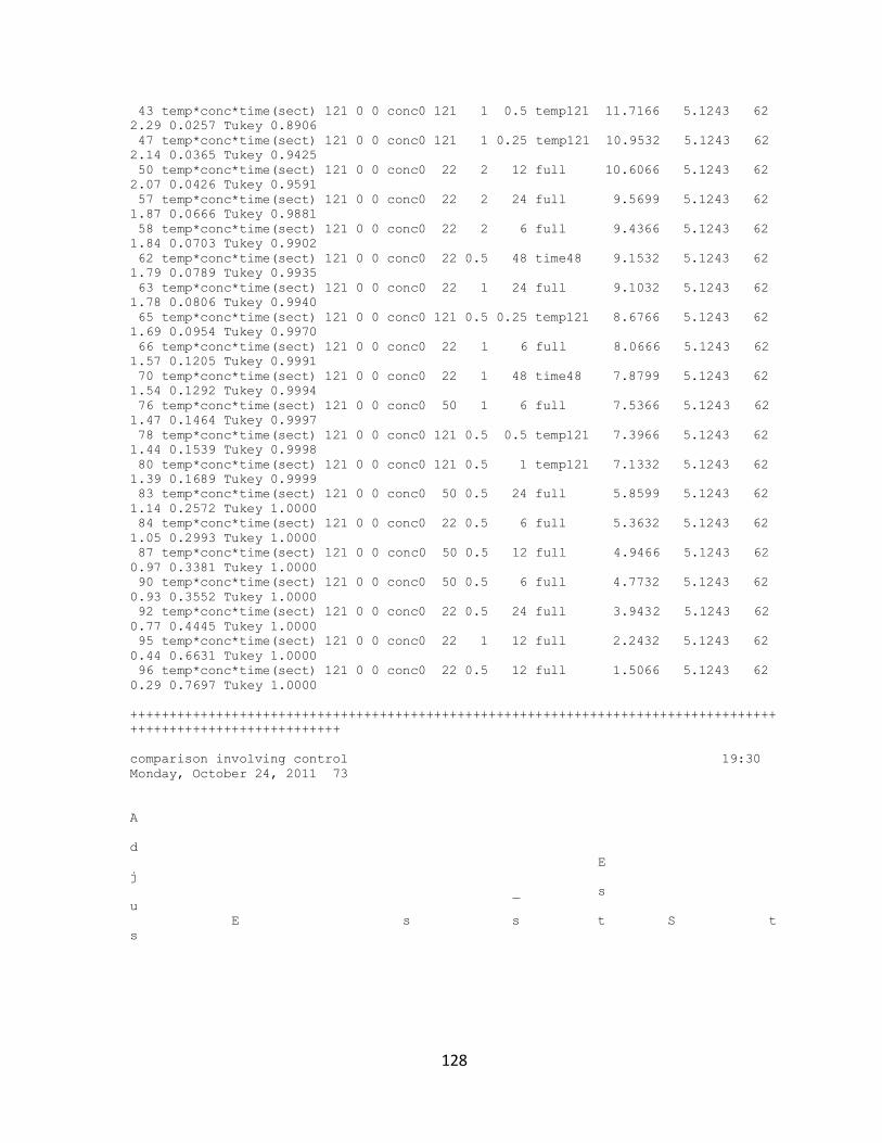
128
43 temp*conc*time(sect) 121 0 0 conc0 121 1 0.5 temp121 11.7166 5.1243 62
2.29 0.0257 Tukey 0.8906
47 temp*conc*time(sect) 121 0 0 conc0 121 1 0.25 temp121 10.9532 5.1243 62
2.14 0.0365 Tukey 0.9425
50 temp*conc*time(sect) 121 0 0 conc0 22 2 12 full 10.6066 5.1243 62
2.07 0.0426 Tukey 0.9591
57 temp*conc*time(sect) 121 0 0 conc0 22 2 24 full 9.5699 5.1243 62
1.87 0.0666 Tukey 0.9881
58 temp*conc*time(sect) 121 0 0 conc0 22 2 6 full 9.4366 5.1243 62
1.84 0.0703 Tukey 0.9902
62 temp*conc*time(sect) 121 0 0 conc0 22 0.5 48 time48 9.1532 5.1243 62
1.79 0.0789 Tukey 0.9935
63 temp*conc*time(sect) 121 0 0 conc0 22 1 24 full 9.1032 5.1243 62
1.78 0.0806 Tukey 0.9940
65 temp*conc*time(sect) 121 0 0 conc0 121 0.5 0.25 temp121 8.6766 5.1243 62
1.69 0.0954 Tukey 0.9970
66 temp*conc*time(sect) 121 0 0 conc0 22 1 6 full 8.0666 5.1243 62
1.57 0.1205 Tukey 0.9991
70 temp*conc*time(sect) 121 0 0 conc0 22 1 48 time48 7.8799 5.1243 62
1.54 0.1292 Tukey 0.9994
76 temp*conc*time(sect) 121 0 0 conc0 50 1 6 full 7.5366 5.1243 62
1.47 0.1464 Tukey 0.9997
78 temp*conc*time(sect) 121 0 0 conc0 121 0.5 0.5 temp121 7.3966 5.1243 62
1.44 0.1539 Tukey 0.9998
80 temp*conc*time(sect) 121 0 0 conc0 121 0.5 1 temp121 7.1332 5.1243 62
1.39 0.1689 Tukey 0.9999
83 temp*conc*time(sect) 121 0 0 conc0 50 0.5 24 full 5.8599 5.1243 62
1.14 0.2572 Tukey 1.0000
84 temp*conc*time(sect) 121 0 0 conc0 22 0.5 6 full 5.3632 5.1243 62
1.05 0.2993 Tukey 1.0000
87 temp*conc*time(sect) 121 0 0 conc0 50 0.5 12 full 4.9466 5.1243 62
0.97 0.3381 Tukey 1.0000
90 temp*conc*time(sect) 121 0 0 conc0 50 0.5 6 full 4.7732 5.1243 62
0.93 0.3552 Tukey 1.0000
92 temp*conc*time(sect) 121 0 0 conc0 22 0.5 24 full 3.9432 5.1243 62
0.77 0.4445 Tukey 1.0000
95 temp*conc*time(sect) 121 0 0 conc0 22 1 12 full 2.2432 5.1243 62
0.44 0.6631 Tukey 1.0000
96 temp*conc*time(sect) 121 0 0 conc0 22 0.5 12 full 1.5066 5.1243 62
0.29 0.7697 Tukey 1.0000
+++++++++++++++++++++++++++++++++++++++++++++++++++++++++++++++++++++++++++++++++++
+++++++++++++++++++++++++++
comparison involving control 19:30
Monday, October 24, 2011 73
A
d
E
j
_ s
u
E s s t S t
s
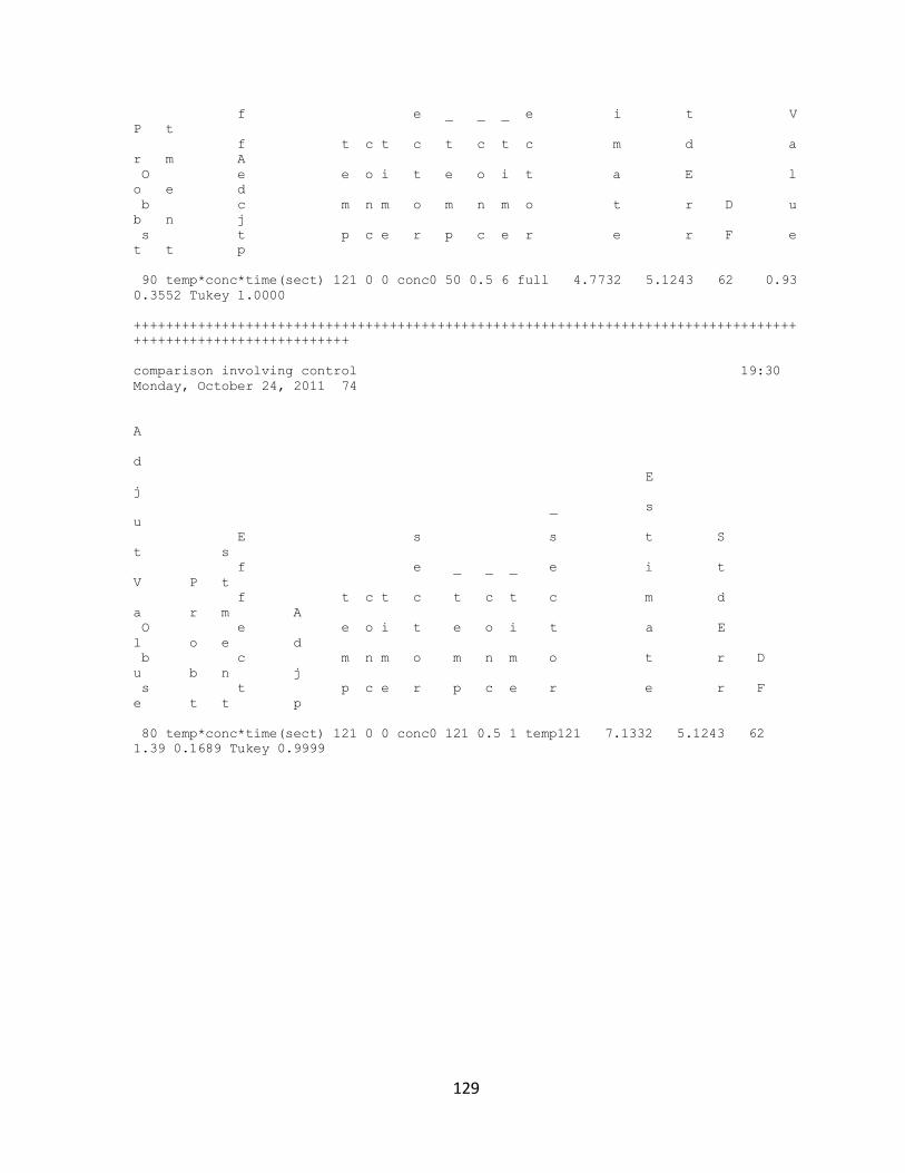
129
f e _ _ _ e i t V
P t
f t c t c t c t c m d a
r m A
O e e o i t e o i t a E l
o e d
b c m n m o m n m o t r D u
b n j
s t p c e r p c e r e r F e
t t p
90 temp*conc*time(sect) 121 0 0 conc0 50 0.5 6 full 4.7732 5.1243 62 0.93
0.3552 Tukey 1.0000
+++++++++++++++++++++++++++++++++++++++++++++++++++++++++++++++++++++++++++++++++++
+++++++++++++++++++++++++++
comparison involving control 19:30
Monday, October 24, 2011 74
A
d
E
j
_ s
u
E s s t S
t s
f e _ _ _ e i t
V P t
f t c t c t c t c m d
a r m A
O e e o i t e o i t a E
l o e d
b c m n m o m n m o t r D
u b n j
s t p c e r p c e r e r F
e t t p
80 temp*conc*time(sect) 121 0 0 conc0 121 0.5 1 temp121 7.1332 5.1243 62
1.39 0.1689 Tukey 0.9999
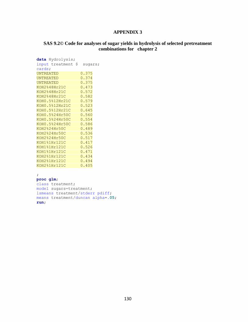
130
APPENDIX 3
SAS 9.2© Code for analyses of sugar yields in hydrolysis of selected pretreatment
combinations for chapter 2
data Hydrolysis;
input treatment $ sugars;
cards;
UNTREATED 0.375
UNTREATED 0.374
UNTREATED 0.375
KOH2%48Hr21C 0.473
KOH2%48Hr21C 0.572
KOH2%48Hr21C 0.582
KOH0.5%12Hr21C 0.579
KOH0.5%12Hr21C 0.523
KOH0.5%12Hr21C 0.645
KOH0.5%24Hr50C 0.560
KOH0.5%24Hr50C 0.554
KOH0.5%24Hr50C 0.586
KOH2%24Hr50C 0.489
KOH2%24Hr50C 0.536
KOH2%24Hr50C 0.517
KOH1%1Hr121C 0.417
KOH1%1Hr121C 0.526
KOH1%1Hr121C 0.471
KOH2%1Hr121C 0.434
KOH2%1Hr121C 0.494
KOH2%1Hr121C 0.405
;
proc glm;
class treatment;
model sugars=treatment;
lsmeans treatment/stderr pdiff;
means treatment/duncan alpha=.05;
run;
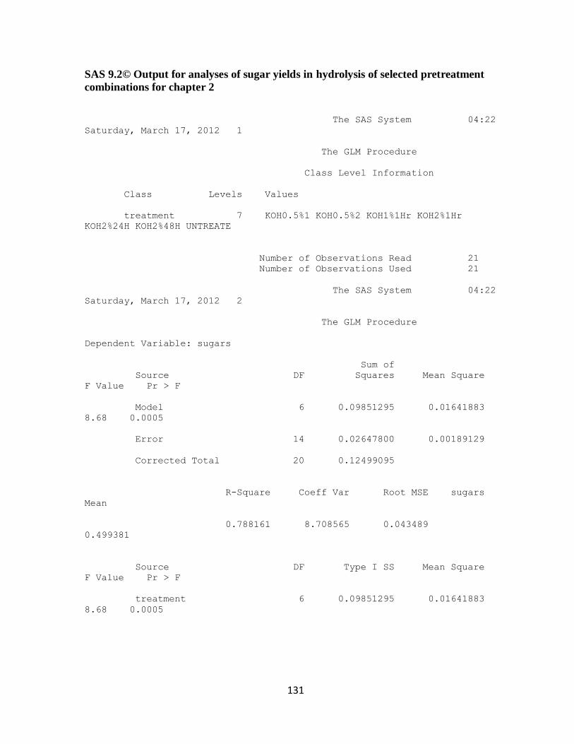
131
SAS 9.2© Output for analyses of sugar yields in hydrolysis of selected pretreatment
combinations for chapter 2
The SAS System 04:22
Saturday, March 17, 2012 1
The GLM Procedure
Class Level Information
Class Levels Values
treatment 7 KOH0.5%1 KOH0.5%2 KOH1%1Hr KOH2%1Hr
KOH2%24H KOH2%48H UNTREATE
Number of Observations Read 21
Number of Observations Used 21
The SAS System 04:22
Saturday, March 17, 2012 2
The GLM Procedure
Dependent Variable: sugars
Sum of
Source DF Squares Mean Square
F Value Pr > F
Model 6 0.09851295 0.01641883
8.68 0.0005
Error 14 0.02647800 0.00189129
Corrected Total 20 0.12499095
R-Square Coeff Var Root MSE sugars
Mean
0.788161 8.708565 0.043489
0.499381
Source DF Type I SS Mean Square
F Value Pr > F
treatment 6 0.09851295 0.01641883
8.68 0.0005
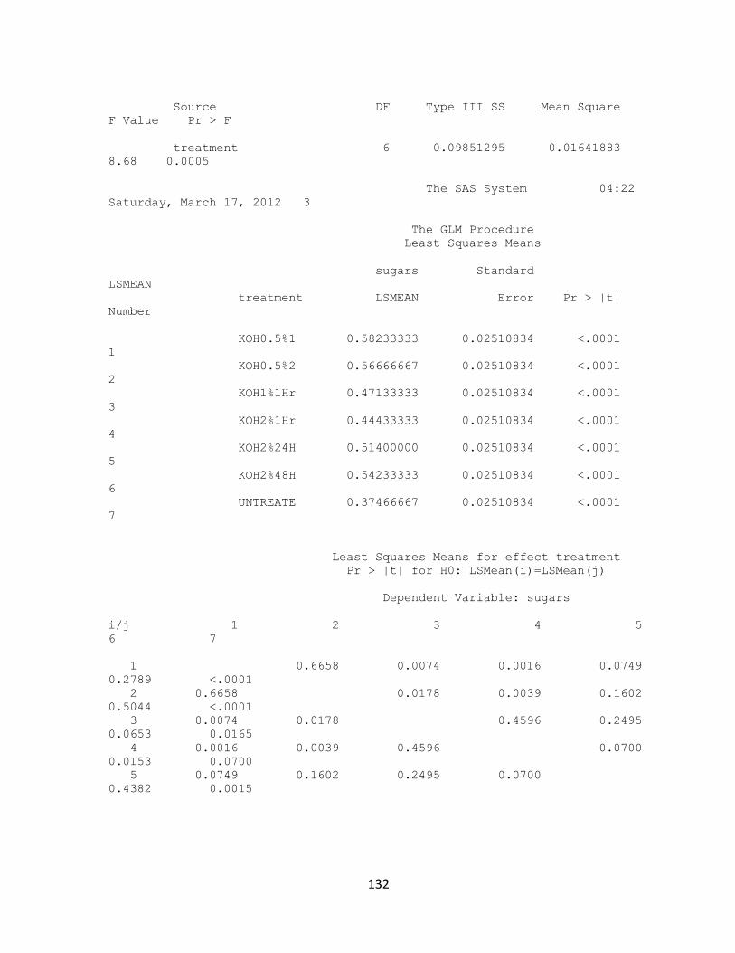
132
Source DF Type III SS Mean Square
F Value Pr > F
treatment 6 0.09851295 0.01641883
8.68 0.0005
The SAS System 04:22
Saturday, March 17, 2012 3
The GLM Procedure
Least Squares Means
sugars Standard
LSMEAN
treatment LSMEAN Error Pr > |t|
Number
KOH0.5%1 0.58233333 0.02510834 <.0001
1
KOH0.5%2 0.56666667 0.02510834 <.0001
2
KOH1%1Hr 0.47133333 0.02510834 <.0001
3
KOH2%1Hr 0.44433333 0.02510834 <.0001
4
KOH2%24H 0.51400000 0.02510834 <.0001
5
KOH2%48H 0.54233333 0.02510834 <.0001
6
UNTREATE 0.37466667 0.02510834 <.0001
7
Least Squares Means for effect treatment
Pr > |t| for H0: LSMean(i)=LSMean(j)
Dependent Variable: sugars
i/j 1 2 3 4 5
6 7
1 0.6658 0.0074 0.0016 0.0749
0.2789 <.0001
2 0.6658 0.0178 0.0039 0.1602
0.5044 <.0001
3 0.0074 0.0178 0.4596 0.2495
0.0653 0.0165
4 0.0016 0.0039 0.4596 0.0700
0.0153 0.0700
5 0.0749 0.1602 0.2495 0.0700
0.4382 0.0015
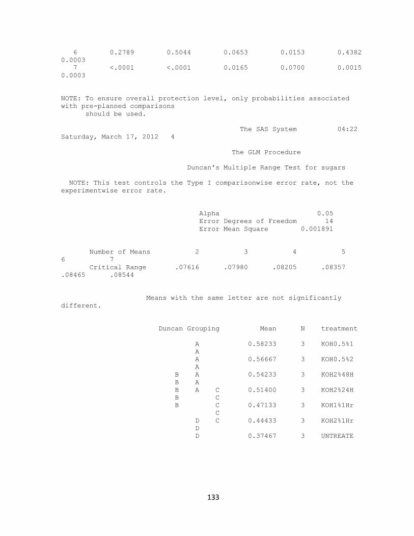
133
6 0.2789 0.5044 0.0653 0.0153 0.4382
0.0003
7 <.0001 <.0001 0.0165 0.0700 0.0015
0.0003
NOTE: To ensure overall protection level, only probabilities associated
with pre-planned comparisons
should be used.
The SAS System 04:22
Saturday, March 17, 2012 4
The GLM Procedure
Duncan's Multiple Range Test for sugars
NOTE: This test controls the Type I comparisonwise error rate, not the
experimentwise error rate.
Alpha 0.05
Error Degrees of Freedom 14
Error Mean Square 0.001891
Number of Means 2 3 4 5
6 7
Critical Range .07616 .07980 .08205 .08357
.08465 .08544
Means with the same letter are not significantly
different.
Duncan Grouping Mean N treatment
A 0.58233 3 KOH0.5%1
A
A 0.56667 3 KOH0.5%2
A
B A 0.54233 3 KOH2%48H
B A
B A C 0.51400 3 KOH2%24H
B C
B C 0.47133 3 KOH1%1Hr
C
D C 0.44433 3 KOH2%1Hr
D
D 0.37467 3 UNTREATE

134
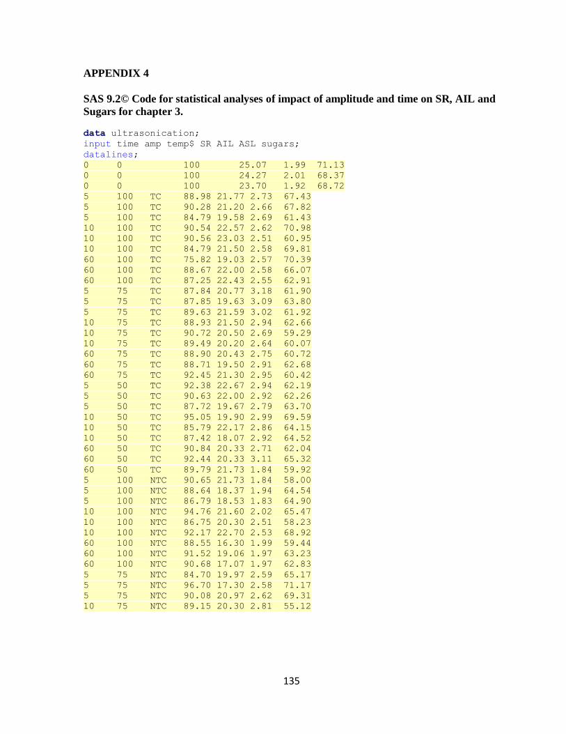
135
APPENDIX 4
SAS 9.2© Code for statistical analyses of impact of amplitude and time on SR, AIL and
Sugars for chapter 3.
data ultrasonication;
input time amp temp$ SR AIL ASL sugars;
datalines;
0 0 100 25.07 1.99 71.13
0 0 100 24.27 2.01 68.37
0 0 100 23.70 1.92 68.72
5 100 TC 88.98 21.77 2.73 67.43
5 100 TC 90.28 21.20 2.66 67.82
5 100 TC 84.79 19.58 2.69 61.43
10 100 TC 90.54 22.57 2.62 70.98
10 100 TC 90.56 23.03 2.51 60.95
10 100 TC 84.79 21.50 2.58 69.81
60 100 TC 75.82 19.03 2.57 70.39
60 100 TC 88.67 22.00 2.58 66.07
60 100 TC 87.25 22.43 2.55 62.91
5 75 TC 87.84 20.77 3.18 61.90
5 75 TC 87.85 19.63 3.09 63.80
5 75 TC 89.63 21.59 3.02 61.92
10 75 TC 88.93 21.50 2.94 62.66
10 75 TC 90.72 20.50 2.69 59.29
10 75 TC 89.49 20.20 2.64 60.07
60 75 TC 88.90 20.43 2.75 60.72
60 75 TC 88.71 19.50 2.91 62.68
60 75 TC 92.45 21.30 2.95 60.42
5 50 TC 92.38 22.67 2.94 62.19
5 50 TC 90.63 22.00 2.92 62.26
5 50 TC 87.72 19.67 2.79 63.70
10 50 TC 95.05 19.90 2.99 69.59
10 50 TC 85.79 22.17 2.86 64.15
10 50 TC 87.42 18.07 2.92 64.52
60 50 TC 90.84 20.33 2.71 62.04
60 50 TC 92.44 20.33 3.11 65.32
60 50 TC 89.79 21.73 1.84 59.92
5 100 NTC 90.65 21.73 1.84 58.00
5 100 NTC 88.64 18.37 1.94 64.54
5 100 NTC 86.79 18.53 1.83 64.90
10 100 NTC 94.76 21.60 2.02 65.47
10 100 NTC 86.75 20.30 2.51 58.23
10 100 NTC 92.17 22.70 2.53 68.92
60 100 NTC 88.55 16.30 1.99 59.44
60 100 NTC 91.52 19.06 1.97 63.23
60 100 NTC 90.68 17.07 1.97 62.83
5 75 NTC 84.70 19.97 2.59 65.17
5 75 NTC 96.70 17.30 2.58 71.17
5 75 NTC 90.08 20.97 2.62 69.31
10 75 NTC 89.15 20.30 2.81 55.12
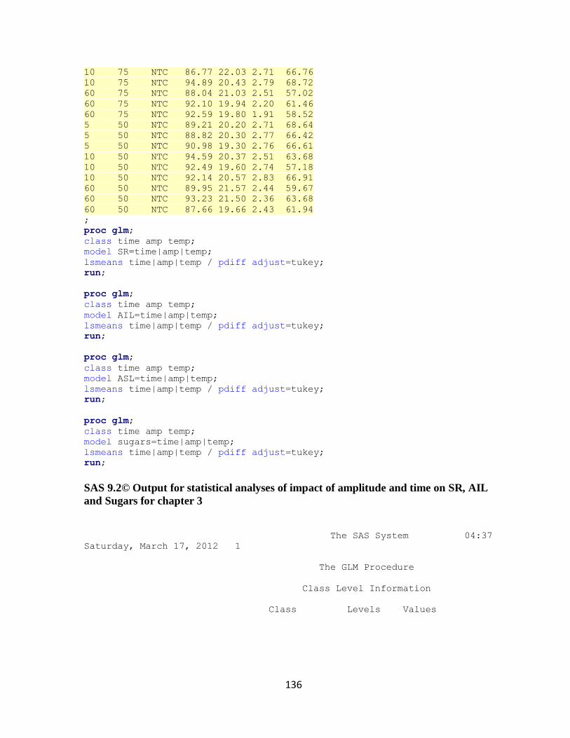
136
10 75 NTC 86.77 22.03 2.71 66.76
10 75 NTC 94.89 20.43 2.79 68.72
60 75 NTC 88.04 21.03 2.51 57.02
60 75 NTC 92.10 19.94 2.20 61.46
60 75 NTC 92.59 19.80 1.91 58.52
5 50 NTC 89.21 20.20 2.71 68.64
5 50 NTC 88.82 20.30 2.77 66.42
5 50 NTC 90.98 19.30 2.76 66.61
10 50 NTC 94.59 20.37 2.51 63.68
10 50 NTC 92.49 19.60 2.74 57.18
10 50 NTC 92.14 20.57 2.83 66.91
60 50 NTC 89.95 21.57 2.44 59.67
60 50 NTC 93.23 21.50 2.36 63.68
60 50 NTC 87.66 19.66 2.43 61.94
;
proc glm;
class time amp temp;
model SR=time|amp|temp;
lsmeans time|amp|temp / pdiff adjust=tukey;
run;
proc glm;
class time amp temp;
model AIL=time|amp|temp;
lsmeans time|amp|temp / pdiff adjust=tukey;
run;
proc glm;
class time amp temp;
model ASL=time|amp|temp;
lsmeans time|amp|temp / pdiff adjust=tukey;
run;
proc glm;
class time amp temp;
model sugars=time|amp|temp;
lsmeans time|amp|temp / pdiff adjust=tukey;
run;
SAS 9.2© Output for statistical analyses of impact of amplitude and time on SR, AIL
and Sugars for chapter 3
The SAS System 04:37
Saturday, March 17, 2012 1
The GLM Procedure
Class Level Information
Class Levels Values
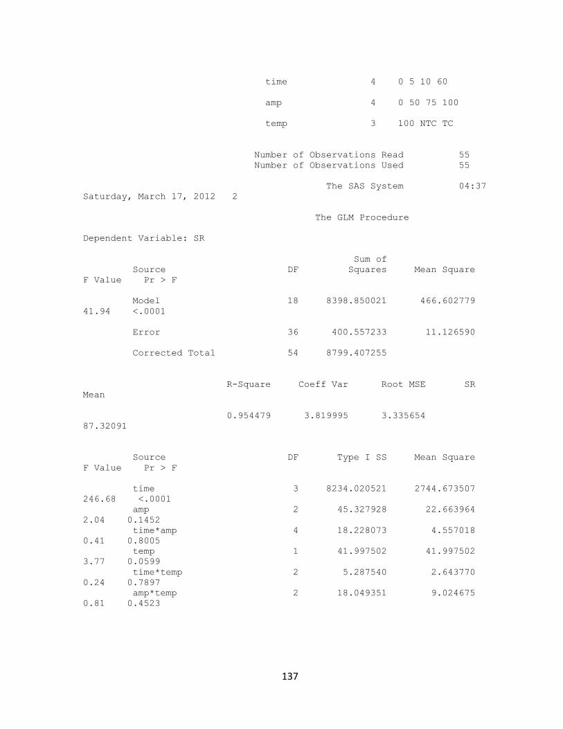
137
time 4 0 5 10 60
amp 4 0 50 75 100
temp 3 100 NTC TC
Number of Observations Read 55
Number of Observations Used 55
The SAS System 04:37
Saturday, March 17, 2012 2
The GLM Procedure
Dependent Variable: SR
Sum of
Source DF Squares Mean Square
F Value Pr > F
Model 18 8398.850021 466.602779
41.94 <.0001
Error 36 400.557233 11.126590
Corrected Total 54 8799.407255
R-Square Coeff Var Root MSE SR
Mean
0.954479 3.819995 3.335654
87.32091
Source DF Type I SS Mean Square
F Value Pr > F
time 3 8234.020521 2744.673507
246.68 <.0001
amp 2 45.327928 22.663964
2.04 0.1452
time*amp 4 18.228073 4.557018
0.41 0.8005
temp 1 41.997502 41.997502
3.77 0.0599
time*temp 2 5.287540 2.643770
0.24 0.7897
amp*temp 2 18.049351 9.024675
0.81 0.4523
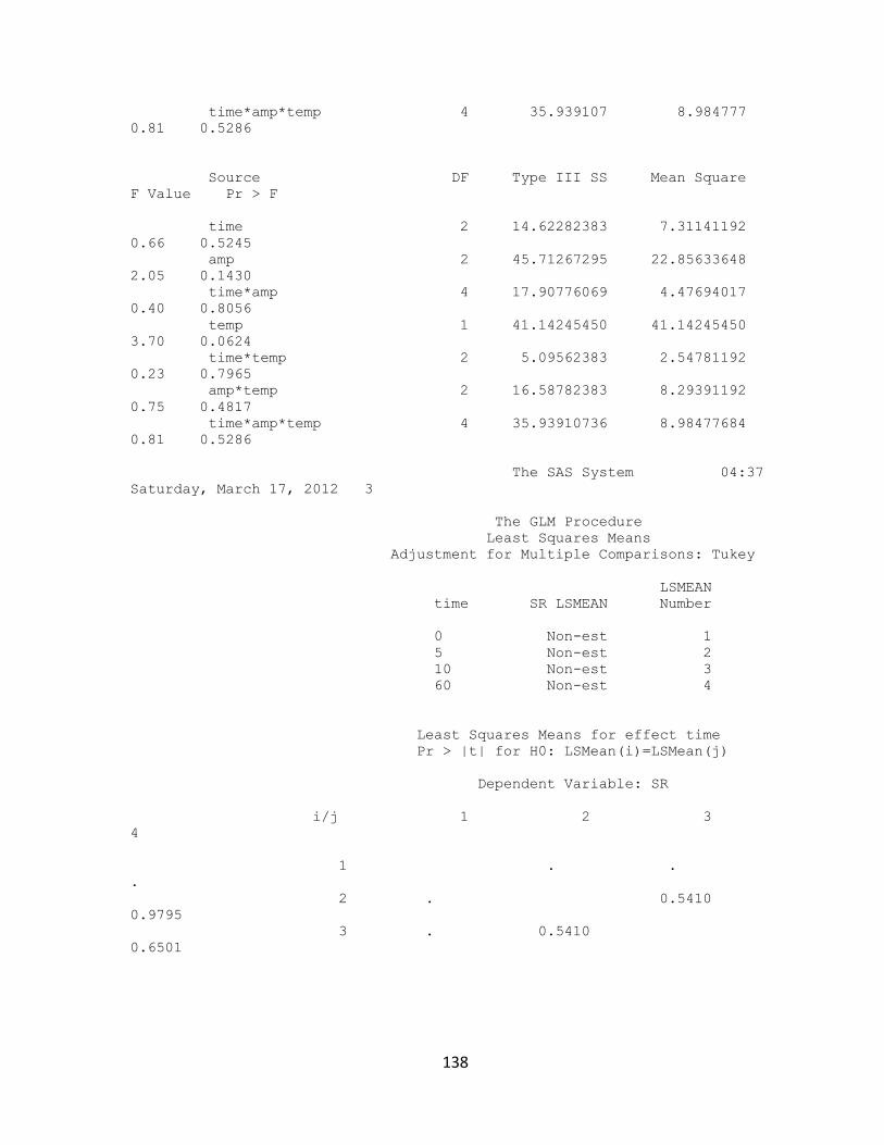
138
time*amp*temp 4 35.939107 8.984777
0.81 0.5286
Source DF Type III SS Mean Square
F Value Pr > F
time 2 14.62282383 7.31141192
0.66 0.5245
amp 2 45.71267295 22.85633648
2.05 0.1430
time*amp 4 17.90776069 4.47694017
0.40 0.8056
temp 1 41.14245450 41.14245450
3.70 0.0624
time*temp 2 5.09562383 2.54781192
0.23 0.7965
amp*temp 2 16.58782383 8.29391192
0.75 0.4817
time*amp*temp 4 35.93910736 8.98477684
0.81 0.5286
The SAS System 04:37
Saturday, March 17, 2012 3
The GLM Procedure
Least Squares Means
Adjustment for Multiple Comparisons: Tukey
LSMEAN
time SR LSMEAN Number
0 Non-est 1
5 Non-est 2
10 Non-est 3
60 Non-est 4
Least Squares Means for effect time
Pr > |t| for H0: LSMean(i)=LSMean(j)
Dependent Variable: SR
i/j 1 2 3
4
1 . .
.
2 . 0.5410
0.9795
3 . 0.5410
0.6501
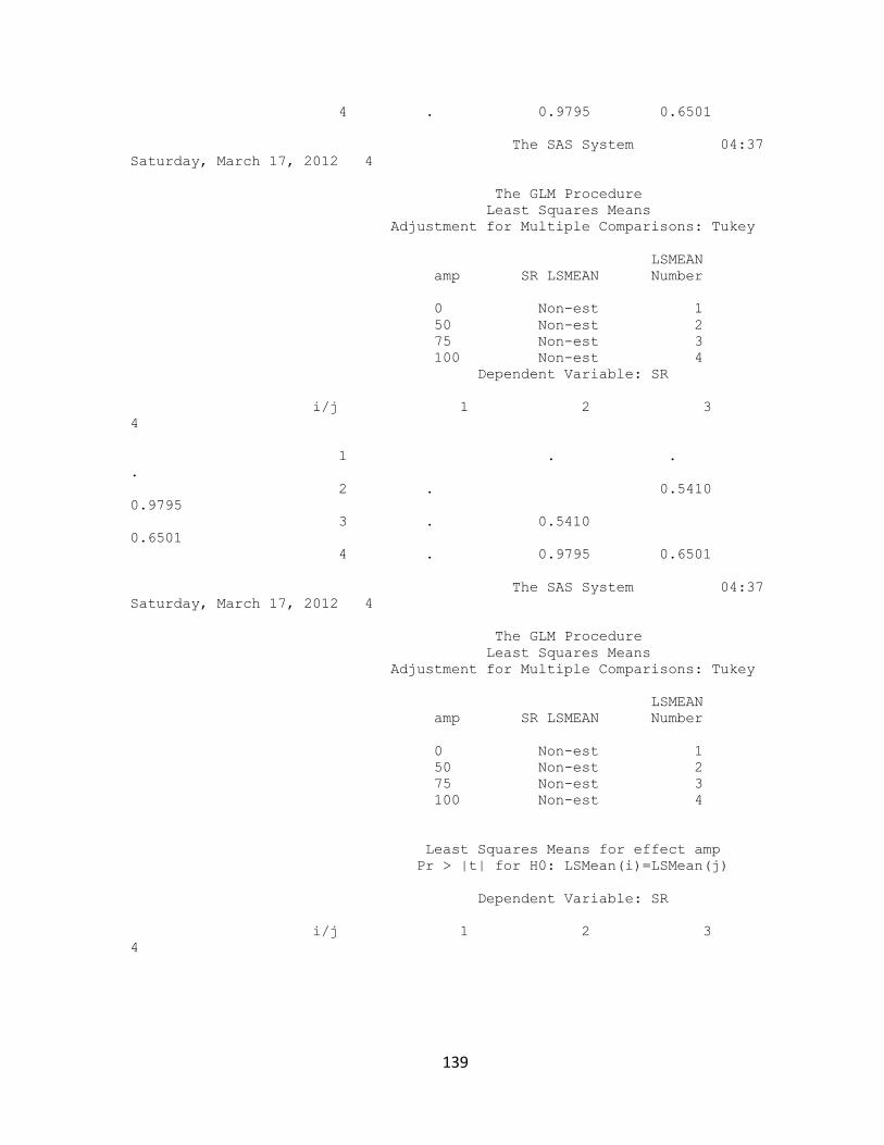
139
4 . 0.9795 0.6501
The SAS System 04:37
Saturday, March 17, 2012 4
The GLM Procedure
Least Squares Means
Adjustment for Multiple Comparisons: Tukey
LSMEAN
amp SR LSMEAN Number
0 Non-est 1
50 Non-est 2
75 Non-est 3
100 Non-est 4
Dependent Variable: SR
i/j 1 2 3
4
1 . .
.
2 . 0.5410
0.9795
3 . 0.5410
0.6501
4 . 0.9795 0.6501
The SAS System 04:37
Saturday, March 17, 2012 4
The GLM Procedure
Least Squares Means
Adjustment for Multiple Comparisons: Tukey
LSMEAN
amp SR LSMEAN Number
0 Non-est 1
50 Non-est 2
75 Non-est 3
100 Non-est 4
Least Squares Means for effect amp
Pr > |t| for H0: LSMean(i)=LSMean(j)
Dependent Variable: SR
i/j 1 2 3
4
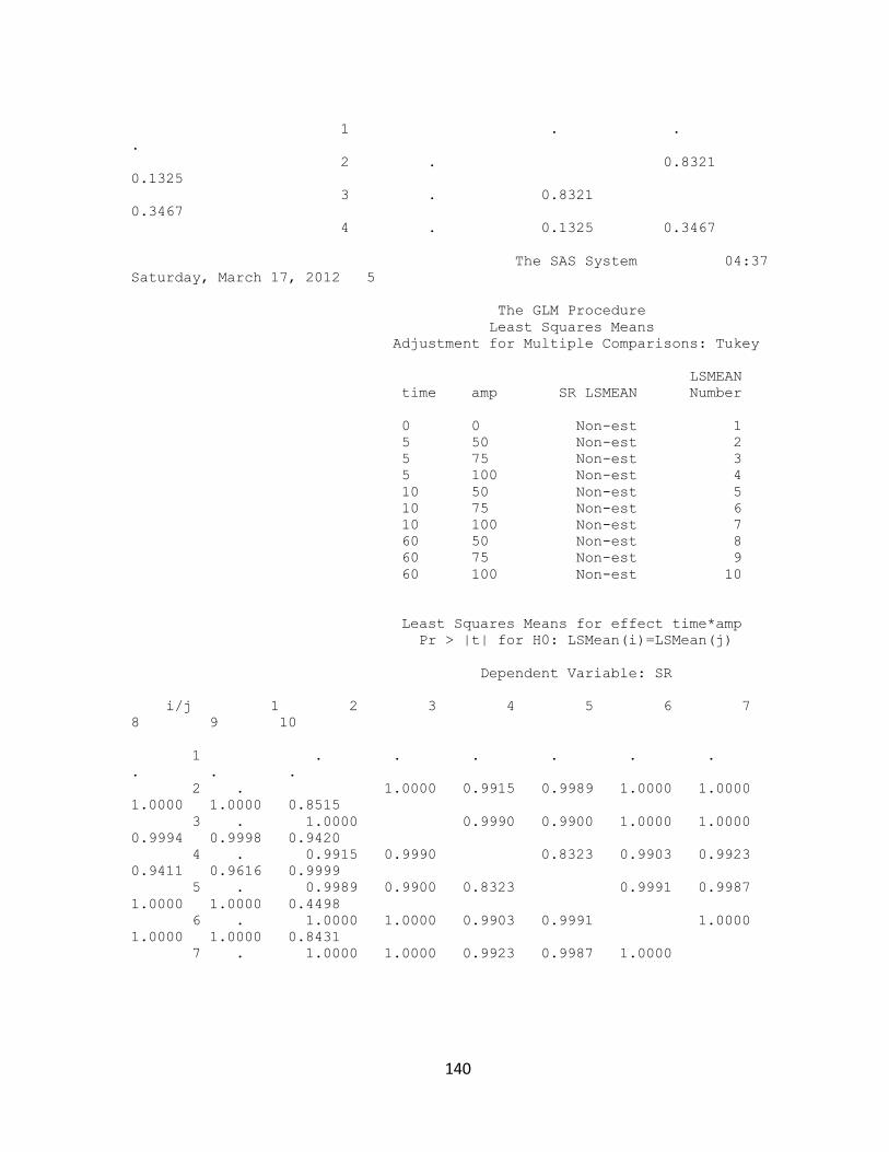
140
1 . .
.
2 . 0.8321
0.1325
3 . 0.8321
0.3467
4 . 0.1325 0.3467
The SAS System 04:37
Saturday, March 17, 2012 5
The GLM Procedure
Least Squares Means
Adjustment for Multiple Comparisons: Tukey
LSMEAN
time amp SR LSMEAN Number
0 0 Non-est 1
5 50 Non-est 2
5 75 Non-est 3
5 100 Non-est 4
10 50 Non-est 5
10 75 Non-est 6
10 100 Non-est 7
60 50 Non-est 8
60 75 Non-est 9
60 100 Non-est 10
Least Squares Means for effect time*amp
Pr > |t| for H0: LSMean(i)=LSMean(j)
Dependent Variable: SR
i/j 1 2 3 4 5 6 7
8 9 10
1 . . . . . .
. . .
2 . 1.0000 0.9915 0.9989 1.0000 1.0000
1.0000 1.0000 0.8515
3 . 1.0000 0.9990 0.9900 1.0000 1.0000
0.9994 0.9998 0.9420
4 . 0.9915 0.9990 0.8323 0.9903 0.9923
0.9411 0.9616 0.9999
5 . 0.9989 0.9900 0.8323 0.9991 0.9987
1.0000 1.0000 0.4498
6 . 1.0000 1.0000 0.9903 0.9991 1.0000
1.0000 1.0000 0.8431
7 . 1.0000 1.0000 0.9923 0.9987 1.0000
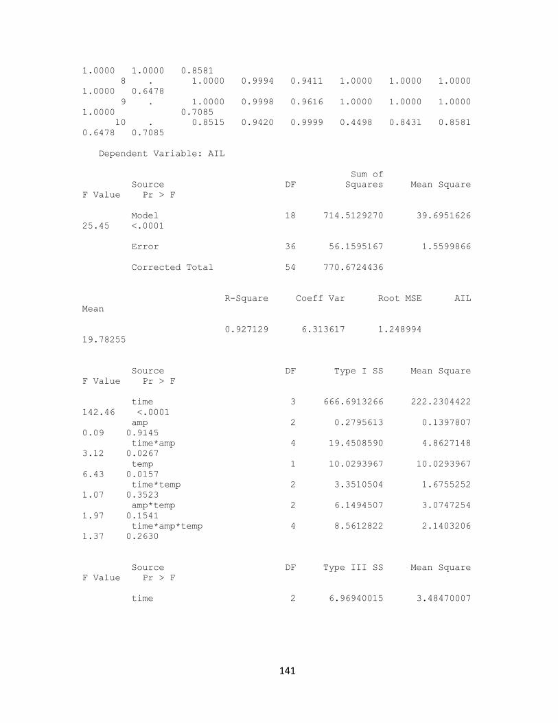
141
1.0000 1.0000 0.8581
8 . 1.0000 0.9994 0.9411 1.0000 1.0000 1.0000
1.0000 0.6478
9 . 1.0000 0.9998 0.9616 1.0000 1.0000 1.0000
1.0000 0.7085
10 . 0.8515 0.9420 0.9999 0.4498 0.8431 0.8581
0.6478 0.7085
Dependent Variable: AIL
Sum of
Source DF Squares Mean Square
F Value Pr > F
Model 18 714.5129270 39.6951626
25.45 <.0001
Error 36 56.1595167 1.5599866
Corrected Total 54 770.6724436
R-Square Coeff Var Root MSE AIL
Mean
0.927129 6.313617 1.248994
19.78255
Source DF Type I SS Mean Square
F Value Pr > F
time 3 666.6913266 222.2304422
142.46 <.0001
amp 2 0.2795613 0.1397807
0.09 0.9145
time*amp 4 19.4508590 4.8627148
3.12 0.0267
temp 1 10.0293967 10.0293967
6.43 0.0157
time*temp 2 3.3510504 1.6755252
1.07 0.3523
amp*temp 2 6.1494507 3.0747254
1.97 0.1541
time*amp*temp 4 8.5612822 2.1403206
1.37 0.2630
Source DF Type III SS Mean Square
F Value Pr > F
time 2 6.96940015 3.48470007
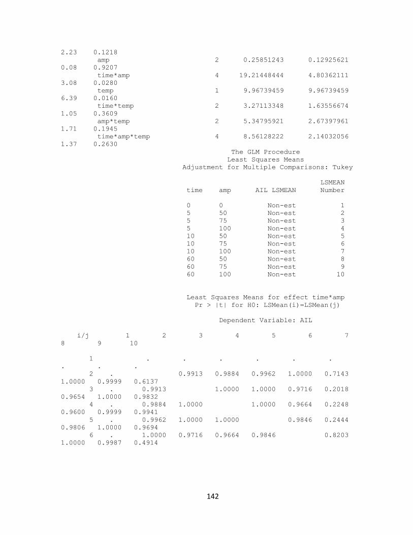
142
2.23 0.1218
amp 2 0.25851243 0.12925621
0.08 0.9207
time*amp 4 19.21448444 4.80362111
3.08 0.0280
temp 1 9.96739459 9.96739459
6.39 0.0160
time*temp 2 3.27113348 1.63556674
1.05 0.3609
amp*temp 2 5.34795921 2.67397961
1.71 0.1945
time*amp*temp 4 8.56128222 2.14032056
1.37 0.2630
The GLM Procedure
Least Squares Means
Adjustment for Multiple Comparisons: Tukey
LSMEAN
time amp AIL LSMEAN Number
0 0 Non-est 1
5 50 Non-est 2
5 75 Non-est 3
5 100 Non-est 4
10 50 Non-est 5
10 75 Non-est 6
10 100 Non-est 7
60 50 Non-est 8
60 75 Non-est 9
60 100 Non-est 10
Least Squares Means for effect time*amp
Pr > |t| for H0: LSMean(i)=LSMean(j)
Dependent Variable: AIL
i/j 1 2 3 4 5 6 7
8 9 10
1 . . . . . .
. . .
2 . 0.9913 0.9884 0.9962 1.0000 0.7143
1.0000 0.9999 0.6137
3 . 0.9913 1.0000 1.0000 0.9716 0.2018
0.9654 1.0000 0.9832
4 . 0.9884 1.0000 1.0000 0.9664 0.2248
0.9600 0.9999 0.9941
5 . 0.9962 1.0000 1.0000 0.9846 0.2444
0.9806 1.0000 0.9694
6 . 1.0000 0.9716 0.9664 0.9846 0.8203
1.0000 0.9987 0.4914
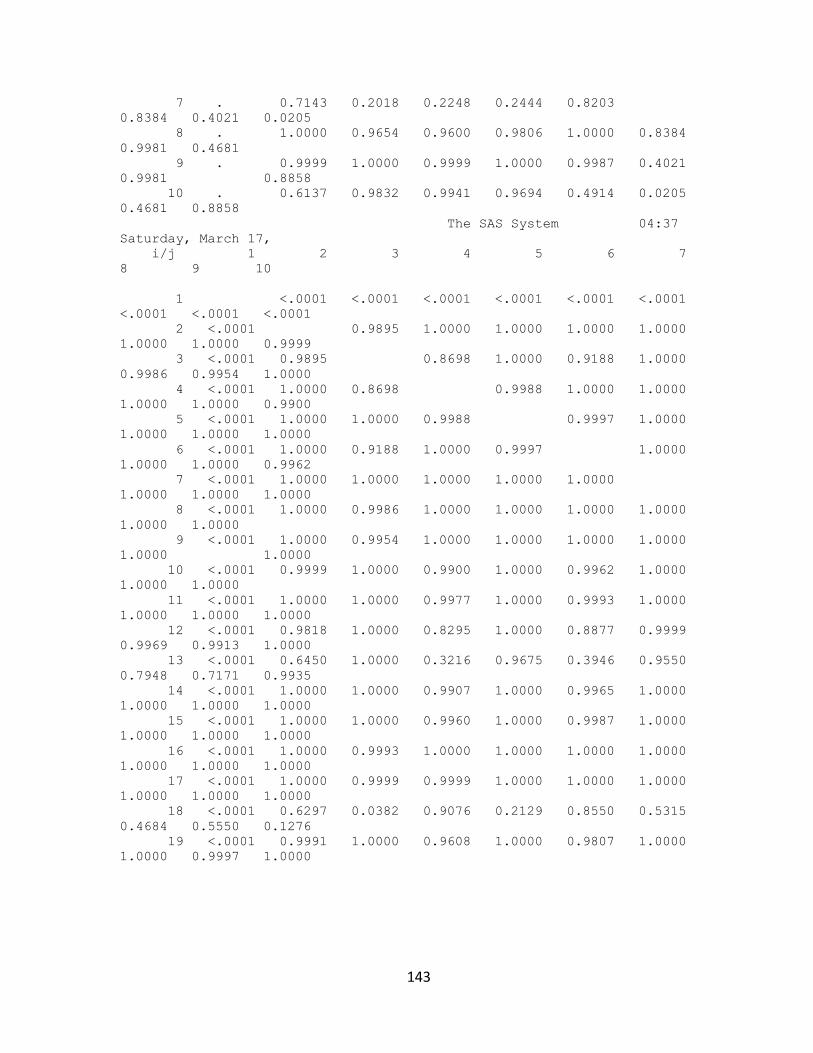
143
7 . 0.7143 0.2018 0.2248 0.2444 0.8203
0.8384 0.4021 0.0205
8 . 1.0000 0.9654 0.9600 0.9806 1.0000 0.8384
0.9981 0.4681
9 . 0.9999 1.0000 0.9999 1.0000 0.9987 0.4021
0.9981 0.8858
10 . 0.6137 0.9832 0.9941 0.9694 0.4914 0.0205
0.4681 0.8858
The SAS System 04:37
Saturday, March 17,
i/j 1 2 3 4 5 6 7
8 9 10
1 <.0001 <.0001 <.0001 <.0001 <.0001 <.0001
<.0001 <.0001 <.0001
2 <.0001 0.9895 1.0000 1.0000 1.0000 1.0000
1.0000 1.0000 0.9999
3 <.0001 0.9895 0.8698 1.0000 0.9188 1.0000
0.9986 0.9954 1.0000
4 <.0001 1.0000 0.8698 0.9988 1.0000 1.0000
1.0000 1.0000 0.9900
5 <.0001 1.0000 1.0000 0.9988 0.9997 1.0000
1.0000 1.0000 1.0000
6 <.0001 1.0000 0.9188 1.0000 0.9997 1.0000
1.0000 1.0000 0.9962
7 <.0001 1.0000 1.0000 1.0000 1.0000 1.0000
1.0000 1.0000 1.0000
8 <.0001 1.0000 0.9986 1.0000 1.0000 1.0000 1.0000
1.0000 1.0000
9 <.0001 1.0000 0.9954 1.0000 1.0000 1.0000 1.0000
1.0000 1.0000
10 <.0001 0.9999 1.0000 0.9900 1.0000 0.9962 1.0000
1.0000 1.0000
11 <.0001 1.0000 1.0000 0.9977 1.0000 0.9993 1.0000
1.0000 1.0000 1.0000
12 <.0001 0.9818 1.0000 0.8295 1.0000 0.8877 0.9999
0.9969 0.9913 1.0000
13 <.0001 0.6450 1.0000 0.3216 0.9675 0.3946 0.9550
0.7948 0.7171 0.9935
14 <.0001 1.0000 1.0000 0.9907 1.0000 0.9965 1.0000
1.0000 1.0000 1.0000
15 <.0001 1.0000 1.0000 0.9960 1.0000 0.9987 1.0000
1.0000 1.0000 1.0000
16 <.0001 1.0000 0.9993 1.0000 1.0000 1.0000 1.0000
1.0000 1.0000 1.0000
17 <.0001 1.0000 0.9999 0.9999 1.0000 1.0000 1.0000
1.0000 1.0000 1.0000
18 <.0001 0.6297 0.0382 0.9076 0.2129 0.8550 0.5315
0.4684 0.5550 0.1276
19 <.0001 0.9991 1.0000 0.9608 1.0000 0.9807 1.0000
1.0000 0.9997 1.0000
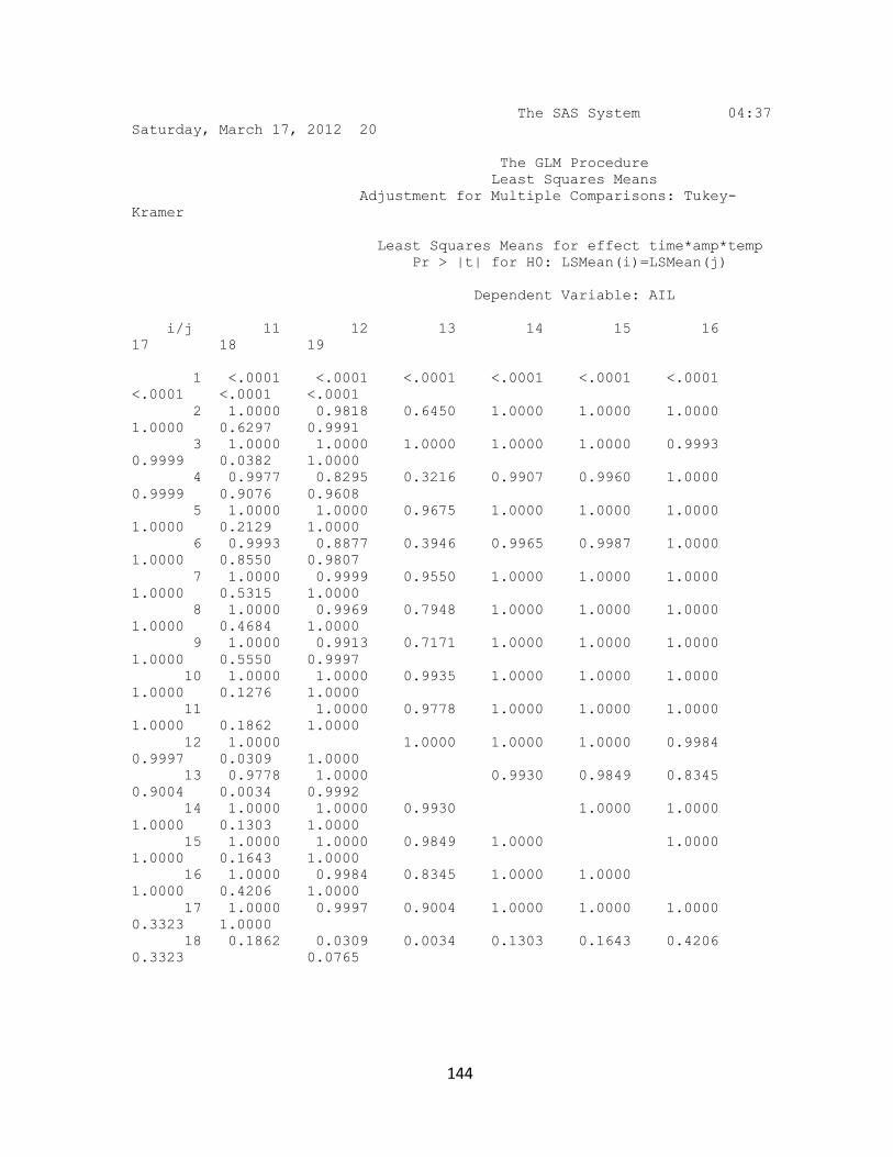
144
The SAS System 04:37
Saturday, March 17, 2012 20
The GLM Procedure
Least Squares Means
Adjustment for Multiple Comparisons: Tukey-
Kramer
Least Squares Means for effect time*amp*temp
Pr > |t| for H0: LSMean(i)=LSMean(j)
Dependent Variable: AIL
i/j 11 12 13 14 15 16
17 18 19
1 <.0001 <.0001 <.0001 <.0001 <.0001 <.0001
<.0001 <.0001 <.0001
2 1.0000 0.9818 0.6450 1.0000 1.0000 1.0000
1.0000 0.6297 0.9991
3 1.0000 1.0000 1.0000 1.0000 1.0000 0.9993
0.9999 0.0382 1.0000
4 0.9977 0.8295 0.3216 0.9907 0.9960 1.0000
0.9999 0.9076 0.9608
5 1.0000 1.0000 0.9675 1.0000 1.0000 1.0000
1.0000 0.2129 1.0000
6 0.9993 0.8877 0.3946 0.9965 0.9987 1.0000
1.0000 0.8550 0.9807
7 1.0000 0.9999 0.9550 1.0000 1.0000 1.0000
1.0000 0.5315 1.0000
8 1.0000 0.9969 0.7948 1.0000 1.0000 1.0000
1.0000 0.4684 1.0000
9 1.0000 0.9913 0.7171 1.0000 1.0000 1.0000
1.0000 0.5550 0.9997
10 1.0000 1.0000 0.9935 1.0000 1.0000 1.0000
1.0000 0.1276 1.0000
11 1.0000 0.9778 1.0000 1.0000 1.0000
1.0000 0.1862 1.0000
12 1.0000 1.0000 1.0000 1.0000 0.9984
0.9997 0.0309 1.0000
13 0.9778 1.0000 0.9930 0.9849 0.8345
0.9004 0.0034 0.9992
14 1.0000 1.0000 0.9930 1.0000 1.0000
1.0000 0.1303 1.0000
15 1.0000 1.0000 0.9849 1.0000 1.0000
1.0000 0.1643 1.0000
16 1.0000 0.9984 0.8345 1.0000 1.0000
1.0000 0.4206 1.0000
17 1.0000 0.9997 0.9004 1.0000 1.0000 1.0000
0.3323 1.0000
18 0.1862 0.0309 0.0034 0.1303 0.1643 0.4206
0.3323 0.0765
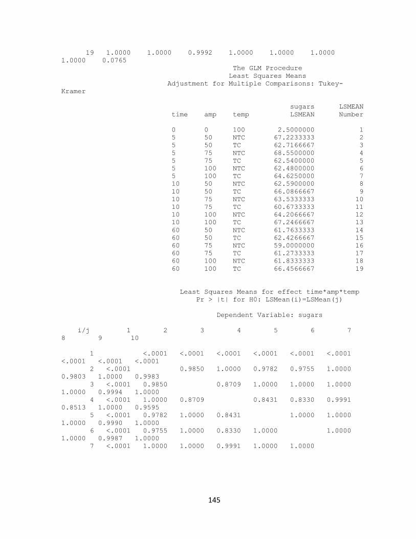
145
19 1.0000 1.0000 0.9992 1.0000 1.0000 1.0000
1.0000 0.0765
The GLM Procedure
Least Squares Means
Adjustment for Multiple Comparisons: Tukey-
Kramer
sugars LSMEAN
time amp temp LSMEAN Number
0 0 100 2.5000000 1
5 50 NTC 67.2233333 2
5 50 TC 62.7166667 3
5 75 NTC 68.5500000 4
5 75 TC 62.5400000 5
5 100 NTC 62.4800000 6
5 100 TC 64.6250000 7
10 50 NTC 62.5900000 8
10 50 TC 66.0866667 9
10 75 NTC 63.5333333 10
10 75 TC 60.6733333 11
10 100 NTC 64.2066667 12
10 100 TC 67.2466667 13
60 50 NTC 61.7633333 14
60 50 TC 62.4266667 15
60 75 NTC 59.0000000 16
60 75 TC 61.2733333 17
60 100 NTC 61.8333333 18
60 100 TC 66.4566667 19
Least Squares Means for effect time*amp*temp
Pr > |t| for H0: LSMean(i)=LSMean(j)
Dependent Variable: sugars
i/j 1 2 3 4 5 6 7
8 9 10
1 <.0001 <.0001 <.0001 <.0001 <.0001 <.0001
<.0001 <.0001 <.0001
2 <.0001 0.9850 1.0000 0.9782 0.9755 1.0000
0.9803 1.0000 0.9983
3 <.0001 0.9850 0.8709 1.0000 1.0000 1.0000
1.0000 0.9994 1.0000
4 <.0001 1.0000 0.8709 0.8431 0.8330 0.9991
0.8513 1.0000 0.9595
5 <.0001 0.9782 1.0000 0.8431 1.0000 1.0000
1.0000 0.9990 1.0000
6 <.0001 0.9755 1.0000 0.8330 1.0000 1.0000
1.0000 0.9987 1.0000
7 <.0001 1.0000 1.0000 0.9991 1.0000 1.0000
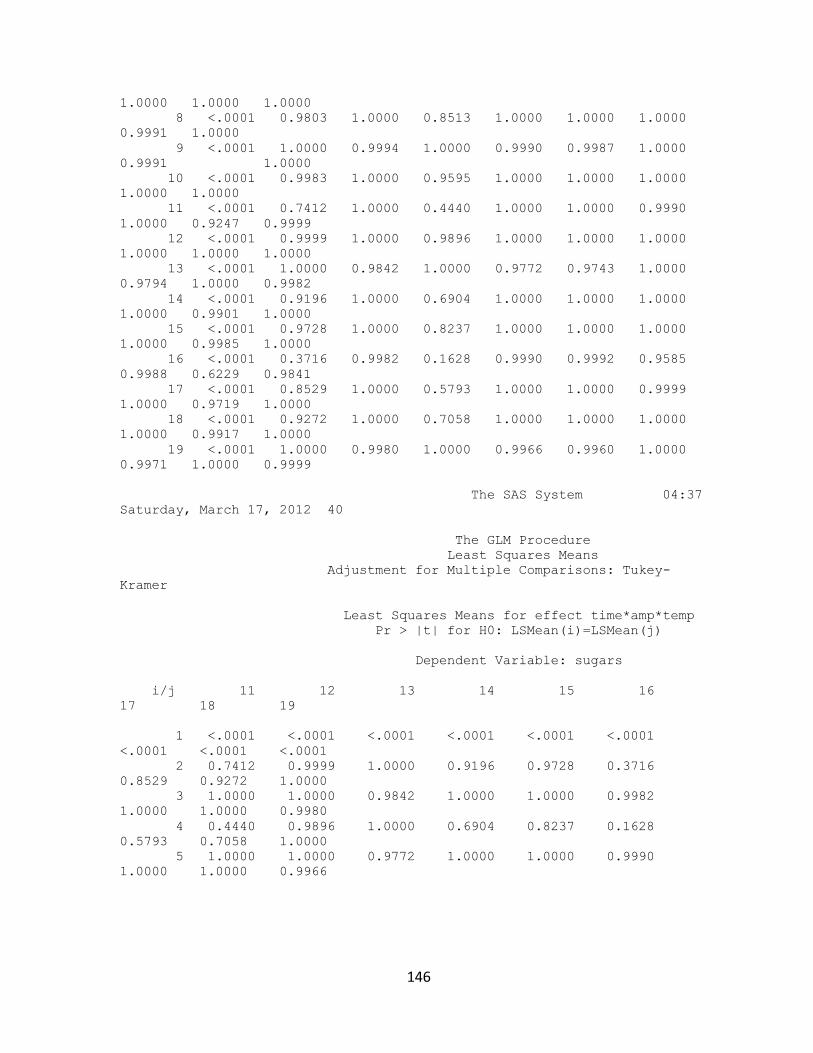
146
1.0000 1.0000 1.0000
8 <.0001 0.9803 1.0000 0.8513 1.0000 1.0000 1.0000
0.9991 1.0000
9 <.0001 1.0000 0.9994 1.0000 0.9990 0.9987 1.0000
0.9991 1.0000
10 <.0001 0.9983 1.0000 0.9595 1.0000 1.0000 1.0000
1.0000 1.0000
11 <.0001 0.7412 1.0000 0.4440 1.0000 1.0000 0.9990
1.0000 0.9247 0.9999
12 <.0001 0.9999 1.0000 0.9896 1.0000 1.0000 1.0000
1.0000 1.0000 1.0000
13 <.0001 1.0000 0.9842 1.0000 0.9772 0.9743 1.0000
0.9794 1.0000 0.9982
14 <.0001 0.9196 1.0000 0.6904 1.0000 1.0000 1.0000
1.0000 0.9901 1.0000
15 <.0001 0.9728 1.0000 0.8237 1.0000 1.0000 1.0000
1.0000 0.9985 1.0000
16 <.0001 0.3716 0.9982 0.1628 0.9990 0.9992 0.9585
0.9988 0.6229 0.9841
17 <.0001 0.8529 1.0000 0.5793 1.0000 1.0000 0.9999
1.0000 0.9719 1.0000
18 <.0001 0.9272 1.0000 0.7058 1.0000 1.0000 1.0000
1.0000 0.9917 1.0000
19 <.0001 1.0000 0.9980 1.0000 0.9966 0.9960 1.0000
0.9971 1.0000 0.9999
The SAS System 04:37
Saturday, March 17, 2012 40
The GLM Procedure
Least Squares Means
Adjustment for Multiple Comparisons: Tukey-
Kramer
Least Squares Means for effect time*amp*temp
Pr > |t| for H0: LSMean(i)=LSMean(j)
Dependent Variable: sugars
i/j 11 12 13 14 15 16
17 18 19
1 <.0001 <.0001 <.0001 <.0001 <.0001 <.0001
<.0001 <.0001 <.0001
2 0.7412 0.9999 1.0000 0.9196 0.9728 0.3716
0.8529 0.9272 1.0000
3 1.0000 1.0000 0.9842 1.0000 1.0000 0.9982
1.0000 1.0000 0.9980
4 0.4440 0.9896 1.0000 0.6904 0.8237 0.1628
0.5793 0.7058 1.0000
5 1.0000 1.0000 0.9772 1.0000 1.0000 0.9990
1.0000 1.0000 0.9966
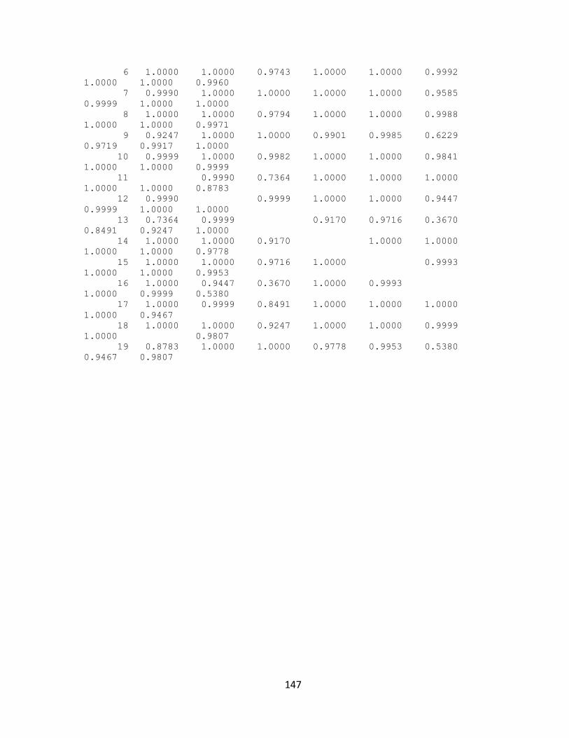
147
6 1.0000 1.0000 0.9743 1.0000 1.0000 0.9992
1.0000 1.0000 0.9960
7 0.9990 1.0000 1.0000 1.0000 1.0000 0.9585
0.9999 1.0000 1.0000
8 1.0000 1.0000 0.9794 1.0000 1.0000 0.9988
1.0000 1.0000 0.9971
9 0.9247 1.0000 1.0000 0.9901 0.9985 0.6229
0.9719 0.9917 1.0000
10 0.9999 1.0000 0.9982 1.0000 1.0000 0.9841
1.0000 1.0000 0.9999
11 0.9990 0.7364 1.0000 1.0000 1.0000
1.0000 1.0000 0.8783
12 0.9990 0.9999 1.0000 1.0000 0.9447
0.9999 1.0000 1.0000
13 0.7364 0.9999 0.9170 0.9716 0.3670
0.8491 0.9247 1.0000
14 1.0000 1.0000 0.9170 1.0000 1.0000
1.0000 1.0000 0.9778
15 1.0000 1.0000 0.9716 1.0000 0.9993
1.0000 1.0000 0.9953
16 1.0000 0.9447 0.3670 1.0000 0.9993
1.0000 0.9999 0.5380
17 1.0000 0.9999 0.8491 1.0000 1.0000 1.0000
1.0000 0.9467
18 1.0000 1.0000 0.9247 1.0000 1.0000 0.9999
1.0000 0.9807
19 0.8783 1.0000 1.0000 0.9778 0.9953 0.5380
0.9467 0.9807
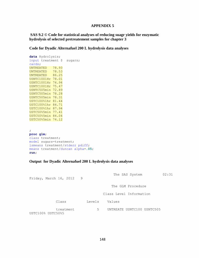
148
APPENDIX 5
SAS 9.2 © Code for statistical analyses of reducing suagr yields for enzymatic
hydrolysis of selected pretreatement samples for chapter 3
Code for Dyadic Alternafuel 200 L hydrolysis data analyses
data Hydrolysis;
input treatment $ sugars;
cards;
UNTREATED 78.93
UNTREATED 78.53
UNTREATED 86.25
USNTC1001Hr 78.01
USNTC1001Hr 74.94
USNTC1001Hr 75.47
USNTC505min 72.89
USNTC505min 78.28
USNTC505min 78.31
USTC100%1hr 81.44
USTC100%1hr 84.71
USTC100%1hr 87.94
USTC50%5min 77.41
USTC50%5min 84.04
USTC50%5min 74.12
;
proc glm;
class treatment;
model sugars=treatment;
lsmeans treatment/stderr pdiff;
means treatment/duncan alpha=.05;
run;
Output for Dyadic Alternafuel 200 L hydrolysis data analyses
The SAS System 02:31
Friday, March 16, 2012 9
The GLM Procedure
Class Level Information
Class Levels Values
treatment 5 UNTREATE USNTC100 USNTC505
USTC100% USTC50%5
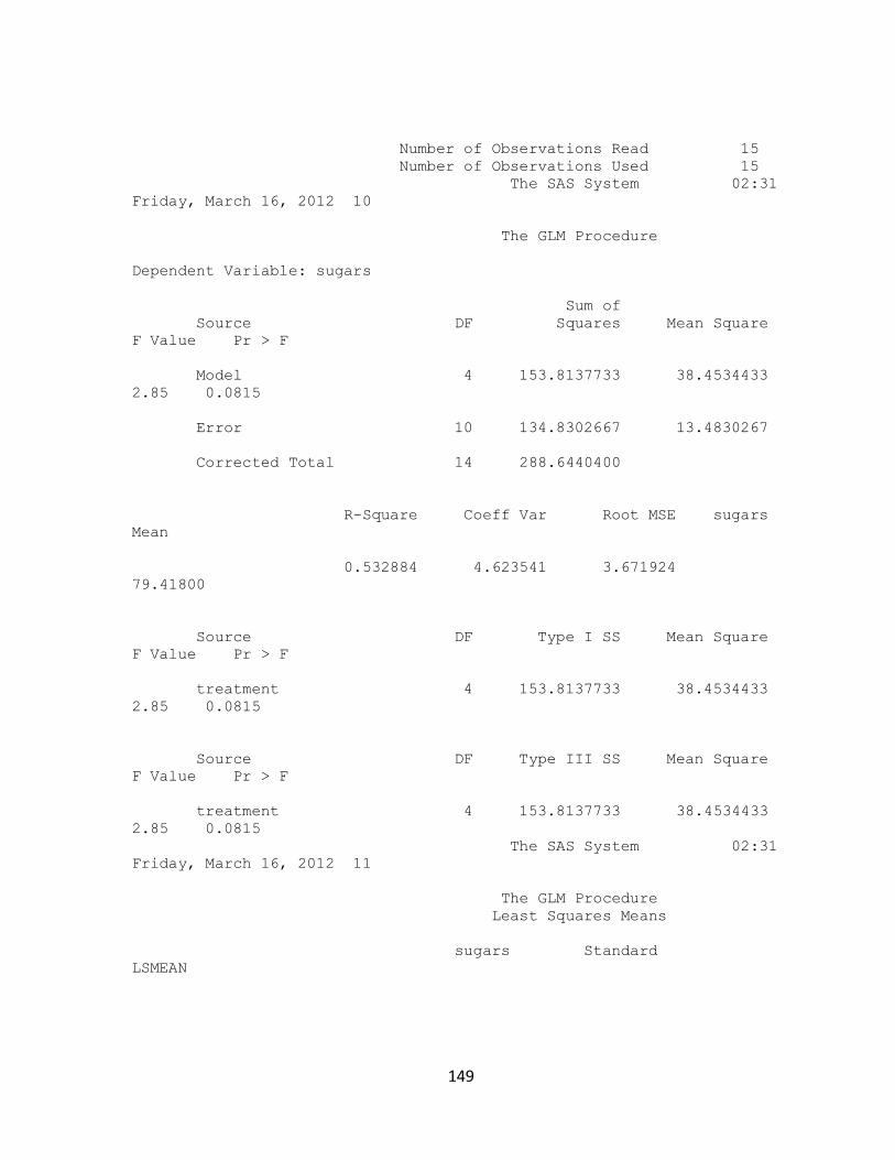
149
Number of Observations Read 15
Number of Observations Used 15
The SAS System 02:31
Friday, March 16, 2012 10
The GLM Procedure
Dependent Variable: sugars
Sum of
Source DF Squares Mean Square
F Value Pr > F
Model 4 153.8137733 38.4534433
2.85 0.0815
Error 10 134.8302667 13.4830267
Corrected Total 14 288.6440400
R-Square Coeff Var Root MSE sugars
Mean
0.532884 4.623541 3.671924
79.41800
Source DF Type I SS Mean Square
F Value Pr > F
treatment 4 153.8137733 38.4534433
2.85 0.0815
Source DF Type III SS Mean Square
F Value Pr > F
treatment 4 153.8137733 38.4534433
2.85 0.0815
The SAS System 02:31
Friday, March 16, 2012 11
The GLM Procedure
Least Squares Means
sugars Standard
LSMEAN
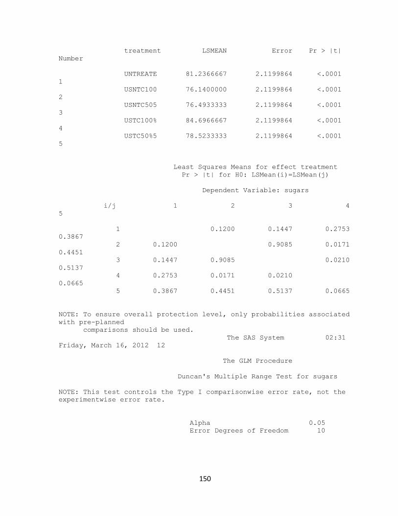
150
treatment LSMEAN Error Pr > |t|
Number
UNTREATE 81.2366667 2.1199864 <.0001
1
USNTC100 76.1400000 2.1199864 <.0001
2
USNTC505 76.4933333 2.1199864 <.0001
3
USTC100% 84.6966667 2.1199864 <.0001
4
USTC50%5 78.5233333 2.1199864 <.0001
5
Least Squares Means for effect treatment
Pr > |t| for H0: LSMean(i)=LSMean(j)
Dependent Variable: sugars
i/j 1 2 3 4
5
1 0.1200 0.1447 0.2753
0.3867
2 0.1200 0.9085 0.0171
0.4451
3 0.1447 0.9085 0.0210
0.5137
4 0.2753 0.0171 0.0210
0.0665
5 0.3867 0.4451 0.5137 0.0665
NOTE: To ensure overall protection level, only probabilities associated
with pre-planned
comparisons should be used.
The SAS System 02:31
Friday, March 16, 2012 12
The GLM Procedure
Duncan's Multiple Range Test for sugars
NOTE: This test controls the Type I comparisonwise error rate, not the
experimentwise error rate.
Alpha 0.05
Error Degrees of Freedom 10
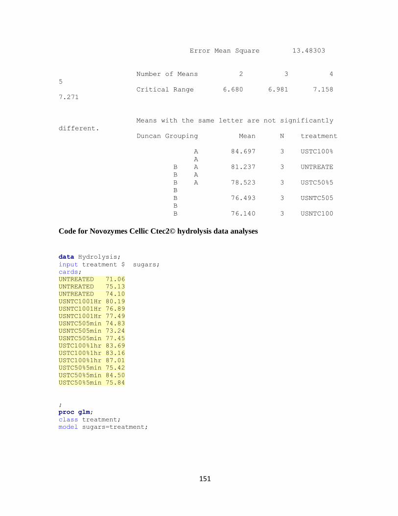
151
Error Mean Square 13.48303
Number of Means 2 3 4
5
Critical Range 6.680 6.981 7.158
7.271
Means with the same letter are not significantly
different.
Duncan Grouping Mean N treatment
A 84.697 3 USTC100%
A
B A 81.237 3 UNTREATE
B A
B A 78.523 3 USTC50%5
B
B 76.493 3 USNTC505
B
B 76.140 3 USNTC100
Code for Novozymes Cellic Ctec2© hydrolysis data analyses
data Hydrolysis;
input treatment $ sugars;
cards;
UNTREATED 71.06
UNTREATED 75.13
UNTREATED 74.10
USNTC1001Hr 80.19
USNTC1001Hr 76.89
USNTC1001Hr 77.49
USNTC505min 74.83
USNTC505min 73.24
USNTC505min 77.45
USTC100%1hr 83.69
USTC100%1hr 83.16
USTC100%1hr 87.01
USTC50%5min 75.42
USTC50%5min 84.50
USTC50%5min 75.84
;
proc glm;
class treatment;
model sugars=treatment;
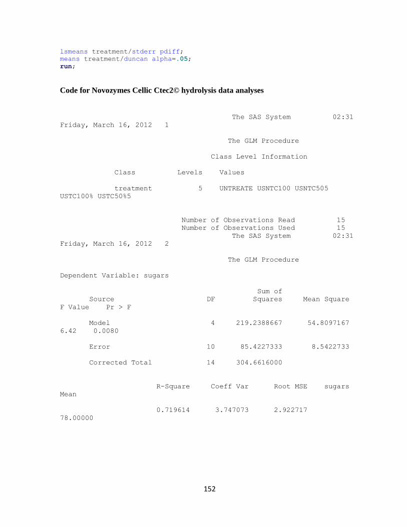
152
lsmeans treatment/stderr pdiff;
means treatment/duncan alpha=.05;
run;
Code for Novozymes Cellic Ctec2© hydrolysis data analyses
The SAS System 02:31
Friday, March 16, 2012 1
The GLM Procedure
Class Level Information
Class Levels Values
treatment 5 UNTREATE USNTC100 USNTC505
USTC100% USTC50%5
Number of Observations Read 15
Number of Observations Used 15
The SAS System 02:31
Friday, March 16, 2012 2
The GLM Procedure
Dependent Variable: sugars
Sum of
Source DF Squares Mean Square
F Value Pr > F
Model 4 219.2388667 54.8097167
6.42 0.0080
Error 10 85.4227333 8.5422733
Corrected Total 14 304.6616000
R-Square Coeff Var Root MSE sugars
Mean
0.719614 3.747073 2.922717
78.00000
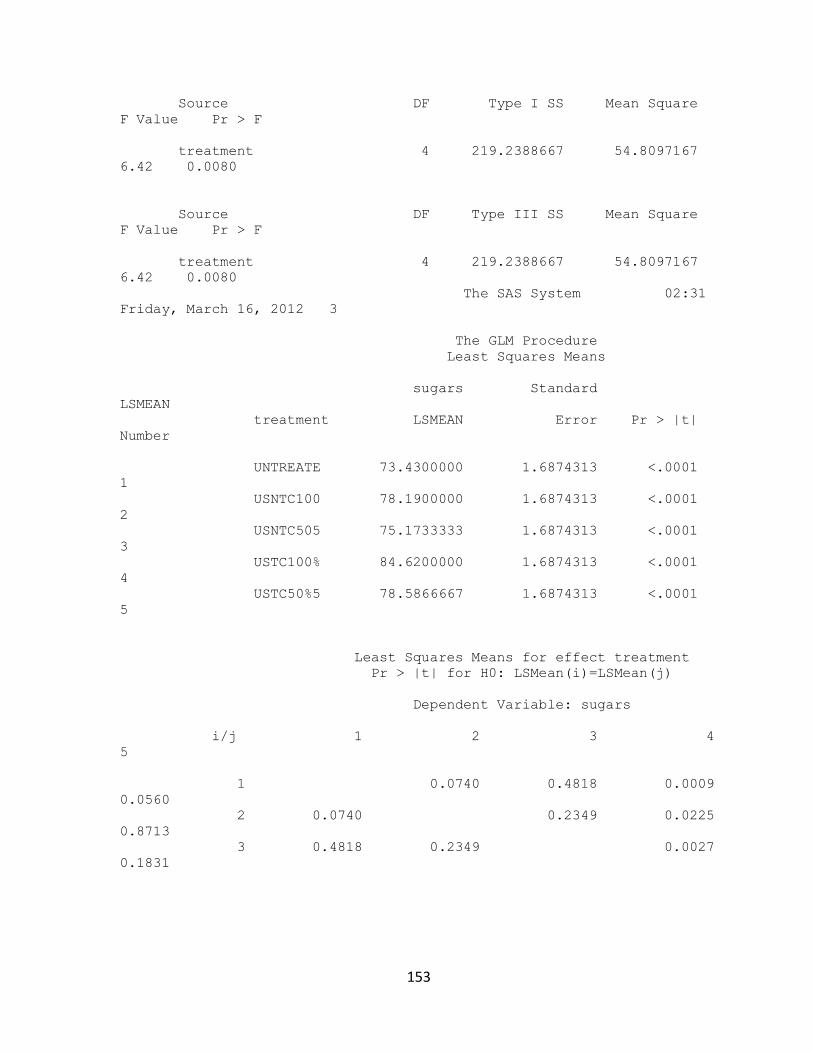
153
Source DF Type I SS Mean Square
F Value Pr > F
treatment 4 219.2388667 54.8097167
6.42 0.0080
Source DF Type III SS Mean Square
F Value Pr > F
treatment 4 219.2388667 54.8097167
6.42 0.0080
The SAS System 02:31
Friday, March 16, 2012 3
The GLM Procedure
Least Squares Means
sugars Standard
LSMEAN
treatment LSMEAN Error Pr > |t|
Number
UNTREATE 73.4300000 1.6874313 <.0001
1
USNTC100 78.1900000 1.6874313 <.0001
2
USNTC505 75.1733333 1.6874313 <.0001
3
USTC100% 84.6200000 1.6874313 <.0001
4
USTC50%5 78.5866667 1.6874313 <.0001
5
Least Squares Means for effect treatment
Pr > |t| for H0: LSMean(i)=LSMean(j)
Dependent Variable: sugars
i/j 1 2 3 4
5
1 0.0740 0.4818 0.0009
0.0560
2 0.0740 0.2349 0.0225
0.8713
3 0.4818 0.2349 0.0027
0.1831
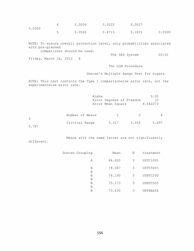
154
4 0.0009 0.0225 0.0027
0.0300
5 0.0560 0.8713 0.1831 0.0300
NOTE: To ensure overall protection level, only probabilities associated
with pre-planned
comparisons should be used.
The SAS System 02:31
Friday, March 16, 2012 4
The GLM Procedure
Duncan's Multiple Range Test for sugars
NOTE: This test controls the Type I comparisonwise error rate, not the
experimentwise error rate.
Alpha 0.05
Error Degrees of Freedom 10
Error Mean Square 8.542273
Number of Means 2 3 4
5
Critical Range 5.317 5.556 5.697
5.787
Means with the same letter are not significantly
different.
Duncan Grouping Mean N treatment
A 84.620 3 USTC100%
B 78.587 3 USTC50%5
B
B 78.190 3 USNTC100
B
B 75.173 3 USNTC505
B
B 73.430 3 UNTREATE


