

Journal of Computational Physics 214 (2006) 633–656
www.elsevier.com/locate/jcp
Accelerating the convergence of spectral deferredcorrection methods
Jingfang Huang *, Jun Jia, Michael Minion
Department of Mathematics, University of North Carolina, CB#3250, Philips Hall, Chapel Hill, North Carolina 27599, USA
Received 9 May 2005; received in revised form 6 October 2005; accepted 7 October 2005Available online 29 November 2005
Abstract
In the recent paper by Dutt, Greengard and Rokhlin, a variant of deferred or defect correction methods is presentedwhich couples Gaussian quadrature with the Picard integral equation formulation of the initial value ordinary differentialequation. The resulting spectral deferred correction (SDC) methods have been shown to possess favorable accuracy andstability properties even for versions with very high order of accuracy. In this paper, we show that for linear problems,the iterations in the SDC algorithm are equivalent to constructing a preconditioned Neumann series expansion for thesolution of the standard collocation discretization of the ODE. This observation is used to accelerate the convergenceof SDC using the GMRES Krylov subspace method. For nonlinear problems, the GMRES acceleration is coupled witha linear implicit approach. Stability and accuracy analyses show the accelerated scheme provides an improvement in theaccuracy, efficiency, and stability of the original SDC approach. Furthermore, preliminary numerical experiments showthat accelerating the convergence of SDC methods can effectively eliminate the order reduction previously observed forstiff ODE systems.� 2005 Elsevier Inc. All rights reserved.
MSC: 65B05; 65F10; 65L05
Keywords: Spectral deferred correction methods; Stiff equations; Krylov subspace methods; GMRES
1. Introduction
Inprobl
tion h
0021-9
doi:10.
* CoE-m
this paper, we discuss the numerical solution of the ordinary differential equation (ODE) initial valueem
u0ðtÞ ¼ F ðt;uðtÞÞ; t 2 ½0; T �; ð1Þ
uð0Þ ¼ u0; ð2Þwhere u ;uðtÞ 2 CN and F : R� CN ! CN . Many numerical techniques for approximating this type of equa-
0ave been developed in the last century and the readers are referred to [3,4,10,15,16,23,32] for detailed
991/$ - see front matter � 2005 Elsevier Inc. All rights reserved.
1016/j.jcp.2005.10.004
rresponding author. Fax: +1 919 962 9345.ail addresses: [email protected] (J. Huang), [email protected] (J. Jia), [email protected] (M. Minion).

discussions. In this paper, we present a technique which is designed to improve the performance of the spectraldeferred correction (SDC) methods introduced by Dutt, Greengard, and Rokhlin in 2000 [9]. The SDC strat-egy introduced in [9] is a variation on the classical defect or deferred correction methods [5,25,28,31,34,35]which allows for the construction of stable explicit and implicit methods with extremely high order of accu-racy. As with classical deferred and defect correction methods cited above, a single time step of an SDC meth-od begins by first dividing the time step [tn, tn+1] into a set of intermediate sub-steps defined by the points~t ¼ ½t0; t1; . . . ; tp� with tn = t0 < t1 < . . . < tp 6 tn+1. For simplicity, we assume tn = t0 = 0 in the following dis-cussions. Next, a provisional approximation ~u½0� ¼ ½u½0�ðt0Þ;u½0�ðt1Þ; � � � ;u½0�ðtpÞ� is computed at the intermedi-ate points using a standard numerical method, e.g., the explicit Euler method for non-stiff problems or theimplicit Euler method for stiff problems as in [9]. Applying standard approximation or interpolation theory,the continuous counter part of ~u½0� can be constructed and is represented as u[0](t). Using u[0](t), an equationfor the error d(t) = u(t)�u[0](t) is then constructed. This correction equation for d(t) can be approximatedusing a similar low order method, and an improved numerical solution is constructed. This procedure can thenbe repeated resulting in a sequence of approximate solutions.
To construct the correction equation, the classical methods cited above rely on differentiation of u[0](t) toform an ODE for d(t), where u[0](t) is the interpolating polynomial of ~u½0�. On the other hand, SDC methods
634 J. Huang et al. / Journal of Computational Physics 214 (2006) 633–656
utiliz
to co
wher
vergesolut
e the Picard integral equation formulation of the ODEZ t
uðtÞ ¼ u0 þ0
F ðs;uðsÞÞds ð3Þ
nstruct a corresponding integral equation for d(t). SpecificallyZ t
dðtÞ ¼0
½F ðs;u½0�ðsÞ þ dðsÞÞ � F ðs;u½0�ðsÞÞ�dsþ �ðtÞ; ð4Þ
e Z t
�ðtÞ ¼ u0 þ0
F ðs;u½0�ðsÞÞds� u½0�ðtÞ. ð5Þ
The discretizaton of these equations will be discussed in more detail in the following section, but for now notethat the discretization of �(t) is simply a numerical integration. It is for this reason that the points~t which de-fine the sub-steps in SDC methods are chosen to be Gaussian quadrature nodes so the numerically stable spec-tral integration technique can be applied [12]. The integral equation formulation for d(t) in Eq. (4) coupledwith spectral integration rules allows SDC methods to overcome the loss of stability of classical deferred/de-fect correction methods as the order of the method increases. For a detailed discussion of the different choicesof quadrature nodes see [24].
Deferred correction methods based on the Picard integral formulation and spectral integration are of inter-est for several reasons, most notably because of the relative ease with which one can theoretically constructmethods with arbitrarily high order of accuracy. Preliminary numerical tests presented in [9] suggest thatSDC methods are competitive with the best existing ODE initial value problem solvers, especially for stiffproblems or where high accuracy is required. Furthermore the stability regions of the implicit methods areclose to optimal and do not degrade with increased orders of accuracy [24]. Semi-implicit and multi-implicitvariations of SDC methods have also been presented which enable the construction of very high order meth-ods for equations with both stiff and non-stiff components [6,26,27]. Also noted in these papers, however, isthe fact that when SDC methods are applied to very stiff equations, the effective order of accuracy of themethod is reduced for values of the time step above a certain threshold. This type of order reduction (whichis also present in many popular types of Runge–Kutta methods [7,8,30]) means that, although the methods arestable for larger time steps, one must use a very small time step for the method to converge with full order.
The main results in this paper stem from considering the limit of the correction iterations for an SDCmethod for a fixed step of size Dt = tn+1 � tn. Observe that, if the correction iteration in the SDC method con-
~
s, then �(t) given in Eq. (5) will approach zero at the Gaussian nodes t 2 ½t ; t �. Hence the resulting limit n nþ1ion will satisfy the collocation (or pseudo-spectral) approximation of the Picard equation (3) given by
~u ¼ ~u0 þ DtS~F ; ð6Þ

J. Huang et al. / Journal of Computational Physics 214 (2006) 633–656 635
where
~u0 is
condisoluti
accur
CoSupp
~F ¼ ½F ðt0;uðt0ÞÞ; F ðt1;uðt1ÞÞ; . . . ; F ðtp;uðtpÞÞ�T;
a vector of initial conditions~u0 ¼ ½uðt0Þ;uðt0Þ; . . . ;uðt0Þ�T
and S is the spectral integration matrix [11,12] corresponding to the Gaussian nodes~t discussed in detail inSection 2.3.
Since Eq. (6) couples the solution values at each of the sub-steps defined by~t, a direct solution of this equa-tion requires a system of size Np be solved, as opposed to a system of size N which arises from a single sub-stepof an SDC method (or in other typical methods like BDF). However, since the limit of the SDC iterations(when it converges) is the collocation solution, then one iteration of the correction step in an SDC methodcan also be thought of as one step in an iterative procedure for solving Eq. (6) directly. Once this observationis made, it is natural to attempt to accelerate this convergence if possible.
In Section 3, we show that for linear problems, the SDC method is equivalent to solving a particular pre-
tioned equation for the error corresponding to Eq. (6). Moreover, an explicit form for the provisionalon after the kth SDC iteration ~u½k� in terms of a Neumann series expansion is derived. Specifically,~u½k� �~u½0� �~bþ C~bþ C2~bþ � � � þ Ck~b ð7Þfor a specific matrix C and vector ~b. A consequence of the derivation of Eq. (7) is that it provides a precisestatement of when and how rapidly the correction iterations in the SDC method converge. This observationcan also be used to accelerate the convergence of the original SDC methods by searching for the optimal solu-tion in the Krylov subspace KðC;~bÞ ¼ spanf~b;C~b;C2~b; . . . ;Ck~bg using the generalized minimum residual(GMRES) or other Krylov subspace based iterative methods. For nonlinear problems, the above accelerationcan be coupled with a linear implicit approach to improve the performance of SDC methods.
In this paper, the new class of accelerated methods is studied analytically and numerical comparisons withthe original SDC methods for both linear and nonlinear problems are presented. Stability and accuracy anal-yses for the accelerated schemes are given. We observe that for non-stiff problems, GMRES accelerated SDCmethods improve both the accuracy and stability of the original SDC methods. In fact, in several numericalexamples we tested, for a given time step of size Dt, the accelerated methods quickly converge to the colloca-tion solution while the correction iterations of the original SDC are divergent. For stiff problems [20], we showthe accelerated methods improve the accuracy of the original SDC, and under certain assumptions, remove theorder reduction phenomenon observed in the original SDC.
The structure of this paper is as follows. In Section 2, we briefly describe the original spectral deferred cor-rection methods. In Section 3, we show that for linear problems, the original SDC is equivalent to the precon-ditioned Neumann series expansion given in Eq. (7). In Section 4, we describe how the convergence of theoriginal SDC can be accelerated for both linear and non-linear problems. In Section 5, we present the stabilityand accuracy analyses for the GMRES accelerated SDC methods. In Section 6, we demonstrate the improved
acy and stability of the accelerated methods using several linear and nonlinear examples. Finally in Sec-
tion 7, we discuss possible extensions and further generalizations of the approach.2. The spectral deferred correction methods
In this section, we summarize the details of the spectral deferred correction methods from [9] which are nec-essary to present the derivation of the accelerated methods in Sections 3 and 4.
2.1. The Picard integral equation and error equation
nsider the Picard integral equation representation of the ODE initial value problem given in Eq. (3).ose an approximate solution u[0](t) to Eqs. (1) and (2) is given, and define the error d(t) as before
dðtÞ ¼ uðtÞ � u½0�ðtÞ. ð8Þ

636 J. Huang et al. / Journal of Computational Physics 214 (2006) 633–656
Subst
impli
whichtype
improstep i
Note
Lettinof Eq
wher
polatto th
ituting (8) into (3) yieldsZ t
u½0�ðtÞ þ dðtÞ ¼ u0 þ0
F ðs;u½0�ðsÞ þ dðsÞÞds. ð9Þ
To reduce notational clutter here and in the following the time dependence of the second argument of F will be
citly assumed, e.g., F(t,u[0](t)) is written simply as F(t,u[0]). Now consider the residual functionZ t�ðtÞ ¼ u0 þ0
F ðs;u½0�Þds� u½0�ðtÞ; ð10Þ
simply gives the error in the Picard equation (3). Rearranging Eq. (9) and using Eq. (10) gives a Picard-
integral equation for the errorZ tdðtÞ ¼0
½F ðs;u½0� þ dÞ � F ðs;u½0�Þ�dsþ �ðtÞ. ð11Þ
Note that unlike the classical deferred or defect correction methods in [28,34,35], the equation for d(t) is notwritten here as an ODE.
2.2. Euler methods on Gaussian quadrature nodes
Deferred correction methods proceed by iteratively solving the error Eq. (11) using a low order method to½0�
ve the provisional solution ~u . To describe the time stepping procedure, suppose as before that the timenterval [tn, tn+1] has been subdivided using the points t0,t1,t2, . . ., tp such that
tn ¼ t0 < t1 < t2 � � � < tp 6 tnþ1. ð12Þ
that Eq. (11) gives the identityZ tmþ1½0� ½0�
dðtmþ1Þ ¼ dðtmÞ þtm½F ðs;u þ dÞ � F ðs;u Þ�dsþ �ðtmþ1Þ � �ðtmÞ. ð13Þ
½0�
g dm denote the numerical approximation to d(tm) (and likewise for um and �m), a simple discretization. (13) similar to the explicit Euler (forward Euler) method for ODEs isdmþ1 ¼ dm þ DtmðF ðtm;u½0�m þ dmÞ � F ðtm;u
½0�m ÞÞ þ �mþ1 � �m; ð14Þ
e Dtm = tm+1�tm. Similarly, an implicit scheme for the solution based on the backward Euler method is� �
dmþ1 ¼ dm þ Dtm F ðtmþ1;u½0�mþ1 þ dmþ1Þ � F ðtmþ1;u
½0�mþ1Þ þ �mþ1 � �m. ð15Þ
Denoting the ‘‘low order’’ approximation of d(t) by ~d½1�¼ ½d1; d2; . . . ; dp�, a refined solution is given by
~u½1� ¼ ~u½0� þ~d½1�
. In order to complete the discretization, we must specify how the terms �m are computed.
2.3. The spectral integration matrix
First note that there are various ways to choose the points t0,t1,t2, . . ., tp to define the sub-steps in the SDCmethod. When Gaussian quadrature nodes are used, {t1, . . .tp} are interior points in [tn, tn+1] and the endpointsare not used. On the other hand the Radau Ia quadrature nodes t0,t1,t2, . . ., tp use the left end point while theRadau IIa nodes t1,t2, . . ., tp have tp = tn+1. Finally, the Lobatto quadrature rule requires the use of both endpoints.
Using the Gaussian nodes as an example, suppose we are given the scalar function values~u ¼ fu1;u2; . . . ;upg at the nodes, then the Legendre polynomial expansion Lpð~u; tÞ can be constructed toapproximate ~u where the coefficients are computed using Gaussian quadrature rules. This gives a numericallystable and efficient way to find the equivalent interpolating polynomial of degree p � 1. Integrating this inter-
ing polynomial analytically from t0 to tm, a linear mapping Q is derived which maps the function values ~ue integral of the interpolating polynomial
case wlength
choic
the in
Co
Rema
has a
Z tm
J. Huang et al. / Journal of Computational Physics 214 (2006) 633–656 637
½~u�m ¼t0
Lpð~u; sÞds.
can be written in matrix form
ThisQ~u ¼ DtS~u; ð16Þwhere S will be referred to as the integration matrix, and is independent of Dt. Note that in the more general
N ~ ~
here uðtÞ 2 C , Eq. (16) must be interpreted as being applied component-wise to u, i.e., u is a vector ofNp andQ~u ¼ DtðIp � SÞ~u; ð17Þwhere Ip is the identity matrix of size p · p. In the following, we use script font to denote this tensor product,i.e. S denotes the Np · Np block diagonal matrix Ip � S.
For traditional deferred/defect correction methods, there are two factors which prevent the use of extremelyhigh order methods: The first problem relates to the instability of interpolation at equispaced nodes where theRunge phenomenon can be observed when the number of interpolation points p is large. The second problemis that numerical differentiation in the original ODE formulation (Eqs. (1) and (2)) introduces instabilities [33].Spectral deferred correction methods avoid both of these difficulties by introducing Gaussian-type nodes andusing the Picard integral equation. The procedure is explained in next section. In the current numerical imple-mentation, the Legendre polynomial based Radau IIa quadrature nodes are used and the matrix S is precom-puted using Mathematica requesting more than 20 digits in accuracy. Detailed comparisons of different
es of nodes will be reported in the future (see also [24]).
2.4. The spectral deferred correction algorithm
Given an approximate solution ~u½0� ¼ ½u½0�; . . . ;u½0��, consider the error equation given by (11). Discretizing
1 ptegral in (10) in the same manner as in (6) using the spectral integration matrix yields
~� ¼ ~u0 þ DtS~F �~u½0�; ð18Þwhere~� ¼ ½�ðt1Þ; . . . ; �ðtpÞ� is the residual at the intermediate points. Once the residual is calculated, an approx-
imation~d½1�
to the error Eq. (11) is computed using p steps of the Eq. (14) for non-stiff problems or Eq. (15) for
stiff problems. The provisional solution is then updated with ~u½1� ¼ ~u½0� þ~d½1�
, and this procedure can be re-peated. The algorithm for SDC is given by the following:
Pseudo-code: spectral deferred correction method
Comment [Compute initial approximation]For non-stiff/stiff problems, use the forward/backward Euler method to compute an approximate solu-
tion u½0� � uðt Þ at the sub-steps t , . . ., t on the interval [t , t ].
m m 1 p n n+1mment [Compute successive corrections.]
do j =rk 2.
lso be
1, . . .,J
(1) Compute the approximate residual function~� using ~u½j�1� and Eq. (18).
(2a) For non-stiff problems, compute ~d½j�
using p steps of Eq. (14).
(2b) For stiff problems, compute ~d½j�
using p steps of Eq. (15).
(3) Update the approximate solution ~u½j� ¼ ~u½j�1� þ~d½j�
.
endoIt can be shown that each correction procedure in this algorithm can improve the order of the method by one,as long as such improvement has not gone beyond the degree of the underlying interpolating polynomial andthe quadrature rules [13,18,19]. For linear ODE problems, a proof is provided in Section 3.2 utilizing the Neu-mann series expansion.
1. For the initial approximation, an alternative method is to use a constant approximation. Thisen implemented and tested. Detailed analysis and comparisons will be reported in the future.

2.5. The collocation formulation limit of SDC
638 J. Huang et al. / Journal of Computational Physics 214 (2006) 633–656
Cothen
Fou[0](t
wherappro
Filinear
Summsome
Noticthe in
There
nsider the iterative correction procedure detailed in the last section. If the SDC procedure is convergent,by Eq. (18) the limit satisfies~� ¼ 0, which is equivalent to
~u ¼ ~u0 þ DtS~F . ð19ÞThis is identical to the collocation formula given in Eq. (6). Conditions specifying precisely when the SDCconverges to this limit for linear systems are presented in Section 3.
It is possible to solve this equation directly using, for example, Newton�s method [16,17]. However, foruðtÞ 2 CN and assuming p interior points are used in each time step, the total number of unknowns in the col-location formula is M = pN. Therefore each iteration of Newton�s method (or a direct solution if the problemis linear) requires inverting a matrix of size M · M. In contrast, each correction iteration of the SDC methodrequires solving p linear or nonlinear systems with N unknowns. When the number of iterative corrections issmall, SDC methods will be more efficient compared with the direct Newton�s method approach, especiallywhen the order p is high.
3. Spectral deferred corrections in matrix form
In the previous section, we show that the SDC method can be considered as an iterative scheme for solvingthe implicit equation arising from a direct discretization of the Picard integral equation in (19). In this section,we derive an explicit representation of the iteration in matrix form for the linear case which proves that theSDC iterations converge for linear systems and aids in analyzing and accelerating the convergence.
r the present, let F(t,u(t)) = Lu(t) + f(t) where L is a constant matrix. Given an approximate solution), the discretized collocation formulation for the error equation in (11) becomes
~d� DtSL~d ¼ ~u0 þ DtS~F �~u½0�;
e L ¼ Ip � L (see Section 2.3). Denoting the right hand side by ~�, the SDC procedure iterativelyximatesðI� DtSLÞ~d ¼~� ð20Þusing the low order approximations~d
½j�for j = 1,2, . . .. The goal of this section is to rewrite SDC methods in a
matrix form and show that the original SDC technique is equivalent to solving Eq. (20) using a preconditioned
Neumann series expansion, i.e., ~d ¼P1
j¼1~d½j�
where ~d½jþ1�¼ C~d
½j�for an explicit matrix C.
3.1. Euler method in matrix form
rst consider the forward Euler method in Eq. (14) which is appropriate for non-stiff problems. For thecorrection Eq. (20), a sub-step is given by
dmþ1 ¼ dm þ DtmLdm þ ð�mþ1 � �mÞ. ð21Þ
ing successive values of d and using the fact that both the error d(t) and the residual �(t) are zero at t0,manipulation givesXmdmþ1 ¼i¼1
DtiLdi þ �mþ1. ð22ÞPm
e that i¼1DtiLdi is the composite rectangular rule approximation (where the left end point is used) oftegralZ tiþ1
0
LdðsÞds.
fore, in matrix form, the forward Euler method is equivalent to solving� �
I� DteSL ~d½1�¼~�; ð23Þ
J. Huang et al. / Journal of Computational Physics 214 (2006) 633–656 639
where
the im
colloclower
Su
Applbetwe
where
It is a
~d½1�¼ ½d1; d2; . . . dp�T,~� ¼ ½�1; �2; . . . ; �p�T, and
DteS ¼
0 0 � � � 0 0
Dt1 0 � � � 0 0
Dt1 Dt2 � � � 0 0
Dt1 Dt2 � � � 0 0
� � � � � 0 0
26666666664
37777777775
. ð24Þ
Dt1 Dt2 � � � Dtp�1 0
Notice that eS is a strictly lower triangular approximation of the spectral integration matrix S. Similarly, for
plicit Euler method, the matrix eS takes the formDteS ¼Dt0 0 � � � 0 0
Dt0 Dt1 � � � 0 0
Dt0 Dt1 � � � 0 0
� � � � � 0 0
Dt0 Dt1 � � � Dtp�2 0
2666666664
3777777775
. ð25Þ
Dt0 Dt1 � � � Dtp�2 Dtp�1
This lower triangular matrix is also an approximation of the spectral integration matrix, with non-zero diag-onal entries.
To summarize, each correction in the SDC method may be considered as solving an approximation of the
ation formulation of the correction Eq. (20), where the spectral integration matrix is approximated by a triangular matrix. Clearly, the solution given by� � ~d½1�¼ I� DteSL�1
~� ð26Þ
is a low order approximation of ~d in Eq. (20).
3.2. The Neumann series
ppose after k corrections, we have a provisional approximation ~u½k�, the new residual is then defined as
~� ¼ ~u0 þ DtSL~u½k� �~u½k�.~½kþ1�
ying Euler method (which is equivalent to Eq. (26)) and denoting the solution by d , the relationshipen ~u½kþ1� and ~u½k� is
~u½kþ1� ¼ ~u½k� þ~d½kþ1�
¼ ~u½k� þ I� DteSL� ��1
~�
¼ ~u½k� þ I� DteSL� ��1
~u0 � ðI� DteSLÞ~u½k� þ DtðS� eSÞL~u½k�� �� ��1
¼ I� DteSL ~u0 þ C~u½k�; ð27Þ
we define� �
C ¼ I� DteSL�1
DtðS� eSÞL. ð28Þ
lso straightforward to derive the recursive relationship between ~d½kþ1�
and ~d½k�
. First note that� ��1
~u½kþ1� ¼ I� DteSL ~u0 þ C~u½k�

640 J. Huang et al. / Journal of Computational Physics 214 (2006) 633–656
and
Subtr
Assution a
We cðI� D
Notic
wher
As S
solut
Th
Co
� ��1
~u½k� ¼ I� DteSL ~u0 þ C~u½k�1�.
acting the two identities yields
~d½kþ1�¼ C~d
½k�. ð29Þ
½0�
ming our initial provisional approximation is given by ~u , then from the recursive relation (29), the solu- fter k corrections is given by the Neumann series expansion:½k� ½0�Xk
m�1 ½1�
~u ¼ ~u þm¼1
C ~d . ð30Þ
an also derive the Neumann series expansion by solving the error Eq. (20). Multiplying both sides byteSL�1, we have the preconditioned linear system� ��1 � ��1
I� DteSL ðI� DtSLÞ~d ¼ I� DteSL ~�. ð31Þ
e that the right hand side of (31) is ~d½1�
and the operator on the left is� �
�1I� DteSL ðI� DtSLÞ ¼ ðI� CÞ; ð32Þ
e C is defined in Eq. (28). Hence, the preconditioned error equation is given by the linear system
½1�
ðI� CÞ~d ¼~d .e
is an approximation of the matrix S, when Dt is small, we expect the norm of C to be small. If so, the ion to the linear system is given by the Neumann series expansion~d ¼~d½1�þ C~d
½1�þ C2~d
½1�þ � � � . ð33Þ
This is clearly equivalent to Eq. (30).There are two immediate consequences of the Neumann series expansion:
Corollary 3.1. For linear problems, given a sufficiently small fixed time-step Dt, the correction iteration in the
SDC method using either of the first order correction procedures described by Eq. (14) or (15) is convergent.
Corollary 3.2. For linear problems, given a sufficiently small fixed time-step D t, each iteration of the correction
equation in the SDC method using either of the first order correction procedures described by Eq. (14) or (15)increases the formal order of the method by one order of Dt, provided the order is not greater than that of the
underlying quadrature rule.
e proof of both corollaries follows directly from Eq. (33) and the fact that C in Eq. (28) is O(Dt).
4. GMRES accelerated spectral deferred correction methods
In the previous section, we show that for linear problems, an SDC method may be considered as an iter-ation scheme for solving the collocation formulation (20) using a preconditioned Neumann series expansion.In this section, we show how this fact can be used to accelerate the convergence of the original SDC method.
4.1. Krylov subspace and generalized minimal residual (GMRES) algorithm
nsider the linear system Ax = b with initial guess x0 = 0 and define the Krylov subspace as
KmðA; bÞ ¼ span b;Ab; . . . ;Ambf g.

The generalized minimal residual (GMRES) algorithm works by searching for the ‘‘best’’ solutionxm 2 KmðA; bÞ that either makes rm ? Km or minimizes rm in some L2 norm where rm = b�A xm. In general,the convergence of the algorithm depends on the eigenvalue distribution of the matrix A. Rather than simply
J. Huang et al. / Journal of Computational Physics 214 (2006) 633–656 641
accepting the solution given by the Neumann series in Eq. (33), our strategy here is to use the GMRES methodto co ~
k0 steIntere
Ththe ev
Co
efficieprohi
mpute the ‘‘best’’ value of d in
~½1� ~½1� 2~½1� m~½1�
spanfd ;Cd ;C d ; . . . ;C d g. ð34ÞNote that the memory required for the GMRES method increases linearly with the iteration number k, andthe number of multiplications scales like 1
2k2n where n is the number of unknowns and the size of the matrix A
is n · n. When k is chosen to be n, a full orthogonalization cycle is implemented and in theory b � A xn shouldbe close to machine precision. Although accurate, this procedure is expensive and requires excessive memorystorage. For practical reasons, instead of a full orthogonalization procedure, GMRES can be restarted every
ps where k0 < n is some fixed integer parameter. The restarted version is often denoted as GMRES(k0).sted readers are referred to the original paper [29] for further discussions.
4.2. GMRES acceleration for linear problems
For linear problems, consider the preconditioned linear system in Eq. (31). The original SDC approximatesthis equation using a Neumann series expansion in the matrix C defined in Eq. (28). Since the matrix C con-tains a factor of Dt, if Dt is sufficiently small (and hence the expansion is convergent), each additional term inthe expansion produces an additional order of accuracy in the approximation. Note however that when thenorm of any eigenvalue of C is greater than 1, the series expansion is divergent. Also, if the norm is smallerbut close to 1, the series expansion will still converge, but will do so slowly. The latter case is the cause of orderreduction for stiff problems analyzed in Section 6.1.
It is straightforward to apply GMRES or GMRES(k0) to the linear system in Eq. (31) and to hence find theoptimal solution in the Krylov subspace. In the following discussions, this new numerical technique will bereferred to as the GMRES-SDC method.
e GMRES algorithm requires a matrix vector product be computed. In the present context, this requires
aluation of� �
e �1I� DtSL ðI� DtSLÞ~x0
for any given~x0. However, applying this operator is equivalent to time marching with either the forward orbackward Euler method for the correction equation. The full algorithm is as follows:
Pseudo-code: Matrix vector product algorithm
mment [Suppose input~x0 is given.](1) Calculate~� ¼ ðI� DtSLÞ~x0.(2a) Use the forward Euler method and solve ðI� DteSLÞ~y ¼~� where DteS is defined in Eq. (24).(2b) Use the backward Euler method and solve ðI� DteSLÞ~y ¼~� where DteS is defined in Eq. (25).
(3) Output ~y.In this algorithm, the first step is equivalent to evaluating the residual function, and the second step is equiv-alent to time-stepping the correction equation. Therefore, the amount of work for each matrix vector product
in the GMRES-SDC methods is the same as one correction in the original SDC method. However, dependingon k0, GMRES-SDC requires additional work to search the optimal solution in the Krylov subspace. Noticethat no additional function evaluations are required in this searching process, and so we are expecting minimalncy loss due to the use of GMRES. Additional storage is necessary, however, and this could prove to bebitive when applying the method to PDEs.

4.3. Nonlinear problems
The GMRES-SDC methods can be applied to nonlinear problems as well. This requires the coupling ofNewton iterations with the GMRES-SDC technique. In our current implementation, we use a ‘‘linearly impli-
642 J. Huang et al. / Journal of Computational Physics 214 (2006) 633–656
cit’’ fappro
wher
Discr
Co
this d
Co
follow
wher
(expl
ormulation as described in [9]. In this formulation, notice that for small d(t), the error Eq. (11) can beximated byZ t
dðtÞ ¼a
Ju½0� ðs;u½0�ÞdðsÞdsþ �ðtÞ þOðjjdjj2Þ; ð35Þ
e Ju½0� is the Jacobian matrix of the function F(t,u[0]) defined as½0�
Ju½0� ðt;u½0�Þ ¼oF ðt;u Þ
ou.
etizing Eq. (35) yields the linear system
ðI � DtSJÞ~d ¼~�; ð36Þwhere J is the tensor form of J~u½0� which represents the Jacobian matrix at each Gaussian node. Since thisequation is of the same type as Eq. (26), it can be solved using the GMRES-SDC methods for linear problemsdiscussed in the previous section. The Jacobian matrix J is updated after the linear problem is solved to a pre-scribed precision tolG, as described by the following:
Pseudo-code: Nonlinear GMRES-SDC method
Comment [Compute initial approximation]½0�
Use the Euler method to compute an approximate solution ~u .mmen
while
irecti
icit) E
t [Compute successive corrections.]residual k~�k > tol do(1) Compute the Jacobian matrix J~u½0� .(2) Use GMRES-SDC for linear problems to solve Eq. (36) to tolerance tolG.
~½0� ~½0� ~
(3) Update the approximate solution u ¼ u þ d.end doNote that an alternative to the above linear implicit algorithm which couples Newton method iterationswith GMRES-SDC is to implement the method under the ‘‘inexact Newton Methods’’ framework [22]. Thisalternative is currently being pursued in the more general case of differential algebraic equations. Results along
on will be reported in the future.
5. Stability and accuracy analysis
nsider the model problem
u0ðtÞ ¼ k � uðtÞ; t 2 ½0; 1�;
uð0Þ ¼ 1; ð37Þing the terminology in [9], the amplification factor, Am(k), for k 2 C is defined by the formula
AmðkÞ ¼ euð1Þ; ð38Þ
e euð1Þ is the numerical solution at t = 1 using Dt = 1. If, for a given value of k,jAmðkÞj 6 1; ð39Þthen the numerical method is said to be stable for that value of k. When a numerical method is applied to themodel problem, the stability region is defined to be the subset of the complex plane consisting of all k such thatthe amplification factor defined in Eq. (38) satisfies jAm(k)j 6 1.
The most interesting stability diagrams are generated by the GMRES-SDC schemes based on the forward
uler method. In Fig. 1, we show the stability regions for the restarted GMRES(k0) using 4 Radau
–6 –4 –2 00
1
2
3
4
5Stability diagram – 0 GMRES Iterations
–10 –5 00
2
4
6
8
10Stability diagram – 1 GMRES Iterations
–15000 –10000 –5000 00
5000
10000
15000
Stability diagram – 3 GMRES Iterations
–15000 –10000 –5000 00
5000
10000
15000
Stability diagram – 4 GMRES Iterations
J. Huang et al. / Journal of Computational Physics 214 (2006) 633–656 643
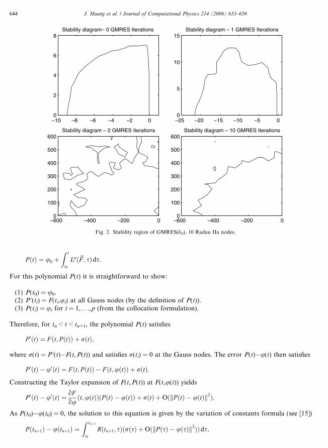
IIa nodes. For k0 = 0, this gives the original SDC, and when k0 = 4, GMRES(k0) is equivalent to the fullGMRES which solves the collocation formulation. It can be seen that the stability region of the GMRES-SDC method is much larger than that of the original SDC method. This is not surprising if one considersthe preconditioned system (31): Even though the explicit Euler method is a bad preconditioner for k with largenegative real part, the GMRES procedure can still converge to the collocation solution as long as the precon-ditioning process does not produce numerical overflow. This suggests the possibility of using explicit GMRES-SDC methods for mildly stiff problems. However, we want to mention that when more substeps are used, theexplicit Euler based preconditioner is more likely to encounter overflow problems. Hence the stability regionwill be much smaller. This can be seen in Fig. 2 where 10 Radau IIa nodes are used.
For implicit GMRES-SDC methods (using the backward Euler scheme) where the preconditioner is wellconditioned, when the full GMRES is performed, the stability regions can be considered the same as thoseof the corresponding collocation method. A-stability of these methods can be proven in some cases (all collo-cation methods using the Gaussian points are A-stable), and appears to be true for many others based onnumerical results [2]. Our numerical results also show that all the implicit GMRES-SDC methods using RadauIIa nodes we tested (up to machine precision) are A-stable. Further stability and convergence analysis for theGMRES-SDC methods are still being pursued, including the B-stability and B-convergence.
For the original SDC methods, recently, Hagstrom and Zhou showed that when p Gauss nodes are used,after 2p corrections, the order of the method is 2p [13]. This result can be generalized to the GMRES-SDCmethods which solve the collocation formulation as shown by the following theorem. Notice that whenGMRES is applied, at most p corrections are necessary for linear scalar problems, compared with 2p in [13].
Theorem 5.1. Using p Gauss nodes, the collocation method which solves Eq. (19) has order 2p.
Proof. The proof follows closely that of Theorem 1.5 in [14]. Notice that the collocation solution to Eq. (19) att is derived by spectral integration, which is equivalent to evaluating at t the degree p polynomial P(t)
Fig. 1. Stability region of GMRES(k0), 4 Radau IIa nodes.
n+1 n+1
obtained by integrating the degree p�1 interpolating polynomial Lpð~F ; sÞwhere~F ¼ ½F ðt1;u1Þ; . . . F ðtp;upÞ�T , i.e.
There
wher
Cons
As P
–10 –8 –6 –4 –2 00
2
4
6
8Stability diagram– 0 GMRES Iterations
–25 –20 –15 –10 –5 00
5
10
15Stability diagram – 1 GMRES Iterations
–600 –400 –200 00
100
200
300
400
500
600Stability diagram – 2 GMRES Iterations
–600 –400 –200 00
100
200
300
400
500
600Stability diagram – 10 GMRES Iterations
Fig. 2. Stability region of GMRES(k0), 10 Radau IIa nodes.
644 J. Huang et al. / Journal of Computational Physics 214 (2006) 633–656
Z t
P ðtÞ ¼ u0 þt0
Lpð~F ; sÞds.
For this polynomial P(t) it is straightforward to show:
(1) P(t0) = u0.(2) P 0(ti) = F(ti,ui) at all Gauss nodes (by the definition of P(t)).(3) P(ti) = ui for i = 1, . . .,p (from the collocation formulation).
fore, for tn < t < tn+1, the polynomial P(t) satisfies
P 0ðtÞ ¼ F ðt; P ðtÞÞ þ rðtÞ;
e r(t) = P 0(t)�F(t,P(t)) and satisfies r(ti) = 0 at the Gauss nodes. The error P(t)�u(t) then satisfies
P 0ðtÞ � u0ðtÞ ¼ F ðt; PðtÞÞ � F ðt;uðtÞÞ þ rðtÞ.
tructing the Taylor expansion of F(t,P(t)) at F(t,u(t)) yields
oF
P 0ðtÞ � u0ðtÞ ¼ouðt;uðtÞÞðP ðtÞ � uðtÞÞ þ rðtÞ þOðkP ðtÞ � uðtÞk2Þ.
(t0)�u(t0) = 0, the solution to this equation is given by the variation of constants formula (see [15])Z tnþ12
P ðtnþ1Þ � uðtnþ1Þ ¼t0
Rðtnþ1; sÞðrðsÞ þOðkP ðsÞ � uðsÞk ÞÞds;

where R(t,s) is the Green�s function of the corresponding homogeneous differential equation and is smoothp+1
J. Huang et al. / Journal of Computational Physics 214 (2006) 633–656 645
for s29 in
der oIIa n
Fo
beingand t
TableErrors
k0
Error
< t. Applying the theorem that the local truncation error P(t) � u(t) is at least O(Dt ) (see e.g., p.[14]), we can neglect the term O(iP(t) � u(t)i2) which is at least O(Dt2p+2) and deriveZ tnþ1
P ðtnþ1Þ � uðtnþ1Þ ¼t0
Rðtnþ1; sÞrðsÞdsþOðDt2pþ2Þ.
Since Gauss quadrature is applied to the integral and r(ti) = 0 at the Gauss nodes, the collocation solutionP(t) has the same order as the underlying quadrature formula. When Gauss–Legendre nodes are used, the or-
f the local truncation error is therefore 2p + 1. The same proof can be applied to show that when Radauodes are used, the local truncation error is O(Dt2p). h
6. Numerical experiments
In this section, we show some preliminary numerical results for both linear and nonlinear problems.Depending on the stiffness of the problem, we present results for both the explicit and implicit GMRES-SDC methods.
6.1. The cosine problem
r the first numerical example, define pðtÞ ¼ cosðtÞ and consider
u0ðtÞ ¼ p0ðtÞ � 1
eðuðtÞ � pðtÞÞ; t 2 ½0; tfinal�;
uð0Þ ¼ pð0Þ.
The exact solution is clearly u(t) = p(t). Notice that when e is small, this problem is stiff, however, the solutionitself is smooth and independent of e.
For the first example, we set e = 0.02 and Dt = 1. For each time step, we use 12 Radau IIa nodes. For thetime-stepping we use the explicit Euler method in Eq. (14). In Table 1, we show the numerical error after onestep (Dt = tfinal = 1) for different GMRES(k0). For k0 = 0, the method is the original SDC. Also, for each step,we fix the number of explicit Euler corrections to 12. The total number of function evaluations is thereforefixed to 12 · 12.
These results are consistent with the stability analysis in Section 5. Clearly, the GMRES-SDC methods givebetter numerical results even though the original SDC method is unstable. Also, for the restarted GMRES(k0),keeping more data in memory (larger k0) reduces the error. The full orthogonalization process (k0 = 12, thesame as the number of unknowns) returns converged numerical results but loses a few digits in accuracydue to the fact that the forward Euler predictor is actually unstable here (see also Fig. 3).
Next, consider the case e = 10�6. As the problem is very stiff, the implicit GMRES-SDC method is used.Note that for this example, the original SDC method is stable. As in the explicit examples, the results shownin Table 2 demonstrate that increasing k0 reduces the error and residual (defined as b�Ax when solvingAx = b) and that both go to machine precision with the full GMRES.
Note that in both the explicit and implicit examples, the error first decays slowly as a function of k0, andthen suddenly decreases to close to machine precision once k0 is the same as the number of nodes p. The con-vergence of the GMRES procedure depends in general on the distribution of the eigenvalues of the matrix
considered. In the present context, the eigenvalues of the matrix C defined in Eq. (28) are of interest,hese in turn depend on the matrix S � eS . The eigenvalues of C for both the explicit and implicit cases
1versus k0 for the cosine problem for the explicit GMRES-SDC method
0 1 2 3 4 6 12
4.2e + 57 4.6e � 1 3.8e � 3 2.1e � 3 9.2e � 4 1.7e � 4 3.6e � 13

0 0.2 0.4 0.6 0.8–0.8
–0.6
–0.4
–0.2
0
0.2
0.4
0.6
0.8
Real
Imag
Implicit Euler Method
–15 –10 –5 0 5
x 104
–0.8
–0.6
–0.4
–0.2
0
0.2
0.4
0.6
0.8
Real
Imag
Explicit Euler Method
Fig. 3. Eigenvalue distribution of C for both the implicit and explicit method. Note that the axis in the right panel are scaled by 104.
Table 2Errors and residuals versus k0 for the cosine problem for the implicit GMRES-SDC method
k0 0 1 2 3 4 6 12
Error 1.4e � 4 3.6e � 4 1.6e � 4 5.5e � 5 3.3e � 5 1.2e � 5 4.4e � 16
646 J. Huang et al. / Journal of Computational Physics 214 (2006) 633–656
above are shown in Fig. 3. The eigenvalues in the implicit case are smaller by about four orders of magnitudethan in the explicit case, but in neither case are the eigenvalues clustered about a single point.
6.1.1. Order reduction
In [24], when the original SDC method is applied to stiff problems and the number of corrections for eachstep is fixed, the effective order of accuracy is reduced for values of the time step size in a certain range. Thistype of order reduction is also present in many popular types of Runge–Kutta methods [7,8,30]. The implica-tion of order reduction is that, although the methods are stable for larger time steps, one must use a very smalltime step, or increase the number of SDC corrections for the method to converge with full order. However,with the GMRES-SDC methods, when full orthogonalization is used, order reduction is no longer observed.In Fig. 4, convergence results are presented for both the original SDC and the new implicit GMRES-SDCmethods for different e and step size selections. In the calculation, 10 Radau IIa nodes are used, and 10 iter-ations are performed. The order reduction phenomenon can be easily observed when e is small (curves on the
Residual 2.3e � 4 2.9e � 4 1.6e � 4 8.1e � 5 4.8e � 5 1.6e � 5 2.8e � 16
left). The plots also indicate the benefit in terms of computational cost the GMRES acceleration provides. Forexample, when e = 10�5, in order to have 13 digits of accuracy, the original SDC requires a step size of

10–4
10–3
10–2
10–1
100
101
10–14
10–12
10–10
10–8
10–6
10–4
10–2
100
step size
erro
r
Comparison of original SDC (O) with GMRES accelerated SDC (G)
ε=10–1, O
ε=10–2, O
ε=10–3, O
ε=10–4, O
ε=10–5, O
ε=10–1, G
ε=10–2, G
ε=10–3, G
ε=10–4, G
ε=10–5, G
J. Huang et al. / Journal of Computational Physics 214 (2006) 633–656 647
approximately 10�5. For the GMRES-SDC method with full orthogonalization, the necessary step size isapproximately 0.1, or 4 orders of magnitude greater.
6.2. The linear multiple mode problem
As mentioned above, the convergence of a GMRES-SDC method will depend on the eigenvalues of thematrix C in Eq. (28), which depend also on the eigenvalues of the linear operator L. Hence in our secondset of tests, we study an ODE system similar to the cosine problem in which we can specify the distributionof the eigenvalues. When GMRES is applied to the original SDC, it is usually expensive to use the full orthog-onalization process since it would require k0 = pN iterations for a system of N ODEs using p nodes. Thisincreases both the memory required and the amount of work performed. Therefore a natural question is, givensome information on the distribution of the eigenvalues, can we determine the ‘‘optimal’’ number k0? The fol-
Fig. 4. Order reduction: the original SDC and the GMRES-SDC.
lowing numerical experiments are intended to provide some basic guidelines.Th
wherestruct
tion.to 1. I
e problem studied in this example is
�y0ðtÞ ¼ �p0ðtÞ � Bð�yðtÞ � �pðtÞÞ;
�yð0Þ ¼ �pð0Þ;�yðtÞ and �pðtÞ are vectors of dimension N. The exact solution is again �yðtÞ ¼ �pðtÞ. The matrix B is con-
ed byB ¼ U TKU ;
where U is a randomly generated orthogonal matrix, and K is a diagonal matrix whose diagonal entries fkigNi¼1
are all positive. For �pðtÞ, we choose the ith component as cosðt þ aiÞ with phase parameter ai = 2pi/N.In our first experiment, we set the dimension of the system to 10, and use 10 Radau IIa nodes in the simula-
7
We use Dt = 0.1 and study one time step (i.e., tfinal = Dt). In the left of Fig. 5, we set k1 = 10 , and all other kit can be seen that when k0 � 12, the residual converges to machine precision in about 25 iterations. Notice

0 10 20 30 4010
–16
10–14
10–12
10–10
10–8
10–6
10–4
10–2
100
Number of corrections
Res
idua
l1 eigenvalue cluster point
k0=1k0=5k0=10k0=12
0 10 20 30 40
10–14
10–12
10–10
10–8
10–6
10–4
10–2
100
Number of corrections
Res
idua
l
2 eigenvalue cluster points
k0=1k0=5k0=10k0=15k0=20k0=25
648 J. Huang et al. / Journal of Computational Physics 214 (2006) 633–656
that 10 Radau IIa nodes resolve the solution to 14 digits, therefore the residual is equivalent to the error (up to aconstant factor). In the right panel, results are shown for the case when two eigenvalues are 107, two are 104, andthe rest are 1. In this case, more iterations are required to reduce the residual to machine precision, and itrequires a slightly higher k0 of approximately 15 to yield the best convergence results (i.e. results for k0 = 15are almost identical to those using larger k0). However, these values of k0 are much smaller compared withthe full GMRES which requires k0 = 100. Since the original SDC method would require ten iterations of thecorrection equation, in this case, there is a factor of 4 increase in the number of iterations for GMRES-SDCmethod, however, this results in a reduction in the error of approximately 10 orders of magnitude.
In our second experiment, we consider the case where N = 100 and the log10 of the eigenvalues are uni-formly distributed on [0,7]. For 10 Radau IIa nodes, numerical results for different k0 are shown in Fig. 6.In this example, convergence profiles for k0 > 10 are very similar. Notice that the full GMRES requiresk0 = 1000, hence only a small fraction of the full method is required for machine precision. At present, theoptimal strategy for picking k0 for a given problem is not completely understood, although these experimentssuggest that a successful strategy must depend on the time step, the size of the system, the distribution of theeigenvalues, and of course any memory restrictions based on the problem size. The authors are currently inves-tigating strategies for choosing k0 in the broader context of step size selection.
6.3. The Van der Pol oscillator
In our third example, we consider the nonlinear ODE initial value problem which describes the behavior of
Fig. 5. Comparison of errors for different k0.
vacuum tube circuits. It was proposed by B. Van der Pol in the 1920�s, and is often referred to as the Van derPol oscillator. As a first order ODE system, the problem takes the form

resultconve
0 5 10 15 20 25 30 35 40 45 5010
–14
10–12
10–10
10–8
10–6
10–4
10–2
100
Number of corrections
Res
idua
l
log10
(Eigenvalues) uniformly distributed in [0, 7], convergence for different k0
k0=1k0=5k0=10k0=15k0=20k0=50
Fig. 6. Comparison of errors for different k .
J. Huang et al. / Journal of Computational Physics 214 (2006) 633–656 649
y 0 ðtÞ ¼ y2ðtÞ;�
0
1
0 2ð40Þ
y2ðtÞ ¼ ð1� y1ðtÞy2ðtÞ � y1ðtÞÞ=e;
where the initial values are given by [y(0),y 0(0)] = [2,�0.6666654321121172]. This is a stiff system when e issmall. For this nonlinear problem, we use the ‘‘linear implicit’’ GMRES-SDC methods discussed in Section4, and choose the following strategy in the implementation: GMRES(k0) is applied to the linearized systemuntil the residual b�Ax is reduced by a factor of tolG; once this is done, we update the Jacobian matrixand restart GMRES(k0).
As our first experiment, we set e = 10�3, and use Dt = 0.001. We apply the explicit GMRES-SDC method,and in Fig. 7, we show how the residual decays (as the analytical solution is not readily available) for differentk0 when tolG = 0.01 (left) and tolG = 0.1 (right). Here, the residual is defined as the error ib�Axi for the lin-earized system in Eq. (36). It can be seen that the GMRES-SDC method converges quickly to the solution ofthe collocation formulation. This is consistent with the stability analysis in Section 5 and the linear cosine testproblems in Section 6.1. Notice that for this problem, the original SDC method is divergent (not shown onplot), and GMRES(1) converges very slowly.
Because of the nonlinearity of the problem, the convergence behavior of the GMRES-SDC method alsodepends on tolG. The two panels in Fig. 7 compare convergence for tolG = 0.01 and tolG = 0.1. In the leftpanel, it appears that using k0 = 10 is sufficient for achieving the best convergence results since the conver-gence for k0 = 15 is nearly identical. In the right panel, convergence for k0 = 5 is the same as for k0 = 10and k0 = 15, although the overall number of iterations required to achieve a specified error tolerance increasesslightly compared to tolG = 0.01. Determining the ‘‘optimal’’ choice of tolG or an adaptive strategy for choos-ing tolG is an open issue.
Next we apply the implicit GMRES-SDC method to the very stiff case with e = 10�8 and Dt = 0.5. The
s are shown in Fig. 8 for different choices of k0 and tolG = 0.1. In all cases, the GMRES-SDC methodsrge more rapidly to the collocation solution than the original SDC method.
0 10 20 30 4010
–14
10–12
10–10
10–8
10–6
10–4
10–2
Number of corrections
Res
idua
ltol
G=0.01
0 10 20 30 4010
–14
10–12
10–10
10–8
10–6
10–4
10–2
Number of corrections
Res
idua
l
tolG
=0.1
k0=1k0=2k0=5k0=10k0=15
k0=1k0=2k0=5k0=10k0=15
Fig. 7. Comparison of different k0 for the Van der Pol problem, explicit method.
650 J. Huang et al. / Journal of Computational Physics 214 (2006) 633–656
It is possible to apply a different numerical method for the time marching of the correction equation. In theabove examples, either the explicit or implicit Euler method is used for the correction equation. It is reasonableto expect that the use of a higher-order numerical method for the time marching of the correction equationwould result in a method which requires fewer iterations of the correction equation to converge to a specifiedtolerance. In the linear case, this is equivalent to choosing a different preconditioner for the Neumann seriesexpansion. We investigate this idea by repeating the above numerical example using the trapezoid rule. Theresults are compared with those from the implicit Euler method in Fig. 9 for k0 = 1, 2 and 10. From this figure,we can see that using larger k0 again improves the numerical convergence in both cases. However, whenk0 = 10, the trapezoid rule results are not significantly better than those computed with the first-order method.Hence, at least for this limited experiment, using a higher-order marching method does not seem to have asignificant effect on the convergence when the GMRES acceleration procedure is used (see also [19]).
6.4. The nonlinear multi-mode problem
Inis giv
The awith
this example, we study a nonlinear generalization of the multi-mode example in Section 6.2. The problemen by a system of N nonlinear equations
y0ðtÞ ¼ p0ðtÞ � kiyiþ1ðtÞðyiðtÞ � piðtÞÞ; 1 < i < N � 1;�
i i
y0N ðtÞ ¼ p0N ðtÞ � kiðyiðtÞ � piðtÞÞ; i ¼ N .
nalytical solution is again �yðtÞ ¼ �pðtÞ where the ith component of �pðtÞ is given by piðtÞ ¼ 2þ cosðt þ aiÞphase parameter ai = 2pi/N. In our first experiment, we set N = 7 and the eigenvalues are chosen as

0 10 20 30 40 50 60
10–14
10–12
10–10
10–8
10–6
10–4
10–2
Number of corrections
Res
idua
l
tolG
=0.1, implicit method
k0=1
k0=2
k0=5
k0=10
k0=15
Fig. 8. Comparison of different k0 for the very stiff Van der Pol problem with implicit method.
0 5 10 15 20 25 30 35 40
10–14
10–12
10–10
10–8
10–6
10–4
Number of corrections
Res
idua
l
Comparsion of trapezoidal rule (t) with implicit Euler (e) for different k0
k0=1,ek0=2,ek0=10,ek0=1,tk0=2,tk0=10,t
Fig. 9. Comparison using trapezoidal rule versus the implicit Euler method.
J. Huang et al. / Journal of Computational Physics 214 (2006) 633–656 651
20 40 6010
–14
10–12
10–10
10–8
10–6
10–4
10–2
100
102
Number of corrections
Res
idua
l1 eigenvalue cluster point
k0=1
k0=2
k0=5
k0=10
k0=15
20 40 60 8010
–14
10–12
10–10
10–8
10–6
10–4
10–2
100
102
Number of corrections
Res
idua
l
2 eigenvalue cluster points
k0=1
k0=2
k0=5
k0=10
k0=15
Fig. 10. Nonlinear multi-mode convergence.
652 J. Huang et al. / Journal of Computational Physics 214 (2006) 633–656
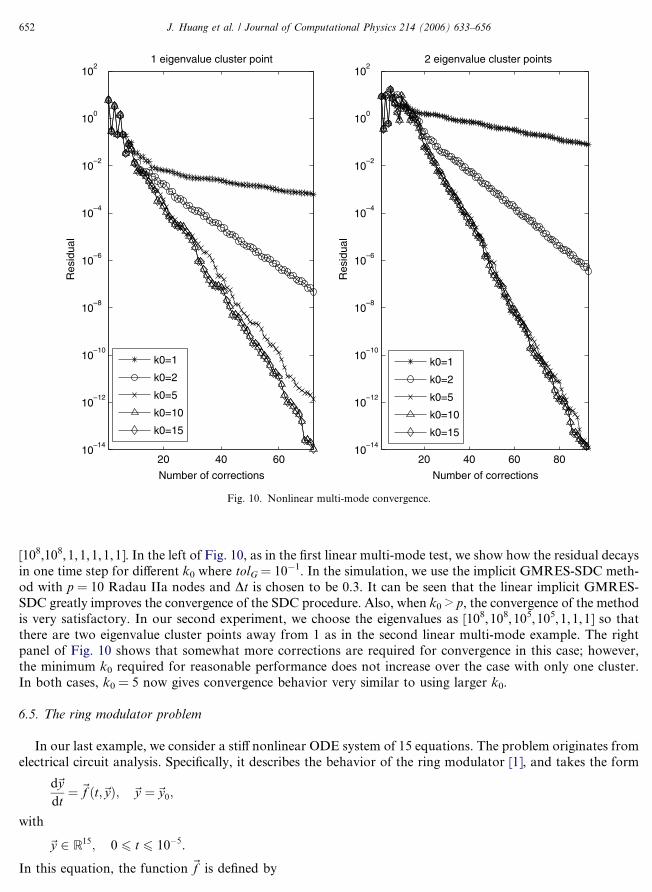
[108,108,1,1,1,1,1]. In the left of Fig. 10, as in the first linear multi-mode test, we show how the residual decaysin one time step for different k0 where tolG = 10�1. In the simulation, we use the implicit GMRES-SDC meth-od with p = 10 Radau IIa nodes and Dt is chosen to be 0.3. It can be seen that the linear implicit GMRES-SDC greatly improves the convergence of the SDC procedure. Also, when k0 > p, the convergence of the methodis very satisfactory. In our second experiment, we choose the eigenvalues as [108,108,105,105,1,1,1] so thatthere are two eigenvalue cluster points away from 1 as in the second linear multi-mode example. The rightpanel of Fig. 10 shows that somewhat more corrections are required for convergence in this case; however,the minimum k0 required for reasonable performance does not increase over the case with only one cluster.In both cases, k0 = 5 now gives convergence behavior very similar to using larger k0.
6.5. The ring modulator problem
Inelectr
with
In th
our last example, we consider a stiff nonlinear ODE system of 15 equations. The problem originates fromical circuit analysis. Specifically, it describes the behavior of the ring modulator [1], and takes the form
d~ydt¼ ~f ðt;~yÞ; ~y ¼~y0;
~y 2 R15; 0 6 t 6 10�5.
is equation, the function ~f is defined by

The a
and t
Ousolve
~f ðt;~yÞ ¼
C�1ðy8 � 0:5y10 þ 0:5y11 þ y14 � R�1y1ÞC�1ðy9 � 0:5y12 þ 0:5y13 þ y15 � R�1y2Þ
C�1s ðy10 � qðU D1Þ þ qðU D4ÞÞ
�C�1s ðy11 � qðUD2Þ þ qðU D3ÞÞ
C�1s ðy12 þ qðU D1Þ � qðU D3ÞÞ
�C�1s ðy13 þ qðUD2Þ � qðU D4ÞÞ
C�1p ð�R�1
p y7 þ qðU D1Þ þ qðU D2Þ � qðUD3Þ � qðU D4ÞÞ�L�1
h y1
�L�1h y2
L�1s2 ð0:5y1 � y3 � Rg2y10Þ�L�1
s3 ð0:5y1 � y4 þ Rg3y11ÞL�1
s2 ð0:5y2 � y5 � Rg2y12Þ�L�1
s3 ð0:5y2 � y6 þ Rg3y13ÞL�1ð�y þ U in1ðtÞ � ðRi þ Rg4Þy Þ
0BBBBBBBBBBBBBBBBBBBBBBBBBBBBBBB@
1CCCCCCCCCCCCCCCCCCCCCCCCCCCCCCCA
.
J. Huang et al. / Journal of Computational Physics 214 (2006) 633–656 653
s1 1 14
L�1s1 ð�y2 � ðRc þ Rg1Þy15Þ
uxiliary functions UD1,UD2,UD3,UD4,q,Uin1 and Uin2 are given by
U D1 ¼ y3 � y5 � y7 � U in2ðtÞ;U D2 ¼ �y4 þ y6 � y7 � U in2ðtÞ;U D3 ¼ y4 þ y5 � y7 þ U in2ðtÞ;U D4 ¼ �y3 � y6 þ y7 þ U in2ðtÞ;qðUÞ ¼ cðedU � 1Þ;U in1ðtÞ ¼ 0:5 sinð2000ptÞ;
U in2ðtÞ ¼ 2 sinð2000ptÞ.eters are
The values of the paramr results suggest that the new GMRES-SDC method is a very competitive alternative trs. However, in order to perform more extensive (and convincing) tests, an automatic ste
C = 1.6 Æ 10�8
R = 25000 C = 2 · 10�12 R = 50 sC = 10�8
iR = 50
p pLh = 4.45
Lc = 600 Ls1 = 0.002�4
Rg1 = 36.3Ls2 = 5 · 10�4
Rg2 = 17.3
Ls3 = 5 · 10 Rg3 = 17.3c = 40.67286402 · 10�9 d = 17.7493332he initial value ~y0 is given by
~y0 ¼~0.
In the simulation, we use the implicit GMRES-SDC method with p = 7 Radau IIa nodes. We set tolG = 0.1,k0 = p + 1, and tfinal = 10�5. Our uniform step GMRES-SDC method is then compared with available adaptive
ODE packages described in [1] and the results are shown in Table 3. In the table, the parameters rtol, atol andh0 for each method are chosen experimentally to produce a numerical solution with at least 9 significant digits,which has the fewest possible number of function evaluations.
o existing ODEp-size selection

Table 3Performance comparison of different solvers
G-SDC DASSL GAMD MEBDFI PSIDE RADAU VODE
Rtol 1e � 8 1e � 12 1e � 10 1e � 9 1e � 10 1e � 9 1e � 11Atol * 1e � 12 1e � 10 1e � 11 1e � 11 1e � 10 1e � 14h0 2.5e � 6 * 1e � 10 1e � 10 * 1e � 10 *
Rerr 3.0e � 9 1.1e � 9 3.1e � 9 2.9e � 9 2.1e � 9 2.1e � 9 1.3e � 9F 1134 2104 4057 2284 3417 2172 2961Steps 4 1591 76 669 154 47 2277
*, not needed; rtol, relative tolerance; atol, absolute tolerance; h0, initial step-size; rerr, maximum relative error; F, number of functionevaluations; steps, number of steps taken.
0 0.2 0.4 0.6 0.8 1
x 10–5
10–9
10–8
10–7
10–6
time
step
size
RADAUMEBDFI
654 J. Huang et al. / Journal of Computational Physics 214 (2006) 633–656
strategy is required for the GMRES-SDC method. In Fig. 11, we show the step-sizes used by the adaptive solv-ers MEBDFI and RADAU. Currently, we are studying strategies for step-size selections along with strategiesfor computing better initial provisional solutions, for adaptively choosing the parameters k0 and tolG, and foradaptively varying the order of the SDC method. Progress will be reported in the future.
Finally for this section, we want to mention that we have also studied several other problems from the TestSet for IVP solvers [1]. In all cases, the convergence of the original SDC methods is greatly improved by theGMRES-SDC procedure.
7. Conclusions
In this paper, a matrix based analysis of the original SDC method for linear problems shows that the iter-ated corrections are equivalent to a preconditioned Neumann series expansion. By introducing the Krylovsubspace based GMRES method, we show how the convergence of the original SDC can be accelerated. Pre-liminary analytical and numerical results show that the stability and accuracy of this new class of methods aregreatly improved for both linear and nonlinear problems compared to the original method.
In order to fully explore the efficiency of the new accelerated SDC methods, a direct comparison with exist-
Fig. 11. Step-sizes selected by RADAU and MEBDFI.
ing methods on standard test problems needs to be carried out. This requires that a variable time step selectionalgorithm be implemented with the GMRES-SDC method. The authors have been investigating strategies for

varying both the time step and the order of the method to optimally achieve a desired error tolerance. Theproblem of developing a robust algorithm is further complicated by the fact that the performance of theGMRES acceleration depends on the size of the time step, the size of the system, the stiffness of the equation,and on the restart parameter k0. We have also investigated more effective methods of coupling the GMRESprocess with Newton�s method for the implicit version on nonlinear problems. Results along these lines will bepresented in the future.
One case where it is clear that the GMRES acceleration is advantageous is for ODE initial value problemswhere the stiffness is caused by only a few eigenvalues with large negative real parts. For this case, the reduc-tion to first order accuracy for a range of time step size which is observed for the original SDC methods iseffectively eliminated in the tests presented in Section 6.1. The analysis here clearly shows that order reductionis equivalent to the slow decay of the Neumann series expansion derived in Section 3.
Several other extensions of the accelerated method are also being pursued. One advantageous feature ofSDC methods in general is that semi- and multi-implicit versions of the method for problems with more thanone stiff time scale have been developed [6,26]. Acceleration of these methods is also being pursued. It shouldbe noted that for PDE applications (for which the semi- and multi-implicit methods were developed), the sizeof the linear system that GMRES is being applied to in the current methods may be very large, and hencememory restrictions may require that a small restart parameter k0 be used. More numerical tests need tobe conducted in such cases to determine the benefits of the GMRES acceleration.
J. Huang et al. / Journal of Computational Physics 214 (2006) 633–656 655
Finally, a generalization of the GMRES-SDC method has been applied to differential algebraic equations.
Initial numerical results are very promising, and a paper reporting on these results is in preparation [21].Acknowledgements
The work of J.H. and J.J. was supported in part by the NSF under Grants DMS0411920 and DMS0327896.M.M. was supported in part under Contract De-AC03-76SF00098 by the Director, Department of Energy(DOE) Office of Science; Office of Advanced Scientific Computing Research; Office of Mathematics, Informa-tion, and Computational Sciences.
References
[1] http://pitagora.dm.uniba.it/~testset/.[2] R. Barrio, On the A-stability of Runge–Kutta collocation methods based on orthogonal polynomials, SIAM J. Numer. Anal. 36 (4)
(1999) 1291–1303.[3] K.E. Brenan, S.L. Campbell, L.R. Petzold, Numerical Solution of Initial-Value Problems in Differential-Algebraic Equations, SIAM,
Philadelphia, 1995.[4] J. Butcher, The Numerical Analysis of Ordinary Differential Equations: Runge–Kutta and General Linear Methods, Wiley, 1987.[5] K. Bohmer, H.J. Stetter (Eds.), Defect Correction Methods, Theory and Applications, Springer-Verlag, Wien-New York, 1984.[6] A. Bourlioux, A.T. Layton, M.L. Minion, High-order multi-implicit spectral deferred correction methods for problems of reactive
flow, J. Comput. Phys. 189 (2003) 351–376.[7] M.P. Calvo, C. Palencia, Avoiding the order reduction of Runge–Kutta methods for linear initial boundary value problems, Math.
Comput. 71 (2002) 1529–1543.[8] K. Dekker, J.G. Verwer, in: Stability of Runge–Kutta Methods for Stiff Nonlinear Differential EquationsCWI Monographs, North-
Holland, 1984.[9] A. Dutt, L. Greengard, V. Rokhlin, Spectral deferred correction methods for ordinary differential equations, BIT 40 (2) (2000) 241–
266.[10] C.W. Gear, Numerical Initial Value Problems in Ordinary Differential Equations, Prentice-Hall, New Jersey, 1971.[11] D. Gottlieb, S.A. Orszag, Numerical Analysis of Spectral Methods, SIAM, Philadelphia, 1977.[12] L. Greengard, Spectral integration and two-point boundary value problems, SIAM J. Numer. Anal. 28 (1991) 1071–1080.[13] T. Hagstrom, R. Zhou, On the spectral deferred correction of splitting methods for initial value problems, CAMCos (submitted).[14] E. Hairer, C. Lubich, G. Wanner, Geometric Numerical Integration: Structur-Preserving Algorithms for Ordinary Differential
Equaitons, Springer-Verlag, Berlin, 2002.[15] E. Hairer, S.P. Norsett, G. Wanner, Solving Ordinary Differential Equations I, Non-Stiff Problems, Springer-Verlag, Berlin, 1993.[16] E. Hairer, G. Wanner, Solving Ordinary Differential Equations II, Springer-Verlag, Berlin, 1996.[17] E. Hairer, C. Lubich, M. Roche, The Numerical Solution of Differential-Algebraic Systems by Runge–Kutta Methods, Springer-
Verlag, Berlin, 1989.[18] A.C. Hansen, J. Strain, On the order of deferred correction, BIT (submitted).

[19] A.C. Hansen, J. Strain, Convergence theory for spectral deferred correction, (in press).[20] D.J. Higham, L.N. Trefethen, Stiffness of ODEs BIT 33 (1993) 285–303.[21] J. Huang, J. Jia, M.L. Minion, Arbitrary order Krylov deferred correction methods for differential algebraic equations, Prog. Appl.
Math. Preprint Series, University of North Carolina, PAMPS 2005-01.[22] C.T. Kelly, Solving Nonlinear Equations with Newton�s Method, SIAM, 2003.[23] J.D. Lambert, Numerical Methods for Ordinary Differential Equations, Wiley, Berlin, 1991.[24] A.T. Layton, M.L. Minion, Implications of the choice of quadrature nodes for Picard integral deferred corrections methods for
ordinary differential equations, BIT 45 (2005) 341–373.[25] B. Lindberg, Error estimation and iterative improvement for discretization algorithms, BIT 20 (1980) 486–500.[26] M.L. Minion, Semi-implicit spectral deferred correction methods for ordinary differential equations, CMS 1 (2003) 471–500.[27] M.L. Minion, Semi-implicit projection methods for incompressible flow based on spectral deferred corrections, APNUM 48 (3–4)
(2004) 369–387.[28] V. Pereyra, Iterated deferred correction for nonlinear boundary value problems, Numer. Math. 11 (1968) 111–125.[29] Y. Saad, M.H. Schultz, GMRES: a generalized minimal residual algorithm for solving non-symmetric linear systems, SIAM J. Sci.
Stat. Comp. 7 (1986) 856–869.[30] J.M. Sanz-Serna, J.G. Verwer, W.H. Hundsdorfer, Convergence and order reduction of Runge–Kutta schemes applied to
evolutionary problems in partial differential equations, Numer. Math. 50 (1986) 405–418.[31] R.D. Skeel, A theoretical framework for proving accuracy results for deferred correction, SIAM J. Numer. Anal. 19 (1981) 171–196.[32] J. Stoer, R. Bulirsch, Introduction to Numerical Analysis, Springer, Berlin, 1992.[33] L.N. Trefethen, M.R. Trummer, An instability phenomenon in spectral methods, SIAM J. Numer. Anal. 24 (1987) 9.[34] P.E. Zadunaisky, A method for the estimation of errors propagated in the numerical solution of a system of ordinary differential
equations, The theory of orbits in the solar system and in stellar systems, in: Proceedings of International Astronomical Union,Symposium, vol. 25, 1964.
[35] P.E. Zadunaisky, On the estimation of errors propagated in the numerical integration of ordinary differential equations, Numer.
656 J. Huang et al. / Journal of Computational Physics 214 (2006) 633–656
Math. 27 (1976) 21–40.


