

OPRE 6364 1
Acceptance Sampling

OPRE 6364 2
Acceptance Sampling
● Accept/reject entire lot based on sample results● Created by Dodge and Romig during WWII● Not consistent with TQM of Zero Defects● Does not estimate the quality of the lot

OPRE 6364 3
What is acceptance sampling?
Lot Acceptance Sampling– A SQC technique, where a random sample is
taken from a lot, and upon the results of appraising the sample, the lot will either be rejected or accepted
– A procedure for sentencing incoming batches or lots of items without doing 100% inspection
– The most widely used sampling plans are given by Military Standard (MIL-STD-105E)

OPRE 6364 4
What is acceptance sampling?
• Purposes– Determine the quality level of an incoming
shipment or at the end of production– Judge whether quality level is within the level
that has been predetermined
• But! Acceptance sampling gives you no idea about the process that is producing those items!
OPRE 6364 5
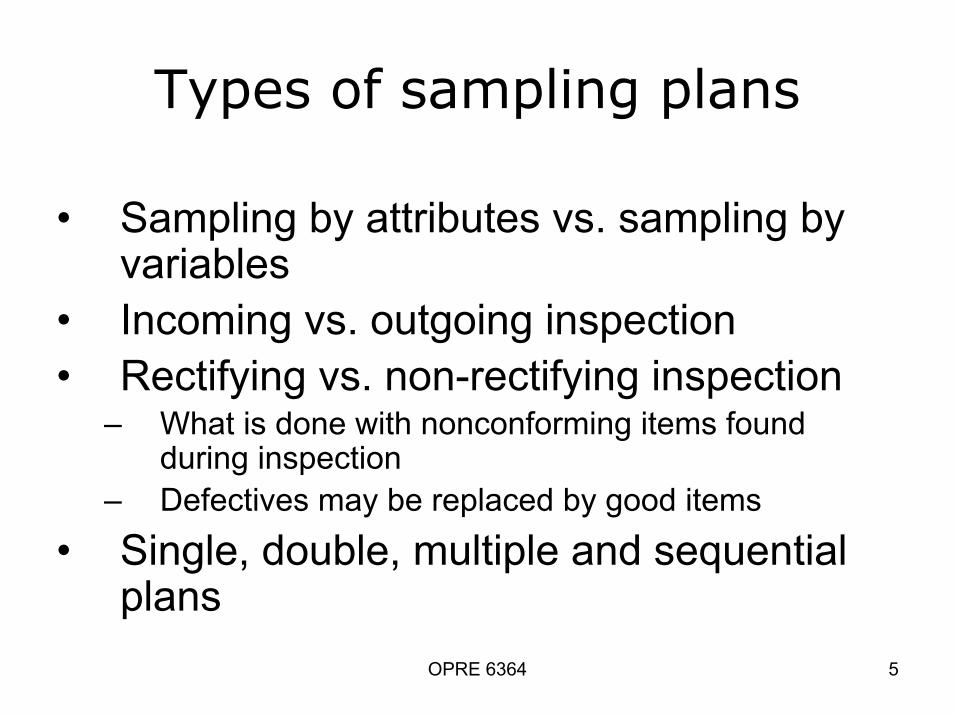
Types of sampling plans
• Sampling by attributes vs. sampling by variables
• Incoming vs. outgoing inspection• Rectifying vs. non-rectifying inspection
– What is done with nonconforming items found during inspection
– Defectives may be replaced by good items• Single, double, multiple and sequential
plans

OPRE 6364 6
How acceptance sampling works
• Attributes(“go no-go” inspection)– Defectives-product acceptability across range– Defects-number of defects per unit
• Variable (continuous measurement)– Usually measured by mean and standard
deviation

OPRE 6364 7
Why use acceptance sampling?
• Can do either 100% inspection, or inspect a sample of a few items taken from the lot
• Complete inspection– Inspecting each item produced to see if each
item meets the level desired– Used when defective items would be very
detrimental in some way

OPRE 6364 8
Why not 100% inspection?
Problems with 100% inspection– Very expensive– Can’t use when product must be destroyed to
test– Handling by inspectors can induce defects– Inspection must be very tedious so defective
items do not slip through inspection

OPRE 6364 9
A Lot-by-Lot Sampling Plan
N(Lot) n
Count Number
Conforming
Accept orReject Lot
• Specify the plan (n, c) given N • For a lot size N, determine
– the sample size n, and – the acceptance number c.
• Reject lot if number of defects > c • Specify course of action if lot is rejected

OPRE 6364 10
The Single Sampling Plan
• The most common and easiest plan to use but not most efficient in terms of average number of samples needed
• Single sampling planN = lot sizen = sample size (randomized)c = acceptance numberd = number of defective items in sample
• Rule: If d ≤ c, accept lot; else reject the lot

OPRE 6364 11
d ≤ c ?
Reject lot
YesAccept lot
Do 100% inspection
Return lot to supplier
Inspect all items in the sample
Defectives found = d
No
Take a randomized sample of size n
from the lot NThe Single Sampling procedure

OPRE 6364 12
Producer’s & Consumer’s Risksdue to mistaken sentencing
• TYPE I ERROR = P(reject good lot)α or Producer’s risk 5% is common
• TYPE II ERROR = P(accept bad lot)β or Consumer’s risk10% is typical value

OPRE 6364 13
Quality Definitions• Acceptance quality level (AQL)
The smallest percentage of defectives that will make the lot definitely acceptable. A quality level that is the base line requirement of the customer
• RQL or Lot tolerance percent defective (LTPD)Quality level that is unacceptable to the customer

OPRE 6364 14
How acceptance sampling works
• Remember– You are not measuring the quality of the
lot, but, you are to sentence the lot to either reject or accept it
• Sampling involves risks:– Good product may be rejected– Bad product may be accepted
Because we inspect only a sample, not the whole lot!

OPRE 6364 15
Acceptance sampling contd.
• Producer’s risk– Risk associated with a lot of acceptable quality
rejected
• Alpha α= Prob (committing Type I error) = P (rejecting lot at AQL quality level) = producers risk
OPRE 6364 16
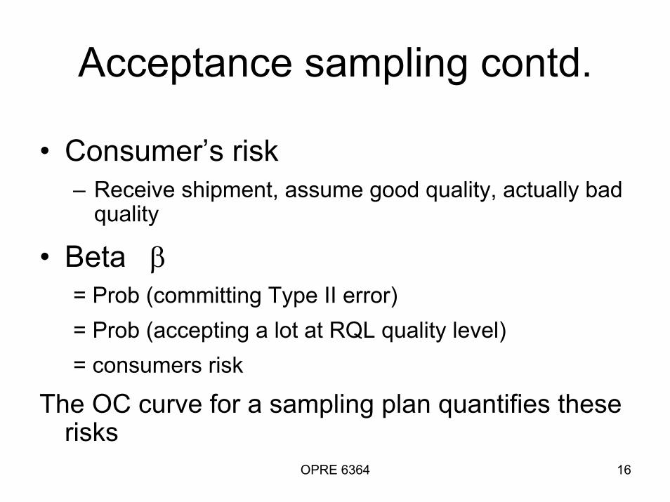
Acceptance sampling contd.
• Consumer’s risk– Receive shipment, assume good quality, actually bad
quality
• Beta β= Prob (committing Type II error)= Prob (accepting a lot at RQL quality level) = consumers risk
The OC curve for a sampling plan quantifies these risks

OPRE 6364 17
Take a randomized sample of size n from
the lot of unknown quality p
The Single Sampling procedureInspect all items in the
sampleDefectives found = d
d ≤ c ?
No
Yes
Reject lot
Accept lot
Return lot to supplier
Do 100% inspection
OPRE 6364 18
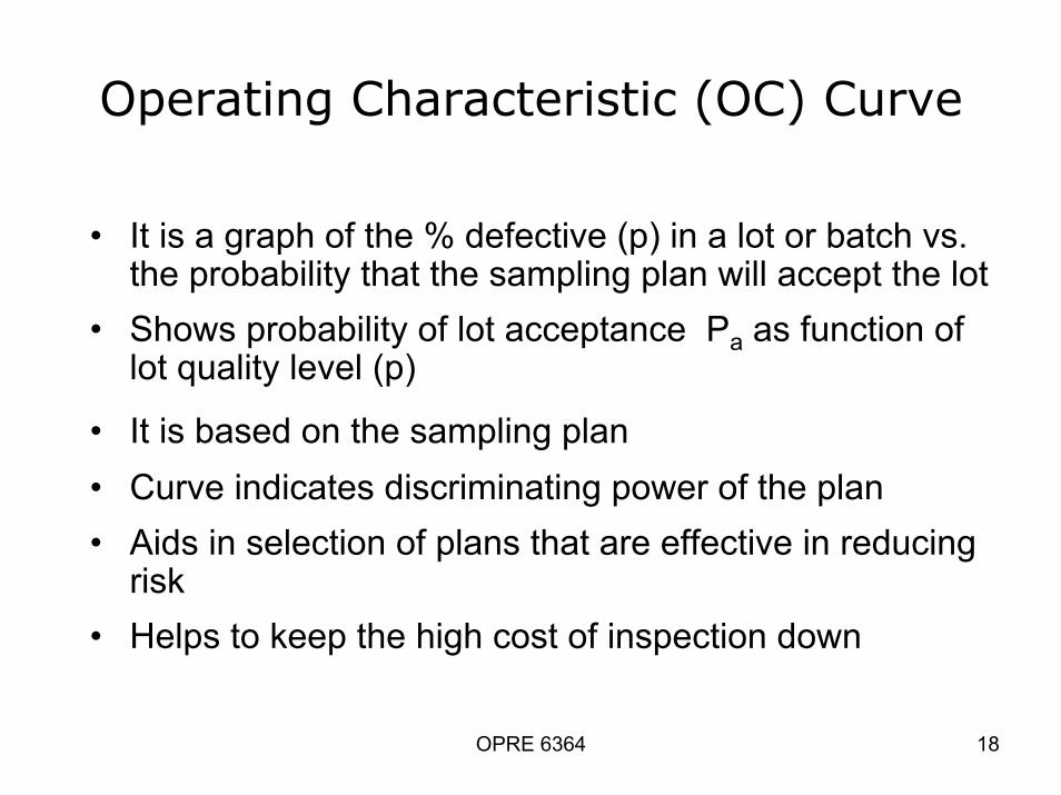
Operating Characteristic (OC) Curve
• It is a graph of the % defective (p) in a lot or batch vs. the probability that the sampling plan will accept the lot
• Shows probability of lot acceptance Pa as function of lot quality level (p)
• It is based on the sampling plan• Curve indicates discriminating power of the plan• Aids in selection of plans that are effective in reducing
risk • Helps to keep the high cost of inspection down

OPRE 6364 19
Operating Characteristic Curve
AQL LTPD
β = 0.10
α = 0.05Pr
obab
ility
of
acce
pta
nce
, P a
{
0.60
0.40
0.20
0.02 0.04 0.06 0.08 0.10 0.12 0.14 0.16 0.18 0.20
0.80
{
Proportion defective p
1.00
OC curve for n and c

OPRE 6364 20
Types of OC Curves
• Type A– Gives the probability of acceptance for an individual
lot coming from finite production• Type B
– Give the probability of acceptance for lots coming from a continuous process or infinite size lot

OPRE 6364 21
OC Curve Calculation
The Ways of Calculating OC Curves– Binomial distribution– Hypergeometric distribution
• Pa = P(r defectives found in a sample of n)– Poisson formula
• P(r) = ( (np)r e-np)/ r!– Larson nomogram

OPRE 6364 22
OC Curve Calculation by Poisson distribution
• A Poisson formula can be used– P(r) = ((np)r e-np) /r! = Prob(exactly r defectives in n)
• Poisson is a limit – Limitations of using Poisson
• n ≤ N/10 total batch • Little faith in Poisson probability calculation when n
is quite small and p quite large.• For Poisson, Pa = P(r ≤ c)

OPRE 6364 23p
For us, Pa = P(r ≤ c)
OPRE 6364 24
OC Curve Calculation by Binomial Distribution
Note that we cannot always use the binomial distribution because
• Binomials are based on constant probabilities– N is not infinite– p changes as items are drawn from the lot

OPRE 6364 25
OC Curve by Binomial Formula
.12 .115
.11 .162
.10 .223
.09 .300
.08 .394
.07 .502
.06 .620
.05 .739
.04 .845
.03 .930
.02 .980
.01 .998 PdPa
Using this formula with n = 52 and c=3 and p = .01, .02, ...,.12 we find data values as shown on the right. This givens the plot shown below.

OPRE 6364 26
The Ideal OC Curve
● Ideal curve would be perfectly perpendicular from 0 to 100% for a fraction defective = AQL
● It will accept every lot with p ≤ AQL and reject every lot with p > AQL
p AQL
1.0
0.0
Pa
OPRE 6364 27
Properties of OC Curves
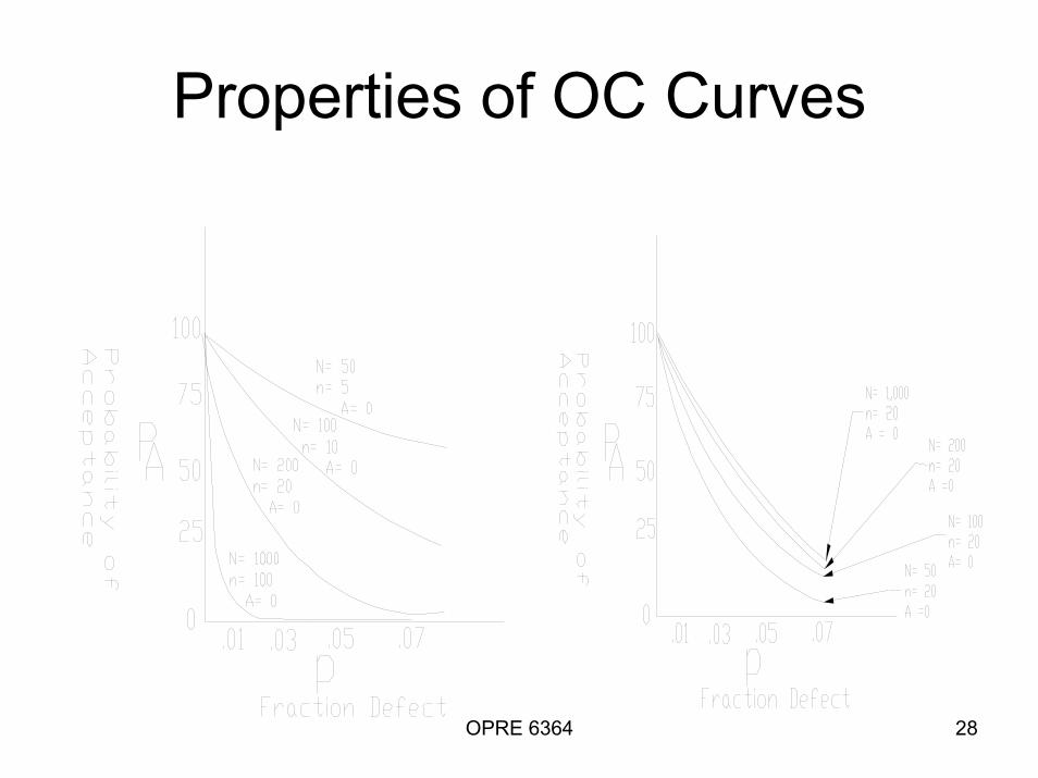
• The acceptance number c and sample size n are most important factors in defining the OC curve
• Decreasing the acceptance number is preferred over increasing sample size
• The larger the sample size the steeper is the OC curve (i.e., it becomes more discriminating between good and bad lots)
OPRE 6364 28
Properties of OC Curves

OPRE 6364 29
Properties of OC Curves
• If the acceptance level c is changed, the shape of the curve will change. All curves permit the same fraction of sample to be nonconforming.
OPRE 6364 30
Average Outgoing Quality (AOQ)
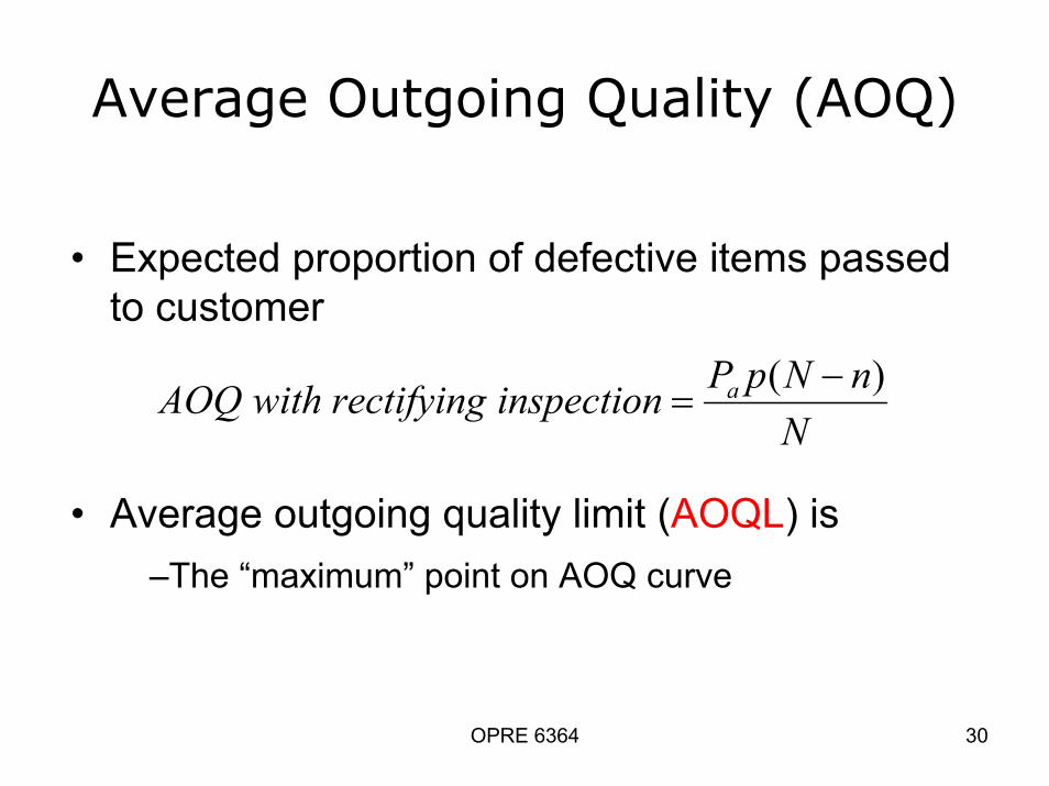
• Expected proportion of defective items passed to customer
• Average outgoing quality limit (AOQL) is–The “maximum” point on AOQ curve
NnNpPinspectionrectifyingwithAOQ a )( −
=

OPRE 6364 31
AOQ Curve
0.015AOQL
AverageOutgoingQuality
0.010
0.005
0.100.090.01 0.02 0.03 0.04 0.05 0.06 0.07 0.08
AQL LTPD
(Incoming) Percent Defective
OPRE 6364 32
Double Sampling Plans
• Take small initial sample–If # defectives < lower limit, accept–If # defectives > upper limit, reject–If # defectives between limits, take second sample
• Accept or reject lot based on 2 samples• Less inspection than in single-sampling

OPRE 6364 33
Multiple Sampling Plans
• Advantage: Uses smaller sample sizes• Take initial sample
–If # defectives < lower limit, accept–If # defectives > upper limit, reject–If # defectives between limits, re-sample
• Continue sampling until accept or reject lot based on all sample data

OPRE 6364 34
Sequential Sampling
• The ultimate extension of multiple sampling
• Items are selected from a lot one at a time• After inspection of each sample a decision
is made to accept the lot, reject the lot, or to select another item
In Skip Lot Sampling only a fraction of the lots submitted are inspected
OPRE 6364 35
Choosing A Sampling Method
• An economic decision• Single sampling plans
–high sampling costs• Double/Multiple sampling plans
–low sampling costs

OPRE 6364 36
Take a randomized sample of size n from
the lot of unknown quality p
Designing The Single Sampling
planInspect all items in the
sampleDefectives found = d
d ≤ c ?
No
Yes
Reject lot
Accept lot
Return lot to supplier
Do 100% inspection
OPRE 6364 37
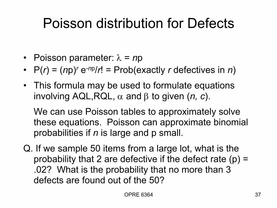
Poisson distribution for Defects
• Poisson parameter: λ = np• P(r) = (np)r e-np/r! = Prob(exactly r defectives in n)• This formula may be used to formulate equations
involving AQL,RQL, α and β to given (n, c).We can use Poisson tables to approximately solve these equations. Poisson can approximate binomial probabilities if n is large and p small.
Q. If we sample 50 items from a large lot, what is the probability that 2 are defective if the defect rate (p) = .02? What is the probability that no more than 3 defects are found out of the 50?

OPRE 6364 38
Hypergeometric Distribution• Hypergeometric formula:
r defectives in sample size n when M defectives are in N.• This distribution is used when sampling from a small
population. It is used when the lot size is not significantly greater than the sample size.
• (Can’t assume here each new part picked is unaffected by the earlier samples drawn).
Q. A lot of 20 tires contains 5 defective ones (i.e., p = 0.25).If an inspector randomly samples 4 items, what is the probability of 3 defective ones?
−−
=
Nn
Mr
MNrn
rP )(

OPRE 6364 39
Sampling Plan Design by Binomial Distribution
• Binomial distribution:P(x defectives in n) = [n!/(x!(n-x))!]px(1- p)n-x
Recall n!/(x!(n-x))! = ways to choose x in n
Q. If 4 samples (items) are chosen from a population with a defect rate = .1, what is the probability that
a) exactly 1 out of 4 is defective? b) at most 1 out of 4 is defective?

OPRE 6364 40
Solving for (n, c)
To design a single sampling plan we need two points. Typically these are p1 = AQL, p2 = LTPD and , are the Producer's Risk (Type I error) and Consumer's Risk (Type II error), respectively. By binomial formulas, n and c are the solution to
These two simultaneous equations are nonlinear so there is no simple, direct solution. The Larson nomogram can help us here.

OPRE 6364 41
The Larson Nomogram
● Applies to single sampling plan
● Based on binomial distribution
● Uses1-α = Pa at AQLβ = Pa at RQL
● Can produce OC curve

OPRE 6364 42
Definitions and TermsReference: NIST Engineering Statistics Handbook
Acceptable Quality Level (AQL): The AQL is a percent defective that is the base line requirement for the quality of the producer's product. The producer would like to design a sampling plan such that there is a high probability of accepting a lot that has a defect level less than or equal to the AQL.
Lot Tolerance Percent Defective (LTPD) also calledRQL (Rejection Quality Level): The LTPD is a designated high defect level that would be unacceptable to the consumer. The consumer would like the sampling plan to have a low probability of accepting a lot with a defect level as high as the LTPD.

OPRE 6364 43
Type I Error (Producer's Risk): This is the probability, for a given (n, c) sampling plan, of rejecting a lot that has a defect level equal to the AQL. The producer suffers when this occurs, because a lot with acceptable quality was rejected. The symbol is commonly used for the Type I error and typical values for range from 0.2 to 0.01.
Type II Error (Consumer's Risk): This is the probability, for a given (n, c) sampling plan, of accepting a lot with a defect level equal to the LTPD. The consumer suffers when this occurs, because a lot with unacceptable quality was accepted. The symbol is commonly used for the Type II error and typical values range from 0.2 to 0.01.

OPRE 6364 44
Operating Characteristic (OC) Curve: This curve plots the probability of accepting the lot (Y-axis) versus the lot fraction or percent defectives (X-axis).
The OC curve is the primary tool for displaying and investigating the properties of a sampling plan.

OPRE 6364 45
Average Outgoing Quality (AOQ): A common procedure, when sampling and testing is non-destructive, is to 100% inspect rejected lots and replace all defectives with good units. In this case, all rejected lots are made perfect and the only defects left are those in lots that were accepted. AOQ's refer to the long term defect level for this combined LASP and 100% inspection of rejected lots process. If all lots come in with a defect level of exactly p, and the OC curve for the chosen (n,c) LASP indicates a probability pa of accepting such a lot, over the long run the AOQ can easily be shown to be:
where N is the lot size.

OPRE 6364 46
Average Outgoing Quality Level (AOQL): A plot of the AOQ (Y-axis) versus the incoming lot p (X-axis) will start at 0 for p = 0, and return to 0 for p = 1 (where every lot is 100% inspected and rectified). In between, it will rise to a maximum. This maximum, which is the worst possible long term AOQ, is called the AOQL.
Average Total Inspection (ATI): When rejected lots are 100% inspected, it is easy to calculate the ATI if lots come consistently with a defect level of p. For a sampling plan (n, c) with a probability pa of accepting a lot with defect level p, we have
ATI = n + (1 - pa) (N - n)where N is the lot size.

OPRE 6364 47
Average Sample Number (ASN): For a single sampling plan (n, c) we know each and every lot has a sample of size n taken and inspected or tested. For double, multiple and sequential plans, the amount of sampling varies depending on the number of defects observed. For any given double, multiple or sequential plan, a long term ASNcan be calculated assuming all lots come in with a defect level of p. A plot of the ASN, versus the incoming defect level p, describes the sampling efficiency of a given lot sampling scheme.

OPRE 6364 48
The MIL-STD-105E approachA Query from a Practitioner: Selecting AQL (acceptable quality levels)I'd like some guidance on selecting an acceptable quality level and inspection levels when using sampling procedures and tables. For example, when I use MIL-STD-105E, how do I to decide when I should use GI, GII or S2, S4?
-- Confused in Columbus, OhioW. Edwards Deming observed that the main purpose of MIL-STD-105 was to beat the vendor over the head. "You cannot improve the quality in the process stream using this approach," cautions Don Wheeler, author of Understanding Statistical Process Control (SPC Press, 1992). "Neither can you successfully filter out the bad stuff. About the only place that this procedure will help is in trying to determine which batches have already been screened and which batches are raw, unscreened, run-of-the-mill bad stuff from your supplier. I taught these techniques for years but have repented of this error in judgment. The only appropriate levels of inspection are all or none. Anything else is just playing roulette with the product."
OPRE 6364 49
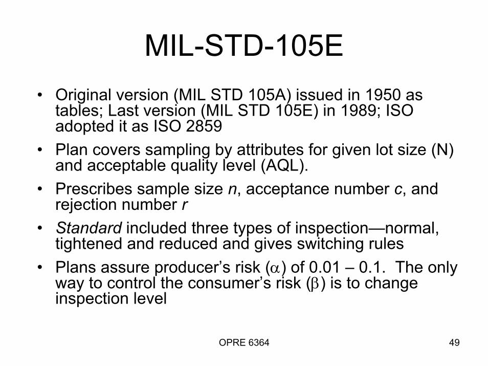
MIL-STD-105E• Original version (MIL STD 105A) issued in 1950 as
tables; Last version (MIL STD 105E) in 1989; ISO adopted it as ISO 2859
• Plan covers sampling by attributes for given lot size (N) and acceptable quality level (AQL).
• Prescribes sample size n, acceptance number c, and rejection number r
• Standard included three types of inspection—normal, tightened and reduced and gives switching rules
• Plans assure producer’s risk (α) of 0.01 – 0.1. The only way to control the consumer’s risk (β) is to change inspection level

OPRE 6364 50
AQL Acceptance Sampling by Attributes by MILSTD 105E
• Determine lot size N and AQL for the task at hand• Decide the type of sampling—single, double, etc.• Decide the state of inspection (e.g. normal)• Decide the type of inspection level (usually II)• Look at Table K for sample sizes• Look at the sampling plans tables (e.g. Table IIA)• Read n, Ac and Re numbers
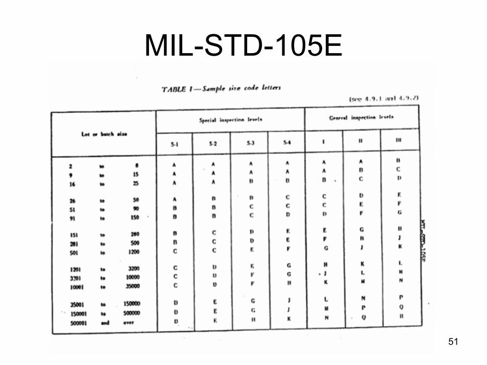
OPRE 6364 51
MIL-STD-105E

OPRE 6364 52

OPRE 6364 53
How/When would you use Acceptance Sampling?
• Advantages of acceptance sampling– Less handling damages– Fewer inspectors to put on payroll– 100% inspection costs are to high– 100% testing would take to long
• Acceptance sampling has some disadvantages– Risk included in chance of bad lot “acceptance” and
good lot “rejection”– Sample taken provides less information than 100%
inspection

OPRE 6364 54
Summary
• There are many basic terms you need to know to be able to understand acceptance sampling– SPC, Accept a lot, Reject a lot, Complete Inspection,
AQL, LTPD, Sampling Plans, Producer’s Risk, Consumer’s Risk, Alpha, Beta, Defect, Defectives, Attributes, Variables, ASN, ATI.

OPRE 6364 55
Useful links
http://www.bioss.sari.ac.uk/smart/unix/mseqacc/slides/frames.htmAcceptance Sampling Overview Text and Audio
http://iew3.technion.ac.il/sqconline/milstd105.htmlOnline calculator for acceptance sampling plans
http://www.stats.uwo.ca/courses/ss316b/2002/accept_02red.pdfAcceptance sampling mathematical background


