

HAL Id: hal-01552638https://hal.archives-ouvertes.fr/hal-01552638
Submitted on 6 Jul 2017
HAL is a multi-disciplinary open accessarchive for the deposit and dissemination of sci-entific research documents, whether they are pub-lished or not. The documents may come fromteaching and research institutions in France orabroad, or from public or private research centers.
L’archive ouverte pluridisciplinaire HAL, estdestinée au dépôt et à la diffusion de documentsscientifiques de niveau recherche, publiés ou non,émanant des établissements d’enseignement et derecherche français ou étrangers, des laboratoirespublics ou privés.
Acoustic distribution of discriminated micronektonicorganisms from a bi-frequency processing: the case
study of eastern Kerguelen oceanic watersNolwenn Béhagle, Cédric Cotté, Anne Lebourges-Dhaussy, Gildas Roudaut,
Guy Duhamel, Patrice Brehmer, Erwan Josse, Yves Cherel
To cite this version:Nolwenn Béhagle, Cédric Cotté, Anne Lebourges-Dhaussy, Gildas Roudaut, Guy Duhamel, et al..Acoustic distribution of discriminated micronektonic organisms from a bi-frequency processing: thecase study of eastern Kerguelen oceanic waters. Progress in Oceanography, Elsevier, 2017, 156, pp.276-289. �10.1016/j.pocean.2017.06.004�. �hal-01552638�

Acoustic distribution of discriminated micronektonic organisms from a bi-1
frequency processing: the case study of eastern Kerguelen oceanic waters 2
3
Nolwenn Béhaglea,b*, Cédric Cottéc, Anne Lebourges-Dhaussya, Gildas Roudauta, Guy 4
Duhameld, Patrice Brehmere, Erwan Jossea, Yves Cherelf 5
6
aIRD, UMR LEMAR 6539 (CNRS-IRD-IFREMER-UBO), BP70, 29280 Plouzané, France 7
bCNRS, UMR LOCEAN 7159 (CNRS-IRD-MNHN-UPMC), 4 place Jussieu, 75005 Paris, 8
France 9
cMNHN, UMR LOCEAN 7159 (CNRS-IRD-MNHN-UPMC), 4 place Jussieu, 75005 Paris, 10
France 11
dMNHN, UMR BOREA 7208(MNHN- CNRS-UPMC-IRD-UCBN-UAG), 43 rue Cuvier, CP 12
26,75231 Paris Cedex 05, France 13
eIRD, UMR 195 Lemar, ISRA-CRODT, Pole de Recherche de Hann, BP221, Dakar, Sénégal 14
fCNRS, UMR CEBC 7372 (CNRS-Université de La Rochelle), 79360 Villiers-en-Bois, France 15
16
*Corresponding author. E-mail address: [email protected] 17
18

Abstract 19
Despite its ecological importance, micronekton remains one of the least investigated 20
components of the open-ocean ecosystems. Our main goal was to characterize micronektonic 21
organisms using bi-frequency acoustic data (38 and 120 kHz) by calibrating an algorithm tool 22
that discriminates groups of scatterers in the top 300 m of the productive oceanic zone east of 23
Kerguelen Islands (Indian sector of the Southern Ocean). The bi-frequency algorithm was 24
calibrated from acoustic properties of mono-specific biological samples collected with trawls, 25
thus allowing to discriminate three acoustic groups of micronekton: (i) “gas-bearing” (∆Sv,120-26
38 < -1 dB), (ii) “fluid-like” (∆Sv,120-38 > 2 dB), and (iii) “undetermined” scatterers (-1 < ∆Sv,120-27
38 < 2 dB). The three groups likely correspond biologically to gas-filled swimbladder fish 28
(myctophids), crustaceans (euphausiids and hyperiid amphipods), and other marine organisms 29
potentially present in these waters and containing either lipid-filled or no inclusion (e.g. other 30
myctophids), respectively. The Nautical Area Scattering Coefficient (NASC) was used (echo-31
integration cells of 10m long and 1m deep) between 30 and 300m depth as a proxy of relative 32
biomass of acoustic targets. The distribution of NASC values showed a complex pattern 33
according to: (i) the three acoustically-defined groups, (ii) the type of structures (patch vs. 34
layers) and (iii) the timing of the day (day/night cycle). NASC values were higher at night 35
than during the day. A large proportion of scatterers occurred in layers while patches, that 36
mainly encompass gas-bearing organisms, are especially observed during daytime. This 37
method provided an essential descriptive baseline of the spatial distribution of micronekton 38
and a relevant approach to (i) link micronektonic group to physical parameters to define their 39
habitats, (ii) investigate trophic interactions by combining active acoustic and top predator 40
satellite tracking, and (iii) study the functioning of the pelagic ecosystems at various spatio-41
temporal scales. 42
43

Keywords: Euphausiid, Kerguelen, Myctophid, Southern Ocean, Acoustics. 44
1. Introduction 45
46
Micronektonic organisms (~1-20 cm in length; Kloser et al., 2009) constitute one of 47
the most noticeable and ecologically important components of the open ocean. They amount 48
to a substantial biomass (e.g. estimated at > 10 000 million metric tons of mesopelagic fish in 49
oceanic waters worldwide and ~380 million metric tons of Antarctic krill in the Southern 50
Ocean; Atkinson et al., 2009; Irigoien et al., 2014) with high nutritional value (Shaviklo and 51
Rafipour, 2013; Koizumi et al., 2014) leading to increasing commercial interest (Pauly et al., 52
1998). In oceanic waters, micronekton contribute to the export of carbon from the surface to 53
deeper layers (the biological pump) through extensive daily vertical mesopelagic migrations 54
to feed on near-surface organisms at night (Bianchi et al., 2013). They play a prominent role 55
in oceanic food webs by linking primary consumers to higher predators, including 56
commercially targeted fish species and oceanic squids, together with charismatic species, such 57
as marine mammals and seabirds (Rodhouse and Nigmatullin, 1996; Robertson and Chivers, 58
1997; Potier et al. 2007; Spear et al. 2007). Despite their ecological importance, micronekton 59
remain one of the least investigated components of the marine ecosystems, with major gaps in 60
our knowledge of their biology, ecology, and major uncertainties about their global biomass 61
(Handegard et al., 2013; Irigoien et al., 2014). 62
Acoustic methods have been used in fishery operations and research since 1935 (Sund, 63
1935). Stock assessment drove a continuous improvement of the methods in order to better 64
investigate the distribution and abundance of targeted marine organisms (Simmonds and 65
MacLennan, 2005). Beyond stock assessment, acoustics now extends to whole marine 66
ecosystems, being the best available tool allowing simultaneous collection of qualitative and 67
quantitative data on their biotic and even abiotic components (Bertrand et al., 2013). A major 68
limitation of acoustics is the lack of accurate taxonomic information about the ensonified 69

organisms. Hence, acoustic analytical tools to determine characteristics of biological 70
backscatters were developed by comparing and quantifying the difference of mean volume 71
backscattering strength between different frequencies. The rationale is that the acoustic 72
properties of individual species are known to vary with the operating frequencies of the echo 73
sounder. For example, both experimental and theoretical studies showed large variations in 74
the average echo energy per unit biomass due to animals from “fluid-like” to “elastic shelled” 75
organisms (Stanton et al., 1994, 1998a, 1998b). This approach has been used since the late 76
1970s to identify and quantify zooplanktonic scatterers (Greenlaw, 1977; Holliday and Pieper, 77
1980; Madureira et al., 1993a,b). Less has been done to characterize micronektonic organisms 78
from the open sea, where micronekton are diverse and include small pelagic fishes, 79
cephalopods, large crustaceans and gelatinous animals. A recent biomass estimate of mid-80
water fish was based on the 38 kHz frequency alone (Irigoien et al., 2014). Furthermore, the 81
difference of mean volume backscattering strength between two frequencies (38 and 120 kHz) 82
was used to differentiate “fish”, “macrozooplankton” and “zooplankton” scatterers (Fielding 83
et al., 2012; Bedford et al., 2015). 84
In the Southern Ocean (water masses south of the Subtropical Front), the importance 85
of micronekton is illustrated by the considerable populations of subantarctic seabirds and 86
pinnipeds that primarily prey on schooling myctophids, swarming euphausiids and hyperiid 87
amphipods (Cooper and Brown, 1990; Woehler and Green, 1992; Guinet et al., 1996; Bocher 88
et al., 2001). However, to our knowledge, acoustic investigation of mid-water organisms in 89
lower latitudes of the Southern Ocean is limited to a few surveys (Miller, 1982; Perissinotto 90
and McQuaid 1992; Pakhomov and Froneman, 1999), and only three recent studies 91
discriminated acoustic groups by their bi-frequency characteristics (Fielding et al., 2012; 92
Saunders et al., 2013; Bedford et al., 2015). 93

The main goal of the present work was to use bi-frequency acoustic data (38 and 120 94
kHz) combined with net sampling to calibrate an algorithm tool that discriminates groups of 95
scatterers in an acoustically poorly-explored area. The targeted region was the productive 96
oceanic zone off south-eastern Kerguelen Islands, because: (i) several significant populations 97
of predators are known to feed on micronektonic organisms in the area during the summer 98
months, namely Antarctic fur seals and king penguins on mesopelagic fishes (mainly 99
myctophids) and macaroni penguins on euphausiids and hyperiids (Bost et al., 2002; 100
Charrassin et al., 2004; Lea et al., 2002; C.A. Bost and Y. Cherel, unpublished data); and (ii) 101
myctophid fishes and euphausiids were already successfully collected in the area (Duhamel et 102
al., 2000, 2005; authors’ unpublished data). The rationale was that different groups of 103
micronektonic organisms (large crustaceans and mid-water fish) should be abundant in the 104
targeted area and that the bi-frequency acoustic data should allow investigating their 105
horizontal and vertical abundance patterns according to the type of structures (patches and 106
layers). 107
2. Materials and methods 108
109
The oceanographic cruise (MD197/MYCTO) was carried out during the austral 110
summer 2013-2014 on board the R/V Marion Dufresne II. The overall dataset was based on 111
1,320 km of acoustic data in oceanic waters off Kerguelen Islands during 14 consecutive days 112
of recording. 113
114
2.1. Acoustic sampling 115
In situ acoustic data were recorded day and night during the period 23 January-5 116
February 2014. Measurements were made when cruising at a speed of 8 knots, using a Simrad 117
EK60 split-beam echo sounder operating simultaneously at 38 and 120 kHz. The transducers 118
were hull-mounted at a depth of 6 m below the water surface. An offset of 30 m below the 119
surface was applied to account for: (i) the depth of the transducers, (ii) the acoustic Fresnel 120
zone, and (iii) the acoustic interference from surface turbulence. Acoustic data were thus 121
collected on a vertical range from 30 to 300 m according to the 120 kHz range (Fig. 1). The 122
limited depth of 300m is considered in the interpretation of mid-water organisms 123
distributions, especially for those which are known to perform vertical migration according to 124
the day/night cycle (diel vertical migration; Lebourges‐Dhaussy et al., 2000; Benoit‐Bird et 125
al., 2009) (see section 4.2 below). Indeed, most of these organisms were sampled at night but 126
only epipelagic and some mesopelagic organisms were observable during the day within this 127
depth range. 128
129
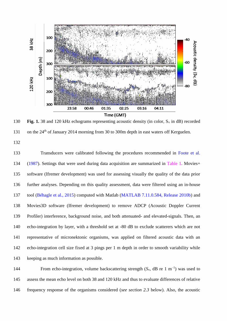
Fig. 1. 38 and 120 kHz echograms representing acoustic density (in color, Sv in dB) recorded 130
on the 24th of January 2014 morning from 30 to 300m depth in east waters off Kerguelen. 131
132
Transducers were calibrated following the procedures recommended in Foote et al. 133
(1987). Settings that were used during data acquisition are summarized in Table 1. Movies+ 134
software (Ifremer development) was used for assessing visually the quality of the data prior 135
further analyses. Depending on this quality assessment, data were filtered using an in-house 136
tool (Béhagle et al., 2015) computed with Matlab (MATLAB 7.11.0.584, Release 2010b) and 137
Movies3D software (Ifremer development) to remove ADCP (Acoustic Doppler Current 138
Profiler) interference, background noise, and both attenuated- and elevated-signals. Then, an 139
echo-integration by layer, with a threshold set at -80 dB to exclude scatterers which are not 140
representative of micronektonic organisms, was applied on filtered acoustic data with an 141
echo-integration cell size fixed at 3 pings per 1 m depth in order to smooth variability while 142
keeping as much information as possible. 143
From echo-integration, volume backscattering strength (Sv, dB re 1 m–1) was used to 144
assess the mean echo level on both 38 and 120 kHz and thus to evaluate differences of relative 145
frequency response of the organisms considered (see section 2.3 below). Also, the acoustic 146
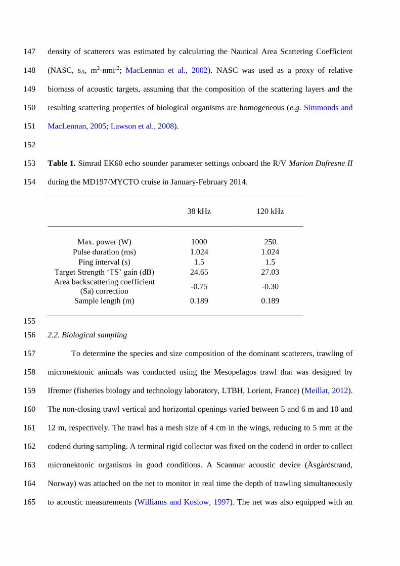
density of scatterers was estimated by calculating the Nautical Area Scattering Coefficient 147
(NASC, sA, m2·nmi‐2; MacLennan et al., 2002). NASC was used as a proxy of relative 148
biomass of acoustic targets, assuming that the composition of the scattering layers and the 149
resulting scattering properties of biological organisms are homogeneous (e.g. Simmonds and 150
MacLennan, 2005; Lawson et al., 2008). 151
152
Table 1. Simrad EK60 echo sounder parameter settings onboard the R/V Marion Dufresne II 153
during the MD197/MYCTO cruise in January-February 2014. 154
38 kHz 120 kHz
Max. power (W) 1000 250
Pulse duration (ms) 1.024 1.024
Ping interval (s) 1.5 1.5
Target Strength ‘TS’ gain (dB) 24.65 27.03
Area backscattering coefficient
(Sa) correction -0.75 -0.30
Sample length (m) 0.189 0.189
155
2.2. Biological sampling 156
To determine the species and size composition of the dominant scatterers, trawling of 157
micronektonic animals was conducted using the Mesopelagos trawl that was designed by 158
Ifremer (fisheries biology and technology laboratory, LTBH, Lorient, France) (Meillat, 2012). 159
The non-closing trawl vertical and horizontal openings varied between 5 and 6 m and 10 and 160
12 m, respectively. The trawl has a mesh size of 4 cm in the wings, reducing to 5 mm at the 161
codend during sampling. A terminal rigid collector was fixed on the codend in order to collect 162
micronektonic organisms in good conditions. A Scanmar acoustic device (Åsgårdstrand, 163
Norway) was attached on the net to monitor in real time the depth of trawling simultaneously 164
to acoustic measurements (Williams and Koslow, 1997). The net was also equipped with an 165
elephant seal tag (Sea Mammal Research Unit, UK) that was fixed on the trawl headline. The 166
tag was a multisensor data logger recording pressure (accuracy of 2 dbar) and hence depth, 167
temperature, salinity and fluorescence (Blain et al., 2013). Only depth data were analyzed in 168
the present work, thus providing an accurate time/depth profile for each tow. The trawl was 169
towed for 30 min at targeted depth at a speed of 1.5-2.5 knots. All catches were sorted by 170
species or lowest identifiable taxonomic groups, measured and weighed. While Antarctic krill 171
(Euphausia superba) does not occur in the area, collected taxa were representative of the 172
Polar Frontal Zone and Polar Front, including zooplankton-like organisms (i.e. euphausiids, 173
amphipods, large copepods and non-gaseous gelatinous organisms), fish-like organisms (i.e. 174
fish with a gas-filled swimbladder and gaseous gelatinous organisms), and other organisms 175
(i.e. fish without a gas-filled swimbladder and small squids). Most of the 39 pelagic hauls 176
conducted during this survey had mixed catches and were not further considered here. Indeed, 177
to be able to calibrate as correctly as possible a bi-frequency algorithm in this area, we chose 178
to use only mono-specific trawls. Two trawls were suitable for acoustic mark identification, 179
because almost all the catches consisted of one single species in large quantity (see section 2.3 180
below). 181
182
2.3. Bi-frequency method calibration 183
The acoustic properties of biological organisms vary with the operating frequency of 184
the echo sounder. Therefore, comparing the echo levels of individual scatterers ensonified at 185
different frequencies is likely to provide information on the types of targets that are present in 186
the water column (Madureira et al., 1993a,b; Kang et al., 2002). According to the literature, 187
zooplankton-like and non-gaseous gelatinous organisms have an increasing relative frequency 188
response between 38 and 120 kHz (Stanton and Chu, 2000; David et al., 2001; Lavery et al., 189
2002; Korneliussen and Ona, 2003), whereas fish with a gas-filled swimbladder and gaseous 190
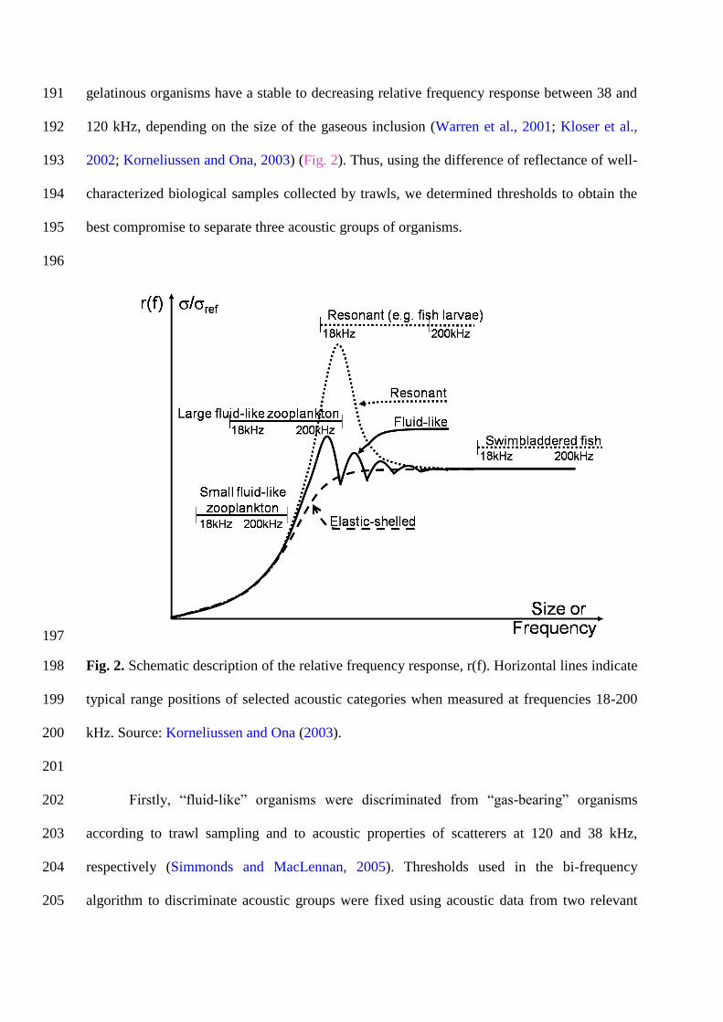
gelatinous organisms have a stable to decreasing relative frequency response between 38 and 191
120 kHz, depending on the size of the gaseous inclusion (Warren et al., 2001; Kloser et al., 192
2002; Korneliussen and Ona, 2003) (Fig. 2). Thus, using the difference of reflectance of well-193
characterized biological samples collected by trawls, we determined thresholds to obtain the 194
best compromise to separate three acoustic groups of organisms. 195
196
197
Fig. 2. Schematic description of the relative frequency response, r(f). Horizontal lines indicate 198
typical range positions of selected acoustic categories when measured at frequencies 18-200 199
kHz. Source: Korneliussen and Ona (2003). 200
201
Firstly, “fluid-like” organisms were discriminated from “gas-bearing” organisms 202
according to trawl sampling and to acoustic properties of scatterers at 120 and 38 kHz, 203
respectively (Simmonds and MacLennan, 2005). Thresholds used in the bi-frequency 204
algorithm to discriminate acoustic groups were fixed using acoustic data from two relevant 205

trawls, which were selected according to: (i) their depth (only trawls between the surface and 206
200 m depth were considered to minimize as much as possible interference from the saturated 207
outgoing signal at 120 kHz), and (ii) the quality of their acoustic data (mainly depending on 208
the weather; only trawls with more than 50% of clean pings were considered). Two night 209
trawls (T07, 50 m depth and T14, 70 m depth) were mono-specific in their composition, 210
containing almost exclusively adults of subantarctic krill Euphausia vallentini (15-24 mm 211
long) and juveniles of the demersal fish Muraenolepis marmoratus (31-40 mm long), 212
respectively. The latter corresponds to the pelagic stage of the species (Duhamel et al., 2005), 213
i.e. fish were 3-4 cm long and contained a well-developed gas-filled swimbladder, similar to 214
several species of myctophids (Electrona carlsbergi, Krefftichthys anderssoni, 215
Protomyctophum spp.; Saunders et al., 2013). The acoustic characteristics of samples from 216
these two trawl tows were considered as representative of “fluid-like” and “gas-bearing” 217
scatterers, respectively. Only the acoustic characteristics corresponding in time and depth to 218
the two trawls were taken into account to grade the bi-frequency algorithm in order to be sure 219
that they were related to the organisms effectively caught in the net. For doing this, we used 220
the time/depth data provided by the elephant seal tag for extracting the acoustic data from 2 m 221
above the headline up to 10 m below (or 2 m below the footrope) during a limited time period 222
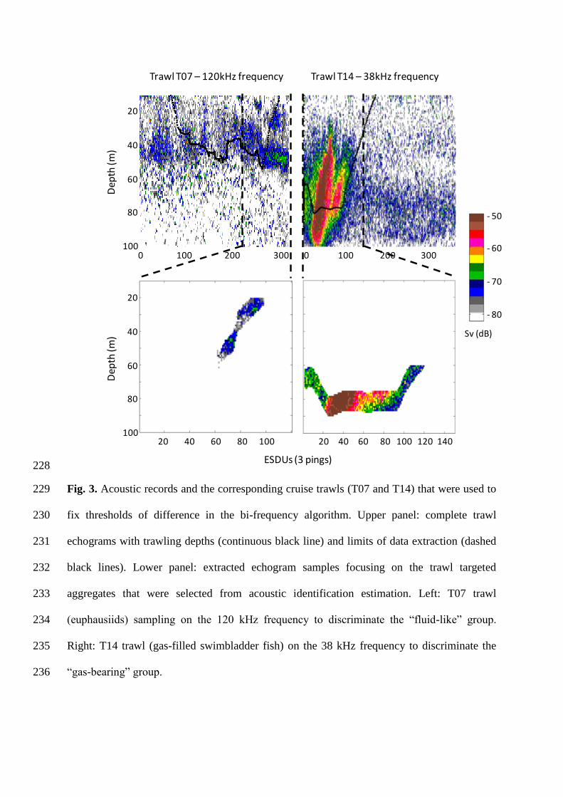
that focused on the acoustically detected aggregations (Fig. 3). The acoustic response at 38 223
and 120 kHz, of each echo-integration cell belonging to the trawl’s path, was represented 224
relative to the 38 kHz frequency (Fig. 4a) to assess the positive vs. negative slope of the 225
relative frequency response between discrete 38 and 120 kHz frequencies. 226
227
20
40
60
80
100
Dep
th (m
)
20 40 60 80 100 20 40 60 80 100 120 140
ESDUs (3 pings)
Trawl T07 – 120kHz frequency Trawl T14 – 38kHz frequency
20
40
60
80
100
Dep
th (m
)
0 100 200 300 0 100 200 300
- 80
- 70
- 60
- 50
Sv (dB)
228
Fig. 3. Acoustic records and the corresponding cruise trawls (T07 and T14) that were used to 229
fix thresholds of difference in the bi-frequency algorithm. Upper panel: complete trawl 230
echograms with trawling depths (continuous black line) and limits of data extraction (dashed 231
black lines). Lower panel: extracted echogram samples focusing on the trawl targeted 232
aggregates that were selected from acoustic identification estimation. Left: T07 trawl 233
(euphausiids) sampling on the 120 kHz frequency to discriminate the “fluid-like” group. 234
Right: T14 trawl (gas-filled swimbladder fish) on the 38 kHz frequency to discriminate the 235
“gas-bearing” group. 236

237
Secondly, the difference in relative frequency response (∆Sv,120-38 = Sv,120 – Sv,38) was 238
evaluated per echo-integration cell using a varying threshold of difference, ranging from -15 239
to 25 dB (Fig. 4b). For each threshold considered one by one, each acoustic sample was 240
classified either in a group “lower than the threshold considered” or in the opposite group 241
“higher than the threshold considered”. The total acoustic density was calculated (on 120 kHz 242
samples for the “fluid-like” group and on 38 kHz samples for the “gas-bearing” group) for 243
each of the lower/higher groups formed and reported in percentage to total acoustic density of 244
the aggregate for each tested threshold (Fig. 4b). 245
246
Fig. 4. Left panel (a): frequency response of each sample considered relatively to the 38 kHz 247
frequency, with "fluid-like" samples (from the trawl T07) represented in red and "gas-248
bearing" samples (from the trawl T14) in blue. Right panel (b): bar chart of the percentage of 249
"fluid-like" (in red) and "gas-bearing" (in blue) total NASC, according to a -15 to 25 dB range 250
of threshold of difference, used to define the best thresholds (-1 and +2 dB) delimiting the 251
“undetermined” group by transferring a maximum of 10% of their acoustic energy (total 252
NASC). 253
254

Finally, the calculated “loss” of density for both “fluid-like” and “gas-bearing” groups 255
was used to define two thresholds of differences delimiting the “undetermined” group by 256
transferring a maximum of 10% of their acoustic energy (Fig. 4b) into the “undetermined” 257
group. This group corresponds to an uncertainty zone where scatterers (i) have a close-to-flat 258
relative frequency response between discrete 38 and 120 frequencies, (ii) cannot be allocated 259
to “fluid-like” or “gas-bearing” organisms according to their Sv difference measured between 260
38 and 120 kHz but (iii) are potentially present in the water column and (iv) have no 261
biological validation in this work. Preserving such a group allows accounting for organisms 262
that could not be identified during this work from biological sampling but are present in the 263
water column, while being more demanding on well-defined groups. Following this method, 264
thresholds were defined at -1 and +2 dB. Scatterers with ∆Sv,120-38 (i) > +2 dB are classified in 265
the “fluid-like” group, (ii) < -1 dB are classified in the “gas-bearing” group and (iii) between -266
1 and +2 dB are classified in a third “undetermined” group (Fig. 5). 267
268
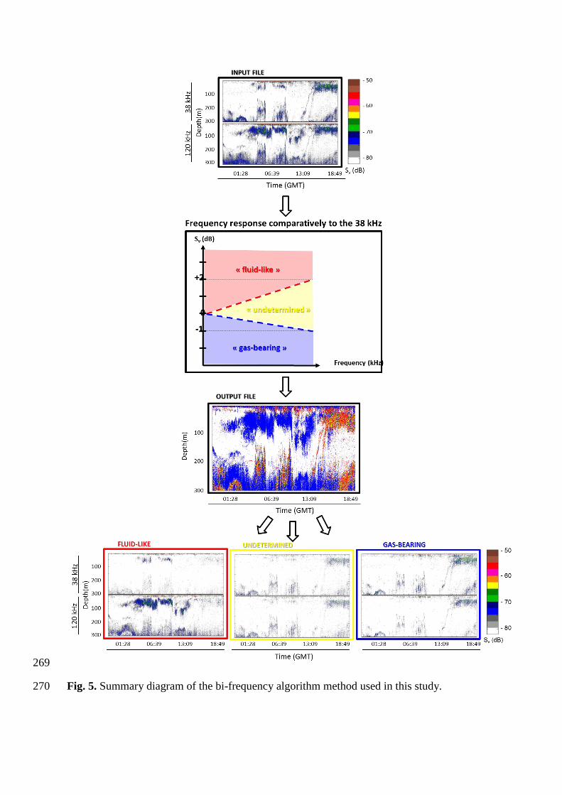
269
Fig. 5. Summary diagram of the bi-frequency algorithm method used in this study. 270

2.4. Testing the bi-frequency algorithm 271
The robustness of threshold values obtained by the bi-frequency algorithm developed 272
in the present work was tested by calculating the theoretical frequency responses of 273
Muraenolepis marmoratus and Euphausia vallentini using the mathematical models of Ye 274
(1997) and Stanton et al. (1994), respectively. While the Ye model provides an analytic 275
method for studying scattering of “gas-bearing” organisms at low frequencies, the Stanton 276
model focuses on the “fluid-like” organisms’ acoustic properties. 277
The Ye (1997) model highlights a ∆Sv,120-38 value of -0.4 dB for fish of 3 to 4 cm 278
length (as sampled during the T14 trawl), and the Stanton et al. (1994) model for randomly-279
oriented fluid, bent cylinder highlights a ∆Sv,120-38 value of +1.9 dB for euphausiids of 15-24 280
mm length (length range of organisms sampled during the T07 trawl). Using the bi-frequency 281
algorithm, the ∆Sv,120-38 thresholds amounted to -1 and +2 dB, respectively, and are thus 282
consistent with the results of mathematical models. Our threshold values were even stronger 283
than those of the models (-1 < -0.4 and 2 > 1.9 dB), thus highlighting the selectivity of the 284
algorithm. According to biological samples (see section 2.2. above) and acoustic properties of 285
scatterers at 38 and 120 kHz (see section 2.3 above), three acoustic groups have been defined 286
for micronektonic organisms: (i) “gas-bearing” (∆Sv,120-38 < -1 dB), (ii) “fluid-like” (∆Sv,120-38 287
> 2 dB), and (iii) “undetermined” scatterers (-1 < ∆Sv,120-38 < 2 dB). 288
289
2.5. Data post-processing and statistical analyses 290
Each echo-integration cell was attributed to “fluid-like”, “undetermined” or “gas-291
bearing” group based on its relative frequency response. Moreover, as living organisms 292
follow non-random and non-uniform distributions (Margalef, 1979; Legendre and Fortin, 293
2004), acoustic data were analyzed separately in terms of patches and layers. 294

First of all, in order to get homogenous horizontal sampling at high resolution, filtered 295
data at 38 and 120 kHz have been echo integrated in cells of 10 m (horizontal) by 1 m 296
(vertical). Patches were here defined as isolated groups of echo-integrated cells limited in 297
space (between 10 and 3000 m long) and associated to a mean volume backscattering strength 298
Sv ≥ -63 dB on the mean 38 and 120 kHz echogram. In contrast, layers were defined as 299
continuous and homogenous areas of acoustic detections with a mean Sv < -63 dB for each 300
echo-integrated cell on the mean 38 and 120 kHz echogram. The -63 dB threshold was 301
defined by the operator after a visual analysis of the number of patches detected along a 302
representative acoustic sample of five hours long and along increasing Sv values from -70 to -303
40 dB. The value of -63 dB corresponds to a threshold level over which the number of patches 304
did not further increased (Fig. 6). 305
306
Fig. 6. Representative diagram of the number of patches (in blue) and its derivative (in green) 307
detected along increasing Sv values from -70 to -40 dB. The value of -63 dB corresponds to a 308
threshold level over which the number of patches did not further increased. 309
310
Nu
mb
er o
f p
atch
es
2000
1500
1000
500
0
0
1000
Derivated
nu
mb
er of p
atches
Mean volume backscattering strength (Sv, in dB)
-70 -65 -60 -55 -50 -45 -40-63

Using the Matlab contouring tool, echo-integrated cells having a mean Sv ≥ -63 dB 311
were extracted from the echo integrated datasets and each contour considered as a detected 312
patch (Fig. 7a). For each patch, mean depth, vertical size, mean Sv and mean NASC values at 313
both frequencies were computed. NASC values were first summed on the vertical and then 314
averaged on the horizontal. Cells that were not considered as patches were considered as 315
layers (Fig. 7b). 316
317
Fig. 7. 38 and 120 kHz echograms representing acoustic density (in color, Sv in dB) recorded 318
on the 24th of January 2014 morning from 30 to 300m depth in east waters off Kerguelen for 319
(a) patches- and (b) layers structures. 320

Total-, patches- and layers- datasets were then post-processed following the same bi-321
frequency algorithm (see section 2.3 above). Thus, nine datasets were obtained: “fluid-like”, 322
“gas-bearing”, and “undetermined” for layer structures, for patch structures, and for the whole 323
(i.e. patches and layers together). 324
Acoustic data were analyzed from 30 to 300 m depth according to the applied offset 325
(see section 2.1. above) and the 120 kHz emission range. Day and night data were analyzed 326
separately because many mid-water organisms undergo diel vertical migration. The 327
crepuscular period (45 minutes before and after sunrise and sunset) during which mid-water 328
organisms ascend and descend (Lebourges‐Dhaussy et al., 2000; Benoit‐Bird et al., 2009) 329
were excluded from the analyses. 330
Statistical analyses were performed within the R environment (R Core Team, 2014). 331
Differences of distribution between groups were statistically assessed using student t tests. 332
3. Results 333
334
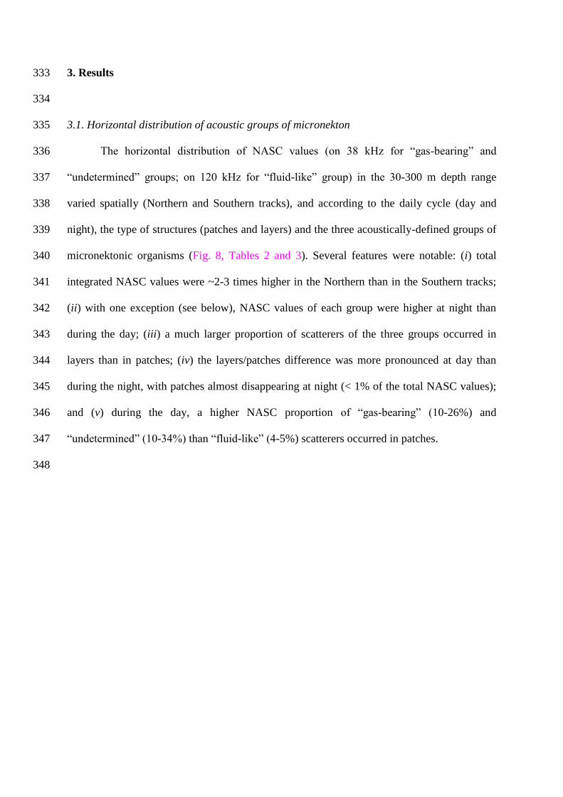
3.1. Horizontal distribution of acoustic groups of micronekton 335
The horizontal distribution of NASC values (on 38 kHz for “gas-bearing” and 336
“undetermined” groups; on 120 kHz for “fluid-like” group) in the 30-300 m depth range 337
varied spatially (Northern and Southern tracks), and according to the daily cycle (day and 338
night), the type of structures (patches and layers) and the three acoustically-defined groups of 339
micronektonic organisms (Fig. 8, Tables 2 and 3). Several features were notable: (i) total 340
integrated NASC values were ~2-3 times higher in the Northern than in the Southern tracks; 341
(ii) with one exception (see below), NASC values of each group were higher at night than 342
during the day; (iii) a much larger proportion of scatterers of the three groups occurred in 343
layers than in patches; (iv) the layers/patches difference was more pronounced at day than 344
during the night, with patches almost disappearing at night (< 1% of the total NASC values); 345
and (v) during the day, a higher NASC proportion of “gas-bearing” (10-26%) and 346
“undetermined” (10-34%) than “fluid-like” (4-5%) scatterers occurred in patches. 347
348

349
Fig. 8. Total density (NASC, scaled in m²·nmi-2, colored on ship track) observed during the cruise integrated from 30 to 300 m depth for each 350
acoustic group (“gas-bearing”, fluid-like” and “undetermined” groups) and for each type of structure (patches and layers). 351

Table 2. Acoustic density (NASC, in m²·nmi-2) per echo-integration cell of each acoustic group (“gas-bearing”, “fluid-like” and “undetermined” 352
groups). Values are means ± SD. The small size of the 10 m horizontal cells explains both their numbers and very large variances. 353
354
Time period Tracks Echo-integration
cell per 10 m (n) Total NASC values at
38 or 120 Hz (m²·nm-2) "Fluid-like" NASC values
at 120 kHz (m²·nm-2) "Gas-bearing" NASC
values at 38 kHz (m²·nm-2) "Undetermined" NASC
values at 38 kHz (m²·nm-2)
Day Northern 69150 446 ± 3402 283 ± 2641 107 ± 1073 56 ± 756
Southern 37724 273 ± 1642 209 ± 1507 42 ± 563 22 ± 136
Both tracks 106874 385 ± 2907 257 ± 2305 84 ± 372 44 ± 614
Night Northern 15252 649 ± 3091 351 ± 2432 225 ± 1487 73 ± 454
Southern 5065 195 ± 579 73 ± 431 84 ± 372 38 ± 32
Both tracks 20317 536 ± 2701 282 ± 2122 190 ± 1303 64 ± 394
Day and night Northern 84402 483 ± 3349 295 ± 2604 129 ± 1160 59 ± 711
Southern 42789 264 ± 1555 193 ± 1423 47 ± 544 24 ± 128
Both tracks 127191 409 ± 2875 261 ± 2277 101 ± 998 47 ± 584
355
356
357
358
359
360
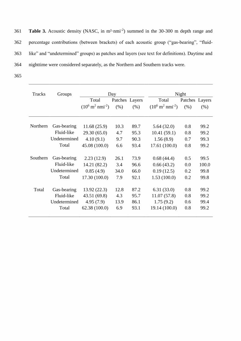
Table 3. Acoustic density (NASC, in m²·nmi-2) summed in the 30-300 m depth range and 361
percentage contributions (between brackets) of each acoustic group (“gas-bearing”, “fluid-362
like” and “undetermined” groups) as patches and layers (see text for definitions). Daytime and 363
nighttime were considered separately, as the Northern and Southern tracks were. 364
365
Tracks Groups Day Night
Total Patches Layers Total Patches Layers
(106 m2 nmi-2) (%) (%) (106 m2 nmi-2) (%) (%)
Northern Gas-bearing 11.68 (25.9) 10.3 89.7 5.64 (32.0) 0.8 99.2
Fluid-like 29.30 (65.0) 4.7 95.3 10.41 (59.1) 0.8 99.2
Undetermined 4.10 (9.1) 9.7 90.3 1.56 (8.9) 0.7 99.3
Total 45.08 (100.0) 6.6 93.4 17.61 (100.0) 0.8 99.2
Southern Gas-bearing 2.23 (12.9) 26.1 73.9 0.68 (44.4) 0.5 99.5
Fluid-like 14.21 (82.2) 3.4 96.6 0.66 (43.2) 0.0 100.0
Undetermined 0.85 (4.9) 34.0 66.0 0.19 (12.5) 0.2 99.8
Total 17.30 (100.0) 7.9 92.1 1.53 (100.0) 0.2 99.8
Total Gas-bearing 13.92 (22.3) 12.8 87.2 6.31 (33.0) 0.8 99.2
Fluid-like 43.51 (69.8) 4.3 95.7 11.07 (57.8) 0.8 99.2
Undetermined 4.95 (7.9) 13.9 86.1 1.75 (9.2) 0.6 99.4
Total 62.38 (100.0) 6.9 93.1 19.14 (100.0) 0.8 99.2
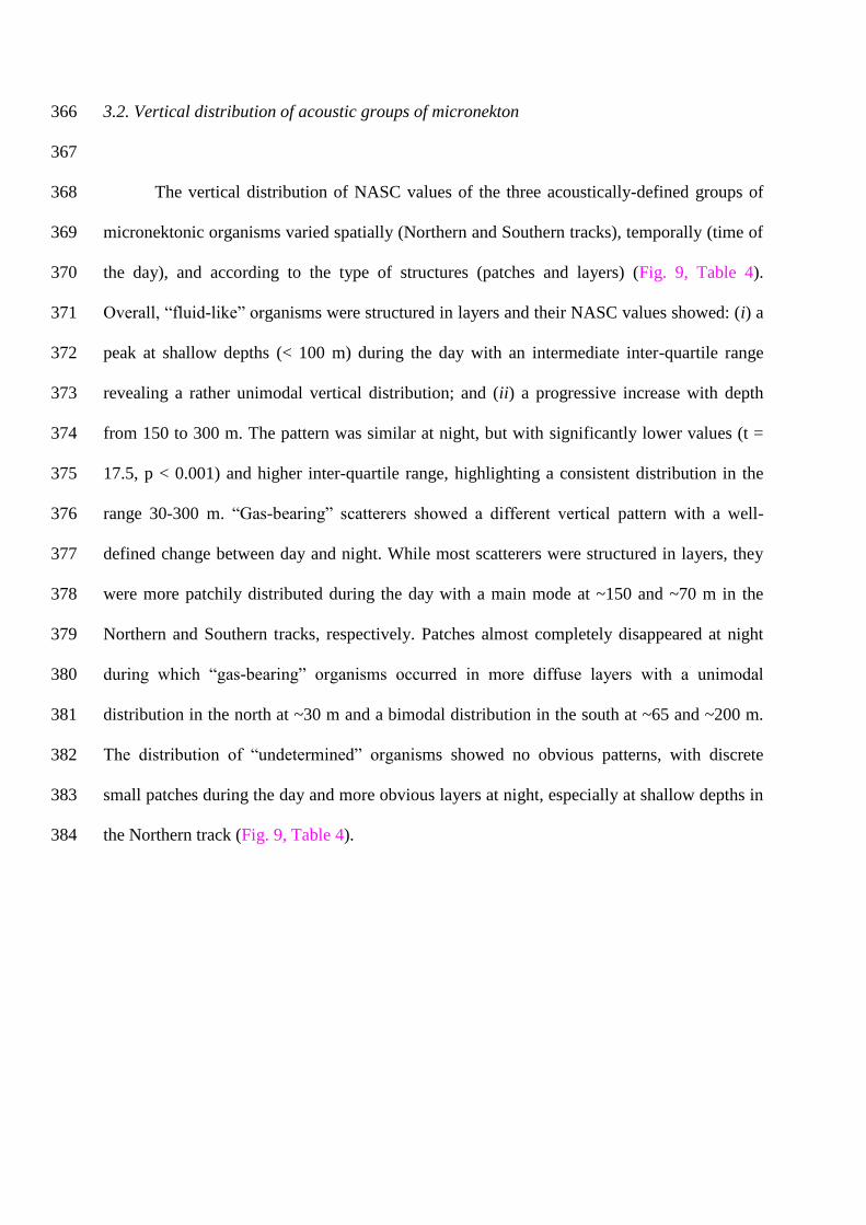
3.2. Vertical distribution of acoustic groups of micronekton 366
367
The vertical distribution of NASC values of the three acoustically-defined groups of 368
micronektonic organisms varied spatially (Northern and Southern tracks), temporally (time of 369
the day), and according to the type of structures (patches and layers) (Fig. 9, Table 4). 370
Overall, “fluid-like” organisms were structured in layers and their NASC values showed: (i) a 371
peak at shallow depths (< 100 m) during the day with an intermediate inter-quartile range 372
revealing a rather unimodal vertical distribution; and (ii) a progressive increase with depth 373
from 150 to 300 m. The pattern was similar at night, but with significantly lower values (t = 374
17.5, p < 0.001) and higher inter-quartile range, highlighting a consistent distribution in the 375
range 30-300 m. “Gas-bearing” scatterers showed a different vertical pattern with a well-376
defined change between day and night. While most scatterers were structured in layers, they 377
were more patchily distributed during the day with a main mode at ~150 and ~70 m in the 378
Northern and Southern tracks, respectively. Patches almost completely disappeared at night 379
during which “gas-bearing” organisms occurred in more diffuse layers with a unimodal 380
distribution in the north at ~30 m and a bimodal distribution in the south at ~65 and ~200 m. 381
The distribution of “undetermined” organisms showed no obvious patterns, with discrete 382
small patches during the day and more obvious layers at night, especially at shallow depths in 383
the Northern track (Fig. 9, Table 4). 384

385
Fig. 9. Mean vertical NASC profiles from 30 to 300 m depth of each acoustic group (“gas-386
bearing”, fluid-like” and “undetermined” groups) for day (black lines) and night (grey lines) 387
and for each type of structures (patches and layers). Dashed lines indicate the 95% confidence 388
intervals. 389

Table 4. Maximum acoustic density (NASC) depth, median acoustic density and inter-390
quantile range proportion of acoustic groups (calculated on the 38 kHz for the “gas-bearing” 391
and “undetermined” groups and on the 120 kHz for the “fluid-like” group) according to the 392
tracks (Northern and Southern), time of the day (day and night) and type of structures 393
(patches and layers). 394
Timing Tracks Groups Maximum NASC Median NASC values Inter-quantile depth (m) (m2 nmi-2) range (%)
Total
Day Northern Gas-bearing 148 0.16 24.6 Fluid-like 66 0.36 23.9 Undetermined 147 0.09 50.0 Southern Gas-bearing 72 0.11 19.3 Fluid-like 275 0.23 47.7 Undetermined 270 0.05 54.5
Night Northern Gas-bearing 42 0.13 27.3 Fluid-like 295 0.20 50.0 Undetermined 45 0.10 33.3 Southern Gas-bearing 65 0.23 34.7 Fluid-like 294 0.13 54.3 Undetermined 214 0.12 25.0
Patches
Day Northern Gas-bearing 147 0.03 10.4 Fluid-like 109 0.05 17.1 Undetermined 143 0.02 30.0 Southern Gas-bearing 68 0.01 9.7 Fluid-like 163 0.02 36.4 Undetermined 194 0.01 27.8
Night Northern Gas-bearing 45 0.00 7.1 Fluid-like 122 0.00 0.0 Undetermined 41 0.00 0.0 Southern Gas-bearing 94 0.00 0.0 Fluid-like 38 0.00 0.0 Undetermined 58 0.00 0.0
Layers
Day Northern Gas-bearing 230 0.13 59.3 Fluid-like 65 0.31 32.9 Undetermined 297 0.04 53.8 Southern Gas-bearing 263 0.07 54.2 Fluid-like 292 0.21 39.7 Undetermined 297 0.02 46.2
Night Northern Gas-bearing 42 0.14 27.7 Fluid-like 294 0.22 45.3 Undetermined 45 0.09 36.6 Southern Gas-bearing 65 0.28 33.3 Fluid-like 294 0.19 53.7 Undetermined 214 0.10 27.6

4. Discussion 395
396
Historically, most of the acoustic investigations conducted in the Southern Ocean 397
since the 1960s focused on Antarctic krill (Demer and Conti, 2005; Fielding et al., 2014), due 398
to its high and variable biomass (Atkinson et al., 2009), key role in the high-latitude pelagic 399
ecosystem (Ainley and DeMaster, 1990) and developing commercial fisheries (Nicol et al., 400
2012). More recently, the concept of a distinct Antarctic open-ocean food chain where 401
Antarctic krill is absent pointed out the importance of other micronektonic organisms, 402
including mid-water fish (Rodhouse and White, 1995). Hence, different groups were 403
acoustically characterized in the Antarctic krill zone (Fielding et al., 2012; Saunders et al., 404
2013), but, to our knowledge, little acoustic information is available in Northern waters of the 405
Southern Ocean where Antarctic krill is ecologically replaced by other micronektonic 406
organisms, namely euphausiids, a few hyperiid amphipods and myctophid fishes. 407
The present study focused on productive waters off eastern Kerguelen Islands, where 408
numerous top predators target micronektonic organisms different from Antarctic krill (Guinet 409
et al. 1996). It provides a first depiction of horizontal and vertical (30-300 m) distribution and 410
abundance of three different acoustic groups of micronektonic organisms from a bi-frequency 411
processing of acoustic data (38 and 120 kHz). 412
413
4.1. Methodological comments and biological interpretation of the acoustic groups 414
415
Methodologically, the frequency-dependent technique based on estimated differences 416
between mean volume-backscattering strength at 38 and 120 kHz has also previously been 417
used to characterize acoustic groups (Madureira 1993a,b; Brierley et al., 1998). The most 418
recent investigations defined two micronektonic groups in Antarctic waters, namely Antarctic 419

krill (macrozooplankton) that was identified using a 2-12 or 2-16 dB ∆Sv,120-38 window 420
(Fielding et al., 2012, 2014), and myctophids (gas-filled swimbladder fish) that were 421
characterized by ∆Sv,120-38 < 2 or < 0 dB (Fielding et al., 2012; Saunders et al. 2013). 422
Elsewhere, a threshold at ∆Sv,120-38 = 2 dB was used to discriminate gas-filled swimbladder 423
fish (< 2 dB) from euphausiids (> 2 dB) (De Robertis et al., 2010; Ressler et al., 2015). Using 424
the same overall approach, our ∆Sv,120-38 threshold values fit well with theoretical models (Ye, 425
1997; Stanton et al., 1994). The ∆Sv,120-38 threshold value (-1 dB) to discriminate “gas-426
bearing” backscatters was even lower than the previously used values (0-2 dB). Hence, our 427
identification of “gas-bearing” backscatters is more conservative than in previous 428
investigations, and the method allowed discriminating a third intermediate group of 429
backscatters at -1 < ∆Sv,120-38 < 2 dB that cannot be classified as a given type of organism 430
without ground-truthing. 431
Micronektonic organisms that constituted the three acoustic groups of backcatters can 432
be tentatively defined using a combination of bi-frequency threshold values, acoustic 433
sampling depth (30-300 m), net sampling (Hunt et al., 2011) and predators’ diet (Guinet et al., 434
1996) within the studied area. (i) The “fluid-like” group (∆Sv,120-38 > 2 dB) is likely to 435
correspond primarily to crustaceans, including euphausiids (e.g. Euphausia vallentini, E. 436
triacantha, Thysanoessa spp.) and hyperiids (Themisto gaudichaudii). Non-gas-bearing 437
gelatinous organisms (e.g. salps) also occur in the area (Hunt et al., 2011) and they were 438
collected during the cruise, it is here assumed that their acoustic signature was similar to 439
“fluid-like” signature (Wiebe et al., 2010). (ii) The “gas-bearing” group (∆Sv,120-38 < -1 dB) 440
includes gas-bearing gelatinous organisms and gas-filled swimbladder fish. Siphonophores 441
occur in the Southern Ocean, but their abundance is relatively low in Kerguelen waters (Hunt 442
et al., 2011). On the other hand, mesopelagic fish were abundant, with most of them 443
belonging to the Family Myctophidae in terms of species, number and biomass (Duhamel et 444

al., 2005). Not all myctophid species contain a gas-filled swimbladder, however, and it is 445
likely that the acoustically detected myctophids were primarily Electrona carlsbergi, 446
Krefftichthys anderssoni and Protomyctophum spp. although it was not possible to 447
differentiate between species (Marshall, 1960; Saunders et al., 2013). Noticeably, all those 448
species are targeted by the myctophid-eater king penguin (Bost et al., 2002; Cherel et al., 449
2002) and they are known to form school structures (Saunders et al., 2013). Krefftichthys 450
anderssoni was the commonest net-caught myctophid during the cruise and Protomyctophum 451
bolini and P. tenisoni also occurred in significant numbers in trawls (authors’ unpublished 452
data). (iii) The “undetermined” group of scatterers (-1 < ∆Sv,120-38 < 2 dB) most likely 453
corresponds to other fish, meaning lipid-filled swimbladder species and fish with no 454
swimbladder (Simmonds and MacLennan, 2005). Again these characteristics point out 455
myctophid fish in the area, including Gymnoscopelus braueri that ranked third amongst the 456
net-caught myctophids during the cruise (authors’ unpublished data) together with other 457
Gymnoscopelus species that constitute the main prey species of fur seals Arctocephalus spp. 458
(Marshall, 1960; Lea et al., 2002; Saunders et al., 2013). Theoretically also, the 459
“undetermined” group can include a combination of “fluid-like” and “gas-bearing” scatterers 460
living in mixed and homogenous layers or patches, thus overall resulting in intermediate 461
∆Sv,120-38 values. 462
463
4.2. Horizontal and vertical distribution of the acoustic groups 464
465
The acoustic density (NASC) of micronektonic scatterers varied both in time and 466
space, thus showing a complex pattern depending on acoustically-defined groups, time of the 467
day (day/night), depth (30-300 m), the type of structures (patches and layers) and geography 468
(Northern and Southern tracks). Firstly, depth-integrated NASC values of the three acoustic 469
groups were higher in the Northern than the Southern tracks, which may correspond to the 470
Polar Front and Northern Antarctic waters, respectively. This would be consistent with the 471
high abundance of micronekton recorded in frontal areas of the Western Indian sector of the 472
Southern Ocean (Pakhomov et al., 1996; Pakhomov and Froneman, 2000) and deserves a 473
thorough study in combination with hydrographic data. Secondly, the finding of an overall 474
higher biomass at night than during the day is in accordance with a recent large-scale acoustic 475
investigation in the Western Indian Ocean (Béhagle et al. 2015) and the general trend of 476
upward migration of deep-dwelling zooplanktonic and micronektonic organisms at sunset in 477
oceanic waters (Domokos, 2009; Escobar-Flores et al., 2013; Béhagle et al., 2014). Finally, 478
other key features of micronektonic distribution were the much higher NASC values in layers 479
(> 92% of total NASC values) than in patches, and the almost disappearance of patches (< 480
1%) at night when compared to the daylight hours (Table 4). The latter feature is related to the 481
diel behaviour of mid-water organisms that disperse at night to feed in the epipelagic zone 482
(Hays, 2003). Moreover, in this work, the potential bias in patches detection linked to the 483
increasing acoustic beam with depth is not considered as well as the depth is not a hindrance 484
to our comparisons. Indeed, (i) in most cases, the absence of patches at night makes the 485
comparison between day and night NASC proportions meaningful and independent of depth 486
and (ii) for the only case of night occurrence of patches (along the Northern track for “fluid-487
like” organisms), the few detected patches were observed at the same depth as during the day 488
which makes comparison possible regardless of any difference in resolution of detecting 489
patches. The only bias could be an underestimation of deep patches detected during the day. 490
491
“Fluid-like” scatterers occurred predominantly within layers with a bimodal 492
distribution at shallow and deep depths (Fig. 9). A similar bimodal vertical distribution was 493
previously observed from acoustic-based records at the Polar Front area westward (Pakhomov 494

et al., 1994). A prominent feature of “fluid-like” scatter occurrence in Kerguelen waters was a 495
well-defined layer at ~60 m depth during the day, which likely corresponds to some key 496
crustacean species collected with nets (E. vallentini, Thysanoessa spp., T. gaudichaudii; 497
Pakhomov and Froneman, 1999; Hunt et al., 2011; this study). Noticeably, those crustacean 498
species form the bulk of the food of the most abundant diving air-breathing predator from the 499
area, the macaroni penguin (Eudyptes chrysolophus), which predominantly forages at 20-60 500
m depth during the day (Sato et al., 2004; Bost and Cherel, unpublished data). 501
Most scatterers of the “gas-bearing” and “undetermined” groups were structured in 502
layers that were more pronounced at night than during the day. Especially obvious was a ~50 503
m-deep layer during the northern track that suggests a high abundance of mid-water fish in 504
the upper epipelagic at night. Indeed, surface layers are invaded at that time by myctophids in 505
Kerguelen waters and elsewhere, with the species including a pool of gas-filled swimbladder-, 506
lipid-filled swimbladder- and swimbladderless myctophids (Duhamel et al., 2005; Collins et 507
al., 2012; Saunders et al., 2013). This pattern corresponds well with the night-time diving 508
behaviour of Antarctic fur seals (A. gazella) that prey primarily on mid-water fish at 40-60 m 509
depth in eastern Kerguelen waters (Lea et al., 2002, 2006). A major characteristic of the “gas-510
bearing” group was the significant amount of scatterers structured in patches during daytime. 511
It is likely that patches corresponded to schools of fish, as already depicted in the Atlantic 512
sector of the Southern Ocean (Fielding et al., 2012; Saunders et al., 2013), and that the species 513
were mainly myctophids with a gas-filled swimbladder (Collins et al. 2008). Patch depth 514
observed during the survey was < 180 m, thus suggesting that they were composed of 515
Krefftichthys anderssoni and Protomyctophum spp., and not of deeper-living species as E. 516
carlsbergi (Duhamel et al., 2005; Collins et al., 2008; Flynn and Williams, 2012). Indeed, the 517
survey overlapped the foraging area of the king penguin (Aptenodytes patagonicus) that is 518
known to target primarily K. anderssoni in the 100-150 m depth range during the day (Bost et 519

al., 2002; Charrassin et al., 2004; C.A. Bost and Y. Cherel, unpublished data). Interestingly, 520
patches occurred at different depths during the northern (~150 m) and southern (~70 m) 521
tracks, which can be related to different species within patches or to physical oceanography in 522
different water masses or to a combination of both. The limited information available shows 523
that myctophids are linked to the physical, chemical and biological characteristics of the water 524
column, with bottom depth, temperature and oxygen content of the water being key 525
environmental factors controlling their distributions (Hulley and Lutjeharms, 1995). 526
Moreover, despite patches were detected only during daylight, variations in light levels could 527
also affect the vertical distribution of mesopelagic organisms as it has been observed for deep 528
scattering layers (Klevjer et al., 2016). 529
In conclusion, the present study highlights the usefulness of combining acoustic 530
records with biological sampling to use reliable bi-frequency algorithms to discriminate 531
groups of backscatters. When validated, the method bypasses the problem of net avoidance by 532
micronekton, especially during the daylight hours (Kloser et al., 2009; Pakhomov and 533
Yamamura, 2010; Kaartvedt et al., 2012). Despite uncertainties with species identification 534
and depth limitation in acoustic data, it provides an essential descriptive baseline of the spatial 535
distribution and structure of micronektonic organisms. More at-sea investigations are needed 536
to better define the species-specific acoustic response of crustaceans (e.g. Madureira et al., 537
1993b), myctophids (e.g. Gautier et al., 2014) and gelatinous organisms (e.g. Wiebe et al., 538
2010). As it stands, however, the method can already help (i) to link micronektonic group 539
distribution to physical oceanography both horizontally and vertically to better define their 540
oceanic habitats (Koubbi et al., 2011), (ii) to investigate predator-prey interactions by 541
combining real time acoustic surveys and bio-logging (Benoit-Bird et al., 2011; Bedford et 542
al., 2015), and hence (iii) to gather useful information on the functioning of the still poorly 543
known oceanic ecosystem. Overall, the distribution of the acoustic groups fit well with the at-544

sea behaviour of air-breathing diving predators from Kerguelen Islands (see above). More 545
specifically, however, a thorough comparison between net trawling and predator foraging 546
ecology underlines some fundamental mismatches that can be investigated using active 547
acoustic surveys. For example, the subantarctic krill E. vallentini is traditionally considered to 548
live deeper than 100 m during the day (Perissinotto and MacQuaid, 1992; Hamame and 549
Antezana, 2010), while it is one of the most important prey items of various diurnal seabirds 550
(e.g. crested penguins) that feed primarily in the top 50 m of the water column (Ridoux, 1988; 551
Tremblay and Cherel, 2003; Sato et al., 2004). 552
553
Acknowledgements 554
555
The authors thank the officers, crew and scientists of the R/V Marion Dufresne II for 556
their assistance during the research cruise LOGIPEV197. This work was supported financially 557
and logistically by the Agence Nationale de La Recherche (ANR MyctO-3D-MAP, 558
Programme Blanc SVSE 7 2011, Y. Cherel), the Institut Polaire Français Paul Emile Victor, 559
and the Terres Australes et Antarctiques Françaises. 560
561
References 562
563
Ainley, D.G., DeMaster, D.P., 1990. The upper trophic levels in polar marine ecosystems in: Smith, W.O. (Ed.), 564
Polar Oceanography, Part B. Academic Press, San Diego, pp. 599-630. 565
Atkinson, A., Siegel, V., Pakhomov, E.A., Jessopp, M.J., Loeb, V., 2009. A re-appraisial of the total biomass 566
and annual production of Antarctic krill. Deep-Sea Res. I 56, 727-740. 567
Bedford, M. Melbourne-Thomas, J., Corney, S., Jarvis, T., Kelly, N., Constable, A., 2015. Prey-field use by a 568
Southern Ocean top predator: enhanced understanding using integrated datasets. Mar. Ecol. Prog. Ser. 569
526, 169–181. 570
Béhagle, N., du Buisson, L., Josse, E., Lebourges-Dhaussy, A., Roudaut, G., Ménard, F., 2014. Mesoscale 571
features and micronekton in the Mozambique Channel: an acoustic approach. Deep-Sea Res. II 100, 164-572
173. 573

Béhagle, N., Cotté, C., Ryan, T., Gauthier, O., Roudaut, G., Brehmer, P., Josse, E., Cherel, Y., 2016. Acoustic 574
micronektonic distribution structured by macroscale oceanography across 20-50°S latitudes in the 575
southwestern Indian Ocean. Deep-Sea Res. I 110, 20-32. 576
Benoit-Bird, K.J., Au, W.W.L., Wisdom, D.W., 2009. Nocturnal light and lunar cycle effects on diel migration 577
of micronekton. Limnol. Oceanogr. 54, 1789-1800. 578
Benoit-Bird, K.J., Kuletz, K., Heppell, S., Jones, N., Hoover, B., 2011. Active acoustic examination on the 579
diving behavior of murres foraging on patchy prey. Mar. Ecol. Prog. Ser. 443, 217-235. 580
Bertrand, A., Grados, D., Habasque, J., Fablet, R., Ballon, M., Castillo, R., Gutierrez, M., Chaigneau, A., 581
Gutierrez, M., Josse, E., Roudaut, G., Lebourges-Dhaussy, A., Brehmer, P., 2013. Routine acoustic data 582
as new tools for a 3D vision of the abiotic and biotic components of marine ecosystem and their 583
interactions. Acoustics in Underwater Geosciences Symposium (RIO Acoustics), 2013 IEEE/OES, 584
DOI: 10.1109/RIOAcoustics.2013.6683995 585
Bianchi, D., Stock, C., Galbraith, E.D., Sarmiento, J.L., 2013. Diel vertical migration: ecological controls and 586
impacts on the biological pump in a one-dimensional ocean model. Global Biogeochem. Cycles 27, 587
478-491. 588
Blain, S., Renaud, S., Xing, X., Claustre, H., Guinet, C., 2013. Instrumented elephant seals reveal the seasonality 589
in chlorophyll and light-mixing regime in the iron-fertilized Southern Ocean. Geophys. Res. Lett. 40, 590
6368-6372. 591
Bocher, P., Cherel, Y., Labat, J.P., Mayzaud, P., Razouls, S., Jouventin, P., 2001. Amphipod-based food web: 592
Themisto gaudichaudii caught in nets and by seabirds in Kerguelen waters, southern Indian Ocean. Mar. 593
Ecol. Prog. Ser. 223, 261-276. 594
Bost, C., Zorn, T., Le Maho, Y., Duhamel, G., 2002. Feeding of diving predators and diel vertical migration of 595
prey: King penguin’s diet versus trawl sampling at Kerguelen Islands Mar. Ecol. Prog. Ser. 227, 51-61. 596
Brierley, A.S., Ward, P., Watkins, J.L., Goss, C., 1998. Acoustic discrimination of Southern Ocean zooplankton. 597
Deep-Sea Res. II 45, 1155–1173. 598
Charrassin, J.B., Park, Y.H., Le Maho, Y., Bost, C.A., 2004. Fine resolution 3D temperature fields off Kerguelen 599
from instrumented penguins. Deep-Sea Res. I 51, 2091-2103. 600
Cherel, Y., Pütz, K., Hobson, K.A., 2002. Summer diet of king penguins (Aptenodytes patagonicus) at the 601
Falkland Islands, southern Atlantic Ocean. Polar Biol. 25, 898-906. 602
Collins, M.A., Xavier, J.C., Johnston, N.M., North, A.W., Enderlein, P., Tarling, G.A., Waluda, C.M., Hawker, 603
E.J., Cunningham, N.J., 2008. Patterns in the distribution of myctophid fish in the northern Scotia Sea 604
ecosystem. Polar Biol. 31, 837-851. 605
Collins, M.A., Stowasser, G., Fielding, S., Shreeve, R., Xavier, J.C., Venables, H.J., Enderlein, P., Cherel, Y., 606
Van de Putte, A., 2012. Latitudinal and bathymetric patterns in the distribution and abundance of 607
mesopelagic fish in the Scotia Sea. Deep-Sea Res. II 59–60, 189–198. 608
Cooper, J, Brown, C.R., 1990. Ornithological research at the sub-Antarctic Prince Edward Islands: a review of 609
achievements. S. Afr. J. Antarct. Res. 20, 40-57. 610
David, P., Guérin-Ancey, O., Oudot, G., Van Cuyck, J.P., 2001. Acoustic backscattering from salp and target 611
strength estimation. Oceanol. Acta 24, 443-451. 612

Demer, D.A., Conti, S.G., 2005. New target-strength model indicates more krill in the Southern Ocean. ICES J. 613
Mar. Sci. 62, 25–32. 614
De Robertis, A., McKelvey, D.R., Ressler, P.H., 2010. Development and application of an empirical 615
multifrequency method for backscatter classification. Can. J. Fish. Aquat. Sci. 67, 1459–1474. 616
Domokos, R., 2009. Environmental effects on forage and longline fishery performance for albacore (Thunnus 617
alalunga) in the American Samoa Exclusive Economic Zone. Fish. Oceanogr. 18, 419-438. 618
Duhamel, G,, Koubbi, P., Ravier, C., 2000. Day and night mesopelagic fish assemblages off the Kerguelen 619
Islands (Southern Ocean). Polar Biol. 23, 106-112. 620
Duhamel, G., Gasco, N., Davaine, P., 2005. Poissons des îles Kerguelen et Crozet. Guide régional de l’océan 621
Austral. Muséum national d’Histoire naturelle, Paris, France. 622
Escobar-Flores, P., O’Driscoll, R.L., Montgomery, J.C., 2013. Acoustic characterization of pelagic fish 623
distribution across the South Pacific Ocean. Mar. Ecol. Prog. Ser. 490, 169-183. 624
Fielding, S., Watkins, J.L., Collins, M.A., Enderlein, P., Venables, H.J., 2012. Acoustic determination of the 625
distribution of fish and krill across the Scotia Sea in spring 2006, summer 2008 and autumn 2009. Deep-626
Sea Res II 59, 173-188. 627
Fielding, S., Watkins, J.L., Trathan, P.N., Enderlein, P., Waluda, C.M., Stowasser, G., Tarling, G.A., Murphy, 628
E.J., 2014. Interannual variability in Antarctic krill (Euphausia superba) density at South Georgia, 629
Southern Ocean: 1997-2013. ICES J. Mar. Sci. 71, 2578-2588. 630
Flynn, A.J., Williams, A., 2012. Lanternfish (Pisces: Myctophidae) biomass distribution and oceanographic-631
topographic associations at Macquarie Island, Southern Ocean. Mar. Freshwater Res. 63, 251-263. 632
Foote, K.G., Knudsen, H.P., Vestnes, G., MacLennan, D.N., Simmonds, E.J., 1987. Calibration of acoustic 633
instruments for fish density estimation: a practical guide. ICES Coop. Res. Rep. 144, 1-69. 634
Godø, O.R., Samuelsen, A., Macaulay, G.J., Patel, R., Hjøllo, S.S., Horne, J., Kaartvedt, S., Johannessen, J.A., 635
2012. Mesoscale eddies are oases for higher trophic marine life. PLoS ONE 7, e30161. 636
Greenlaw, C.F., 1977. Backscattering spectra of preserved zooplankton. J. Acoust. Soc. Am. 62, 44–52. 637
Guinet, C., Cherel, Y., Ridoux, V., Jouventin, P., 1996. Consumption of marine resources by seabirds and seals 638
in Crozet and Kerguelen waters: changes in relation to consumer biomass 1962-85. Antarct. Sci. 8, 23-30. 639
Hamame, M., Antezana, T., 2010. Vertical diel migration and feeding of Euphausia vallentini within southern 640
Chilean fjords. Deep-Sea Res. II 57, 642-651. 641
Handegard, N.O., du Buisson, L., Brehmer, P., Chalmers, S.J., De Robertis, A., Huse, G., Kloser, R., Macaulay, 642
G., Maury, O., Ressler, P.H., Stenseth, N.C., Godø, O.R., 2013. Towards an acoustic-based coupled 643
observation and modelling system for monitoring and predicting ecosystem dynamics of the open ocean. 644
Fish Fish. 14, 605-615. 645
Hays, G.C., 2003. A review of the adaptive significanceand ecosystem consequences of zooplankton diet vertical 646
migrations. Hydrobiologia 503, 163-170. 647
Holliday, D.V., Pieper, R.E., 1980. Volume scattering strengths and zooplankton distributions at acoustic 648
frequencies between 0.5 and 3 MHz. J. Acoust. Soc. Am. 67, 135–146. 649
Hulley, P.A., Lutjeharms, J.R.E., 1995. The south-western limit for the warm-water, mesopelagic ichthyofauna 650
of the Indo-West-Pacific: lanternfish (Myctophidae) as a case study. S. Afr. J. Mar. Sci., 15, 185-205. 651
Hunt, B.P.V., Pakhomov, E.A., Williams, R., 2011. Comparative analysis of the 1980s and 2004 652
macrozooplankton composition and distribution in the vicinity of Kerguelen and Heard Islands: seasonal 653
cycles and oceanographic forcing of long-term change, in: Duhamel, G., Welsford, D. (Eds.) The 654
Kerguelen Plateau: marine ecosystem and fisheries. Société Française d’Ichtyologie, Paris, pp. 79-92. 655
Irigoien, X., Klevjer, T.A., Røstad, A., Martinez, U., Boyra, G., Acuna, J.L., Bode, A., Echevarria, F., Gonzalez-656
Gordillo, J.I., Hernandez-Leon, S., Agusti, S., Aksnes, D.L., Duarte, C.M., Kaartvedt, S., 2014. Large 657
mesopelagic fishes biomass and trophic efficiency in the open ocean. Nature Comm. 5, 3271. 658
Kaartvedt, S., Staby, A., Aksnes, D.L., 2012. Efficient trawl avoidance by mesopelagic fishes causes large 659
underestimation of their biomass. Mar. Ecol. Prog. Ser. 456, 1–6. 660
Kang, M., Furusawa, M., Miyashita, K., 2002. Effective and accurate use of difference in mean volume 661
backscattering strength to identify fish and plankton. ICES J. Mar. Sci. 59, 794–804. 662
Klevjer, T. A., Irigoien, X., Røstad, A., Fraile-Nuez, E., Benítez-Barrios, V. M., Kaartvedt,. S., 2016. Large 663
scale patterns in vertical distribution and behaviour of mesopelagic scattering layers. Scientific Reports, 664
6, 19873. 665
Koizumi, K., Hiratsuka, S., Saito, H., 2014. Lipid and fatty acids of three edible myctophids, Diaphus watasei, 666
Diaphus suborbitalis, and Benthosema pterotum: high levels of icosapentaenoic and docosahexaenoic 667
acids. J. Oleo Sci. 63, 461-470. 668
Kloser, R.J., Ryan, T., Sakov, P., Williams, A., Koslow, J.A., 2002. Species identification in deep water using 669
multiple acoustic frequencies. Can. J. Fish. Aquat. Sci. 59, 1065–1077. 670
Kloser, R.J., Ryan T.E., Young, J.W., Lewis, M.E., 2009. Acoustic observations of micronekton fish on the scale 671
of an ocean basin: potential and challenges. ICES J. Mar. Sci. 66, 998-1006. 672
Korneliussen, R.J., Ona, E., 2003. Synthetic echograms generated from the relative frequency response. ICES J. 673
Mar. Sci. 60, 636–640. 674
Koubbi, P., Moteki, M., Duhamel, G., Goarant, A., Hulley, P.A., O’Driscoll, R., Ishimaru, T., Pruvost, P., 675
Tavernier, E., Hosie, G., 2011. Ecoregionalization of myctophid fish in the Indian sector of the 676
Southern Ocean: results from generalized dissimilarity models. Deep-Sea Res. II 58, 170-180. 677
Lavery, A.C., Stanton, T.K., McGehee, D.E., Chu, D., 2002. Three-dimensional modeling of acoustic 678
backscattering from fluid-like zooplankton. J. Acoust. Soc. Am. 111, 1197-1210. 679
Lawson, G.L., Wiebe, P.H., Stanton, T.K., Ashjian, C.J., 2008. Euphausiid distribution along the Western 680
Antarctic Peninsula. Part A: development of robust multi-frequency acoustic techniques to identify 681
euphausiid aggregations and quantify euphausiid size, abundance, and biomass. Deep-Sea Res. II 55, 412-682
431. 683
Lea, M.A., Cherel, Y., Guinet, C., Nichols, P.D., 2002. Antarctic fur seals foraging in the Polar Frontal Zone: 684
inter-annual shifts in diet as shown from fecal and fatty acid analyses. Mar. Ecol. Prog. Ser. 245, 281-297 685
[Erratum in Mar. Ecol. Prog. Ser. 253, 310, 2003]. 686
Lea, M.A., Guinet, C., Cherel, Y., Duhamel, G., Dubroca, L., Pruvost, P., Hindell, M., 2006. Impacts of climatic 687
anomalies on provisioning strategies of a Southern Ocean predator. Mar. Ecol. Prog. Ser. 310, 77-94. 688
Lebourges-Dhaussy, A., Marchal, E., Menkès, C., Champalbert, G., Biessy, B., 2000. Vinciguerria nimbaria 689
(micronekton), environment and tuna: their relationships in the Eastern Tropical Atlantic. Oceanol. Acta 690
23, 515–528. 691
Legendre, P., Fortin, M.J., 2004. Spatial pattern and ecological analysis. Vegetation 80, 107-138. 692
MacLennan, D.N., Fernandes, P.G., Dalen, J., 2002. A consistent approach to definitions and symbols in 693
fisheries acoustics. ICES J. Mar. Sci. 59, 365-369. 694
Madureira, L.S.P., Everson, I., Murphy, E.J., 1993a. Interpretation of acoustic data at two frequencies to 695
discriminate between Antarctic krill (Euphausia superba Dana) and other scatterers. J. Plankton Res. 15, 696
787-802. 697
Madureira, L.S.P., Ward, P., Atkinson, A., 1993b. Differences in backscattering strength determined at 120 and 698
38 kHz for three species of Antarctic macroplankton. Mar. Ecol. Prog. Ser. 93, 17-24. 699
Margalef, R., 1979. The organization of space. Oikos 33, 152-159. 700
Marshall, N.B., 1960. Swimbladder structure of deep-sea fishes in relation to their systematics and biology. 701
Discovery Rep. XXXI, 1-122. 702
MATLAB 7.11.0.584, Release 2010b, The MathWorks, Inc., Natick, Massachusetts, United States. 703
Meillat, M., 2012. Essais du chalut mésopélagos pour le programme MYCTO 3D - MAP de l’IRD, à bord du 704
Marion Dufresne (du 10 au 21 août 2012). Rapport de mission, Ifremer. 705
Miller, D.G.M., 1982. Results of a combined hydroacoustic and midwater trawling survey of the Prince Edward 706
Island group. S. Afr. J. Antarct. Res. 12, 3-22. 707
Nicol, S., Foster, J., Kawaguchi, S., 2012. The fishery for Antarctic krill – recent developments. Fish Fish. 13, 708
30-40. 709
Pakhomov, E.A., Perissinotto, R., McQuaid, C.D., 1994. Comparative structure of the 710
macrozooplankton/micronekton communities of the Subtropical and Antarctic Polar Fronts. Mar. Ecol. 711
Prog. Ser. 111, 155-169. 712
Pakhomov, E.A., Perissinotto, R., McQuaid, C.D., 1996. Prey composition and daily rations of myctophid fishes 713
in the Southern Ocean. Mar. Ecol. Prog. Ser. 134, 1-14. 714
Pakhomov, E.A., Froneman, P.W., 1999. Macroplankton/micronekton dynamics in the vicinity of the Prince 715
Edward Islands (Southern Ocean). Mar. Biol. 134, 501-515. 716
Pakhomov, E.A., Froneman, P.W., 2000. Composition and spatial variability of macroplankton and micronekton 717
within the Antarctic Polar Frontal Zone of the Indian Ocean during austral autumn 1997. Polar Biol. 23, 718
410-419. 719
Pakhomov, E., Yamamura, O., 2010. Report of the advisory panel on micronekton sampling inter-calibration 720
experiment. PICES Scient. Rep. 38, 1-108. 721
Pauly, D., Christensen, V., Dalsgaard, J., Froese, R., Torres Jr, F., 1998. Fishing down marine food webs. 722
Science 279, 860–863. 723
Perissinotto, R., McQuaid, C.D., 1992. Land-based predator impact on vertically migrating zooplankton and 724
micronekton advected to a Southern Ocean archipelago. Mar. Ecol. Prog. Ser. 80, 15-27. 725
Potier, M., Marsac, F., Cherel, Y., Lucas, V., Sabatié, R., Maury, O., Ménard, F., 2007. Forage fauna in the diet 726
of three large pelagic fishes (lancetfish, swordfish and yellowfin tuna) in the western equatorial Indian 727
Ocean. Fish. Res. 83, 60-72. 728
R Core Team, 2014. R: a language and environment for statistical computing. R Foundation for Statistical 729
Computing, Vienna, Austria. URL http://www.R-project.org/. 730
Ressler, P.H., Dalpadado, P., Macaulay, G.J., Handegard, N., Skern-Mauritzen, M., 2015. Acoustic surveys of 731
euphausiids and models of baleen whale distribution in the Barents Sea. Mar. Ecol. Prog. Ser. 527, 13-29. 732
Ridoux, V., 1988. Subantarctic krill, Euphausia vallentini Stebbing, preyed upon by penguins around Crozet 733
Islands (Southern Indian Ocean): population structure and annual cycle. J. Plankton Res. 10, 675-690. 734
Robertson, K.M., Chivers, S.J., 1997. Prey occurrence in pantropical spotted dolphins, Stenella attenuata, from 735
the eastern tropical Pacific. Fish. Bull., 95, 334-348. 736
Rodhouse, P.G., Nigmatullin, C.M., 1996. Role as consumers. Phil. Trans. R. Soc. Lond. 351, 1003-1022. 737
Rodhouse, P.G., White, M.G., 1995. Cephalopods occupy the ecological niche of epipelagic fish in the Antarctic 738
Polar Frontal Zone. Biol. Bull. 189, 77-80. 739
Sato, K., Charrassin, J.B., Bost, C.A., Naito, Y., 2004. Why do macaroni penguins choose shallow body angles 740
that result in longer descent and ascent durations? J. Exp. Biol. 207, 4057-4065. 741
Saunders, R.A., Fielding, S., Thorpe, S.E., Tarling, G.A., 2013. School characteristics of mesopelagic fish at 742
South Georgia. Deep Sea Res. I 81, 62–77. 743
Shaviklo, A.R., Rafipour, F., 2013. Surimi and surimi seafood from whole ungutted myctophid mince. LWT-744
Food Sci. Technol. 54, 463–468. 745
Simmonds, E.J., MacLennan, D.N., 2005. Fisheries acoustics: theory and practice. Second ed., Wiley-Blackwell, 746
Oxford, UK. 747
Spear, L.B., Ainley, D.G., Walker, W.A., 2007. Foraging dynamics of seabirds in the eastern tropical Pacific 748
Ocean. Studies Avian Biol. 35, 1-99. 749
Stanton, T.K., Wiebe, P.H., Chu, D., Benfield, M.C., Scanlon, L., Martin, L., Eastwood, R.L., 1994. On acoustic 750
estimates of zooplankton biomass. ICES J. Mar. Sci. 51, 505-512. 751
Stanton, T.K., Chu, D., Wiebe, P.H., Martin, L., Eastwood, R.L., 1998a. Sound scattering by several 752
zooplankton groups. I. Experimental determination of dominant scattering mechanisms. J. Acoust. Soc. 753
Am. 103, 225–235. 754
Stanton, T.K., Chu, D., Wiebe, P.H., 1998b. Sound scattering by several zooplankton groups. II. Scattering 755
models. J. Acoust. Soc. Am. 103, 236–254. 756
Stanton, T.K., Chu, D., 2000. Review and recommendations for the modelling of acoustic scattering by fluid-like 757
elongated zooplankton: euphausiids and copepods. ICES J. Mar. Sci. 57, 793–807. 758
Sund, O., 1935. Echo sounding in fishery research. Nature 135, 953. 759
Tremblay, Y., Cherel, Y., 2003. Geographic variation in the foraging behaviour, diet and chick growth of 760
rockhopper penguins. Mar. Ecol. Prog. Ser. 251, 279-297. 761
Warren, J.D., Stanton, T.K., Benfield, M.C., Wiebe, P.H., Chu, D., Sutor, M., 2001. In situ measurements of 762
acoustic target strengths of gas-bearing siphonophores. ICES J. Mar. Sci. 58, 740–749. 763
Wiebe, P.H., Chu, D., Kaartvedt, S., Hundt, A., Melle, W., Ona, E., Batta-Lona, P., 2010. The acoustic 764
properties of Salpa thompsoni. ICES J. Mar. Sci. 67, 583-593. 765
Williams, A., and Koslow, J.A. 1997. Species composition, biomass and vertical distribution of micronekton 766
over the mid-slope region off southern Tasmania. Mar. Biol. 130, 259–276. 767

Woehler, E.J., Green, K., 1992. Consumption of marine resources by seabirds and seals at Heard Island and the 768
McDonald Islands. Polar Biol.12, 659-665. 769
Ye, Z., 1997. Low-frequency acoustic scattering by gas-filled prolate spheroids in liquids. J. Acoust. Soc. Am. 770
101, 1945-1952. 771
772
773
774
775
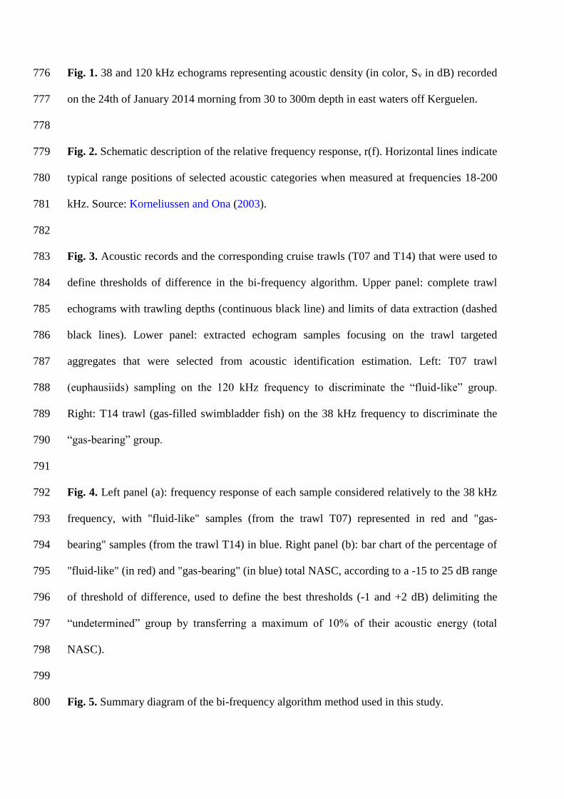
Fig. 1. 38 and 120 kHz echograms representing acoustic density (in color, Sv in dB) recorded 776
on the 24th of January 2014 morning from 30 to 300m depth in east waters off Kerguelen. 777
778
Fig. 2. Schematic description of the relative frequency response, r(f). Horizontal lines indicate 779
typical range positions of selected acoustic categories when measured at frequencies 18-200 780
kHz. Source: Korneliussen and Ona (2003). 781
782
Fig. 3. Acoustic records and the corresponding cruise trawls (T07 and T14) that were used to 783
define thresholds of difference in the bi-frequency algorithm. Upper panel: complete trawl 784
echograms with trawling depths (continuous black line) and limits of data extraction (dashed 785
black lines). Lower panel: extracted echogram samples focusing on the trawl targeted 786
aggregates that were selected from acoustic identification estimation. Left: T07 trawl 787
(euphausiids) sampling on the 120 kHz frequency to discriminate the “fluid-like” group. 788
Right: T14 trawl (gas-filled swimbladder fish) on the 38 kHz frequency to discriminate the 789
“gas-bearing” group. 790
791
Fig. 4. Left panel (a): frequency response of each sample considered relatively to the 38 kHz 792
frequency, with "fluid-like" samples (from the trawl T07) represented in red and "gas-793
bearing" samples (from the trawl T14) in blue. Right panel (b): bar chart of the percentage of 794
"fluid-like" (in red) and "gas-bearing" (in blue) total NASC, according to a -15 to 25 dB range 795
of threshold of difference, used to define the best thresholds (-1 and +2 dB) delimiting the 796
“undetermined” group by transferring a maximum of 10% of their acoustic energy (total 797
NASC). 798
799
Fig. 5. Summary diagram of the bi-frequency algorithm method used in this study. 800

801
Fig. 6. Representative diagram of the number of patches (in blue) and its derivative (in green) 802
detected along increasing Sv values from -70 to -40 dB. The value of -63 dB corresponds to a 803
threshold level over which the number of patches did not further increased. 804
805
Fig. 7. 38 and 120 kHz echograms representing acoustic density (in color, Sv in dB) recorded 806
on the 24th of January 2014 morning from 30 to 300m depth in east waters off Kerguelen for 807
(a) patches- and (b) layers structures. 808
Fig. 8. Total density (NASC, in m²·nmi-2, colored on ship track) integrated from 30 to 300 m 809
depth for each acoustic group (“gas-bearing”, fluid-like” and “undetermined” groups) and for 810
each type of structures (patches and layers). 811
812
Fig. 9. Mean vertical NASC profiles from 30 to 300 m depth of each acoustic group (“gas-813
bearing”, fluid-like” and “undetermined” groups) for day (black lines) and night (grey lines) 814
and for each type of structures (patches and layers). Dashed lines indicate the 95% confidence 815
intervals. 816


