Download - Adaptive antenna selection and Tx/Rx beamforming … Open Access Adaptive antenna selection and Tx/Rx beamforming for large-scale MIMO systems in 60 GHz channels Ke Dong1, Narayan

RESEARCH Open Access

Adaptive antenna selection and Tx/Rxbeamforming for large-scale MIMO systems in60 GHz channelsKe Dong1, Narayan Prasad2, Xiaodong Wang3* and Shihua Zhu1

Abstract

We consider a large-scale MIMO system operating in the 60 GHz band employing beamforming for high-speeddata transmission. We assume that the number of RF chains is smaller than the number of antennas, whichmotivates the use of antenna selection to exploit the beamforming gain afforded by the large-scale antenna array.However, the system constraint that at the receiver, only a linear combination of the receive antenna outputs isavailable, which together with the large dimension of the MIMO system makes it challenging to devise an efficientantenna selection algorithm. By exploiting the strong line-of-sight property of the 60 GHz channels, we propose aniterative antenna selection algorithm based on discrete stochastic approximation that can quickly lock onto a near-optimal antenna subset. Moreover, given a selected antenna subset, we propose an adaptive transmit and receivebeamforming algorithm based on the stochastic gradient method that makes use of a low-rate feedback channelto inform the transmitter about the selected beams. Simulation results show that both the proposed antennaselection and the adaptive beamforming techniques exhibit fast convergence and near-optimal performance.

Keywords: 60 GHz communication, MIMO, Antenna selection, Stochastic approximation, Gerschgorin circle, Beam-forming, Stochastic gradient

1 IntroductionThe 60 GHz millimeter wave communication hasreceived significant recent attention, and it is consideredas a promising technology for short-range broadbandwireless transmission with data rate up to multi-gigabits/s [1-4]. Wireless communications around 60 GHzpossess several advantages including huge clean unli-censed bandwidth (up to 7 GHz), compact size of trans-ceiver due to the short wavelength, and less interferencebrought by high atmospheric absorption. Standardiza-tion activities have been ongoing for 60 GHz WirelessPersonal Area Networks (WPAN) [5] (i.e., IEEE 802.15)and Wireless Local Area Networks (WLAN) [6] (i.e.,IEEE 802.11). The key physical layer characteristics ofthis system include a large-scale MIMO system (e.g., 32× 32) and the use of both transmit and receive beam-forming techniques.

To reduce the hardware complexity, typically, thenumber of radio-frequency (RF) chains employed (con-sisting of amplifiers, AD/DA converters, mixers, etc.) issmaller than the number of antenna elements, and theantenna selection technique is used to fully exploit thebeamforming gain afforded by the large-scale MIMOantennas. Although various schemes for antenna selec-tion exist in the literature [7-10], they all assume thatthe MIMO channel matrix is known or can be esti-mated. In the 60 GHz WPAN system under considera-tion, however, the receiver has no access to such achannel matrix, because the received signals are com-bined in the analog domain prior to digital basebanddue to the analog beamformer or phase shifter [11]. Butrather, it can only access the scalar output of the receivebeamformer. Hence, it becomes a challenging problemto devise an antenna selection method based on such ascalar only rather than the channel matrix. By exploitingthe strong line-of-sight property of the 60 GHz channel,we propose a low-complexity iterative antenna selectiontechnique based on the Gerschgorin circle and the

* Correspondence: [email protected] Engineering Department, Columbia University, New York, NY,10027, USAFull list of author information is available at the end of the article

Dong et al. EURASIP Journal on Wireless Communications and Networking 2011, 2011:59http://jwcn.eurasipjournals.com/content/2011/1/59

© 2011 Dong et al; licensee Springer. This is an Open Access article distributed under the terms of the Creative Commons AttributionLicense (http://creativecommons.org/licenses/by/2.0), which permits unrestricted use, distribution, and reproduction in any medium,provided the original work is properly cited.

mailto:[email protected]

http://creativecommons.org/licenses/by/2.0

stochastic approximation algorithm. Given the selectedantenna subset, we also propose a stochastic gradient-based adaptive transmit and receive beamforming algo-rithm that makes use of a low-rate feedback channel toinform the transmitter about the selected beam.The remainder of this paper is organized as follows.

The system under consideration and the problems ofantenna selection and beamformer adaptation aredescribed in Section 2. The proposed antenna selectionalgorithm is developed in Section 3. The proposedtransmit and receive adaptive beamforming algorithm ispresented in Section 4. Simulation results are providedin Section 5. Finally Section 6 concludes the paper.

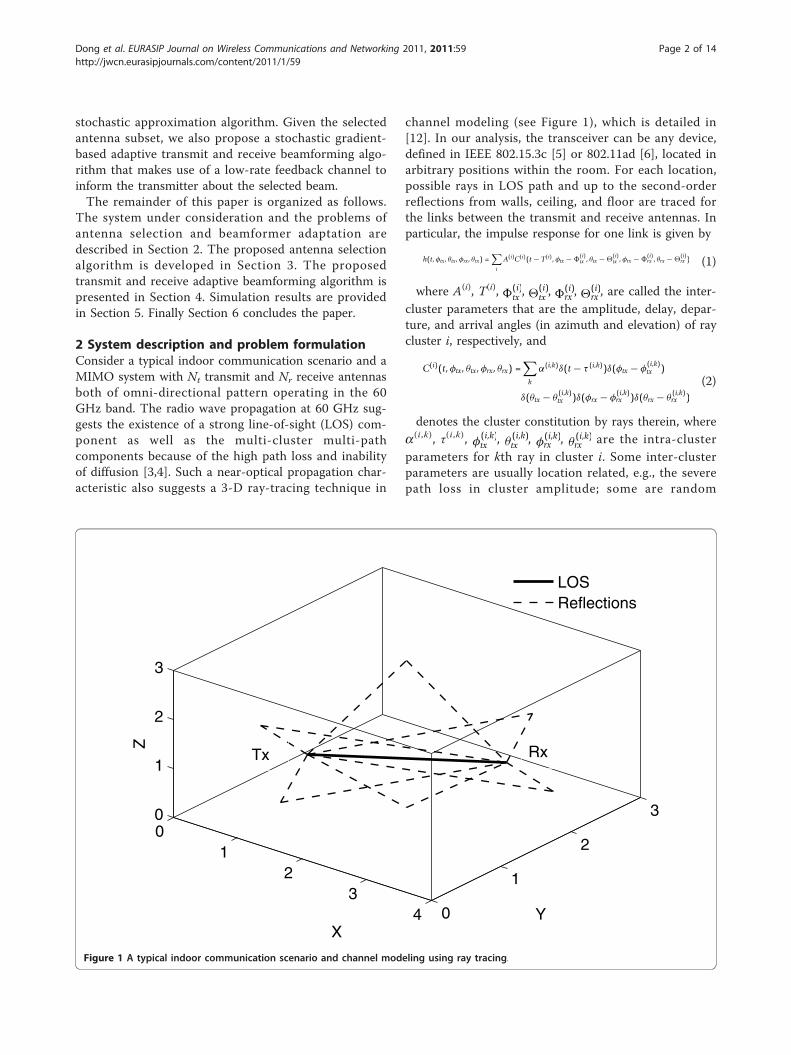
2 System description and problem formulationConsider a typical indoor communication scenario and aMIMO system with Nt transmit and Nr receive antennasboth of omni-directional pattern operating in the 60GHz band. The radio wave propagation at 60 GHz sug-gests the existence of a strong line-of-sight (LOS) com-ponent as well as the multi-cluster multi-pathcomponents because of the high path loss and inabilityof diffusion [3,4]. Such a near-optical propagation char-acteristic also suggests a 3-D ray-tracing technique in

channel modeling (see Figure 1), which is detailed in[12]. In our analysis, the transceiver can be any device,defined in IEEE 802.15.3c [5] or 802.11ad [6], located inarbitrary positions within the room. For each location,possible rays in LOS path and up to the second-orderreflections from walls, ceiling, and floor are traced forthe links between the transmit and receive antennas. Inparticular, the impulse response for one link is given by

h(t, φtx, θtx, φrx, θrx) =∑

i

A(i)C(i)(t − T(i), φtx − �(i)tx , θtx − �

(i)tx , φrx − �

(i)rx , θrx − �

(i)rx ) (1)

where A(i), T(i), �(i)tx , �

(i)tx , �

(i)rx , �

(i)rx , are called the inter-

cluster parameters that are the amplitude, delay, depar-ture, and arrival angles (in azimuth and elevation) of raycluster i, respectively, and

C(i)(t, φtx, θtx, φrx, θrx) =∑

k

α(i,k)δ(t − τ (i,k))δ(φtx − φ(i,k)tx )

δ(θtx − θ(i,k)tx )δ(φrx − φ

(i,k)rx )δ(θrx − θ

(i,k)rx )

(2)

denotes the cluster constitution by rays therein, wherea(i,k), τ(i,k), φ

(i,k)tx , θ

(i,k)tx , φ

(i,k)rx , θ

(i,k)rx are the intra-cluster

parameters for kth ray in cluster i. Some inter-clusterparameters are usually location related, e.g., the severepath loss in cluster amplitude; some are random

01

23

4 0

1

2

30

1

2

3

YX

Z

LOSReflections

RxTx

Figure 1 A typical indoor communication scenario and channel modeling using ray tracing.


Page 2 of 14

variables, e.g., reflection loss, which is typically modeledas a truncated log-normal random variable with meanand variance associated with the reflection order [12], iflinear polarization is assumed for each antenna. Besides,most intra-cluster parameters are randomly generated.On the other hand, for the short wavelength, it is rea-sonable to assume that the size of antenna array ismuch smaller than the size of the communication area,which leads to a similar geographic information for alllinks. It naturally accounts for the strong and near-deterministic LOS component and the independent rea-lizations from reflection paths in modeling the overallchannel response.In OFDM-based systems, the narrowband subchannels

are assumed to be flat fading. Thus, the equivalentchannel matrix between the transmitter and receiver isgiven by

H = [hij], with hij =Nrays∑=1

α()ij δ(t − τ0)|t=τ0

(3)

for i = 1, 2, ..., Nr and j = 1, 2, ..., Nt, where the entryhij denotes the channel response between transmitter jand receiver i by aggregating all Nrays traced raysbetween them at the delay of the LOS component, τ0;

and α()ij is the amplitude of ℓth ray in the corresponding

link. Analytically, we can further separate the channelmatrix in (3) into HLOS and HNLOS accounting for theLOS and non-LOS components, respectively

H =

√1

K + 1HNLOS +

√K

K + 1HLOS (4)

where the Rician K-factor indicates the relativestrength of the LOS component.We assume that the numbers of transmit and receive

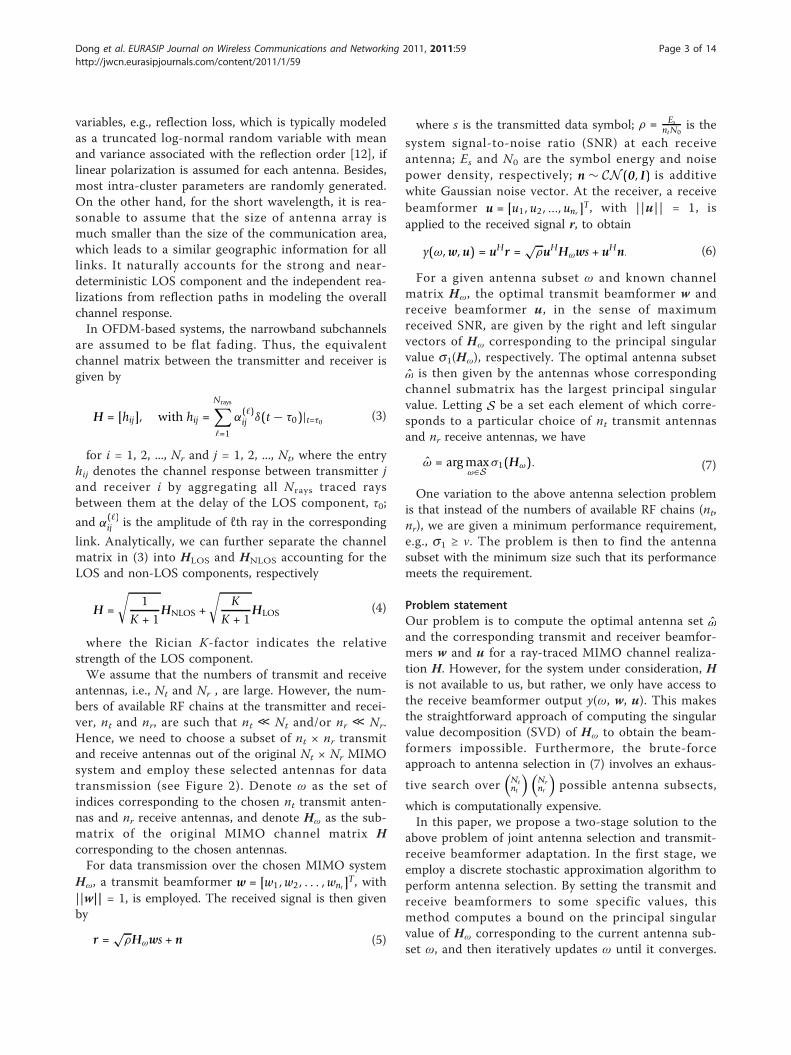
antennas, i.e., Nt and Nr , are large. However, the num-bers of available RF chains at the transmitter and recei-ver, nt and nr, are such that nt ≪ Nt and/or nr ≪ Nr.Hence, we need to choose a subset of nt × nr transmitand receive antennas out of the original Nt × Nr MIMOsystem and employ these selected antennas for datatransmission (see Figure 2). Denote ω as the set ofindices corresponding to the chosen nt transmit anten-nas and nr receive antennas, and denote Hω as the sub-matrix of the original MIMO channel matrix Hcorresponding to the chosen antennas.For data transmission over the chosen MIMO system

Hω, a transmit beamformer w = [w1, w2, . . . , wnt ]T, with

||w|| = 1, is employed. The received signal is then givenby

r =√

ρHωws + n (5)

where s is the transmitted data symbol; ρ = EsntN0

is the

system signal-to-noise ratio (SNR) at each receiveantenna; Es and N0 are the symbol energy and noisepower density, respectively; n ∼ CN (0, I) is additivewhite Gaussian noise vector. At the receiver, a receivebeamformer u = [u1, u2, ..., unr ]

T, with ||u|| = 1, isapplied to the received signal r, to obtain

y(ω, w, u) = uHr =√

ρuHHωws + uHn. (6)

For a given antenna subset ω and known channelmatrix Hω, the optimal transmit beamformer w andreceive beamformer u, in the sense of maximumreceived SNR, are given by the right and left singularvectors of Hω corresponding to the principal singularvalue s1(Hω), respectively. The optimal antenna subsetω is then given by the antennas whose correspondingchannel submatrix has the largest principal singularvalue. Letting S be a set each element of which corre-sponds to a particular choice of nt transmit antennasand nr receive antennas, we have

ω = arg maxω∈S

σ1(Hω). (7)

One variation to the above antenna selection problemis that instead of the numbers of available RF chains (nt,nr), we are given a minimum performance requirement,e.g., s1 ≥ ν. The problem is then to find the antennasubset with the minimum size such that its performancemeets the requirement.

Problem statementOur problem is to compute the optimal antenna set ω

and the corresponding transmit and receiver beamfor-mers w and u for a ray-traced MIMO channel realiza-tion H. However, for the system under consideration, His not available to us, but rather, we only have access tothe receive beamformer output y(ω, w, u). This makesthe straightforward approach of computing the singularvalue decomposition (SVD) of Hω to obtain the beam-formers impossible. Furthermore, the brute-forceapproach to antenna selection in (7) involves an exhaus-

tive search over(

Ntnt

) (Nrnr

)possible antenna subsects,

which is computationally expensive.In this paper, we propose a two-stage solution to the

above problem of joint antenna selection and transmit-receive beamformer adaptation. In the first stage, weemploy a discrete stochastic approximation algorithm toperform antenna selection. By setting the transmit andreceive beamformers to some specific values, thismethod computes a bound on the principal singularvalue of Hω corresponding to the current antenna sub-set ω, and then iteratively updates ω until it converges.


Page 3 of 14

Once the antenna subset ω is selected, in the secondstage, we iteratively update the transmit and receivebeamformers w and u using a stochastic gradient algo-rithm. At each iteration, some feedback bits are trans-mitted from the receiver to the transmitter via a low-rate feedback channel to inform the transmitter aboutthe updated transmit beamformer.In the next two sections, we discuss the detailed algo-

rithms for antenna selection and beamformer adapta-tion, respectively.

3 Antenna selection using stochasticapproximation and Gerschgorin circle3.1 The stochastic approximation algorithmAs mentioned earlier, we can only observe y(ω, w, u) in(6), which is a noisy function of the channel submatrixHω. On the other hand, the objective function to bemaximized for antenna selection is the principal singularvalue of Hω as in (7). If we could find a function j(·) ofy such that it is an unbiased estimate of s1(Hω), thenwe can rewrite the antenna selection problem (7) as

ω = arg maxω∈S

E{φ(y(ω, w, u))}. (8)

In [10], the stochastic approximation method is intro-duced to solve the problem of the form (8). The basicidea is to generate a sequence of the estimates of theoptimal antenna subset where the new estimate is basedon the previous one by moving a small step in a gooddirection towards the global optimizer. Through theiterations, the global optimizer can be found by meansof maintaining an occupation probability vector π,which indicates an estimate of the occupation

probability of one state (i.e., antenna subset). Under cer-tain conditions, such an algorithm converges to thestate that has the largest occupation probability in π.Compared with the exhaustive search approach, in thisway, more computations are performed on the “promis-ing” candidates, that is, the better candidates will beevaluated more than the others.Due to the potentially large search space in the pre-

sent problem, which not only limits the convergencespeed but also makes it difficult to maintain the occupa-tion probability vector, the algorithms in [10] canbecome inefficient. Here, we propose a modified versionof the stochastic approximation algorithm that is moreefficient to implement, and more importantly, it fitsnaturally to a procedure for estimating the principal sin-gular value of Hω based on the receive beamformer out-put y(ω, w, u) only.Specifically, we start with an initial antenna subset ω(0)

and an occupation probability vector π(0) = [ω(0), 1]T,which has only one element, with the first entry servingas the index of the antenna subset and the other entryindicating the corresponding occupation probability. Wedivide each iteration into nt + nr subiterations, and ineach sub-iteration, we replace one antenna in the cur-rent subset ω with a randomly selected antenna outsideω, resulting in a new subset w that differs from ω byone element. By comparing their corresponding objec-tive functions, the better subset is updated as well as theoccupation probability vector. This procedure isrepeated until all nt + nr antennas are updated.Instead of keeping records for all candidates, we dyna-

mically allocate and maintain record in π for the newsubset found in each iteration. If a subset already has a

RF

RF

1w1

wnt

RF

RF

u1

unr

Tx Rx

nt

1

2

Nt

1

nr

1

2

Nr

s

r

Antenna selection&

Beamforming

Antenna selection&

Beamforming

Feedback

H

Figure 2 A 60 GHz MIMO system employing antenna selection and transmit/receive beamforming.


Page 4 of 14

record in π, the corresponding occupancy probabilitywill be updated. Otherwise, a new element is appendedin π with the subset index and its occupation probabil-ity. Such a dynamic scheme avoids the huge memoryrequirement, since typically in practice, only a smallfraction of the all possible subsets is visited.We replace the selected subset with the current subset

if the current subset has a larger occupation probabil-ities in π. Otherwise, keep the selected subsetunchanged, thus completes one iteration.In general, the convergence is achieved when the

number of iterations goes to infinity. In practice, whenit happens that one subset is selected in a large number,say 100, consecutive iterations, the algorithm is regardedas convergent and terminated, and the last selected sub-set is the global (sub)optimizer. Since most of the eva-luations and decisions are generally made at thereceiver, a low-rate and error-free feedback channel isassumed to coordinate the transmitter via feedbackinformation. In each subiteration, the transmitter shouldknow in advance which transmit antennas have beenleft in the current subset (i.e., ω(n)) from last subitera-tion (because the current subset might have been chan-ged in the previous subiteration), and then couldgenerate a new subset by replacing the one with a ran-dom transmit antenna outside ω(n). Without feedbackan invalid situation might happen such that a transmitantenna, which is already assigned to one RF chain inthe current subset, is selected again for another RFchain. In other words, feedback is necessary only in sub-iterations in which the current subset has changed forthe transmit antennas during the last update in the pre-vious subiteration. This implies that the amount of feed-backs is rather limited.The modified stochastic approximation algorithm for

antenna selection is summarized in Algorithm 1. Inwhat follows we discuss the form of the objective func-tion j(·) in (8) and its calculation.

3.2 Estimating the principal singular value usingGerschgorin circleThe Gerschgorin circle theorem [13] gives a range on acomplex plane within which all the eigenvalues of asquare matrix lie. In this section, we show that a goodapproximation to the largest eigenvalue can be calcu-lated as long as the Rician K-factor is high enough. Bycalculating the G-circles, a simple estimator j(·) of theobjective function in (8) is developed and employed inthe stochastic approximation algorithm for antennaselection, i.e., Algorithm 1.Denote the channel submatrix of the selected antenna

subset by Hω = [h1, h2, . . . , hnt ], where hk ∈ Cnr×1 is theSIMO channel between the kth transmit antenna andthe nr receive antennas in the subset ω. The correlation

matrix of Hω is then

Rω = HHω Hω =

⎡⎢⎢⎢⎣

hH1 h1 hH

1 h2 · · · hH1 hnt

hH2 h1 hH

2 h2 · · · hH2 hnt

......

. . ....

hHnt

h1 hHnt

h2 · · · hHnt

hnt

⎤⎥⎥⎥⎦ . (9)

Denote the eigenvalues of Rω in descending order asλ1 ≥ λ2 ≥ · · · ≥ λnt. Then, according to the Gerschgorincircles theorem [13], these nt eigenvalues lie in at leastone of the following circles

{λ : |λ − hHk hk| ≤ ρk}, k = 1, . . . , nt , (10)

with the radius of the kth circle being

ρk =nt∑

=1,�=k

|hHk h|, k = 1, . . . , nt . (11)

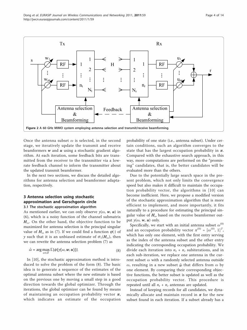
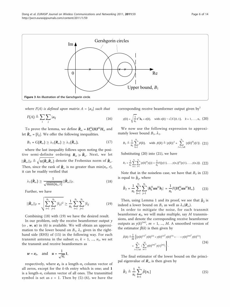
The above nt circles are centered along the positivereal axis. Since the correlation matrix Rω is positivesemi-definite, all eigenvalues are located along the posi-tive real axis within these circles, as illustrated in Figure3. Note that from (10) to (11), a circle with a larger cen-ter coordinate implies a larger channel gain for the cor-responding transmit antenna; and a circle with a smallerradius implies a smaller channel correlation between thecorresponding antenna and the other selected antennas.As seen from Figure 3, the right-most point among thent circles is the upper bound for all eigenvalues andsuch a point can be used as the estimate of the largesteigenvalue of Rω. That is,

λ1 ≤ maxk=1,...,nt

{||hk||2 +nt∑

=1,�=k

|hHk h|} � B1. (12)

Since the principal singular value s1 of Hω is relatedto l1 through λ1 = σ 2

1 , we can rewrite (7) as

ω = arg maxω∈S

λ1(Rω). (13)

Note that, B1 is the maximum over the l1 norms ofthe rows of Rω. In particular, letting Rω = [rij] we have

B1 = G(Rω) � maxi

⎧⎨⎩

nt∑j=1

|rij|⎫⎬⎭ (14)

Next we prove a lemma that provides a useful boundon B1 and l1.Lemma 1 For any semi-unitary matrix U ∈ Cnr×rsuch

that UHU = I, we have

B1 ≥ λ1(Rω) ≥ 1

nt√

min{nt , r}F(HHω UUHHω) (15)


Page 5 of 14

where F(A) is defined upon matrix A = [aij] such that

F(A) �∑

i

∑j

|aij| (16)

To prove the lemma, we define Rω = HHω UUHHω and

let Rω = [rij]. We offer the following inequalities.

B1 = G(Rω) ≥ λ1(Rω) ≥ λ1(Rω), (17)

where the last inequality follows upon noting the posi-tive semi-definite ordering Rω � Rω. Next, we let

||Rω||F �√

tr(RωRω) denote the Frobenius norm of Rω.

Then, since the rank of Rω is no greater than min{nt, r},it can be readily verified that

λ1(Rω) ≥ 1√min{nt , r} ||Rω||F . (18)

Further, we have

||Rω||F =

√√√√ nt∑i=1

nt∑j=1

|rij|2 ≥ 1nt

nt∑i=1

nt∑j=1

|rij| (19)

Combining (18) with (19) we have the desired result.In our problem, only the receive beamformer output y

(ω , w, u) in (6) is available. We will obtain an approxi-mation to the lower bound on B1, l1 given in the right-hand side (RHS) of (15) in the following way. For eachtransmit antenna in the subset ω, k = 1, ..., nt, we setthe transmit and receive beamformers as

w = ek, and u =1√nr

1,

respectively, where ek is a length-nt column vector ofall zeros, except for the k-th entry which is one; and 1is a length-nr column vector of all ones. The transmittedsymbol is set as s = 1. Then by (5)-(6), we have the

corresponding receive beamformer output given by1

y(k) =

√1nr

1Thk + v(k), with v(k) ∼ CN (0, 1), k = 1, . . . , nt . (20)

We now use the following expression to approxi-mately lower bound B1, l1.

B2 � 1nt

nt∑k=1

β(k), with β(k) � |y(k)|2 +nt∑

=1,�=k

|y(k)Hy()|. (21)

Substituting (20) into (21), we have

B2 =1nt

nt∑k=1

nt∑j=1

|y(k)Hy(j)| =1nt

F([y(1), . . . , y(nt)]H[y(1), . . . , y(nt)]). (22)

Note that in the noiseless case, we have that B2 in (22)is equal to B2, where

B2 =1nt

nt∑k=1

nt∑j=1

|hHk uuHhj| =

1nt

F(HHω uuHHω). (23)

Then, using Lemma 1 and its proof, we see that B2 isindeed a lower bound on B1 as well as l1(Rω).In order to mitigate the noise, for each transmit

beamformer ek, we will make multiple, say M transmis-sions, and denote the corresponding receive beamformeroutputs as y(k)(m), m = 1, ..., M. A smoothed version ofthe estimator b(k) is then given by

β(k) � 1M

{[y(k)(1)H

y(k)(2) + y(k)(2)H

y(k)(3) + · · · + y(k)(M)H

y(k)(1)]

+nt∑

=1,�=k

|M∑

m=1

y(k)(m)H

y()(m)|⎫⎬⎭ .

(24)

The final estimator of the lower bound on the princi-pal eigenvalue of Rω is then given by

B2 � 1nt

nt∑k=1

β(nt) (25)

Im

Re

Gershgorin circles

Upper bound, B1

0

Figure 3 An illustration of the Gerschgorin circle.


Page 6 of 14

It is easily seen that both the 1st-order and 2nd-ordernoise terms are averaged out in B2, so that as M ® ∞we have

B2 → B2. (26)

Recall that in the stochastic approximation algorithmfor antenna selection, at each iteration, we sequentiallyupdate the transmit and receive antennas and computethe corresponding objective functions. The aboveapproach for calculating the objective function fits natu-rally in this framework, since for each transmit antennacandidate, we only need to transmit a pilot signal fromit and then compute the corresponding β(k). The com-plete antenna selection algorithm is now summarized inAlgorithm 1.Remark-1: We note that a typical scenario in 60

GHz has a strongly LOS channel with K ≫ 1 and onedominant path, so that HLOS = abH is a rank onematrix. Moreover, in many applications, it is feasibleto retain all receive antenna elements, so that the taskreduces to selection of the optimal transmit antennasubset. In this case, neglecting HNLOS and the back-ground noise (which holds for K, M ≫ 1), it can beverified that the transmit antenna subset which maxi-mizes B2also results in the largest eigenvalue. In parti-cular

ω = arg maxω∈S

λ1(Rω) ≈ arg maxω∈S

B2(ω). (27)

where we use B2(ω)to denote the B2evaluated for aparticular subset and where the approximation becomesexact in the limit of large K, M.Remark-2: So far, we have assumed that only one

receive beamformer u = 1√nr

1 is employed for a given

choice of receive antenna subset. Suppose upto r receivebeamformers {u1, ..., ur} (which are columns of a nr × nrunitary matrix) could be used for each transmit beam-former ek, k = 1, ..., nt. Then, invoking Lemma 1 anddefiningy(v, uj) = [y(ω, e1, uj), . . . , y(ω, ent , uj)], j = 1, ..., r, wesee that a better approximation can be obtained as

1

nt√

min{r, nt}F

⎛⎝ r∑

j=1

y(ω, uj)Hy(ω, uj)

⎞⎠ , (28)

or its smoother version

1

nt√

min{r, nt}nt∑

k=1

γ (k) (29)

where

γ (k) � 1M

⎧⎨⎩

r∑j=1

[y(ω, ek, uj)(1)H

y(ω, ek, uj)(2) + · · · + y(ω, ek, uj)

(M)H

y(ω, ek, uj)(1)]

+nt∑

=1,�=k

|r∑

j=1

M∑m=1

y(ω, ek, uj)(m)H

y(ω, e, uj)(m)|

⎫⎬⎭ .

(30)

Finally, we note that for a given nt, nr, r, the channel-independent constant can be omitted when computingthe metric in (25) or (30).

4 Adaptive Tx/Rx beamforming with low-ratefeedbackOnce the antenna subset Hω is chosen, the transmit andreceive beamformers w and u will be computed. Asmentioned in Section 2, w and u should be chosen tomaximize the received SNR, or alternatively, to maxi-mize the power of the receive beamformer output in (6),|y(ω, w, u)|2, i.e.,

(w, u) = arg maxw∈Cnt , ‖w‖=1; u∈Cnr ,‖u‖=1

|y(v, w, u)|2. (31)

Since the channel matrix Hω is not available, we resortto a simple stochastic gradient method for updating thebeamformers.

4.1 Stochastic gradient algorithm for beamformer updateThe algorithm for the beamformer update is a generali-zation of [14] and is described as follows. At each itera-tion, given the current beamformers (w, u), we generateKt perturbation vectors for the transmit beamformer,pj ∼ CN (0, I), j = 1, ..., Kt, and Kr perturbation vectorsfor the receive beamformer, qi ∼ CN (0, I), i = 1, ..., Kr.Then for each of the normalized perturbed transmit-receive beamformer pairs(

w + βpj

||w + βpj||,

u + βqi

||u + βqi||

), (32)

Algorithm 1 Adaptive antenna selection using sto-chastic approximation and G-circleINITIALIZATION:

n ⇐ 0;Select initial antenna subset ω(0) and set π(0) = [ω(0),1]T;Transmit pilot signals from each selected transmitantenna and obtain the received signals using theselected receive antennas {y(k)(m), m = 1, ..., M; k =1, ..., nt + nr};Compute the objective function j(ω(0)) using (24)-(25);


Page 7 of 14

Set selected antenna subset ω = ω(0).For n = 1, 2, ...

For k = 1, 2, ..., nt + nr

SAMPLING AND EVALUATION:

Replace the kth element in ω(n) by a randomlyselected antenna that is not in ω(n) to obtain a newsubset ω(n) that differs with ω(n) by only oneelement;For a newly selected transmit antenna, transmit pilotsignals from it and obtain the received signals {y(k)(m), m = 1, ..., M};For a newly selected receive antenna, sequentiallytransmit pilot signals from all transmit antennas andobtain the received signals;Recalculate the objective function φ(ω(n)) using (24)-(25).

ACCEPTANCE:

If φ(ω(n)) > φ(ω(n)) ThenUpdate ω(n) = ω(n);If ω(n) is NOT recorded in π Then

Append the column [ω(n), 0]T to π ;EndIfFeed back ω(n) if the update affects any transmitantenna therein

EndIf

ADAPTIVE FILTERING:

Set forgetting factor: μ(n) = 1/n;π(n) = [1 - μ(n + 1)] π (n);π(n)(ω(n)) = π(n)(ω(n)) + μ(n + 1);

EndFor (k)

SELECTION:

If π (n)(ω(n)) > π (n)(ω) ThenSet ω = ω(n);

EndIfω(n+1) = ω(n); π(n+1) = π (n);

EndFor (n)

where b is a step-size parameter, the correspondingreceived output power |y|2 are measured, and the effec-tive channel gain |uHHωw|

2 can be used as a perfor-mance metric independent of transmit power. Finally,the beamformers are updated using the perturbationvector pair that gives the largest output power at thereceiver. The transmitter is informed about the selectedperturbation vector by a ⌈log Kt⌉-bit message from the

receiver. The algorithm is regarded as convergent, andthe iteration terminates when the performance metricfluctuates below a tolerance threshold. The algorithm issummarized as follows.Algorithm 2 Stochastic gradient algorithm for beam-

former update

INITIALIZATION:Initialize w(0) and u(0)

For n = 0, 1, ...PROBING:

Generate Kt and Kr new beamformer vectorsusing (32) based on w (n) and u(n),respectively;Evaluate the received power |y|2 for each oneof the KtKr perturbed beamformer pairs;

UPDATE AND FEEDBACK:Let pj* and qi* be the perturbation vectorsthat give the largest received power;Feedback the index of the best transmit per-turbation vector using ⌈log Kt⌉ bits;Update the beamformers:

w(n+1) = (w(n) + βpj∗)/||w(n) + βpj∗ ||, u(n+1) = (u(n) + βqi∗ )/||u(n) + βqi∗ ||.

EndFor

4.2 Implementation issuesWe next discuss some implementation issues related tothe above stochastic gradient algorithm for beamformerupdate.InitializationA good initialization can considerably speed up theconvergence of the above stochastic gradient algorithmcompared with random initialization. For the applica-tion considered in this paper, recall that the channelconsists of a deterministic LOS component HLOS and arandom component. When the K-factor is high, theLOS component mostly determines the largest singularmode. Hence, we can initialize the transmit andreceive beamformers as the right and left singular vec-tors of HLOS, respectively, which we will call it a hotstart.ParameterizationSince both w and u have unit norms, we can representthem using spherical coordinates. Considerw = [w1, w2, . . . , wnt ]

T as an example. Expanding v = [Re{wT}, Im{wT}]T, it is equivalent to a point on the surfaceof the 2nt-dimensional unit sphere. Thus, v can be para-meterized by (2nt - 1)-dimensional vector ψ as follows[15]


Page 8 of 14

v1 = cos ψ1, (33)

v2 = sin ψ1 cos ψ2, (34)

... (35)

v2nt−1 = sin ψ1 sin ψ2 · · · sin ψ2nt−2 cos ψ2nt−1, (36)

v2nt = sin ψ1 sin ψ2 · · · sin ψ2nt−2 sin ψ2nt−1, (37)

with 0 < ψi < π , 1 ≤ i ≤ 2nt − 2; and 0 < ψ2nt−1 ≤ 2π . (38)

Given the vector v or equivalently ψ, to obtain a newperturbed weight vector near v, we can set an arbitrarysmall ε > 0 and generate i.i.d. random variables {δi}2nt−2

i=1 ,which are uniformly distributed within [− ε

2 , ε2 ] and

another independent uniform random variableδ2nt−1 ∈ [−ε, ε]. Then, new parameters are obtainedwithin some predefined boundaries, given by

ψ i = [ψi + δi]biai

, 1 ≤ i ≤ 2nt − 1, (39)

where [x]ba denotes that x is confined in the interval of

[a, b], i.e., [x]ba = x if a ≤ x ≤ b, [x]b

a = b if x > b and

[x]ba = a if x < a. As a result, uniform search for the bet-

ter weight vector is confined within a fixed spacedefined by [ai, bi], 1 ≤ i ≤ 2nt - 1 and the range of theperturbation depends on the definition of {δi}. Forexample, given a hot start, the current weight vectormaybe very close to the optimizer, and it is necessary toset a smaller search region and a finer perturbation.Parallel receptionSince at each iteration, the best beamformer pair is cho-sen out of KtKr combinations based on the correspond-ing output powers |y|2, it would require KtKr

transmissions. In practice, instead of switching to differ-ent the receive beamformers and making the corre-sponding transmissions for each transmit beamformer,we can set up Kr parallel receiver beamformers to obtainKr receiver outputs simultaneously. Then, only Kt trans-missions are needed for each iteration.Conservative updateIf all candidate Kt + Kr beamformers at each iterationare generated anew, then the algorithm is termedaggressive. On the other hand, a conservative strategykeeps the best transmit and receive beamformers fromthe previous iteration and generates Kt -1 new transmi-tand Kr -1 new receive beamformers for the currentiteration. With a fixed step size and a single feedbackbit, the advantage of the aggressive update is the quickerconvergence. But with multiple feedback bits, such anadvantage is less significant. Therefore, the conservative

update is preferable for a finer performance uponconvergence.

5 Simulation resultsWe consider an empty conference room with dimension4m(L) × 3m(W) × 3m(H) for analysis, in which a large-scale MIMO system with Nt = 32 and Nr = 10 transmitand receive antennas operating at the 60 GHz band israndomly located. All the antennas are omni-directionalwith 20 dBi gain and vertical linear polarized. There are10 available RF chains at both the transmitter and thereceiver, i.e., nt = 10 and nr = 10. To generate the chan-nel realizations, 3-D ray tracing is performed betweenthe transceiver using the inter- and intra-cluster para-meters specified for the conference room scenario in[12]. By the result of ray tracing, the 32 × 10 channelmatrix is gathered using (3). The channel remains staticduring antenna selection and beamformer update. Notethat the channels simulated in the sequel are covered byRemark-1 in Section 3.2. Also, OFDM-based PHY isused as suggested in [5], where 512 subchannels dividetotal 2.16 GHz bandwidth. The default system SNR isassumed as r = 60dB. The insertion loss on signalpower due to the switches between the RF chains andantennas is considered as an extra 5 dB increase innoise figure.

Performance of antenna selection with fixed sizeThe performance of Algorithm 1 for antenna selection ina single run is shown in Figure 4. Both the G-circle esti-mates B2 given by (24)-(25) as well as the actual largesteigenvalues of the selected antenna subsets are plottedfor the first 200 iterations as a zoom-in view. The num-ber of transmissions for obtaining the smoothed estimatein (24) is M = 20. Since the search space is quite large, i.e., (32

10 ) = 64512240, in the same figure, we also plot thelargest eigenvalues of the best and the worst subsetsamong 1,000 randomly selected antenna subsets. More-over, the single-run performance of the antenna selectionalgorithm in [10] is also shown. In Figure 5, the averageperformance of 100 runs for the above schemes is plottedin a larger span of iterations. Several observations are inorder. First, it is seen that the G-circle estimates are quiteclose to the actual largest eigenvalues, which validates theuse of G-circle as a metric for antenna selection in strongline-of-sight channels. Secondly, Algorithm 1 has a muchfaster convergence rate than the algorithm in [10], whichat each iteration picks the next candidate subset ran-domly and independent of the current subset, whereasAlgorithm 1 searches for the next candidate subset in theneighborhood of the current subset. Thirdly, Algorithm 1can lock onto a near-optimal antenna subset very quickly,e.g., in 10-20 iterations, and it significantly outperforms


Page 9 of 14

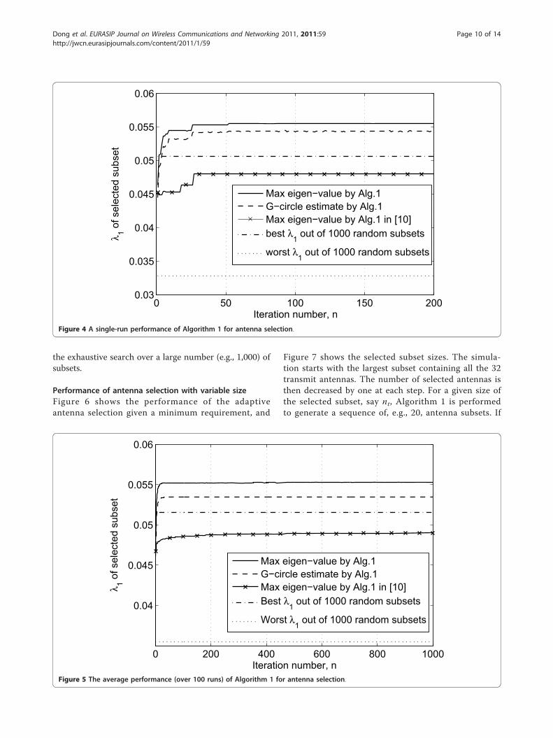
the exhaustive search over a large number (e.g., 1,000) ofsubsets.

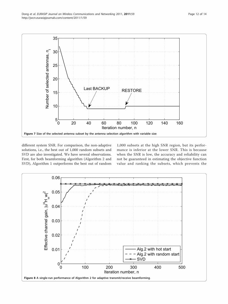
Performance of antenna selection with variable sizeFigure 6 shows the performance of the adaptiveantenna selection given a minimum requirement, and

Figure 7 shows the selected subset sizes. The simula-tion starts with the largest subset containing all the 32transmit antennas. The number of selected antennas isthen decreased by one at each step. For a given size ofthe selected subset, say nt, Algorithm 1 is performedto generate a sequence of, e.g., 20, antenna subsets. If

0 50 100 150 2000.03

0.035

0.04

0.045

0.05

0.055

0.06

Iteration number, n

λ 1 of s

elec

ted

subs

et

Max eigen−value by Alg.1G−circle estimate by Alg.1Max eigen−value by Alg.1 in [10]best λ

1 out of 1000 random subsets

worst λ1 out of 1000 random subsets

Figure 4 A single-run performance of Algorithm 1 for antenna selection.

0 200 400 600 800 1000

0.04

0.045

0.05

0.055

0.06

Iteration number, n

λ 1 of s

elec

ted

subs

et

Max eigen−value by Alg.1G−circle estimate by Alg.1Max eigen−value by Alg.1 in [10]Best λ

1 out of 1000 random subsets

Worst λ1 out of 1000 random subsets

Figure 5 The average performance (over 100 runs) of Algorithm 1 for antenna selection.


Page 10 of 14

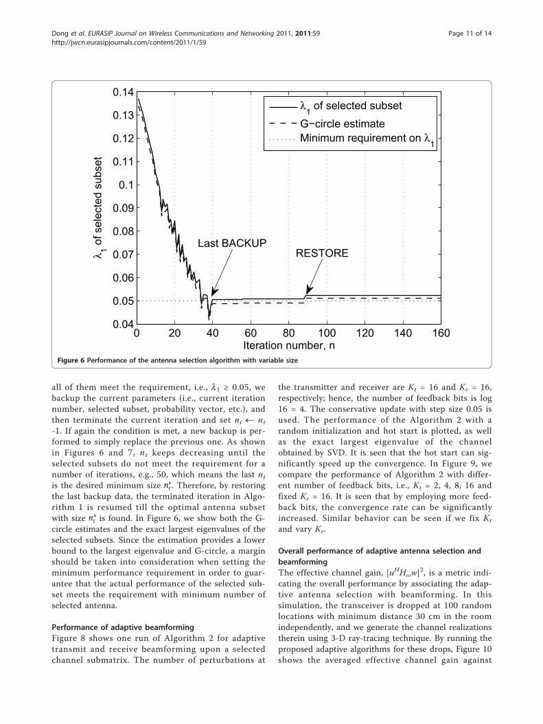
all of them meet the requirement, i.e., l1 ≥ 0.05, webackup the current parameters (i.e., current iterationnumber, selected subset, probability vector, etc.), andthen terminate the current iteration and set nt ¬ nt-1. If again the condition is met, a new backup is per-formed to simply replace the previous one. As shownin Figures 6 and 7, nt keeps decreasing until theselected subsets do not meet the requirement for anumber of iterations, e.g., 50, which means the last ntis the desired minimum size n∗

t . Therefore, by restoringthe last backup data, the terminated iteration in Algo-rithm 1 is resumed till the optimal antenna subsetwith size n∗

t is found. In Figure 6, we show both the G-circle estimates and the exact largest eigenvalues of theselected subsets. Since the estimation provides a lowerbound to the largest eigenvalue and G-circle, a marginshould be taken into consideration when setting theminimum performance requirement in order to guar-antee that the actual performance of the selected sub-set meets the requirement with minimum number ofselected antenna.

Performance of adaptive beamformingFigure 8 shows one run of Algorithm 2 for adaptivetransmit and receive beamforming upon a selectedchannel submatrix. The number of perturbations at

the transmitter and receiver are Kt = 16 and Kr = 16,respectively; hence, the number of feedback bits is log16 = 4. The conservative update with step size 0.05 isused. The performance of the Algorithm 2 with arandom initialization and hot start is plotted, as wellas the exact largest eigenvalue of the channelobtained by SVD. It is seen that the hot start can sig-nificantly speed up the convergence. In Figure 9, wecompare the performance of Algorithm 2 with differ-ent number of feedback bits, i.e., Kt = 2, 4, 8, 16 andfixed Kr = 16. It is seen that by employing more feed-back bits, the convergence rate can be significantlyincreased. Similar behavior can be seen if we fix Kt

and vary Kr.

Overall performance of adaptive antenna selection andbeamformingThe effective channel gain, |uHHωw|

2, is a metric indi-cating the overall performance by associating the adap-tive antenna selection with beamforming. In thissimulation, the transceiver is dropped at 100 randomlocations with minimum distance 30 cm in the roomindependently, and we generate the channel realizationstherein using 3-D ray-tracing technique. By running theproposed adaptive algorithms for these drops, Figure 10shows the averaged effective channel gain against

0 20 40 60 80 100 120 140 1600.04

0.05

0.06

0.07

0.08

0.09

0.1

0.11

0.12

0.13

0.14

Iteration number, n

λ 1 of s

elec

ted

subs

etλ

1 of selected subset

G−circle estimateMinimum requirement on λ

1

RESTORELast BACKUP

Figure 6 Performance of the antenna selection algorithm with variable size.


Page 11 of 14

different system SNR. For comparison, the non-adaptivesolutions, i.e., the best out of 1,000 random subsets andSVD are also investigated. We have several observations.First, for both beamforming algorithm (Algorithm 2 andSVD), Algorithm 1 outperforms the best out of random

1,000 subsets at the high SNR region, but its perfor-mance is inferior at the lower SNR. This is becausewhen the SNR is low, the accuracy and reliability cannot be guaranteed in estimating the objective functionvalue and ranking the subsets, which prevents the

0 20 40 60 80 100 120 140 1605

10

15

20

25

30

35

Iteration number, n

Num

ber o

f sel

ecte

d an

tenn

as, n

t

Last BACKUP RESTORE

Figure 7 Size of the selected antenna subset by the antenna selection algorithm with variable size.

0 100 200 300 400 5000

0.01

0.02

0.03

0.04

0.05

0.06

Iteration number, n

Effe

ctiv

e ch

anne

l gai

n, |u

HH

ωw

|2

Alg.2 with hot startAlg.2 with random startSVD

Figure 8 A single-run performance of Algorithm 2 for adaptive transmit/receive beamforming.


Page 12 of 14

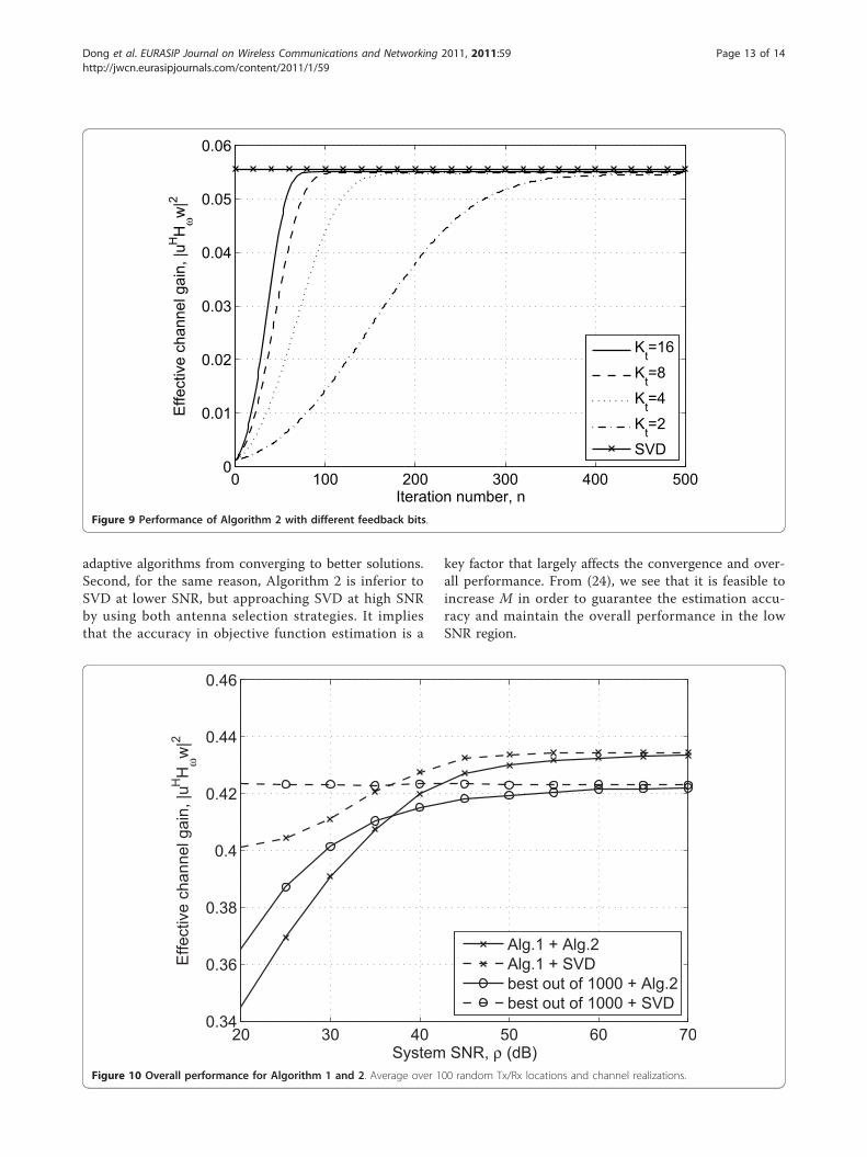
adaptive algorithms from converging to better solutions.Second, for the same reason, Algorithm 2 is inferior toSVD at lower SNR, but approaching SVD at high SNRby using both antenna selection strategies. It impliesthat the accuracy in objective function estimation is a

key factor that largely affects the convergence and over-all performance. From (24), we see that it is feasible toincrease M in order to guarantee the estimation accu-racy and maintain the overall performance in the lowSNR region.

0 100 200 300 400 5000

0.01

0.02

0.03

0.04

0.05

0.06

Iteration number, n

Effe

ctiv

e ch

anne

l gai

n, |u

HH

ωw

|2

Kt=16

Kt=8

Kt=4

Kt=2

SVD

Figure 9 Performance of Algorithm 2 with different feedback bits.

20 30 40 50 60 700.34

0.36

0.38

0.4

0.42

0.44

0.46

System SNR, ρ (dB)

Effe

ctiv

e ch

anne

l gai

n, |u

HH

ωw

|2

Alg.1 + Alg.2Alg.1 + SVDbest out of 1000 + Alg.2best out of 1000 + SVD

Figure 10 Overall performance for Algorithm 1 and 2. Average over 100 random Tx/Rx locations and channel realizations.


Page 13 of 14

6 ConclusionsWe have proposed a sequential antenna selection algo-rithm and an adaptive transmit/receive beamformingalgorithm for large-scale MIMO systems in the 60 GHzband. One constraint of the system under considerationis that the receiver can only access a linear combinationof the receive antenna outputs, which makes the tradi-tional antenna selection schemes based on the channelmatrix not applicable. The proposed antenna selectionmethod uses a bound on the largest singular value of thechannel matrix based on the Gerschgorin circle. Themethod is particularly useful over the 60 GHz channel,which has a strong line-of-sight component, and itemploys a discrete stochastic approximation technique toquickly lock onto a near-optimal antenna subset. Wehave also proposed an adaptive joint transmit and receivebeamforming technique based on the stochastic gradientmethod that makes use of a low-rate feedback channel toinform the transmitter about the selected beam. Simula-tion results show that both the proposed antenna selec-tion and the adaptive beamforming techniques exhibitfast convergence and near-optimal performance.

Note1Note that in obtaining (20) without loss of generalitywe have absorbed r into H.

AcknowledgementsThe authors wish to acknowledge financial support from the National KeySpecialized Project of China (2009ZX03003-008-02) and the National ScienceFoundation of China (60902043).

Author details1Xi’an Jiao Tong University, Xi’an, China 2NEC Labs America, Princeton, NJ,08540, USA 3Electrical Engineering Department, Columbia University, NewYork, NY, 10027, USA

Competing interestsThe authors declare that they have no competing interests.

Received: 24 November 2010 Accepted: 11 August 2011Published: 11 August 2011

References1. CH Doan, S Emami, DA Sobel, AM Niknejad, RW Brodersen, Design considerations

for 60 GHz CMOS radios. IEEE Commun Mag. 42(12), 132–140 (2004)2. SK Yong, CC Chong, An overview of multigigabit wireless through

millimeter wave technology: potentials and technical challenges. EURASIP JWirel Commun Netw. 2007(1), 50–50 (2007)

3. A Seyedi, On the capacity of wideband 60 GHz channels with antennadirectionality, in IEEE GLOBECOM 2007 (Washington D.C., 2007), pp. 4532–4536

4. J Nsenga, W Van Thillo, F Horlin, A Bourdoux, R Lauwereins, Comparison ofOQPSK and CPM for communications at 60 GHz with a nonideal front end.EURASIP J Wirel Commun Netw. 2007(1), 51–51 (2007)

5. IEEE Standard for Information technology - Telecommunications andinformation exchange between systems - Local and metropolitan areanetworks - Specific requirements. Part 15.3: Wireless Medium Access Control(MAC) and Physical Layer (PHY) Specifications for High Rate WirelessPersonal Area Networks (WPANs) Amendment 2: Millimeter-wave-basedAlternative Physical Layer Extension, IEEE Std 802.15.3c-2009 (Amendment toIEEE Std 802.15.3-2003) (2009)

6. Draft standard for IEEE 802.11ad, IEEE P802.11ad/D0.1, June 20107. M Gharavi-Alkhansari, AB Gershman, Fast antenna subset selection in MIMO

systems. IEEE Trans Sig Proc. 52(2), 339–347 (2004). doi:10.1109/TSP.2003.821099

8. A Gorokhov, D Gore, A Paulraj, Receive antenna selection for MIMO flat-fading channels: Theory and algorithms. IEEE Trans Inform Theory 49(10),2687–2696 (2003). doi:10.1109/TIT.2003.817458

9. AF Molisch, MZ Win, YS Choi, JH Winters, Capacity of MIMO systems withantenna selection. IEEE Trans Wirel Commun. 4(4), 1759–1772 (2005)

10. I Berenguer, X Wang, V Krishnamurthy, Adaptive MIMO antenna selection viadiscrete stochastic optimization. IEEE Trans Sig Proc. 53(11), 4315–4329 (2005)

11. C Choi, E Grass, R Kraemer, T Derham, S Roblot, L Cariou, P Christin,Beamforming training for ieee 802.11ad. doc.: IEEE 802.11-10/0493r1.(May 2010)

12. A Maltsev, Channel models for 60 GHz WLAN systems. doc.: IEEE 802.11-09/0334r8. (2010)

13. R Horn, C Johnson, Matrix Analysis (Cambridge University Press, New York,NY, 1985)

14. BC Banister, JR Zeidler, A simple gradient sign algorithm for transmitantenna weight adaptation with feedback. IEEE Trans Sig Proc. 51(5),1156–1171 (2003). doi:10.1109/TSP.2002.808104

15. X Wang, V Krishnamurthy, J Wang, Stochastic gradient algorithms fordesign of minimum error-rate linear dispersion codes in MIMO wirelesssystems. IEEE Trans Sig Proc. 54(4), 1242–1255 (2006)

doi:10.1186/1687-1499-2011-59Cite this article as: Dong et al.: Adaptive antenna selection and Tx/Rxbeamforming for large-scale MIMO systems in 60 GHz channels.EURASIP Journal on Wireless Communications and Networking 2011 2011:59.

Submit your manuscript to a journal and benefi t from:

7 Convenient online submission

7 Rigorous peer review

7 Immediate publication on acceptance

7 Open access: articles freely available online

7 High visibility within the fi eld

7 Retaining the copyright to your article

Submit your next manuscript at 7 springeropen.com


Page 14 of 14

http://www.springeropen.com/

http://www.springeropen.com/