

Adaptive Runge-Kutta
• addresses the problem of functions that change rapidly at a point
0
1
2
3
4
5
6
0 5 10 15 20 25 30
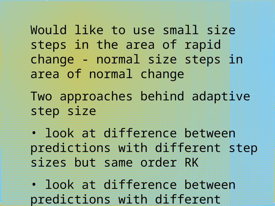
Would like to use small size steps in the area of rapid change - normal size steps in area of normal change
Two approaches behind adaptive step size
• look at difference between predictions with different step sizes but same order RK
• look at difference between predictions with different order RK

Step-halving or adpartive Runge-Kutta
let y1 be single-step prediction
let y2 be prediction using two half steps
12 yy
The correction is
1522
yy
fifth order accurate
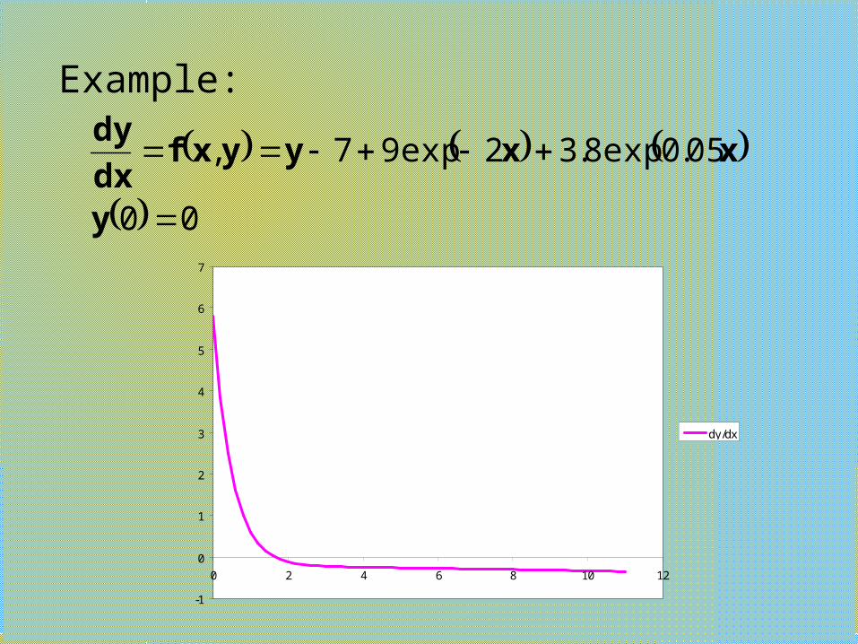
Example:
00
05.0exp8.32exp97,
y
xxyyxfdx
dy
-1
0
1
2
3
4
5
6
7
0 2 4 6 8 10 12
dy/dx

Integrate y’ from x=0 to 2 using h=2, and improve using adaptive RK
Complete step results areh 2x RK k1 k2 k3 k40 0 5.8 0.60176 0.6018 -0.11112 2.69863 -0.1111 -0.2175 -0.2175 -0.2423
Half step results areh 1x RK k1 k2 k3 k40 0 5.8 2.00221 2.0022 0.60181 2.40177 0.60176 0.08315 0.0831 -0.11112 2.53897 -0.1111 -0.1862 -0.1862 -0.2175

The correction is
01064.015
69863.253897.215
22 step onesteps two
yyEa
The corrected value is 528324.201064.0538969.2
Compare to true value y(2)=2.524369
%2.0
%6.0
%9.6
1
2
acorr
a
a
E
E
E
Runge-Kutta-Fehlberg
Uses two different RK predictions of different order
Special choice of methods lets you use results from 4th order in 5th order RK - then combine them

Fourth order RK
hkkkkyy ii
64311 1771
512
594
125
621
250
378
37
Fifth order RK
hkkkkkyy ii
654311 4
1
14336
277
55296
13525
48384
18575
27648
2825

Formula for k’s
hkhkhkhkhkyhxfk
hkhkhkhkyhxfk
hkhkhkyhxfk
hkhkyhxfk
hkyhxfk
yxfk
ii
ii
ii
ii
ii
ii
543216
43215
3214
213
12
1
4096
253
110592
44275
13824
575
512
175
55296
1631,
8
7
27
35
27
70
2
5
54
11,
5
6
10
9
10
3,
5
3
40
9
40
3,
10
3
5
1,
5
1
,

00
05.0exp8.32exp97,
y
xxyyxfdx
dy
Example
Use h=2, and the RKF method
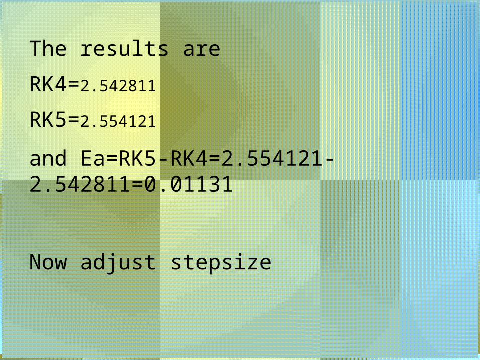
The results are
RK4=2.542811
RK5=2.554121
and Ea=RK5-RK4=2.554121-2.542811=0.01131
Now adjust stepsize

If Ea is too small, increase step size
If Ea is too large, decrease step size
presentoldnew
dx
dyhy
hh
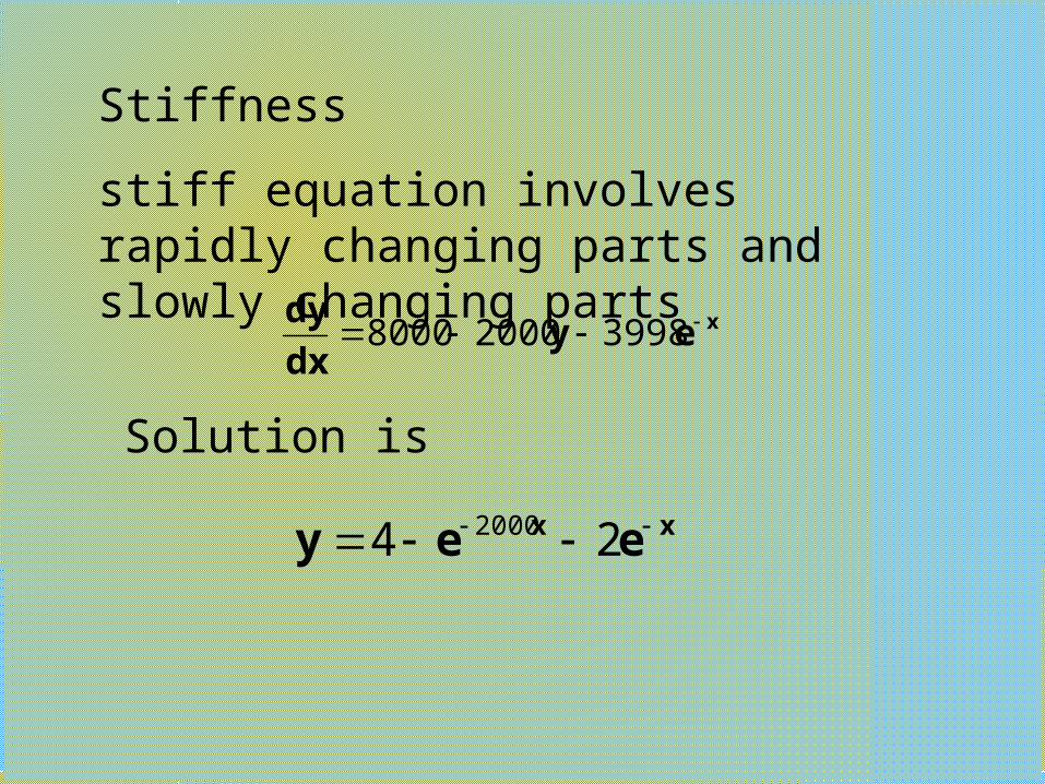
Stiffness
stiff equation involves rapidly changing parts and slowly changing parts
xeydx
dy 399820008000
xx eey 24 2000
Solution is

0
0.5
1
1.5
2
2.5
3
3.5
4
0 0.5 1 1.5 2 2.5
0
0.5
1
1.5
2
2.5
3
-0.001 0.001 0.003 0.005 0.007 0.009 0.011 0.013 0.015

Look at homogeneous part of equation
ydx
dy2000
aydx
dy
In general
Explicit Euler’s method
hayyhdx
dyyy ii
iii 1

ahy
hayyy
i
iii
11
Look at what happens to y over long time - stability
If then y goes to infinity
So for explicit method to work - small h
11 ah
11 ah
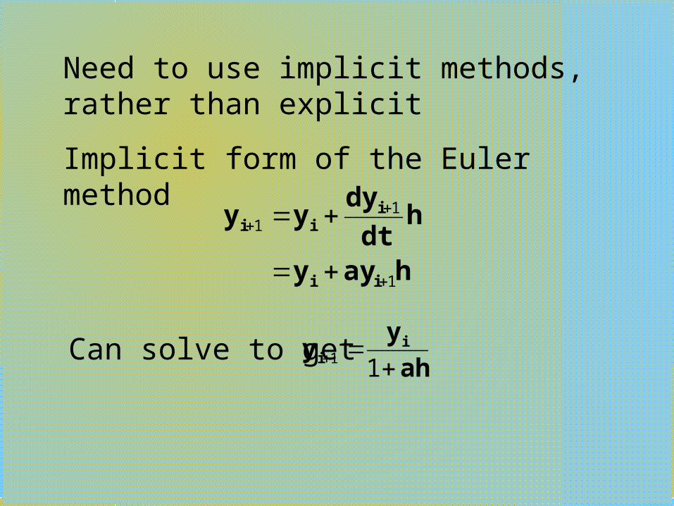
Need to use implicit methods, rather than explicit
Implicit form of the Euler method
hayy
hdt
dyyy
ii
iii
1
11
Can solve to getah
yy ii
11
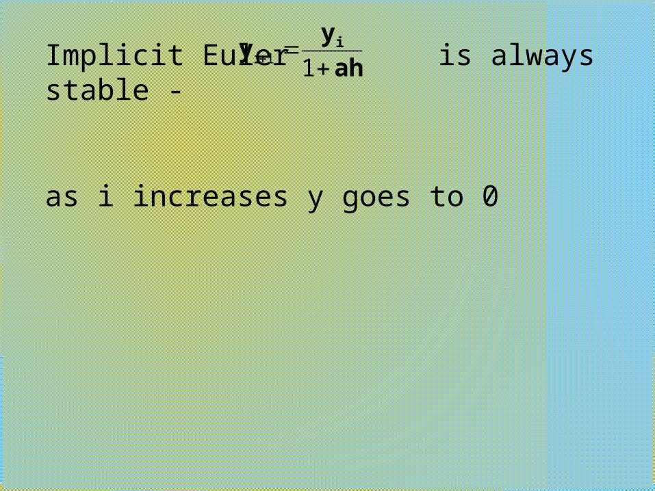
Implicit Euler is always stable -
as i increases y goes to 0
ah
yy ii
11

Example: xeydx
dy 399820008000
Explict solution:
since a is 2000, let h=0.0001
0
0.5
1
1.5
2
2.5
0 0.01 0.02 0.03 0.04 0.05 0.06
y
yExplicit
heyyyhdx
dyyy ix
iiii
ii *39982000800011
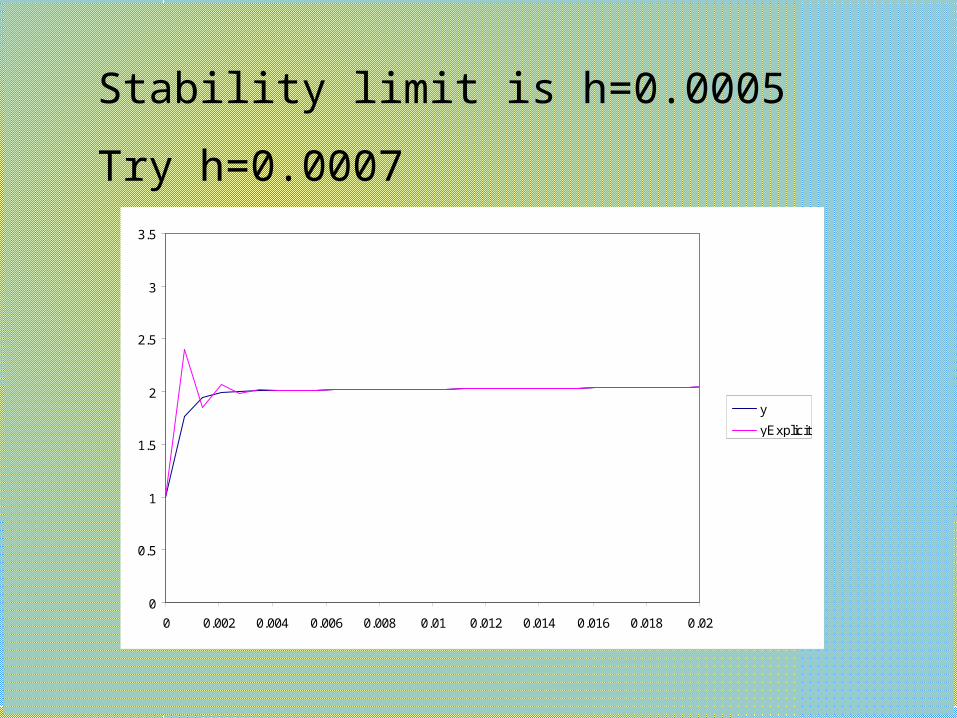
Stability limit is h=0.0005
Try h=0.0007
0
0.5
1
1.5
2
2.5
3
3.5
0 0.002 0.004 0.006 0.008 0.01 0.012 0.014 0.016 0.018 0.02
y
yExplicit
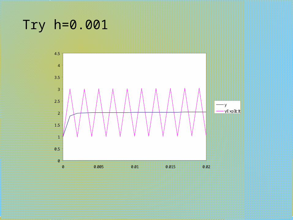
Try h=0.001
0
0.5
1
1.5
2
2.5
3
3.5
4
4.5
0 0.005 0.01 0.015 0.02
y
yExplicit

h=0.002
-15
-10
-5
0
5
10
15
0 0.005 0.01 0.015 0.02 0.025
sig
n o
f y
* ln
ofa
bs(
y v
alu
e)
lny
lnyExplicit

Implicit approach:
h
hehyy
heyy
ydx
dyyy
i
i
xi
i
xii
ii
ii
20001
39988000
*3998200080001
1
1
1
11
1

h=0.002
0
0.5
1
1.5
2
2.5
3
3.5
4
4.5
0 0.005 0.01 0.015 0.02
0
0.5
1
1.5
2
2.5
3
3.5
4
4.5
0 0.5 1 1.5 2 2.5 3
y
yImplicit


