

Advanced Computing for Engineering Applications
© Dan Negrut, 2013UW-Madison
Dan Negrut
Simulation-Based Engineering Lab
Wisconsin Applied Computing Center
Department of Mechanical Engineering
Department of Electrical and Computer Engineering
University of Wisconsin-Madison
Milano
18-23 November
2013

� Old: Power is free, Transistors expensive
� New: Power expensive, Transistors free (Can put more on chip than can afford to turn on)
� Old: Multiplies are slow, Memory access is fast
� New: Memory slow, multiplies fast [“Memory wall”](400-600 cycles for DRAM memory access, 1 clock for FMA)
� Old : Increasing Instruction Level Parallelism via compilers, innovation (Out-of-order, speculation, VLIW, …)
� New: “ILP wall” diminishing returns on more ILP
� New: Power Wall + Memory Wall + ILP Wall = Brick Wall� Old: Uniprocessor performance 2X / 1.5 yrs
� New: Uniprocessor performance only 2X / 5 yrs?
Conventional Wisdomin Computer Architecture
2

Summarizing It All…
� The sequential execution model is losing steam
� The bright spot: number of transistors per unit area going up and up
3

� OK, now what?
4
Moore’s Law
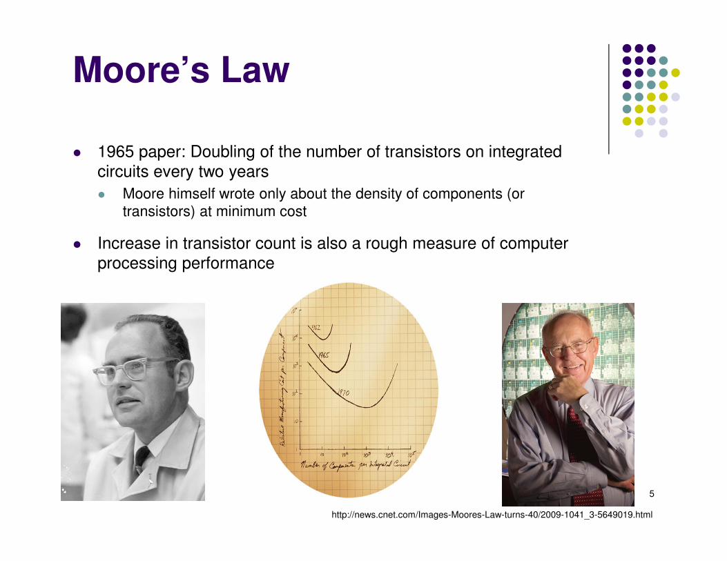
� 1965 paper: Doubling of the number of transistors on integrated circuits every two years
� Moore himself wrote only about the density of components (or transistors) at minimum cost
� Increase in transistor count is also a rough measure of computer processing performance
http://news.cnet.com/Images-Moores-Law-turns-40/2009-1041_3-5649019.html
5

Moore’s Law (1965)
� “The complexity for minimum component costs has increased at arate of roughly a factor of two per year (see graph on next page).Certainly over the short term this rate can be expected to continue, ifnot to increase. Over the longer term, the rate of increase is a bitmore uncertain, although there is no reason to believe it will notremain nearly constant for at least 10 years. That means by 1975,the number of components per integrated circuit for minimum costwill be 65,000. I believe that such a large circuit can be built on asingle wafer.”
“Cramming more components onto integrated circuits” by Gordon E. Moore, Electronics, Volume 38, Number 8, April 19, 1965
6

Intel Roadmap
� 2013 – 22 nm
� 2015 – 14 nm
� 2017 – 10 nm
� 2019 – 7 nm
� 2021 – 5 nm
� 2023 – ??? (your turn, maybe carbon nanotubes)
7

Many-core array
• CMP with 10s-100s low power cores
• Scalar cores
• Capable of TFLOPS+
• Full System-on-Chip
• Servers, workstations, embedded…
Dual core
• Symmetric multithreading
Multi-core array
• CMP with ~10 cores
Large, Scalar cores for high single-thread performance
Scalar plus many core for highly threaded workloads
Intel’s Vision: Evolutionary Configurable Architecture
Micro2015: Evolving Processor Architecture, Intel® Developer Forum, March 2005
CMP = “chip multi-processor”
Presentation Paul Petersen,Sr. Principal Engineer, Intel
8

Parallel Computing: Here to Stay for This Decade
� More transistors = More computational units
� November 2013:
� Intel Xeon w/ 12 cores – 3 billion transistors
� Projecting ahead:
� 2015: 24 cores
� 2017: about 50 cores
� 2019: about 100 cores
� 2021: about 200 cores
11/19/2013

Old School
� Increasing clock frequency is primary method of performance improvement
� Processors parallelism is primary method of performance improvement
� Don’t bother parallelizing an application, just wait and run on much faster sequential computer
� Nobody is building one processor per chip. This marks the end of the La-Z-Boy programming era
� Less than linear scaling for a multiprocessor is failure
� Given the switch to parallel hardware, even sub-linear speedups are beneficial as long as you beat the sequential
New School
Slide Source: Berkeley View of Landscape
10

Moving Into Parallelism…
11

From Simple to Complex: Part 1
� The von Neumann architecture
12

From Simple to Complex:Part 2
� The architecture of the early to mid 1990s
� Pipelining was king
13

From Simple to Complex:Part 3
� The architecture of late 1990s, early 2000s
� ILP galore
14

Two Examples of Parallel HW
� Intel Haswell� Multicore architecture
� NVIDIA Fermi� Large number of scalar processors (“shaders”)
15

Intel Haswell
� June 2013
� 22 nm technology
� 1.4 billion transistors
� 4 cores, hyperthreaded
� Integrated GPU
� System-on-a-chip design
16

The Fermi Architecture
� Late 2009, early 2010
� 40 nm technology
� Three billion transistors
� 512 Scalar Processors (SP, “shaders”)
� L1 cache
� L2 cache
� 6 GB of global memory
� Operates at low clock rate
� High bandwidth (close to 200 GB/s)
17

Fermi: 30,000 Feet Perspective
� Lots of ALU (green), not much of CU
� Explains why GPUs are fast for high arithmetic intensity applications
� Arithmetic intensity: high when many operations performed per word of memory
18

“Big Iron” Parallel Computing
19

Euler: CPU/GPU Heterogeneous Cluster~ Hardware Configuration ~
20

Euler, in reality…
21

Overview of Large Multiprocessor Hardware Configurations (“Big Iron”)
Courtesy of Elsevier, Computer Architecture, Hennessey and Patterson, fourth edition
Euler
22

Some Nomenclature…
� Shared addressed space: when you invoke address “0x0043fc6f” on one machine and then invoke “0x0043fc6f” on a different machine they actually point to the same global memory space� Issues: memory coherence
� Fix: software-based or hardware-based
� Distributed addressed space: the opposite of the above
� Symmetric Multiprocessor (SMP): you have one machine that shares amongst all its processing units a certain amount of memory (same address space)� Mechanisms should be in place to prevent data hazards (RAW, WAR, WAW). Brings back the
issue of memory coherence
� Distributed shared memory (DSM): � Also referred to as distributed global address space (DGAS)
� Although physically memory is distributed, it shows as one uniform memory
� Memory latency is highly unpredictable
23

Example
� Distributed-memory multiprocessor architecture (Euler, for instance)
Courtesy of Elsevier, Computer Architecture, Hennessey and Patterson, fourth edition24
Comments, distributed-memory multiprocessor architecture
� Basic architecture consists of nodes containing a processor, some memory, typically some I/O, and an interface to an interconnection network that connects all the nodes
� Individual nodes may contain a small number of processors, which may be interconnected by a small bus or a different interconnection technology, which is less scalable than the global interconnection network
� Popular interconnection network: Mellanox and Qlogic InfiniBand� Bandwidth range: 1 through 50 Gb/sec
� Latency: in the microsecond range (approx. 1E-6 seconds)
� Requires special network cards: HCA – “Host Channel Adaptor”
� InfiniBand offers point-to-point bidirectional serial links intended for the connection of processors with high-speed peripherals such as disks. � Basically, a protocol and implementation for communicating data very fast
� It supports several signaling rates and, as with PCI Express, links can be bonded together for additional throughput
� Similar technologies: Fibre Channel, PCI Express, Serial ATA, etc.
� Euler: uses 4X Infiniband QDR for 40 Gb/sec bandwidth 25

Example, SMP[This is not “Big Iron”, rather a desktop nowadays]
� Shared-Memory Multiprocessor Architecture
Courtesy of Elsevier, Computer Architecture, Hennessey and Patterson, fourth edition
Usually SRAM
Usually DRAM
26

Comments, SMP Architecture
� Multiple processor-cache subsystems share the same physical off-chip memory
� Typically connected to this off-chip memory by one or more buses or a switch
� Key architectural property: uniform memory access (UMA) time to all of memory from all the processors
� This is why it’s called symmetric
27

Examples…
� Shared-Memory � Intel Xeon Phi available as of 2012
� Packs 61 cores, which are on the basic (unsophisticated) side
� AMD Opteron 6200 Series (16 cores: Opteron 6276) – Bulldozer architecture
� Sun Niagara
� Distributed-Memory� IBM BlueGene/L
� Cell (see http://users.ece.utexas.edu/~adnan/vlsi-07/hofstee-cell.ppt)
28

Big Iron: Where Are We Today?[Info lifted from Top500 website: http://www.top500.org/]
29

Big Iron: Where Are We Today?[Cntd.]
� Abbreviations/Nomenclature� MPP – Massively Parallel Processing
� Constellation – subclass of cluster architecture envisioned to capitalize on data locality
� MIPS – “Microprocessor without Interlocked Pipeline Stages”, a chip design of the MIPS Computer Systems of Sunnyvale, California
� SPARC – “Scalable Processor Architecture” is a RISC instruction set architecture developed by Sun Microsystems (now Oracle) and introduced in mid-1987
� Alpha - a 64-bit reduced instruction set computer (RISC) instruction set architecture developed by DEC (Digital Equipment Corporation was sold to Compaq, which was sold to HP) – adopted by Chinese chip manufacturer (see primer)
30

Short Digression [second take]:
What is a MPP?
� A very large-scale comp. system with commodity processing nodes interconnected with a high-speed low-latency interconnect
� Memories are physically distributed� Nodes often run a microkernel� Contains one host monolithic OS� There are overlaps among MPPs, clusters, and SMPs
[Youngdae Kim ]→
31
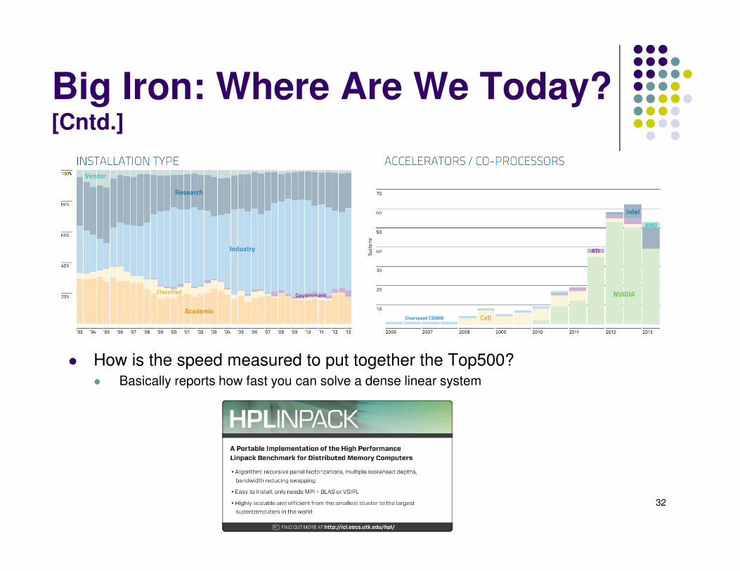
Big Iron: Where Are We Today?[Cntd.]
� How is the speed measured to put together the Top500?� Basically reports how fast you can solve a dense linear system
32

Flynn’s Taxonomy of Architectures
� SISD - Single Instruction/Single Data
� SIMD - Single Instruction/Multiple Data
� MISD - Multiple Instruction/Single Data
� MIMD - Multiple Instruction/Multiple Data
� There are several ways to classify architectures (we just saw on based on how memory is organized/accessed)
� Below, classified based on how instructions are executed in relation to data
33

Single Instruction/Single DataArchitectures
Your desktop, before the spread of dual core CPUs
Slide Source: Wikipedia, Flynn’s Taxonomy
PU – Processing Unit
34

Flavors of SISD
Instructions:
35

Single Instruction/Multiple DataArchitectures
Processors that execute same instruction on multiple pieces of data: NVIDIA GPUs
Slide Source: Wikipedia, Flynn’s Taxonomy
36

Single Instruction/Multiple Data[Cntd.]
� Each core runs the same set of instructions on different data� Examples:
� Graphics Processing Unit (GPU): processes pixels of an image in parallel� CRAY’s vector processor, see image below
Slide Source: Klimovitski & Macri, Intel
37

SISD versus SIMD
Writing a compiler for SIMD architectures is difficult (inter-thread communication complicates the picture…)
Slide Source: ars technica, Peakstream article
38

Multiple Instruction/Single Data
Not useful, not aware of any commercial implementation…
Slide Source: Wikipedia, Flynn’s Taxonomy
39

Multiple Instruction/Multiple Data
As of 2006, all the top 10 and most of the TOP500 supercomputers were based on a MIMD architecture
Slide Source: Wikipedia, Flynn’s Taxonomy
40

Multiple Instruction/Multiple Data
� The sky is the limit: each PU is free to do as it pleases
� Can be of either shared memory or distributed memory categories
Instructions:
41

Amdahl's Law
“A fairly obvious conclusion which can be drawn at this point is that the effort expended on achieving high parallel processing rates is wasted unless it is accompanied by achievements in sequential processing rates of very nearly the same magnitude”
Excerpt from “Validity of the single processor approach to achieving large
scale computing capabilities,” by Gene M. Amdahl, in Proceedings of the
“AFIPS Spring Joint Computer Conference,” pp. 483, 1967
42

Amdahl’s Law[Cntd.]
� Sometimes called the law of diminishing returns
� In the context of parallel computing used to illustrate how going parallel with a part of your code is going to lead to overall speedups
� The art is to find for the same problem an algorithm that has a large rp
� Sometimes requires a completely different angle of approach for a solution
� Nomenclature� Algorithms for which rp=1 are called “embarrassingly parallel”
43

Example: Amdahl's Law
� Suppose that a program spends 60% of its time in I/O operations, pre and post-processing
� The rest of 40% is spent on computation, most of which can be parallelized
� Assume that you buy a multicore chip and can throw 6 parallel threads at this problem. What is the maximum amount of speedup that you can expect given this investment?
� Asymptotically, what is the maximum speedup that you can ever hope for?
44

A Word on “Scaling”[important to understand]
� Algorithmic Scaling of a solution algorithm
� You only have a mathematical solution algorithm at this point
� Refers to how the effort required by the solution algorithm scales with the size of the problem
� Examples:
� Naïve implementation of the N-body problem scales like O(N2), where N is the number of bodies
� Sophisticated algorithms scale like O(N¢logN)
� Gauss elimination scales like the cube of the number of unknowns in your linear system
� Implementation Scaling on a certain architecture
� Intrinsic Scaling: how the wall-clock run time changes with an increase in the size of the problem
� Strong Scaling: how the wall-clock run time changes when you increase the processing resources
� Weak Scaling: how the wall-clock run time changes when you increase the problem size but also the processing resources in a way that basically keeps the ration of problem size/processor constant
� A thing you should worry about: is the Intrinsic Scaling similar to the Algorithmic Scaling?
� If Intrinsic Scaling significantly worse than Algorithmic Scaling:
� You might have an algorithm that thrashes the memory badly, or
� You might have a sloppy implementation of the algorithm 45

End: Intro Part
Beginning: GPU Computing, CUDA Programming Model
46

Layout of Typical Hardware ArchitectureCPU
(the “host”)GPU w/
local DRAM
(the “device”)
47Wikipedia

Parallel Computing on a GPU
� NVIDIA GPU Computing Architecture� Via a separate HW interface
� In laptops, desktops, workstations, servers
� Kepler K20X delivers 1.515 Tflops in double precision
� Multithreaded SIMT model uses application data parallelism and thread parallelism
� Programmable in C with CUDA tools� “Extended C”
Tesla C2050
Kepler K20X
48

Bandwidth in a CPU-GPU System
[Robert Strzodka, Max Plank Institute, Germany]→49
1-8 GB/s
GPUNOTE: The width
of the black lines is
proportional to the
bandwidth.

GPU vs. CPU – Memory Bandwidth[GB/sec]
50
0
20
40
60
80
100
120
140
160
2003 2004 2005 2006 2007 2008 2009 2010
Tesla 8-series
Tesla 10-series
Nehalem 3 GHz
Westmere3 GHz
Tesla 20-series
GB
/Sec
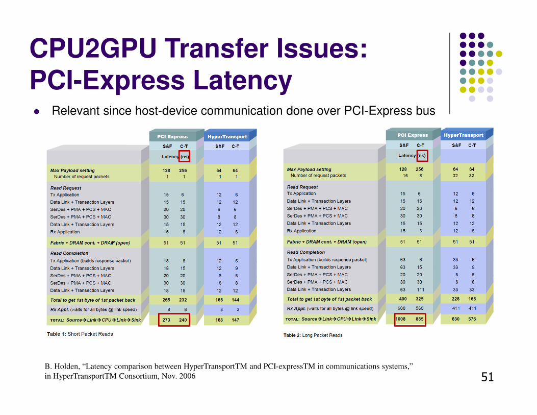
CPU2GPU Transfer Issues:PCI-Express Latency
B. Holden, “Latency comparison between HyperTransportTM and PCI-expressTM in communications systems,”
in HyperTransportTM Consortium, Nov. 2006 51
� Relevant since host-device communication done over PCI-Express bus

Comparison:Latency, DRAM Memory Access
52
Courtesy of Elsevier, Computer Architecture, Hennessey and Patterson, fourth edition

0
200
400
600
800
1000
1200
2003 2004 2005 2006 2007 2008 2009 2010
Tesla 8-series
Tesla 10-series
Nehalem3 GHz
Tesla 20-series
Westmere3 GHz
Tesla 20-series
Tesla 10-series
CPU vs. GPU – Flop Rate(GFlops)
53
Single Precision
Double Precision
GF
lop
/Sec

54
More Up-to-Date, DP Figures…
Source: Revolutionizing High Performance Computing / Nvidia Tesla

What is the GPU so Fast?
� The GPU is specialized for compute-intensive, highly data parallel computation (owing to its graphics rendering origin)
� More transistors can be devoted to data processing rather than data caching and control flow
� Where are GPUs good: high arithmetic intensity (the ratio between arithmetic operations and memory operations)
� The fast-growing video game industry exerts strong economic pressure that forces constant innovation
DRAM
Cache
ALUControl
ALU
ALU
ALU
DRAM
CPU GPU
55

GPU – NVIDIA Tesla C2050
CPU – Intel core I7 975 Extreme
Processing Cores 448 4 (8 threads)
Memory 3 GB - 32 KB L1 cache / core
- 256 KB L2 (I&D)cache / core
- 8 MB L3 (I&D) shared by all cores
Clock speed 1.15 GHz 3.20 GHz
Memory bandwidth 140 GB/s 25.6 GB/s
Floating point operations/s
515 x 109
Double Precision
70 x 109
Double Precision
Key ParametersGPU, CPU
56

When Are GPUs Good?
� Ideally suited for data-parallel computing (SIMD)
� Moreover, you want to have high arithmetic intensity
� Arithmetic intensity: ratio or arithmetic operations to memory operations
� Example: quick back-of-the-envelope computation to illustrate the crunching number power of a modern GPU� Suppose it takes 4 microseconds (4E-6) to launch a kernel (more about this later…)
� Suppose you own a 1 Tflops (1E12) Fermi-type GPU and use to add (in 4 cycles) floats
� Then, you have to carry out about 1 million floating point ops on the GPU to break even with the amount of time it took you to invoke execution on the GPU in the first place
57

When Are GPUs Good?[Cntd.]
� Another quick way to look at it: � Your 1 Tflops GPU needs a lot of data to keep busy and reach that peak rate
� For instance: assume that you want to add different numbers and reach 1 Tflops: 1E12 ops/second…
� You need to feed 2E12 operands per second…
� If each number is stored using 4 bytes (float), then you need to fetch 2E12*4 bytes in a second. This is 8E12 B/s, which is 8 TB/s…
� The memory bandwidth on the GPU is in the neighborhood of 0.15 TB/s, about 50 times less than what you need (and you haven’t taken into account that you probably want to send back the outcome of the operation that you carry out)
� Here’s a set of rules that you need to keep in mind before going further…� GET THE DATEA ON THE GPU AND KEEP IT THERE
� GIVE THE GPU ENOUGH WORK TO DO
� FOCUS ON DATA REUSE WITHIN THE GPU TO AVOID MEMORY BANDWIDTH LIMITATIONS
58
Rules suggested by Rob Farber

GPU Computing – The Basic Idea
� GPU, going beyond graphics:
� The GPU is connected to the CPU by a reasonable fast bus (8 GB/s is typical today)
� The idea is to use the GPU as a co-processor� Farm out big parallel jobs to the GPU� CPU stays busy with the control of the execution and “corner” tasks� You have to copy data down into the GPU, and then fetch results back
� Ok if this data transfer is overshadowed by the number crunching done using that data (remember Amdahl’s law…)
59

CUDA: Making the GPU Tick…
� “Compute Unified Device Architecture” – freely distributed by NVIDIA
� When introduced it eliminated the constraints associated with GPGPU
� It enables a general purpose programming model
� User kicks off batches of threads on the GPU to execute a function (kernel)
� Targeted software stack
� Scientific computing oriented drivers, language, and tools
� Driver for loading computation programs into GPU
� Standalone Driver - Optimized for computation
� Interface designed for compute, graphics free, API
� Explicit GPU memory management60

CUDA Programming Model:GPU as a Highly Multithreaded Coprocessor
� The GPU is viewed as a compute device that:� Is a co-processor to the CPU or host
� Has its own DRAM (device memory, or global memory in CUDA parlance)
� Runs many threads in parallel
� Data-parallel portions of an application run on the device as kernels which are executed in parallel by many threads
� Differences between GPU and CPU threads � GPU threads are extremely lightweight
� Very little creation overhead
� GPU needs 1000s of threads for full efficiency
� Multi-core CPU needs only a few heavy ones
61HK-UIUC

Fermi: Quick Facts
� Lots of ALU (green), not much of CU
� Explains why GPUs are fast for high arithmetic intensity applications
� Arithmetic intensity: high when many operations performed per word of memory
62

The Fermi Architecture
� Late 2009, early 2010
� 40 nm technology
� Three billion transistors
� 512 Scalar Processors (SP, “shaders”)
� 64 KB L1 cache
� 768 KB L2 uniform cache (shared by all SMs)
� Up to 6 GB of global memory
� Operates at several clock rates� Memory
� Scheduler
� Shader (SP)
� High memory bandwidth � Close to 200 GB/s
63

GPU Processor Terminology
� GPU is a SIMD device → it works on “streams” of data� Each “GPU thread” executes one general instruction on the stream of
data that it is assigned to handle� The NVIDIA calls this model SIMT (single instruction multiple thread)
� The number crunching power comes from a vertical hierarchy: � A collection of Streaming Multiprocessors (SMs)� Each SM has a set of 32 Scalar Processors (SPs)
� The quantum of scalability is the SM� The more $ you pay, the more SMs you get inside your GPU� Fermi can have up to 16 SMs on one GPU card
64

Compute Capability [of a Device]vs.
CUDA Version
� “Compute Capability of a Device” refers to hardware� Defined by a major revision number and a minor revision number
� Example: � Tesla C1060 is compute capability 1.3 � Tesla C2050 is compute capability 2.0� Fermi architecture is capability 2 (on Euler now)� Kepler architecture is capability 3 (the highest, on Euler now)� The minor revision number indicates incremental changes within an architecture class
� A higher compute capability indicates an more able piece of hardware
� The “CUDA Version” indicates what version of the software you are using to run on the hardware� Right now, the most recent version of CUDA is 5.5
� In a perfect world � You would run the most recent CUDA (version 5.5) software release� You would use the most recent architecture (compute capability 3.0)
65

Compatibility Issues
� The basic rule: the CUDA Driver API is backward, but not forward compatible� Makes sense, the functionality in later versions increased, was not
there in previous versions
66
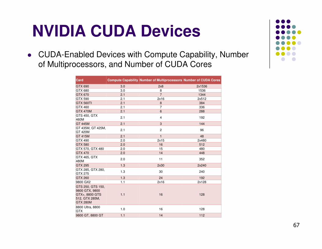
NVIDIA CUDA Devices
� CUDA-Enabled Devices with Compute Capability, Number of Multiprocessors, and Number of CUDA Cores
67
Card Compute Capability Number of Multiprocessors Number of CUDA Cores
GTX 690 3.0 2x8 2x1536
GTX 680 3.0 8 1536
GTX 670 2.1 7 1344
GTX 590 2.1 2x16 2x512
GTX 560TI 2.1 8 384
GTX 460 2.1 7 336
GTX 470M 2.1 6 288
GTS 450, GTX 460M
2.1 4 192
GT 445M 2.1 3 144
GT 435M, GT 425M, GT 420M
2.1 2 96
GT 415M 2.1 1 48
GTX 490 2.0 2x15 2x480
GTX 580 2.0 16 512
GTX 570, GTX 480 2.0 15 480
GTX 470 2.0 14 448
GTX 465, GTX 480M
2.0 11 352
GTX 295 1.3 2x30 2x240
GTX 285, GTX 280, GTX 275
1.3 30 240
GTX 260 1.3 24 192
9800 GX2 1.1 2x16 2x128
GTS 250, GTS 150, 9800 GTX, 9800 GTX+, 8800 GTS 512, GTX 285M, GTX 280M
1.1 16 128
8800 Ultra, 8800 GTX
1.0 16 128
9800 GT, 8800 GT 1.1 14 112

The CUDA Execution Model

GPU Computing – The Basic Idea
� The GPU is linked to the CPU by a reasonably fast connection
� The idea is to use the GPU as a co-processor
� Farm out big parallel tasks to the GPU
� Keep the CPU busy with the control of the execution and “corner” tasks
69

The CUDA Way: Extended C
� Declaration specifications:
� global, device, shared, local, constant
� Keywords
� threadIdx, blockIdx
� Intrinsics
� __syncthreads
� Runtime API
� Functions for memory and execution management
� Kernel launch
70HK-UIUC
__device__ float filter[N];
__global__ void convolve (float *image) {
__shared__ float region[M];
...
region[threadIdx.x] = image[i];
...
__syncthreads()
...
image[j] = result;
}
// Allocate GPU memory
void *myimage = cudaMalloc(bytes)
// 100 blocks, 10 threads per block
convolve<<<100, 10>>> (myimage);

Example: Hello World!
� Standard C that runs on the host
� NVIDIA compiler (nvcc) can be
used to compile programs with no device code
71
int main(void) {
printf("Hello World!\n");
return 0;
}
Output, on Euler:
$ nvcc hello_world.cu
$ a.out
Hello World!
$
Note the “cu” suffix
[NVIDIA]→

Compiling with nvcc for CUDA
� Source files with CUDA language extensions must be compiled with nvcc
� You spot such a file by its .cu or .cuh suffixes
� Example:
>> nvcc -arch=sm_20 foo.cu
� nvcc is actually a compile driver
� Works by invoking all the necessary tools and compilers like g++, cl, ...
� nvcc can output:
� C code� Must then be compiled with the rest of the application using another tool
� ptx code (CUDA’s assembly language, device independent)
� Or directly object code (cubin)
72

� Two new syntactic elements…
73
__global__ void mykernel(void) {
}
int main(void) {
mykernel<<<1,1>>>();
printf("Hello World!\n");
return 0;
}
Hello World! with Device Code
[NVIDIA]→

Hello World! with Device Code
� CUDA C/C++ keyword __global__ indicates a function that:
� Runs on the device
� Is called from host code
� People refer to it as being a “kernel”
� nvcc separates source code into host and device components
� Device functions, e.g. mykernel(), processed by NVIDIA compiler
� Host functions, e.g. main(), processed by standard host compiler� gcc, cl.exe
__global__ void mykernel(void) {
}
[NVIDIA]→

Hello World! with Device Code
� Triple angle brackets mark a call from host code to device code
� Also called a “kernel launch”
� NOTE: we’ll return to the above (1,1) parameters soon
� That’s all that is required to execute a function on the GPU…
mykernel<<<1,1>>>();
[NVIDIA]→

Hello World! with Device Code
� Actually, mykernel() does not do anything yet...
__global__ void mykernel(void) {
}
int main(void) {
mykernel<<<1,1>>>();
printf("Hello World!\n");
return 0;
}
Output, on Euler:
$ nvcc hello.cu
$ a.out
Hello World!
$
[NVIDIA]→

CUDA: This is it…

Compiling CUDA Code[with nvcc driver]
NVCC
C/C++ CUDAApplication
PTX to Target
Compile
K20X … C2050
Target binary code
PTX Code
CPU Code
78

PTX: Parallel Thread eXecution
� PTX: a pseudo-assembly language used in CUDA programming environment.
� nvcc translates code written in
CUDA’s C into PTX
� nvcc subsequently invokes a
compiler which translates the PTX into a binary code which can be run on a certain GPU
79
__global__ void fillKernel(int *a, int n)
{
int tid = blockIdx.x*blockDim.x + threadIdx.x;
if (tid < n) {
a[tid] = tid;
}
}
.entry _Z10fillKernelPii (
.param .u64 __cudaparm__Z10fillKernelPii_a,
.param .s32 __cudaparm__Z10fillKernelPii_n)
{
.reg .u16 %rh<4>;
.reg .u32 %r<6>;
.reg .u64 %rd<6>;
.reg .pred %p<3>;
.loc 14 5 0
$LDWbegin__Z10fillKernelPii:
mov.u16 %rh1, %ctaid.x;
mov.u16 %rh2, %ntid.x;
mul.wide.u16 %r1, %rh1, %rh2;
cvt.u32.u16 %r2, %tid.x;
add.u32 %r3, %r2, %r1;
ld.param.s32 %r4, [__cudaparm__Z10fillKernelPii_n];
setp.le.s32 %p1, %r4, %r3;
@%p1 bra $Lt_0_1026;
.loc 14 9 0
ld.param.u64 %rd1, [__cudaparm__Z10fillKernelPii_a];
cvt.s64.s32 %rd2, %r3;
mul.wide.s32 %rd3, %r3, 4;
add.u64 %rd4, %rd1, %rd3;
st.global.s32 [%rd4+0], %r3;
$Lt_0_1026:
.loc 14 11 0
exit;
$LDWend__Z10fillKernelPii:
}
PTX for fillKernel

The CUDA Execution Model is Asynchronous
80
This is how your
C code looks like
This is how the code gets executed on the hardware in
heterogeneous computing. GPU calls are asynchronous…
Execution of Kernel0
Execution of Kernel1

Languages Supported in CUDA
� Note that everything is done in C
� Yet minor extensions are needed to flag the fact that a function actually represents a kernel, that there are functions that will only run on the device, etc.
� You end up working in “C with extensions”
� FOTRAN is supported, we’ll not cover here though
� There is support for C++ programming (operator overload, new/delete, etc.)
� Not fully supported yet
81

CUDA Function Declarations(the “C with extensions” part)
Executed on the:
Only callable from the:
__device__ float myDeviceFunc() device device
__global__ void myKernelFunc() device host
__host__ float myHostFunc() host host
� __global__ defines a kernel function, launched by host, executed on the device
� Must return void
� For a full list, see CUDA Reference Manual:
http://docs.nvidia.com/cuda/cuda-c-programming-guide/index.html82

__global__ void kernelFoo(...); // declaration
dim3 DimGrid(100, 50); // 5000 thread blocksdim3 DimBlock(4, 8, 8); // 256 threads per block
kernelFoo<<< DimGrid, DimBlock>>>(...your arg list comes here…);
The Concept of Execution Configuration
� A kernel function must be called with an execution configuration:
83
� NOTE: Any call to a kernel function is asynchronous� By default, execution on host doesn’t wait for kernel to finish

Example
� The host call below instructs the GPU to execute the function (kernel) “foo” using 25,600 threads
� Two arguments are passed down to each thread executing the kernel “foo”
� In this execution configuration, the host instructs the device that it is supposed to run 100 blocks each having 256 threads in it
� The concept of block is important since it represents the entity that gets executed by an SM (stream multiprocessor)
84

More on the Execution Model[Some Constraints]
� There is a limitation on the number of blocks in a grid:
� The grid of blocks can be organized as a 3D structure: max of 65535 by 65535 by 65535 grid of blocks (about 280,000 billion blocks)
� Threads in each block:
� The threads can be organized as a 3D structure (x,y,z)
� The total number of threads in each block cannot be larger than 1024
85

Simple Example:Matrix Multiplication
� A straightforward matrix multiplication example that illustrates the basic features of memory and thread management in CUDA programs
� Use only global memory (don’t bring shared memory into picture yet)
� Matrix will be of small dimension, job can be done using one block
� Concentrate on
� Thread ID usage
� Memory data transfer API between host and device
86HK-UIUC

Square Matrix Multiplication Example
� Compute P = M * N � The matrices P, M, N are of size WIDTH x WIDTH
� Assume WIDTH was defined to be 32
� Software Design Decisions:
� One thread handles one element of P
� Each thread will access all the entries in one row of M and one column of N
� 2*WIDTH read accesses to global memory
� One write access to global memory
M
N
P
WID
TH
WID
TH
WIDTH WIDTH
87

Multiply Using One Thread Block
� One Block of threads computes matrix P� Each thread computes one element of P
� Each thread� Loads a row of matrix M
� Loads a column of matrix N
� Perform one multiply and addition for each pair of M and N elements
� Compute to off-chip memory access ratio close to 1:1
� Not that good, acceptable for now…
� Size of matrix limited by the number of threads allowed in a thread block
Grid 1
Block 1
3 2 5 4
2
4
2
6
48
Thread
(2, 2)
width
MP
N
88HK-UIUC
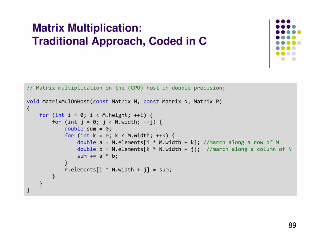
Matrix Multiplication:Traditional Approach, Coded in C
// Matrix multiplication on the (CPU) host in double precision;
void MatrixMulOnHost(const Matrix M, const Matrix N, Matrix P)
{
for (int i = 0; i < M.height; ++i) {
for (int j = 0; j < N.width; ++j) {
double sum = 0;
for (int k = 0; k < M.width; ++k) {
double a = M.elements[i * M.width + k]; //march along a row of M
double b = N.elements[k * N.width + j]; //march along a column of N
sum += a * b;
}
P.elements[i * N.width + j] = sum;
}
}
}
89

Step 1: Matrix Multiplication, Host-side. Main Program Code
int main(void) {
// Allocate and initialize the matrices.
// The last argument in AllocateMatrix: should an initialization with
// random numbers be done? Yes: 1. No: 0 (everything is set to zero)
Matrix M = AllocateMatrix(WIDTH, WIDTH, 1);
Matrix N = AllocateMatrix(WIDTH, WIDTH, 1);
Matrix P = AllocateMatrix(WIDTH, WIDTH, 0);
// M * N on the device
MatrixMulOnDevice(M, N, P);
// Free matrices
FreeMatrix(M);
FreeMatrix(N);
FreeMatrix(P);
return 0;
}
90HK-UIUC

Step 2: Matrix Multiplication [host-side code]
91
void MatrixMulOnDevice(const Matrix M, const Matrix N, Matrix P)
{
// Load M and N to the device
Matrix Md = AllocateDeviceMatrix(M);
CopyToDeviceMatrix(Md, M);
Matrix Nd = AllocateDeviceMatrix(N);
CopyToDeviceMatrix(Nd, N);
// Allocate P on the device
Matrix Pd = AllocateDeviceMatrix(P);
// Setup the execution configuration
dim3 dimGrid(1, 1, 1);
dim3 dimBlock(WIDTH, WIDTH);
// Launch the kernel on the device
MatrixMulKernel<<<dimGrid, dimBlock>>>(Md, Nd, Pd);
// Read P from the device
CopyFromDeviceMatrix(P, Pd);
// Free device matrices
FreeDeviceMatrix(Md);
FreeDeviceMatrix(Nd);
FreeDeviceMatrix(Pd);
}HK-UIUC

// Matrix multiplication kernel – thread specification
__global__ void MatrixMulKernel(Matrix M, Matrix N, Matrix P) {
// 2D Thread Index; computing P[ty][tx]…
int tx = threadIdx.x;
int ty = threadIdx.y;
// Pvalue will end up storing the value of P[ty][tx].
// That is, P.elements[ty * P. width + tx] = Pvalue
float Pvalue = 0;
for (int k = 0; k < M.width; ++k) {
float Melement = M.elements[ty * M.width + k];
float Nelement = N.elements[k * N. width + tx];
Pvalue += Melement * Nelement;
}
// Write matrix to device memory; each thread one element
P.elements[ty * P. width + tx] = Pvalue;
}
Step 4: Matrix Multiplication- Device-side Kernel Function
92
M
N
P
WID
TH
WID
TH
WIDTH WIDTH
tx
ty

// Allocate a device matrix of same size as M.
Matrix AllocateDeviceMatrix(const Matrix M) {
Matrix Mdevice = M;
int size = M.width * M.height * sizeof(float);
cudaMalloc((void**)&Mdevice.elements, size);
return Mdevice;
}
// Copy a host matrix to a device matrix.
void CopyToDeviceMatrix(Matrix Mdevice, const Matrix Mhost) {
int size = Mhost.width * Mhost.height * sizeof(float);
cudaMemcpy(Mdevice.elements, Mhost.elements, size, cudaMemcpyHostToDevice);
}
// Copy a device matrix to a host matrix.
void CopyFromDeviceMatrix(Matrix Mhost, const Matrix Mdevice) {
int size = Mdevice.width * Mdevice.height * sizeof(float);
cudaMemcpy(Mhost.elements, Mdevice.elements, size, cudaMemcpyDeviceToHost);
}
// Free a device matrix.
void FreeDeviceMatrix(Matrix M) {
cudaFree(M.elements);
}
void FreeMatrix(Matrix M) {
free(M.elements);
}
Step 4: Some Loose Ends
93HK-UIUC

Block and Thread Index (Idx)
� Threads and blocks have indices� Used by each thread the decide
what data to work on (more later)
� Block Index: a triplet of uint
� Thread Index: a triplet of uint
� Why this 3D layout?� Simplifies memory
addressing when processingmultidimensional data
� Handling matrices
� Solving PDEs on subdomains
� …
Device
Grid 1
Block(0, 0)
Block(1, 0)
Block(2, 0)
Block(0, 1)
Block(1, 1)
Block(2, 1)
Block (1, 1)
Thread
(0, 1)
Thread
(1, 1)
Thread
(2, 1)
Thread
(3, 1)
Thread
(4, 1)
Thread
(0, 2)
Thread
(1, 2)
Thread
(2, 2)
Thread
(3, 2)
Thread
(4, 2)
Thread
(0, 0)
Thread
(1, 0)
Thread
(2, 0)
Thread
(3, 0)
Thread
(4, 0)
Courtesy: NVIDIA 94

A Couple of Built-In Variables[Critical in supporting the SIMD parallel computing paradigm]
� It’s essential for each thread to be able to find out the grid and block dimensions and its block index and thread index
� Each thread when executing a kernel has access to the following read-only built-in variables
� threadIdx (uint3) – contains the thread index within a block
� blockDim (dim3) – contains the dimension of the block
� blockIdx (uint3) – contains the block index within the grid
� gridDim (dim3) – contains the dimension of the grid
� [ warpSize (uint) – provides warp size, we’ll talk about this later… ]
95

Thread Index vs. Thread ID[critical in (i) understanding how SIMD is supported in CUDA,
and (ii) understanding the concept of “warp”]
96
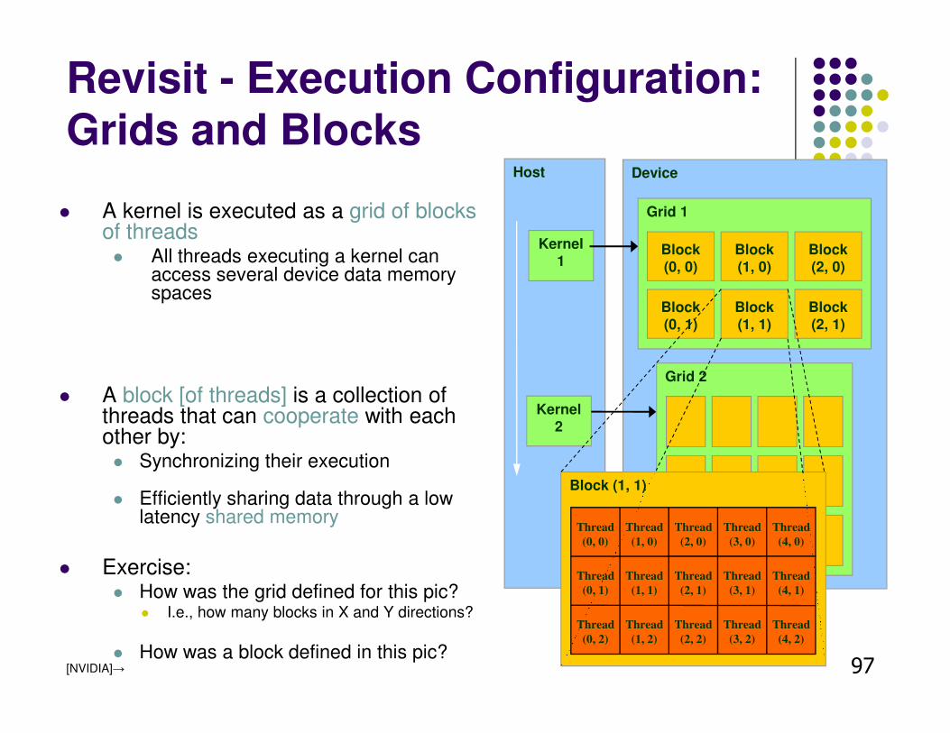
Revisit - Execution Configuration: Grids and Blocks
� A kernel is executed as a grid of blocks of threads� All threads executing a kernel can
access several device data memory spaces
� A block [of threads] is a collection of threads that can cooperate with each other by:� Synchronizing their execution
� Efficiently sharing data through a low latency shared memory
� Exercise:� How was the grid defined for this pic?
� I.e., how many blocks in X and Y directions?
� How was a block defined in this pic?
Host
Kernel 1
Kernel 2
Device
Grid 1
Block(0, 0)
Block(1, 0)
Block(2, 0)
Block(0, 1)
Block(1, 1)
Block(2, 1)
Grid 2
Block (1, 1)
Thread
(0, 1)
Thread
(1, 1)
Thread
(2, 1)
Thread
(3, 1)
Thread
(4, 1)
Thread
(0, 2)
Thread
(1, 2)
Thread
(2, 2)
Thread
(3, 2)
Thread
(4, 2)
Thread
(0, 0)
Thread
(1, 0)
Thread
(2, 0)
Thread
(3, 0)
Thread
(4, 0)
97[NVIDIA]→

� Purpose of Example: see a scenario of how multiple blocks are used to index entries in an array
� First, recall this: there is a limit on the number of threads you can squeeze in a block (up to 1024 of them)
� Note: In the vast majority of applications you need to use many blocks (each of which contains the same number N of threads) to get a job done. This example puts things in perspective
Example: Array Indexing

� With M threads per block a unique index for each thread is given by:
int index = threadIdx.x + blockIdx.x * M;
00 11 7722 33 44 55 66 77 00 11 22 33 44 55 66 77 00 11 22 33 44 55 66 77 00 11 22 33 44 55 66
threadIdx.x threadIdx.x threadIdx.x threadIdx.x
blockIdx.x = 0 blockIdx.x = 1 blockIdx.x = 2 blockIdx.x = 3
� No longer as simple as using only threadIdx.x
� Consider indexing into an array, one thread accessing one element
� Assume you have M=8 threads per block and the array is 32 entries long
[NVIDIA]→
Example: Array Indexing[Important to grasp: shows thread to task mapping]

Example: Array Indexing
� What will be the array entry that thread of index 5 in block of index 2 will work on?
int index = threadIdx.x + blockIdx.x * M;
= 5 + 2 * 8;
= 21;
00 11 7722 33 44 55 66 77 00 11 22 33 44 55 66 77 00 11 22 33 44 5 66 77 00 11 22 33 44 55 66
threadIdx.x = 5
blockIdx.x = 2
M = 8
00 113131
22 33 44 55 66 77 88 99 1010 1111 1212 1313 1414 1515 1616 1717 1818 1919 2020 2121 2222 2323 2424 2525 2626 2727 2828 2929 3030
00 113131
22 33 44 55 66 77 88 99 1010 1111 1212 1313 1414 1515 1616 1717 1818 1919 2020 21 2222 2323 2424 2525 2626 2727 2828 2929 3030
[NVIDIA]→

A Recurring Theme in CUDA Programming[and in SIMD in general]
� Imagine you are one of many threads, and you have your thread index and block index
� You need to figure out what the work you need to do is� Just like we did on previous slide, where thread 5 in block 2 mapped into 21
� You have to make sure you actually need to do that work� In many cases there are threads, typically of large id, that need to do no work
� Example: you launch two blocks with 512 threads but your array is only 1000 elements long. Then 24 threads at the end do nothing
101

Before Moving On…[Some Words of Wisdom]
� In GPU computing you launch as many threads as data items (tasks, jobs) you have to perform� This replaces the purpose in life of the “for” loop
� Number of threads & blocks is established at run-time
� Number of threads = Number of data items (tasks)� It means that you’ll have to come up with a rule to match a thread
to a data item (task) that this thread needs to process
� Solid source of errors and frustration in GPU computing
� It never fails to deliver (frustration)
:-(102

[Sidebar]
Timing Your Application
� Timing support – part of the CUDA API
� You pick it up as soon as you include <cuda.h>
� Why it is good to use
� Provides cross-platform compatibility
� Deals with the asynchronous nature of the device calls by relying on events and forced synchronization
� Reports time in miliseconds, accurate within 0.5 microseconds
� From NVIDIA CUDA Library Documentation:
� Computes the elapsed time between two events (in milliseconds with a resolution of around 0.5 microseconds). If either event has not been recorded yet, this function returns cudaErrorInvalidValue. If either event has been recorded with a non-zero stream, the result is undefined. 103

Timing Example~ Timing a query of device 0 properties ~
104
#include<iostream>
#include<cuda.h>
int main() {
cudaEvent_t startEvent, stopEvent;
cudaEventCreate(&startEvent);
cudaEventCreate(&stopEvent);
cudaEventRecord(startEvent, 0);
cudaDeviceProp deviceProp;
const int currentDevice = 0;
if (cudaGetDeviceProperties(&deviceProp, currentDevice) == cudaSuccess)
printf("Device %d: %s\n", currentDevice, deviceProp.name);
cudaEventRecord(stopEvent, 0);
cudaEventSynchronize(stopEvent);
float elapsedTime;
cudaEventElapsedTime(&elapsedTime, startEvent, stopEvent);
std::cout << "Time to get device properties: " << elapsedTime << " ms\n";
cudaEventDestroy(startEvent);
cudaEventDestroy(stopEvent);
return 0;
}


