
ICCAD 2006 Routing Tutorial
1
Advanced Routing Techniques for Advanced Routing Techniques for Nanometer IC DesignsNanometer IC Designs
Organizer: Organizer: Jason Cong Jason Cong -- Univ. of California, Los Angeles, CAUniv. of California, Los Angeles, CA
Speakers: Speakers: Jason Cong Jason Cong -- Univ. of California, Los Angeles, CAUniv. of California, Los Angeles, CA
Tong Gao Tong Gao -- Synopsys, Inc., Mountain View, CASynopsys, Inc., Mountain View, CARob A. Rob A. RutenbarRutenbar -- Carnegie Mellon Univ., Pittsburgh, PACarnegie Mellon Univ., Pittsburgh, PA
2
Outline
• Introduction• Basic routing algorithms and scalable routing
paradigms (Jason Cong)• Challenges and solutions to large-scale IC
routing in nanometer designs (Tong Gao)• Challenges and solutions to analog and mixed
signal routing (Rob Rutenbar)
ICCAD 2006 Routing Tutorial
2
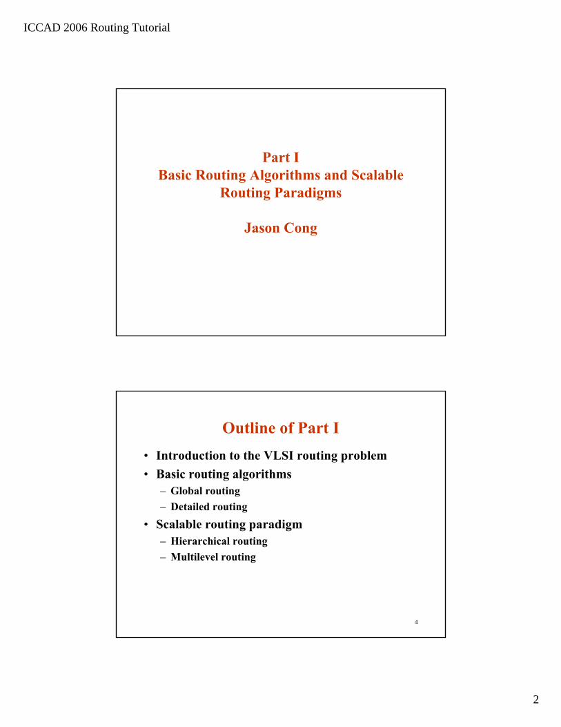
Part I Basic Routing Algorithms and Scalable
Routing Paradigms
Jason Cong
4
Outline of Part I• Introduction to the VLSI routing problem• Basic routing algorithms
– Global routing– Detailed routing
• Scalable routing paradigm– Hierarchical routing– Multilevel routing
ICCAD 2006 Routing Tutorial
3
5
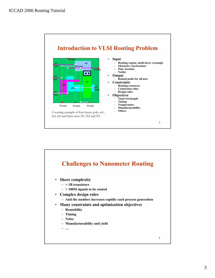
Introduction to VLSI Routing Problem
• Input– Routing region: multi-layer rectangle– Obstacles: size/location– Pins: location– Netlist
• Output– Routed paths for all nets
• Constraints– Routing resources– Connection rules– Design rules
• Objectives– Total wirelength– Timing– Temperature– Manufacturability– Others
poly
m1N1(m1)
N3(m3)
N2(m2)
N3 (m1) N1 m(3) N2 (m2)
N1(poly)
N2(m3)
A routing example of four layers: poly, m1, m2, m3 and three nets: N1, N2 and N3
N2(m2)
m3
N3(m1)
m2
6
Challenges to Nanometer Routing
• Sheer complexity– > 1B transistors– > 100M signals to be routed
• Complex design rules– And the number increases rapidly each process generation
• Many constraints and optimization objectives– Routability– Timing– Noise– Manufacturability and yield– …

ICCAD 2006 Routing Tutorial
4
7
Traditional Two Level Routing FlowFloorplan/Placement Result
Final Layout
…
• Sequential routing• Negotiation-based routing • Iterative deletion• Multicommodity flow-basedGR
DR• Grid-based• Gridless
• shape based• tile based• non-uniform grid graph
8
Global Routing
• Global Routing Problem Formulation• Single Net Routing
– Spanning Tree– Steiner Tree– Rectilinear Steiner Tree
• Routing All Nets– Iterative Improvement– Negotiation Based Routing– Iterative Deletion– Multi-commodity Flow Based Routing
ICCAD 2006 Routing Tutorial
5
9
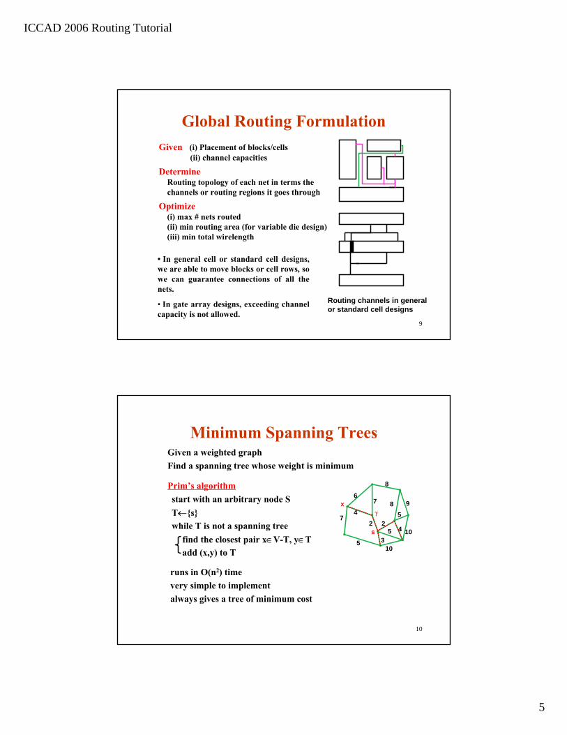
Global Routing FormulationGiven (i) Placement of blocks/cells
(ii) channel capacities
DetermineRouting topology of each net in terms the channels or routing regions it goes through
Optimize(i) max # nets routed(ii) min routing area (for variable die design)(iii) min total wirelength
• In general cell or standard cell designs, we are able to move blocks or cell rows, so we can guarantee connections of all the nets.
• In gate array designs, exceeding channel capacity is not allowed.
Routing channels in general or standard cell designs
10
Minimum Spanning TreesGiven a weighted graphFind a spanning tree whose weight is minimum
Prim’s algorithmstart with an arbitrary node ST←{s}while T is not a spanning tree
find the closest pair x∈V-T, y∈Tadd (x,y) to T
runs in O(n2) time very simple to implementalways gives a tree of minimum cost
8
67
24
7
510
1053
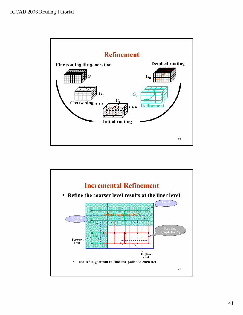
s 4
52
8 9γ
x
ICCAD 2006 Routing Tutorial
6
11
The Graph Minimal Steiner Tree Problem • Input:
– Undirected Graph G=(V,E)– A set of vertices N which is a subset of V– A function cost(e)>0 defined on the edges
• Output:– A tree T(V’,E’) in G, such that
• N is a subset of V’, V’ is a subset of V• E’ is a subset of E
• Objective:– Minimize the sum of cost(e) for each e∈E’
• NP Complete– 1972 , R. Karp formulated a reduction from Exact Cover.– 1979 , S. Even formulated a reduction from Exact Cover by 3-sets
(X3C).
xv∈N
Steiner node/point
w
x
u
12
Graph Steiner Tree Approximate Algorithms
• History– From 1980 to now– Approximate Ratio from 2 to 1.55
• Typical flow – Construct distance graph G’ (N, N×N),
• cost(eij) = cost of shortest path between ni and nj
– Construct Minimum Spanning Tree on G’, MST(G’)– Improve MST(G’)
ICCAD 2006 Routing Tutorial
7
13
KMB Heuristic• [Kou, Markowsky and Berman, Acta Informatica 1981]• Approach
– Construct distance graph G’– Compute MST(G’), expand each edge to the corresponding shortest
path, yielding G’’– Compute MST(G’’) and delete pendant edges from MST(G’’) until
all leaf nodes are in N• Approximate ratio
– 2(1-1/L), where L is the maximum number of leaves in any optimal solution
• Complexity: O(|E|+Vlog|V|)
xv∈N
Steiner node/point
w
x
uv
w
x
u
w(u,v)=d(u,v) G’
τ’
14
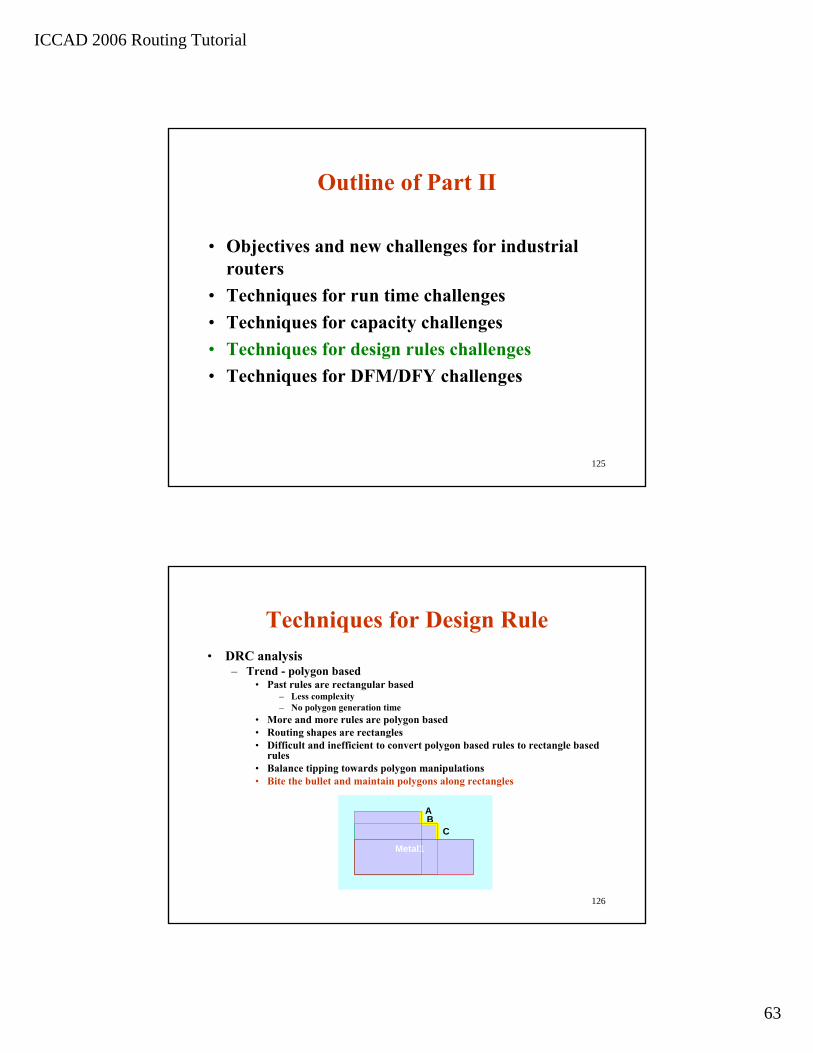
Iterative Improvement
• Alexander and Robins [TCAD96]• Take any Graph Steiner Tree and improve• Definition
– Given a set of Steiner candidate node S ⊆ V-N, define the cost savings of with respect to H
• ∆H(G,N,S)=cost(H(G,N))-cost(H(G,NUS))

ICCAD 2006 Routing Tutorial
8
15
Rectilinear Steiner TreesGiven a set of points on the plane
Determine a Steiner tree using only horizontal and vertical wires( lines)
Manhattan distance:cost(v1,v2) =|x1-x2|+|y1-y2|v1=(x1,y1), v2=(x2,y2)
Steiner points (Hanan grid)Draw a horizontal and a vertical line through each point.Need to consider only grid points as Steiner points
Prim-based algorithm:
Grow a connected subtree by iteratively adding the closest points
It gives 3/2-approximation, i.e. cost(T)≤3/2cost(Topt)
v1=(x1,y1)
v2=(x2,y2)
16
Steiner Tree HeuristicsObservation: MST approximation can be easily improved
Difficulty: where to add Steiner points to maximize sharing??
cost(T)=6 cost(T)=4

ICCAD 2006 Routing Tutorial
9
17
L-Shaped MST ApproachHo, Vijayan and Wong, “ A new approach to the rectilinear steiner tree problem”, DAC’89, pp. 161-166Basic Idea: Each non-degenerated edge in MST has two possible L-shaped layouts. Choose one for each edge in MST to maximize overlap.
degenerated edges non-degenerated edge two L-shaped layouts
MST one L-shaped mapping another L-shaped mapping
Problem: Compute the best L-shaped mapping
18
Key Ideas in L-RST ApproachSeparable MST: bounding boxes of every two non-adjacent edges don’t intersect or overlap
Theorem: Every point set has a separable MSTTheorem: Each node is adjacent to at most 8 edges
(6 non-degenerate edges) in a rectilinear MSTTheorem: We can compute an optimal L-shaped implementation of an MST in O(2d•n) time.
( Dynamic Programming Approach).
Note that d≤8
non-separable MST separable MST
ICCAD 2006 Routing Tutorial
10
19
FLUTE (1)• First proposed for wirelength estimation [Chu, ICCAD04]• Then also used for rectilinear Steiner minimal tree
generation [Chu and Wong, ISPD 2005]• Accurate and fast tree generation for low degree nets • Optimal for nets up to degree 9• Lookup table for low degree nets only, and partition high
degree nets to low degree nets.
20
FLUTE (2)• Lookup Table based Steiner Tree Generation
– with techniques to reduce table size• Net Representation by Vertical Sequence
– index from sorted x position– sequence from sorted y location– Nets with the same vertical sequence share the
same optimal tree solutionVertical sequence = 3142
• Wirelength Representation– linear combination of Hanan grid length– Wirelength vector: vector of the coefficients– Potentially optimal wirelength vector
(POWV): a vector that can potentially produce the optimal wirelength
– Different nets can be represented by the same wirelength vector
Wirelength vector = (1,2,1,1,1,2)
ICCAD 2006 Routing Tutorial
11
21
Global Routing
• Global Routing Problem Formulation• Single Net Routing
– Spanning Tree– Steiner Tree– Rectilinear Steiner Tree
• Routing All Nets– Iterative Improvement– Negotiation Based Routing– Iterative Deletion– Multi-commodity Flow Based Routing
22
Iterative Improvement
• R. Linsker, “An Iterative-Improvement Penalty-Function-Driven Wire Routing System”, p.613-624, IBM Journal of Research and Development Volume 28, Issue 5 (September 1984) Pages: 613 - 624
• Route all nets independently, allowing possible design rule violation
• Iterative ripup and reroute for some or all nets– For both global routing and detailed routing
• Penalty function adjustment before each iteration
ICCAD 2006 Routing Tutorial
12
23
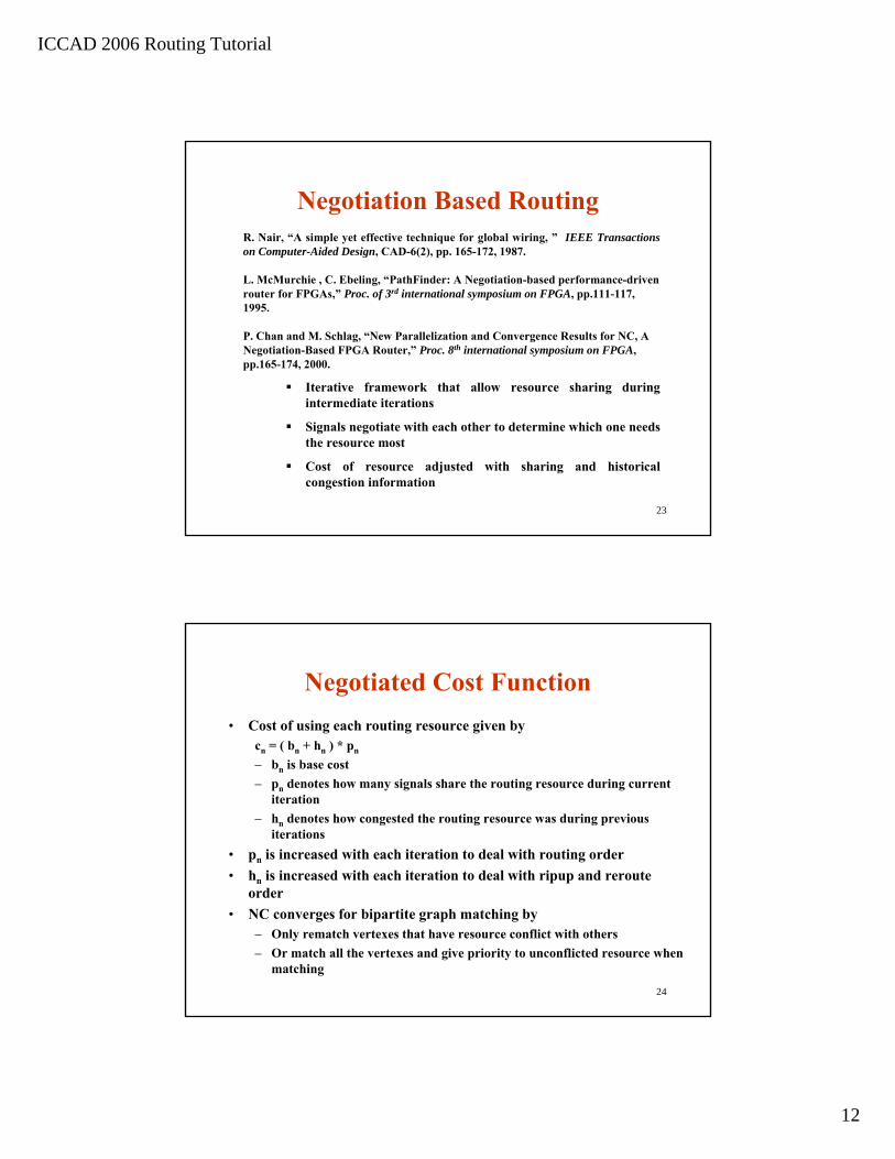
Negotiation Based RoutingR. Nair, “A simple yet effective technique for global wiring, ” IEEE Transactions on Computer-Aided Design, CAD-6(2), pp. 165-172, 1987.
L. McMurchie , C. Ebeling, “PathFinder: A Negotiation-based performance-driven router for FPGAs,” Proc. of 3rd international symposium on FPGA, pp.111-117, 1995.
P. Chan and M. Schlag, “New Parallelization and Convergence Results for NC, A Negotiation-Based FPGA Router,” Proc. 8th international symposium on FPGA, pp.165-174, 2000.
Iterative framework that allow resource sharing during intermediate iterations
Signals negotiate with each other to determine which one needs the resource most
Cost of resource adjusted with sharing and historical congestion information
24
Negotiated Cost Function• Cost of using each routing resource given by
cn = ( bn + hn ) * pn
– bn is base cost– pn denotes how many signals share the routing resource during current
iteration– hn denotes how congested the routing resource was during previous
iterations• pn is increased with each iteration to deal with routing order • hn is increased with each iteration to deal with ripup and reroute
order • NC converges for bipartite graph matching by
– Only rematch vertexes that have resource conflict with others– Or match all the vertexes and give priority to unconflicted resource when
matching
ICCAD 2006 Routing Tutorial
13
25
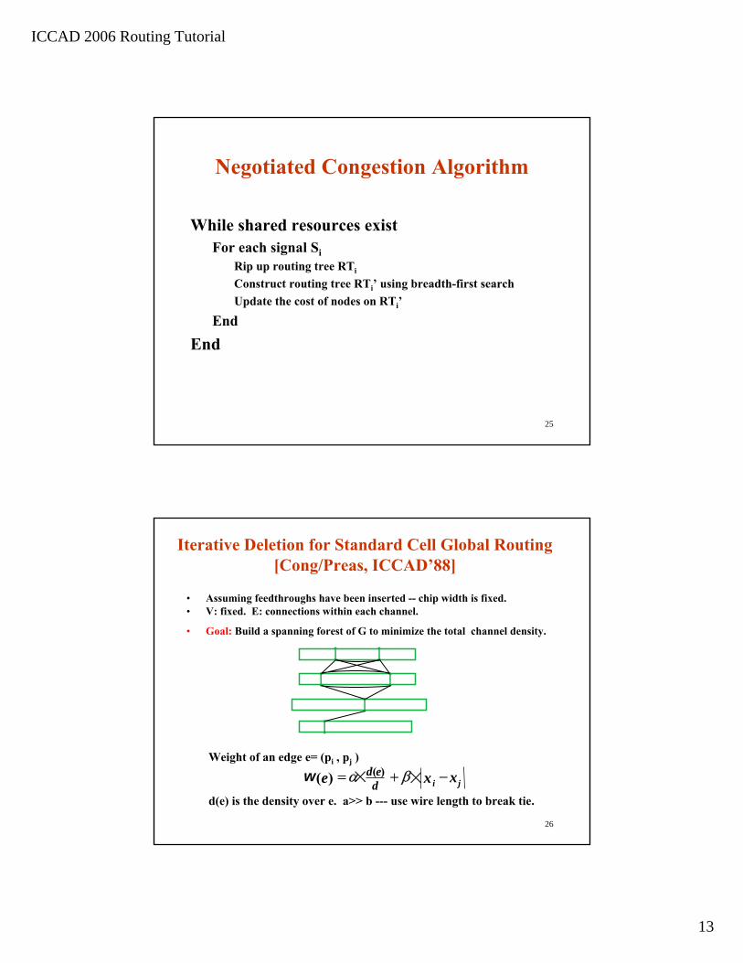
Negotiated Congestion Algorithm
While shared resources existFor each signal Si
Rip up routing tree RTi
Construct routing tree RTi’ using breadth-first searchUpdate the cost of nodes on RTi’
End
End
26
Iterative Deletion for Standard Cell Global Routing[Cong/Preas, ICCAD’88]
• Assuming feedthroughs have been inserted -- chip width is fixed.• V: fixed. E: connections within each channel.
• Goal: Build a spanning forest of G to minimize the total channel density.
Weight of an edge e= (pi , pj )
d(e) is the density over e. a>> b --- use wire length to break tie.
x jided xe −×+×= βαw )()(

ICCAD 2006 Routing Tutorial
14
27
Basic Idea of Iterative DeletionStart with all possible connections. Repeatedly delete the edges
from G until we obtain a spanning forest.
S:= E;repeat
Remove the max weighted edge in S on a cycle;Update edge weights for the affected edges;
until S is a spanning forest;
Advantages Knows the congested area, since we start with all the possible edges (superior to iterative addition).Considers all the edges in every net, each net 'shrinks' to a spanning tree in parallel.There exists a deletion sequence which leads to the optimal spanning forest.
28
Simplified Net Connection Graph
SG=(V’, E’) is a subgraph of G.V’ =V.E’ : connections of adjacent pins of the same net in the same channel.
ICCAD 2006 Routing Tutorial
15
29
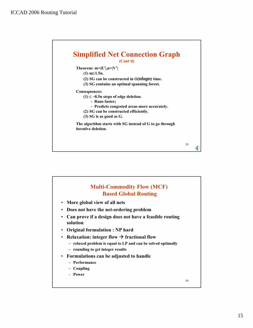
Simplified Net Connection Graph(Cont’d)
Theorem: m=|E’|,n=|V’|(1) m≤1.5n.(2) SG can be constructed in O(nlogn) time.(3) SG contains an optimal spanning forest.
Consequences:(1) ≤ ~0.5n steps of edge deletion.
- Runs faster;- Predicts congested areas more accurately.
(2) SG can be constructed efficiently.(3) SG is as good as G.
The algorithm starts with SG instead of G to go throughiterative deletion.
30
Multi-Commodity Flow (MCF)Based Global Routing
• More global view of all nets• Does not have the net-ordering problem• Can prove if a design does not have a feasible routing
solution• Original formulation : NP hard• Relaxation: integer flow fractional flow
– relaxed problem is equal to LP and can be solved optimally– rounding to get integer results
• Formulations can be adjusted to handle– Performance– Coupling– Power
ICCAD 2006 Routing Tutorial
16
31
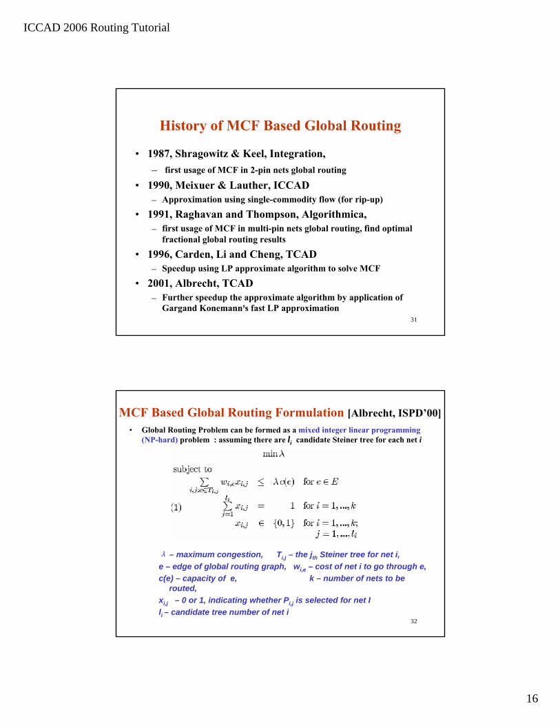
History of MCF Based Global Routing
• 1987, Shragowitz & Keel, Integration,– first usage of MCF in 2-pin nets global routing
• 1990, Meixuer & Lauther, ICCAD– Approximation using single-commodity flow (for rip-up)
• 1991, Raghavan and Thompson, Algorithmica, – first usage of MCF in multi-pin nets global routing, find optimal
fractional global routing results
• 1996, Carden, Li and Cheng, TCAD– Speedup using LP approximate algorithm to solve MCF
• 2001, Albrecht, TCAD– Further speedup the approximate algorithm by application of
Gargand Konemann’s fast LP approximation
32
MCF Based Global Routing Formulation [Albrecht, ISPD’00]• Global Routing Problem can be formed as a mixed integer linear programming
(NP-hard) problem : assuming there are li candidate Steiner tree for each net i
λ – maximum congestion, Ti,j – the jth Steiner tree for net i,e – edge of global routing graph, wi,e – cost of net i to go through e, c(e) – capacity of e, k – number of nets to be
routed,xi,j – 0 or 1, indicating whether Pi,j is selected for net Ili – candidate tree number of net i
ICCAD 2006 Routing Tutorial
17
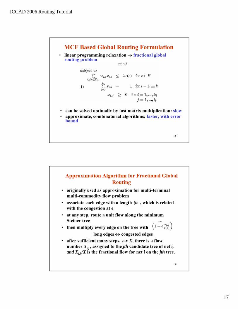
33
MCF Based Global Routing Formulation• linear programming relaxation → fractional global
routing problem
• can be solved optimally by fast matrix multiplication: slow• approximate, combinatorial algorithms: faster, with error
bound
34
Approximation Algorithm for Fractional Global Routing
• originally used as approximation for multi-terminal multi-commodity flow problem
• associate each edge with a length , which is related with the congestion at e
• at any step, route a unit flow along the minimum Steiner tree
• then multiply every edge on the tree with long edges ↔ congested edges
• after sufficient many steps, say X, there is a flow number Xi,j , assigned to the jth candidate tree of net i, and Xi,j /X is the fractional flow for net i on the jth tree.
ICCAD 2006 Routing Tutorial
18
35
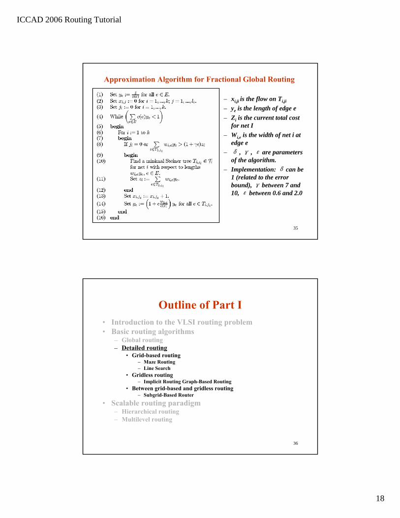
Approximation Algorithm for Fractional Global Routing
– xi,ji is the flow on Ti,ji
– ye is the length of edge e– Zi is the current total cost
for net I– Wi,e is the width of net i at
edge e– δ , γ , ε are parameters
of the algorithm.– Implementation: δ can be
1 (related to the error bound), γ between 7 and 10, ε between 0.6 and 2.0
36
Outline of Part I• Introduction to the VLSI routing problem• Basic routing algorithms
– Global routing– Detailed routing
• Grid-based routing– Maze Routing– Line Search
• Gridless routing– Implicit Routing Graph-Based Routing
• Between grid-based and gridless routing– Subgrid-Based Router
• Scalable routing paradigm– Hierarchical routing– Multilevel routing
ICCAD 2006 Routing Tutorial
19
37
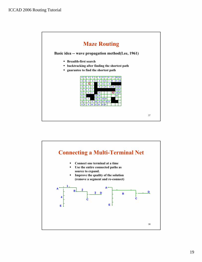
Maze RoutingBasic idea -- wave propagation method(Lee, 1961)
Breadth-first searchbacktracking after finding the shortest pathguarantee to find the shortest path
4 3 2 3 4 5 6 7 8 9 10 11
3 2 1 2 3 4 5 6 7 8 9 10
2 1 A 1 5 6 7 8
3 2 1 2 6 7 8 9 10 11 12
4 3 2 3 12 13
5 4 3 2 14 B 13 14
6 5 13 14 14
7 6 7 11 12 13 14
8 7 8 9 10 11 12 13 14
9 8 9 10 11 12 13 14
38
Connect one terminal at a timeUse the entire connected paths as source to expand.Improve the quality of the solution (remove a segment and re-connect)
4
AD
C
B
E
AD
C
B
E
12
3
Connecting a Multi-Terminal Net
ICCAD 2006 Routing Tutorial
20
39
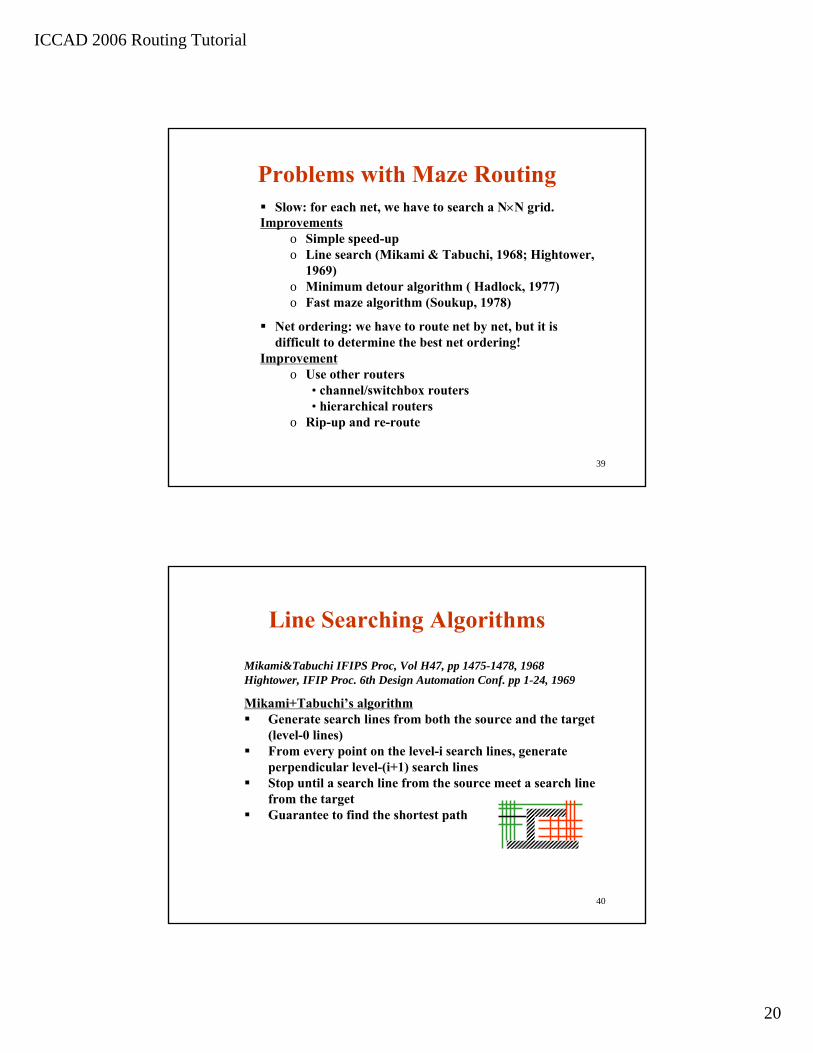
Problems with Maze RoutingSlow: for each net, we have to search a N×N grid.
Improvementso Simple speed-upo Line search (Mikami & Tabuchi, 1968; Hightower,
1969)o Minimum detour algorithm ( Hadlock, 1977)o Fast maze algorithm (Soukup, 1978)
Net ordering: we have to route net by net, but it is difficult to determine the best net ordering!
Improvement o Use other routers
• channel/switchbox routers• hierarchical routers
o Rip-up and re-route
40
Line Searching Algorithms
Mikami&Tabuchi IFIPS Proc, Vol H47, pp 1475-1478, 1968Hightower, IFIP Proc. 6th Design Automation Conf. pp 1-24, 1969
Mikami+Tabuchi’s algorithmGenerate search lines from both the source and the target (level-0 lines)From every point on the level-i search lines, generate perpendicular level-(i+1) search linesStop until a search line from the source meet a search line from the targetGuarantee to find the shortest path
ICCAD 2006 Routing Tutorial
21
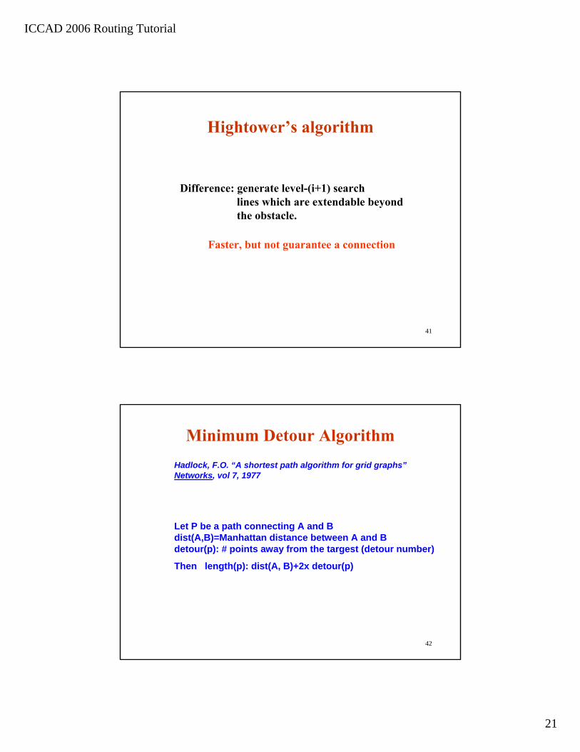
41
Difference: generate level-(i+1) searchlines which are extendable beyondthe obstacle.
Faster, but not guarantee a connection
Hightower’s algorithm
42
Minimum Detour AlgorithmHadlock, F.O. “A shortest path algorithm for grid graphs”Networks, vol 7, 1977
Let P be a path connecting A and Bdist(A,B)=Manhattan distance between A and Bdetour(p): # points away from the targest (detour number)
Then length(p): dist(A, B)+2x detour(p)

ICCAD 2006 Routing Tutorial
22
43
x x xooA
B
obstacle
Detour point
Minimum Detour Algorithm(cont’d)
Algorithmeach cell stores the detour number so far from the source expand the cell with the least detour number
Resultguarantee to find a shortest pathexpand fewer points in general
(similar to the A* search algorithm)
44
Cells Searched Before Target is Reached
(a) original Lee algorithm
(b) minimum detour algorithm
(c) fast maze algorithm
ICCAD 2006 Routing Tutorial
23
45
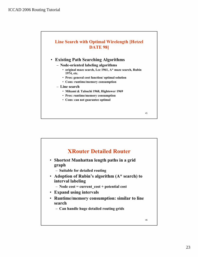
Line Search with Optimal Wirelength [HetzelDATE 98]
• Existing Path Searching Algorithms – Node-oriented labeling algorithms
• original maze search, Lee 1961, A* maze search, Rubin 1974, etc.
• Pros: general cost function/ optimal solution• Cons: runtime/memory consumption
– Line search• Mikami & Tabuchi 1968, Hightower 1969• Pros: runtime/memory consumption• Cons: can not guarantee optimal
46
XRouter Detailed Router• Shortest Manhattan length paths in a grid
graph– Suitable for detailed routing
• Adoption of Rubin’s algorithm (A* search) to interval labeling– Node cost = current_cost + potential cost
• Expand using intervals• Runtime/memory consumption: similar to line
search– Can handle huge detailed routing grids
ICCAD 2006 Routing Tutorial
24
47
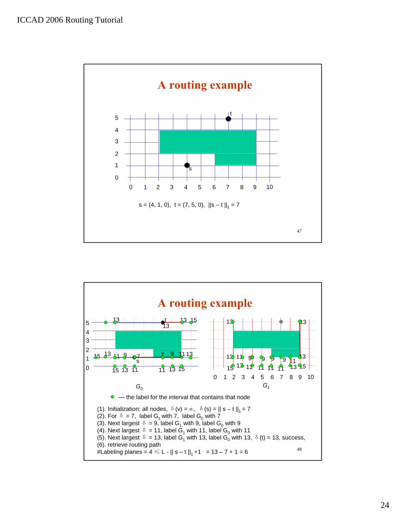
A routing example
s
t
0 1 2 4 5 6 7 8 9 1030
5
4
2
3
1
s = (4, 1, 0), t = (7, 5, 0), ||s – t ||1 = 7
48
A routing example
s
t
0
54
23
1
0 1 2 4 5 6 7 8 9 103G0
G1
(1). Initialization: all nodes, δ(v) = ∞, δ(s) = || s – t ||1 = 7 (2). For δ = 7, label G1 with 7, label G0 with 7(3). Next largest δ = 9, label G1 with 9, label G0 with 9(4). Next largest δ = 11, label G1 with 11, label G0 with 11(5). Next largest δ = 13, label G1 with 13, label G0 with 13, δ(t) = 13, success, (6). retrieve routing path #Labeling planes = 4 ≤ L - || s – t ||1 +1 = 13 – 7 + 1 = 6
13
7 9 99979 9
11 11 11 11
11 11 11111313
— the label for the interval that contains that node
11 11 1313
15
1515
151313
1515
1313
1313 1313

ICCAD 2006 Routing Tutorial
25
49
A routing example
s
t
0 1 2 4 5 6 7 8 9 1030
5
4
2
3
1
•Theoretically fast for simple paths with a small detour•Guarantees optimality
50
Gridless Detailed Routing
• Gridless Routing– More flexible
– Longer runtime due to complex data structure• Gridless Detailed Routing Algorithms
– Shape (Tile) based routing [Sato, et al., ISCS87, Margarino, et al., TCAD87, Dion, et al., WRL Research Report 95/3, Liu, et al., ISPD98]
– Graph-based routing [Wu, et al., TC87, Ohtsuki, ICCAS85, Cong, et al., Zheng, et al., TCAD96, ICCAD’99]
– Subgrid routing [US Patent, 6,507,941 B1, Jan. 2003]

ICCAD 2006 Routing Tutorial
26
51
Basic Operation: Obstacle Expansion in Gridless Routing
• In order to route a wire with width w and spacing sp– Obstacles are expanded
by w/2 + sp
• Reduced the problem to finding a zero-width routing path– [Schiele, et al., DAC 90] – [Dion, et al., WRL
Research Report 95/3] – [Cong, et al., ICCAD99]
S
T
52
DUNE [Cong, et al., ICCAD’99]
• Gridless routing engine [Cong, et al., ICCAD’99]– Non-uniform grid
graph– Implicit grid graph– Path-based Maze
SearchingS
T
y1y2
y3
y4y5y6
y7
y8

ICCAD 2006 Routing Tutorial
27
53
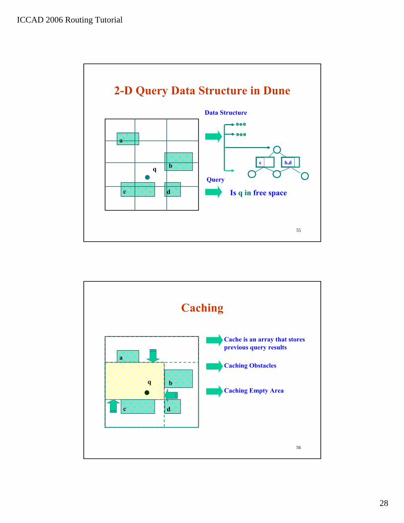
Rectangle-based Query• Given a set of rectangles and a query point q• Query: if the query point is contained by any of the
given rectangles
a
b
dc
q
54
Rectangle-based Query Algorithms
• K-D tree• Quad-list quad tree• Multiple storage quad tree• HV/VH tree• 1-D and 2-D indexing
ICCAD 2006 Routing Tutorial
28
55
2-D Query Data Structure in Dune
a
b
dc
q
Data Structure
Is q in free space
Query
c b,d
56
Caching
a
b
dc
q
Cache is an array that storesprevious query results
Caching Obstacles
Caching Empty Area
ICCAD 2006 Routing Tutorial
29
57
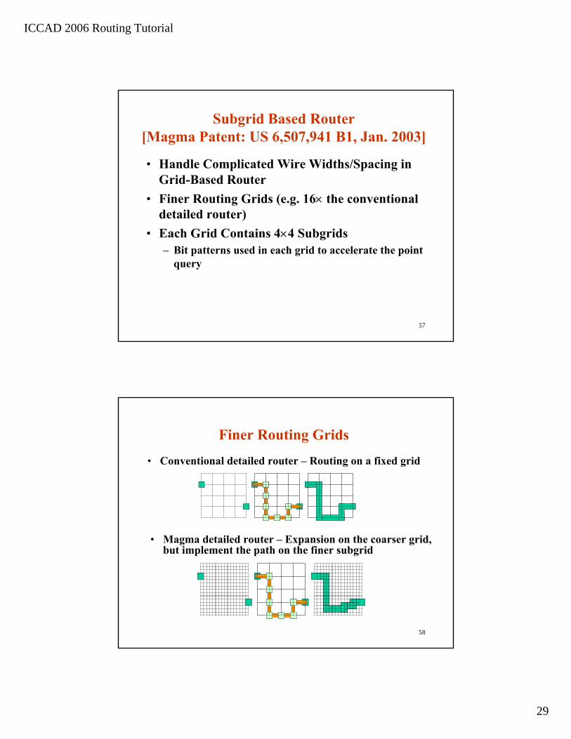
Subgrid Based Router [Magma Patent: US 6,507,941 B1, Jan. 2003]
• Handle Complicated Wire Widths/Spacing in Grid-Based Router
• Finer Routing Grids (e.g. 16× the conventional detailed router)
• Each Grid Contains 4×4 Subgrids– Bit patterns used in each grid to accelerate the point
query
58
Finer Routing Grids
• Conventional detailed router – Routing on a fixed grid
• Magma detailed router – Expansion on the coarser grid, but implement the path on the finer subgrid

ICCAD 2006 Routing Tutorial
30
59
Step 1: Build Subgrid Map• Expand obstacles by proper width and spacing• Covering subgrid points by expanded Obstacles (e.g. 14I, 14J, 14K)
1111111111111111
1111111111111111
1111111111111111
1111111111111111
1111111111111111
1111111111111111
1111111111110000
1111111111110011
0000000000000000
0011001100110011
1111111111111111
1111111111111111
0000000011110000
0000000011110011
0000000000000000
0011001100110011
1111111111111111
0111011111111111
0000000011110000
0000000011100010
0000000000000000
0010001100110011
0000111111111111
0000000000000000
14I
14I 14I
14J14J
14K
60
Step 2: Make Every Grid Map Reachable
• A grid map is reachable: iff every subgrid with “1” can be reached by other subgrid with “1”s
• Dropping some “1”s might be necessary
Reachable bit patterns
ICCAD 2006 Routing Tutorial
31
61
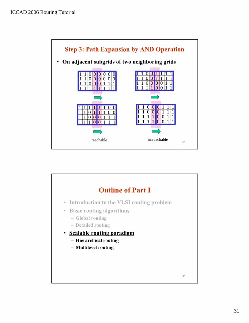
Step 3: Path Expansion by AND Operation
• On adjacent subgrids of two neighboring grids
0100000
111111111
1110000
111100000
0100000
111111111
1111111
100001111
0001011
111111111
1110000
110101111
1110000
111111111
1111111
100001010
reachable unreachable
62
Outline of Part I• Introduction to the VLSI routing problem• Basic routing algorithms
– Global routing– Detailed routing
• Scalable routing paradigm– Hierarchical routing– Multilevel routing
ICCAD 2006 Routing Tutorial
32
63
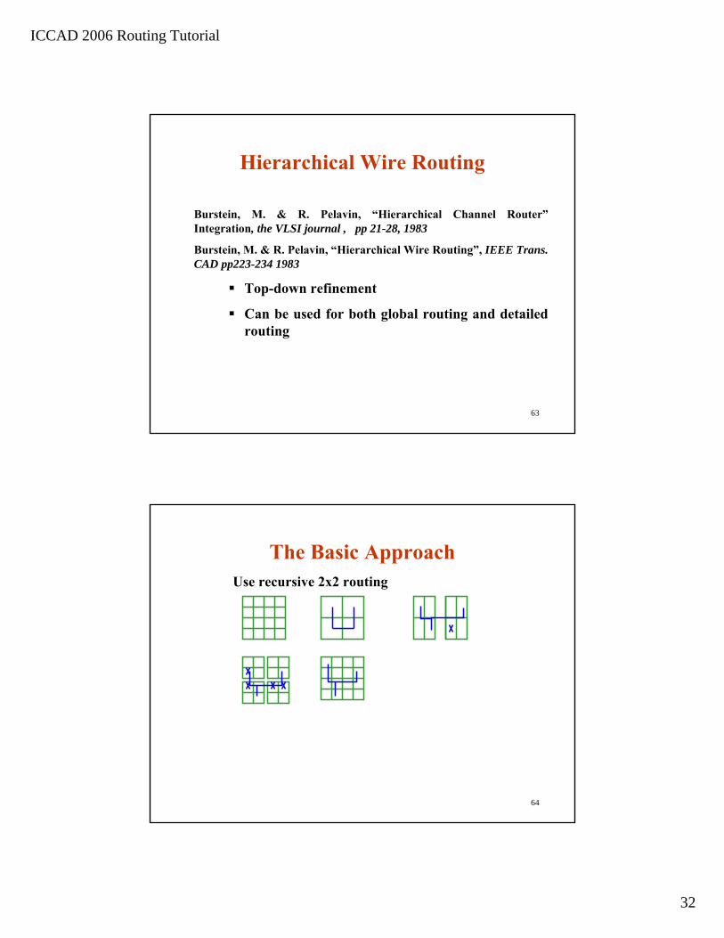
Hierarchical Wire Routing
Burstein, M. & R. Pelavin, “Hierarchical Channel Router”Integration, the VLSI journal , pp 21-28, 1983
Burstein, M. & R. Pelavin, “Hierarchical Wire Routing”, IEEE Trans. CAD pp223-234 1983
Top-down refinement
Can be used for both global routing and detailed routing
64
The Basic ApproachUse recursive 2x2 routing
ICCAD 2006 Routing Tutorial
33
65
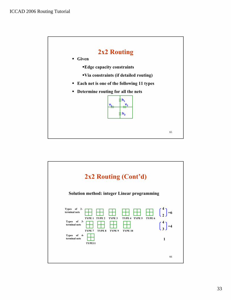
2x2 RoutingGiven
Edge capacity constraints
Via constraints (if detailed routing)
Each net is one of the following 11 types
Determine routing for all the nets
h1
h2
v1 v2
66
Types of 2-terminal nets
TYPE 1 TYPE 2 TYPE 3 TYPE 6TYPE 5TYPE 4
TYPE11
Types of 3-terminal nets
TYPE 7 TYPE 8 TYPE 9 TYPE 10
4
3=4
4
2=6
1Types of 4-terminal nets
2x2 Routing (Cont’d)
Solution method: integer Linear programming

ICCAD 2006 Routing Tutorial
34
67
Routing Configuration of Each Type of Nets
x(1,1), x(1,2)
x(2,1), x(2,2)
68
Routing Configuration of Each Type of Nets(Cont’d)
X(7,1), x(7,2), x(7,3)
x(11,1), x(11,2), x(11,3), x(11,4)
ICCAD 2006 Routing Tutorial
35
69
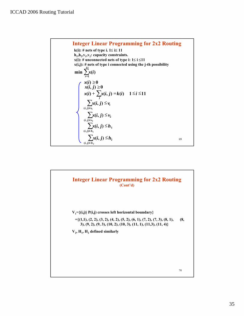
Integer Linear Programming for 2x2 Routingk(i): # nets of type i. 1≤ i≤ 11h1,h2,v1,v2: capacity constraints.x(i): # unconnected nets of type i: 1≤ i ≤11x(i,j): # nets of type i connected using the j-th possibility
∑
∑∑
∑∑
∑
∈
∈
∈
∈
=
≤
≤
≤
≤
≤≤=+≥
≥
2
1
2
1
),(2
),(1
),(2
),(1
11
1
),(
),(
),(
),(
111)(),()(0),(
0)(
)(min
hji
hji
vji
vji
j
r
hjix
hjix
vjix
vjix
iikjixixjix
ix
ix
70
Integer Linear Programming for 2x2 Routing(Cont’d)
V1={(i,j)| P(i,j) crosses left horizontal boundary}
={(1,1), (2, 2), (3, 2), (4, 2), (5, 2), (6, 1), (7, 2), (7, 3), (8, 1), (8, 3), (9, 2), (9, 3), (10, 2), (10, 3), (11, 1), (11,3), (11, 4)}
V2, H1, H2 defined similarly

ICCAD 2006 Routing Tutorial
36
71
ILP Approach for 2x2 Routing (Cont’d)
39 variables
15 linear equation
11 x(i)
28 x(i,j)= k(i) 11
≤ h1, h2, v1, v2 4
(19 equations, if we consider via constraints since we have 4 more equations for each super cell)
Can be solved efficiently
Map a net to a routing configuration using heuristic ( we only know the number of nets for each configuration)
72
Multilevel Routing Framework (MARS [TCAD05])
Fine routing tile generation Detailed routing
G1
Coarsening
G0
Refinement
Initial routing
Gk
G0
G1
•Multicommodity flow based algorithm
•History-based iterative refinement
•Implicit graph gridless routing
ICCAD 2006 Routing Tutorial
37
73
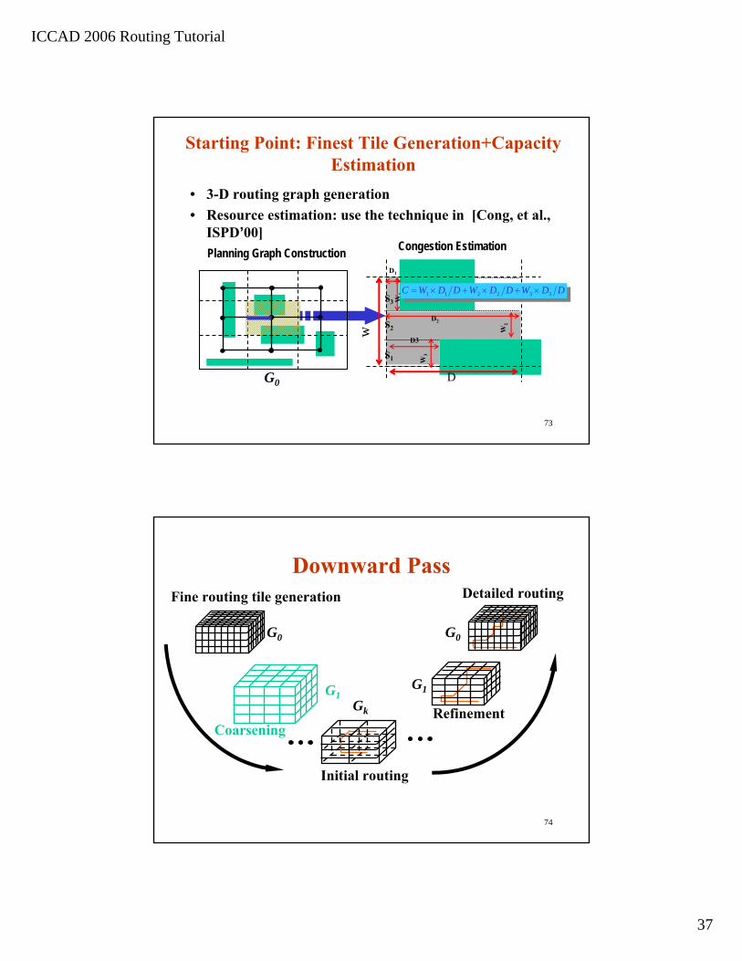
Starting Point: Finest Tile Generation+Capacity Estimation
• 3-D routing graph generation• Resource estimation: use the technique in [Cong, et al.,
ISPD’00]Planning Graph Construction Congestion Estimation
S1
S2
S3
wD
D2
D1
D3
W1
W3
W2
DDWDDWDDWC 332211 ×+×+×=
G0
74
Downward PassFine routing tile generation Detailed routing
G0
Refinement
Initial routing
Gk
G0
G1G1
Coarsening
ICCAD 2006 Routing Tutorial
38
75
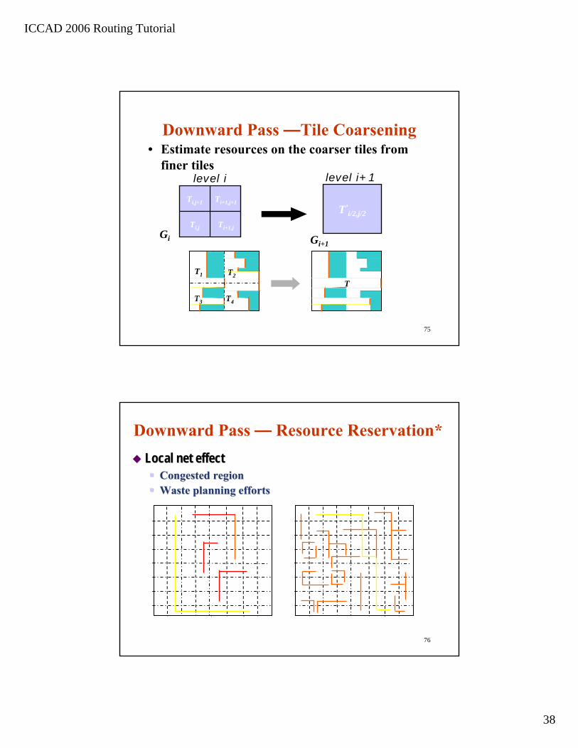
Downward Pass —Tile Coarsening• Estimate resources on the coarser tiles from
finer tiles
Ti,j
Ti,j+1 Ti+1,j+1
Ti+1,jGi Gi+1
T’i/2,j/2
level i level i+1
T1 T2
T3 T4
T
76
Downward Pass — Resource Reservation* Local net effectLocal net effect
Congested region Congested region Waste planning effortsWaste planning efforts

ICCAD 2006 Routing Tutorial
39
77
Initial Routing at Coarsest LevelFine routing tile generation Detailed routing
G1
Coarsening
G0
Refinement
Initial routing
Gk
G0
G1
78
Multicommodity Flow-Based Initial Routing
• Start the Planning at the Coarsest Level• Advantages of Multicommodity Flow-based
Algorithm– Fast enough for coarse grids– More global view, proved error bound to optimal for
fractional routing– Can be integrated with performance optimization by
including high-performance topologies, such as A-Tree, BA-Tree, and P-Tree
• Implemented the Algorithm in [Albrecht, ISPD’00]– Minimize the overall congestion– Randomized rounding
ICCAD 2006 Routing Tutorial
40
79
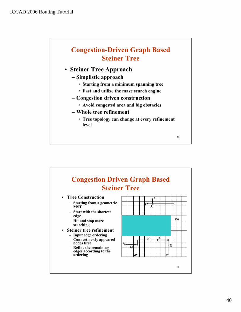
Congestion-Driven Graph Based Steiner Tree
• Steiner Tree Approach– Simplistic approach
• Starting from a minimum spanning tree• Fast and utilize the maze search engine
– Congestion driven construction• Avoid congested area and big obstacles
– Whole tree refinement• Tree topology can change at every refinement
level
80
c
ba
Congestion Driven Graph Based Steiner Tree
(2)
• Tree Construction– Starting from a geometric
MST– Start with the shortest
edge– Hit and stop maze
searching• Steiner tree refinement
– Input edge ordering– Connect newly appeared
nodes first– Refine the remaining
edges according to the ordering
(1)ba
c
d e
(2) (3)
(4)
(1)(1)
b
a
d
c
f
e
(1)
(3)
(4)
(2)
(5)
ICCAD 2006 Routing Tutorial
41
81
RefinementFine routing tile generation Detailed routing
G1
Coarsening
G0
Initial routing
Gk
G0
Refinement
G1
82
Incremental Refinement• Refine the coarser level results at the finer level
L1 L2
Local nets
N1
N2
N3
Global nets
preferred region for N3
• Use A* algorithm to find the path for each net
Routing graph for N3
Lower cost
Higher cost
ICCAD 2006 Routing Tutorial
42
83
History-Based Iterative Refinement
• History Based Multi-Iteration Refinement – First proposed in [Nair, TCAD’87 ], later used in
PathFinder [McMurchie et al, FPGA Symp’95]– Iteratively update each edge’s cost with the
consideration of historical congestion information – Reroute all the nets based on the new edge cost
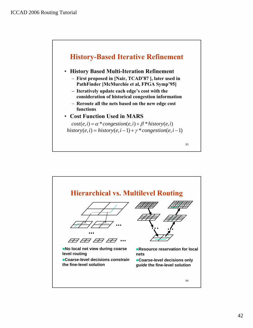
functions • Cost Function Used in MARS
( , ) * ( , ) * ( , )cost e i congestion e i history e iα β= +( , ) ( , 1) * ( , 1)history e i history e i congestion e iγ= − + −
84
Hierarchical vs. Multilevel Routing
No local net view during coarse level routing
Coarse-level decisions constrain the fine-level solution
Resource reservation for local nets
Coarse-level decisions only guide the fine-level solution
ICCAD 2006 Routing Tutorial
43
Part IIChallenges and Solutions to Large-Scale
IC Routing in Nanometer Designs
Tong Gao
86
Outline of Part II
• Objectives and new challenges for industrial routers
• Techniques for run time challenges• Techniques for capacity challenges• Techniques for design rules challenges• Techniques for DFM/DFY challenges
ICCAD 2006 Routing Tutorial
44
87
Objectives
• Traditional objectives– QoR – Via count, wire length, DRCs, and timing/crosstalk
• Via count and wire length cause congestion and affect yield• DRCs increase tapeout time, and possibly chip cost• Timing/crosstalk affects performance and post routing
optimization efforts– Run time
• Always one of the most important objectives• Closely related to QoR
– Memory• Very important for 32bit machines• Still important for 64bit machines
– Hardware is expensive– May lead to more run time
88
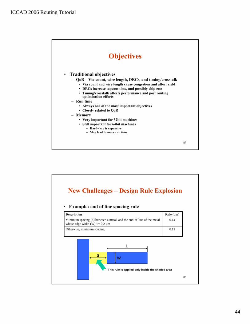
New Challenges – Design Rule Explosion
• Example: end of line spacing rule
0.11Otherwise, minimum spacing
0.14Minimum spacing (S) between a metal and the end-of-line of the metal whose edge width (W) <= 0.2 µm
Rule (µm)Description
W
L
S
This rule is applied only inside the shaded area
ICCAD 2006 Routing Tutorial
45
89
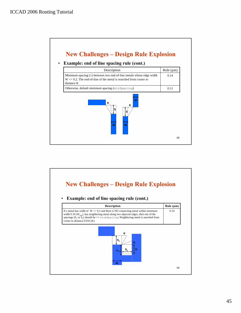
New Challenges – Design Rule Explosion• Example: end of line spacing rule (cont.)
0.11Otherwise, default minimum spacing (minSpacing)
0.14Minimum spacing (S) between two end-of-line metals whose edge width W <= 0.2. The end-of-line of the metal is searched from corner to distance K
Rule (µm)Description
W
S
W
K
W
S
K
90
New Challenges – Design Rule Explosion
• Example: end of line spacing rule (cont.)
0.14If a metal has width of W <= 0.2 and there is NO connecting metal within minimum width 0.16 (Wmin), has neighboring metal along two adjacent edges, then one of the spacings (S1 or S2) should be >= stubSpacing; Neighboring metal is searched from corner to distance 0.035 (K)
Rule (µm)Description
S1
S2 S
W
K
K
Wmin

ICCAD 2006 Routing Tutorial
46
91
New Challenges – Design Rule Explosion
• Example: end of line spacing rule (cont.)
0.14If a metal of width (W) <= 0.2 has neighboring metals along three adjacent edges, then one of the spacings (S1 or S2 or S3) should be >= 0.14
Rule (µm)Description
S
S2W
S1
S
92
New Challenges – Design Rule Explosion
• Example: end of line spacing rule (cont.)– Progressively becomes more complicated
• Need to support each intermediate form
– Spacing rules involves a lot more than 2 shapes• Analysis challenge – multiple neighbors with pattern• DRC book keeping challenge – no more two shape DRCs • Optimization challenges – many alternatives to resolve
DRCs, and many new ways to create to DRCs
– Benefit from polygon• Routing is rectangle based
ICCAD 2006 Routing Tutorial
47
93
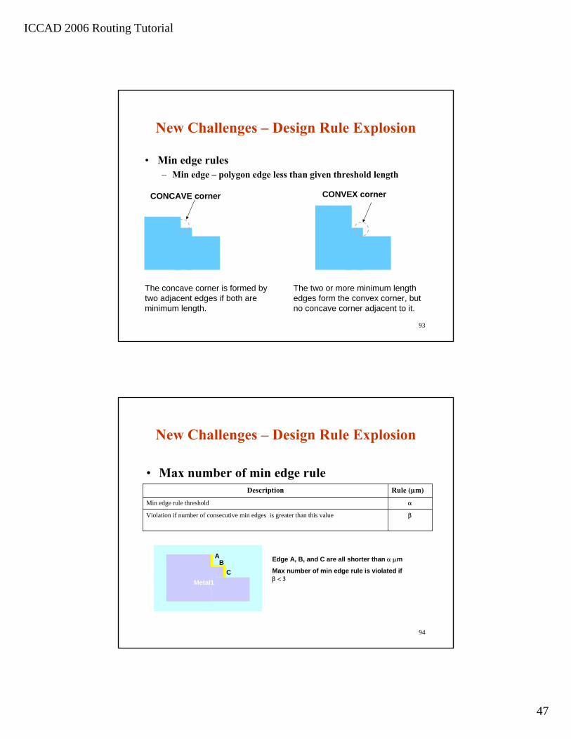
New Challenges – Design Rule Explosion
• Min edge rules– Min edge – polygon edge less than given threshold length
CONVEX corner
The two or more minimum length edges form the convex corner, but no concave corner adjacent to it.
CONCAVE corner
The concave corner is formed by two adjacent edges if both are minimum length.
94
New Challenges – Design Rule Explosion
• Max number of min edge rule
αMin edge rule threshold
βViolation if number of consecutive min edges is greater than this value
Rule (µm)Description
Edge A, B, and C are all shorter than α µm
Max number of min edge rule is violated if β < 3
AB
CMetal1

ICCAD 2006 Routing Tutorial
48
95
New Challenges – Design Rule Explosion
• Total min edge length rules
αIf there is at least one edge less than the minimum edge length,
βViolation if the sum of the minimum edge lengths is greater than this value
Rule (µm)Description
Edge A, B, and C are all shorter than α µm
Total minimum edge length rule is violated if length of (A + B + C) > β µm
AB
CMetal1
96
New Challenges – Design Rule Explosion
• Min edge length rules– If minEdgeMode = 0, a concave corner is needed
AB
C
A, B, C < α and A + B + C > β
Total minimum edge length rule is violated
Concave Corner BC
Convex Corner
B, C < α and B + C > β
Total minimum edge length rule is not violated
Metal1 Metal1
minEdgeMode = 0 minEdgeMode = 0

ICCAD 2006 Routing Tutorial
49
97
New Challenges – Design Rule Explosion
• Min edge length rules (cont.)– If minEdgeMode = 1, a concave corner is not needed
A, B, C < α and A + B + C > β
Total minimum edge length rule isviolated
B, C < α and B + C > β
Total minimum edge length rule isviolated
AB
C BC
Convex Corner
Metal1 Metal1
Concave Corner
minEdgeMode = 1 minEdgeMode = 1
98
New Challenges – Design Rule Explosion
• Min edge rule– Analysis challenge – Totally polygon based while
routing shapes are rectangles– DRC book keeping challenge – for multiple shapes
along edges– Optimization challenges – many different ways to
fix the DRCs• Patching• Shifting• Via rotating• Rerouting
ICCAD 2006 Routing Tutorial
50
99
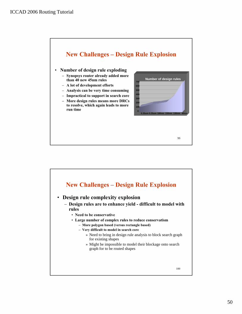
New Challenges – Design Rule Explosion
• Number of design rule exploding– Synopsys router already added more
than 40 new 45nm rules– A lot of development efforts– Analysis can be very time consuming– Impractical to support in search core – More design rules means more DRCs
to resolve, which again leads to more run time
Number of design rules per process node
0
100
200
300
400
500
600
700
0.35um 0.25um 180nm 150nm 130nm 90nm
100
New Challenges – Design Rule Explosion
• Design rule complexity explosion– Design rules are to enhance yield - difficult to model with
rules• Need to be conservative• Large number of complex rules to reduce conservatism
– More polygon based (versus rectangle based)– Very difficult to model in search core
» Need to bring in design rule analysis to block search graph for existing shapes
» Might be impossible to model their blockage onto search graph for to be routed shapes
ICCAD 2006 Routing Tutorial
51
101
New Objectives – Design Rules
• Design rule number and complexity, and large design size compound with each other, causing major implementation, quality, runtime, and memory challenges
• New objective: have the ability to add large number of new complex design rules in short period of time, while keeping run time/memory under control
102
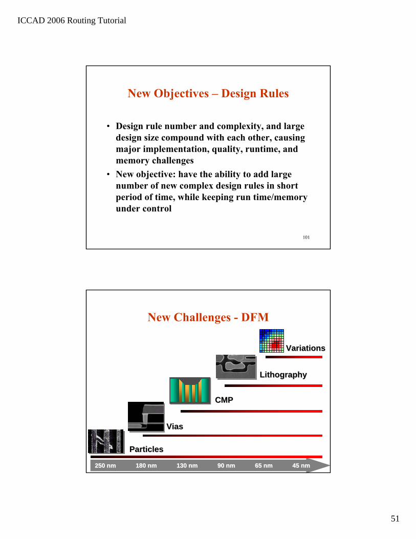
New Challenges - DFM
250 nm250 nm 180 nm180 nm 130 nm130 nm 90 nm90 nm 65 nm65 nm 45 nm45 nm
ParticlesParticles
ViasVias
LithographyLithography
CMPCMP
VariationsVariations
ICCAD 2006 Routing Tutorial
52
103
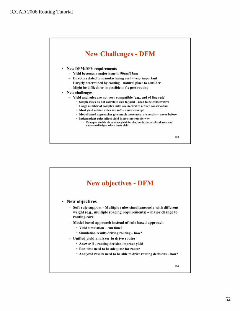
New Challenges - DFM
• New DFM/DFY requirements– Yield becomes a major issue in 90nm/65nm– Directly related to manufacturing cost – very important– Largely determined by routing – natural place to consider– Might be difficult or impossible to fix post routing
• New challenges– Yield and rules are not very compatible (e.g., end of line rule)
• Simple rules do not correlate well to yield – need to be conservative• Large number of complex rules are needed to reduce conservatism• Most yield related rules are soft – a new concept• Model based approaches give much more accurate results – never before• Independent rules affect yield in non-monotonic way
– Example, double via enhance yield for vias, but increase critical area, and cause small edges, which hurts yield
104
New objectives - DFM
• New objectives– Soft rule support - Multiple rules simultaneously with different
weight (e.g., multiple spacing requirements) – major change to routing core
– Model based approach instead of rule based approach• Yield simulation – run time?• Simulation results driving routing – how?
– Unified yield analyzer to drive router• Answer if a routing decision improve yield• Run time need to be adequate for router• Analyzed results need to be able to drive routing decisions – how?
ICCAD 2006 Routing Tutorial
53
105
Outline of Part II
• Objectives and new challenges for industrial routers
• Techniques for run time challenges• Techniques for capacity challenges• Techniques for design rules challenges• Techniques for DFM/DFY challenges
106
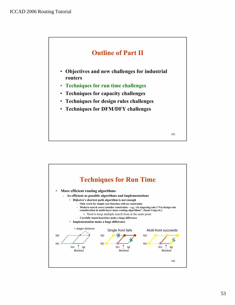
Techniques for Run Time• More efficient routing algorithms
– As efficient as possible algorithms and implementations• Dijkstra’s shortest path algorithm is not enough
– Only work for simple cost function with no constraints– Modern search cores consider constraints – e.g., via stagering rule (“Via design rule
consideration in multi-layer maze routing algorithms”, Jason Cong etc.)» Need to keep multiple search front at the same point
– Carefully tuned heuristics make a huge difference• Implementation make a huge difference
Src tgtM1
M2
BlockedSrc tgt
M1
M2
Blocked
< stager distance Single front fails
Src tgtM1
M2
Blocked
Multi-front succeeds

ICCAD 2006 Routing Tutorial
54
107
Techniques for Run Time
• More efficient routing algorithms (cont.)– Stay away from more time consuming algorithms
• Shape based, gridless routers• Can achieve gridless routing effect with gridded router
– Gridless routing cause space fragmentation, not good for early iterations
– Can achieve gridless effects by using finer grids – good enough in practice
108
Techniques for Run Time
• More efficient routing algorithms (cont.)– Search cores support few basic rules
• Incorporating new rules directly into search core will kill the run time• Keep new complex design rules out of search core
– More later• Only keep most commonly supported rules in search core
– Spacing between different nets– Staggering distance– Antenna layer hopping– …
– DRC convergence has a huge effect on run time• Multiple iteration DRC convergence• Run time is determined by how fast DRC converge
– Resolving DRC too fast cause longer wires, more vias, and entangled routes» Bad quality and longer run time
– Resolving DRC too slow leads to many iterations – longer run time– It is an art to balance the speed of DRC convergence
ICCAD 2006 Routing Tutorial
55
109
Techniques for Run Time
• Hierarchical routing – break up the complexity– More routing stages – global routing/track
assign/detailed routing– Hierarchical global routing– Multilevel routing– Partition/corridor based iterative routing
110
Techniques for Run time
• Take advantage of the latest hardware development– Linux multi-processor computer farms are
everywhere• Multithreading for multi-processor machines• Distributed computing for computer farm• Combined for both

ICCAD 2006 Routing Tutorial
56
111
Techniques for Run Time
• Threading versus distributed computing
Expensive, difficultCheap, easyProc comm. cost
Larger, non-interacting,slow changing subtasks
Smaller, interacting, fast changing subtasks
Parallel style
Very expensiveCheapNew proc cost
LittleVery highRetrofit difficulty
LessMore, but for better programming
New router difficulty
No requirementModular, cleanData structure req.
Less subtask memMore work memMemory usage
MoreFewer# avail proc
Dist. Comp.Threading
112
Techniques for Run Time
• Multithreading– Hardware readiness
• Dual-core processors are common nowadays• Multi-processor machines are common also
– 2 – 4 processor machines are cheap main stream machines
– Offers significant scalable speedup with relatively low efforts
• Much easier to obtain scalable speedup compared to algorithm improvement
ICCAD 2006 Routing Tutorial
57
113
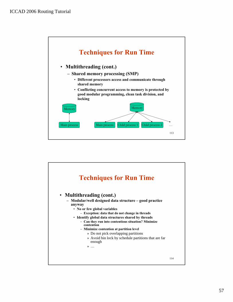
Techniques for Run Time
• Multithreading (cont.)– Shared memory processing (SMP)
• Different processors access and communicate through shared memory
• Conflicting concurrent access to memory is protected by good modular programming, clean task division, and locking
Main process
Memory
Main process
Memory
Child process 1 Child process 2 …
114
Techniques for Run Time
• Multithreading (cont.)– Modular/well designed data structure – good practice
anyway• No or few global variables
– Exception: data that do not change in threads• Identify global data structures shared by threads
– Can they run into contentious situation? Minimize contention
– Minimize contention at partition level» Do not pick overlapping partitions» Avoid bin lock by schedule partitions that are far
enough» …

ICCAD 2006 Routing Tutorial
58
115
Techniques for Run Time
• Multithreading (cont.)– Modular data
• Group data to minimize contentious data structures– Separate contentious data from non-contentious data in global data
structure– Choose thread specific data structure over global data structure
– Different levels of data caching to reduce dependency on global data
• Two tie data – global persistent data and thread specific working data (DRC)
– Thread specific data is checked out at beginning, and checked in at the end
– Great for memory usage also– Example - DRCs
116
Techniques for Run Time
• Multithreading (cont.)– Contention prevention – partition to break interactions
• Routing is partition based – design rules are mostly area based• Pick non-adjacent partitions to multithread
– No area conflicts, less other conflicts– Still desirable to expand out continuous partition front for uniform
partitions – less misalignments • Break shapes across partitions, or avoid partitions sharing shapes

ICCAD 2006 Routing Tutorial
59
117
Techniques for Run Time
• Multithreading (cont.)– Contention prevention – lock design
• Design data structures to minimize lock needed for frequently accessed data
• Balance between run time, memory, complexity– Place lock at the lower level to minimize contention, at the cost of
run time, memory, and more complicated control– Place lock at the higher level to trade off above– Example – global binning structure for geometry query
Top level lock Bin level lock Sub-bin level lock
118
Techniques for Run Time
• Multithreading (cont.)– Use scheduler to reduce waiting for lock
• Example: need net lock for antenna– Use a round robin scheduler in each thread to schedule nets– Reduce the amount of lock due to different threads working
on the same net
No scheduler
Scheduler
A B C
D B E
Thread 1
Thread 2
A B C
D B E
A B C
D B E
B C
B E
B C
BE
C
B E
C
B
E

ICCAD 2006 Routing Tutorial
60
119
Techniques for Run Time
• Multithreading (cont.)• Non-determinism
– Unless tasks are totally independent, will have non-determinism
» Could be challenging for debugging» Will not always produce the same results, but should
produce similar results– Reduce non-determinism
» No hash on pointer» Thread specific random number generator» Use algorithms that are as order independent as
possible» …
120
Techniques for Run Time
• Distributed computing– Divide routing problems into (almost independent) multiple
subtasks, and send the subtasks to different processes on different processors and/or machines with minimum communication
– Has more processors available– Subtask overhead is high – smaller number of larger subtasks– Subtasks need to be as independent as possible
• Communication between processes is difficult and expensive• Certain rules such as antenna rule is not localized, therefore
difficult with distributed computing– As a result, the scalability and quality using distributed
computing is usually not as good as for multithreading

ICCAD 2006 Routing Tutorial
61
121
Outline of Part II
• Objectives and new challenges for industrial routers
• Techniques for run time challenges• Techniques for capacity challenges• Techniques for design rules challenges• Techniques for DFM/DFY challenges
122
Techniques for Capacity
• Better infrastructure design– Think of memory as your own money – be stingy– Go after every bit in highly repeated data structures– Use bit fields

ICCAD 2006 Routing Tutorial
62
123
Techniques for Capacity• Two tiered in memory data storage
– Store non-derivable persistent data in as lean form as possible – e.g., use center line to represent routing shapes
– Derive partition level data in more run time friendly ways –e.g., fully instantiate routing related shape information
– Best balance between data size and run time
M1 wire
M2 w
ire
M1M2 via(x1, y1, lay1, widIdx1)
(x2, lay2, widIdx2)
(y2, lay3, widIdx3)
Total: 7 words
Abstract representationDetailed representation
M1/M2 wire: x1, y1, x2, y2, layer
Low surround/cut/high surround: x1, y1, x2, y2, layer
Total: 25 words
Routing
124
Techniques for Capacity
• Child process– Very useful to break 32bit 4G limit– Might still help memory caching for better speed for
64bit
• Distributed computing– Smaller distributed subtasks, which consume less
memory per subtasks
ICCAD 2006 Routing Tutorial
63
125
Outline of Part II
• Objectives and new challenges for industrial routers
• Techniques for run time challenges• Techniques for capacity challenges• Techniques for design rules challenges• Techniques for DFM/DFY challenges
126
Techniques for Design Rule• DRC analysis
– Trend - polygon based• Past rules are rectangular based
– Less complexity– No polygon generation time
• More and more rules are polygon based• Routing shapes are rectangles• Difficult and inefficient to convert polygon based rules to rectangle based
rules• Balance tipping towards polygon manipulations• Bite the bullet and maintain polygons along rectangles
AB
C
Metal1

ICCAD 2006 Routing Tutorial
64
127
Techniques for Design Rule
• DRC analysis (cont.)– DRC annotation
• Routing shapes are still rectangles• Need to map DRCs from polygon to relevant rectangles
AB
C
Metal1
128
Techniques for Design Rule
• Search core– Search graph (maze map): only blocked by basic spacing rules
• Heavy development needed if introduce new rules• Significant run time increase is expected for new rules• Very difficult if possible to block maze map for rules depending
on routing pattern of to be routed wires– Search core: only consider as few constraints as possible
besides maze map blockage• Very difficult to introduce new rules in the middle of search• Significant run time increase is expected for new rule• Changes will cause stability issues in routing core in continuous
way
ICCAD 2006 Routing Tutorial
65
129
Techniques for Design Rule
• Search core (cont)– Search core avoid resolve DRCs by avoiding DRC areas
• DRC areas are mapped into maze map• Extra cost are added for DRC areas during routing• Extra DRC cost decays with a carefully designed schedule
– Slow decay causes massive over blockage– Fast decay leads to DRC oscillation
• Advantages – scalable search core, no development, memory, and run time penalty for routing search, work well for less frequentDRCs
• Disadvantages – Requires more search and repair, expensive and does not work well for high frequency DRCs
130
Techniques for Design Rule
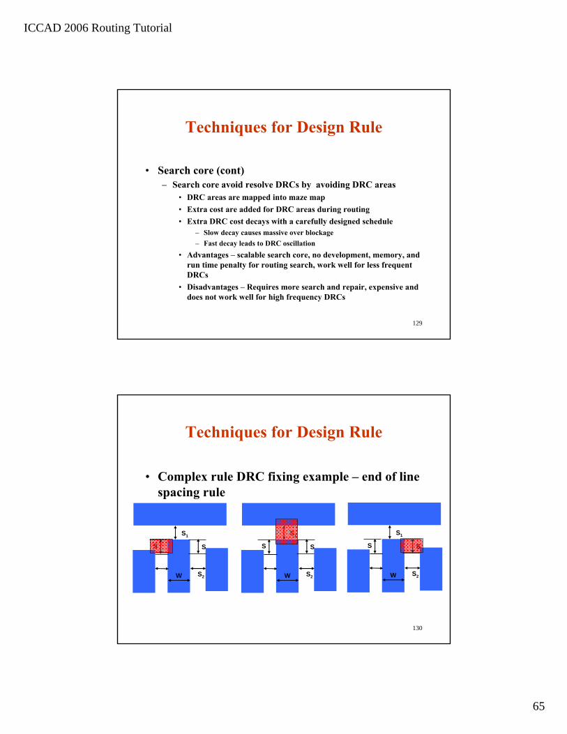
• Complex rule DRC fixing example – end of line spacing rule
S
S2W
S1
S S
S2W
S1
S S
S2W
S1
S
ICCAD 2006 Routing Tutorial
66
131
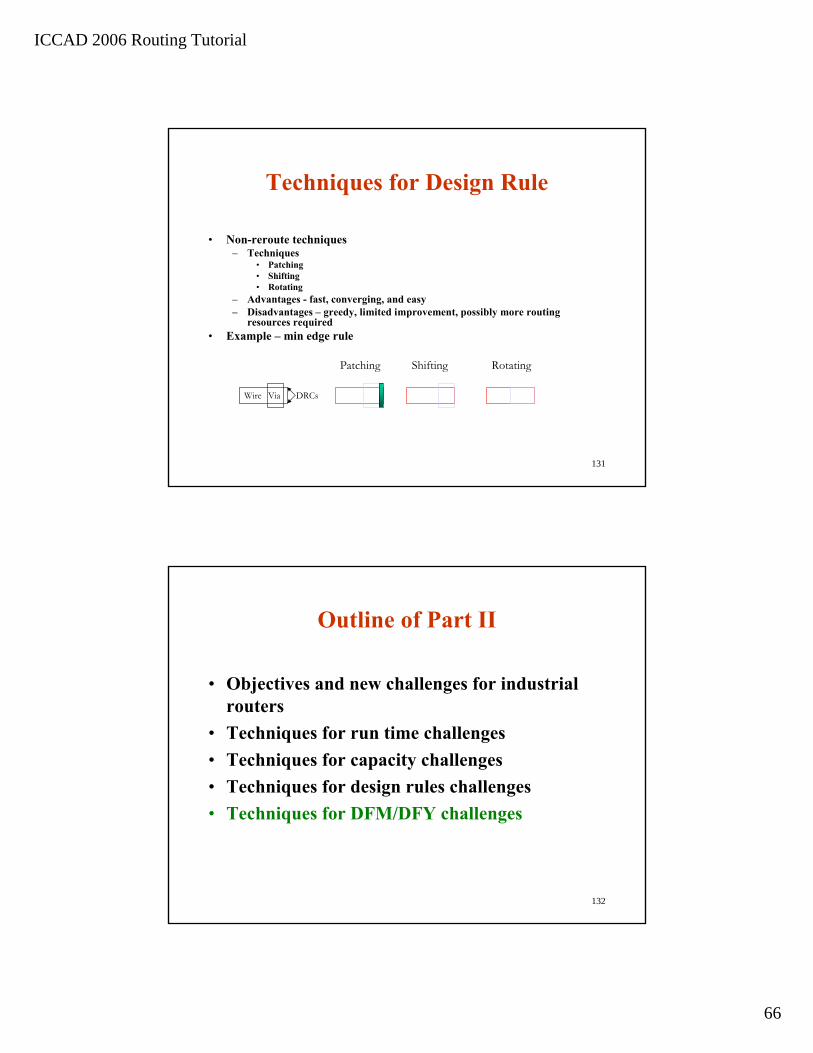
Techniques for Design Rule
• Non-reroute techniques– Techniques
• Patching• Shifting• Rotating
– Advantages - fast, converging, and easy– Disadvantages – greedy, limited improvement, possibly more routing
resources required • Example – min edge rule
Wire Via DRCs
Patching Shifting Rotating
132
Outline of Part II
• Objectives and new challenges for industrial routers
• Techniques for run time challenges• Techniques for capacity challenges• Techniques for design rules challenges• Techniques for DFM/DFY challenges

ICCAD 2006 Routing Tutorial
67
133
Techniques for DFM/DFY• CAA/wire spreading/wire widening
– Critical area - the region where, if the center of a random defect with certain size falls on, it will cause circuit failure(yield loss)
• A good metric for yield • Reduction of Critical Area increases defect-limited yield
Critical Area
Conductive Defect Causing Short Non-Conductive Defect Causing Open
134
Techniques for DFM/DFY
• CAA/wire spreading/wire widening (cont.)– Critical area (cont.)
• Critical area value varies with defect size– For a given layout, the larger the defect size, the larger the critical
area– Average critical area is usually used
∫∞
=0
)()(x crcr dxxfxAA
Acr: average critical areax0: smallest particle sizex: defect size (diameter)Acr(x): critical area for defect size xf(x): defect size distribution function

ICCAD 2006 Routing Tutorial
68
135
Techniques for DFM/DFY• CAA/wire spreading/wire widening (cont.)
– Current flow
Wire Spreading/widening
Design Ready for Signal Routing
Detail Route and S&R
Critical Area Analysis
Density-Driven Global Route
Density-Driven Track Assign
136
Techniques for DFM/DFY
• Density driven global routing – distribute unused space more evenly across design– Reduce congestion overflow threshold
• May cause significant wire/via increase – careful tuning• May interact with real routing congestion
– Non-constant/non-liner over-congestion cost– Reduce conservatism as iteration goes
– Better approach – have another congestion map for wire spreading
• Better separation of real congestion and wire spreading• Tune wire spreading congestion cost against real congestion cost
ICCAD 2006 Routing Tutorial
69
137
Techniques for DFM/DFY
• Post DR wire spreading– Sub-pitch tracks for more continuous wire
spreading– Ripup and reroute with bigger spacing
requirements• Better approach – wire spreading during
detailed routing with softer spacing rules on wires together with regular spacing– Up to this point, each wire has one spacing rule– No tool does this yet
138
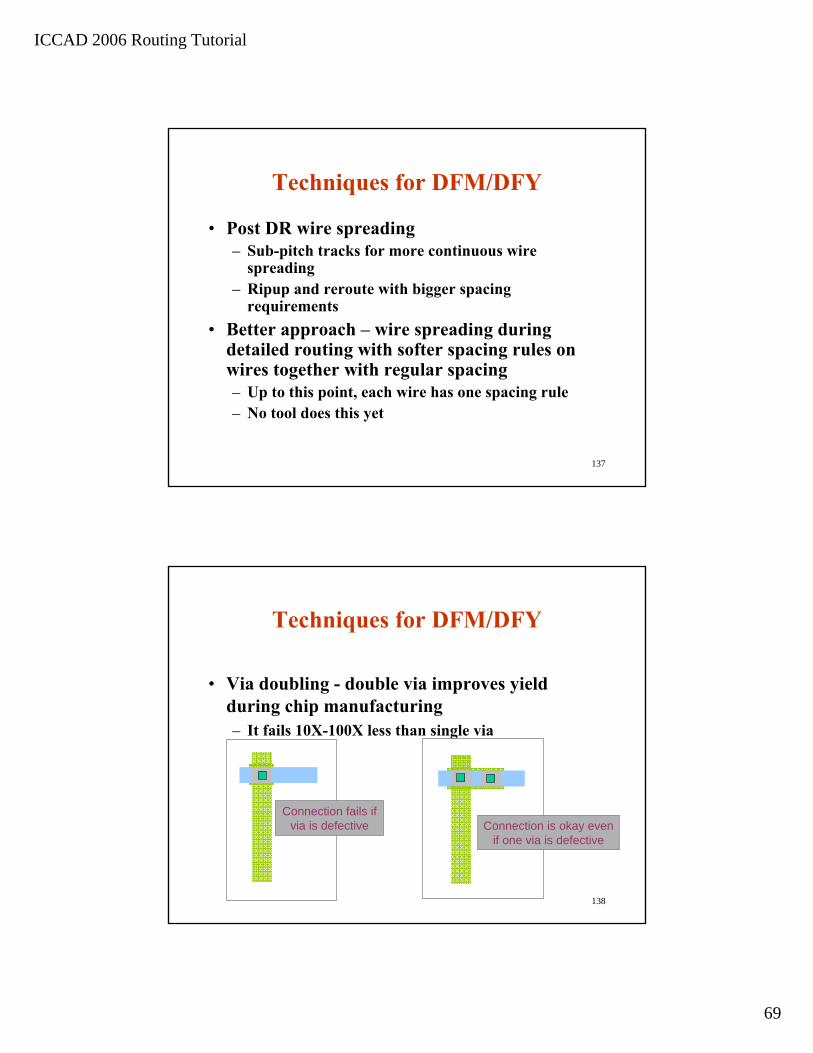
Techniques for DFM/DFY
• Via doubling - double via improves yield during chip manufacturing– It fails 10X-100X less than single via
Connection is okay even if one via is defective
Connection fails if via is defective

ICCAD 2006 Routing Tutorial
70
139
Techniques for DFM/DFY
• Via doubling– Rotates and swaps line via arrays to best fit into
available space
form into 1X2
swap into 2X1
rotate into 2X1
rotate into 1X2
single via
140
Techniques for DFM/DFY• Via doubling (cont.)
– Mostly done as a post routing process• Pros: Does not affect overall DRC convergence• Cons: limited by routing results, timing variance
– Newer approaches• Support soft spacing rules around vias to reserve space• Double via before post route timing closure, and keep doubling via
after timing optimizationBefore Via Optimization
(single vias)After Via Optimization
(double vias)

ICCAD 2006 Routing Tutorial
71
141
Techniques for DFM/DFY
• Litho aware routing– Many routing rules to
compensate for lack of simulation• Via proximity• Line-end• Length based
– Need to consider litho-effects w/o exploding routing rules
DRC - CleanDRC DRC -- CleanClean
Short on WaferShort on WaferShort on Wafer
142
Techniques for DFM/DFY
• Litho hot spot fixing– Run litho compliance check (LCC), identify hot
spots and replacement patterns– Replace with patterns suggested by LCC– Fix possible resulting DRCs

ICCAD 2006 Routing Tutorial
72
143
Techniques for DFM/DFY
Wide LineWide Spacing
Fine LineWide Spacing
Wide LineFine Spacing
Dishing
Erosion
Fine LineFine Spacing
Pattern dependent effects dictate a need for correct
type and amounts of metal fill
!!
144
Techniques for DFM/DFY• Metal fill
– Density driven metal fill is not good enough
Density Map Thickness Map
Same Density Different Thickness

ICCAD 2006 Routing Tutorial
73
145
Techniques for DFM/DFY• Model based CMP
– Driven by thickness simulation– Many patterns to choose from for least thickness variation
Rule-Based CMP-Aware Model-Based
Density Only Density and Thickness
Pattern selection based on simulation
146
Techniques for DFM/DFY
• Future works– New area in routing, a lot of on going projects– Need to have a unified yield analyzer and cost
function to drive optimization• Example
– via doubling improve yield– Critical area decrease yield– Complex geometries decrease yield– Is via doubling good for yield?
After Via Optimization(double vias)
ICCAD 2006 Routing Tutorial
©R.A. Rutenbar, 2006 1
© R.A. Rutenbar 2006
Part IIIAnalog and Mixed Signal Issues
Part IIIAnalog and Mixed Signal Issues
Rob A. RutenbarProfessor, Electrical & Computer Engineering
© R.A. Rutenbar 2006 Slide 2
And Now, For Something Completely Different…

ICCAD 2006 Routing Tutorial
©R.A. Rutenbar, 2006 2
© R.A. Rutenbar 2006 Slide 3
Why Analog Matters: Many “Mixed-Signal” SoCs
Mixed-Signal ChipsMixed-Signal ChipsTelecom Automotive
Computers& Networks
Consumer Medical
12%
30%
75%
2000 2003 2006
% Digital Chips withAnalog Content
%
[Source: IBS 2003]
© R.A. Rutenbar 2006 Slide 4
Routing in the Digital World: Summary
Capacity issues1-10 million placed instancesMillions of wires and pins
Nanometer issuesIncreasingly complex DRC rulesMore (and conflicting) DFM rules
Complexity issuesBillions of shapesCoupling, timing closure, yield and manufacturability iterationsDon’t want to spend CPU months
Problems look like thisIBM network switchIP blocks + N million gates
Courtesy Juergen Koehl, IBM

ICCAD 2006 Routing Tutorial
©R.A. Rutenbar, 2006 3
© R.A. Rutenbar 2006 Slide 5
Is Analog/Mixed-Signal Problem Basically Same?
Courtesy Frank Op’t Eynde, Alcatel
AnalogFrontendAnalog
FrontendAnalog
FrontendAnalog
Frontend
CPU CoreCPU CoreDSPDSP
MemoryMemory
Logic
Mem
Mem
Are we just routing a big set of analog
pins with a million min-width wires?
NO.
© R.A. Rutenbar 2006 Slide 6
Backing Up: What Exactly Gets Routed, Digital-Side?
Gates (standard cells) and IP blocks (memory, core, etc)Gates in rows, with large interspersed macro blocksWires over the top of everything (except a few very sensitive macros)
Soft IP:CPUCore
RandomLogic Hard IP: Memory, etc
More random logic
Cells
W iring
ICCAD 2006 Routing Tutorial
©R.A. Rutenbar, 2006 4
© R.A. Rutenbar 2006 Slide 7
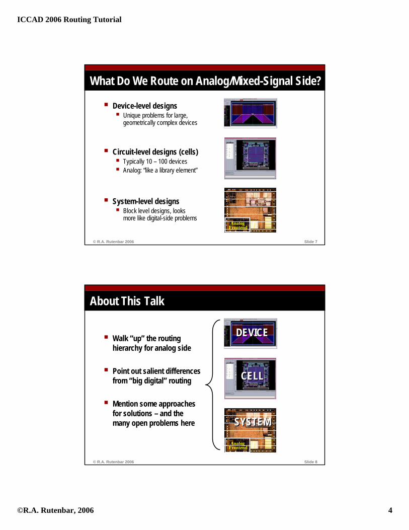
What Do We Route on Analog/Mixed-Signal Side?
Device-level designsUnique problems for large,geometrically complex devices
Circuit-level designs (cells)Typically 10 – 100 devicesAnalog: “like a library element”
System-level designsBlock level designs, looksmore like digital-side problems
AnalogFrontend
© R.A. Rutenbar 2006 Slide 8
About This Talk
Walk “up” the routinghierarchy for analog side
Point out salient differencesfrom “big digital” routing
Mention some approachesfor solutions – and themany open problems here
AnalogFrontend
DEVICEDEVICE
CELLCELL
SYSTEMSYSTEM

ICCAD 2006 Routing Tutorial
©R.A. Rutenbar, 2006 5
© R.A. Rutenbar 2006 Slide 9
Background: Low-Level Routing
First question: Why are we worrying about routing problems at theseseemingly “low” levelsof design hierarchy
Said differentlyIsn’t this what libraries are supposed to hide from system designers?
AnalogFrontend
DEVICEDEVICE
CELLCELL
SYSTEM
© R.A. Rutenbar 2006 Slide 10
Role of Digital Cells in Digital System Design
Digital ASIC design Usually starts from assumed library of cells (usually some cores too)Supports changes in cell-library; assumed part of methodologyCell libraries heavily reused across different designs
DigitalHDL
LogicSynthesis
TechMapping
PhysicalDesign
Gate-Level Cell Library
ICCAD 2006 Routing Tutorial
©R.A. Rutenbar, 2006 6
© R.A. Rutenbar 2006 Slide 11
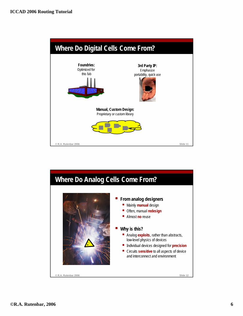
Where Do Digital Cells Come From?
Foundries:Optimized for
this fab
3rd Party IP:Emphasize
portability, quick use
Manual, Custom Design:Proprietary or custom library
© R.A. Rutenbar 2006 Slide 12
Where Do Analog Cells Come From?
From analog designersMainly manual design Often, manual redesignAlmost no reuse
Why is this?Analog exploits, rather than abstracts, low-level physics of devicesIndividual devices designed for precisionCircuits sensitive to all aspects of device and interconnect and environment
—+

ICCAD 2006 Routing Tutorial
©R.A. Rutenbar, 2006 7
© R.A. Rutenbar 2006 Slide 13
Why No Analog Libraries: DimensionalityProblem: many continuous specs for analog cells
Can’t just build a practical-size, universal analog libraryNote, people still do “library” some useful cells as hard IP (layouts), but still expect most cells you need will not be in your average library
−+ =
11/4 11/4
42/3 42/3
3/3 3/3
3/4 3/4
160/12
10pF
?10pF
In- In+ 23礎54礎 3/52
10 independentperformancespecifications
=
Spec=LOWSpec=HIGH
variantsfor ALL
combinations
X = ~ 1000 variantsfor just this cell
© R.A. Rutenbar 2006 Slide 14
About This Talk
Routing at device level
AnalogFrontend
DEVICEDEVICE
CELL
SYSTEM

ICCAD 2006 Routing Tutorial
©R.A. Rutenbar, 2006 8
© R.A. Rutenbar 2006 Slide 15
Device-Level Routing Issues
Focus is always on precisionWant precise electrical characteristics, or matching among several devices, or precise ratios among devices
Central issuesAnalog devices are often larger; e.g., a 4000/4 FET is not unusualAnalog devices are often designed and laid out as a careful connection of many small, well-matched unit-size devicesM-factors: 1 device M matched, inter-digitated devices/fingers in layoutGuard-ring(s) common for electrical isolation
ResultEven 1 device may end up with a complex, large geometric layout
© R.A. Rutenbar 2006 Slide 16
Example of Digital vs Analog Geometry DisparityDigital FET Analog FET
Device-levelrouting
ICCAD 2006 Routing Tutorial
©R.A. Rutenbar, 2006 9
© R.A. Rutenbar 2006 Slide 17
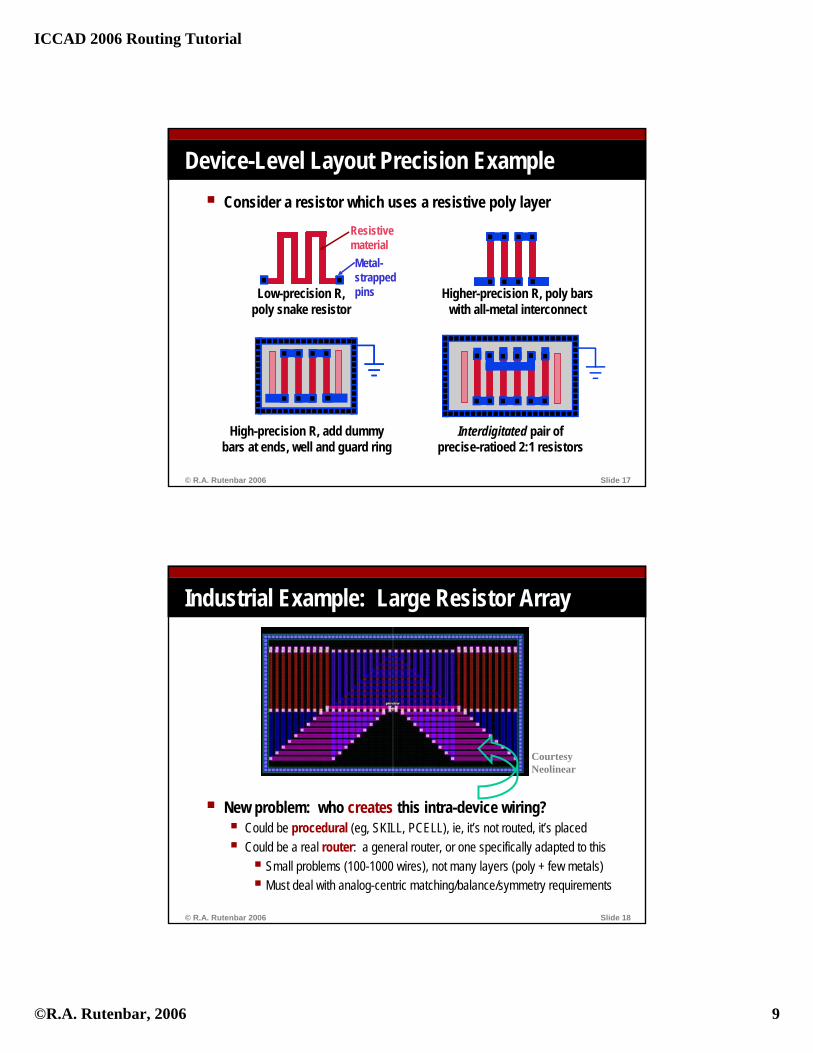
Device-Level Layout Precision ExampleConsider a resistor which uses a resistive poly layer
Low-precision R,poly snake resistor
Resistive materialMetal-strappedpins Higher-precision R, poly bars
with all-metal interconnect
High-precision R, add dummybars at ends, well and guard ring
Interdigitated pair of precise-ratioed 2:1 resistors
© R.A. Rutenbar 2006 Slide 18
Industrial Example: Large Resistor Array
Courtesy Neolinear
New problem: who creates this intra-device wiring?Could be procedural (eg, SKILL, PCELL), ie, it’s not routed, it’s placedCould be a real router: a general router, or one specifically adapted to this
Small problems (100-1000 wires), not many layers (poly + few metals)Must deal with analog-centric matching/balance/symmetry requirements

ICCAD 2006 Routing Tutorial
©R.A. Rutenbar, 2006 10
© R.A. Rutenbar 2006 Slide 19
Intra-Device Routing Issues
LayersYou are going to have to route on poly, and deal with all the unpleasant device-level shapes rules associated with poly in scaled CMOS
PinsOn digital side, people take great pains to make pins “nice” = “little metal boxes”On analog side – not always true. May have to hit messy device shapes
Wire widthsMuch more about this later, but – often, not minimum widthWires are carrying more current (analog biasing, transducer signals, etc)Means they get sized up for (1) ohmic drop and (2) electromigration rulesAlso, designers get very fussy about via shapes, # of cuts, etc, for these wires
© R.A. Rutenbar 2006 Slide 20
About This Talk
Routing at circuit/cell level
AnalogFrontend
DEVICE
CELL
SYSTEM
ICCAD 2006 Routing Tutorial
©R.A. Rutenbar, 2006 11
© R.A. Rutenbar 2006 Slide 21
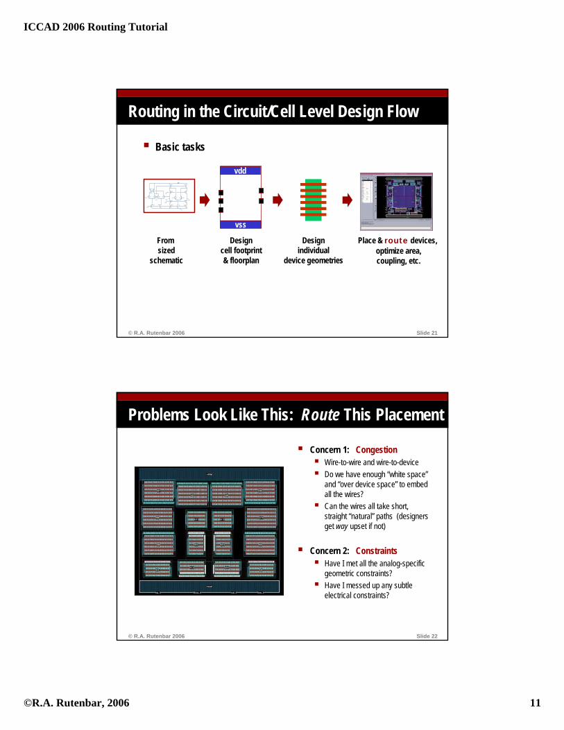
Routing in the Circuit/Cell Level Design Flow
Basic tasks
Vin+ Vin-M2
Vss
Vdd
M9
M11
M7
M5
M8
M10
M4
Vout+Vout�
M17 M16 M15 M14
M6
M19
M1
Vcm
Vout+
M3
Vb2
M12M13
Vb1
M18
Vb3
From sized
schematic
Designcell footprint& floorplan
Designindividual
device geometries
Place & route devices, optimize area,coupling, etc.
vdd
vss
© R.A. Rutenbar 2006 Slide 22
Problems Look Like This: Route This Placement
Concern 1: CongestionWire-to-wire and wire-to-deviceDo we have enough “white space”and “over device space” to embed all the wires?Can the wires all take short, straight “natural” paths (designers get way upset if not)
Concern 2: ConstraintsHave I met all the analog-specific geometric constraints?Have I messed up any subtle electrical constraints?
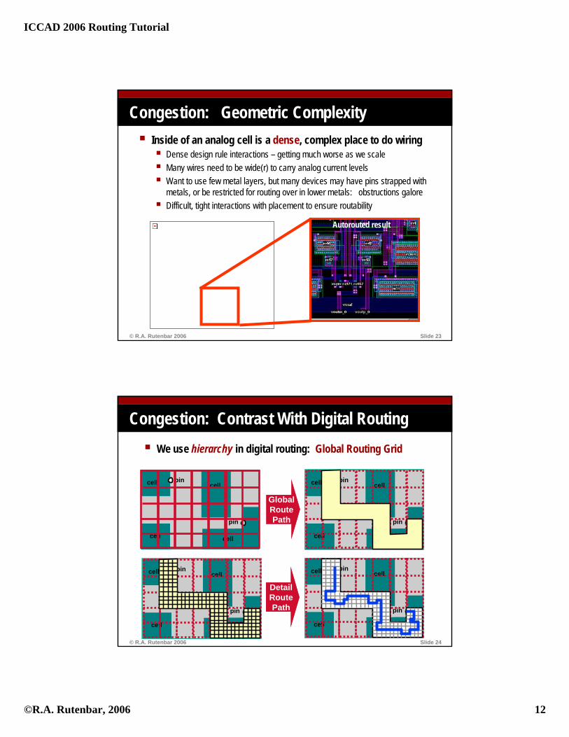
ICCAD 2006 Routing Tutorial
©R.A. Rutenbar, 2006 12
© R.A. Rutenbar 2006 Slide 23
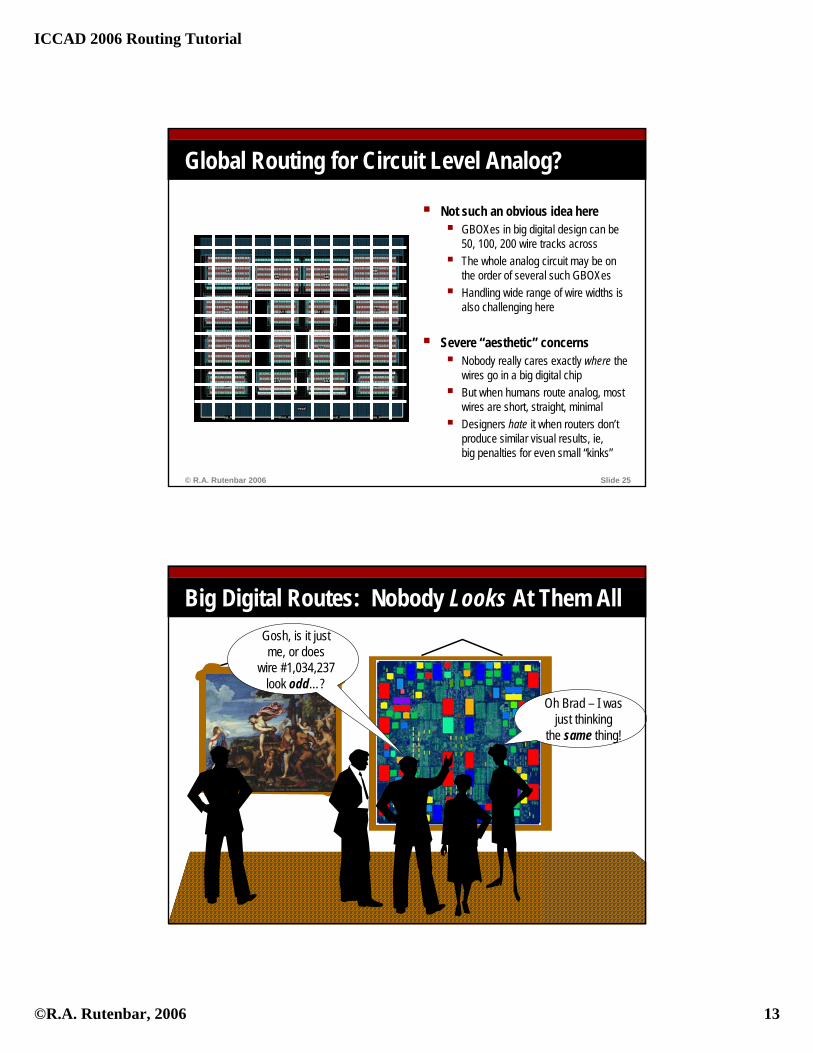
Congestion: Geometric ComplexityInside of an analog cell is a dense, complex place to do wiring
Dense design rule interactions – getting much worse as we scaleMany wires need to be wide(r) to carry analog current levelsWant to use few metal layers, but many devices may have pins strapped with metals, or be restricted for routing over in lower metals: obstructions galoreDifficult, tight interactions with placement to ensure routability
Autorouted result
© R.A. Rutenbar 2006 Slide 24
Congestion: Contrast With Digital RoutingWe use hierarchy in digital routing: Global Routing Grid
pin
pin
cell
cell
cell
cell
pin
pin
cell
cell
cell
cell
GlobalRoutePath
pin
pin
cell
cell
cell
cell
pin
pin
cell
cell
cell
cell
DetailRoutePath
ICCAD 2006 Routing Tutorial
©R.A. Rutenbar, 2006 13
© R.A. Rutenbar 2006 Slide 25
Global Routing for Circuit Level Analog?
Not such an obvious idea hereGBOXes in big digital design can be 50, 100, 200 wire tracks acrossThe whole analog circuit may be on the order of several such GBOXesHandling wide range of wire widths is also challenging here
Severe “aesthetic” concernsNobody really cares exactly where the wires go in a big digital chipBut when humans route analog, most wires are short, straight, minimalDesigners hate it when routers don’t produce similar visual results, ie, big penalties for even small “kinks”
© R.A. Rutenbar 2006 Slide 26
Big Digital Routes: Nobody Looks At Them All
Copyright © 1993, The National Gallery, LondonCopyright © 1993, The National Gallery, London
Gosh, is it just me, or does
wire #1,034,237 look odd…?
Oh Brad – I was just thinking
the same thing!
ICCAD 2006 Routing Tutorial
©R.A. Rutenbar, 2006 14
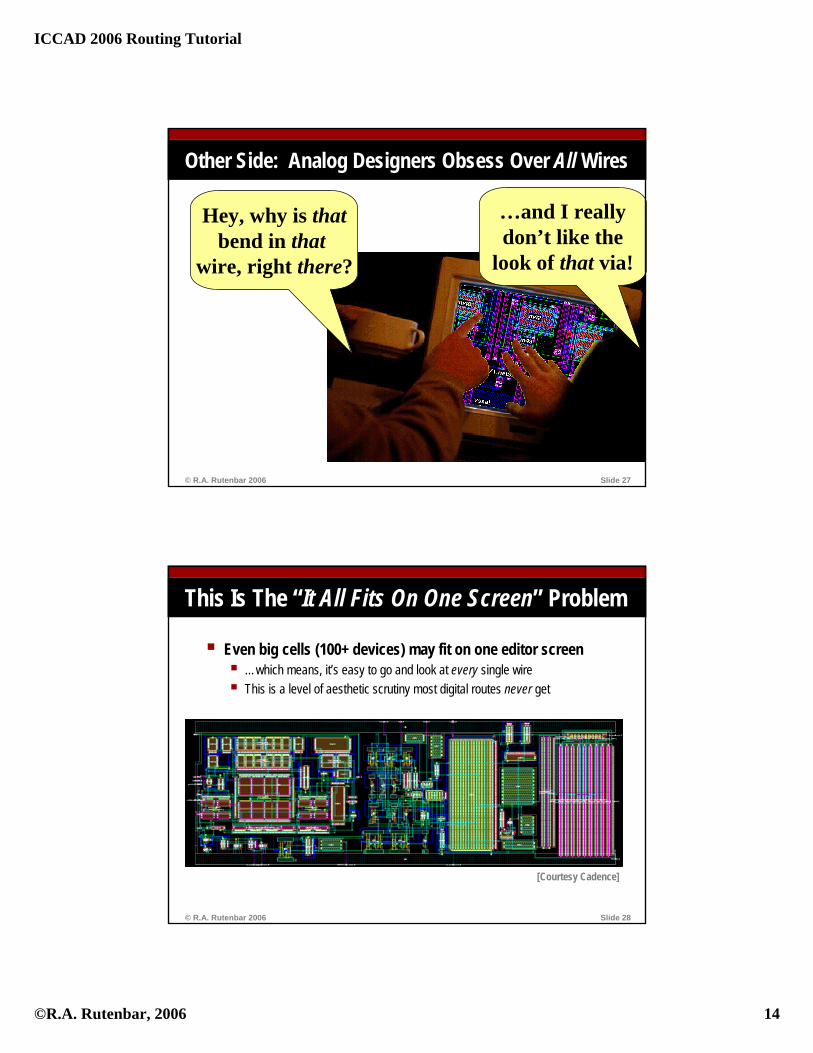
© R.A. Rutenbar 2006 Slide 27
Other Side: Analog Designers Obsess Over All Wires
Hey, why is thatbend in that
wire, right there?
…and I reallydon’t like the
look of that via!
© R.A. Rutenbar 2006 Slide 28
This Is The “It All Fits On One Screen” Problem
Even big cells (100+ devices) may fit on one editor screen…which means, it’s easy to go and look at every single wireThis is a level of aesthetic scrutiny most digital routes never get
[Courtesy Cadence]

ICCAD 2006 Routing Tutorial
©R.A. Rutenbar, 2006 15
© R.A. Rutenbar 2006 Slide 29
Another, Rather Dense “Fits On A Screen” Example
[Courtesy Cadence]
© R.A. Rutenbar 2006 Slide 30
Circuit-Level Routing Issues
Need negotiation-based, ripup-reroute, iterative routing Cannot just route each wire once and assume they all go down “nice”Severe density, congestion issues even in small cells
Need to accommodate a wide range of wire widths (+ via cuts)It just never happens that they all go down at min widthEither need a fully shape-based engine, or a very fancy gridded router
But, also wide range of analog-specific geometric features…

ICCAD 2006 Routing Tutorial
©R.A. Rutenbar, 2006 16
© R.A. Rutenbar 2006 Slide 31
Analog-Specific Geometric Features
Unique attribute of analog is need to balance wiringSupport mirror-symmetric routing, cross-symmetric routing, varieties of incomplete/partially symmetric routing… etc…Guarantee that all routing is exactly geometrically mirrored
Global symmetry line
© R.A. Rutenbar 2006 Slide 32
A Few of the Options for Symmetric Nets
ComplicationsThere are lots of forms of symmetries, letting designers specify them easily is toughSometimes, the pins are “not quite symmetric” or there are a few extra non-symmetric pins on the net. Still need to route “most” of the net as symmetrically as possible
Mirror symmetry Cross symmetry

ICCAD 2006 Routing Tutorial
©R.A. Rutenbar, 2006 17
© R.A. Rutenbar 2006 Slide 33
Symmetric Routing: Basic Trick
Only route one wire, but reflect obstacles from other side across symmetry line, into one shared left-right model of space
Symmetry line
Shared LRmodel, route1 wire here
Reflect single routed wireback across sym line
© R.A. Rutenbar 2006 Slide 34
Balanced Routing
Symmetry is the geometrically easy form of “balance”Sometimes, you don’t have the option, if pins not symmetricIn these case, routing solutions usually look like channels, with extra wiring, and very carefully controlled vias+stubs to balance (capacitance) on nets
12
356
4
21
465
3
Want nets 1-2 to havesame length oneach layer, same # vias
Ditto for nets 3-4, 5-6
ICCAD 2006 Routing Tutorial
©R.A. Rutenbar, 2006 18
© R.A. Rutenbar 2006 Slide 35
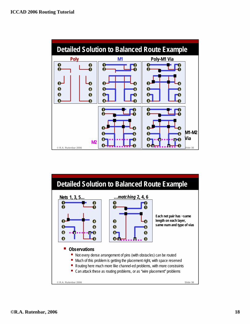
Detailed Solution to Balanced Route Example
12
356
4
21
465
3
12
356
4
21
465
3
12
356
4
21
465
3
12
356
4
21
465
3
12
356
4
21
465
3
x xx x
Poly M1 Poly-M1 Via
M2
M1-M2Via
© R.A. Rutenbar 2006 Slide 36
Detailed Solution to Balanced Route Example
12
356
4
21
465
3
x x
12
356
4
21
465
3x x
Nets 1, 3, 5… …matching 2, 4, 6
ObservationsNot every dense arrangement of pins (with obstacles) can be routedMuch of this problem is getting the placement right, with space reservedRouting here much more like channel-ed problems, with more constraintsCan attack these as routing problems, or as “wire placement” problems
Each net pair has ~samelength on each layer, same num and type of vias
ICCAD 2006 Routing Tutorial
©R.A. Rutenbar, 2006 19
© R.A. Rutenbar 2006 Slide 37
About This Talk
Routing at system-levelAnalog
Frontend
DEVICE
CELL
SYSTEMSYSTEM
© R.A. Rutenbar 2006 Slide 38
What Does System-Level Routing Look Like?Mostly, like a big version of the circuit-level problem
Routing 10s – 100s of basic cells together1K – 10K nets, roughly, connecting ~25K analog transistors + digital stuffVery few min-width nets, lots of balance constraints + avoidance issues
Also, surprisingly, like the device-level problemLots of repeated structures (eg, bits of converter), often want a highly stylized, patterned kind of routing, just like for device-level tasks
[ISSCC’99]J. Vandenbussche, G. Van der
Plas, A. Van den Bosch, W. Daems, G. Gielen,
M. Steyaert, W. Sansen
CURRENT SOURCE ARRAY
SWATCH ARRAY
FULL DECODER
DIGITALCLOCKDRIVER
ANALOGCLOCKDRIVER
Ex: 14-bit 150-Ms/s 0.5um CMOS DAC
Courtesy Georges Gielen, K.U. Leuven

ICCAD 2006 Routing Tutorial
©R.A. Rutenbar, 2006 20
© R.A. Rutenbar 2006 Slide 39
Std cell place/route
DSP Core
PLL ClockResults Converter
( FFT )
Std Cell Place/Route
RAM ( 128 x 16 ) Glue Logic
RAM ( 256 x 16 )
I/O pads
ROM ( 512 x 16A )
ROM CompilerRAM Compiler
[Courtesy Artisan, Cadence]
Small System Ex: Dual-Tone Multi-Frequency DecoderAnalog
© R.A. Rutenbar 2006 Slide 40
Counter (3-bit)
Voltage-ControlledOscillator
Charge Pump
Divider ( 2-bit )
Phase Detector
Buffers
Bias Xtors
Cadence® Generic PDK0.18um 6LM Generic Process
Decoder PLLPushing Inside the PLLLooks like a macroblock digital design – without all glue logic
[Courtesy Cadence]

ICCAD 2006 Routing Tutorial
©R.A. Rutenbar, 2006 21
© R.A. Rutenbar 2006 Slide 41
Bigger Example: Industrial ADC
[Gadient et al, IEEE Electronic Design Proc Workshop, EDP2002]
DACCMP/BIAS
Digital
Level Shifter
© R.A. Rutenbar 2006 Slide 42
What’s Different? Coupling Avoidance IssuesDigital: A small set of relatively simple, discrete fix-it options
Analog: Not so easy.Much closer attention to each critical wire’s parasitics, crossings, neighbors, etc.Still use spacing / shields a lot, but more detailed analysis of parasitic impacts
Xtalk! Dead track Gnd Shield Buffer
fix

ICCAD 2006 Routing Tutorial
©R.A. Rutenbar, 2006 22
© R.A. Rutenbar 2006 Slide 43
What’s Different: Power Distribution
Digital: Grid is not really routedCore rings, around whole chip, around individual macroblocksStripes to bring power to insideDo DC drop analysis, if you don’t like, add more power stripes
Analog: Grid is really routedMaybe not all of it, but lots of itNo nice row/col pattern structureAlso, need to deal with sizing for ohmic drop and electromigration
VSS
VDD
VSS
VDD
VDD
VSSVDD
VSS
VDD
VDD
© R.A. Rutenbar 2006 Slide 44
Summary
Digital routingCapacity: 1-10M nets/pins
Scalability: huge data, CPU time
Route mainly system level
Negotiation-based rip/reroute
Rising DFM complexity hurts
More gridded than shape based
Mostly min width nets
Simple coupling fix-its
Analog routingCapacity: ~100–10K nets, ~25K devices
Scalability: it’s electrical complexity
Route devices, circuits, & systems
Negotiation-based rip/reroute
Rising DFM complexity hurts
More shape-based than gridded
Mostly not min width nets
Not simple coupling fix-its
Analog-specific symmetry/balance/etc
Power grid routing / sizing
ICCAD 2006 Routing Tutorial
©R.A. Rutenbar, 2006 23
© R.A. Rutenbar 2006 Slide 45
To Learn More: Mixed-Signal CAD
Computer-Aided Design of Analog Integrated Circuits and Systems
Rob A. Rutenbar, Georges G. E. Gielen, Brian A. Antao, EditorsHardcover: 768 pages Publisher: IEEEPublished: April 2002ISBN: 047122782X
Book is a collection of essential papers on all aspects of analog and mixed signal synthesis, modeling, layout, etc. Many of the results shown here appear in these papers.


