

Aeroacoustic Measurements in Wind Tunnels
Con DoolanDirector, Flow Noise Group
School of Mechanical and Manufacturing EngineeringUNSW Australia
Sydney, NSW [email protected]
http://www.flownoise.unsw.edu.au

Established in Sydney 1949
55,000 students, 6000 staff
Ranked 48th in world overall (QS)
Ranked 37th in world for Mechanical and Aerospace Engineering (QS)
Largest Engineering faculty in Australia
Produce 25% of Australia’s engineers

Mechanical and
Manufacturing Engineering
Aerospace
Mechanical
Mechanical and
ManufacturingMechatronic
Naval Architecture
Five Teaching Streams in One School
1
2
34
5

UNSW MME Research programs
Mechanical and
Manufacturing Engineering
Advanced Manufacturing
Advanced Structures &
Materials
Tribology and Machine Condition Monitoring
Vibration & Acoustics
Combustion and Solar Thermal Energy
Biofluidics & Micro/Nano Transport
Aerodynamics & Aerospace
Robotics and Autonomous
Systems

UNSW/FNGFlow Noise Group @ UNSW Australia

Our Lab
Fan/ wind turbine noise rig with array
Mach 3 supersonic wind tunnel
UNSW acoustic tunnel: 460 mm x 460 mm
Large wind tunnel: 900 mm x 1200 mm

contribution appears considerably w eakened by the addition of TE serrations. H ow ever, the addition of trailing-edge
serrations also appears to considerably change the noise radiation on the suction side ofthe airfoilatthe low estfrequency,
adding an upstream pointing lobe notpresentin the straighttrailing-edge case.This w as unexpected,especially in lightof
Fig.8. Iso-contours of Q =100 coloured by stream w ise vorticity over the range o x ¼ 7 100,w ith background show ing dilatation rate over the ranger ui¼ 7 7:5 10 2,forcase w ith straight(a)and serrated (b)trailing edge.(Forinterpretation ofthe references to colorin this figure legend,the readeris
referred to the w eb version ofthis article.)
0
f
1e-11
1e-10
1e-09
1e-08
1e-07
1e-06
1e-05
0.0001
pp*
10 20 30 40
Fig.9. Iso-surfaces ofQ =500,coloured by stream w ise vorticity for levels [ 100:100]for D N S ofserrated TE (a).Pow er pressure spectra taken above and
below the airfoilat(x,y)=(0.5,7 0.5)forairfoils w ith straight(---)and serrated (—)trailing edges (b);verticallines denote targetfrequencies and shaded
areas show the range offrequencies used for one-third octave averages aboutthe targetfrequencies.(For interpretation ofthe references to color in this
figure legend,the reader is referred to the w eb version ofthis article.)
Please cite this article as: R.D .Sandberg,& L.E.Jones,D irect num ericalsim ulations oflow Reynolds num ber flow over
airfoils w ith trailing-edge serrations,JournalofSound and Vibration (2011),doi:10.1016/j.jsv.2011.02.005
R.D .Sandberg,L.E.Jones /JournalofSound and Vibration ] (]]]]) ]]]–]]]10
Approximate flow
direction
Serrated
edge
Poroelastic
trailing edge
468 J.W .Jaworskiand N.Peake
FIG U R E 2. Scaling exponentsofK + (kcos✓0)foran elastic edge:(a)exponentof⌦;(b)exponentof✏.
to proceed to an order-of-m agnitude estim ate for the sound am plification factor, β.N oting the sim plifications of ↵1 and ↵2 w hen ⌦2⌧1,a heuristic m agnitude estim ateof(4.16)leads w ith (4.23)to
βe⇠1
⌦K + (kcos✓0). (5.20)
For sm all⌦ in the sense that⌦✏−1/2⌧1, direct substitution of (5.18) yields thescaling estim ate
βe⇠⌦−1/2✏−1/2. (5.21)
Figure 3 confirm s the elastic scattering am plification βe⇠✏−1/2 in this sm all-⌦ lim it,and that in the upper lim it the intrinsic fluid loading param eter has no effect. Thenum erical solutions indicate a transition from βe ⇠ ✏−1/2 to βe ⇠ ✏0 that depends onboth⌦✏−1 and⌦✏−1/2.A m ore com plicated picture em erges in figure 4 for the dependence of thescattered field on the frequency param eter⌦,w here the am plification factor collapsesacross three distinct param eter scalings. O f particular interest is the existence of aregion β ⇠⌦−1/2, predicted by the result (5.21), for the approxim ate finite range0.1✏< ⌦< 0.1✏1/2 as determ ined from figure 4(a,b). Figure 3 indicates that w ithinthis range the am plification dependence on ✏ varies, but the fixed scaling for ⌦furnishes a U 7 velocity dependence forthe far-field acoustic pow er,
⇧ e⇠ u30M4 for✏< 10⌦< ✏1/2. (5.22)
Clearly, the heuristic argum ents to arrive at (5.22) do not hold for ⌦✏−1⌧ 1as show n in figure 4(a). A m ore rigorous approach to determ ine additional scalinginform ation analytically w ould seek to construct a uniform ly valid com positeexpression for βe = βe(⌦,✏) using the Van D yke (1975) m atching principle acrossregions described by ⌦,⌦✏−1/2 and ⌦✏−1. H ow ever, the need to evaluate the edgeconditions for h(↵) in (3.7) com plicates this course of action, and it w ill not bepursued furtherhere.
Direct Numerical Simulation
Theory
+
+
1. Owls fly silently because of
their serrated, poroelastic wings
3. Using new knowledge, develop
and demonstrate a quiet wind turbine
trailing edge.
RMS acoustic
source distributionRotating blades
change ofthe source locations is sm allcom pared w ith the beam w idth (as in CB),there w illbe a large influence from one
source on another source,increasing the overallintegrated 1/12th octave band level.
Fig.11 show s the results ofCB (11a and c)and CLEAN -SC (11b and d)on the top and side sub-arrays individually.CLEAN -
SC of the top array output yields results sim ilar to that of Fig.10b show ing a distribution of 2 lobes on the cylinder axis
caused by axialvariation of vortex shedding frequency.Conversely,CLEAN -SC of the side array only captures one source
closestto the array.This is unsurprising as the side array cannot‘see’the sources behind one another w hen the w avelength
is large.W hen Fig.11b and d is m ultiplied together,the disparity in the y-position ofeach ofthe lobes causes the elongated
lobe seen in Fig.10d.Evidently,because the lobes do not appear in exactly the sam e spatialpositions in the top and side
array CLEAN -SC outputs respectively, there is significant cancellation w hen m ultiplied together. This causes a large
reduction in source am plitude as seen in Fig.10d.D espite this severe under-prediction of source am plitude,the source
localisation is stillvery satisfactory.
Fig.12 show s the beam form ing results ofthe finite airfoilat a centre band frequency of4 kH z.Atthis frequency,w ide-
band trailing edge noise dom inates the noise spectrum [4].It is im m ediately clear that in this case,CB (Fig.12a) does not
yield a source m ap that can be interrogated easily.G eneralinspection ofthe m ap indicates that noise is generated by the
portion of the trailing edge that is closest to the airfoil–w all junction and also the airfoil–w all junction itself.H ow ever,
because of the highly elongated m ain lobe in the z-direction,it is unclear w hether the noise is located along the plate
surface or at the trailing edge ofthe airfoil.
M B (Fig.12c)yields m ore interpretable results.Because the m ain lobe is separated from the side-lobes,the m ap clearly
show s noise generated across the w hole trailing edge.Itis also apparentthatnoise is generated from the leading edge atthe
airfoil–w alljunction as w ellat the entire airfoil–w allinterface.
Fig.12. Experim entalbeam form ing source m aps ofa finite airfoilatthe 4 kH z 1/12th octave centre band frequency using CB (a),CCS (b),M B (c)and M CS
(d).The colourbar denotes the bias (uncorrected)source strength (dB re.20 μPa).(For interpretation ofthe references to colour in this figure caption,the
reader is referred to the w eb version ofthis paper.)
R.Porteous et al./JournalofSound and Vibration 355 (2015) 117–134132
Experimental Aeroacoustic Beamforming
2. Joint numerical, theoretical and
experimental methodology to understand
underlying mechanics
Air flow3D acoustic
source
Airfoil model
Wind tunnel outlet
dB
Major projects: TE noise

NASA Image 2014
Green Aviation: Lower Emissions of Carbon AND Noise#1 Civil aviation technical problemBUT - Lean Burn = more noise!
8

Aircraft relative noise levels
Leylekian, L., M. Lebrun, and P. Lempereur. "An overview of aircraft noise reduction technologies." AerospaceLab 6 (2014): p-1.

Goines and Hagler • Noise Pollution: A Modern Plague, Southern Medical Journal • Volume 100, Number 3, March 2007
Environmental Noise Pollution
• Form of air pollution and a threat to health and well-being
• Widespread problem that will continue to worsen because of– Population growth– Urbanisation– Sustained growth in highway, rail, and air traffic
• Impairs health and degrades residential, social, working, and learning environments
• High Economic and Social costs, now and in the future.


Selected Effects of Environmental Noise Pollution
Hammer MS, Swinburn TK, Neitzel RL. 2014. Environmental noise pollution in the United States: developing an effective public health response. Environ Health
Perspect 122:115–119; http://dx.doi.org/10.1289/ehp.1307272

Aeroacoustic Wind Tunnel Measurements
• Controlled conditions: essential to understand noise generating physics
• High quality data: needed for models and validation of computational models
• Can test design changes, develop laws, models etc
• Needs special facilities and instrumentation

Anechoic Wind Tunnel
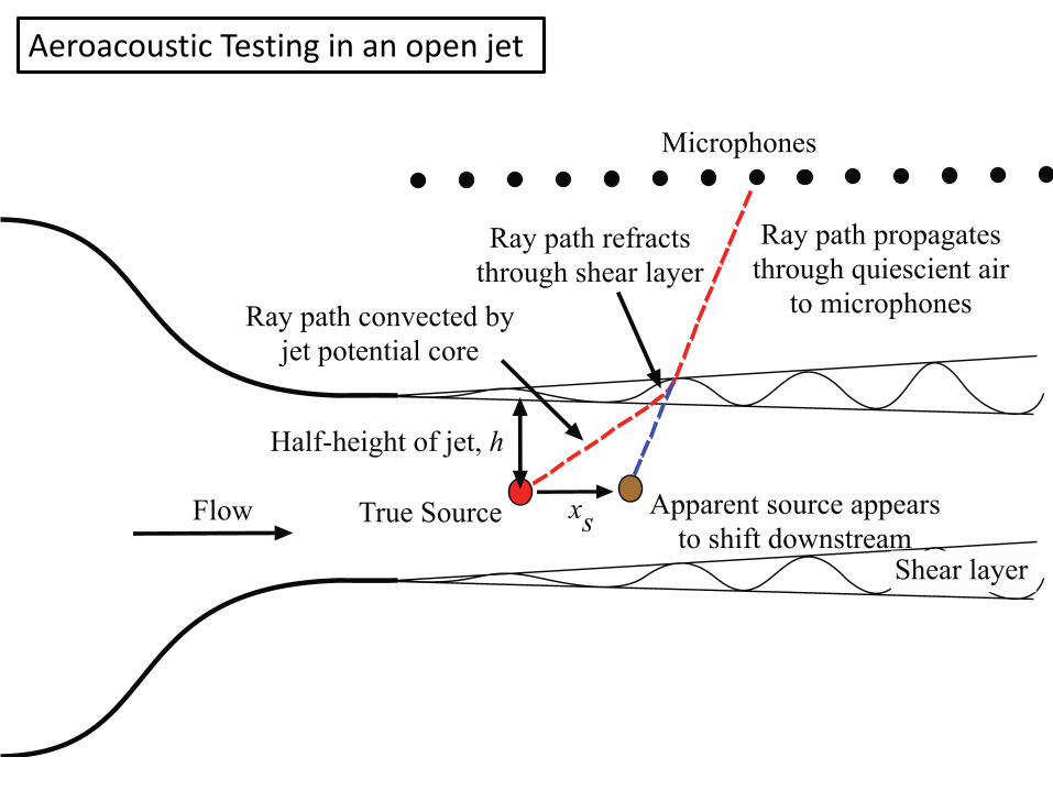
Aeroacoustic Testing in an open jet

Conventional hard-walled closed return wind tunnel
Testing environment noisy andReverberant: Makes acousticMeasurements difficult, but notimpossible!

We wish to localise acoustic sources on the scanning grid
Beamforming Principles

Delay and Sum
When time (phase) is identical at each microphone, array signal is a maximum: source “localised”
m = Nm = 1
m

Frequency Domain Beamforming: Mathematics I
Cross-spectralmatrix (CSM)
Each element of CSM
Complex Conjugate of
= pressure signal on microphone m

Frequency Domain Beamforming: Mathematics II
Steering vectors
Phase between microphone m
and scanning point
Beamformer output: Power Spectrum Vector
Vector of steering locations for each microphone

Beamformer Frequency limits: Rayleigh criterion and spatial aliasing
= Desired resolution (source separation distance)
z = Distance between array and source D = Array size or aperture
High-frequency limit:
Set by spatial aliasing
Low-frequency limit:
Set by Rayleigh criterion
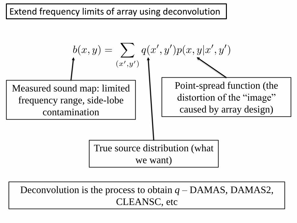
Extend frequency limits of array using deconvolution
Measured sound map: limited
frequency range, side-lobe
contamination
True source distribution (what
we want)
Point-spread function (the
distortion of the “image”
caused by array design)
Deconvolution is the process to obtain q – DAMAS, DAMAS2,
CLEANSC, etc
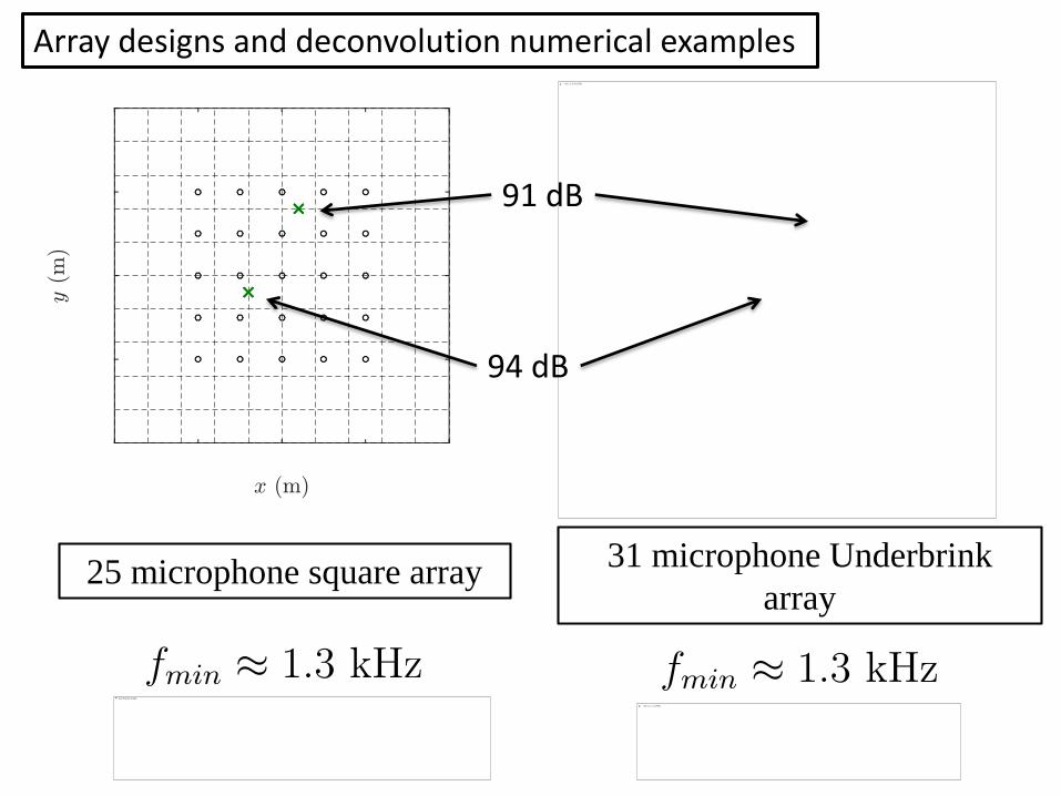
Array designs and deconvolution numerical examples
25 microphone square array31 microphone Underbrink
array
94 dB
91 dB

Square array: conventional beamforming
Reasonable low frequency resolution, very poor high frequency resolution

Underbrink array: conventional beamforming
Better resolution at higher frequencies, fewer side lobes

CleanSC: improves beamformer output

Small Anechoic Wind Tunnel

62-channel orthogonal beamforming array in small anechoic wind tunnel

Experimental test case: cylinder in cross-flow
2 kHz 6 kHz

Shear-layer correction
Padios/Valeau
Amiet/Koop
Ray Tracing
2 kHz 6 kHz

3D Beamforming
Scanning volume
Multiplicative beamforming principle

Experimental 3D Beamforming: Cylinder
Conventional
Multiplicative Multiplicative + CLEANSC
Conventional + CLEANSC

Experimental 3D Beamforming: Wall mounted airfoil
Conventional Conventional + CLEANSC
Multiplicative Multiplicative + CLEANSC

UNSW 64 Channel Optimised Array

Chosen Array Design
• 7 circles, 9 microphones per circle + 1 in centre

Rotor Rig – in Anechoic Chamber
Rotor Rig – in Wind Tunnel

Conventional Beamformingf=1.2kHz f=2.3kHz
f=3.5kHz f=7.0kHz
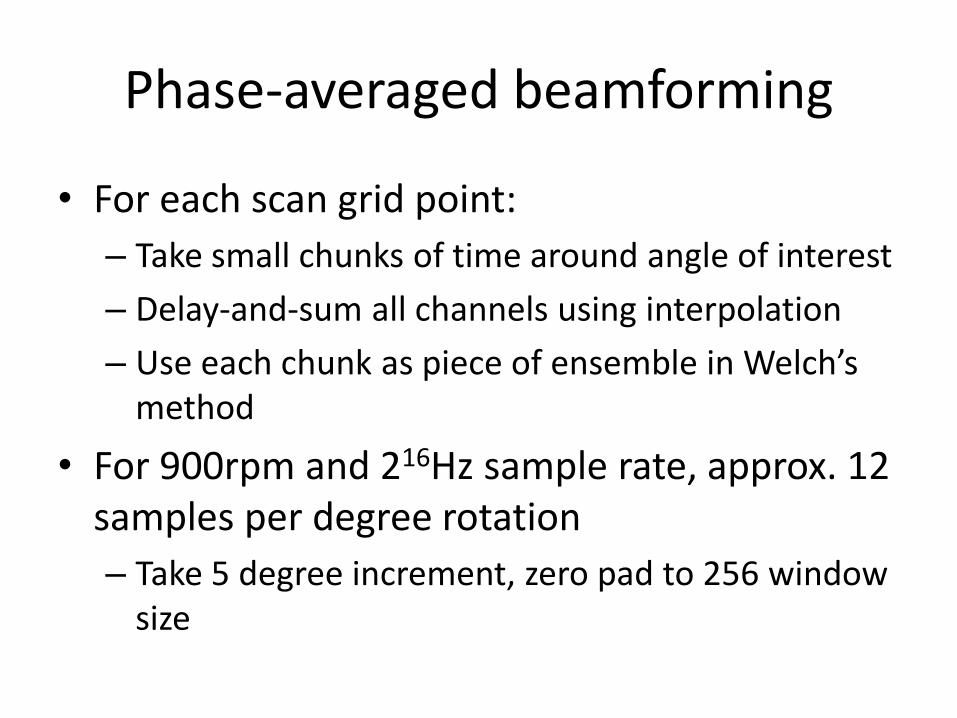
Phase-averaged beamforming
• For each scan grid point:
– Take small chunks of time around angle of interest
– Delay-and-sum all channels using interpolation
– Use each chunk as piece of ensemble in Welch’s method
• For 900rpm and 216Hz sample rate, approx. 12 samples per degree rotation
– Take 5 degree increment, zero pad to 256 window size

Phase-averaged Beamforming
• θ=0°
f=2.5kHz f=4.6kHz
f=7.2kHz f=12.8kHz

Newer phase-averaged results
f=2.0kHz

Newer phase-averaged results
f=4.1kHz

Newer phase-averaged results
f=11.0kHz
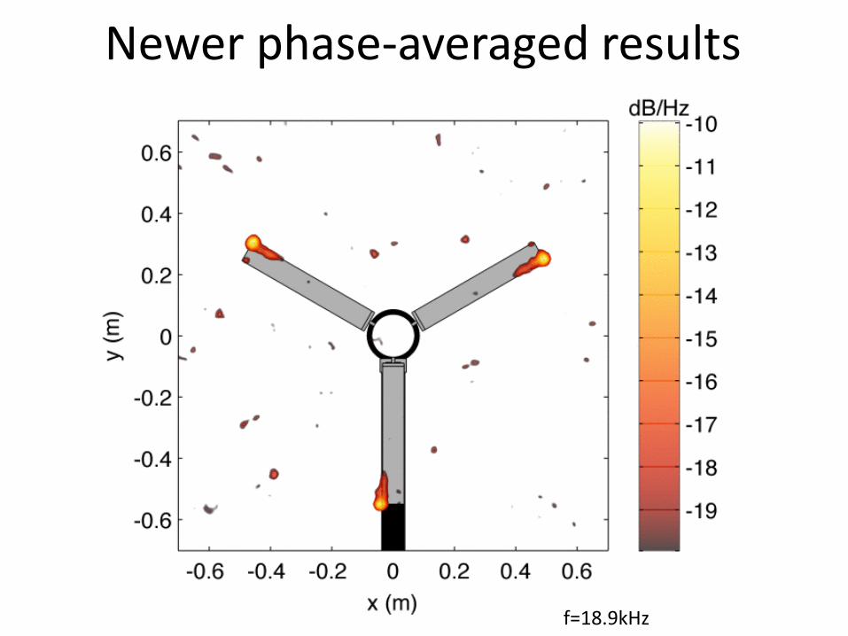
Newer phase-averaged results
f=18.9kHz

Beamforming in hard-walled wind tunnels

Test Case: Speaker as source in closed-section wind tunnel

Numerical Green’s function: image source model
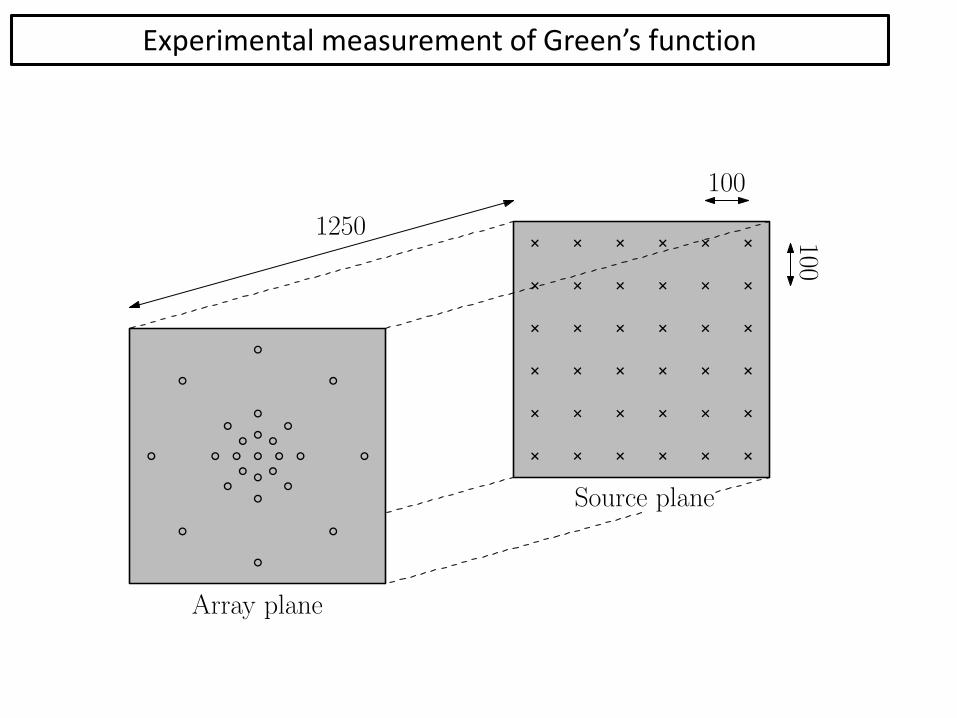
Experimental measurement of Green’s function

Results – use of conventional, numerical and empirical Green’s functions
Conventional Numerical
Empirical

Axial Fan Noise: Experiments and semi-empirical modelling
Aim is provide new understanding of broadband and tonal noise production + data for validation of models

Measurement of broadband and tonal noise from axial fans
Dimensions in mm
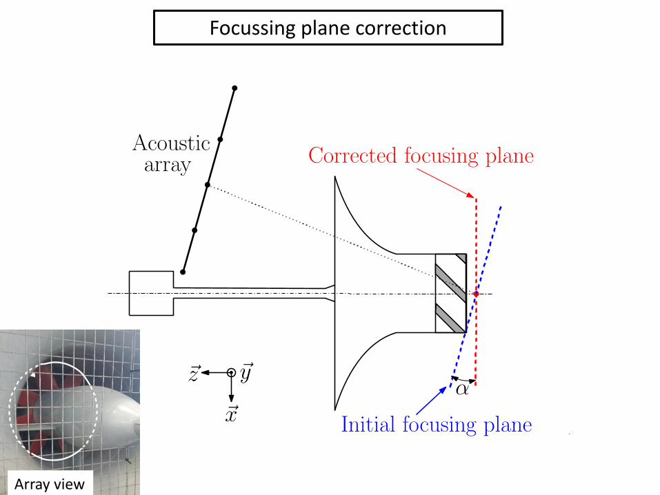
Focussing plane correction
Array view

Composite Beamforming
Left Array Right Array Left+Right Array

Composite Beamforming: 10 kHz
Left Array Right Array Left+Right Array

Experimental Green’s function measurement
Speaker used at 8 locations as broadband
source, response measured on array

Experimental Green’s function measurement: left array only
Our next step is to determine complete Green’s function using composite method and correct
beamformer output

Semi-empirical modelling of axial fan noise
Frequency (Hz)10
210
310
4
PS
D (
dB
/Hz)
0
20
40
60
80
100
120
Frequency (Hz)10
210
310
4
PS
DW
(d
B)
20
40
60
80
100
120
Blue = ExperimentBlack dashed = Amiet
Blue = ExperimentBlack dashed = CarolusIn each case, an experimental transfer
function was used to account for propagation from the rotor plane top to the microphone.
!"#$%&''()*+,%
-.$/&.#(%-01$%
23$3/%
456%78-9%
-% :% ;%
<%!%=%
=&.%
>?((@%A3B%C%
DEFD%)%
DEFD%)%
DEGG%)%
DEH%)%
DEH%)%
DEI%)%
DEI%)%

Mine Ventilation Fans: 100-120 dB(A) @ 1.5 mRequire noise reduction without performance loss
BHP Appin Coal mine, 18 cu.m mine ventilation fan #138

Microphones A and BBlade pass tonesMachinery noise

Comparison with models: Microphone A

Time Reversal - Principle


Time Reversal – Experimental dipole visualisation using CAA code
Includes effects of contraction walls and PTRSL super-resolution

Time Reversed RMS pressure
784 Hz
1208 Hz
1584 Hz

TR – Trailing edge noise example

1250 Hz 1600 Hz 2000 Hz
2500 Hz 3150 Hz 4000 Hz

Thank-you!
• All this work has been performed by my students, postdocs and colleagues in my group – thank you team!
• The work has been mainly funded by the ARC and DSTO – many thanks to them too.
• Any Questions?


