

U NIVERSITY OF ILLINOIS
URBANA
AERONOMY REPORTNO. 64
(NASA-CR-142344) STUDIES OF THE N 75-19889DIFFERENTIAL ABSORPTION ROCKET EXPERIMENT(Illinois Univ.) 96 p HC $4.75 CSCL 04A
UnclasG3/46 13466
STUDIES OF THE DIFFERENTIALABSORPTION ROCKET EXPERIMENT
by
J. C. GintherL. G. Smith
January 15, 1975
Library of Congress ISSN 0568-0581
Aeronomy Laboratory
Supported by Department of Electrical Engineering
National Aeronautics and Space Administration University of Illinois
NGR 14-005-181 Urbana, Illinois
https://ntrs.nasa.gov/search.jsp?R=19750011817 2018-05-29T03:52:26+00:00Z

CITATION POLICY
The material contained in this report is preliminary information cir-culated rapidly in the interest of prompt interchange of scientificinformation and may be later revised on publication in acceptedaeronomic journals. It would therefore be appreciated if personswishing to cite work contained herein would first contact the authorsto ascertain if the relevant material is part of a paper published orin process.
UILU-ENG 75 2501
AERONOMY REPORT
N 0. 64
STUDIES OF THE DIFFERENTIAL ABSORPTION ROCKET EXPERIMENT
By
J. C. GintherL. G. Smith
January 15, 1975
Supported By Aeronomy Laboratory
National Aeronautics Department of Electrical Engineeringand Space Administration University of Illinois
Grant NGR 14-005-181 Urbana, Illinois

ABSTRACT
Investigations of the ionosphere, in the rocket program of the
Aeronomy Laboratory, include a propagation experiment, the data from
which may be analyzed in several modes. This report considers in
detail the differential absorption experiment. The sources of
error and limitations of sensitivity are discussed. Methods of
enhancing the performance of the experiment are described. Some
changes have been made in the system and the improvement demonstrated.
Suggestions are made for further development of the experiment.

TABLE OF CONTENTS
Page
ABSTRACT . . . . .................. . . ii
TABLE OF CONTENTS ................. . ...... iii
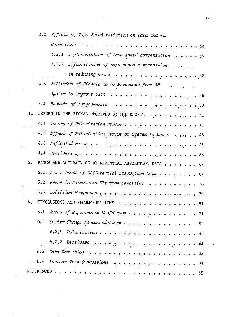
LIST OF TABLES . . . . . . . . . . . ... .. . . . . . . . . . v
LIST OF FIGURES . . . . . . . . . . . . . . . . . . . . . ... . vi
1. INTRODUCTION . . . . . . . . . . . . . . . . . .. . ...... * * 1
2. THEORY AND IMPLEMENTATION OF THE PROPAGATION EXPERIMENT . . . . 3
2.1 The Theory of Appleton-Hartree Under Quasi-
Longitudinal Propagating Conditions .. . . . . .. . 3
2.2 The Sen-Wyller Theory . . . . . . . ... . . . . 8
2.3 Operations of the Experiment . . . .. . . . . . . . 10
2.4 Procedures for Recovering Rates of Differential
Absorption . . . . . . . . .. . * .* * * * * * 19
2.4.1 Computer determination of electron concentration
from differential absorption rates .........* * * * * * 21
3, IMPROVEMENTS MADE IN DATA ACQUISITION AND REDUCTION SYSTEMS .* 23
3.1 FM Data System . . ........ . ... . . . .... 23
3.1.1 Theoretical superiority of frequency over
ampZitude modulation as a data link . ....... 23
3.1.2 Design of frequency modulated data link . * * *.... 26
3.1.3 Data reduction with frequency modulated system * *. 29
3.1.4 Verfication of data link improvement by use of
FM system . . . . . . . . . . . . . . . . . 34
iv
3.2 Effects of Tape Speed Variation on Data and its
Correction . . . . . . . . . . . . . . 34
3.2.1 Implementation of tape speed compensation ... . . 37
3.2.2 Effectiveness of tape speed compensation
in reducing noise . . . .. . . . .38
3.3 Filtering of Signals to be Processed from AM
System to Improve Data . * * * * * * * . .. . 38
3.4 Results *of Improvements . . .. ..... .. .... . . 38
4. ERRORS IN THE SIGNAL RECEIVED BY.THE ROCKET ...... . 41
4.1 Theory of Polarization Errors . . . . . . . . 41
4.2 Effect of Polarization Errors on System Response .. .. 46
4.3 Reflected Waves ......... . . .... o ,i... 53
4.4 Receivers .... ...... * * * * .. ...... . 58
5,. RANGE AND ACCURACY OF DIFFERENTIAL ABSORPTION DATA ... . . . 67
5.1. Lower Limit of Differential Absorption Data . . .. 67
5.2 Error in Calculated Electron Densities ... ........ 76
5.3 CoZZision Frequency *...... , .. . .. .. 79
6. CONCLUSIONS AND RECOMMENDATIONS ..... ... . . .. . . . 81
6.1 Areas of Experiments Usefulness . ........... 81
6.2 System Change Recommendations .. ... 0 ... 0 81
6.2.1 Polarization .. * * * .. ......... . . 81
6.2.2 Receivers * ..... * * * *... .. 0 0 .. 0 . 83
6.3 Data Reduction . . . .. ... . . .. . . . . . 83
6.4 Further Test Suggestions 0...... ... . . . . 0 84
REFERENCES . . . . . . . . . . . . . . . 85

V
LIST OF TABLES
Page
3.1 Test of Data Transfer System .. . . . . . . . . . ... . 35
3.2 Test of Tape Speed Compensation on Data from 14.514 . . .. 39
3.3 Filter Test on 14.361 . . . . . . . . . . . . . . . . .. . 40
4.1 Received Frequencies Including Polarization Errors . . . . . 45
4.2 Power Differences, Useful Data Range, and Limit of
Data in Time and Altitude for Three Rocket Flights ..... 54
4.3 Frequencies in Receiver Output when Reflections are
Present for rr << 1 and R << ... . . . . . ... . 56X' O
4.4 Receiver Output for T = - 1 and R = 0 . . . . . . . . . 59
4.5 Stations Near 3.385 Mz .. . . . . . . . . . . . . . . 64
4.6 Stations Near 5.040 MHz ...... . . . ........ 65
4.7 Extra Signals Detected by Receiver #106 in
5040 Payload . . . . . . . . . . . . . . 66
5.1 14.511 - 2.225 and 3.385 KHz Differential
Absorption Rates . . . ............... . 68
5.2 14.513 - 2.225 and 5.04 MHz Differential
Absorption Rates .......... ......... ... 69
5.3 14.514 - 2.225 and 5.04 MHz Differential
Absorption Rates ................. . . ...* * 71
5.4 Lower Limit of Data ........ .. . . . . ........ . . 72

vi
LIST OF FIGURES
Figure Page
2.1 Appleton-Hartree versus Sen-Wyller differential
absorption index per unit electron concentration
as a function of electron collision frequency.
The approximate Appleton-Hartree curve is nor-
malized to.agree with Sen-Wyller curve for
vanishing collision frequency [Mechtly et al.,
1967] . . . . . .................. . . . . . . . . . 11
2.2 Original system block diagram [Knoebel et al.,
1965] ................. . . . . . . . . . . . . 13
2.3 Generation of polarization ellipse (adapted from
Salah and Bowhill [1966]) . .. .. . . . . . . . . . 14
2.4 Section of chart record for Nike Apache 14.513
showing differential absorption signals in re-
lation to lower band edge (LBE), band center (BC)
and upper band edge (UBE). This illustrates the
AM system . ... . . .. .. . . . ... . .. ..... 17
2.5 Section of chart record for Nike Apache 14.511
showing differential absorption signals in rela-
tion to lower band edge (LBE), band center (BC)
and upper band edge (UBE). This illustrates the
FM system . . . . . . . . . . . .. ... ..... . . 18
2.6 Block diagram of digitizing process. . .. ... . . . 20
3.1 Block diagram of amplitude modulated data link . . . 24

vii
Figure Page
3.2 Block diagram of frequency modulated data
link . . . . .................. . . . . . . . . 27
3.3 Measured frequency response of four data
lines at Wallops Island, shown in relation to
IRIG channels 1 to 10. ................ . 28
3.4 Possible AM system data. . ... ......... . . . 30
3.5 Possible FM system data. ...... . ... . . . . . 31
3.6 Flowchart of original DAPROC program. This
flowchart is a corrected version of that
given by Slekys and Mechtly [1970]. The
program listing in that reference is correct
and is currently stored on the IBM 360 . ....... 32
3.7 Tape speed error . .................. 36
4.1 Profiles of probe current (upper scale) and
electron density (lower scale). Data from the
differential absorption experiment along are
shown. . .... . . .... . .. . .. ..... 47
4.2 Profiles of probe current (upper scale) and elec-
tron density (lower scale). Data from the
differential absorption experiment along are
shown. . . . . . . ........... . ..... 48
4.3 Profiles of probe current (upper scale) and
electron density (lower scale). Data from the
differential absorption experiment alone are
shown. . . . . . . . . . . . . . . . . . . . . . . 49

viii
Figure Page
4.4 Frequency components at receiver output . .. ..... 50
4.5 Frequency components at receiver output. . . . . . . . 51
4.6 Frequency components at receiver output. . ... .. .. 52
4.7 Section of chart record for Nike Apache 14.520
showing differential absorption signals in
relation to lower band edge (LBE), band
center (BC) and upper band edge (UBE). This
is the FM system used for a nighttime flight ... . . 57
4.8 Frequency spectrum of receiver output sig-
nal for Nike Apache 14.270, prepared by
K. L. Miller [Edwards, 1973].
4.9 Noise temperature at medium and high
frequencies [Jordan and Balmain, 1968].
5.1 Profiles of probe current (upper scale) and
electron density (lower scale) . ... ........ . 73
5.2 Profiles of probe current (upper scale) and
electron density (lower scale) . ... ...... . . 74
5.3 Profiles of probe current (upper scale) and
electron density (lower scale) . ........... 75
5.4 Estimated error in electron density 77
5.5 Standard error of 1/10 sec data taken over one
second . . . . . . ...... . . . . . . . . . . . 78
5.6 Electron densities using different collision
frequency models ... ... . . . . . . . . . . . . 80

i. INTRODUCTION
The propagation experiment has been used on all rocket flights con-
ducted by NASA for the University of Illinois' Aeronomy Laboratory. The
experiment was designed by the Coordinated Science Laboratory for use in
the IQSY years of 1964 and 1965. The experiment measures two phenomena,
differential absorption and Faraday rotation. Faraday rotation is the
phenomenon of the changing phase characteristics between two propaga-
ting modes, while differential absorption is characterized by a dif-
ference in attenuation rates. These two phenomena can be used together
to determine electron concentrations and electron collision frequencies,
or independently, by use of suitable approximation, for calculation of
electron densities. The electron densities used to calibrate probe ex-
periments, carried by the rockets, are capable of measuring fine
structure in the electron concentration, but not absolute magnitudes.
This report is concerned with operation of the differential absorp-
tion experiment without use of the accompanying Faraday rotation data.
The objectives are to determine criteria for determining valid data and
improvement of the accuracy of measurements. It is desired to be able
to measure electron concentrations as low as 10 cm- 3 . To accomplish this
the errors in the absorption rates measured on daytime flights must be
reduced to about .01 dB/sec. For nighttime flights the objective is to
reduce the errors from values over 1 dB/sec often seen, to values of
about .1 dB/sec.
Chapter 2 gives a summary of the theory of the propagation ex-
periment as it applies to differential absorption. Chapter 3 describes
improvements made in the operating and data-reduction systems. Chapter 4
covers errors in the experiment resulting from unwanted signals which are
not included in the theory of the experiment's design. Chapter 5 dis-
cusses the range of valid data and how this should be defined in future
work. Finally, Chapter 6 contains suggestions for system improvements
which can be made without major redesign of the experiment.

3
2. THEORY AND IMPLEMENTATION OF THE PROPAGATION EXPERIMENT
To gain an understanding of how the propagation experiment is designed
to operate, the theory developed by Appleton [1932] and Hartree [1931]
provides an excellent working base. This theory has been improved upon by
Sen and Wyller [1960] but the Appleton-Hartree equations provide the
necessary tools to understand the experiment and are the basis upon which
the experiment was designed.
The following sections will present an outline of the Appleton-Hartree
theory and how this is changed by Sen and Wyller. Then a description of
how the experiment is designed and an outline of the data reduction pro-
cess will be presented.
2.1 The Theory of Appleton-Hartree Under Quasi-Longitudinal Propagating
Conditions
In a region of free electrons, such as the earth's ionosphere, where
there is a magnetic field present the medium becomes bi-refringent. This
means that a traveling wave entering this medium will be split into two
elliptically polarized modes, each mode subject to a different index of
refraction. The theory of Appleton-Hartree determines the modes of prop-
agation and the indexes of refraction of these modes in the earth's
ionosphere under the following assumptions: electron collisions with neu-
trals are independent of electron energies, the medium of propagation is
electrically neutral with a uniform charge distribution, the magnetic
field is uniform throughout the medium, and the ions, because their masses
are much greater than that of an electron, are stationary. The theory
follows:

Assume a vertically propagating wave which has the form
E = E exp[j(wt - kz)] (2.1)
k is the propagation constant, w is the operation frequency, and E0 a
reference field
E =E x+E y. (2.2)o x y
The polarization of this wave is defined as
ER = E- (2.3)
If the fields are in the form of equation (2.2) they will have
refraction indices given by
P P2 x _k
n = 1 + 1 + - (2.4)EE EE (2.4)oz o y W/Eoo °
In the above, P and P are the polarization fields in the x and y direc-x y
tions. The motion of the free electrons in the ionosphere will be governed
by the equation of motion:
mr + mvr = - e( x B -eE (2.5)
v is the electron-neutral collision frequency, and B the magnetic flux.
The polarization can be found from the electron displacements as

P = - N er (2.6)
where N is the electron density.
Before continuing the development of the theory, the following table
of standard symbols is presented.
V
X -H
N is the plasma frequency and is defined as
Ne2
-N =0
WH is the gyrofrequency defined as
eB-H m
which is divided into two components, one along the direction of propa-
gation and one transverse to the propagating wave.
With the above set of symbols, equations (2.5) and (2.6) can be com-
bined to form

6
-1E E = M P (2.7)O -
where -
1 - jz jYL - jT
M-1 - -X -jY 1 - jZ 0
j0r 0 1 - jZ
When this result is combined with Maxwell's equations, the characteristic
equation for the polarization becomes
2
R2 + 1-X-jZ R + 1 = 0 (2.8)
which when solved for the polarization yields
2 F 4 2YT /2Y + T /4YL2
R = -j + 1+ (2.9)-Z +-X-JZ (2.9)
and the solution for the refractive index is
2 Xn = 1 - (2.10)1 - jZ - jYLR
which is known as the Appleton-Hartree formula.
For rocket flights from Wallops Island, with which this study has
been primarily concerned, the equations can be simplified since the direc-
tion of propagation is approximately along a magnetic field line so that

7
2
<< 1 - X - jZ2YL
is valid.
When this approximation is used inequations (2.9) and (2.10), the
results are
R = d (2.11)
2 Xn = 1 - -jZ YL (2.12)
The solution for R indicates two circular modes will be propagated. The
+j is known as the extraordinary mode and the -j as the ordinary. In the
refractive index relation, the plus sign on YL is associated with the
ordinary mode and the minus with the extraordinary mode.
A further approximation in the equations may be made on the basis
that the plasma frequency in the D and E regions where the experiment is
intended to be used, is much smaller than the frequency of the propagating
wave used in the experiments, thus
X << 1 (2.13)
Using (2.13) in (2.12) yields
SX2n = 1 1-j3Z + Y (2.14)

The index of refraction is divided into its real and imaginary parts
n = m + j X (2.15)
2X (1 t YL) Xn= I - 2 - 2 2
(1 +_ Y) +Z ( 1 + Y ) + Z
and the equation for the propagating wave may be written as
E = E exp(-Xk Z) exp[j(wt-pk Z] (2.16)
This is the equation of a wave which decays in amplitude as it propagates.
It is this phenomena described by the coefficient of absorption
K = ko X (2.17)
with which this study is concerned.
2.2 The Sen-Wylter Theory
An improvement on the Appleton-Hartree theory was developed by Sen
and Wyller [1960] to correct the assumption that the collision frequency
is independent of electron energy. The collision frequency is assumed to
have the form
v = Vm f(v) (2.18)
f(V) is a function of the electron velocity which is assumed to be
Maxwellian. The theory is quite complicated and will not be reproduced
here.

9
The result of the. theory is to give an index of refraction
n = A + B sin2 ± B2 sin 42 - C cos24. (2.19)
D + E sin 2)
-- is-the-angle between the wave normal-and-B_, -wi-ththe other variables--
defined as follows:
A = 2 i(eii + III)
C= 2 zI II
D= 2
E = 2
I I, and 6 are the dielectric tensor elements defined as
S = (1-a) -j b
S= (f-d)/2 + i(c-e)/2
= [a-(c+e)/2] + j [b - (f+d)/2],
in which a, b, c, d, e, and f are functions of the # script integrals

10
o
1.(X) - 2 e dF (2.20)o (62 + X )
2
5 7 wm 2.5 72
N (W-WH) 0-wHc =2-.5WV m
e = 2 1. 5m m2
5mwN /W +WHd =
2wv y 2.5 v5
2
2.3 peration of the Evperiment
two modes are transmitted from the ground to a rocket 2 .as it passes through
Figure 2.1 shows how the Sen-Wyller and Appleton-Hartree theories
differ, especially at high collision frequencies found at the lower alti-
tudes. It is clear from this that the full Sen-Wyller theory will be
necessary for analysis below 85 km.
2.3 Operation of the Experiment
In order to measure the absorption properties of the atmosphere, the
two modes are transmitted from the ground to a rocket as it passes through

10 - -_____ __ _- -
APPLETON-HARTREE EQ.NIKE APACHE 14.143
vYL /( I-Y 2 )2
X<< I
Z2< <(-YL)2
o
J.G.R. 65, 3931 (1960)
13
105 106 U (l) 107 10a
:90 80 70 60 50
h (km).
Figure 2.1 Appleton-Hartree versus Sen-Wyller differential absorption index perunit electron concentration as a function of electron collision frequency.The approximate Appleton-Hartree curve is normalized to agree with Sen-Wyller curve for vanishing collision frequency [MechtZly et al., 1967].

12
the ionosphere. By measuring the differences in the rate of absorption of
the two modes (differential absorption) and combining the results with the
Faraday rotation experiment, or by using a collision frequency model, the
electron concentration of the ionosphere can be measured.
A block diagram of the original system is shown in Figure 2.2. The
signal generated by the configuration consists of an ordinary wave at fre-
quency fo - 6, where 6 is 250 Hz, and an extraordinary wave at fo + 6.
The resultant wave can be visualized as an electric vector of frequency fo
spinning in the ordinary direction with a frequency fo - 6. The magni-
tude of the vector is governed by an ellipse spinning at frequency 6 in
the ordinary direction as shown in Figure 2.3. The above as'sumes the
ordinary magnitude is larger than the extraordinary and that 6 is
positive.
Analytically, the result can be shown by taking the ordinary wave to
be
A ]i Q sin[(w-6)t - k Z] - j Q cos[(w-6)t - koZ]
The extraordinary wave is then taken as
i R sin[(w+6)t - k Z] + j R cos[(w.i)t - k Z]
k and kx are the propagation constants for the o(ordinary) wave and the
x(extraordinary) wave.
The unit vector for the rocket antenna spinning at w may be written
as
a =- isinw t + j cosw t (2.21)

13
CSL- van Rocket PayloadAudio Osc I I I
SLinear Pot ReceiverPhase En DetShifter
Exciter X0 Attenuator 0
SAtten torAttenutor D
if fe re nt ial -Phase Manual SCO
Detector Attenuator7-7heeeee e]tControl
ose Adder Power I TeleetryShifter " Tronsmitter
ExciterX -- Atten a t or X
A e -
rI
Linear Poto ierServo - IMotort
Toceh Audio Osc
FB
ChopperAmplifier
% ModDiscrim.
Quick Look
OD,., oAttenuator X Position
Rocket Rcvr. Output
500 CPS Phase Reference Station r Signals
Attenuator 0 Position
Figure 2.2 Original system block diagram [Knoebel et at., 1965].
ONGNAL PAGEoF POOR QUAL JI

ORDINARY
EXTRAORDINARY
ELECTRIC VECTOR /
I -
SPINS COUNTER- / ELLIPSE SPINSCLOCKWISE AT fo rps /ELLIPSE SPINS
/ / +CLOCKWISE AT 8 rps
//Figure 2.3 Generation of polarization ellipse (adapted from Sfoah and Bohi
Figure 2.3 Generation of polarization ellipse (adapted from Salah ad Bowhill [1966]).

15
Now by substituting in Z = v t, r being the rocket velocity, the total
signal received by the antenna is proportional to
E * a = (2.22)
-[Q sin(-6-k v r)t + R sin(w+6-k v r)t] sinwr t + [-Q cos(u-6-ko v r)t
+ R cos(w+6-k v r)t] cos rt + -Q cos(w-6-ko v r-r )t + R cos(w+6-k v +w )t
Making the substitutions
A = (-6 - k vr - r)t
B = (6 - k + ) t
The output can be written as
-Q[cosA coswt - sinA sint] + R[cosB coswt - sinB sinwt]
(2.23)
= [-Q cosA + R cosB] coswt + [Q sinA - R sinB] sinwt
By employing ejw t = coswt + j sinwt the above can be written
Re[(-Q cosA + R cosB) ej w t] + Im[(Q sinA - R sinB) ejw t]
(2.24)
=Re[(-Q cosA + R cosB - jQ sinA + jR sinB) e j Wt ]
16
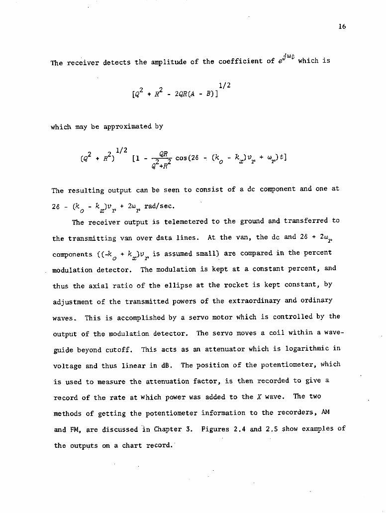
The receiver detects the amplitude of the coefficient of e6 a which is
[Q2 + R2 _ 2QR(A - B)]1/2
which may be approximated by
(Q2 + R2 1/2 [1 - 2 R2 cos(26 -(ko - k)v r + w r)t]Q +R
The resulting output can be seen to consist of a dc component and one at
26 - (k - k )vr + 2w rad/sec.
The receiver output is telemetered to the ground and transferred to
the transmitting van over data lines. At the van, the dc and 26 + 2wr
components ((-ko + kx)Vr is assumed small) are compared in the percent
modulation detector. The modulation is kept at a constant percent, and
thus the axial ratio of the ellipse at the rocket is kept constant, by
adjustment of the transmitted powers of the extraordinary and ordinary
waves. This is accomplished by a servo motor which is controlled by the
output of the modulation detector. The servo moves a coil within a wave-
guide beyond cutoff. This acts as an attenuator which is logarithmic in
voltage and thus linear in dB. The position of the potentiometer, which
is used to measure the attenuation factor, is then recorded to give a
record of the rate at which power was added to the X wave. The two
methods of getting the potentiometer information to the recorders, AM
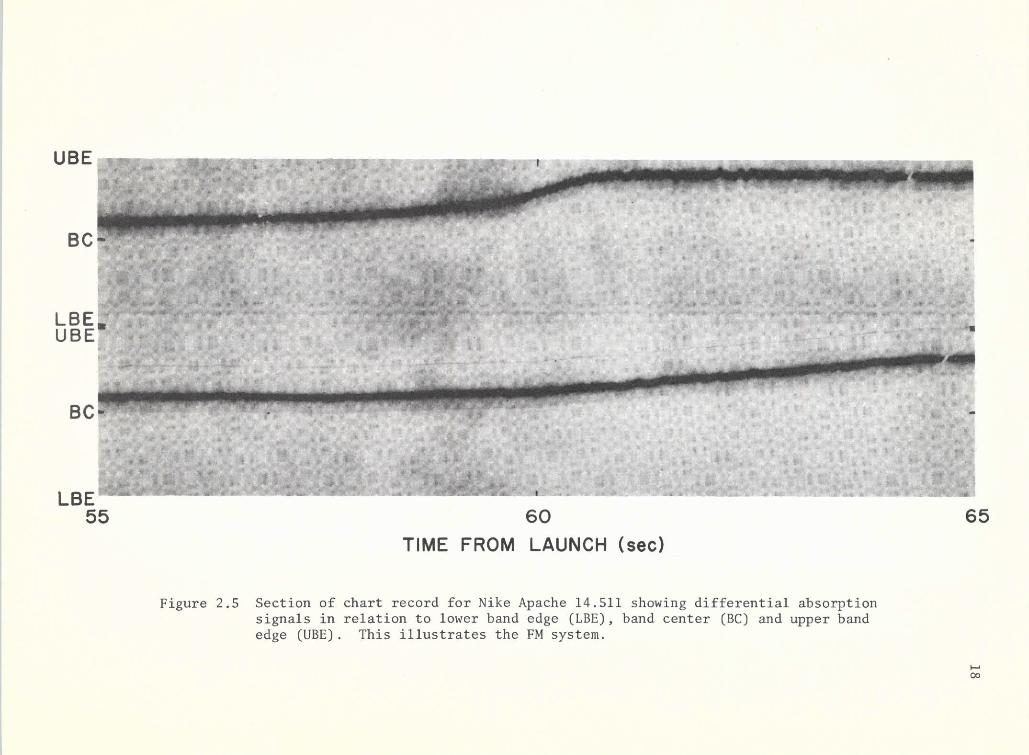
and FM, are discussed in Chapter 3. Figures 2.4 and 2.5 show examples of
the outputs on a chart record.

UBE
BC
LBE.UBE
BC
LBE 60 6555 60
TIME FROM LAUNCH (sec)
Figure 2.4 Section of chart record for Nike Apache 14.513 showing differential absorption
signals in relation to lower band edge (LBE), band center (BC) and upper band
edge (UBE). This illustrates the AM system.
.., .... ... ~-- - - -- - -~ - -- -~
UBE
BC-
LBE
55 60 65TIME FROM LAUNCH (sec)
Figure 2.5 Section of chart record for Nike Apache 14.511 showing differential absorptionsignals in relation to lower band edge (LBE), band center (BC) and upper bandedge (UBE). This illustrates the FM system.
o00
19
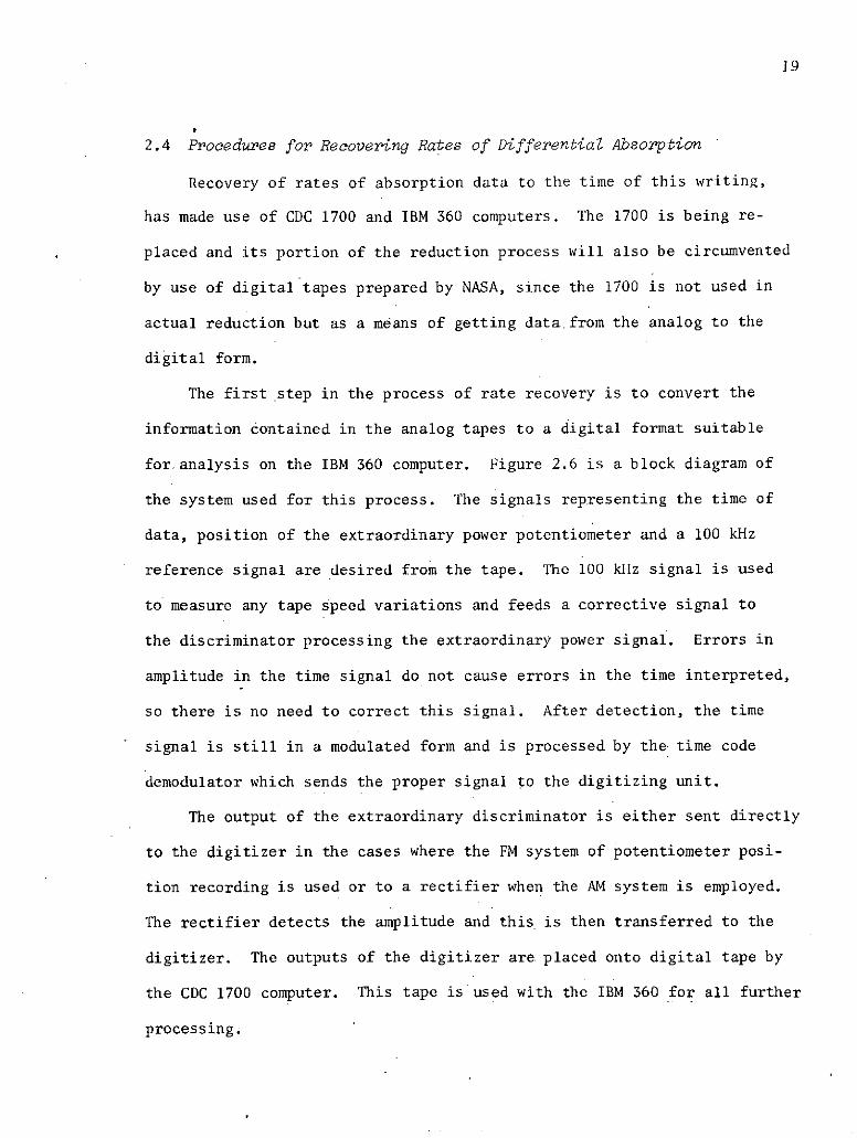
2.4 Procedures for Recovering Rates of Differential Absorption
Recovery of rates of absorption data to the time of this writing,
has made use of CDC 1700 and IBM 360 computers. The 1700 is being re-
placed and its portion of the reduction process will also be circumvented
by use of digital tapes prepared by NASA, since the 1700 is not used in
actual reduction but as a means of getting data from the analog to the
digital form.
The first step in the process of rate recovery is to convert the
information contained in the analog tapes to a digital format suitable
for analysis on the IBM 360 computer. Figure 2.6 is a block diagram of
the system used for this process. The signals representing the time of
data, position of the extraordinary power potentiometer and a 100 kHz
reference signal are desired from the tape. The 100 kHz signal is used
to measure any tape speed variations and feeds a corrective signal to
the discriminator processing the extraordinary power signal. Errors in
amplitude in the time signal do not cause errors in the time interpreted,
so there is no need to correct this signal. After detection, the time
signal is still in a modulated form and is processed by the time code
demodulator which sends the proper signal to the digitizing unit.
The output of the extraordinary discriminator is either sent directly
to the digitizer in the cases where the FM system of potentiometer posi-
tion recording is used or to a rectifier when the AM system is employed.
The rectifier detects the amplitude and this is then transferred to the
digitizer. The outputs of the digitizer are placed onto digital tape by
the CDC 1700 computer. This tape is used with the IBM 360 for all further
processing.

DISCRIMINATOR
.0 TIME MDISCRIMINATOR
TAPE PLAYBACK
TIME CODE
CDC IDEMODULATOR
1700 DIGITIZER
< RECTIFIER
Figure 2.6 Block diagram of digitizing process.
0

21
On the 360, DACAL is run first. It processes the data from the pre-
flight calibrations to determine which signal levels correspond to given
attenuator settings.
The final step of recovering the rates of absorption is accom-
plished through program DAPROC. This program analyzes the data on the
tape and gives an output of rates of differential absorption in dB/sec.
The program may also be directed to punch cards with the differential
absorption rates and complete trajectory data for the rocket. This is
needed as input for the program which analyzes the data to determine
electron concentrations.
2.4.1 Computer determination of electron concentration from dif-
ferential absorption rates. Mechtly et al. [1967] discuss the evalua-
tion of electron concentrations when Faraday rotation data are available.
We will deal here with the evaluation of these data in the absence of
Faraday rotation.
If the rocket trajectory and the characteristic of the magnetic
field are known the only unknown in the equations for determining how
each mode is absorbed are collision frequency and electron concentration.
To solve for the electron concentration, a model for the collision fre-
quency must be used. It is assumed that the collision frequency is pro-
portional to pressure.
Vm = C x 10 5 p(z) (2.25)
The problem of determining C is discussed by MechtZy [1974].

22
With the value of C chosen, and given pressures taken from
1972, the necessary information to solve for the electron density is
at hand. The program assumes an initial electron density and then
applies the exact form of the Sen-Wyller equations to determine a dif-
ferential absorption rate. This is compared with the measured rate and
the assumed electron density modified. This process is repeated six
times after which it usually has converged to within better than one
percent.

23
3. IMPROVEMENTS MADE IN DATA ACQUISITION AND REDUCTION SYSTEMS
As stated in the Introduction, one of the objectives of this project
was to find ways to improve the data, specifically at low altitudes. In
an effort to improve the operation of the data acquisition and reduction
systems, several of the components making up the differential absorption
experiment have been improved. This chapter will examine why the AM data
link was replaced by the new FM system and the resulting improvement.
Then the operation of tape speed compensation will be reviewed and its
effects on the data discussed. Finally the possible use of filtering to
recover data from the AM system will be reviewed.
3.1 FM Data System
3.1.1 Theoretical superiority of frequency over amplitude modula-
tion as a data link. Part of the original equipment in the University of
Illinois van consisted of an amplitude modulated link to transmit the
information about the attenuator position to the recording station.
This system, shown in Figure 3.1, simply generated a signal with an
amplitude proportional to the attenuator position. Due to age, the per-
formance of the four oscillators was degraded and replacements became
necessary. With the necessity of replacement, the possible use of a fre-
quency modulated system was examined to see if improvement could be
made.
For transmission systems, the figure of merit may be used as a
basis of comparison. The figure of merit is defined as the signal-to-
noise ratio out of a receiver, divided by the signal-to-noise ratio of
the incoming signal,

MATCHING MATCHINGTRANSFORMER TRANSFORME
AUDIO OSC FREQ. A95 Hz . X POWER DATA LINE
145 Hz FREQ.ASPOWERE
gX POWER t
O POWER
Figure 3.1 Block diagram of amplitude modulated data link.

25
So °o (3.1)
iM
with NM being the noise power within the receiver bandwidth.
For an AM system with a signal Am(t) cos2fo t, y was found by Taub
and Schilling [1971] to be
t= m2 ) (3.2)
1 + m2 t)
where m (t) is the mean square value of the modulation coefficient.
For the period of the flight when the differential absorption is
just beginning, the signal can be approximated by a sinusoid of ampli-
tude C leading to a figure of merit
C2
YAM - 2 (3.3)2 + C
For an FM system under the influence of a sinusoid, Taub and
Schilling show that
3 2YB (3.4)
B is the modulation index for the FM signal, f/fM fm being the maximum
frequency deviation. Since the same potentiometers would be used in
the FM system it will have the same modulation index as the AM system,
B = C. With this

26
3 C2 (3.5)SFM 2
To compare the two systems the ratio of their figures of merit will be
used
3 22 (2 + C2) = 3 + 3 C2 (3.6)yFM 2 3 2 2
YAM C2 2
2 + C2
This indicated that the implementation of an FM system will improve the
noise rejection of the data transfer process by more than three.
Because of this result, an FM link was installed.
3.1.2 Design of frequency modulated data link. Figure 3.2 shows
how the FM system was implemented. To minimize alterations to the sys-
tem, as few changes as possible were introduced. In place of the four
audio oscillators of the AM system, a single precision dc supply was
installed. The voltages present at the variable contacts of the poten-
tiometers are then used as the inputs to voltage controlled oscillators.
To choose the VCO frequencies, tests were run on the data lines at
Wallops Island, Virginia, to determine their frequency response charac-
teristics. Figure 3.3 gives the frequency responses of four data lines
and the locations of IRIG proportional bandwidth channels 1 through 10.
It is desirable to use the highest useful frequencies since the data
rate increases with the higher channels. Under these restrictions,
channels 4 through 7 were selected.

A ' VCO AMPLIFIER LI NE RECORDER
. POWEI
SYSTEMB
X POWER VCO
SYSTEM
L AVCOO POWER
Figure 3.2 Block diagram of frequency modulated data link.

<tol IRIG CHANNELS: WW 8 9 jZ-
10-2 I , , I I I i i
10 102 103 104
FREQUENCY (Hz)
Figure 3.3 Measured frequency response of four data lines at Wallops Island, 0shown in relation to IRIG channels 1 to 10.

29
3.1.3 Data reduction with frequency modulated system. As noted in
Chapter 2, with the addition of the FM system, the process of digitiza-
tion is simplified since the additional rectifier in Figure 2.6 is no
longer required. The change from the AM to the FM system, however,
revealed an inefficiency in the .median value subroutine of DAPROC.
When 14.511, the first rocket launch during which the FM system was
used, was processed it took DAPROC four minutes of IBM 360 computer time
to analyze 4 seconds of data, where previously up to 40 seconds had been
processed when the AM system was employed. To show how this happened,
Figures 3.4 and 3.5 show how samples of data for both the AM and FM sys-
tem might look. The noise present in the AM system is a function of
two factors: 1) increase noise in data transfer, and 2) incomplete
filtering of the carrier signal by the rectifier.
If the signal has no noise and the curve is monotonically increas-
ing, the median value will be located at the mid-point on the time axis
of the period of interest. With the noisy data, the routine would find
the median in a reasonable time because a point of magnitude equal to
the median is found early in the data. If the data are smooth, as that
generated by the FM system, the routine will search through nearly
half the data to get to the median. With 10,000 data points, this means
5,000 passes through the data making comparisons, or 5 x 10⁷ comparisons.
To rectify the problem, the statement directly above 200 in DAPROC,
Figure 3.6, is changed to Test = XPWR(ISTOP/2), moving the initial
search point to the mid-point of the time slot. With this change,
DAPROC was able to process 40 seconds of data from 14.511 in less than
three minutes.

30
Z0
RECTIFIED OUTPUTOF AM SYSTEM
O FIRST DATA = MEDIANa-
w "REAL DATA
MEDIAN POINT
TIME
Figure 3.4 Possible AM system data.

31
zO
DATA FROM FM
0 FIRST DATA = MEDAN
O "REAL" DATA
Lr MEDIAN POINTU-)
TIME
Figure 3.5 Possible FM system data.

32START
IT STOP=I STOP+1
NN2 =I STOP/2
MN= I
TEST =xPWP(1)
NLT O=0NGT =0NEQ =0K=MN
> 0 PWR(K) <0
=0
NGT= NEQ = NLT=NGT+I1 NEQ +1 NLT+1
XPGT.(NGT) XPLT (NLT)=XPWR(K) =XPWR (K)
NO KZ
Figure 3.6 Flowchart of original DAPROC program. This flow-chart is a corrected version of that given by
-Slekys and Mechtly [1970]. The program listingin that reference is correct and is currentlystored on the IBM 360.

33
NGTT=NGT+T -NEQ
NGTP =NGTT
NGTT YES CALL=NN2 ' CONVRT
NONGTT =
N
GTTGENDNGTT +i GT+
IISTOP JNO NGT YES , I STOP=NLT = NGT
MN=2 MN = 2
TEST= TEST =X PLT(i) X PGT(1)
K=2 K=2
XPWR ( K)= XPWR (K)=XPLT(K) XPGT (K)
gNO K YES YES K NOKI K * K=K+1I STO I STOP
Figure 3.6 Continued

34
3.1.4 Verification of data link improvement by use of FM system. As
a means of testing the improvement made by using the FM system, data,
digitized while the potentiometers at the University of Illinois van were
locked, were analyze'd as if it represented real data. Table 3.1 lists the
rates of differential absorption that resulted from noise in the systems.
(During this test tape speed compensation discussed later was employed.)
The standard error of the FM system is .006 dB/sec with a maximum change
of .01 dB, the minimum change the programs are designed to measure. The
older AM system showed a larger .037 dB/sec standard with errors up to
.09 dB/sec possible.
As a result of the FM system, the data transfer can be eliminated
as a factor in the overall noise of the measurements involved in the
differential absorption experiment.
3.2 Effects of Tape Speed Variation on Data and its Correction
Figure 3.7 shows a chart record of the output of a discriminator
after being passed through a low pass filter of 10 Hz to remove the
real data, which are on a carrier at 145 Hz. What this signal repre-
sents is tape speed noise caused by flutter in the tape playback system.
In the analysis of data one second of data at a time has been used in
most cases. If the tape speed noise is assumed periodic, the worst case
occurs when one second of data corresponds to a multiple of the period
of the noise plus a half period,
1 sec = NT + T/2

35
TABLE 3.1
Test of Data Transfer System
Referenced D.A. Rate in dB/secTime AM system FM system
1 -.02 0
2 -.09 -.01
3 -.04 0
4 0 .01
5 .02 0
6 0 0
7 .02 0
8 0 0
9 0 0
10 -.04 0
11 .07 0
12 .02 0
13 -.02 -.01
14 0 .01
15 0
16 .01
17 -.01

0.2
O-J-0. I
>-0.2
0 2 3 4 5 6 7 8 9 10TIME (sec)
Figure 3.7 Tape Speed Error.

37
Under this condition, the total error caused by a signal of frequency f
and amplitude A is
AError -
in the one second of data. Since two adjacent seconds are used to com-
pute differential absorption rates and their errors will be in opposite
directions, the error in measurement will amount to
AError .
The noise in Figure 3.7 was found to have a primary frequency of
about 3.5 Hz and amplitude of .4 dB, so the resulting error would be
.02 dB.
3.2.1 Implementation of tape speed compensation. In order to
compensate for variation in the speed of tape passing through the play-
back system, tape speed compensation was implemented. TSC operates
by recording a 100 KHz signal onto the data tape at the same time the
data are recorded. During playback, this signal is fed into a reference
discriminator centered at 100 KHz. The output of the discriminator is
proportional to the difference between 100 KHz and the frequency of the
signal from the tape.
The signal to be digitized is passed through a delay line and then
into the discriminator. The delay line compensates for the time it takes
the 100 KHz signal to be processed in the reference discriminator. The

38
normal output of the discriminator is then added to the signal from the
reference. The resulting signal will have noise due to the tape speed
variation reduced by 30 dB.
3.2.2 Effectiveness of tape speed compensation in reducing noise.
To see what kind of improvement tape speed compensation would make,
flight 14.514 was reprocessed both with and without TSC. Table 3.2
shows the results of these runs. The standard correction is ±.015 dB/
sec. For a correction of this order, the 30 dB noise reduction of the
TSC system is sufficient to reduce tape speed noise below the levels
measurable by the programs.
3.3 Filtering of Signals to be Processed from AM System to Improve Data
Another test performed, to improve the quality of data processed
for flights employing the AM system, involved the use of filtering. A
bandpass filter is placed between the discriminator output and the
rectifier in Figure 2.6. The filter will remove noise that is not
associated with the data signal, such as dc offset noise. The results
of this test for flight 14.361 are shown in Table 3.3. The correction
has a standard value of .02 dB/sec. This is a small error relative to
those seen in the data, and thus does not warrant reprocessing of
older flights.
3.4 Results of Improvements
All of the new techniques discussed in this chapter have contributed
in some way to the more exact evaluation of data, but none accounts for
the large discrepancies noted in Chapter 1. Possible explanations for
the larger errors are covered in the following chapter, along with
errors that do not affectdata at low altitudes but become important
higher up in the ionosphere.

39
TABLE 3.2
Test of Tape Speed Compensation on Data
from 14.514
Differential Absorption Rates (dB/sec)TIME no Difference
after launch TSC TSC TSC - no TSC
40 0 0 041 0 .02 .0242 -.11 -.11 043 .08 .07 -.0144 .05 .05 045 0 .02 .02
46 -.15 -.16 -.0147 .10 .10 048 .13 .13 049 -.05 -.03 .0250 .11 .11 0
51 .02 0 -.0252 .02 .03 .0153 0 0 054 .59 .57 -.0255 .16 .16 0
56 .72 .70 -.0257 1.12 1.16 -.0458 1.25 1.25 059 2.34 2.33 -.0160 3.09 3.09 0
61 2.86 2.88 .0262 2.67 ;2.68 .0163 2.49 2.53 .0464 2.23 2.22 -.0165 1.36 1.36 0
66 1.42 1.41 -.0167 1.64 1.65 .0168 1.45 1.44 -.0169 1.13 1.12 -.0170 -.02 -.03 -.01
71 -.08 -.06 .0272 .32 .29 -.0373 -.11 -.01 .0274 .94 .92 -.0275 1.02 1.01 -.01

40
TABLE 3.3
Filter Test on 14.361
Differential Absorption RatesTime (dB/sec)
after launch No Filter Filter Change
48 .16 .20 -.04
49 .48 .46 .02
50 -.11 -.11 0
51 -.36 -.37 .01
52 .40 .42 -.02
53 .39 .37 .02
54 -.28 -.28 0

41
4. ERRORS IN THE SIGNAL RECEIVED BY TIIE ROCKET
This chapter will deal with errors not connected with the processing
or recording of data, but with errors at the rocket itself. The first
two sections present a more detailed analysis of the electric field than
has previously been undertaken and shows some faults in the experimental
assumptions. The last section deals with actual errors in the receiving
system itself.
4.1 Theory of Polarization Errors
The type of signals which can be expected from errors in the pol-
arization, those due to imperfect generation of the extraordinary and
ordinary modes, are examined. The wave form detected by the receiver
was derived as follows.
Two signal components are considered to be present at the frequency
w - 6. They are the ordinary wave,
i Q sin[(w-6)t - KooZ] - j Q cos[(w-6)t - KooZ]
and the unwanted extraordinary wave,
i S sin[(w-6)t - K Z] + j cos[(w-6)t - K oZ]
At the frequency w + 6 there are also two components present. The
extraordinary wave is represented as
iR sin[(m+6)t - K Z] + j R cos[(w+6)t - K Z]

42
and an unwanted ordinary wave is
i P sin[(w+6)t - KoxZ] - j P cos[(m+6)t - KoxZ]
The unit vector for the antenna is taken as in Chapter 2 to be
A A *
a = -i sinw t + j cosw t (4.1)
and the displacement is taken as
Z = vRt (4.2)
K 0 , K , K , and K represent the propagation constants. The first
subscript represents the mode of the wave, o for ordinary and x for
extraordinary. The second subscript is the frequency of operation, o
for the correct ordinary-frequency (w-6), and x for the correct extra-
ordinary frequency (w+6). vr is again the rocket velocity and wr the
spin rate of the rocket.
The signal received, represented as E * a is
-[Q sin(w-6-K oov r)t + S sin(w-6-K ov r)t
+ R sin(w+6-K V r)t + P sin(w+6-Kox v r)t] sinw rt
+ [-Q cos(w-6-K oo )t + S cos(w-6-K v )to r o - P osr
+ R cos(w+6-K v )t - P cos(w+6-K v )t] cosw t
43
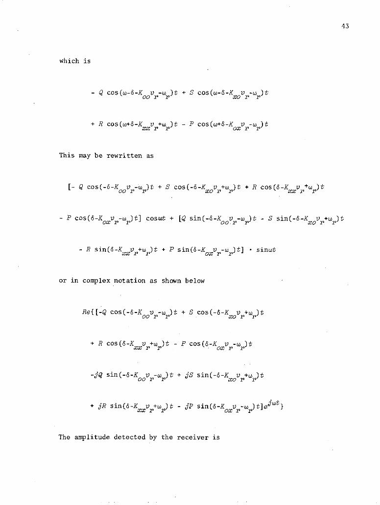
which is
- Q cos(w-6-K oovr- )t + S cos(w-6-K vr-r )t
+ R cos(m+6-Kx v r+r )t - P cos(m+6-K ox -wr )t
This may be rewritten as
[- Q cos(-6-K oov r-r )t + S cos(-6-K xor +wr)t + R cos(6-K v r+w r)t
- P cos(6-K v r-mr)t] coswt + [Q sin(-6-K v -wr)t - S sin(-6-K vr+w )t
- R sin(6-Kxx +w )t + P sin(-K xVr -w )t] sinwtr r oxr r
or in complex notation as shown below
Re{[-Q cos(-6-K oo r- r )t + S cos(-6-K o v r+ )t
+ R cos(6-Kxx v r+wr)t - P cos(6-K ox -wr)t
-jQ sin(-6-K oov r-r)t + jS sin(-6-K xo r+w r)t
+ jR sin(6-K v +w )t - jP sin(6-K v -W )t]eJwt}The amplitude detected by ther r oxr r
The amplitude detected by the receiver is

44
2 2 2 2 1/2{Q2 + S2 + R2 + P2 _ 2QS cos[-(K oo-K x)v - 2wr]t
-2QR cos[-26-(K o-K =)v r - 2w ]t + 2QP cos[-26-(K o-Kx ) r]t
(4.3)
+2SR cos[-26-(K o-K )v ]t + 2SP cos[-26-(K o-Kox ) r + 2w ]t
1/2-2RP cos[(K -Kox ) r + 2 w ]t}
The relation
1/2 X(1 + X) = 1 +
for X small may be used to reduce expression (4.3). Table 4.1 lists the
resulting frequencies and their proportional amplitudes.
Each frequency can be given a physical interpretation to help under-
stand what errors are occurring. Frequency b at 26 + 2wr is the fre-
quency discussed in Chapter 2. Frequencies a and f are caused by the
error signals at each transmitted frequency combining with the correct
signal to form a small linear signal. The linear signal's received
strength is then dependent on the antenna orientation and is therefore
modulated at 2w . Frequencies c and d are both caused by signals of
the same polarization, but different transmitter frequencies. Since
they are the addition of two circular modes in the same direction, they
result in a circular mode and are unaffected by rocket spin. The 26 is
caused by the envelope generated by the difference in frequency.

45
TABLE 4.1
Received Frequencies Including Polarization Errors
a (K o-K ) + 2w 2w QS2 + X r r
b 26 + (K oo-Kxx) r + 2wr 26 +2wr R
c 26 + (K oo-Kox )r 26 QP
d 26 + (K -Kx )v 26 SR
e 26 + (K xo-K ) -2 r 26 -2w SP
f (K xx-Kox ) + 2 2wr RP
S de Ip22 2 +R2 +S2 1/2

46
Frequency e is generated as in Chapter 2 but since the ordinary wave is
-now higher in frequency, the ellipse rotates opposite to the direction
in Chapter 2 and the rocket spin thus subtracts from the total. The
dc signal is the average signal strength present at the rocket.
4.2 Effect of Polarization Errors on System Response
Figures 4.1, 4.2, and 4.3 show the probe current and DA determined
electron concentrations. Note that in all cases the DA data from the
2.225 MHz system indicate low electron densities above 80 km. To see
if this could be due to polarization errors, a.Fourier.transform pro-
gram developed by K. L. Miller [Ediards, 1973] was used to recover the
power in the frequency components at 26, 26 + 2wr and 2wr . These powers
are shown in Figures 4.4 to 4.6. To see what has happened, it is
assumed that the error extraordinary signal is negligible; thus, S = 0
in Table 4.1. The amplitude of the ordinary error signal, P, may not be
assumed to be O since as the extraordinary wave is absorbed the power to
the extraordinary transmitter is increased, and thus the power in the
error wave, P. As the ratio of ordinary to extraordinary is being kept
constant, the magnitude of the error ordinary signal continues to in-
crease. At some point the magnitude of the error ordinary wave and the
extraordinary wave at the rocket are equal. At this point, the servo
system will follow the 26 rad/sec signal generated by the two ordinary
modes rather than the correct 26 + 2wr rad/sec signal. Appreciable de-
gradation of data is noted to occur when the 26 rad/sec signal power
reaches about one-fifth the magnitude of the 26 + 2r rad/sec component.
To get a measure of how much useful data can be extracted from a flight,
the powers of the 26 and 26 + 2wr components at low altitudes can be

PROBE CURRENT (A)1-8 C 1 1-6 Q -5
110
NIKE APACHE 14.511
-PROBE CURRENT100- a 2.225 MHz D.A.
A 3.385 MHz D.A. aC 7.3 x 10⁵
90-
E
80
H70
-J3
60
5 0 . 1 f il l I I I I lI[ Il I I I I I I Il I I I 1 1 1 110 102 103 104 105
ELECTRON DENSITY (cm 3 )
Figure 4.1 Profiles of probe current (upper scale) and electron density (lowerscale). Data from the differential absorption experiment aloneare shown.

PROBE CURRENT (A)10- 8 10- 7 -6 10- 5
1101
NIKE APACHE 14.513-- PROBE CURRENT
100 - o 2.225 MHz DA Aa 5.040 MHz DA
105 "AC= 7.3 x 10A "
90- A
E
< 70-
60- a3
D
50
10 10 z 103 104 105
-j3
ELECTRON DENSITY (cm 3 )
Figure 4.2 Profiles of probe current (upper scale) and electron density (lower scale).Data from the differential absorption experiment alone are shown.

PROBE CURRENT (A)-8 107 -6 1-5
110
NIKE APACHE 14.514
-PROBE CURRENT100- u 2.225 MHz DA
A 5.040 MHz DA A
C=7.3 X 10⁵
90
EE
80- 0W
- 70
60-
50- 1 1
10 102 103 104 105
ELECTRON DENSITY (cm-3)
Figure 4.3 Profiles of probe current (upper scale) and electron density (lower scale).Data from the differential absorption experiment alone are shown.

108
28 + 20r NIKE APACHE 14.511
V
10 74-
S "I
3 IL
LaI 2Wr /
ot .
0.eS"' f , "' \ i
28 \ / ,1/
10 , , , I
50 60 70 78
TIME FROM LAUNCH (sec)
Figure 4.4 Frequency components at receiver output.

51
10 I I-1
NIKE APACHE 14.513
-Q
IO I A'
50 60 70
TIME FROM LAUNCH (sec)
Figure 4.5 Frequency components at receiver output.

52
to
NIKE APACHE 14.514
28+2wr
IO7
. 28
S0 l I /
50 60 70
TIME FROM LAUNCH (sec)
Figure 4.6 Frequency components at receiver output.

53
compared. The difference in power in decibles minus seven decibles gives
the total range of useful absorption, the sum of the rates for each
second. Table 4.2 lists the power differences and useful data range
for 14.511, 14.513, and 14.514 and the second of flight and altitude
where the limit is passed.
4.3 Reflected Waves
The following will give an idea of the error to be expected when
reflections are present. The reflection coefficients for the extra-
ordinary and ordinary waves, as measured from the rocket, may be repre-
sented as r and F . Since the reflection coefficients are measuredx o
from the rocket, they include absorption over the path of the reflected
wave. The propagation will be along a magnetic field line so that the
mode of the reflected wave is the same as that of the incident wave.
The error in polarization is assumed to be zero.
The total electric field may be calculated as the sum of four
propagation vectors. First there are the two upward propagating modes
iQ sin[(w-6)t - KZ] - jQ cos[(w-6)t - KZ]
and
iR sin[(w+6)t - KZ] + jR cos[(w-6)t - KZ]
where it is now assumed for simplicity that the propagation constant,
K, is the same for both modes. The two reflected vectors can be repre-
sented as
iQro sin[(w-6)t + KZ] - jQro cos[(w-6)t + KZ]

54
TABLE 4.2
Power Differences, Useful Data Range, and Limit
of Data in Time and Altitude for Three Rocket Flights
Difference Useful Last Useful DataFlight Power (dB) Range (dB) Time (sec) Altitude (km)
14.511 20 13 59 75
14.514 19 12 61 75
14.513 19 11 59 75

55
and iRo sin[(w+6)t + KZ] + jRFx cos[(-r6)t + KZ].
By going through the procedure of Section 4.1 the amplitude of the
signal detected by the receiver is
{[1 + o2]Q2 + [1 + x 2 ] R2 - 2QR cos(26 + 2wr)t
+ 2Q2r cos(2Kv r)t - 2QRI x cos[26 + 2Kv + 2w r )t
2QRFo cos(26 - 2Kv + 2 w )t
1/2+ 2R 2F cos(2Kv r)t - 2QRT F cos(26 + 2w )t}
x r ox r
If r and r are small and R is much less than Q the expansion usedX o
in Section 4.1 is valid and the amplitude and frequencies present in the
output are shown in Table 4.3. Thus, under the conditions of reflected
waves with absorption the modulation index, M, is
QR(1 + rot )M = 2 2 2 2 1/2 (4.4)
[(1 + r ) + (1 + )R] (4.4)o X
It can be seen that changes in the shape of the ionosphere above the
rocket will cause the index M to change and the system to wander looking
for a proper setting to hold M constant, as shown in Figure 4.7.
When perfect reflections'occur the expansion used breaks down. To
examine this case let R = 0, so that only the ordinary wave is present,
and let F = -1. The receiver output is then0

56
TABLE 4.3
Frequencies in Receiver Output when Reflections are Present
for r F << 1 and R << Q
Frequency Amplitude
dc [(1+2 )Q2 + (1+r2 )R 1/2oQ R2
2Kv r Q2 + R2
26 + 2w QR + rr xQR
26 + 2wr + 2Kvr xQR
26 + 2w - 2Kv r' R

UBE
LBEC
UBE
LBE95 100 105
TIME FROM LAUNCH (sec)
Figure 4.7 Section of chart record for Nike Apache 14.520 showing differential absorptionsignals in relation to lower band edge (LBE), band center (BC) and upper bandedge (UBE). This is the FM system used for a nighttime flight.
- -------- U,

58
[2Q - 2Q 2 cos(2KVrt)]1 /2
This can be rewritten as
2Q1 sin(Kvrt)I
The frequencies in the output are shown in Table 4.4. Note that the dc
term is larger than that for only an upward traveling ordinary wave when
it would be simply Q.
It should be noted that this analysis does not hold near the ordinary
reflection point the wave is no longer circular, but linear. Also the
reflection occurs at X = 1 due to ray bending.
To connect the results of sections one to three of this chapter
Figure 4.8 shows the output spectrum of the receiver during flight 14.270.
All of the frequency components around 500 Hz predicted are present.
4.4 Receivers
Another source of errors in the experiment is the noise picked up
by the receivers. Figure 4.9 shows the noise temperature, a measure of
the amount of noise present, as a function of frequency. As can be seen,
the frequencies used by the experiment, 2.225 KHz, 3.385 KHz, and
5040 KHz, are in a portion of the spectrum with highly variable noise
characteristics. The following is a calculation of the signal-to-noise
ratio at the rocket for the 2.225 KHz system.
The loss of signal due to the length of the propagating path for an
isotropic radiator is

59
TABLE 4.4
Receiver Output for r =-l and R = 0
Frequency Component Altitude
4&dc
4&r 3T
4Kv 4Qr 157-
2nKv 4Qr (4n2 - 1)

60
7 IIT 'I
28+2r6
5 DATA INTERVAL74.5 -75.5 sec
4w0-
2 2(+w +(r +oUdr)
2(8+w,+u,)-2(_8- w ) 28
480 490 500 510 520 530 540 550FREQUENCY (Hz)
Figure 4.8 Frequency spectrum of receiver output signalfor Nike Apache 14.270, prepared by K. L.Miller [Edwards, 1973].

61
10'" ----
Max.
1012 ---
& 101 -
to
c Cosmic106 Ato iconoise
10,
Sto 2I II i I I I I --
I I
10--
CL
C-
0.1 0.5 1.0 5 10 50 100
Frequency - MHzFigure 4.9 Noise temperature at medium and high
frequencies [Jordan and Balmain, 1968].

62
L = 10 log h (4.5)
under the assumption of no absorption. If the rocket is at 100 km, the
loss is 50 dB at 2.225 KHz. The transmitter power (PT) is originally
about 5 watts for the extraordinary signal which is 7 dBw. The combined
gains of the antennas (G) are about 2 dB. The resulting signal power at
the rocket is then
PR = PT + G - L (4.6)
which is -41 dB in this case.
The total noise power received is
N = K' + T + B (4.7)
in which K' is 10 log k (Boltzmann's constant), equal to -229 dBw/OK Hz,
T is 10 log Ta (noise temperature) and B is 10 log BW (bandwidth). For
a good payload receiver, BW is 1500 Hz. The temperatures chosen from
Figure 4.10 are about 1000 K at minimum and 1010K at maximum. These
result in a maximum noise power of -100 dB and a minimum of -180 dB.
Comparing the signal power to the noise power, the signal-to-noise
ratios of 139 dB and 59 dB result. Clearly random atmospheric noise is
not an important factor over the 30 dB range of absorption the experi-
ment is designed to operate over.
In addition to random atmospheric noise the signal may include
unwanted radiofrequency transmissions. The receiver's bandpass

63
characteristic is poor in this respect. Examination of bandpass curves
of receivers used in the payload shows a slow falloff and extraneous
peaks. This can become important when the frequencies of the experi-
ment are not far removed from those used by others. 2225 KHz is
located in a frequency range used for radiotelegraph and ship-to-shore
communications. Both of the upper frequencies used are within the
tropical broadcast bands, used by countries near the equator because of
poor propagation at normal broadcast band frequencies, as listed in
Tables 4.5 and 4.6. Part of the hazard presented by these other users
can be reduced by monitoring the receiver output prior to launch with
the transmitters momentarily shut off. If there are any strong signals
present, the rocket should not be launched unless poor performance of
the differential absorption experiment is risked.
Another area in which other users of the airways may present a
problem occurs because the receivers, when placed in a payload, receive
signals at frequencies other than those for which they are designed.
Table 4.7 shows the location of peaks outside the passband and the
amount of attenuation at these points. It must be pointed out that
this is not a particularly bad receiver and that all units tested
showed this type of response. The frequency locations of these peaks
do vary between receivers. Several of these fall in the broadcast band
and if there is a nearby station it could affect data. This problem
will show itself, if the above test for other stationsnear the operation
frequency is done.

64
TABLE 4.5
Stations Near 3.385 MHzPower
Frequency in Kilowatts Country
3380 18 Mali
100 Malawi
1 Guatamala
.25 Bolivia
1 Peru
3385 .075 Indonesia
.3 Indonesia
10 Sri Lanka
.6 New Guinea
4 Dominican Republic
1 Brazil
1 Peru
1 Venezuela
3390 10 Afghanistan
120 China
.2 Panama
.25 Bolivia
5 Ecuador
.3 Peru

65
TABLE 4.6
Stations Near 5.040 MHz
Frequency Power Country
5037 1 Angola
50 USSR
30 Central African Rep.
1 Brazil
1 Columbia
5 Ecuador
.5, 1 Peru
5038 30 Central African Rep.
5039 20 Sudan
5040 50 USSR
50 Burma
none given China
.05 Indonesia
.15 Haiti
1 Ecuador
10, .5 Peru
1 Venezuela
5041 10 Guinea
1 Phillipines
1 Cook Islands
5 Bolivia
1 Brazil
1 Peru

66
TABLE 4.7
Extra Signals Detected by
Receiver #106 in 5040 Payload
Frequency Attenuation
556 -26 dB
585 -52 dB
601 -52 dB
635 -52 dB
674 -52 dB
695 -52 dB
741 -30 dB
856 -46 dB
927 -47 dB
1112 -23 dB
1236 -47 dB
1309 -43 dB
1483 -34 dB
1853 -42 dB
2780 -38 dB
3177 -28 dB
3705 -54 dB
4449 -20 dB

67
5. RANGE AND ACCURACY OF DIFFERENTIAL ABSORPTION DATA
In view of what has been discussed in the previous chapters about
errors, it is appropriate to define a basis upon which the useful range
of data may be determined. Chapter 4, Section 2, established an upper
limit on the experiment, as a result of the polarization error. Here the
lower limit of useful data will be fixed and some discussion of the
accuracy of the measurements will be undertaken. For this purpose, Tables
5.1 to 5.3 present a summary of the results of the rate recovery program
for three flights.
5.1 Lower Limit of Differential Absorption Data
The problem is to estimate the lowest differential absorption rate
which can be considered to be a significant measure of real absorption.
To get a measure of the random errors, several seconds of data are
processed before absorption starts. This is then used to compute the
standard error of measurement. Table 5.4 shows the errors for the
flights under discussion. The criteria for determining the starting
point for good data is to select the first data point greater than the
standard error after which there are two or more data points also
greater than the standard error. This point up to where polarization
error takes over is the range of useful data.
Figures 5.1 to 5.3 show the probe current and only the useful dif-
ferential data set by the procedures above and in Chapter 4. The
polarization was not checked for the higher frequency in each experiment
so the cutoff is taken as the first data point of value less than the
standard error.

68
TABLE 5.1
14.511 - 2.225 and 3.385 KHzDifferential Absorption Rates
Time 2.225 rate 3.385 rateafter launch (dB/sec) (dB/sec)
49 .07 .0450 .05 -.1951 .13 .2752 .25 .2753 .27 -.2654 .27 .3655 .33 .4556 .60 .0457 .96 -.3558 1.79 .8959 3.06 .9260 8.49 2.0761 2.39 2.7562 .22 2.2563 2.7864 2.5665 .7366 .9167 1.2668 1.1269 .6270 1.4271 .0272 1.3173 1.7374 2.1075 -1.1676 1.3477 .3078 -.4679 .6280 .11

69
TABLE 5.2
14.513 - 2.225 and 5.04 MHzDifferential Absorption Rates
Time 2.225 MHz 5.04 MHz
after launch (dB/sec) (dB/sec)
40 .1241 .1042 .0443 -.0844 .0245 .1046 -.0447 -.0448 .2049 .0250 .12 .1851 .36 .18
52 .44 -.71
53 -.12 .37
54 .58 -.16
55 .74 -.0556 1.04 .27
57 1.56 .1658 2.96 .38
59 2.84 .07
60 3.70 -.05
61 3.21 .49
62 2.53 .02
63 2.10 .18
64 1.73 .22
65 .79 -.02
66 .42 -.05
67 .26 .75
68 .07 -.51
69 .07 .42
70 .31 .33
71 .52 -.18
72 .57 .58
73 .83 .47
74 .87 .3775 .47
76 1.30
77 .84
78 .8279 1.57
80 13.75
81 -.6882 1.33

70
TABLE 5.2
14.513 - 2.225 and 5.04 MHz (cont.)
Time 2.225 MHz 5.04 MHz'after launch (dB/sec) (dB/sec)
83 .1284 -.2085 -.2786 -.88,87 4.5688 -1.2589 1.7590 -2.58

71
TABLE 5.3
14.514 - 2.225 and 5.04 MHz
Differential Absorption Rates
Time 2.225 MHz 5.04 MHz(dB/sec) (dB/sec)
42 -.1143 .0744 .0545 .0246 -.1647 .1048 .1349 -.0350 .11 -.0551 0 .0252 .03 .4753 0 -.. 4654 .57 -.2055 .16 -.0756 .70 .3857 1.16 .2458 1.25 .0259 2.33 -.1560 3.09 .0761 2.88 .4662 2.68 .1163 2.53 .3664 2.22 -.0265 1.36 -.1166 1.41 -.0967 1.65 .2668 1.44 .1569 1.12 070 -.03 .2271 -.06 1.1172 .29 -.3173 -.09 .58
74 .92 .2675 1.01 .5176 .71 .6477 0 - .4678 0 .4679 0 25.58

72
TABLE 5.4
Lower Limit of Data
Standard First Significant DataFlight Frequency Error Time from Altitude
(dB/sec) Launch (sec) (km)
14.511 2.225 .07 51 61
3.385 .29 58 74
14.513 2.225 .16 54 65
5.04 .33 72 91
14.514 2.225 .09 73 65
5.04 .26 73 92

PROBE CURRENT (A)
10-8 IO- 7 I0 - 6 10- 5
110 lcFI
NIKE APACHE 14.511
SPROBE CURRENT100- a 2.225 MHz DA
A 3.385 MHz DA A
C=7.3x 10pA
90
CJ
6O
60 -
500I0 102 103 104 105
ELECTRON DENSITY (cm-3 )
Figure 5.1 Profiles of probe current (upper scale) and electron density
(lower scale).

PROBE CURRENT (A)10- 10- 7 10-6 10-5
110
NIKE APACHE 14.513- PROBE CURRENT
100- a 2.225 MHz DAa 5.040 MHz DA
C =7.3 x 10⁵p
90
w 80
70
60
50I I 1 iI I Ji lI I II
10 102 10 104 105
ELECTRON DENSITY (cm 3 )
Figure 5.2 Profiles of probe current (upper scale) and electron density(lower scale).

PROBE CURRENT (A)
10- 8 10 7 10-6 10-5
110
NIKE APACHE 14.514PROBE CURRENT
100 - a 2.225 MHz D.A.a 5.040MHz D.A.
C= 7.3 x 10⁵ p
90-
E
80H L
1 70
60
50 -10 102 103 . 104 105
ELECTRON DENSITY (cm -3 )
Figure 5.3 Profiles of probe current (upper scale) and electron density
(lower scale).

76
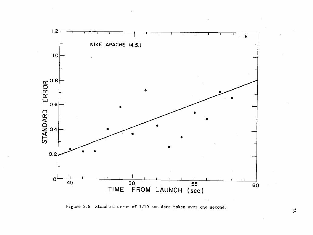
5.2 Error in CaZculated Electron Densities
The shaded area in Figure 5.4 shows the range over which the electron
densities for 14.511 can fall if the errors of up to the standard error in
Table 5.1 in the 2225 KHz system are allowed. As would be expected, as
the rocket goes further and the rate of absorption increases, the random
error represents a smaller portion of the total data. It will be shown
below that standard errors previously calculated are not valid above the
first few data points, but are a reasonable estimate. Figure 5.5 shows
the standard error of each second of data as calculated from the rates of
absorption taken one tenth of a second at a time. The magnitude of the
error is not in agreement with that calculated in the last section. The
reason for this is that the errors are not independent because of the
feedback in the system. If the servo moves too fast, resulting in a
high absorption rate being recorded, the feedback will result in some
data where the rate is slower as the servo returns to its proper
setting. The result is that the time over which data are averaged
affects the statistics in that the longer the time the more closely the
errors approximate independent random values. For this reason, the
error values in Figure 5.5 are of larger magnitude than when whole
seconds of data were taken at a time. To limit the effect of real ab-
sorption, the errors are calculated from a straight line fit of the
data generated for that second. Clearly the result shows that as the
rocket penetrates the ionosphere the errors increase. The error is
increasing at a rate near a factor of two for every ten kilometers of
ionosphere traveled through. If this factor is used starting from the
first valid point, the error range shown by the dotted line in Figure
5.4 results.

80 I 1 I I I i I
NIKE APACHE 14.511C 3.88X 10⁵ p
70
H -*
7- 2
60I0 10 103
ELECTRON DENSITY (cm 2 )
Figure 5.4 Estimated error in electron density.
1.2 I I
NIKE APACHE 14.511
1.0-
0.8
0*
w 00.6-
Z 0.4 - *
I- *(,)
0.2
045 50 55 60
TIME FROM LAUNCH (sec)
Figure 5.5 Standard error of 1/10 sec data taken over one second.00

79
5.3 Collision Frequency
Mechtly [1974] discussed the problem of analyzing differential ab-
sorption data in the absence of Faraday rotation. It will be recalled
that under these conditions a collision frequency model of the form
vm = C x 105p is used. Figure 5.6 shows the results of using C = 3.88
and C = 7.3 on the data from 14.511. Looking at Figure 2.1 one notices
that using the Sen-Wyller formulation, the absorption is nearly inde-
pendent of collision frequency at 72 km. This is confirmed by the
crossing of the two curves in Figure 5.6 near this altitude.
At points where the data starts, near 62 km, the error between the
curves resulting from the choice of C, is greater than that due to
inaccuracy in the measurement of the absorption rates.. One point that
should be noted is that at the 72 km point both errors in measurement
and of collision frequency selection are only a small fraction of the
total electron concentration. This means that if the probe experiments
electron concentration to current ratio is constant in the lower iono-
sphere the 72 km point becomes an excellent calibration point.

80 I 1 1 1 I I I I
NIKE APACHE 14.511
0 C= 3.88 XI0 5 p
© C=7.3 X 10⁵p
E- 70 1
F-2
_J
60 1
I0 10 " 103
ELECTRON DENSITY (cm 3 )
Figure 5.6 Electron densities using different collision frequency models.
o0

81
6. CONCLUSIONS AND RECOMMENDATIONS
6.1 Areas of Experiments Usefulness
As a result of careful examination of experimental equipment and pro-
cedures, it is felt that the objective of improving the experiment to a
-3point where electron concentrations on the order of 10 cm-3 are measured,
is not obtainable, without major system changes. The level to which the
experiment can be used is a function of the absorption the wave goes
through. 14.511 which was launched on a day of high absorption allowed
the experiment to be used down to about 100 cm- 3 . The other day shots
examined, 14.513 and 14.514, for which the absorption was not as high,
were useful to levels of 200 cm- 3 . For nighttime shots with little
absorption, the experiment is generally rendered useless by reflections.
As a result of the analysis of where the data can be used, the
2.225 MHz system is found to be useful in the day generally only between
65 and 75 kilometers. The use of the 5.04 MHz system is useful only over
an area of about five kilometers. The 3.385 MHz, not generally used in
the day, is found to work reasonably well giving much more information
than available from the 5.04 MHz system.
6.2 System Change Recommendations
The following are suggestions for changes in the system which will
lead to improved operation of the differential absorption experiment.
None of these changes will degrade the operation of the Faraday rotation
experiment.
6.2.1 Polarization. To stop the servo system from following the 26
signal generated by the error signals, filters can be employed. Two

82
possibilities exist., A notch filter set to eliminate any signal at 26 can
be used, or a bandpass filter centered at 26 + 2w with enough attenuation
at 26 to effectively make it 0. For either system, the filter would have
to be bypassed for ground tests and during early stages of flight before
the spin rate becomes appreciable. The bandpass filter has a disadvantage
in that different characteristics would be needed for rockets using dif-
ferent spin rates. The filter must be of very narrow characteristics in a
slow spin rocket since it would be desirable to have 40 dB of attenuation
in, the 26 signal only 2Wr radians/sec away from the center of the pass-
band. Some of the bandpass filter's faults could be overcome by the use
of a tracking filter which will follow the signal as the spin rate
changes. These could be set at 26 at launch and would then follow the
signal as the spin rate builds. up, providing constant system lock.
For the notch filter only one need be designed centered at 26. It
should provide 20 dB of attenuation at 26 and essentially none at 26 + 2w
when the smallest spin rate is present in the area of data considered.
In addition to filtering to separate the 26 and 26 + 2wr signals, an
improved filter to separate the dc component is needed. The servo has
been noted to follow the 2wr modulation present. The present filter is a
first order filter at 1 Hz. It would be desirable to replace this by one
with an upper 3 dB point at 2 Hz and with attenuation of.40 dB at about
8 Hz. This dc filter would most likely improve the standard error of
the measurements.
It may be advisable to change the value of 6, which is now 250 Hz,
if a filter is used. By changing 6 down to 50 the Q's of the filter

83
sections can be reduced by a factor of 5 making stability of the filter
less of a problem. This would require, however, redesign of the modula-
tion detector.
Another approach to the problem is to improve the actual polarization
characteristics. This is not deemed practical, as an improvement of a
factor of about 50 would be needed. This type of improvement could not
be obtained with a simple antenna system required for field operation.
6.2.2 Receivers.: As noted in Chapter 4 the receivers have many
undesirable characteristics. These characteristics have been worse in
the newer receivers. Since the receivers were originally designed in
the early 60's many improvements in techniques have been made. It is
suggested that new receivers be designed. These new receivers need not
be as sensitive as those presently used. Any sensitivity beyond that
necessary to detect the propagating wave, after going through 30 dB of
attenuation, will only result in increased noise pickup.
6.3 Data Reduction
Most of the improvements in this area are under way. The data now
comes digitized on tapes, eliminating that step in the processing. What
needs to be done now is to streamline the processing by reducing the
amount of human data handling. A start in this area is being made by
having each program punch its results onto cards with the appropriate
data for the next step. The goal should be to design the processing so
that two sets of cards are generated, one with differential absorption
data and trajectory, and the other with Faraday rotation data and tra-
jectory. These could then be used in a single program to generate elec-
tron densities.

84
6.4 Further Test Suggestions
The effect the telemetry system has on the accuracy of the experiment
was not studied. It would be desirable to make a few tests while the
rocket is on the ground to measure the accuracy of the telemetry system.
One test would be to operate all systems as if under flight conditions
and record the servo systems movements. This will test the noise gener-
ated by the transmitter to rocket to telemetry station to van loop.
Next simulate the expected receiver output at the VCO's in the payload
to eliminate the transmitter to rocket section of the loop. Finally,
simulate the expected inputs to the data lines at the telemetry station
to test the line and the modulation measuring equipment in the van.
If the test of the loop shows errors in recording on the order of
.07 dB/sec when analyzed as real data, the loop may be the source of
most of the experiment's errors. The further tests will help evaluate
where the most improvement can be made.

85
REFERENCES
Appleton, E. V. (1932), Wireless studies of the ionosphere, J. Instn. Elec.
Engrs. 71, 642-650.
Edwards, B. (1973), Research in Aeronomy: October 1, 1972-March 31, 1973,
Prog. Rep. 73-1, Aeron. Lab., Dep. Elec. Eng., Univ. Ill., Urbana-
Champaign.
Hartree, D. R. (1931). The propagation of electro-magfetic waves in a
refracting medium in a magnetic field, Proc. Cambridge Phil. Soc. 27,
143-162.
Jordan, E. C. and K. G. Balmain (1968), Electromagnetic Waves and Radiating
Systems, Prentice-Hall, Inc., Englewood Cliffs, New Jersey.
Knoebel, H., D. Skaperdas, J. Gooch, B. Kirkwood, and H. Krone (1965),
High resolution radio frequency measurements of Faraday rotation
and differential absorption with rocket probes, Coord. Sci. Lab.
Rep. R-273, Univ. Ill., Urbana-Champaign.
Mechtly, E. A., S. A. Bowhill, L. G. Smith, and H. Knoebel (1967), Lower
ionosphere electron concentration and collision frequency from rocket
measurements of Faraday rotation, differential absorption, and probe
current, J. Geophys. Res. 72, 5239.
Mechtly, E. A. (1974), Accuracy of rocket measurements of lower ionosphere
electron concentrations, Radio Sci. 9, 373-378.
Salah, J. E., and S. A. Bowhill (1966), Collision frequencies and electron
temperatures in the lower ionosphere, Aeron. Rep. No. 14, Aeron. Lab.,
Dep. Elec. Eng., Univ. Ill., Urbana-Champaign.
Sen, H. K., and A. A. Wyller (1960), On the generalization of the Appleton-
Hartree magnetoionic formulas, J. Geophys. Res. 65, 3931-3950.

86
Slekys, A. G., and E. A. Mechtly (1970), Aeronomy Laboratory system for
digital processing of rocket telemetry tapes, Aeron. Rep. No. 35,
Aeron. Lab., Dep. Elec. Eng., Univ. Ill., Urbana-Champaign.
Taub, H., and R. L. Schilling (1971), Principles of Communication Systems,
McGraw-Hill, Inc., New York, 268-319.


