

A.I. in health informatics lecture 3 clinical reasoning & probabilistic inference, II*
kevin small & byron wallace
*Slides borrow heavily from Andrew Moore, Weng-‐Keen Wong and Longin Jan Latecki

today
• probabilistic reasoning – Bayesian networks – reasoning with uncertainty – crucial building block for automated clinical
reasoning systems
• review conditional independence and (a little) graph theory

introduction
• diagnosing inhalational anthrax
• observe the following symptoms – patient has difficulty breathing – patient has a cough – patient has a fever – patient has diarrhea – patient has inflamed mediastinum

introduction
• diagnoses often stated in probabilities (e.g. 30% chance of inhalational anthrax)
• additional evidence should change your degree of belief in the diagnosis
• how much evidence until absolutely certain?
• Bayesian networks are a methodology for reasoning with uncertainty

review: random variables
• basic element of probabilisAc reasoning
• refers to an event drawn from a distribuAon modeling the uncertain outcome of the event

Boolean random variables
• takes the values true or false
• can be thought of event occurred or event didn’t occur
• examples notation – patient has inhalational anthrax A – patient has difficulty breathing B – patient has a cough C – patient has a fever F – patient has diarrhea D – patient has inflamed mediastinum M

joint probability distribution
• expresses probability between arbitrary number of variables
• for each combinaAon, states how probable said combinaAon is
A D M P(A,D,M)
false false false 0.65
false false true 0.03
false true false 0.1
false true true 0.04
true false false 0.02
true false true 0.06
true true false 0.03
true true true 0.07
must sum to 1
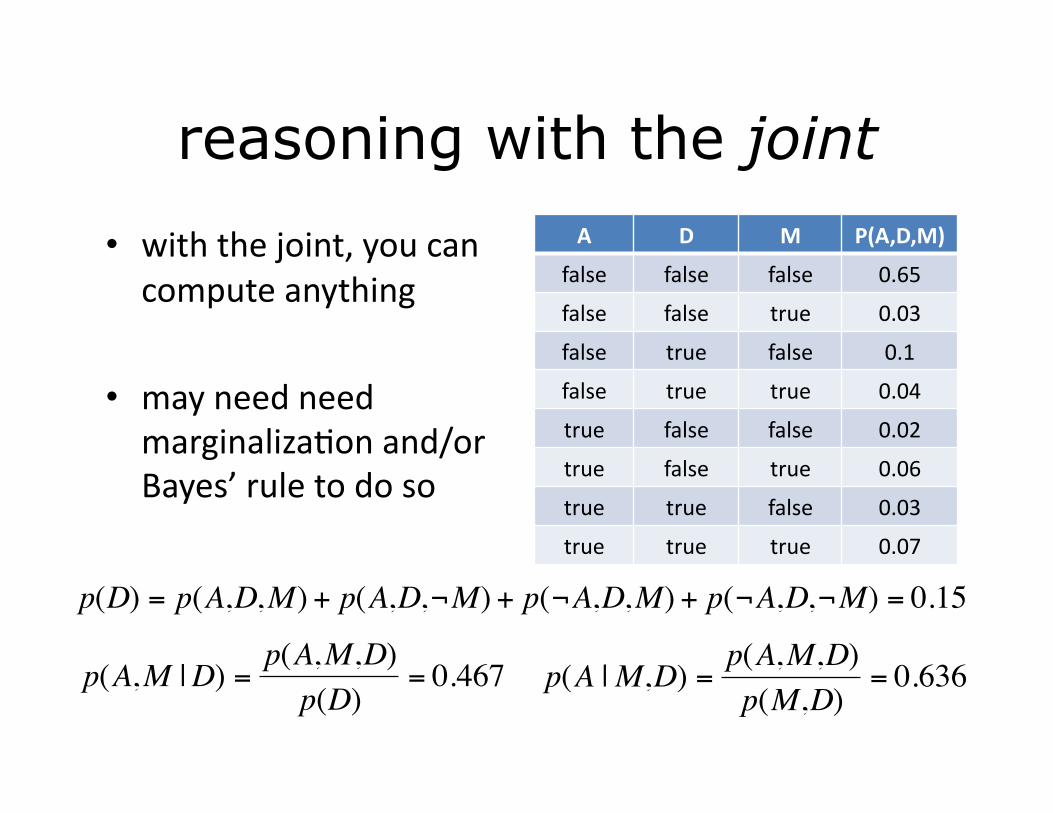
reasoning with the joint
• with the joint, you can compute anything
• may need need marginalizaAon and/or Bayes’ rule to do so
A D M P(A,D,M)
false false false 0.65
false false true 0.03
false true false 0.1
false true true 0.04
true false false 0.02
true false true 0.06
true true false 0.03
true true true 0.07
€
p(D) = p(A,D,M) + p(A,D,¬M) + p(¬A,D,M) + p(¬A,D,¬M) = 0.15
€
p(A,M |D) =p(A,M,D)p(D)
= 0.467
€
p(A |M,D) =p(A,M,D)p(M,D)
= 0.636

problems with the joint
• not a compact representaAon – requires 2n-‐1 parameters to express
– requires a lot of data to accurately esAmate
• (condiAonal) independence to the rescue!

independence
• random variables A and B are independent if – p(A,B) = p(A) p(B) – p(A|B) = p(A) – p(B|A) = p(B)
knowledge regarding outcome of A provides no addiAonal informaAon about the outcome of B

independence
• independence allows compact representaAon
• suppose n coin flips – joint requires 2n-‐1 parameters – if flips independent, requires n parameters

conditional independence
• random variables A and B are condiAonally independent if – p(A,B|C) = p(A|C) p(B|C) – p(A|B,C) = p(A|C) – p(B|A,C) = p(B|C)
knowledge regarding outcome of A provides no addiAonal informaAon about the outcome of B

Bayesian networks (finally!)
• a Bayesian network G=(V,E) is composed of – a directed acyclic graph – a set of condiAonal probability tables (CPT)
A
B
C D
B D P(D|B)
false false 0.02
false true 0.98
true false 0.05
true true 0.95
A B P(B|A)
false false 0.01
false true 0.99
true false 0.7
true true 0.3
B C P(C|B)
false false 0.4
false true 0.6
true false 0.9
true true 0.1
A P(A)
false 0.6
true 0.4

semantics of structure
A
B
C D
A P(A)
false 0.6
true 0.4
each vertex is a random variable
B is a parent of D; D is condiAoned on B
B D P(D|B)
false false 0.02
false true 0.98
true false 0.05
true true 0.95
each vertex has CPT p(Xi|Parents(Xi))

• a Boolean variable with n parents has 2n+1 entries (2n which must be stored)
• note what must sum to 1
conditional probability tables
A
B
A
B
E A B P(B|A)
false false 0.01
false true 0.99
true false 0.7
true true 0.3
A B E P(B|A,E)
false false false 0.2
false false true 0.1
false true false 0.8
false true true 0.9
true false false 0.25
true false true 0.98
true true false 0.75
true true true 0.02

utility of Bayes nets
• two important properAes – encodes condiAonal independence relaAonships between random variables in the graph
– compact representaAon of the joint
X
P1 P2
C1 C2
ND2 ND1
given parents (P1,P2), a vertex X is condiAonally independent of its non-‐descendents (ND1,ND2)

calculating the joint
• can compute joint using Markov condiAon
€
p(A,B,¬C,D) = p(A)⋅ p(B | A)⋅ p(¬C |B)⋅ p(D |B)
€
p X1 = x1,…,Xn = xn( ) = p Xi = xi |Parents Xi( )( )i=1
n
∏
A
B
C D €
= 0.4⋅ 0.3⋅ 0.9⋅ 0.95 = 0.1026

inference
• compuAng probabiliAes specified by model
• generally queries of the form
€
p(X | E)
A
B
C D
evidence variable(s) query variable(s)

inference
• compuAng probabiliAes specified by model
• let’s try
€
p(C | A)
A
B
C D
evidence variable(s) query variable(s)
to the board!

bad news
• exact inference is feasible in only small to medium sized networks
• exact inference in larger networks takes a long Ame
• can use approximate inference

network structure
• use domain expert knowledge to design
• learn it from data – not trivial
• good news is clinical experAse is high
A
B
C D

naïve Bayes
• another opAon is to make strong (condiAonal) independence assumpAons
• ogen effecAve for classificaAon models
A
B C D F M
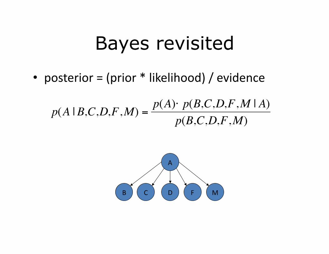
Bayes revisited
• posterior = (prior * likelihood) / evidence
€
p(A |B,C,D,F,M) =p(A)⋅ p(B,C,D,F,M | A)
p(B,C,D,F,M)
A
B C D F M

conditional independence
• assume input variables condiAonally indendent
A
B C D F M
€
p(A | X) =
p(A)⋅ p Xi | A( )i=1
n
∏p(X)
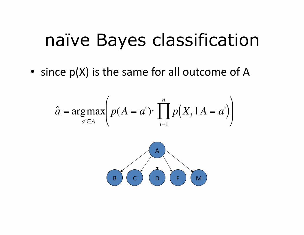
naïve Bayes classification
• since p(X) is the same for all outcome of A
€
ˆ a = argmaxa '∈A
p(A = a')⋅ p Xi | A = a'( )i=1
n
∏⎛
⎝ ⎜
⎞
⎠ ⎟
A
B C D F M

number of parameters
• joint probability distribuAon
• naïve Bayes
• inference runAme
• to esAmate parameters, count (and smooth)
€
O n A( )€
2n −1 = 63
€
A −1+ A Xi −1( ) =11i=1
n
∑

example day outlook temperature humidity wind tennis
1 sunny hot high weak no
2 sunny hot high strong no
3 overcast hot high weak yes
4 rain mild high weak yes
5 rain cool normal weak yes
6 rain cool normal strong no
7 overcast cool normal strong yes
8 sunny mild high weak no
9 sunny cool normal weak yes
10 rain mild normal weak yes
11 sunny mild normal strong yes
12 overcast mild high strong yes
13 overcast hot normal weak yes
14 rain mild high strong no
Given today is sunny, cool but windy with high humidity, will we play tennis?
[Mitchell’s Machine Learning Book]
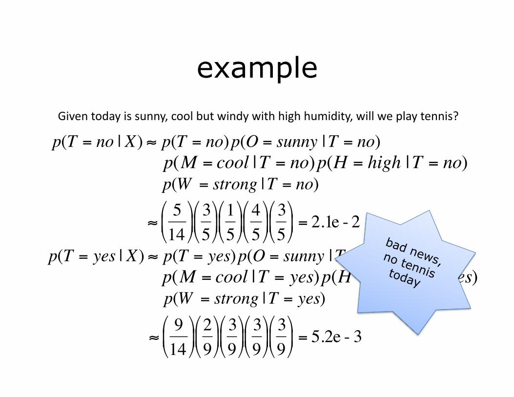
example Given today is sunny, cool but windy with high humidity, will we play tennis?
€
p(T = no | X) ≈ p(T = no)p(O = sunny |T = no)
€
p(M = cool |T = no)p(H = high |T = no)
€
p(W = strong |T = no)
€
p(T = yes | X) ≈ p(T = yes)p(O = sunny |T = yes)
€
p(M = cool |T = yes)p(H = high |T = yes)
€
p(W = strong |T = yes)
€
≈914⎛
⎝ ⎜
⎞
⎠ ⎟ 29⎛
⎝ ⎜ ⎞
⎠ ⎟ 39⎛
⎝ ⎜ ⎞
⎠ ⎟ 39⎛
⎝ ⎜ ⎞
⎠ ⎟ 39⎛
⎝ ⎜ ⎞
⎠ ⎟ = 5.2e - 3
€
≈514⎛
⎝ ⎜
⎞
⎠ ⎟ 35⎛
⎝ ⎜ ⎞
⎠ ⎟ 15⎛
⎝ ⎜ ⎞
⎠ ⎟ 45⎛
⎝ ⎜ ⎞
⎠ ⎟ 35⎛
⎝ ⎜ ⎞
⎠ ⎟ = 2.1e - 2

PopulaAon-‐wide ANomaly DetecAon and Assessment (PANDA)
• a detector for a large-‐scale outdoor release of inhalaAonal anthrax
• massive Bayes net
• populaAon-‐wide means each person has their own subnetwork in the model
[Wong et al., KDD 2005]

population-wide approach
• anthrax is non-‐contagious – reflected in network structure
Time of Release
Person Model
Anthrax Release
Location of Release
Person Model Person Model

person model Anthrax Release
Location of Release Time Of Release
Anthrax Infection
Home Zip
Respiratory from Anthrax
Other ED Disease
Gender Age Decile
Respiratory CC From Other
Respiratory CC
Respiratory CC When Admitted
ED Admit from Anthrax
ED Admit from Other
ED Admission
Anthrax Infection
Home Zip
Respiratory from Anthrax
Other ED Disease
Gender Age Decile
Respiratory CC From Other
Respiratory CC
Respiratory CC When Admitted
ED Admit from Anthrax
ED Admit from Other
ED Admission
… …
Yesterday never
False
15213
20-30 Female
Unknown
15146
50-60 Male

advanced topics
• learning network structure – generally a search procedure
• Markov networks – considers undirected edges
• influence diagrams – generalized with determinisAc verAces
• more inference – variable eliminaAon, approximate inference

more?
current standard bearer
the classic
really interesAng


