

Algorithmics - Lecture 2 1
LECTURE 2:
Algorithms
pseudocode; examples

Algorithmics - Lecture 2 2
Organizational:
Webpage: up and running.
Newsgroup: algouvt on yahoo groups. Please subscribe.
First homework: posted tomorrow on the webpage.
DEADLINE (firm): Friday, October 19, 5pm.

Algorithmics - Lecture 2 3
Outline
• Continue with algorithms/pseudocode from last time. • Describe some simple algorithms
• Decomposing problems in subproblems and algorithms in subalgorithms

Algorithms - Lecture 1 4
Properties an algorithm should have
• Generality
• Finiteness
• Non-ambiguity
• Efficiency
Algorithms - Lecture 1 5
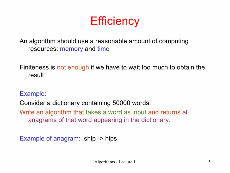
Efficiency
An algorithm should use a reasonable amount of computing resources: memory and time
Finiteness is not enough if we have to wait too much to obtain the result
Example:
Consider a dictionary containing 50000 words.
Write an algorithm that takes a word as input and returns all anagrams of that word appearing in the dictionary.
Example of anagram: ship -> hips

Algorithms - Lecture 1 6
EfficiencyFirst approach:
Step 1: generate all anagrams of the word Step 2: for each anagram search for it in the dictionary (using
binary search)
Let’s consider that:– the dictionary contains n words – the analyzed word contains m letters
Rough estimate of the number of basic operations:– number of anagrams: m!– words comparisons for each anagram: log2n (e.g. binary search)
– letters comparisons for each word: m
m!* m*log2n

Algorithms - Lecture 1 7
EfficiencySecond approach:
Step 1: sort the letters of the initial word Step 2: for each word in the dictionary having m letters:
• Sort the letters of this word• Compare the sorted version of the word with the sorted version
of the original word
Rough estimate of the number of basic operations:– Sorting the initial word needs almost m2 operations (e.g. insertion
sort)
– Sequentially searching the dictionary and sorting each word of length m needs at most nm2 comparisons
– Comparing the sorted words requires at most nm comparisons
n m2 +nm+ m2

Algorithms - Lecture 1 8
Efficiency
First approach Second approach
m! m log2n n m2 +n m+ m2
Example: m=12 (e.g. word algorithmics) n=50000 (number of words in dictionary) 8* 10^10 8*10^6 one basic operation (e.g.comparison)= 1ms=10-3 s24000 hours 2 hours
Thus, important to analyze efficiency and choose more efficient algorithms
Which approach is better ?

Algorithms - Lecture 1 9
Outline
• Problem solving
• What is an algorithm ?
• Properties an algorithm should have
• Describing Algorithms
• Types of data to use
• Basic operations

Algorithms - Lecture 1 10
How can we describe algorithms ?
Solving problems can usually be described in mathematical language
Not always adequate to describe algorithms because:
– Operations which seem elementary when described in a mathematical language are not elementary when they have to be encoded in a programming language
Example: computing a sum, computing the value of a polynomial
∑i=1
n
i=1+2+ . ..+n
Mathematical description Algorithmic description (it should be a sequence of basic operations)

Algorithms - Lecture 1 11
How can we describe algorithms ?
Two basic instruments:• Flowcharts:
– graphical description of the flow of processing steps– not used very often, somewhat old-fashioned. – however, sometimes useful to describe the overall structure of
an application• Pseudocode:
– artificial language based on• vocabulary (set of keywords)• syntax (set of rules used to construct the language’s
“phrases”)– not as restrictive as a programming language

Algorithms - Lecture 1 12
Why do we call it pseudocode ?
Because … • It is similar to a programming language (code)
• Not as rigorous as a programming language (pseudo)
In pseudocode the phrases are:
• Statements or instructions (used to describe processing steps)
• Declarations (used to specify the data)

Algorithms - Lecture 1 13
Types of dataData = container of information
Characteristics:– name
– value• constant (same value during the entire algorithm)• variable (the value varies during the algorithm)
– type• primitive (numbers, characters, truth values …)• structured (arrays)

Algorithms - Lecture 1 14
Types of data
Arrays - used to represent:• Sets (e.g. {3,7,4}={3,4,7})
– the order of the elements doesn’t matter
• Sequences (e.g. (3,7,4) is not (3,4,7))– the order of the elements matters
• Matrices – bidimensional arrays
7 34
1
0
0
1
3 7 4
Index: 1 2 3
1
10
0
(1,1) (1,2)
(2,1) (2,2)

Algorithms - Lecture 1 15
How can we specify data ?
• Simple data:
– Integers INTEGER <variable>
– Reals REAL <variable>
– Boolean BOOLEAN <variable>
– Characters CHAR <variable>

Algorithms - Lecture 1 16
How can we specify data ?
Arrays
One dimensional
<elements type> <name>[n1..n2]
(ex: REAL x[1..n])
Two-dimensional
<elements type> <name>[m1..m2, n1..n2]
(ex: INTEGER A[1..m,1..n])

Algorithms - Lecture 1 17
How can we specify data ?
Specifying elements:– One dimensional
x[i] - i is the element’s index
– Two-dimensional
A[i,j] - i is the row’s index, while j is the column’s index

Algorithms - Lecture 1 18
How can we specify data ?
Specifying subarrays:
• Subarray= contiguous portion of an array
– One dimensional: x[i1..i2] (1<=i1<i2<=n)
– Bi dimensional: A[i1..i2, j1..j2]
(1<=i1<i2<=m, 1<=j1<j2<=n)
1 ni2
i1
m
1
i2
1 n
j1 j2
i1

Algorithms - Lecture 1 19
Outline
• Problem solving
• What is an algorithm ?
• Properties an algorithm should have
• Describing Algorithms
• Types of data to use
• Basic instructions
Algorithms - Lecture 1 20
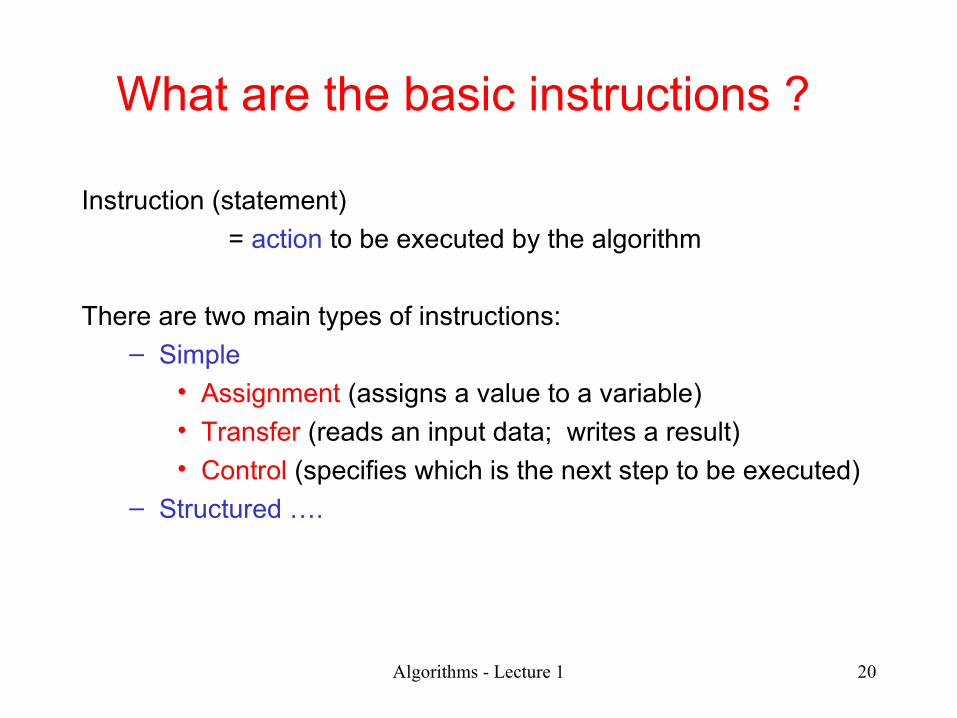
What are the basic instructions ?
Instruction (statement)
= action to be executed by the algorithm
There are two main types of instructions:– Simple
• Assignment (assigns a value to a variable)• Transfer (reads an input data; writes a result)• Control (specifies which is the next step to be executed)
– Structured ….

Algorithms - Lecture 1 21
• Aim: give a value to a variable• Description:
v ← <expression>
Rmk: sometimes we use := instead of ←
• Expression = syntactic construction used to describe a computation
It consists of:– Operands: variables, constant values– Operators: arithmetical, relational, logical
Assignment
Algorithms - Lecture 1 22
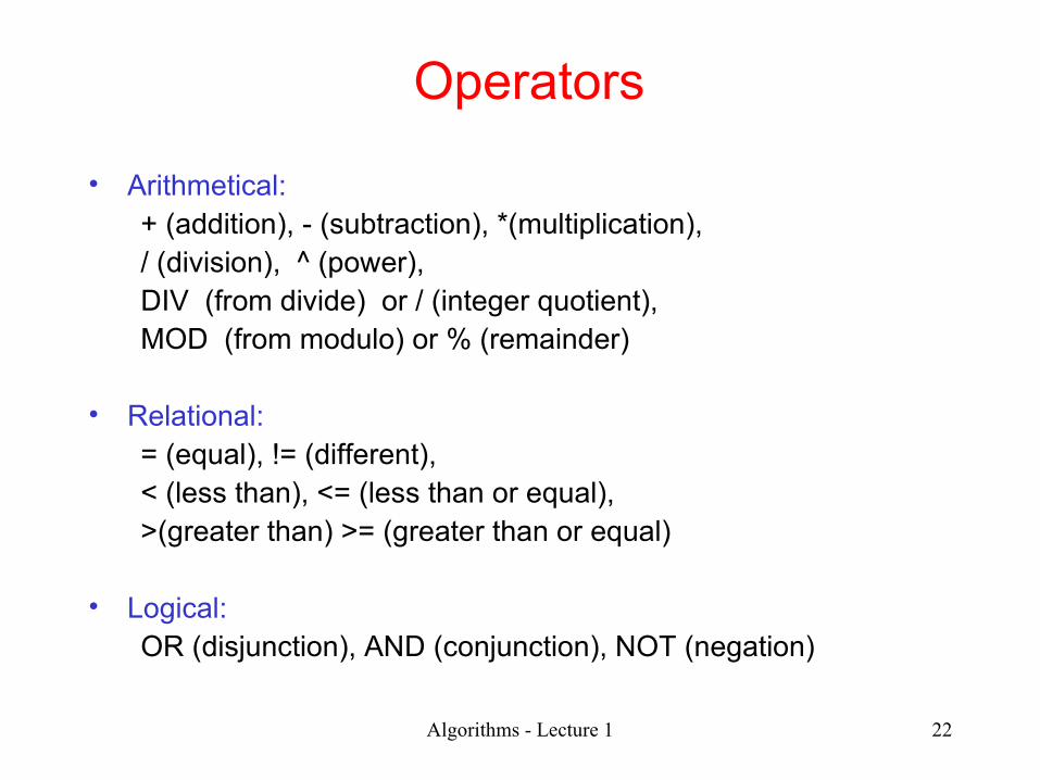
• Arithmetical:+ (addition), - (subtraction), *(multiplication), / (division), ^ (power), DIV (from divide) or / (integer quotient), MOD (from modulo) or % (remainder)
• Relational:= (equal), != (different), < (less than), <= (less than or equal),>(greater than) >= (greater than or equal)
• Logical: OR (disjunction), AND (conjunction), NOT (negation)
Operators

Algorithms - Lecture 1 23
Input/Output
• Aim: – read input data – output the results
• Description:
read v1,v2,… input v1, v2,…
write e1,e2,… print e1, e2,…
23
user userVariables of the algorithm
read (input)
write (print)
Input Output

Algorithms - Lecture 1 24
Instructions
Structured:– Sequence of instructions
– Conditional statement
– Loop statement

Algorithms - Lecture 1 25
condition
condition
<S1> <S2>
<S>
True False
True False
Conditional statement• Aim: choosing between two or several alternatives
depending on the value of some conditions
• General variant:
if <condition> then <S1> else <S2>endif
• Simplified variant:
if <condition> then <S>endif

Algorithms - Lecture 1 26
Loop statements
• Aim: repeating a processing step• Example: compute a sum
S= 1+2+…+i+…+n• Characterized by:
– Processing step which have to be repeated– Stopping (or continuation) condition
• Depending on the moment of analyzing the stopping condition there are two main loop statements:– Preconditioned loops (WHILE loops)– Postconditioned loops (REPEAT loops)

Algorithms - Lecture 1 27
<condition>
<statement>
Nextstatement
False
True
while <condition> do <statement>endwhile
WHILE loop• First, the condition is analyzed
• If it is true then the statement is executed and the condition is analyzed again
• If the condition becomes false the control of execution passes to the next statement in the algorithm
• If condition never becomes false then the loop is infinite
• If the condition is false from the beginning then the statement inside the loop is never executed

Algorithms - Lecture 1 28
<condition>
<statement>
Nextstatement
False
True
while <condition> do <statement>endwhile
WHILE loop
S:=0 // initialize the variable which will // contain the resulti:=1 // index intializationwhile i<=n do S:=S+i // add the current term to S i:=i+1 // prepare the next termendwhile
∑i=1
n
i=1+2+ . ..+n

Algorithms - Lecture 1 29
FOR loop
• Sometimes the number of repetitions of a processing step is known apriori
• Then we can use a counting variable which varies from an initial value to a final value using a step value
• Repetitions: v2-v1+1 if step=1
v <= v2
<statement>
Nextstatement
False
True
for v:=v1,v2,step do <statement>endfor
v:=v+step
v:=v1
v:=v1while v<=v2 do
<statement>v:=v+step
endwhile

Algorithms - Lecture 1 30
FOR loop
v <= v2
<statement>
Nextstatement
False
True
for v:=v1,v2,step do <statement>endfor
v:=v+step
v:=v1
S:=0 // initialize the variable which will // contain the result
for i:=1,n do S:=S+i // add the term to Sendfor
∑i=1
n
i=1+2+ . ..+n

Algorithms - Lecture 1 31
REPEAT loop
• First, the statement is executed. Thus it is executed at least once
• Then the condition is analyzed and if it is false the statement is executed again
• When the condition becomes true the control passes to the next statement of the algorithm
• If the condition doesn’t become true then the loop is infinite
<condition>
<statement>
Nextstatement
True
repeat <statement>until <condition>

Algorithms - Lecture 1 32
REPEAT loop
<condition>
<statement>
Nextstatement
True
repeat <statement>until <condition>
S:=0 i:=1repeat S:=S+i i:=i+1until i>n
∑i=1
n
i=1+2+ . ..+n
S:=0 i:=0repeat i:=i+1 S:=S+iuntil i>=n

Algorithms - Lecture 1 33
REPEAT loop
Any REPEAT loop can be transformed in a WHILE loop:
<statement>
while NOT <condition> DO
<statement>
endwhile
<condition>
<statement>
Nextstatement
True
repeat <statement>until <condition>

Algorithms - Lecture 1 34
Summary
• Algorithms are step-by-step procedures for problem solving
• They should have the following properties:•Generality•Finiteness•Non-ambiguity (rigorousness)•Efficiency
• Data processed by an algorithm can be • simple• structured (e.g. arrays)
•We describe algorithms by means of pseudocode
Algorithms - Lecture 1 35
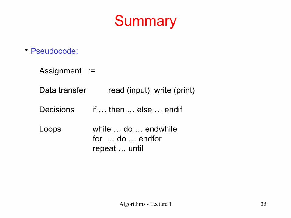
Summary
• Pseudocode:
Assignment :=
Data transfer read (input), write (print)
Decisions if … then … else … endif
Loops while … do … endwhile for … do … endfor repeat … until

Algorithmics - Lecture 2 36
Example 1Consider a table containing info about student results
No. Name Marks ECTS Status Average
1 A 8 6 7 60
2 B 10 10 10 60
3 C - 7 5 40
4 D 6 - - 20
5 E 8 7 9 60
Task: fill in the status and average fields such that
status = 1 if ECTS=60
status= 2 if ECTS belongs to [30,60)
status= 3 if ECTS<30
the average is computed only if ECTS=60

Algorithmics - Lecture 2 37
Example 1The filled table should look like this:
No. Name Marks ECTS Status Average
1 A 8 6 7 60 1 7
2 B 10 10 10 60 1 10
3 C - 7 5 40 2 -
4 D 6 - - 20 3 -
5 E 8 7 9 60 1 8
Algorithmics - Lecture 2 38
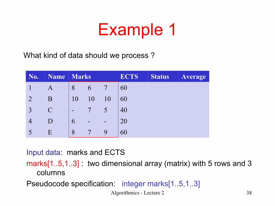
Example 1What kind of data should we process ?
No. Name Marks ECTS Status Average
1 A 8 6 7 60
2 B 10 10 10 60
3 C - 7 5 40
4 D 6 - - 20
5 E 8 7 9 60
Input data: marks and ECTS
marks[1..5,1..3] : two dimensional array (matrix) with 5 rows and 3 columns
Pseudocode specification: integer marks[1..5,1..3]
Algorithmics - Lecture 2 39
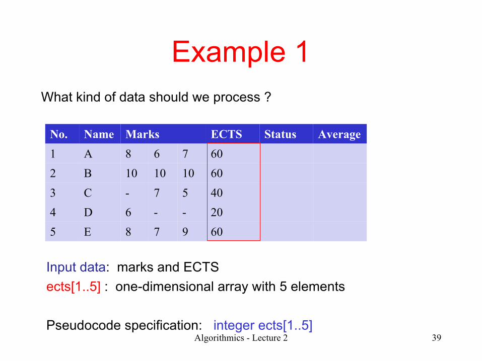
Example 1What kind of data should we process ?
No. Name Marks ECTS Status Average
1 A 8 6 7 60
2 B 10 10 10 60
3 C - 7 5 40
4 D 6 - - 20
5 E 8 7 9 60
Input data: marks and ECTS
ects[1..5] : one-dimensional array with 5 elements
Pseudocode specification: integer ects[1..5]

Algorithmics - Lecture 2 40
Example 1What kind of data should we process ?
No. Name Marks ECTS Status Average
1 A 8 6 7 60
2 B 10 10 10 60
3 C - 7 5 40
4 D 6 - - 20
5 E 8 7 9 60
Output data: status and average
status[1..5], average[1..5] : one-dimensional arrays with 5 elements
Pseudocode specification: integer status[1..5]
real average[1..5]

Algorithmics - Lecture 2 41
Example 1Rule to fill in the status of a student
status = 1 if ECTS=60
status= 2 if ECTS belongs to [30,60)
status= 3 if ECTS<30
ects=60
Pseudocode description:
if ects=60 then status←1
else if ects>=30 then status ← 2
else status ← 3
endif
endif
status ← 1
yes
ects>=30
status ← 2 status ← 3
no
noyes Python description
if ects==60:status=1
elif ects>=30:status=2
else:status=3

Algorithmics - Lecture 2
Example 1Filling in the status of all students: for
each student fill in the status field
Remark: Let us denote with n the number of students (in our example n=5)
Step 1: start from the first element (i:=1)
Step 2: check if there are still elements to process (i<=n); if not then STOP
Step 3: compute the status of element i
Step 4: prepare the index of the next element
Step 5: go to Step 2
compute status[i]
i ← 1
i<=n
i ← i+1
=60
1 >=30
2 3

Algorithmics - Lecture 2
Example 1Filling in the status of all
students: for each student fill in the status field
compute status[i]
i ← 1
i<=n
i ← i+1
Pseudocode:
integer ects[1..n], status[1..n], i
i ← 1
while i<=n do
if ects[i]=60 then status[i] ← 1
else if ects[i]>=30 then status[i] ← 2
else status[i] ← 3
endif
endif
i ← i+1
endwhile

Algorithmics - Lecture 2
Example 1Simplify the algorithm description by
grouping some computation in “subalgorithms”
Pseudocode:
integer ects[1..n], status[1..n], i
i ← 1
while i<=n do
status[i] ← compute(ects[i])
i ← i+1
endwhile
Subalgorithm (function) description:
compute (integer ects)
integer s
if ects=60 then s ← 1
else if ects>=30 then s ← 2
else s ← 3
endif
endif
return s
Remark: the subalgorithm describes a computation applied to generic data

Algorithmics - Lecture 2
Using subalgorithmsBasic ideas:
– Decompose the problem in subproblems
– Design for each subproblem an algorithm (called subalgorithm or module or function)
– The subalgorithm actions are applied to some generic data (called parameters) and to some additional data (called local variables)
– The execution of subalgorithm statements is ensured by calling the subalgorithm
– The effect of the subalgorithm consists of:• Returning some results• Modifying the values of some variables which are accessed
by the algorithm (global variables)

Using subalgorithmsThe communication mechanism between an algorithm and its
subalgorithms:- parameters and returned values
Algorithm
Variables
Local computations….Call the subalgorithm…..Local computations
Local variables
Computations on localvariables and parameters
Return results
Parameters: - input parameters - output parameters
Subalgorithm
Input data
output data
Algorithmics - Lecture 2
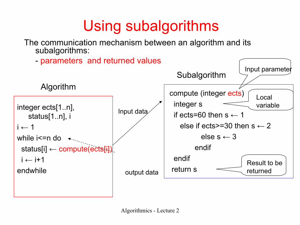
Using subalgorithmsThe communication mechanism between an algorithm and its
subalgorithms:- parameters and returned values
Algorithm
integer ects[1..n], status[1..n], i
i ← 1
while i<=n do
status[i] ← compute(ects[i])
i ← i+1
endwhile
compute (integer ects)
integer s
if ects=60 then s ← 1
else if ects>=30 then s ← 2
else s ← 3
endif
endif
return s
Subalgorithm
Input data
output data
Input parameter
Local variable
Result to be returned

Algorithmics - Lecture 2
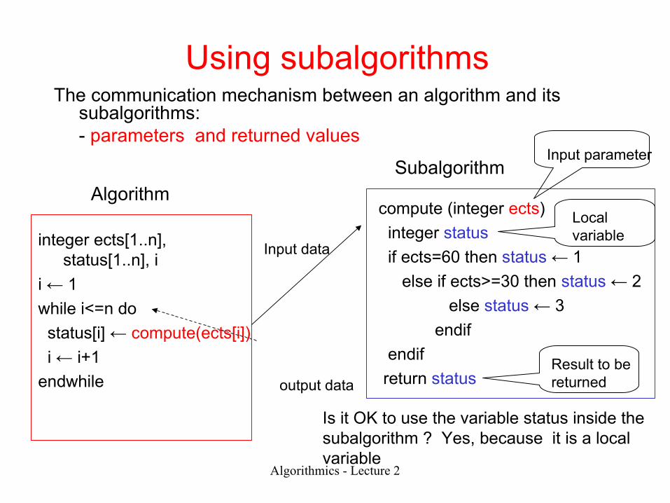
Using subalgorithmsThe communication mechanism between an algorithm and its
subalgorithms:- parameters and returned values
Algorithm
integer ects[1..n], status[1..n], i
i ← 1
while i<=n do
status[i] ← compute(ects[i])
i ← i+1
endwhile
compute (integer ects)
integer status
if ects=60 then status ← 1
else if ects>=30 then status ← 2
else status ← 3
endif
endif
return status
Subalgorithm
Input data
output data
Input parameter
Local variable
Result to be returned
Algorithmics - Lecture 2
Using subalgorithmsThe communication mechanism between an algorithm and its
subalgorithms:- parameters and returned values
Algorithm
integer ects[1..n], status[1..n], i
i ← 1
while i<=n do
status[i] ← compute(ects[i])
i ← i+1
endwhile
compute (integer ects)
integer status
if ects=60 then status ← 1
else if ects>=30 then status ← 2
else status ← 3
endif
endif
return status
Subalgorithm
Input data
output data
Input parameter
Local variable
Result to be returned
Is it OK to use the variable status inside thesubalgorithm ? Yes, because it is a localvariable

Algorithmics - Lecture 2
Using subalgorithms• Structure of a subalgorithm:
<subalgorithm name> (<formal parameters>)
< declaration of local variables >
< statements>
RETURN <results>
• Call of a subalgorithm:
<subalgorithm name> (<actual parameters>)

Back to Example 1
Pseudocode:
integer ects[1..n], status[1..n], i
i:=1
while i<=n do
status[i] ← compute(ects[i])
i:=i+1
endwhile
Another variant
integer ects[1..n], status[1..n], i
for i:=1,n do
status[i] ← compute(ects[i])
endfor
Subalgorithm (function) description:
compute (integer ects)
integer status
if ects=60 then status ← 1
else if ects>=30 then status ← 2
else status ← 3
endif
endif
return status

Example 1: Python implementation
Python program:
ects=[60,60,40,20,60]
status=[0]*5
n=5
i=0
while i<n:
status[i]=compute(ects[i])
i=i+1
print status
Using a for statement instead of while:
for i in range(5):
status[i]=compute(ects[i])
Python function (module):
def compute(ects):
if ects==60:
status=1
elif ects>=30:
status=2
else:
status=3
return status
Remark: indentation is very important in Python

Example 1: computation of the average
Compute the averaged mark
integer marks[1..n,1..m], status[1..n]
real avg[1..n]
…
for i ← 1,n do
if status[i]=1
avg[i] ← computeAvg(marks[i,1..m])
endif
endfor
Computation of an average
computeAvg(integer values[1..m])
real sum
integer i
sum ← 0
for i ← 1,m do
sum ← sum+values[i]
endfor
sum ← sum/m
return sum

Example 1: computation of the average
Compute the averaged mark (Python example)
marks=[[8,6,7],[10,10,10],[0,7,5],[6,0,0], [8,7,9]]
status=[1,1,2,3,1]
avg=[0]*5
for i in range(5):
if status[i]==1:
avg[i]=computeAvg(marks[i])
print avg
Computation of an average (Python example)
def computeAvg(marks):
m=len(marks)
sum=0
for i in range(m):
sum = sum+marks[i]
sum=sum/m
return sum
Algorithmics - Lecture 2 55
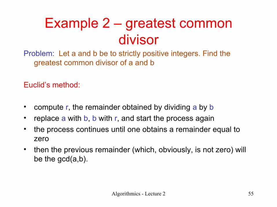
Example 2 – greatest common divisor
Problem: Let a and b be to strictly positive integers. Find the greatest common divisor of a and b
Euclid’s method:
• compute r, the remainder obtained by dividing a by b• replace a with b, b with r, and start the process again• the process continues until one obtains a remainder equal to
zero• then the previous remainder (which, obviously, is not zero) will
be the gcd(a,b).

Algorithmics - Lecture 2 56
Example 2 - greatest common divisor
How does this method work ?
1: a=bq1+r1, 0<=r1<b
2: b=r1q2+r2, 0<=r2<r1
3: r1=r2q3+r3, 0<=r3<r2
…
i: ri-2=ri-1qi+ri, 0<=ri<ri-1
…
n-1: rn-3=rn-2qn-1+rn-1, 0<=rn-1<rn-2
n : rn-2=rn-1qn, rn=0
Remarks:
• at each step the dividend is the previous divisor and the new divisor is the oldremainder• the sequence of remaindersis strictly decreasing, thus there exists a value n such
that rn=0 (the method is finite)• using these relations one can
prove that rn-1is indeed the gcd

Algorithmics - Lecture 2 57
Example 2 - greatest common divisor
The algorithm (WHILE variant):
integer a,b,dd,dr,r read a,b dd←a dr ← b r ← dd MOD dr while r<>0 do dd ← dr dr ← r r ← dd MOD dr endwhile write dr
The algorithm:
(REPEAT variant)
integer a,b,dd,dr,r
read a,b
dd ← a
dr ← b
repeat
r ← dd MOD dr
dd ← dr
dr ← r
until r=0
write dd

Algorithmics - Lecture 2 58
Example 2 – gcd of a set of values
• Problem: Find the greatest common divisor of a sequence of non-zero
natural numbers
• Example: gcd(12,8,10)=gcd(gcd(12,8),10)=gcd(4,10)=2
• Basic idea: compute the gcd of the first two elements, then compute the gcd
between the previous gcd and the third element and so on … natural to use a (sub)algorithm for computing the gcd of two
values

Algorithmics - Lecture 2 59
Example 2 – gcd of a set of values
• Structure of the algorithm:
gcd_sequence(INTEGER a[1..n])
INTEGER d,i
d ← gcd(a[1],a[2])
FOR i ← 3,n DO
d ← gcd(d,a[i])
ENDFOR
RETURN d
gcd(integer a,b) integer dd,dr,r dd←a dr ← b r ← dd MOD dr while r<>0 do dd ← dr dr ← r r ← dd MOD dr endwhile return dr

Algorithmics - Lecture 2 60
Example 3: The successor problem
Let us consider a natural number of 10 distinct digits. Compute the next number (in increasing order) in the sequence of all naturals consisting of 10 distinct digits.
Example: x= 6309487521
Next number consisting of different digits
6309512478

Algorithmics - Lecture 2 61
The successor problemStep 1. Find the largest index i having the property that x[i-1]<x[i]
Example: x= 6309487521 i=6 (the pair of digits 4 and 8)
Step 2. Find the smallest element x[k] in x[i..n] which is larger than x[i-1]
Example: x=6309487521 k=8 (the digit 5 has this property)
Step 3. Interchange x[k] with x[i-1]
Example: x=6309587421 (this is a value larger than the first one)
Step 4. Sort x[i..n] increasingly (in order to obtain the smaller number satisfying the requirements)
Example: x=6309512478 (it is enough to reverse the order of elements in x[i..n])
Algorithmics - Lecture 2 62
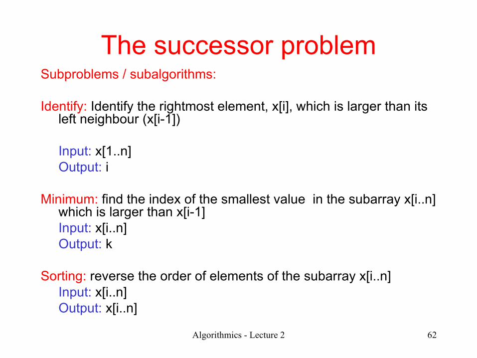
The successor problemSubproblems / subalgorithms:
Identify: Identify the rightmost element, x[i], which is larger than its left neighbour (x[i-1])
Input: x[1..n]Output: i
Minimum: find the index of the smallest value in the subarray x[i..n] which is larger than x[i-1] Input: x[i..n]Output: k
Sorting: reverse the order of elements of the subarray x[i..n]Input: x[i..n]Output: x[i..n]

Algorithmics - Lecture 2 63
The successor problemThe general structure of the algorithm:
Successor(integer x[1..n])integer i, k i←Identify(x[1..n])if i=1 then write “There is no successor !" else k ← Minimum(x[i..n]) x[i-1]↔x[k] x[i..n] ← Reverse(x[i..n]) write x[1..n]endif
Algorithmics - Lecture 2 64
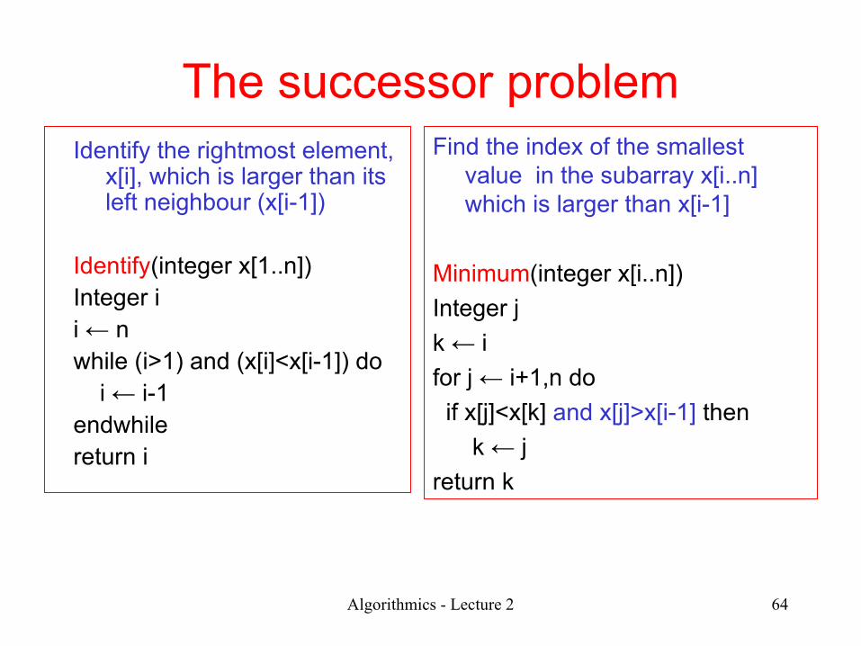
The successor problemIdentify the rightmost element,
x[i], which is larger than its left neighbour (x[i-1])
Identify(integer x[1..n])Integer ii ← nwhile (i>1) and (x[i]<x[i-1]) do i ← i-1endwhilereturn i
Find the index of the smallest value in the subarray x[i..n] which is larger than x[i-1]
Minimum(integer x[i..n])
Integer j
k ← i
for j ← i+1,n do
if x[j]<x[k] and x[j]>x[i-1] then
k ← j
return k

Algorithmics - Lecture 2 65
The successor problemReverse the order of elements of
a subarray of x
reverse (integer x[left..right]) integer i,j i ← left j ← right while i<j DO x[i]↔x[j] i ← i+1 j ← j-1 endwhile return x[left..right]

Algorithmics - Lecture 2 66
The successor problemPython implementation:def identify(x): n=len(x) i=n-1 while (i>0) and (x[i-1]>x[i]): i=i-1 return i
def minimum(x,i): n=len(x) k=i for j in range(i+1,n): if (x[j]<x[k]) and (x[j]>x[i-1]): k=j return k
def swap(a,b): aux=a a=b b=aux return a,b
def reverse(x,left,right): i=left j=right while i<j: x[i],x[j]=x[j],x[i] # other type of swap
i=i+1 j=j-1 return x

Algorithmics - Lecture 2 67
The successor problemPython implementation:
x=[6,3,0,9,4,8,7,5,2,1]print “Digits of the initial number :",xi=identify(x)print "i=",ik=minimum(x,i)print "k=",kx[i-1],x[k]=swap(x[i-1],x[k])print “Sequence after swap:",xx=reverse(x,i,len(x)-1)print “Sequence after reverse:",x

Algorithmics - Lecture 2 68
Summary
• The problems are usually decomposed in smaller subproblems solved by subalgorithms
• A subalgorithm is characterized through:– A name– Parameters (input data)– Returned values (output data)– Local variables (additional data)– Processing steps
• Call of a subalgorithm: – The parameters values are set to the input data– The statements of the subalgorithm are executed

Algorithmics - Lecture 2 69
Next lecture will be on …
• how to verify the correctness of an algorithm
• some formal methods in correctness verification


