
AMS526: Numerical Analysis I(Numerical Linear Algebra)
Lecture 7: Sensitivity of Linear Systems
Xiangmin Jiao
Stony Brook University
Xiangmin Jiao Numerical Analysis I 1 / 18

Outline
1 Condition Number of a Matrix
2 Perturbing Right-hand Side
3 Perturbing Coefficient Matrix
4 Putting All Together
Xiangmin Jiao Numerical Analysis I 2 / 18
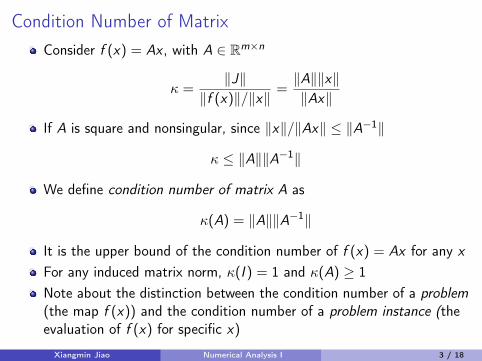
Condition Number of MatrixConsider f (x) = Ax , with A ∈ Rm×n
κ =‖J‖
‖f (x)‖/‖x‖=‖A‖‖x‖‖Ax‖
If A is square and nonsingular, since ‖x‖/‖Ax‖ ≤ ‖A−1‖
κ ≤ ‖A‖‖A−1‖
We define condition number of matrix A as
κ(A) = ‖A‖‖A−1‖
It is the upper bound of the condition number of f (x) = Ax for any xFor any induced matrix norm, κ(I ) = 1 and κ(A) ≥ 1Note about the distinction between the condition number of a problem(the map f (x)) and the condition number of a problem instance (theevaluation of f (x) for specific x)
Xiangmin Jiao Numerical Analysis I 3 / 18
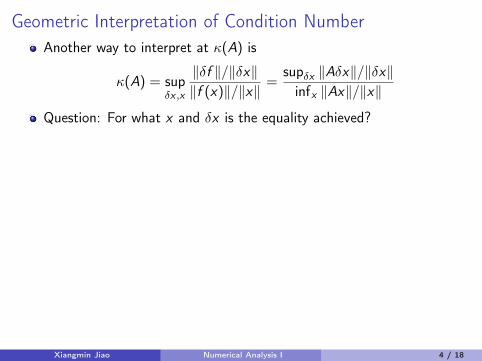
Geometric Interpretation of Condition NumberAnother way to interpret at κ(A) is
κ(A) = supδx ,x
‖δf ‖/‖δx‖‖f (x)‖/‖x‖
=supδx ‖Aδx‖/‖δx‖infx ‖Ax‖/‖x‖
Question: For what x and δx is the equality achieved?
Answer: When x is in direction of minimum magnification, and δx isin direction of maximum magnificationDefine maximum magnification of A as
maxmag(A) = max‖x‖=1
‖Ax‖
and minimum magnification of A as
minmag(A) = min‖x‖=1
‖Ax‖
Then condition number of matrix is κ(A) = maxmag(A)/minmag(A)For 2-norm, κ(A) = σ1/σn, the ratio of largest and smallest singularvalues (in later sections)
Xiangmin Jiao Numerical Analysis I 4 / 18
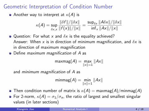
Geometric Interpretation of Condition NumberAnother way to interpret at κ(A) is
κ(A) = supδx ,x
‖δf ‖/‖δx‖‖f (x)‖/‖x‖
=supδx ‖Aδx‖/‖δx‖infx ‖Ax‖/‖x‖
Question: For what x and δx is the equality achieved?Answer: When x is in direction of minimum magnification, and δx isin direction of maximum magnificationDefine maximum magnification of A as
maxmag(A) = max‖x‖=1
‖Ax‖
and minimum magnification of A as
minmag(A) = min‖x‖=1
‖Ax‖
Then condition number of matrix is κ(A) = maxmag(A)/minmag(A)For 2-norm, κ(A) = σ1/σn, the ratio of largest and smallest singularvalues (in later sections)
Xiangmin Jiao Numerical Analysis I 4 / 18
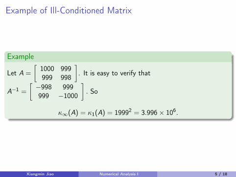
Example of Ill-Conditioned Matrix
Example
Let A =
[1000 999999 998
]. It is easy to verify that
A−1 =
[−998 999999 −1000
]. So
κ∞(A) = κ1(A) = 19992 = 3.996× 10⁶.
Xiangmin Jiao Numerical Analysis I 5 / 18
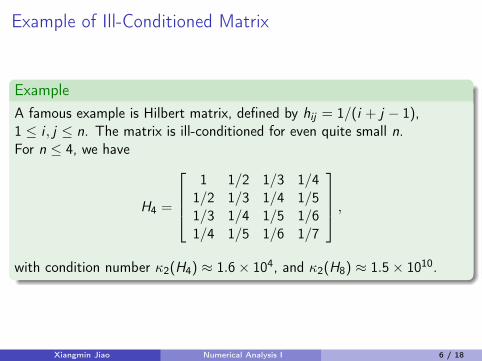
Example of Ill-Conditioned Matrix
ExampleA famous example is Hilbert matrix, defined by hij = 1/(i + j − 1),1 ≤ i , j ≤ n. The matrix is ill-conditioned for even quite small n.For n ≤ 4, we have
H4 =
1 1/2 1/3 1/4
1/2 1/3 1/4 1/51/3 1/4 1/5 1/61/4 1/5 1/6 1/7
,with condition number κ2(H4) ≈ 1.6× 10⁴, and κ2(H8) ≈ 1.5× 10¹⁰.
Xiangmin Jiao Numerical Analysis I 6 / 18

Outline
1 Condition Number of a Matrix
2 Perturbing Right-hand Side
3 Perturbing Coefficient Matrix
4 Putting All Together
Xiangmin Jiao Numerical Analysis I 7 / 18
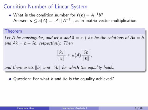
Condition Number of Linear SystemWhat is the condition number for f (b) = A−1b?
Answer: κ ≤ κ(A) ≡ ‖A‖‖A−1‖, as in matrix-vector multiplication
TheoremLet A be nonsingular, and let x and x = x + δx be the solutions of Ax = band Ax = b + δb, respectively. Then
‖δx‖‖x‖
≤ κ(A)‖δb‖‖b‖
,
and there exists ‖b‖ and ‖δb‖ for which the equality holds.
Question: For what b and δb is the equality achieved?Answer: When b is in direction of minimum magnification of A−1, andδb is in direction of maximum magnification of A−1.In 2-norm, when b is in direction of maximum magnification of AT ,and δb is in direction of minimum magnification of AT .
Xiangmin Jiao Numerical Analysis I 8 / 18
Condition Number of Linear SystemWhat is the condition number for f (b) = A−1b?Answer: κ ≤ κ(A) ≡ ‖A‖‖A−1‖, as in matrix-vector multiplication
TheoremLet A be nonsingular, and let x and x = x + δx be the solutions of Ax = band Ax = b + δb, respectively. Then
‖δx‖‖x‖
≤ κ(A)‖δb‖‖b‖
,
and there exists ‖b‖ and ‖δb‖ for which the equality holds.
Question: For what b and δb is the equality achieved?
Answer: When b is in direction of minimum magnification of A−1, andδb is in direction of maximum magnification of A−1.In 2-norm, when b is in direction of maximum magnification of AT ,and δb is in direction of minimum magnification of AT .
Xiangmin Jiao Numerical Analysis I 8 / 18
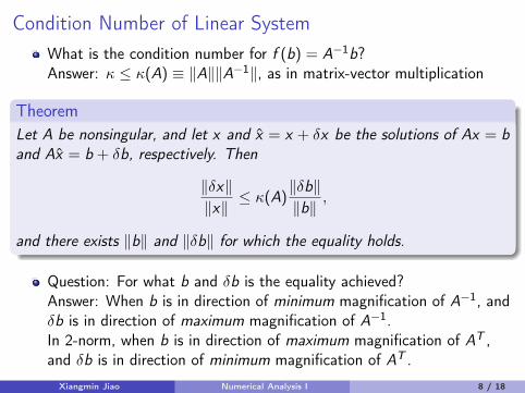
Condition Number of Linear SystemWhat is the condition number for f (b) = A−1b?Answer: κ ≤ κ(A) ≡ ‖A‖‖A−1‖, as in matrix-vector multiplication
TheoremLet A be nonsingular, and let x and x = x + δx be the solutions of Ax = band Ax = b + δb, respectively. Then
‖δx‖‖x‖
≤ κ(A)‖δb‖‖b‖
,
and there exists ‖b‖ and ‖δb‖ for which the equality holds.
Question: For what b and δb is the equality achieved?Answer: When b is in direction of minimum magnification of A−1, andδb is in direction of maximum magnification of A−1.In 2-norm, when b is in direction of maximum magnification of AT ,and δb is in direction of minimum magnification of AT .
Xiangmin Jiao Numerical Analysis I 8 / 18
Singular and Nearly Singular Linear System
Question: What is condition number of Ax if A is singular?
Answer: ∞.We say a matrix is nearly singular if its condition number is very largeIn other words, columns of A are nearly linearly dependentIf A is nearly singular, for matrix-vector multiplication, Ax , error islarge if x is nearly in null space of AIf A is nearly singular, for linear system Ax = b, error is large if b isNOT nearly in null space of AT
Therefore, ill-conditioning (near singularity) has a much bigger impacton solving linear system than matrix-vector multiplication!
Xiangmin Jiao Numerical Analysis I 9 / 18
Singular and Nearly Singular Linear System
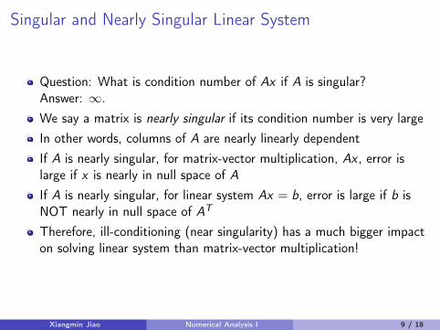
Question: What is condition number of Ax if A is singular?Answer: ∞.We say a matrix is nearly singular if its condition number is very largeIn other words, columns of A are nearly linearly dependentIf A is nearly singular, for matrix-vector multiplication, Ax , error islarge if x is nearly in null space of AIf A is nearly singular, for linear system Ax = b, error is large if b isNOT nearly in null space of AT
Therefore, ill-conditioning (near singularity) has a much bigger impacton solving linear system than matrix-vector multiplication!
Xiangmin Jiao Numerical Analysis I 9 / 18
Ill Conditioning Caused by Poor Scaling
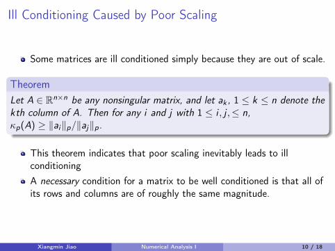
Some matrices are ill conditioned simply because they are out of scale.
TheoremLet A ∈ Rn×n be any nonsingular matrix, and let ak , 1 ≤ k ≤ n denote thekth column of A. Then for any i and j with 1 ≤ i , j ,≤ n,κp(A) ≥ ‖ai‖p/‖aj‖p.
This theorem indicates that poor scaling inevitably leads to illconditioningA necessary condition for a matrix to be well conditioned is that all ofits rows and columns are of roughly the same magnitude.
Xiangmin Jiao Numerical Analysis I 10 / 18

Estimating Condition Number
We would like to estimate κ1(A) = ‖A‖1‖A−1‖1 without computingA−1, but allow LU factorization of AFor any vector w ∈ Rn and ‖w‖1 = 1, we have lower bound
κ1(A) ≥ ‖A‖1‖A−1w‖1
If w has a significant component in direction near maximummagnification by A−1, then
κ1(A) ≈ ‖A‖1‖A−1w‖1
Note statement on p. 132 of textbook “Actually any w chosen atrandom is likely to have a significant component in the direction ofmaximum magnification by A−1” is unjustified for large n in 1-normGood estimators conduct systematic searches for w that approximatelymaximizes ‖A−1w‖1
Xiangmin Jiao Numerical Analysis I 11 / 18

Outline
1 Condition Number of a Matrix
2 Perturbing Right-hand Side
3 Perturbing Coefficient Matrix
4 Putting All Together
Xiangmin Jiao Numerical Analysis I 12 / 18
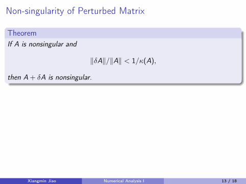
Non-singularity of Perturbed Matrix
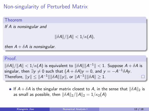
TheoremIf A is nonsingular and
‖δA‖/‖A‖ < 1/κ(A),
then A+ δA is nonsingular.
Proof.‖δA‖/‖A‖ < 1/κ(A) is equivalent to ‖δA‖‖A−1‖ < 1. Suppose A+ δA issingular, then ∃y 6= 0 such that (A+ δA)y = 0, and y = −A−1δAy .Therefore, ‖y‖ ≤ ‖A−1‖‖δA‖‖y‖, or ‖A−1‖‖δA‖ ≥ 1.
If A+ δA is the singular matrix closest to A, in the sense that ‖δA‖2 isas small as possible, then ‖δA‖2/‖A‖2 = 1/κ2(A)
Xiangmin Jiao Numerical Analysis I 13 / 18
Non-singularity of Perturbed Matrix
TheoremIf A is nonsingular and
‖δA‖/‖A‖ < 1/κ(A),
then A+ δA is nonsingular.
Proof.‖δA‖/‖A‖ < 1/κ(A) is equivalent to ‖δA‖‖A−1‖ < 1. Suppose A+ δA issingular, then ∃y 6= 0 such that (A+ δA)y = 0, and y = −A−1δAy .Therefore, ‖y‖ ≤ ‖A−1‖‖δA‖‖y‖, or ‖A−1‖‖δA‖ ≥ 1.
If A+ δA is the singular matrix closest to A, in the sense that ‖δA‖2 isas small as possible, then ‖δA‖2/‖A‖2 = 1/κ2(A)
Xiangmin Jiao Numerical Analysis I 13 / 18
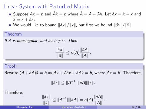
Linear System with Perturbed MatrixSuppose Ax = b and Ax = b where A = A+ δA. Let δx = x − x andx = x + δx .We would like to bound ‖δx‖/‖x‖, but first we bound ‖δx‖/‖x‖
TheoremIf A is nonsingular, and let b 6= 0. Then
‖δx‖‖x‖
≤ κ(A)‖δA‖‖A‖
.
Proof.Rewrite (A+ δA)x = b as Ax +Aδx + δAx = b, where Ax = b. Therefore,
‖δx‖ ≤ ‖A−1‖‖δA‖‖x‖.
Therefore,‖δx‖‖x‖
≤ ‖A−1‖‖δA‖ = κ(A)‖δA‖‖A‖
.
Xiangmin Jiao Numerical Analysis I 14 / 18
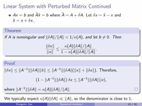
Linear System with Perturbed Matrix ContinuedAx = b and Ax = b where A = A+ δA. Let δx = x − x andx = x + δx .
TheoremIf A is nonsingular and ‖δA‖/‖A‖ < 1/κ(A), and let b 6= 0. Then
‖δx‖‖x‖
≤ κ(A)‖δA‖/‖A‖1− κ(A)‖δA‖/‖A‖
.
Proof.‖δx‖ ≤ ‖A−1‖‖δA‖‖x‖ ≤ ‖A−1‖‖δA‖(‖x‖+ ‖δx‖). Therefore,(
1− ‖A−1‖‖δA‖)δx ≤ ‖A−1‖‖δA‖‖x‖,
where ‖A−1‖‖δA‖ = κ(A)‖δA‖/‖A‖.
We typically expect κ(A)‖δA‖ � ‖A‖, so the denominator is close to 1.Xiangmin Jiao Numerical Analysis I 15 / 18

Outline
1 Condition Number of a Matrix
2 Perturbing Right-hand Side
3 Perturbing Coefficient Matrix
4 Putting All Together
Xiangmin Jiao Numerical Analysis I 16 / 18
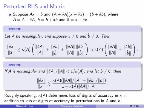
Perturbed RHS and MatrixSuppose Ax = b and (A+ δA)(x + δx) = (b + δb), whereA = A+ δA, b = b + δb and x = x + δx .
Theorem
Let A be nonsingular, and suppose x 6= 0 and b 6= 0. Then
‖δx‖‖x‖
≤ κ(A)
(‖δA‖‖A‖
+‖δb‖‖b‖
+‖δA‖‖A‖
‖δb‖‖b‖
)≈ κ(A)
(‖δA‖‖A‖
+‖δb‖‖b‖
).
TheoremIf A is nonsingular and ‖δA‖/‖A‖ < 1/κ(A), and let b 6= 0, then
‖δx‖‖x‖
.κ(A)(‖δA‖/‖A‖+ ‖δb‖/‖b‖)
1− κ(A)‖δA‖/‖A‖.
Roughly speaking, κ(A) determines loss of digits of accuracy in x inaddition to loss of digits of accuracy in perturbations in A and b
Xiangmin Jiao Numerical Analysis I 17 / 18
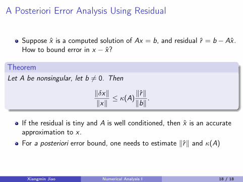
A Posteriori Error Analysis Using Residual
Suppose x is a computed solution of Ax = b, and residual r = b−Ax .How to bound error in x − x?
TheoremLet A be nonsingular, let b 6= 0. Then
‖δx‖‖x‖
≤ κ(A) ‖r‖‖b‖
.
If the residual is tiny and A is well conditioned, then x is an accurateapproximation to x .For a posteriori error bound, one needs to estimate ‖r‖ and κ(A)
Xiangmin Jiao Numerical Analysis I 18 / 18


