Download - An Introduction to Low Density Parity Check (LDPC) Codesmat.hjg.com.ar/tic/img/slideldpc.pdf · An Introduction to Low Density Parity Check (LDPC) Codes Jian Sun ... WCRL Seminar

WCRL Seminar Series LDPC Codes

An Introduction to Low Density

Parity Check (LDPC) Codes

Jian [email protected]

Wireless Communication Research Laboratory

Lane Dept. of Comp. Sci. and Elec. Engr.

West Virginia University

June 3, 2003 West Virginia University 1


Outline

1. History of LDPC codes

2. Properties of LDPC codes

3. Basics of LDPC codes

• Encoding of LDPC codes

• Iterative decoding of LDPC codes

• Simplified approximations of LDPC decoders

4. Applications of LDPC codes



Features of LDPC Codes

• Approaching Shannon capacity

– For example, 0.3 dB from Shannon limit

– Irregular LDPC code with code length 1 million. (Richardson:1999)

– An closer design from (Chung:2001), 0.0045 dB away from capapcity

• Good block error correcting performance

• Low error floor

– The minimum distance is proportional to code length

• Linear decoding complexity in time

• Suitable for parallel implementation



History of LDPC Codes

• Invented by Robert Gallager in his 1960 MIT Ph. D. dissertation. Long time being

ignored due to

1. Requirement of high complexity computation

2. Introduction of Reed-Solomon codes

3. The concatenated RS and convolutional codes were considered perfectly suitable

for error control coding.

• Rediscovered by MacKay(1999) and Richardson/Urbanke(1998).



Foundamentals of Linear Block Codes

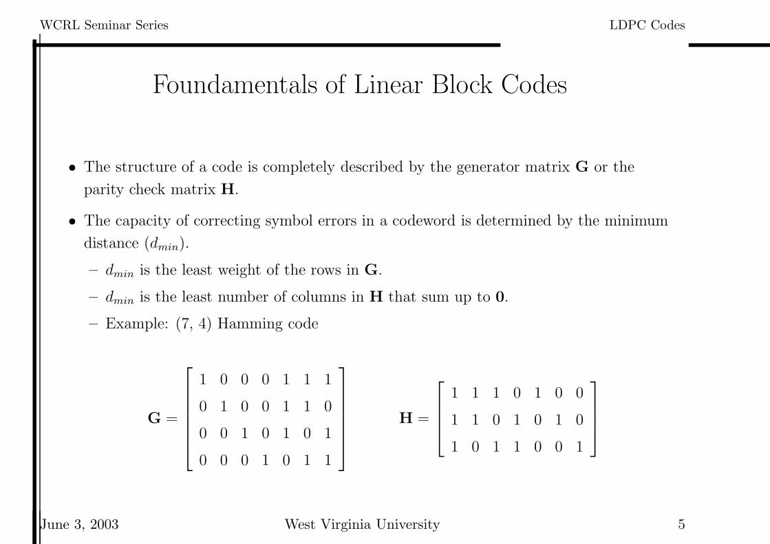
• The structure of a code is completely described by the generator matrix G or the

parity check matrix H.

• The capacity of correcting symbol errors in a codeword is determined by the minimum

distance (dmin).

– dmin is the least weight of the rows in G.

– dmin is the least number of columns in H that sum up to 0.

– Example: (7, 4) Hamming code

G =

1 0 0 0 1 1 1

0 1 0 0 1 1 0

0 0 1 0 1 0 1

0 0 0 1 0 1 1

H =

1 1 1 0 1 0 0

1 1 0 1 0 1 0

1 0 1 1 0 0 1



Properties of LDPC Codes

• H is sparse.

– Very few 1’s in each row and column.

– Expected large minimum distance.

• Regular LDPC codes

– H contains exactly Wc 1’s per column and exactly Wr = Wc(n/m) 1’s per row,

where Wc << m.

– The above definition implies that Wr << n.

– Wc ≥ 3 is necessary for good codes.

• If the number of 1’s per column or row is not constant, the code is an irregular LDPC

code.

– Usually irregular LDPC codes outperforms regular LDPC codes.



A Sample LDPC Code

H =

1 1 0 0

0 0 0 0

0 1 1 0

0 0 0 0

1 0 1 1

1 0 0 0

0 0 0 1

0 0 0 0

0 1 0 1

0 0 1 0...

· · ·

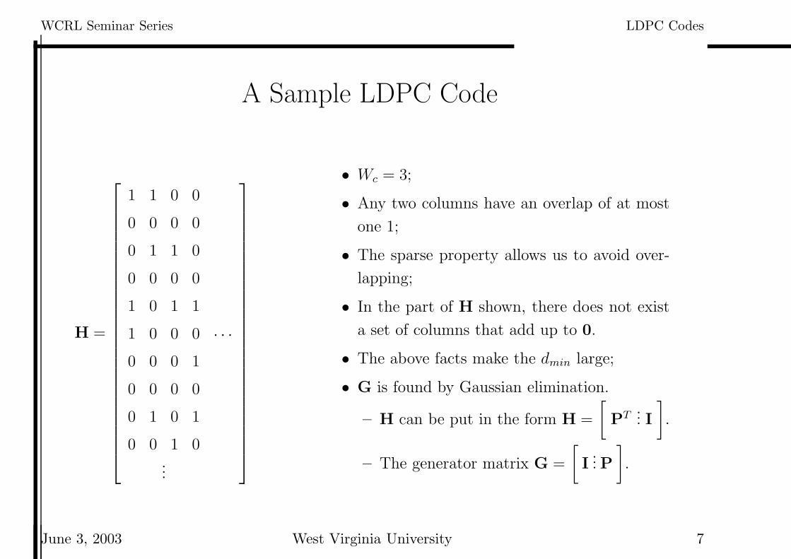
• Wc = 3;

• Any two columns have an overlap of at most

one 1;

• The sparse property allows us to avoid over-

lapping;

• In the part of H shown, there does not exist

a set of columns that add up to 0.

• The above facts make the dmin large;

• G is found by Gaussian elimination.

– H can be put in the form H =

[

PT ... I

]

.

– The generator matrix G =

[

I... P

]

.



Encoding of LDPC Codes

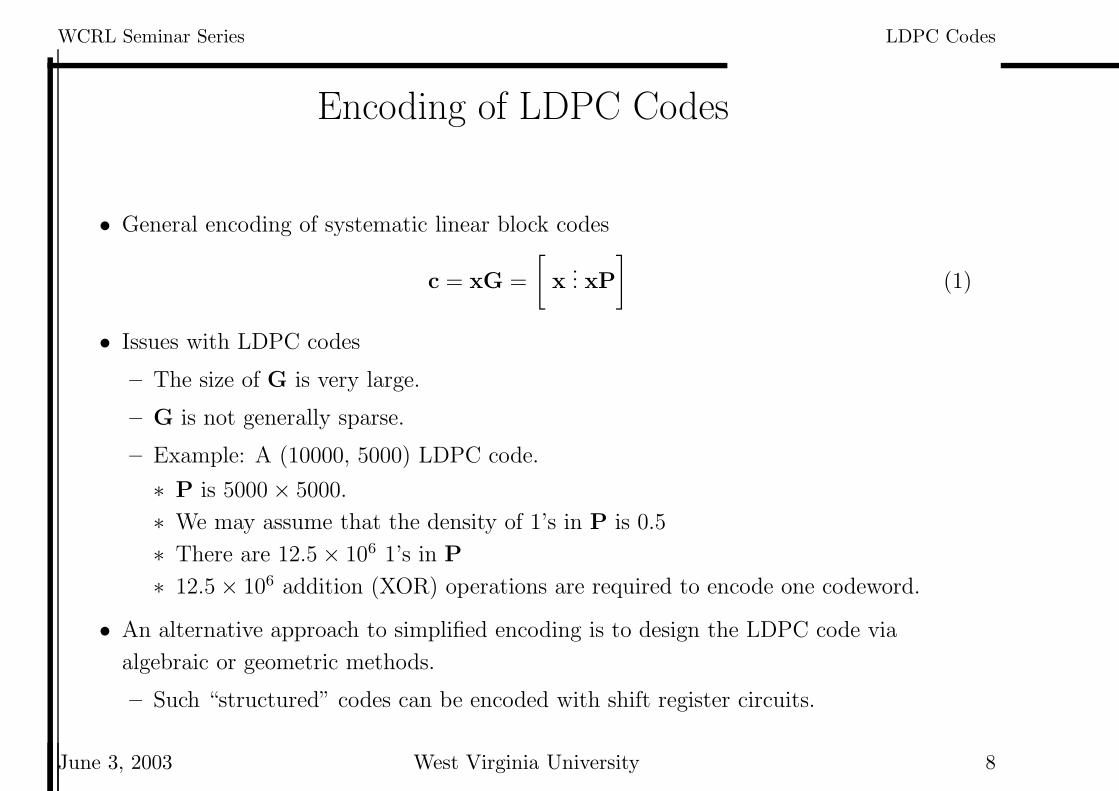
• General encoding of systematic linear block codes

c = xG =

[

x... xP

]

(1)

• Issues with LDPC codes

– The size of G is very large.

– G is not generally sparse.

– Example: A (10000, 5000) LDPC code.

∗ P is 5000 × 5000.

∗ We may assume that the density of 1’s in P is 0.5

∗ There are 12.5 × 106 1’s in P

∗ 12.5 × 106 addition (XOR) operations are required to encode one codeword.

• An alternative approach to simplified encoding is to design the LDPC code via

algebraic or geometric methods.

– Such “structured” codes can be encoded with shift register circuits.



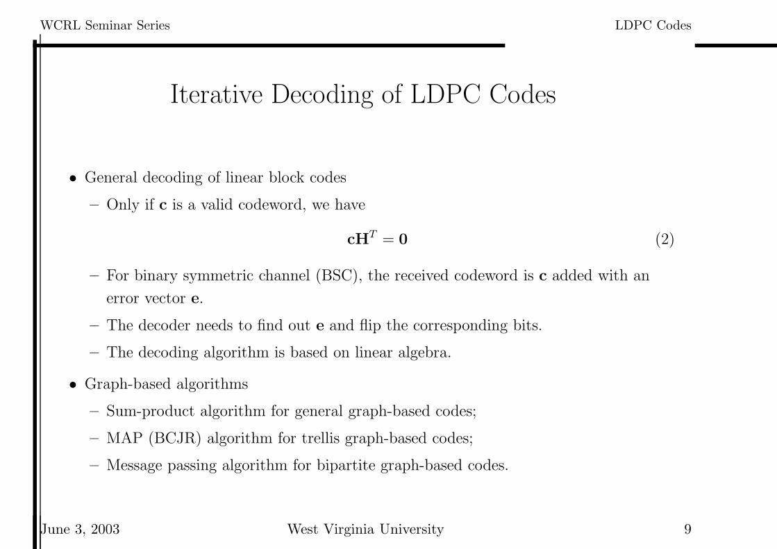
Iterative Decoding of LDPC Codes

• General decoding of linear block codes

– Only if c is a valid codeword, we have

cHT = 0 (2)

– For binary symmetric channel (BSC), the received codeword is c added with an

error vector e.

– The decoder needs to find out e and flip the corresponding bits.

– The decoding algorithm is based on linear algebra.

• Graph-based algorithms

– Sum-product algorithm for general graph-based codes;

– MAP (BCJR) algorithm for trellis graph-based codes;

– Message passing algorithm for bipartite graph-based codes.



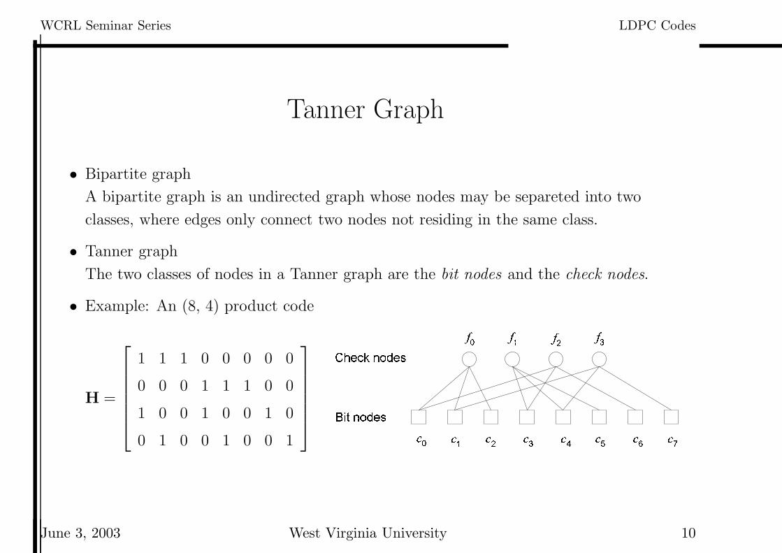
Tanner Graph

• Bipartite graph

A bipartite graph is an undirected graph whose nodes may be separeted into two

classes, where edges only connect two nodes not residing in the same class.

• Tanner graph

The two classes of nodes in a Tanner graph are the bit nodes and the check nodes.

• Example: An (8, 4) product code

H =

1 1 1 0 0 0 0 0

0 0 0 1 1 1 0 0

1 0 0 1 0 0 1 0

0 1 0 0 1 0 0 1

��

� � � � ��

�

�

� ��

� ��



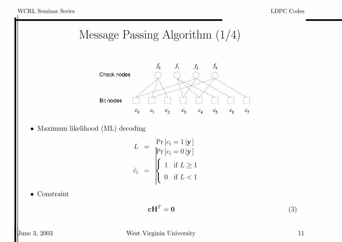
Message Passing Algorithm (1/4)

��

� !� � � ��

" #

$ #

" %" &" '

$ ($ )$ *$ +$ %$ &$ '

• Maximum likelihood (ML) decoding

L =Pr [ci = 1 |y ]

Pr [ci = 0 |y ]

ci =

1 if L ≥ 1

0 if L < 1

• Constraint

cHT = 0 (3)



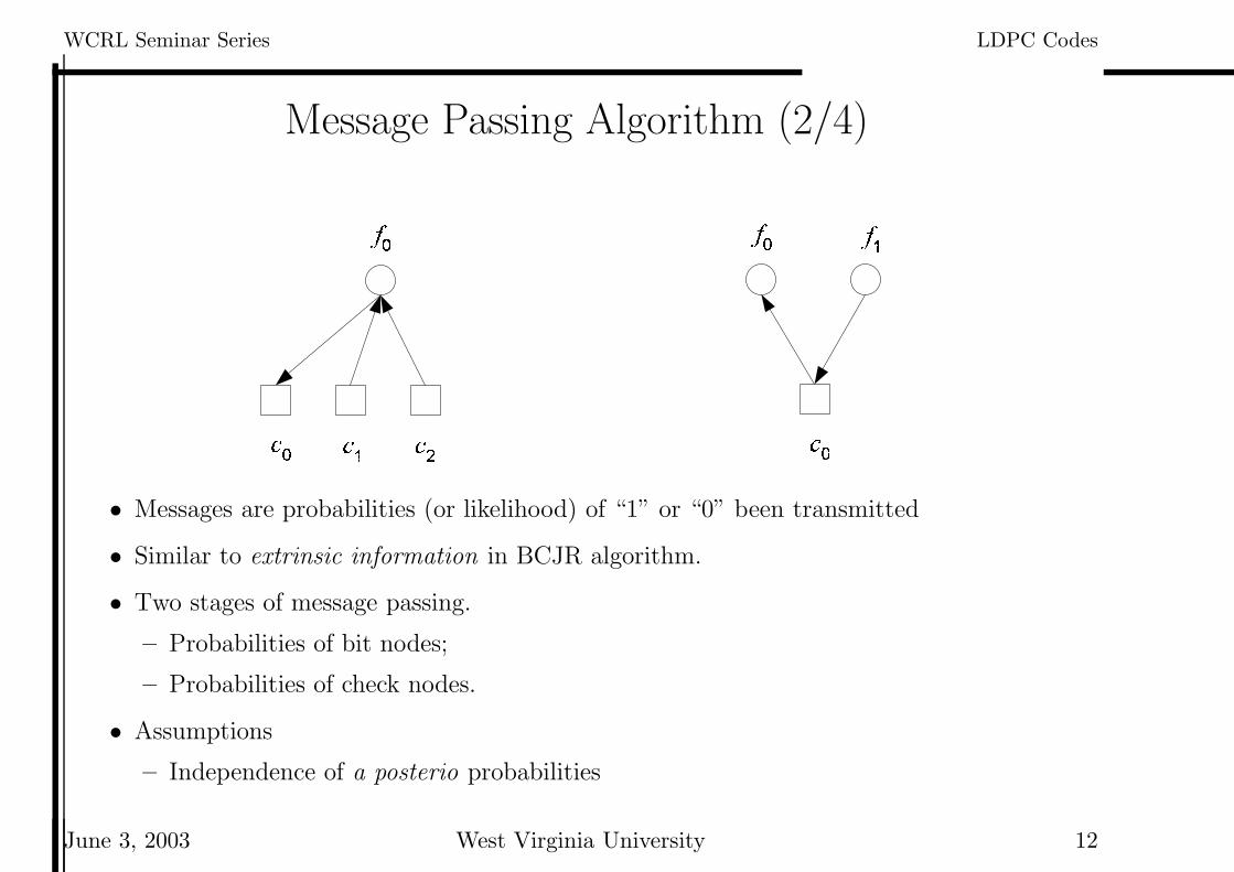
Message Passing Algorithm (2/4)

, -

. - . /. 0

1 2

3 2

1 4

• Messages are probabilities (or likelihood) of “1” or “0” been transmitted

• Similar to extrinsic information in BCJR algorithm.

• Two stages of message passing.

– Probabilities of bit nodes;

– Probabilities of check nodes.

• Assumptions

– Independence of a posterio probabilities



Message Passing Algorith (3/4)

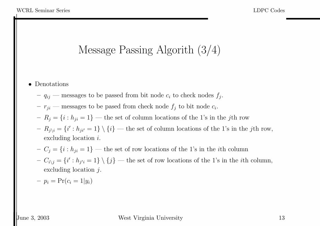
• Denotations

– qij — messages to be passed from bit node ci to check nodes fj .

– rji — messages to be pased from check node fj to bit node ci.

– Rj = {i : hji = 1} — the set of column locations of the 1’s in the jth row

– Rj\i = {i′ : hji′ = 1} \ {i} — the set of column locations of the 1’s in the jth row,

excluding location i.

– Cj = {i : hji = 1} — the set of row locations of the 1’s in the ith column

– Ci\j = {i′ : hj′i = 1} \ {j} — the set of row locations of the 1’s in the ith column,

excluding location j.

– pi = Pr(ci = 1|yi)



Message Passing Algorith (4/4)

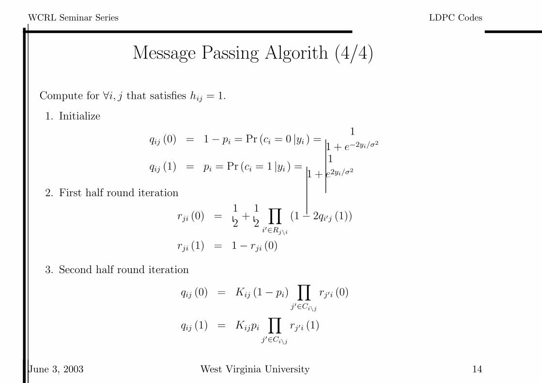
Compute for ∀i, j that satisfies hij = 1.

1. Initialize

qij (0) = 1 − pi = Pr (ci = 0 |yi ) =1

1 + e−2yi/σ2

qij (1) = pi = Pr (ci = 1 |yi ) =1

1 + e2yi/σ2

2. First half round iteration

rji (0) =1

2+

1

2

∏

i′∈Rj\i

(1 − 2qi′j (1))

rji (1) = 1 − rji (0)

3. Second half round iteration

qij (0) = Kij (1 − pi)∏

j′∈Ci\j

rj′i (0)

qij (1) = Kijpi

∏

j′∈Ci\j

rj′i (1)



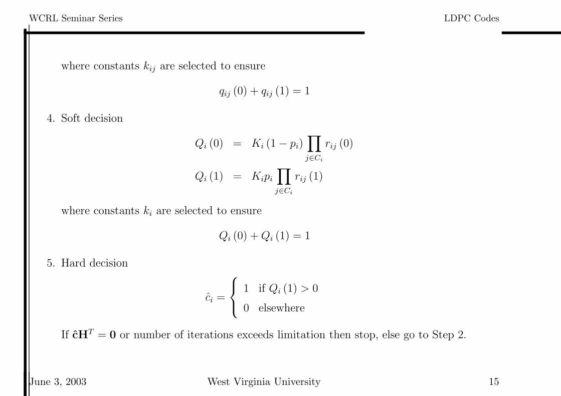
where constants kij are selected to ensure

qij (0) + qij (1) = 1

4. Soft decision

Qi (0) = Ki (1 − pi)∏

j∈Ci

rij (0)

Qi (1) = Kipi

∏

j∈Ci

rij (1)

where constants ki are selected to ensure

Qi (0) + Qi (1) = 1

5. Hard decision

ci =

1 if Qi (1) > 0

0 elsewhere

If cHT = 0 or number of iterations exceeds limitation then stop, else go to Step 2.



Log-Domain Algorithm (1/2)

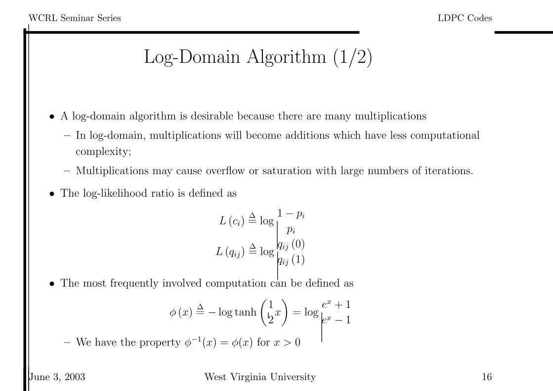
• A log-domain algorithm is desirable because there are many multiplications

– In log-domain, multiplications will become additions which have less computational

complexity;

– Multiplications may cause overflow or saturation with large numbers of iterations.

• The log-likelihood ratio is defined as

L (ci)∆= log

1 − pi

pi

L (qij)∆= log

qij (0)

qij (1)

• The most frequently involved computation can be defined as

φ (x)∆= − log tanh

(

1

2x

)

= logex + 1

ex − 1

– We have the property φ−1(x) = φ(x) for x > 0



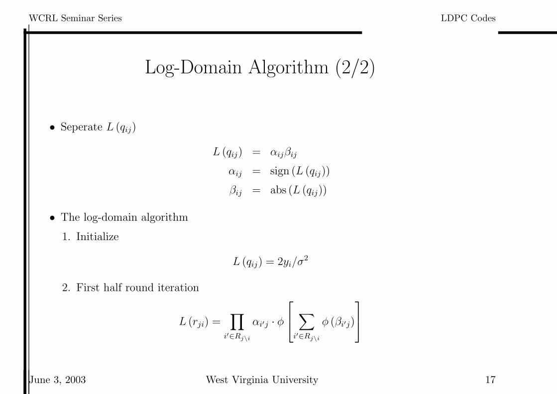
Log-Domain Algorithm (2/2)

• Seperate L (qij)

L (qij) = αijβij

αij = sign (L (qij))

βij = abs (L (qij))

• The log-domain algorithm

1. Initialize

L (qij) = 2yi/σ2

2. First half round iteration

L (rji) =∏

i′∈Rj\i

αi′j · φ

∑

i′∈Rj\i

φ (βi′j)



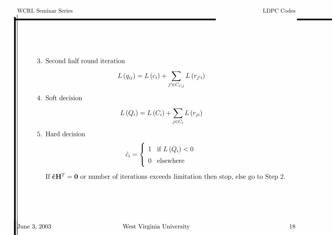
3. Second half round iteration

L (qij) = L (ci) +∑

j′∈Ci\j

L (rj′i)

4. Soft decision

L (Qi) = L (Ci) +∑

j∈Ci

L (rji)

5. Hard decision

ci =

1 if L (Qi) < 0

0 elsewhere

If cHT = 0 or number of iterations exceeds limitation then stop, else go to Step 2.



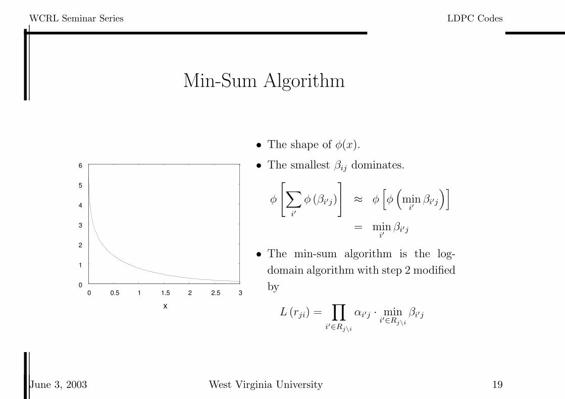
Min-Sum Algorithm

0 0.5 1 1.5 2 2.5 30

1

2

3

4

5

6

x

• The shape of φ(x).

• The smallest βij dominates.

φ

[

∑

i′

φ (βi′j)

]

≈ φ[

φ(

mini′

βi′j

)]

= mini′

βi′j

• The min-sum algorithm is the log-

domain algorithm with step 2 modified

by

L (rji) =∏

i′∈Rj\i

αi′j · mini′∈Rj\i

βi′j



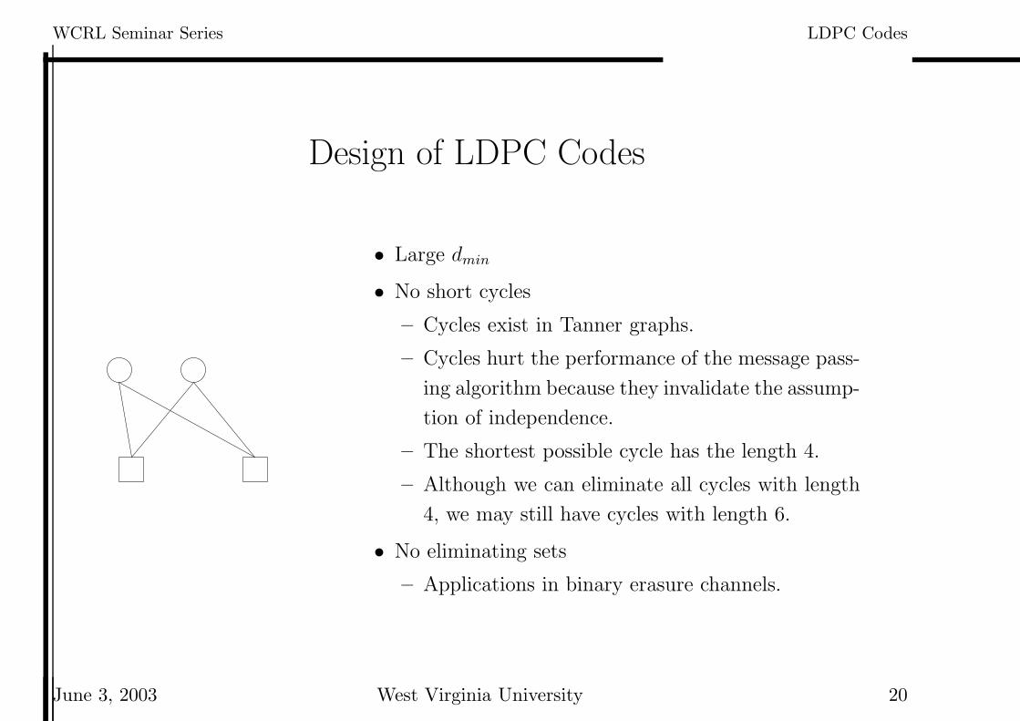
Design of LDPC Codes

• Large dmin

• No short cycles

– Cycles exist in Tanner graphs.

– Cycles hurt the performance of the message pass-

ing algorithm because they invalidate the assump-

tion of independence.

– The shortest possible cycle has the length 4.

– Although we can eliminate all cycles with length

4, we may still have cycles with length 6.

• No eliminating sets

– Applications in binary erasure channels.



Open Problems in LDPC Codes

• LDPC codes with near-capacity performance

– Very long codewords, many iterations, low signal-to-noise ratio.

• LDPC codes with relatively short codeword

– High coding rate r ≈ 1

– Short codewords enable easy encoding

• Combination with other technologies

– LDPC codes with OFDM systems

– LDPC codes with MIMO systems



References

[1] R. Gallager, “Low-density parity-check codes,” IRE Trans. Information Theory, pp. 21–28, January1962.

[2] D. MacKay, “Good error correcting codes based on very sparse matrices,” IEEE Trans. Information

Theory, pp. 399–431, March 1999.

[3] J. L. Fan, Constrained coding and soft iterative decoding for storage. PhD thesis, Stanford University,1999.

[4] T. richardson, M. Shokrollahi, and R. Urbanke, “Design of capacity-approaching irregular low-densityparity-check codes,” IEEE Trans. Inform. Theory, vol. 47, pp. 638–656, Feb. 2001.

[5] Y. Kou, S. Lin, and M. Fossorier, “Low-density parity-check codes based on finite geometries: arediscovery and new results,” IEEE Trans. Inform. Theory, vol. 47, pp. 2711–2736, Nov. 2001.
