Download - An Iterative Modal Identification Algorithm for Structural ...cheng/papers/An-Iterative...An Iterative Modal Identification Algorithm for Structural Health Monitoring Using Wireless

An Iterative Modal Identification Algorithmfor Structural Health Monitoring UsingWireless Sensor Networks

Siavash Dorvash,a) Shamim N. Pakzad,b) and Liang Chengc)

A novel modal identification approach for the use of a wireless sensornetwork (WSN) for structural health monitoring is presented, in which the com-putational task is distributed among remote nodes to reduce the communicationburden of the network and, as a result, optimize the time and energy consumptionof the monitoring system. Considering the need for having an agile system tocapture the earthquake response and also the limited energy resource inWSN, such algorithms for speeding the analysis time and preserving energyare essential. The algorithm of this study, called iterative modal identification(IMID), relies on an iterative estimation method that solves for unknown param-eters in the absence of complete information about the system. Applying IMID inWSN-based monitoring systems results in significant savings in time and energy.Validation through implementation of the algorithm on numerically simulatedand experimental data illustrates the superior performance of this approach.[DOI: 10.1193/1.4000133]

INTRODUCTION

Structural health monitoring (SHM) techniques have been the focus of much research inrecent years and have significantly improved by incorporating advancements in sensing andcommunication technology. In the new generation of SHM systems, attention is turned to thescalability of the sensing network (Liu et al. 2003, Swartz et al. 2005, Pakzad et al. 2008).The hardware components for these scalable networks can be achieved by utilizing wirelesssensor networks (WSNs). A WSN integrates a base station and remote sensors, with com-putational capability, communicating with each other through radio signals. Reduction in theinstrumentation cost and labor, together with the capability of on-board processing at sensingnodes, are critical enhancements, brought to SHM systems by using WSN. Over the past fewyears, researchers have developed and deployed different WSN platforms for SHM andshown the potential that exists in application of WSN in the health monitoring of infrastruc-ture (Tanner et al. 2003, Lynch et al. 2004a, Chung et al. 2004, Lynch et al. 2005, Pakzadet al. 2008, Whelan and Janoyan 2009, Pakzad 2010, Kim et al. 2010, Cho et al. 2010, Janget al. 2010). While WSN makes the deployment of SHM more convenient, a few challengeshave restricted its application in large-scale and long-term health monitoring of structuralsystems. Major challenges in application of WSN are the latency in the process due to

Earthquake Spectra, Volume 29, No. 2, pages 339–365, May 2013; © 2013, Earthquake Engineering Research Institute

a) Ph.D. candidate, Department of Civil and Environmental Engineering, Lehigh University, Bethlehem, PAb) Assistant Professor, Department of Civil and Environmental Engineering, Lehigh University, Bethlehem, PAc) Associate Professor, Department of Computer Science and Engineering, Lehigh University, Bethlehem, PA

339

the low data bandwidth and the difficulties in providing operational power of sensors forlong-term monitoring. Particularly in the event of an earthquake, WSNs need to be respon-sive in capturing and processing the data. Thus, new approaches are required to address thesechallenges and make the existingWSN technology suitable for a wide variety of applications.

In recent years, different approaches have been developed to address the power consump-tion issue. Energy harvesting (Grisso et al. 2005), wireless power transmission (Das et al.1998), and optimal power usage strategy are some examples. While these methods rely ontechnological developments, the optimal usage strategy offers an efficient and integral way ofpreserving energy just by applying smart local algorithms on wireless units. In addition, evenwith the use of energy harvesting or wireless power, it is still necessary to manage the powerconsumption, and therefore optimal usage strategies are crucial.

The basic idea in the optimal usage is utilizing the on-board computational capability ofwireless sensors, aiming to minimize the required time and energy for estimating the state ofthe structure from the measured data. In a majority of WSN deployments for SHM, the net-work architecture is designed such that all data is sent to a central station for further dataprocessing. In such a central data processing scheme, a long time and a large portion of thefinite power resource is spent on wireless communication for transmission of collected data.However, through the use of an optimal usage strategy, a system can be designed such that itincorporates on-board computation and preserves time and power by avoiding the commu-nication of the entire collected data.

Because the transmission of raw data is time-consuming and a wasteful use of energyresources, data compression (Lynch et al. 2003, Sadhu et al. 2012) and data conversionapproaches, such as the use of frequency responses (Caffrey et al. 2004), have been devel-oped to reduce the volume of communication. Research has also been focused on distributingdamage detection algorithms to make them suitable for implementation onWSN (Lynch et al.2004b, Gao et al. 2006, Hackmann et al. 2008). More recently, further progress has beenmade toward the concept of local data processing for modal identification such that justan informative and condensed format of data is communicated through the network. Oneexample of distributed modal identification approaches is the use of regularized autoregres-sive (AR) models (Pakzad et al. 2011). This approach proposes a restriction on AR param-eters of the multivariate AR models that eliminates the computation of correlation betweensignals measured at nodes that are far apart, thus reducing the volume of data passed throughthe network. This approach is shown to result in an 85% savings in communication load insome cases (Pakzad et al. 2011). Another example is coordinated computing strategy(Nagayama and Spencer 2007, Sim et al. 2009), which divides the network into a numberof subnetworks with cluster heads in a hierarchical topology. In this design, all the leaf nodesin each subnetwork receive the data from cluster heads and estimate and broadcast thecorrelation functions (under the assumption of ambient excitation) for implementation ofEigensystem realization algorithm (ERA). Further improvement of the approach is theuse of decentralized random decrement technique (Sim et al. 2010), in which instead of trans-mission of raw data from cluster head to leaf nodes, the trigger crossing information is sentfor estimation of correlation functions. Through examples it is shown that broadcasting thetrigger crossing information, instead of raw data, could reduce the communication burden by20%–30%. Although these approaches reduce the amount of communicated data, they are

340 S. DORVASH, S. N. PAKZAD, AND L. CHENG

dependent on the network topology and restricted by underlying identification algorithms.Additionally, more algorithm improvement is still required to remedy the latency and powerconsumption issue that exists in current WSN deployments.

This paper presents a novel approach for modal identification of structural systems, sui-table for addressing challenges in application of WSN in SHM. The proposed algorithm,called iterative modal identification (IMID), assigns a computational task of modal identi-fication to each remote node and limits the data communication to transmission of onlymodal analysis results. An iterative algorithm is developed such that each sensing nodein the network sufficiently influences the final estimated results. The necessary requirementfor the implementation of the proposed algorithm is an initial estimate of the structural modalproperties, which can be available for many structural systems. This paper presents the for-mulation of this method, and as a proof of concept, the algorithm is implemented on numeri-cally simulated shear structures and two experimental models.

The organization of the rest of this paper is as follows: The next section presents thesignificance of distributed modal identification algorithms in preserving time and energythrough a detailed discussion on energy consumption of different components of a sensingnode in a network. Then the theory and methodology of the proposed algorithm is presented.Afterward, the implementation of the algorithm is discussed and the validation of the algo-rithm through the use of numerically simulated and experimental models is presented.Another section evaluates the enhancement in efficiency of the modal identification bythe use of the proposed algorithm, and finally, the last section presents conclusions onthe performance of the proposed algorithm and its potential in different aspects of SHM.

SIGNIFICANCE OF THE DISTRIBUTED MODALIDENTIFICATION ALGORITHMS

Latency in the data collection and prohibitive power consumption, as major drawbacks inapplication of wireless sensor networks in structural health monitoring, need special consid-erations in the design of WSN architecture. In a long-term SHM scenario, the monitoringsystem is expected to be prepared for collecting data and also for processing the data andextracting important information about the state of the structure. Due to the limited band-width in wireless networks, transmitting large volumes of data can take a prohibitively longtime. In a large-scale deployment, tens of megabytes (MBs) of data need to be transferredthrough the network while the bandwidth is strictly limited. In one of the large-scale deploy-ments of WSN, Pakzad et al. (2008) reported an average bandwidth of 550 bytes per secondin multihop data transmission, which resulted in about nine hours for transferring 20 MB ofdata from 64 sensor nodes to the base station. Such a delay prevents the monitoring systemfrom prompt response, which is particularly required in the event of an earthquake.

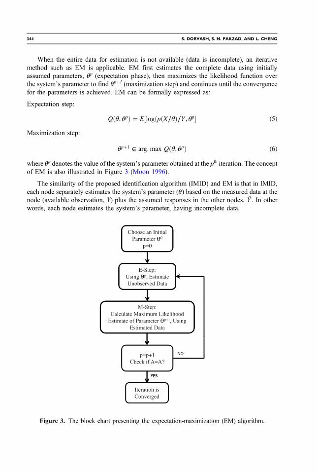
In addition to the latency caused by the data transmission, power consumption also limitsthe performance of WSNs in long-term monitoring. Different components of a wireless sen-sor unit for vibration monitoring (e.g., accelerometer, processor, and transceiver) consumedifferent amounts of energy when performing different tasks. Figure 1 shows a unit of awireless sensor platform with its different components: SHM-A sensor board (Rice andSpencer 2008) and Imote2 processing board (Crossbow 2007). Figure 2 presents a graphshowing the results of the power consumption measurement on this wireless sensor unit

AN ITERATIVE MODAL ID FOR SHMUSINGWIRELESS SENSOR NETWORKS 341

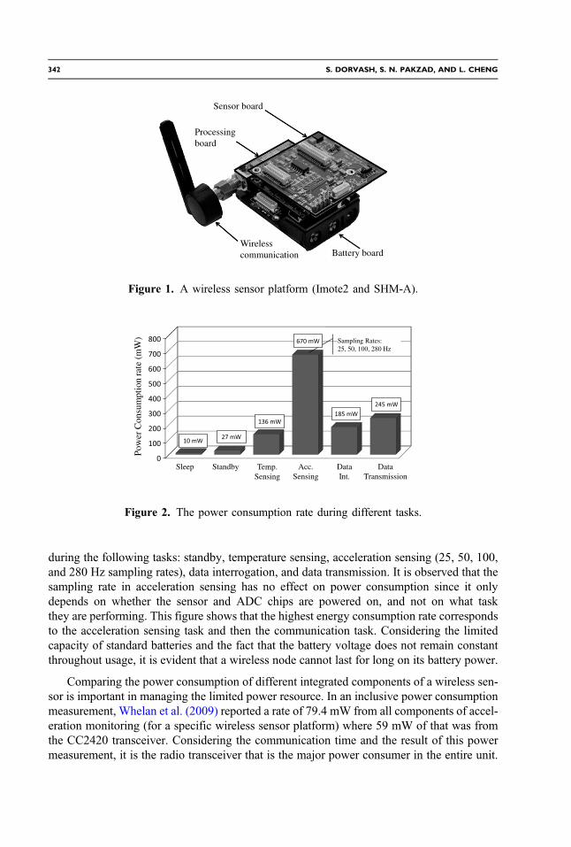
during the following tasks: standby, temperature sensing, acceleration sensing (25, 50, 100,and 280 Hz sampling rates), data interrogation, and data transmission. It is observed that thesampling rate in acceleration sensing has no effect on power consumption since it onlydepends on whether the sensor and ADC chips are powered on, and not on what taskthey are performing. This figure shows that the highest energy consumption rate correspondsto the acceleration sensing task and then the communication task. Considering the limitedcapacity of standard batteries and the fact that the battery voltage does not remain constantthroughout usage, it is evident that a wireless node cannot last for long on its battery power.

Comparing the power consumption of different integrated components of a wireless sen-sor is important in managing the limited power resource. In an inclusive power consumptionmeasurement, Whelan et al. (2009) reported a rate of 79.4 mW from all components of accel-eration monitoring (for a specific wireless sensor platform) where 59 mW of that was fromthe CC2420 transceiver. Considering the communication time and the result of this powermeasurement, it is the radio transceiver that is the major power consumer in the entire unit.

Sensor board

Processingboard

Wireless communication Battery board

Figure 1. A wireless sensor platform (Imote2 and SHM-A).

Figure 2. The power consumption rate during different tasks.


A distributed modal identification method incorporates the on-board processing capabil-ity to reduce the communication in the network. This approach is important because trans-mitting data over a wireless network not only takes a long time but also consumessignificantly more energy than performing a local computation. An approximation of therequired energy for performing a simple computation on one kB data and also for transmis-sion of the same data through the radio signal can be obtained as:

EQ-TARGET;temp:intralink-;e1;62;566Ecomputation ¼ ½Number of cycles f or computation ðALUÞ� � ½1∕Clock speed ðHzÞ�� ½Power consumption rate ðmWÞ� (1)

EQ-TARGET;temp:intralink-;e2;62;507Etrsmissionn ¼ ½1∕transmission rate ðKbpsÞ� � ½Power consumption rate ðmWÞ� (2)

where transmission rate, power consumption rate, and clock speed are specifications of thetransceiver and the processor. The number of required cycles for computation depends on thealgorithm that is used in the specific type of processor. ALU refers to arithmetic logic unit,which is a fundamental building block of a computer’s CPU.

Considering the specifications of the CC2420 transceiver (Chipcon AS SmartRF 2004)and an Intel PXA27x processor, which are integrated into the Imote2 platform (Crossbow2007), the estimated consumed energy for transmission of 1 kB of data is 0.24 mW/sec,whereas the estimated required energy for a simple computation on 1 kB of data is 2.25 �10−5 mW/sec. This result shows the noticeable higher power consumption of the transmissiontask and highlights the importance of developing and incorporating distributed modal identi-fication algorithms to reduce the communication load and to preserve the limited energy.

ITERATIVE MODAL IDENTIFICATION: THEORY AND METHODOLOGY

A basic requirement for most of the existing modal identification algorithms is access tothe entire measured data for computation of the full cross-correlation matrix. This restrictionrequires the sensor network to transmit all the collected data from each sensor to a basestation. The proposed algorithm, called IMID, estimates the modal parameters of the systemwithout requiring simultaneous access to the entire data.

IMID relies on a class of estimation algorithm called expectation-maximization (EM).EM estimates an unknown parameter (u) given the measurement data (Y ) in the presenceof some hidden variables (Y ) (Dempster 1977). This algorithm is in fact a generalizedform of maximum-likelihood estimation, which is applicable when the data is incomplete.Considering the log-likelihood function of unknown parameters u as:

EQ-TARGET;temp:intralink-;e3;62;184LðθÞ ¼ log½pðY∕θÞ� (3)

the estimation of unknowns (u) is given by maximizing the function, L(u), over u:

EQ-TARGET;temp:intralink-;e4;62;138θ ¼ Arg:max½LðθÞ� (4)

where Y is the available data (complete measured data).


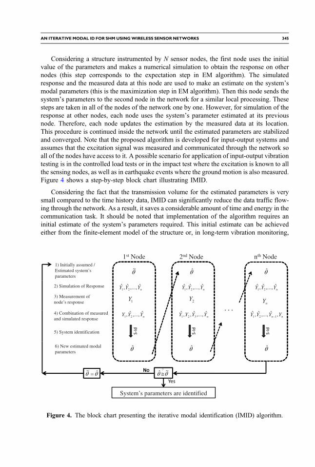
When the entire data for estimation is not available (data is incomplete), an iterativemethod such as EM is applicable. EM first estimates the complete data using initiallyassumed parameters, up (expectation phase), then maximizes the likelihood function overthe system’s parameter to find upþ1 (maximization step) and continues until the convergencefor the parameters is achieved. EM can be formally expressed as:

Expectation step:

EQ-TARGET;temp:intralink-;e5;41;560Qðθ; θpÞ ¼ E½logðpðX∕θÞ∕Y ; θp� (5)

Maximization step:

EQ-TARGET;temp:intralink-;e6;41;519θpþ1 ∈ arg:max Qðθ; θpÞ (6)

where up denotes the value of the system’s parameter obtained at the pth iteration. The conceptof EM is also illustrated in Figure 3 (Moon 1996).

The similarity of the proposed identification algorithm (IMID) and EM is that in IMID,each node separately estimates the system’s parameter (u) based on the measured data at thenode (available observation, Y) plus the assumed responses in the other nodes, Y . In otherwords, each node estimates the system’s parameter, having incomplete data.

Choose an Initial Parameter 0

p=0

E-Step:Using p, Estimate Unobserved Data

M-Step:Calculate Maximum Likelihood

Estimate of Parameter p+1, Using Estimated Data

p=p+1Check if A=A?

Iteration is Converged

Figure 3. The block chart presenting the expectation-maximization (EM) algorithm.


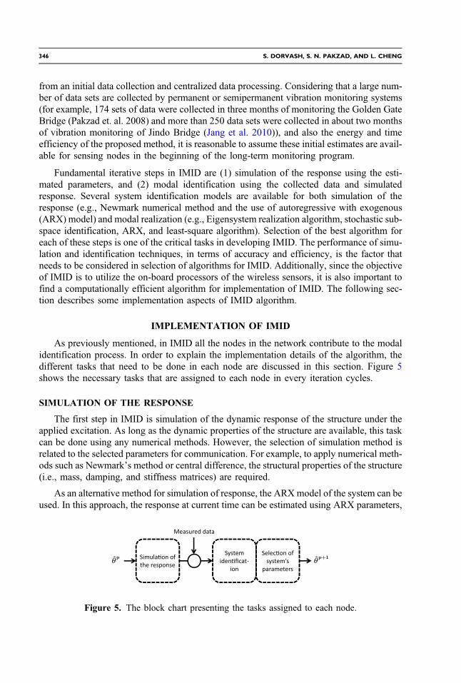
Considering a structure instrumented by N sensor nodes, the first node uses the initialvalue of the parameters and makes a numerical simulation to obtain the response on othernodes (this step corresponds to the expectation step in EM algorithm). The simulatedresponse and the measured data at this node are used to make an estimate on the system’smodal parameters (this is the maximization step in EM algorithm). Then this node sends thesystem’s parameters to the second node in the network for a similar local processing. Thesesteps are taken in all of the nodes of the network one by one. However, for simulation of theresponse at other nodes, each node uses the system’s parameter estimated at its previousnode. Therefore, each node updates the estimation by the measured data at its location.This procedure is continued inside the network until the estimated parameters are stabilizedand converged. Note that the proposed algorithm is developed for input-output systems andassumes that the excitation signal was measured and communicated through the network soall of the nodes have access to it. A possible scenario for application of input-output vibrationtesting is in the controlled load tests or in the impact test where the excitation is known to allthe sensing nodes, as well as in earthquake events where the ground motion is also measured.Figure 4 shows a step-by-step block chart illustrating IMID.

Considering the fact that the transmission volume for the estimated parameters is verysmall compared to the time history data, IMID can significantly reduce the data traffic flow-ing through the network. As a result, it saves a considerable amount of time and energy in thecommunication task. It should be noted that implementation of the algorithm requires aninitial estimate of the system’s parameters required. This initial estimate can be achievedeither from the finite-element model of the structure or, in long-term vibration monitoring,

1) Initially assumed / Estimated system’sparameters

~

1st Node

ˆ

2nd Node

ˆ

nth Node

2) Simulation of Response

3) Measurement of node’s response

nYYY ˆ,...,ˆ,ˆ21

1Y

nYYY ˆ,...,ˆ,ˆ21

2Y

nYYY ˆ,...,ˆ,ˆ21

nY

4) Combination of measured and simulated response

nYYY ˆ,...,ˆ, 21

5) System identification

nYYYY ˆ,...,ˆ,,ˆ321 nn YYYY ,ˆ,...,ˆ,ˆ

121

ˆ6) New estimated modal parameters

~ˆ?

ˆ~

ˆ ˆ

System’s parameters are identified

Figure 4. The block chart presenting the iterative modal identification (IMID) algorithm.


from an initial data collection and centralized data processing. Considering that a large num-ber of data sets are collected by permanent or semipermanent vibration monitoring systems(for example, 174 sets of data were collected in three months of monitoring the Golden GateBridge (Pakzad et. al. 2008) and more than 250 data sets were collected in about two monthsof vibration monitoring of Jindo Bridge (Jang et al. 2010)), and also the energy and timeefficiency of the proposed method, it is reasonable to assume these initial estimates are avail-able for sensing nodes in the beginning of the long-term monitoring program.

Fundamental iterative steps in IMID are (1) simulation of the response using the esti-mated parameters, and (2) modal identification using the collected data and simulatedresponse. Several system identification models are available for both simulation of theresponse (e.g., Newmark numerical method and the use of autoregressive with exogenous(ARX) model) and modal realization (e.g., Eigensystem realization algorithm, stochastic sub-space identification, ARX, and least-square algorithm). Selection of the best algorithm foreach of these steps is one of the critical tasks in developing IMID. The performance of simu-lation and identification techniques, in terms of accuracy and efficiency, is the factor thatneeds to be considered in selection of algorithms for IMID. Additionally, since the objectiveof IMID is to utilize the on-board processors of the wireless sensors, it is also important tofind a computationally efficient algorithm for implementation of IMID. The following sec-tion describes some implementation aspects of IMID algorithm.

IMPLEMENTATION OF IMID

As previously mentioned, in IMID all the nodes in the network contribute to the modalidentification process. In order to explain the implementation details of the algorithm, thedifferent tasks that need to be done in each node are discussed in this section. Figure 5shows the necessary tasks that are assigned to each node in every iteration cycles.

SIMULATION OF THE RESPONSE

The first step in IMID is simulation of the dynamic response of the structure under theapplied excitation. As long as the dynamic properties of the structure are available, this taskcan be done using any numerical methods. However, the selection of simulation method isrelated to the selected parameters for communication. For example, to apply numerical meth-ods such as Newmark’s method or central difference, the structural properties of the structure(i.e., mass, damping, and stiffness matrices) are required.

As an alternative method for simulation of response, the ARXmodel of the system can beused. In this approach, the response at current time can be estimated using ARX parameters,

Figure 5. The block chart presenting the tasks assigned to each node.


past response, and current and past inputs of the system. Utilizing ARX for simulation of theresponse requires ARX parameters to be transferred in the network.

MODAL IDENTIFICATION

After the dynamic response of the system is simulated at a remote node, the measuredresponse is replaced with the corresponding simulated response at that point and, togetherwith the simulated responses for other nodes, is fed into modal identification algorithm.

Consider the state-space representation of the dynamic system:

EQ-TARGET;temp:intralink-;e7;62;532xðnþ 1Þ ¼ AdxðnÞ þ BduðnÞ; (7)

EQ-TARGET;temp:intralink-;e8;62;492yðnÞ ¼ CxðnÞ þ DuðnÞ (8)

where x(n) is the state vector, y(n) is the observation vector, and u(n) is the input vector attime step n; Ad is the state and Bd is input matrices in discrete format, C is the observationmatrix and D is the transmission matrix. Eigenvalue decomposition of the state matrix (Ad)results in the matrices of eigenvalues (λi’s) and eigenvectors (ψ i’s) from which the naturalfrequencies, damping ratios, and mode shapes of the system can be obtained using the fol-lowing relationships:

EQ-TARGET;temp:intralink-;e9;62;389λci ; λ�ci ¼ �ζiωi � jωi

ffiffiffiffiffiffiffiffiffiffiffiffiffi1� ζ2i

q; (9)

EQ-TARGET;temp:intralink-;e10;62;342ϕi ¼ Cψ i; (10)

where ωi and ζi are natural frequencies and damping ratios, respectively, and λc is the eigen-value of the continuous state matrix, which can be obtained from this equation:

EQ-TARGET;temp:intralink-;e11;62;287λci ¼lnðλiÞΔt

(11)

where Δt is the sampling time. The goal in the identification step is to estimate the system(here, state-space matrices), which will result in accurate modal parameters.

SELECTION AND ASSESSMENT OF THE SYSTEM’S PARAMETERS FORTRANSMISSION

Estimation of the system’s parameters in IMID is not only the final objective but a stepthat is taken at each node in every iteration cycle. In fact, estimated parameters at each nodeare transmitted through the network to be updated node by node. Additionally, these param-eters are checked for convergence at each cycle. Therefore, it is important to select the mostinformative parameters representing the system. Several alternatives for the system’s param-eters are ARX parameters, state-space matrices, and modal properties of the structure.


The ARX parameters and state-space matrices can be the direct result of system identi-fication step and no further assessment is needed before transmission of the parameters. How-ever, extraction of structural properties (mass, damping, and stiffness matrices) from theresult of the system identification step needs some considerations. It should be noted thatthe advantage of selecting these properties, compared to other alternatives, is their compacttransmission volume.

Considering that the eigenvalues and eigenvectors of the system are estimated throughthe identification of the system’s matrices, from the second order equation of motion, theeigenvalue equation can be written as:

EQ-TARGET;temp:intralink-;e12;41;524ðλ2nmþ λncþ kÞψn ¼ 0 (12)

where λn and ψn are the nth complex eigenvalue and eigenvector of the dynamic system. Pre-

multiplying this equation by m−1, it can be rewritten as:

EQ-TARGET;temp:intralink-;e13;41;456½m�1k m�1c ��

ψn

λnψn

�¼ �λ2nψn (13)

which holds for each eigenvalue and eigenvector. Expanding the equation to include all nmodes of the system, it becomes:

EQ-TARGET;temp:intralink-;e14;41;376½m�1k m�1c ��

ψ1 ψ2 ... ψn

λ1ψ1 λ2ψ2 ... λnψn

�¼ �½ λ21ψ1 λ22ψ2 ... λ2nψn � (14)

or

EQ-TARGET;temp:intralink-;e15;41;311½m�1k m�1c � ¼ �½ λ21ψ1 λ22ψ2 ... λ2nψn ��

ψ1 ψ2 ... ψn

λ1ψ1 λ2ψ2 ... λnψn

��(15)

where * denotes the pseudo-inverse of a matrix. From this equation, ½m�1k� and ½m�1c� can beeasily extracted with the minimum least-square error. Having an estimate on the mass of thesystem, stiffness and damping can be obtained.

The remaining issue is determination of eigenvalues and eigenvectors associated with thephysical system from those generated by noise. During the system identification process, it iscommon to identify some modes that are not from the underlying physical system but are dueto the noise in the data and overparameterization of the problem (computational and spuriousmodes). Constructing a stability diagram (Peeters and Roeck 2001) is an approach thataddresses this difficulty based on the fact that structural modes stabilize through the processof increasing the model order whereas the spurious modes will not converge. Another avail-able approach is determination of confidence interval for modes through the consistent modeindicator (CMI) (Pappa et al. 1997). In implementation of IMID, having an initial estimate ofthe system is also an advantage that can assist with determination of structural modes from allidentified modes.


VALIDATION THROUGH NUMERICAL SIMULATION

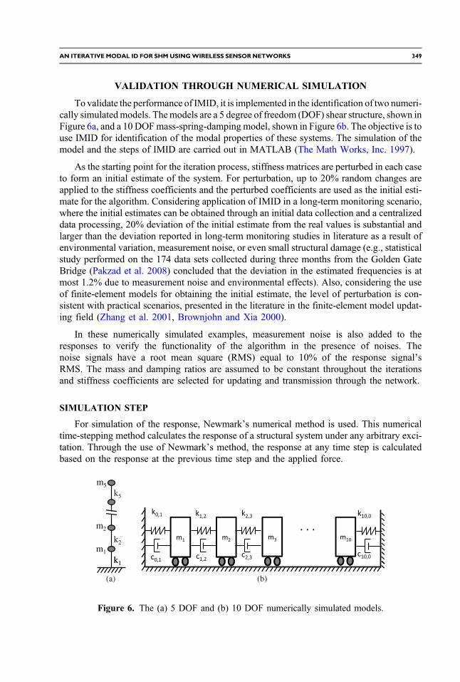
To validate the performance of IMID, it is implemented in the identification of two numeri-cally simulatedmodels. Themodels are a 5 degree of freedom (DOF) shear structure, shown inFigure 6a, and a 10 DOFmass-spring-damping model, shown in Figure 6b. The objective is touse IMID for identification of the modal properties of these systems. The simulation of themodel and the steps of IMID are carried out in MATLAB (The Math Works, Inc. 1997).

As the starting point for the iteration process, stiffness matrices are perturbed in each caseto form an initial estimate of the system. For perturbation, up to 20% random changes areapplied to the stiffness coefficients and the perturbed coefficients are used as the initial esti-mate for the algorithm. Considering application of IMID in a long-term monitoring scenario,where the initial estimates can be obtained through an initial data collection and a centralizeddata processing, 20% deviation of the initial estimate from the real values is substantial andlarger than the deviation reported in long-term monitoring studies in literature as a result ofenvironmental variation, measurement noise, or even small structural damage (e.g., statisticalstudy performed on the 174 data sets collected during three months from the Golden GateBridge (Pakzad et al. 2008) concluded that the deviation in the estimated frequencies is atmost 1.2% due to measurement noise and environmental effects). Also, considering the useof finite-element models for obtaining the initial estimate, the level of perturbation is con-sistent with practical scenarios, presented in the literature in the finite-element model updat-ing field (Zhang et al. 2001, Brownjohn and Xia 2000).

In these numerically simulated examples, measurement noise is also added to theresponses to verify the functionality of the algorithm in the presence of noises. Thenoise signals have a root mean square (RMS) equal to 10% of the response signal’sRMS. The mass and damping ratios are assumed to be constant throughout the iterationsand stiffness coefficients are selected for updating and transmission through the network.

SIMULATION STEP

For simulation of the response, Newmark’s numerical method is used. This numericaltime-stepping method calculates the response of a structural system under any arbitrary exci-tation. Through the use of Newmark’s method, the response at any time step is calculatedbased on the response at the previous time step and the applied force.

k5

m5

(a) (b)

k1

k2

m2

m1

k1

Figure 6. The (a) 5 DOF and (b) 10 DOF numerically simulated models.


IDENTIFICATION STEP

In order to estimate the system’s parameters, an ARX algorithm (Pandit 1991, Roecket al. 1995) is used. The ARX model can be written as:

EQ-TARGET;temp:intralink-;e16;41;598

Xpi¼0

αiyðn� iÞ ¼Xqi¼1

βixðn� iÞ þ eðnÞ (16)

where y ¼ ½y1ðnÞ y2ðnÞ ... ymðnÞ� and xðnÞ ¼ ½x1ðnÞ x2ðnÞ ... xrðnÞ� are matrices includingoutput and input vectors respectively, αi’s and βi’s are ARX coefficients, e(n) represents thenoise and measurement error, and p and q are orders of the autoregressive and exogenousparts of the ARX model that are assumed to be equal.

Having the AR parameters of the system, the state matrix can be expressed in the con-troller form as:

EQ-TARGET;temp:intralink-;e17;41;459A ¼

26666664

0 I : : 0 0

0 0 : : 0 0

: : : : : :: : : : : :0 0 : : 0 I

�αp �αp�1 : : : �α1

37777775

(17)

and also the observation matrix can be formed as:

EQ-TARGET;temp:intralink-;e18;41;344C ¼ ½ I 0 : : 0 0 � (18)

where [I] and [0] are identity and zero matrices with appropriate dimensions, respectively.From the state and observation matrices, modal properties of the system can be obtainedusing Equations 9–11.

RESULTS OF THE IMPLEMENTATION

To check the convergence of the results, the stiffness coefficients of the structure,identified frequencies, and mode shapes are assessed after each iteration cycle. The criterionfor convergence of modal properties is defined by a predetermined threshold for the estimatedparameters of the system at the end of each cycle. Modal accuracy criterion (MAC) value isused for comparison of mode shapes in consecutive cycles. This criterion is defined as:

EQ-TARGET;temp:intralink-;e19;41;180MAC ¼�ϕTp � ϕpþ1

�2

�ϕTp � ϕp

��ϕTpþ1 � ϕpþ1

� (19)

where ϕp and ϕpþ1 are the estimated mode shapes at iteration cycles p and p þ 1.


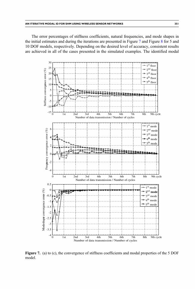
The error percentages of stiffness coefficients, natural frequencies, and mode shapes inthe initial estimates and during the iterations are presented in Figure 7 and Figure 8 for 5 and10 DOF models, respectively. Depending on the desired level of accuracy, consistent resultsare achieved in all of the cases presented in the simulated examples. The identified modal

15

20

25

30

ence

err

or (

%)

-10

-5

0

5

10

Stif

fnes

s co

nver

ge

0 1st 2nd 3rd 4th 5th 6th 7th 8th 9th cycle-15

Number of data transmission / Number of cycles

4

6

erro

r (%

)

-2

0

2

4

uenc

y co

nver

genc

e

0

0.5

or (

%)

0 1st 2nd 3rd 4th 5th 6th 7th 8th 9th cycle

-4


Freq

u

-2.5

-2

-1.5

-1

-0.5

e co

nver

genc

e er

ro

0 1st 2nd 3rd 4th 5th 6th 7th 8th 9th cycle-4

-3.5

-3


Mod

esha

pe

1st floor

2nd floor

3rd floor

4th floor

5th floor

1st mode

2nd mode

3rd modeth4th mode

5th mode

2nd mode2 mode

3rd mode

4th mode

5th mode

1st mode

Figure 7. (a) to (c), the convergence of stiffness coefficients and modal properties of the 5 DOFmodel.


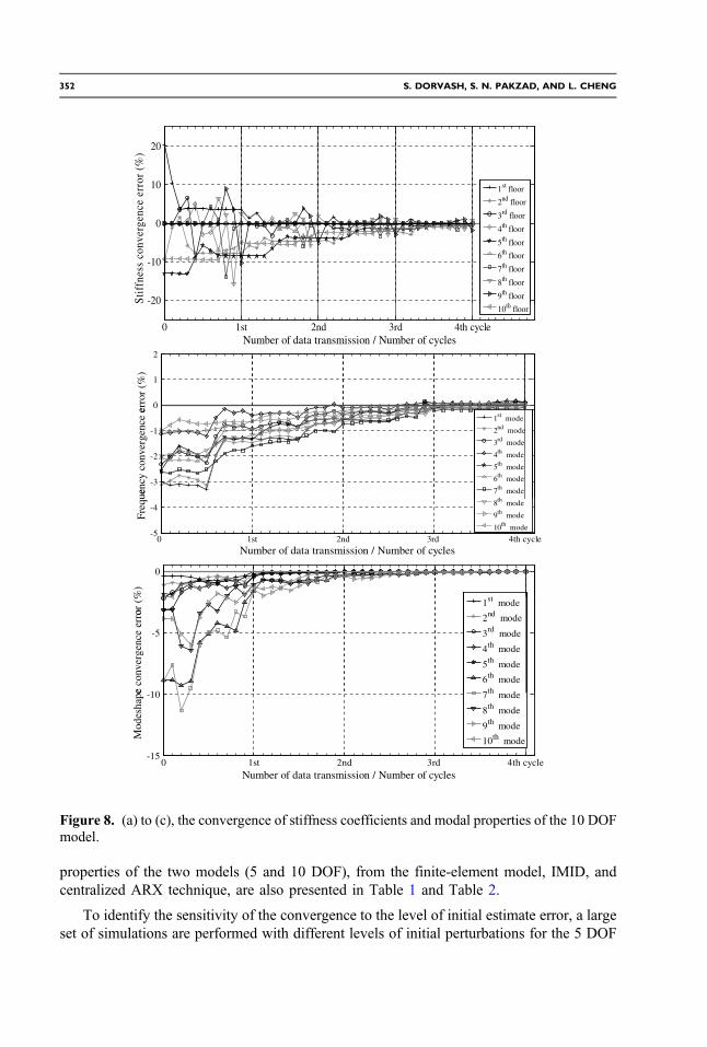
properties of the two models (5 and 10 DOF), from the finite-element model, IMID, andcentralized ARX technique, are also presented in Table 1 and Table 2.

To identify the sensitivity of the convergence to the level of initial estimate error, a largeset of simulations are performed with different levels of initial perturbations for the 5 DOF

10

20nc

e er

ror

(%)

1st floor

2nd floor

-20

-10

0

tiff

ness

con

verg

e 3rd floor

4th floor

5th floor

6th floor

7th floor

8th floor

9th floorth

0 1st 2nd 3rd 4th cycleNumber of data transmission / Number of cycles

S

10th floor

0

1

2

erro

r (%

)

-3

-2

-1

0

ency

con

verg

ence

e

1st mode

2nd mode

3rd mode

4th mode

5th mode

6th mode

7th modeth

0

or (

%)

t

0 1st 2nd 3rd 4th cycle-5

-4


Freq

ue

8th mode

9th mode

10th mode

10

-5

e co

nver

genc

e er

ro

1st mode

2nd mode

3rd mode

4th mode

5th mode

6th mode

7th d

0 1st 2nd 3rd 4th cycle-15

-10


Mod

esha

pe 7th mode

8th mode

9th mode

10th mode

Figure 8. (a) to (c), the convergence of stiffness coefficients and modal properties of the 10 DOFmodel.


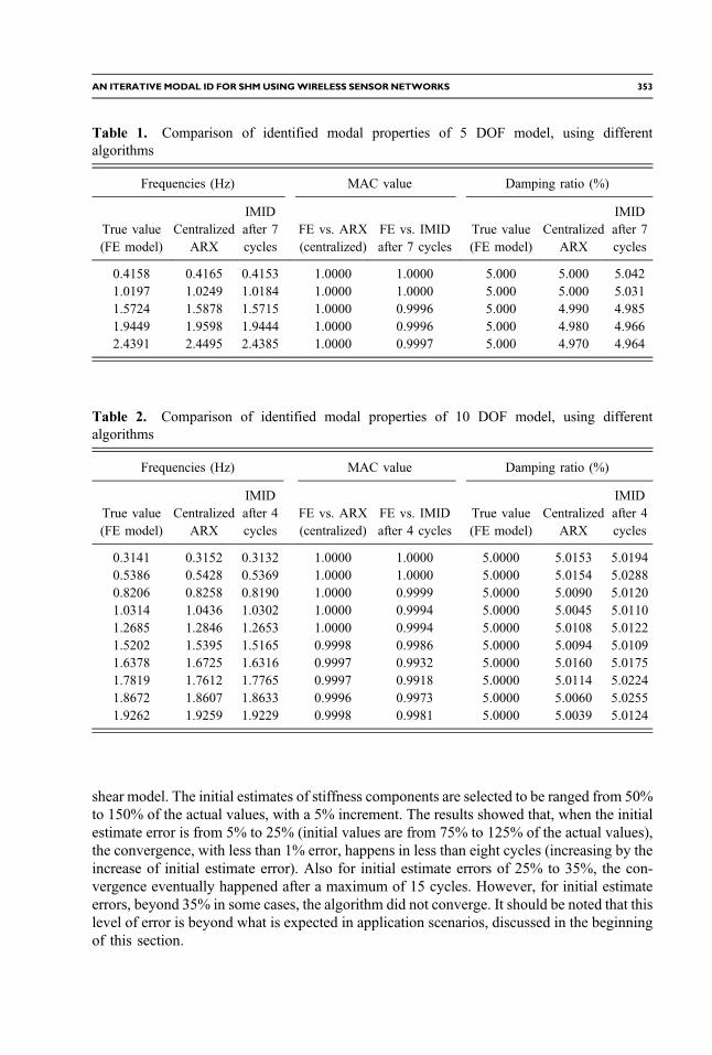
shear model. The initial estimates of stiffness components are selected to be ranged from 50%to 150% of the actual values, with a 5% increment. The results showed that, when the initialestimate error is from 5% to 25% (initial values are from 75% to 125% of the actual values),the convergence, with less than 1% error, happens in less than eight cycles (increasing by theincrease of initial estimate error). Also for initial estimate errors of 25% to 35%, the con-vergence eventually happened after a maximum of 15 cycles. However, for initial estimateerrors, beyond 35% in some cases, the algorithm did not converge. It should be noted that thislevel of error is beyond what is expected in application scenarios, discussed in the beginningof this section.

Table 1. Comparison of identified modal properties of 5 DOF model, using differentalgorithms

Frequencies (Hz) MAC value Damping ratio (%)

True value(FE model)

CentralizedARX

IMIDafter 7cycles

FE vs. ARX(centralized)

FE vs. IMIDafter 7 cycles


CentralizedARX

IMIDafter 7cycles

0.4158 0.4165 0.4153 1.0000 1.0000 5.000 5.000 5.0421.0197 1.0249 1.0184 1.0000 1.0000 5.000 5.000 5.0311.5724 1.5878 1.5715 1.0000 0.9996 5.000 4.990 4.9851.9449 1.9598 1.9444 1.0000 0.9996 5.000 4.980 4.9662.4391 2.4495 2.4385 1.0000 0.9997 5.000 4.970 4.964

Table 2. Comparison of identified modal properties of 10 DOF model, using differentalgorithms

Frequencies (Hz) MAC value Damping ratio (%)


CentralizedARX

IMIDafter 4cycles

FE vs. ARX(centralized)

FE vs. IMIDafter 4 cycles


CentralizedARX

IMIDafter 4cycles

0.3141 0.3152 0.3132 1.0000 1.0000 5.0000 5.0153 5.01940.5386 0.5428 0.5369 1.0000 1.0000 5.0000 5.0154 5.02880.8206 0.8258 0.8190 1.0000 0.9999 5.0000 5.0090 5.01201.0314 1.0436 1.0302 1.0000 0.9994 5.0000 5.0045 5.01101.2685 1.2846 1.2653 1.0000 0.9994 5.0000 5.0108 5.01221.5202 1.5395 1.5165 0.9998 0.9986 5.0000 5.0094 5.01091.6378 1.6725 1.6316 0.9997 0.9932 5.0000 5.0160 5.01751.7819 1.7612 1.7765 0.9997 0.9918 5.0000 5.0114 5.02241.8672 1.8607 1.8633 0.9996 0.9973 5.0000 5.0060 5.02551.9262 1.9259 1.9229 0.9998 0.9981 5.0000 5.0039 5.0124


EXPERIMENTAL VALIDATION OF IMID

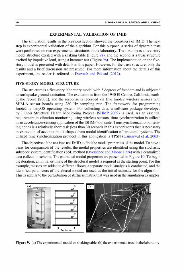
The simulation results in the previous section showed the robustness of IMID. The nextstep is experimental validation of the algorithm. For this purpose, a series of dynamic testswere performed on two experimental structures in the laboratory. The first one is a five-storymodel structure excited with a shaking table (Figure 9a), and the second is a truss structureexcited by impulsive load, using a hammer test (Figure 9b). The implementation on the five-story model is presented with details in this paper. However, for the truss structure, only theresults and a brief discussion are presented. For more information about the details of thisexperiment, the reader is referred to Dorvash and Pakzad (2012).

FIVE-STORY MODEL STRUCTURE

The structure is a five-story laboratory model with 5 degrees of freedom and is subjectedto earthquake ground excitation. The excitation is from the 1940 El Centro, California, earth-quake record (S00E), and the response is recorded via five Imote2 wireless sensors withSHM-A sensor boards using 280 Hz sampling rate. The framework for programmingImote2 is TinyOS operating system. For collecting data, a software package developedby Illinois Structural Health Monitoring Project (ISHMP 2009) is used. As an essentialrequirement in vibration monitoring using wireless sensors, time synchronization is utilizedin an acceleration-sensing application of the ISHMP tool suite. Time synchronization of sens-ing nodes is a relatively short task (less than 30 seconds in this experiment) that is necessaryin extraction of accurate mode shapes from modal identification of structural systems. Theutilized time synchronization protocol in this application is TPSN (Ganeriwal et al. 2003).

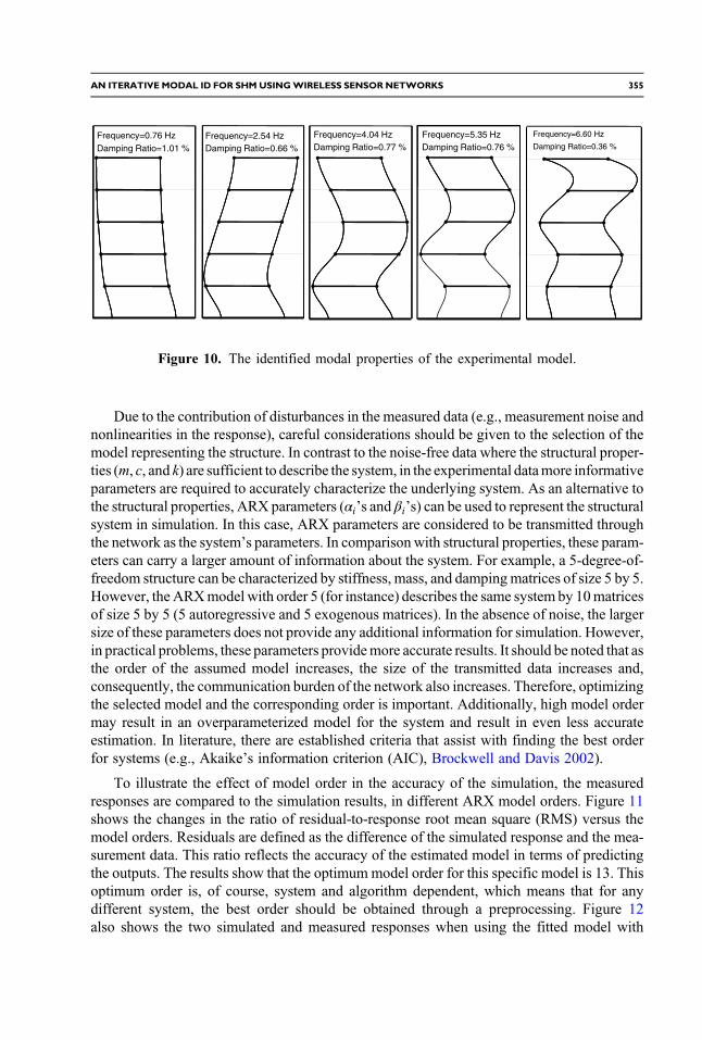
The objective of the test is to use IMID to find themodal properties of themodel. To have abasis for comparison of the results, the modal properties are identified using the stochasticsubspace system identification (SSI) method (Overschee and Moore 1994) with a centralizeddata collection scheme. The estimated modal properties are presented in Figure 10. To beginthe iteration, an initial estimate of the structural model is required as the starting point. For thisexample, masses are added to different floors, a separate modal analysis is conducted, and theidentified parameters of the altered model are used as the initial estimate for the algorithm.This is similar to the perturbation of stiffness matrix that was used in the simulation examples.

(a) (b)

Figure 9. (a) The experimentalmodel on shaking table; (b) the experimental truss in the laboratory.


Due to the contribution of disturbances in the measured data (e.g., measurement noise andnonlinearities in the response), careful considerations should be given to the selection of themodel representing the structure. In contrast to the noise-free data where the structural proper-ties (m, c, and k) are sufficient to describe the system, in the experimental datamore informativeparameters are required to accurately characterize the underlying system. As an alternative tothe structural properties, ARX parameters (αi’s and βi’s) can be used to represent the structuralsystem in simulation. In this case, ARX parameters are considered to be transmitted throughthe network as the system’s parameters. In comparisonwith structural properties, these param-eters can carry a larger amount of information about the system. For example, a 5-degree-of-freedom structure can be characterized by stiffness, mass, and dampingmatrices of size 5 by 5.However, theARXmodel with order 5 (for instance) describes the same system by 10matricesof size 5 by 5 (5 autoregressive and 5 exogenous matrices). In the absence of noise, the largersize of these parameters does not provide any additional information for simulation. However,in practical problems, these parameters providemore accurate results. It should be noted that asthe order of the assumed model increases, the size of the transmitted data increases and,consequently, the communication burden of the network also increases. Therefore, optimizingthe selected model and the corresponding order is important. Additionally, high model ordermay result in an overparameterized model for the system and result in even less accurateestimation. In literature, there are established criteria that assist with finding the best orderfor systems (e.g., Akaike’s information criterion (AIC), Brockwell and Davis 2002).

To illustrate the effect of model order in the accuracy of the simulation, the measuredresponses are compared to the simulation results, in different ARX model orders. Figure 11shows the changes in the ratio of residual-to-response root mean square (RMS) versus themodel orders. Residuals are defined as the difference of the simulated response and the mea-surement data. This ratio reflects the accuracy of the estimated model in terms of predictingthe outputs. The results show that the optimummodel order for this specific model is 13. Thisoptimum order is, of course, system and algorithm dependent, which means that for anydifferent system, the best order should be obtained through a preprocessing. Figure 12also shows the two simulated and measured responses when using the fitted model with

Frequency=0.76 HzDamping Ratio=1.01 %




Frequency=6.60 Hz

Damping Ratio=0.36 %

Figure 10. The identified modal properties of the experimental model.


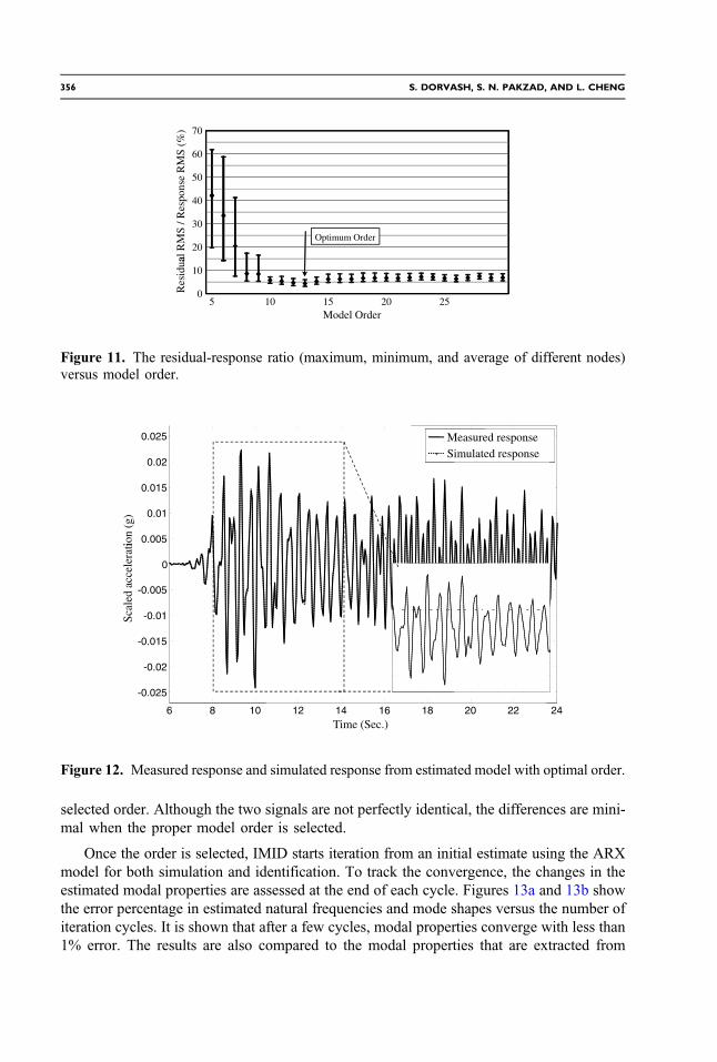
selected order. Although the two signals are not perfectly identical, the differences are mini-mal when the proper model order is selected.

Once the order is selected, IMID starts iteration from an initial estimate using the ARXmodel for both simulation and identification. To track the convergence, the changes in theestimated modal properties are assessed at the end of each cycle. Figures 13a and 13b showthe error percentage in estimated natural frequencies and mode shapes versus the number ofiteration cycles. It is shown that after a few cycles, modal properties converge with less than1% error. The results are also compared to the modal properties that are extracted from

50

60

70

nse

RM

S (%

)

20

30

40

al R

MS

/ Res

po

0

10

5 10 15 20 25

Res

idua

Model Order

Optimum Order

Figure 11. The residual-response ratio (maximum, minimum, and average of different nodes)versus model order.

0.02

0.025 Measured responseSimulated response

0 005

0.01

0.015

0.02

-0.005

0

0.005

-0.02

-0.015

-0.01

6 8 10 12 14 16 18 20 22 24

-0.025

Time (Sec.)

ion

(g)

led

acce

lera

tiSc

a

Figure 12. Measured response and simulated response from estimated model with optimal order.


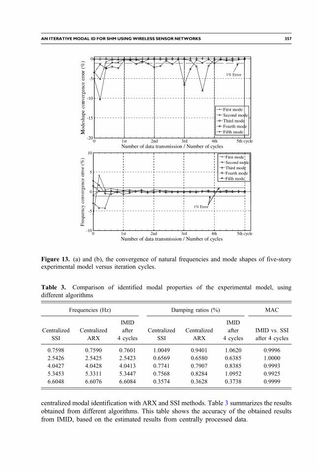
centralized modal identification with ARX and SSI methods. Table 3 summarizes the resultsobtained from different algorithms. This table shows the accuracy of the obtained resultsfrom IMID, based on the estimated results from centrally processed data.

0

or (

%)

-10

-5nv

erge

nce

erro 1% Error

20

-15

Mod

esha

pe c

on

First modeSecond modeThird modeFourth modeFifth mode

0 1st 2nd 3rd 4th 5th cycle-20

M

5

10

rror

(%

) First modeSecond modeThird mode

0

5

conv

erge

nce

er Fourth modeFifth mode

0 1st 2nd 3rd 4th 5th cycle-10

-5

Freq

uenc

y 1% Error



Figure 13. (a) and (b), the convergence of natural frequencies and mode shapes of five-storyexperimental model versus iteration cycles.

Table 3. Comparison of identified modal properties of the experimental model, usingdifferent algorithms

Frequencies (Hz) Damping ratios (%) MAC

CentralizedSSI

CentralizedARX

IMIDafter

4 cyclesCentralized

SSICentralized

ARX

IMIDafter

4 cyclesIMID vs. SSIafter 4 cycles

0.7598 0.7590 0.7601 1.0049 0.9401 1.0620 0.99962.5426 2.5425 2.5423 0.6569 0.6580 0.6385 1.00004.0427 4.0428 4.0413 0.7741 0.7907 0.8385 0.99935.3453 5.3311 5.3447 0.7568 0.8284 1.0952 0.99256.6048 6.6076 6.6084 0.3574 0.3628 0.3738 0.9999


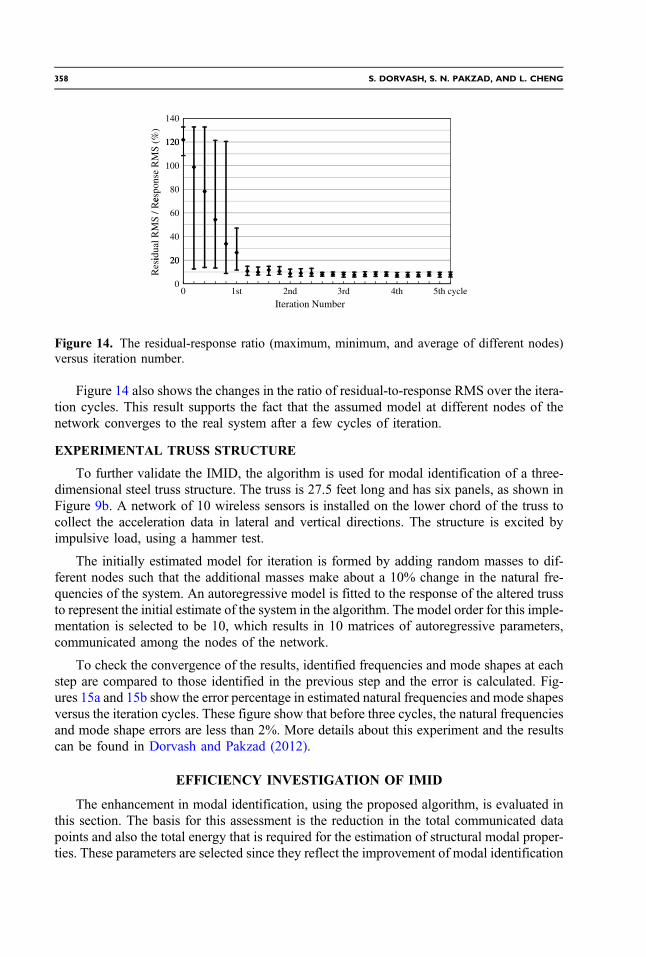
Figure 14 also shows the changes in the ratio of residual-to-response RMS over the itera-tion cycles. This result supports the fact that the assumed model at different nodes of thenetwork converges to the real system after a few cycles of iteration.

EXPERIMENTAL TRUSS STRUCTURE

To further validate the IMID, the algorithm is used for modal identification of a three-dimensional steel truss structure. The truss is 27.5 feet long and has six panels, as shown inFigure 9b. A network of 10 wireless sensors is installed on the lower chord of the truss tocollect the acceleration data in lateral and vertical directions. The structure is excited byimpulsive load, using a hammer test.

The initially estimated model for iteration is formed by adding random masses to dif-ferent nodes such that the additional masses make about a 10% change in the natural fre-quencies of the system. An autoregressive model is fitted to the response of the altered trussto represent the initial estimate of the system in the algorithm. The model order for this imple-mentation is selected to be 10, which results in 10 matrices of autoregressive parameters,communicated among the nodes of the network.

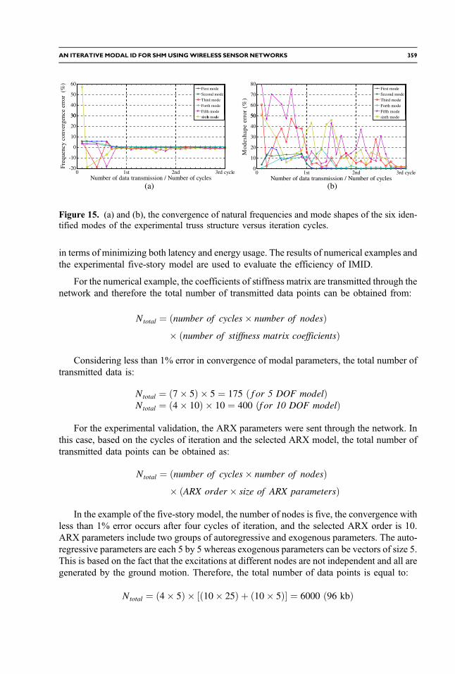
To check the convergence of the results, identified frequencies and mode shapes at eachstep are compared to those identified in the previous step and the error is calculated. Fig-ures 15a and 15b show the error percentage in estimated natural frequencies and mode shapesversus the iteration cycles. These figure show that before three cycles, the natural frequenciesand mode shape errors are less than 2%. More details about this experiment and the resultscan be found in Dorvash and Pakzad (2012).

EFFICIENCY INVESTIGATION OF IMID

The enhancement in modal identification, using the proposed algorithm, is evaluated inthis section. The basis for this assessment is the reduction in the total communicated datapoints and also the total energy that is required for the estimation of structural modal proper-ties. These parameters are selected since they reflect the improvement of modal identification

0 1st 2nd 3rd 4th 5th cycle

Iteration Number

120

140

%)

80

100

120es

pons

e R

MS

(

20

40

60

idua

l RM

S / R

e

0

20

Res

i

Figure 14. The residual-response ratio (maximum, minimum, and average of different nodes)versus iteration number.


in terms of minimizing both latency and energy usage. The results of numerical examples andthe experimental five-story model are used to evaluate the efficiency of IMID.

For the numerical example, the coefficients of stiffness matrix are transmitted through thenetwork and therefore the total number of transmitted data points can be obtained from:

EQ-TARGET;temp:intralink-;sec7;62;405Ntotal ¼ ðnumber of cycles� number of nodesÞ� ðnumber of stiffness matrix coefficientsÞ

Considering less than 1% error in convergence of modal parameters, the total number oftransmitted data is:

EQ-TARGET;temp:intralink-;sec7;62;325

Ntotal ¼ ð7� 5Þ � 5 ¼ 175 ð f or 5 DOF modelÞNtotal ¼ ð4� 10Þ � 10 ¼ 400 ðf or 10 DOF modelÞ

For the experimental validation, the ARX parameters were sent through the network. Inthis case, based on the cycles of iteration and the selected ARX model, the total number oftransmitted data points can be obtained as:

EQ-TARGET;temp:intralink-;sec7;62;245Ntotal ¼ ðnumber of cycles� number of nodesÞ� ðARX order � size of ARX parametersÞ

In the example of the five-story model, the number of nodes is five, the convergence withless than 1% error occurs after four cycles of iteration, and the selected ARX order is 10.ARX parameters include two groups of autoregressive and exogenous parameters. The auto-regressive parameters are each 5 by 5 whereas exogenous parameters can be vectors of size 5.This is based on the fact that the excitations at different nodes are not independent and all aregenerated by the ground motion. Therefore, the total number of data points is equal to:

EQ-TARGET;temp:intralink-;sec7;62;121Ntotal ¼ ð4� 5Þ � ½ð10� 25Þ þ ð10� 5Þ� ¼ 6000 ð96 kbÞ

30

40

50

60First modeSecond mode

Third mode

Forth mode

Fifth modei h d 50

60

70

80First modeSecond modeThird modeForth modeFifth mode

0

10

20

30 sixth mode

20

30

40

50

Mod

esha

pe e

rror

(%

)

sixth mode

0 1st 2nd 3rd cycle-20

-10


Freq

uenc

y co

nver

genc

e er

ror

(%

)

0 1st 2nd 3rd cycle0

10

Number of data transmission / Number of cycles(a) (b)

Figure 15. (a) and (b), the convergence of natural frequencies and mode shapes of the six iden-tified modes of the experimental truss structure versus iteration cycles.


The efficiency of IMID becomes clearer when comparing this approach with the cen-tralized computation method. For centralized computation, the data needs to be transferredto the base station. To transfer the collected data, sensors can either send their data directly tothe base station (centralized data collection scheme, Figure 16a) or send them through theintermediary nodes, called multihop communication (Figure 16b). Use of multihop datatransmission is essential when the network is long and there are nodes that are not in theradio range of the base station (e.g., implementation of WSN on long-span bridges).When using the centralized data transmission routing, the total number of data pointswill be simply N:ns where ns is the number of sensors and N is the number of collecteddata points at each sensor. Also, in multihop communication routing, the total transmitteddata is N:nsðns þ 1Þ∕2 (Pakzad et al. 2008). In modal identification process, the higher thenumber of collected data samples is, the better the estimation of modal properties would be.In this implementation, 25,000 samples were collected at each sensor node. Considering useof centralized data transmission, 125,000 (2,000 kb) will be the total samples need to becommunicated. In multihop data transmission and routing, which is essential in many wire-less sensor network deployments, the significance of the proposed algorithm will be evenmore evident, as such implementations need ðns þ 1Þ∕2 times larger transmission when col-lecting the data at the base station, but the same when using the IMID approach.

COMPARISON OF THE TOTAL ENERGY

Considering the results and specifications of the experimental implementation, the energyconsumed by the two approaches, namely IMID and centralized system identification, areestimated and compared.

Required energy for data transmission can be calculated simply from Equation 2 by hav-ing the volume of the data, the transmission rate, and the power consumption rate:

EQ-TARGET;temp:intralink-;sec7.1;41;201Etrsmission ¼ ½1∕transmission rate ðKbpsÞ� � ½power consumption rate ðmWÞ�

where the nominal transmission rate of the embedded transceiver on Imote2 is 250 kbps(Crossbow 2007) and the power consumption rate, while transmitting the data, is245 mW (Figure 2).

Estimating the required energy for data processing is more challenging since it needs anestimate of computation time. Chang and Pakzad (2012) conducted a comprehensive studyon the required computational time for several different time domain system identification

Figure 16. (a) The centralized data transmission routing; (b) multihop data transmission routing.


algorithms. In this study the required number of operations is presented as a function ofmodel order, number of outputs, and signal length. Then the computation times in differentalgorithms are presented and compared. It is concluded through simulated examples that thetotal consumed time for performing the entire identification process for a system with 5 out-puts and order of 10 is just a fraction of second (less than 0.1 second).

The computational time for the numerical simulation of the response, using an ARXmodel, is also measured for the 5-degree-of-freedom system of the presented exampleand resulted in less than 0.05 seconds of CPU time. Considering these estimations of com-putational time at each node, four cycles of iteration, and 184 mW power consumption rate(Figure 2) of the Imote2 in data processing mode (radio off), the consumed power for com-putation is about 400 mW/sec. Also, the required energy for transmission of 96 kb data, usingEquation 2, will be about 94 mW/sec, which results in 494 mW/sec total energy.

For application of the centralized data processing to this example, considering the transferof 2,000 kb of data, the total required energy will be 1960 mW/sec.

This estimation shows a 75% savings in the consumed energy for IMID versus thecentralized method. However, a few important considerations should be noted. First, thecomputational time may increase depending on the microcontroller that is responsible foron-board processing. If high performance processors are utilized in the next generationsof wireless sensor units, this processing time can further decrease for the decentralize ana-lysis. Second, the transmission rate considered in this study is the nominal rate presented inthe data sheet of the CC2440 transceiver. However, in practice the actual transmission ratesare less since there is a communication overhead due to packet loss and collisions in thewireless communication (e.g., see Nagayama et al. 2010, which reported a maximum 83kbps communication rate in single-hop transmission in laboratory experiments). A lowercommunication rate causes a higher energy demand for the data transmission task, whichadversely affects the centralized processing methods disproportionately. Third, in these esti-mations, it is assumed that the transmission scheme is centralized and single-hop. The use ofmultihop data transmission results in a longer data collection time. Therefore, the benefits ofIMID will be more significant when a multihop data transmission scheme is utilized.

In comparing the required data transmission and energy consumption for IMID withthose of centralized processing methods, it is evident that a substantial reduction in the net-work communication and the total consumed energy is achieved. Complete comparison withother decentralized system identification methods (e.g., Pakzad et al. 2011, Sim and Spencer2009, Sim et al. 2010, Nagayama and Spencer 2007) may not be possible, since unlike thosemethods, IMID is an iterative process and the total computation/communication cost dependson how fast convergence could happen. The simulated and experimental results presented inthis paper shows significant improvement in both agility and energy efficiency of the sensornetwork.

CONCLUSION

This paper presents a new distributed modal identification algorithm, called IMID, toaddress challenges in the application of wireless sensor networks in health monitoringof structural systems. The proposed algorithm is structured similar to iterative expecta-tion-maximization series of algorithms that estimate unknown parameters in the presence


of hidden information. The main objective in developing such an algorithm is to reduce thecommunication burden in WSN as a smart way of saving computation time and communica-tion power. Latency and energy consumption are two factors that prevent WSNs from promptresponse to earthquake events and also restrict their application in long-term monitoring. Theproposed algorithm achieves significant reduction in the total transmitted data by incorpor-ating the on-board computational capability of wireless sensors. To verify the performance ofIMID, two numerically simulated models and two experimental models are used as the imple-mentation test beds. The results illustrate the convergence of modal parameters after a fewiteration cycles.

The advantage of IMID is its flexibility in collaboration with a broad range of identifica-tion and simulation algorithms. In this implementation, Newmark’s numerical method andautoregressive with exogenous algorithms are used for simulation and identification steps.Further studies are required to evaluate the efficiency of IMID if other methods are used forthese steps.

The application of this algorithm is particularly beneficial in long-term structural healthmonitoring in which the current state of the system can be considered as the initial estimate.These modal parameters are updated using data collected during the monitoring period. Hav-ing the identified modal properties of the system in a long period of time, applications such asdamage detection and/or finite-element model updating can be utilized in the system as well.

ACKNOWLEDGMENTS

The research described in this paper is supported by the National Science Foundationthrough grant no. CMMI-0926898 by Sensors and Sensing Systems Program and by agrant from the Commonwealth of Pennsylvania, Department of Community and EconomicDevelopment, through the Pennsylvania Infrastructure Technology Alliance (PITA).

REFERENCES

Brockwell, P. J., and Davis, R. A., 2002. Introduction to Time Series and Forecasting,2nd edition, Springer, New York.

Brownjohn, J. M. W., and Xia, P. Q., 2000. Dynamic assessment of curved cable-stayed bridgeby model updating, Journal of Structural Engineering 126, 252–260.

Caffrey, J., Govindan, R., Johnson, E., Krishnamachari, B., Masri, S., Sukhatme, G.,Chintalapudi, K., Dantu, K., Rangwala, S., Sridharan, A., Xu, N., and Zuniga, M., 2004.Networked sensing for structural health monitoring, Proceedings of the 4th InternationalWorkshop on Structural Control, New York, NY, 10–11 June, 57–66.

Chang, M., and Pakzad, S. N., 2012. Modified natural excitation technique for stochastic modelidentification, Journal of Structural Engineering, doi:10.1061/(ASCE)ST.1943-541X.0000559.

Chipcon AS SmartRF®, 2004. CC2420 Preliminary Datasheet, rev 1.2.Cho, S., Jo, H., Jang, S., Park, J., Jung, H.J., Yun, C.B., Spencer, Jr., B. F., and Seo, J., 2010.

Structural health monitoring of a cable-stayed bridge using smart sensor technology: Dataanalysis, Smart Structures and Systems 6, 461–480.

Chung, H. C., Enotomo, T., Loh, K., and Shinozuka, M., 2004. Real-time Visualization of bridgestructural response through wireless MEMS sensors, Proceedings of SPIE, Testing,


http://dx.doi.org/10.1061/(ASCE)0733-9445(2000)126:2(252)

http://dx.doi.org/10.1061/(ASCE)ST.1943-541X.0000559

Reliability, and Application of Micro- and Nano-Material Systems II, San Diego, CA,Vol. 5392, 239–246.

Crossbow, 2007. Imote2, high-performance wireless sensor network node, Product data sheet,http://www.xbow.com.

Das, N. K., Khorrami, F., and Nourbakhsh, S., 1998. A new integrated piezoelectric–dielectricmicrostrip antenna for dual wireless actuation and sensing functions, Proceedings of the SPIE,Smart Electronics and MEMS, San Diego, CA, Vol. 3328, 133–146.

Dempster, A. P., Laird, N. M., and Rubin, D. B., 1997. Maximum likelihood from incompletedata via the EM algorithm, Journal of Royal Statistical Society, Series B (Methodological), 39,1–38.

Dorvash, S., and Pakzad, S. N., 2012. Iterative modal identification algorithm: Implementationand evaluation, in Proceedings of the 30th International Modal Analysis Conference (IMACXXX), Jacksonville, FL, 30 January–2 February.

Ganeriwal, S., Kumar, R., and Srivastava, M. B., 2003. Timing-sync protocol for sensor net-works. UC Los Angeles: Center for Embedded Network Sensing, http://escholarship.org/uc/item/5mh7m01j.

Gao, Y., Spencer, Jr., B. F., and Ruiz-Sandoval, M., 2006. Distributed computing strategyfor structural health monitoring, Journal of Structural Control and Health Monitoring 13,488–507.

Grisso, B. L., Martin, L. A., and Inman, D. J., 2005. A wireless active sensing system forimpedance-based structural health monitoring, Proceedings of the 23rd InternationalModal Analysis Conference, Orlando, FL.

Hackmann, G., Sun, F., Castaneda, N., Chenyang Lu, and Dyke, S., 2008. A holistic approach todecentralized structural damage localization using wireless sensor networks, Real-TimeSystems Symposium, Barcelona, Spain, 30 November–3 December, 35–46.

Illinois Structural Health Monitoring Project (ISHMP), 2009. ISHMP Services Toolsuite, http://shm.cs.uiuc.edu/software.html.

Jang, S., Jo, H., Cho, S., Mechitov, K., Rice, J. A., Sim, S. H., Jung, H. J., Yun, C. B., Spencer,Jr., B. F., and Agha, G., 2010. Autonomous structural health monitoring using wireless smartsensors on a cable-stayed bridge, Proceedings of the Fifth International IABMAS Conference,Philadelphia, 11- July 2010, CRC Press.

Kim, J., Swartz, R. A., Lynch, J. P., Lee, J. J., and Lee, C. G., 2010. Rapid-to-Deploy reconfi-gurable wireless structural monitoring systems using extended-range wireless sensors, SmartStructures and Systems 6, 505–524.

Liu, S. C., and Tomizuka, M., 2003. Strategic research for sensors and smart structures technol-ogy, Proceedings of the International Conference on Structural Health Monitoring and Intel-ligent Infrastructure, Tokyo, Japan, 13–15 November, vol. 1, 113–117.

Lynch, J. P., Sundararajan, A., Law, K. H., Kiremidjian, A. S., and Carryer, E., 2003. Power-efficient data management for a wireless structural monitoring system, Proceedings of the 4thInternational Workshop on Structural Health Monitoring, Stanford, CA, 15–17 September,1177–1184.

Lynch, J. P., Law, K. H., Kiremidjian, A. S., Carryer, E., Farrar, C. R., Sohn, H., Allen, D. W.,Nadler, B., and Wait, J. R., 2004a. Design and performance validation of a wirelesssensing unit for structural monitoring application, Structural Engineering and Mechanics,An International Journal, 17, 393–408.


http://www.xbow.com

http://www.xbow.com

http://www.xbow.com

http://escholarship.org/uc/item/5mh7m01j



http://dx.doi.org/10.1002/(ISSN)1545-2263

http://shm.cs.uiuc.edu/software.html






Lynch, J. P., Sundararajan, A., Law, K. H., Kiremidjian, A. S., and Carryer, E., 2004b. Embed-ding damage detection algorithms in a wireless sensing unit for operational power efficiency,Smart Materials and Structures 13, 800–810.

Lynch, J. P., Wang, Y., Law, K. H., Yi, J-H., Lee, C. G., and Yun, C. B., 2005. Validation of alarge-scale wireless structural monitoring system on the Geumdang Bridge, Proceedings of theInternational Conference on Safety and Structural Reliability (ICOSSAR), Rome, Italy, 19–23June.

The Math Works, Inc., 1997. MATLAB and Simulink, Natick, MA.Moon, T. K., 1996. The expectation maximization algorithm in signal processing, IEEE Signal

Processing Magazine 13, 47–60. DOI 10.1109/79.543975.Nagayama, T., Moinzadeh, P., Mechitov, K., Ushita, M., Makihata, N., Ieiri, M., Agha, G.,

Spencer, Jr., B. F., Fujino, Y., and Seo, J. W., 2010. Reliable multi-hop communicationfor structural health monitoring, Smart Structures and Systems 6, 481–504.

Nagayama, T., and Spencer, Jr., B. F., 2007. Structural health monitoring using smart sensors,Newmark Structural Engineering Laboratory (NSEL) Report Series No. 1, University of Illi-nois at Urbana-Champaign, Urbana, Illinois, http://hdl.handle.net/2142/3521.

Overschee, P. V., and Moor, B. D., 1994. N4SID: Subspace algorithms for the identification ofcombined deterministic-stochastic systems, Automatica 30, 75–93.

Pakzad, S. N., 2010. Development and deployment of large scale wireless sensor network on along-span bridge, Smart Structures and Systems 6, 525–543.

Pakzad, S. N., Fenves, G. L., Kim, S., and Culler, D. E., 2008. Design and implementation ofscalable wireless sensor network for structural monitoring, Journal of Infrastructure Systems14, 89–101.

Pakzad, S. N., Rocha, G. V., and Yu, B., 2011. Distributed modal identification using restrictedauto regressive models, International Journal of Systems Science 42, 1473–1489. doi:10.1080/00207721.2011.563875.

Pandit, S. M., 1991.Modal and Spectrum Analysis: Data Dependent Systems in State Space, JohnWiley and Sons.

Pappa, R. S., James, G. H., and Zimmerman, D. C., 1997. Autonomous modal identification ofthe space shuttle tail rudder, NASA Technical Memorandum, Hampton, VA, 12 pp.

Peeters, B., and Roeck, G. D., 2001. Stochastic system identification for operational modalanalysis: A review, Journal of Dynamic Systems, Measurement, and Control 123, 659–667.

Rice, J. A., and Spencer, Jr., B. F., 2008. Structural health monitoring sensor development for theImote2 platform, Proceedings of SPIE Smart Structures/NDE, San Diego, CA, doi:10.1117/12.776695

Roeck, G. D., Claesen, W., and Broeck, P. V. D., 1995. DDS-methodology applied to parameteridentification in civil engineering structures, Proceedings of Vibration and Noise, Venice,Italy, 341–353.

Sadhu, A., Bo, H., and Narasimhan, S., 2012. Blind source separation towards decentralizedmodal identification using compressive sampling, in Proceeding of 11th InternationalConference on Information Science, Signal Processing and their Applications (ISSPA),1147–1152.

Sim, S. H., Carbonell-Marquez, J., Spencer, Jr., B. F., and Jo, H., 2010. Decentralized randomdecrement technique for efficient data aggregation and system identification in wireless smartsensor networks, Probabilistic Engineering Mechanics 26, 81–91.


http://dx.doi.org/10.1088/0964-1726/13/4/018

http://dx.doi.org/10.1109/79.543975

http://dx.doi.org/10.1109/79.543975

http://hdl.handle.net/2142/3521



http://dx.doi.org/10.1016/0005-1098(94)90230-5

http://dx.doi.org/10.1080/00207721.2011.563875

http://dx.doi.org/10.1115/1.1410370

http://dx.doi.org/10.1117/12.776695

http://dx.doi.org/10.1016/j.probengmech.2010.07.002

Sim, S. H., and Spencer, B. F., 2009. Decentralized strategies for monitoring structures usingwireless smart sensor networks, NSEL Report Series, http://hdl.handle.net/2142/14280.

Swartz, R. A., Jung, D., Lynch, J. P., Wang, Y., Shi, D., and Flynn, M. P., 2005. Design of awireless sensor for scalable distributed in-network computation in a structural health monitor-ing system, Proceedings of the 5th International Workshop on Structural Health Monitoring,Stanford, CA.

Tanner, N. A., Wait, J. R., Farrar, C. R., and Sohn, H., 2003. Structural health monitoring usingmodular wireless sensors, Journal of Intelligent Material Systems and Structures 14, 43–56.

TinyOS, 2006. http://www.tinyos.net.Whelan, M. J., and Janoyan, K. D., 2009. Design of a robust, high-rate wireless sensor network

for static and dynamic structural monitoring, Journal of Intelligent Material Systems andStructures 20, 849–863.

Zhang, Q. W., Chang, T. Y. P., and Chang, C. C. 2001. Finite-element model updating for theKap Shui Mun cable-stayed bridge, Journal of Bridge Engineering 6, 285–293.

(Received 1 August 2011; accepted 1 March 2012)





http://dx.doi.org/10.1177/1045389X03014001005

http://www.tinyos.net



http://dx.doi.org/10.1177/1045389X08098768

http://dx.doi.org/10.1177/1045389X08098768

http://dx.doi.org/10.1061/(ASCE)1084-0702(2001)6:4(285)