

Analysis of influence of design factors in Eco-efficiency of
the Injection Moulding Process
Rita de Vitória Pereira Nogueira Bravo
Thesis to obtain the Master of Science Degree in
Mechanical Engineering
Supervisors: Prof. Paulo Miguel Nogueira Peças
Prof. Inês Esteves Ribeiro
Examination Committee
Chairperson: Prof. Rui Manuel dos Santos Oliveira Baptista
Supervisor: Prof. Inês Esteves Ribeiro
Members of the Committee: Prof. Elsa Maria Pires Henriques
Eng. Eduardo João de Almeida e Silva
November 2015

ii

iii
Acknowledgments
First of all I would like to express by sincere gratitude to Prof. Paulo Peças and Prof. Inês Ribeiro for
their guidance, patience and understanding in the development of this dissertation.
Secondly, my thanks to all my friends and colleagues, Maria, Mário, Gonçalo, Eliseu, Miguel, Zé,
Carrelha, Jota and Vasco, for their support and friendship throughout this journey and to Mariana, my
dissertation and lunch mate.
Last but not least, to my parents and brother for their continuous encouragement and support, and a
special thanks to my grandmother who, unfortunately, could not witness the end of this adventure but
who always gave me her complete support in all my decisions.

iv
Resumo
O termo Eco-eficiência incide sobre o ambiente e economia, relacionando valor do produto/serviço
com o impacte ambiental através de Rácios de Eco-eficiência. O presente trabalho consiste em
aplicar este conceito ao processo de injeção de plásticos, de acordo com as directrizes do World
Business Council for Sustainable Development, criando uma ferramenta de decisão na fase de design
do molde. Analisando Eco-eficiência numa fase mais inicial do ciclo de produção, fase de design do
molde, é possível diminuir o esforço financeiro, por parte das empresas, na redução de custos de
produção e impacte ambiental, na produção das peças.
De modo a calcular os Rácios de Eco-eficiência foi desenvolvido um Modelo de Processo, baseado
na metodologia ciclo de vida, criando um inventário de recursos e, assim, calculando os custos,
através de um Modelo de Custo Baseado no Processo, e o impacte ambiental.
Os resultados deste modelo são apresentados para diferentes alternativas de designs de molde,
considerando diferentes números de cavidades, tipos de sistema de alimentação e máquinas, e
analisados em termos de recursos, custos, impacte ambiental e Rácios de Eco-eficiência,
demonstrando o raciocínio por trás dos resultados, e comparando estes resultados entre as
alternativas para uma determinada peça e volume de produção.
Este modelo permite também uma análise de sensibilidade ao volume de produção, verificando a
melhor alternativa em termos de custo entre várias alternativas de molde, e a parâmetros da peça,
neste caso a espessura, em termos de custo e impacto ambiental, para uma única alternativa de
molde.
Palavras-Chave: Eco-eficiência; Injecção de Plásticos; Modelo de Processo; Modelo de Custo
Baseado no Processo; Impacte Ambiental; Design de Molde.

v
Abstract
The term Eco-efficiency focuses on the environment and economy, relating service/product value to
the environmental impact through Eco-efficiency Ratios. The present work consists in applying this
concept to the Injection Moulding Process, following the guidelines specified by the World Business
Council for Sustainable Development, creating a tool for decision making in the mould design phase.
Analysing Eco-efficiency in an early stage of the production cycle, the mould design phase, companies
can reduce the financial effort in decreasing production costs and environmental impact in the
production of plastic parts.
To calculate the Eco-efficiency Ratios it is developed a Process Based Model, based on Life Cycle
Engineering methodology, creating a resource inventory and calculating costs, through a Process
Based Cost Model, and environmental impact.
The results of this model are presented for different mould design alternatives, considering a different
number of cavities, type of feeding system and injection machines, and analysed in terms of
resources, costs, environmental impact and Eco-efficiency Ratios, demonstrating the reasoning
behind the results, and comparing these results between alternatives for one part and production
volume.
This model also allows for a sensitivity analysis in terms of production volume, verifying the best
alternative in terms of cost between several mould design alternatives, and of part parameters, in this
case thickness, in terms of cost and environmental impact, for only one mould design alternative.
Keywords: Eco-efficiency; Injection Moulding; Process Based Model; Process Based Cost Model;
Environmental Impact; Mould Design.

vi
Contents
1 Introduction ..................................................................................................................................... 1
2 Plastic Injection Moulding ................................................................................................................ 3
2.1 Technology on a global scale ................................................................................................. 3
2.2 Process description ................................................................................................................ 4
2.2.1 Moulding cycle ................................................................................................................... 4
2.2.2 Injection Machine ............................................................................................................... 5
2.2.3 Mould ................................................................................................................................. 6
2.2.4 Materials for injection moulding .......................................................................................... 8
2.3 Process analysis – variables and their influence in process performance .............................. 8
3 Performance evaluation in a Life Cycle Perspective ..................................................................... 12
3.1 Historical evolution of sustainability ...................................................................................... 12
3.2 Methodologies and approaches for performance analysis in a life cycle perspective ........... 14
3.2.1 Life Cycle Engineering (LCE) ........................................................................................... 14
3.2.2 Life Cycle Assessment (LCA) ........................................................................................... 15
3.2.3 Life Cycle Cost Analysis (LCC) ........................................................................................ 16
3.3 Eco-efficiency ....................................................................................................................... 18
3.3.1 Philosophy and Principles ................................................................................................ 18
3.3.2 Performance Measure and Indicators .............................................................................. 19
3.3.3 Application in different industry sectors ............................................................................ 22
3.3.4 Application in the plastic and moulding sector.................................................................. 23
4 Methodology for Model Development and Results Analysis .......................................................... 27
5 Process Based Model ................................................................................................................... 30
5.1 Process Flowchart ................................................................................................................ 30
5.2 Process Based Cost Model .................................................................................................. 32
5.2.1 Model Development ......................................................................................................... 34
5.2.2 Model Validation ............................................................................................................... 45
5.3 Process Based Environmental Impact .................................................................................. 48
6 Results .......................................................................................................................................... 50
6.1 Process Based Model Results .............................................................................................. 50
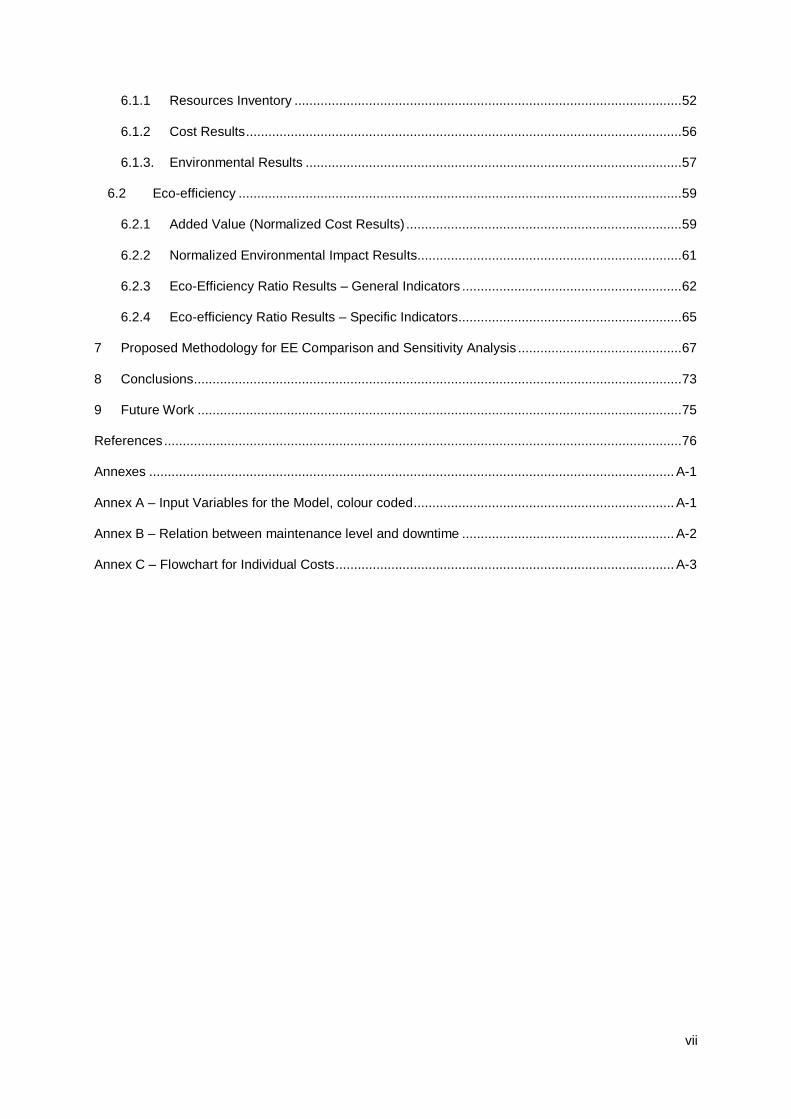
vii
6.1.1 Resources Inventory ........................................................................................................ 52
6.1.2 Cost Results ..................................................................................................................... 56
6.1.3. Environmental Results ..................................................................................................... 57
6.2 Eco-efficiency ....................................................................................................................... 59
6.2.1 Added Value (Normalized Cost Results) .......................................................................... 59
6.2.2 Normalized Environmental Impact Results....................................................................... 61
6.2.3 Eco-Efficiency Ratio Results – General Indicators ........................................................... 62
6.2.4 Eco-efficiency Ratio Results – Specific Indicators ............................................................ 65
7 Proposed Methodology for EE Comparison and Sensitivity Analysis ............................................ 67
8 Conclusions ................................................................................................................................... 73
9 Future Work .................................................................................................................................. 75
References ........................................................................................................................................... 76
Annexes ............................................................................................................................................. A-1
Annex A – Input Variables for the Model, colour coded ...................................................................... A-1
Annex B – Relation between maintenance level and downtime ......................................................... A-2
Annex C – Flowchart for Individual Costs ........................................................................................... A-3

viii
Figures Index
Figure 2.1 – Typical Injection Moulding Cycle [14] ................................................................................. 4
Figure 2.2 - Injection Moulding Machine [15] .......................................................................................... 5
Figure 2.3 – Mould Example [16] ............................................................................................................ 7
Figure 2.4 - Energy Consumption in Injection Machine [23] ................................................................... 9
Figure 2.5 - Comparison of moulded parts wall thickness with different materials [23] ........................ 11
Figure 3.1 - Three main aspects of Sustainability [26] .......................................................................... 13
Figure 3.2 - Keywords of LCE [32] ....................................................................................................... 15
Figure 3.3 - Revised LCA framework [31]............................................................................................. 16
Figure 3.4 - Life Cycle Cost Analysis Procedure [38] ........................................................................... 17
Figure 3.5 - Process-Based Cost Modelling [30] .................................................................................. 17
Figure 3.6 - Relative Cost of Design Change with Time [12] ................................................................ 23
Figure 3.7 - Breakdown of different fixed and variable cost factors for a typical injection moulding
process [51] .......................................................................................................................................... 26
Figure 4.1 – Methodology for Model Development and Result Analysis .............................................. 29
Figure 5.1 - Macro Flowchart of Injection Moulding Process Inputs and Outputs ................................. 31
Figure 5.2 - Conceptual decomposition of a process based cost model [56]........................................ 33
Figure 5.3 - Colour Code for Model Data.............................................................................................. 35
Figure 5.4 - Material Cost ..................................................................................................................... 36
Figure 5.5 - Energy Cost ...................................................................................................................... 40
Figure 5.6 - Tool Cost ........................................................................................................................... 44
Figure 5.7 - Housing Cover [32] ........................................................................................................... 46
Figure 5.8 - Environmental Impact Flowchart ....................................................................................... 49
Figure 6.1 - Part Design [16] ................................................................................................................ 51
Figure 6.2 - Material quantity breakdown: (a) kg per part and (b) kg per cycle..................................... 53
Figure 6.3 - Cycle time: (a) time per part and (b) time per cycle ........................................................... 54
Figure 6.4 - Energy consumption breakdown: (a) kWh per part and (b) kWh per cycle ....................... 55
Figure 6.5 – Cost Breakdown for design alternatives ........................................................................... 56
Figure 6.6 - Environmental Impact Breakdown ..................................................................................... 58
Figure 6.7 - 𝐼𝐺𝑉𝐴 Results (normalized) for the various alternatives ..................................................... 60

ix
Figure 6.8 - 𝐼𝑁𝑉𝐴 Results (normalized) for the various alternatives ..................................................... 60
Figure 6.9 - Environmental Impact Results (normalized) for the various alternatives ........................... 61
Figure 6.10 – Normalized Eco-Efficiency Results for 𝐼𝐺𝑉𝐴 Results ..................................................... 62
Figure 6.11 - 𝐼𝐺𝑉𝐴 (normalized) vs. Environmental Impact (normalized) ............................................. 63
Figure 6.12 – Normalized Eco-Efficiency Results for 𝐼𝑁𝑉𝐴 Results ..................................................... 64
Figure 6.13 - 𝐼𝑁𝑉𝐴 (normalized) vs. Environmental Impact (normalized) ............................................. 65
Figure 6.14 - Eco-Efficiency Results for Specific Indicators: a) Annual Required Time; b) Energy and
c) Material Waste ................................................................................................................................. 66
Figure 7.1 – Proposed Methodology for EE Comparison ..................................................................... 69
Figure 7.2 – Variation of Cost per part with the Production Volume ..................................................... 70
Figure 7.3 - Variation of Cost per part with Part Thickness for 2,000,000 parts and alternative 4E-H .. 71
Figure 7.4 – Variation of Total Environmental Impact with Part Thickness for 2,000,000 parts and
alternative 4E-H .................................................................................................................................... 72
Figure A.1 - Input Variables for PBCM ............................................................................................... A-1
Figure B.1 - Example of an empirical relation between design characteristics, maintenance level and
downtime. SG – Simple Geometry, CG – Complex Geometry, Abras. Mat. – Abrasive part material
[32] ..................................................................................................................................................... A-2
Figure C.1 - Thermodynamic Energy ................................................................................................. A-3
Figure C.2 - Machine Energy .............................................................................................................. A-4
Figure C.3 - Labour Cost .................................................................................................................... A-5
Figure C.4 - Machine Cost.................................................................................................................. A-6
Figure C.5 - Building Cost .................................................................................................................. A-7
Figure C.6 - Maintenance Cost ........................................................................................................... A-8

x
Tables Index
Table 2.1 – Most Common Materials in Injection Moulding Process [16, 20] ......................................... 8
Table 3.1 - WBCSD Framework for Eco-efficiency data [43] ................................................................ 21
Table 3.2 – Examples of Indicators for plastic injection moulding [31] ................................................. 22
Table 5.1 - Main characteristics of part, process and mould for model validation ................................ 46
Table 5.2 - Different Costs for both models and corresponding error ................................................... 47
Table 6.1 - Part dimensions and process specifications ....................................................................... 51
Table 6.2 – Mould Design and Type of machine alternatives: H – Hydraulic and E - Electric .............. 52
Table 6.3 – Specific Impact from SimaPro [Pts] ................................................................................... 58
Table B.1 - Trendline Equations: x – Maintenance Level, y – Maintenance Time .............................. A-2

xi
Nomenclature:
ABS Acrylonitrile-Butadiene-Styrene
EE Eco-efficiency
EEI Eco-efficiency Indicators
GRI Global Reporting Initiative
ISO International Organization for Standardization
KEPI Key Environmental Performance Indicators
LCA Life Cycle Assessment
LCC Life Cycle Cost
LCE Life Cycle Engineering
LCI Life Cycle Inventory
LCIA Life Cycle Impact Assessment
PA Polyamide
PBCM Process Based Cost Model
PBM Process Based Model
PC Polycarbonate
PET Polyethylene terephthalate
PP Polypropylene
PS Polystyrene
SETAC Society of Environmental Toxicology and Chemistry
WBCSD World Business Council for Sustainable Development
1
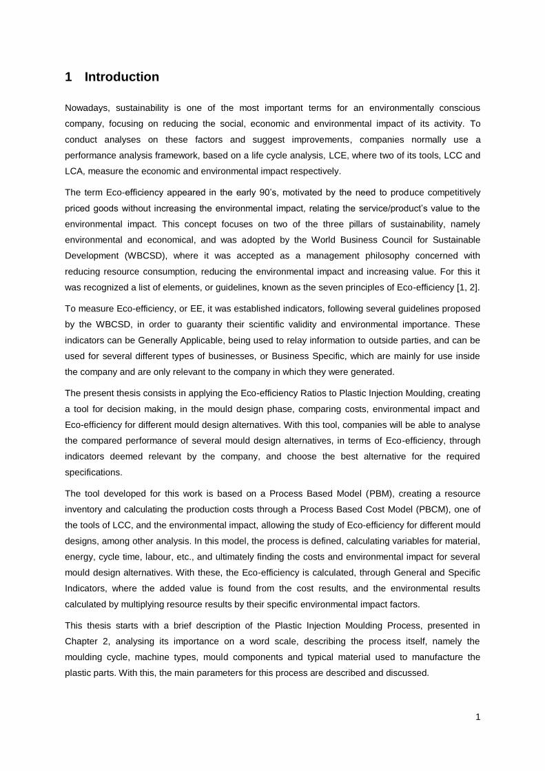
1 Introduction
Nowadays, sustainability is one of the most important terms for an environmentally conscious
company, focusing on reducing the social, economic and environmental impact of its activity. To
conduct analyses on these factors and suggest improvements, companies normally use a
performance analysis framework, based on a life cycle analysis, LCE, where two of its tools, LCC and
LCA, measure the economic and environmental impact respectively.
The term Eco-efficiency appeared in the early 90’s, motivated by the need to produce competitively
priced goods without increasing the environmental impact, relating the service/product’s value to the
environmental impact. This concept focuses on two of the three pillars of sustainability, namely
environmental and economical, and was adopted by the World Business Council for Sustainable
Development (WBCSD), where it was accepted as a management philosophy concerned with
reducing resource consumption, reducing the environmental impact and increasing value. For this it
was recognized a list of elements, or guidelines, known as the seven principles of Eco-efficiency [1, 2].
To measure Eco-efficiency, or EE, it was established indicators, following several guidelines proposed
by the WBCSD, in order to guaranty their scientific validity and environmental importance. These
indicators can be Generally Applicable, being used to relay information to outside parties, and can be
used for several different types of businesses, or Business Specific, which are mainly for use inside
the company and are only relevant to the company in which they were generated.
The present thesis consists in applying the Eco-efficiency Ratios to Plastic Injection Moulding, creating
a tool for decision making, in the mould design phase, comparing costs, environmental impact and
Eco-efficiency for different mould design alternatives. With this tool, companies will be able to analyse
the compared performance of several mould design alternatives, in terms of Eco-efficiency, through
indicators deemed relevant by the company, and choose the best alternative for the required
specifications.
The tool developed for this work is based on a Process Based Model (PBM), creating a resource
inventory and calculating the production costs through a Process Based Cost Model (PBCM), one of
the tools of LCC, and the environmental impact, allowing the study of Eco-efficiency for different mould
designs, among other analysis. In this model, the process is defined, calculating variables for material,
energy, cycle time, labour, etc., and ultimately finding the costs and environmental impact for several
mould design alternatives. With these, the Eco-efficiency is calculated, through General and Specific
Indicators, where the added value is found from the cost results, and the environmental results
calculated by multiplying resource results by their specific environmental impact factors.
This thesis starts with a brief description of the Plastic Injection Moulding Process, presented in
Chapter 2, analysing its importance on a word scale, describing the process itself, namely the
moulding cycle, machine types, mould components and typical material used to manufacture the
plastic parts. With this, the main parameters for this process are described and discussed.

2
In Chapter 3 a brief history of sustainability is presented, along with the life cycle performance analysis
methodologies, followed by Eco-efficiency, introducing its principles and indicators.
The methodology followed to create the model for this work is presented in Chapter 4, and the model
developed is presented in Chapter 5, explaining a typical PBCM and demonstrating how each cost,
and environmental impact, was calculated. Still in this chapter, the model is validated through the
costs, using a case study presented in a previous work.
The results are presented and analysed in Chapter 6, for several mould design alternatives, with
different number of cavities, feeding system and machine type. This chapter illustrates the ultimate
goal of this work, where different mould design alternatives are compared in terms of their Eco-
efficiency performance, for both General and Specific Indicators, and the best alternative is
determined.
The suggested approach for Eco-efficiency comparison with this model is illustrated in Chapter 7,
describing which variables the user must define and the results and analysis the model is capable of
providing, along with a sensitivity analysis of cost and environmental impact to production volume and
part thickness.
Finally, the conclusions are presented in Chapter 8 and future work is described in Chapter 9.

3
2 Plastic Injection Moulding
Plastics have become increasingly important, being used to replace metals and other materials in
several engineering and industrial applications [3].
The most common manufacturing process for plastics is the injection moulding process encompassing
the melting, injection, packing, cooling and ejection phases, with possible quality control as an
additional phase performed by workers. Understanding the process is essential to produce faster and
cheaper products with high quality and minimize defects such as warpage, welding lines, etc., reduce
energy consumption and increase the product’s life time [4, 5].
In this chapter, the injection moulding process is discussed, presenting a brief history, describing the
moulding cycle, injection machine, mould components, materials and, finally, the main variables of this
process and how they can affect its performance.
2.1 Technology on a global scale
Plastic injection moulding is used for mass production of thermoplastic and thermosetting materials
through moulds, with a variety of shapes and sizes, with the application of heat and pressure.
This technique was first developed in the late 1800’s, used for simple objects such as buttons,
revolutionizing the plastics industry in 1946 when the first screw injection moulding machine was
designed, still being used to this day [6]. Since 1995, the number of polymers available for injection
moulding has increased significantly, approximately 750 per year, having started with 18.000,
including blends of previous materials, allowing for the selection of the best set of properties for each
product. Now, this process consumes approximately 32% of all plastics worldwide, only second to the
extrusion process which consumes 36% [7, 8].
In terms of mould production, Portugal is the world’s eighth largest mould-making country, centred in
Marinha Grande, exporting nearly 90% of its production. The industry invests a significant percentage
of total sales, approximately 10%, for new development and innovations allowing significant advances
in design and production capabilities [9].
Since the injection moulding process is one of the most versatile production processes, the
applications have varied, as a result of extremely different properties between polymers, necessities
and overall quality, with plastic parts replacing several products [10]. These developments include the
plastic spring, which was not possible until recently, mechanical parts, including gears and some
musical instruments or parts of them, among other new applications. Yet, this process is useful for
producing high volume rates, in the thousands or millions of parts, still being cost-effective, with
products varying from the micro-scale to the macro-scale [11].

4
2.2 Process description
Although injection moulding is a manufacturing technology to process both sets of plastics,
thermoplastics have a higher demand, when compared to thermosets, due to certain characteristics,
such as recyclability and additional ease to soften and flow when heated [12].
In terms of equipment, the machine to process thermoplastics uses a screw-type plunger to force the
molten material, in the form of a viscous liquid, into a mould cavity, at high pressure and temperature
where the material solidifies and is ejected [12]. This is called the moulding cycle.
2.2.1 Moulding cycle
The main phases of the injection moulding process are injection, packing, cooling, and part ejection,
where the closing of the mould can be included in the injection phase. This sequence of events is
called the injection moulding cycle [13].
As illustrated in Figure 2.1, the cycle starts when the mould closes, followed by the plastic injection
into the mould cavity and ends when the mould opens and the final part is ejected.
Figure 2.1 – Typical Injection Moulding Cycle [14]
The raw material is used in the form of plastic pellets or powder, which are fed into a hopper and from
there to a heated cylinder to soften the material into a viscous fluid. When a certain temperature is
reached, the screw, located in the cylinder, starts rotating, moving the material forward and
additionally heating the polymer due to the friction against the walls. When all material is in the mould
cavity, the screw maintains pressure, which is predetermined, during a short period of time allowing
the material to solidify in the mould and not recede to the cylinder. In the mould is located a cooling
system, which can be more or less complex depending on the size and complexity of the mould and
the final part. The cooling system is composed of channels where cooling liquid flows, usually water or
oil, allowing to cool the mould. When the choice of cooling fluid is made, a careful evaluation and
design of all cooling parameters is needed including diameter and location of channels and cooling
time [15].
When a certain mould temperature is reached, controlled by the time the material remains in the
mould cavity and the fluid temperature and design of the cooling system, the final part is ejected from
the mould through a set of ejector pins, located in the mould, and left to cool at room temperature. The

5
mould is then closed and the cycle is repeated [15]. This cycle time is one of the most important
parameters in injection moulding as the rate of production and the quality of the parts is dependent on
it [13].
According to Figure 2.1, it is possible to affirm that the cooling phase encompasses most of the cycle
time, and can take up to 80% of the cycle time, depending on the polymer and quality of the final part,
whereas the injection and packing phases are relatively quick and cannot be reduced much further. As
such, it is possible to deduce that to reduce cost and increase production rate, maintaining all other
aspects of production, cooling time reduction is necessary. However, this step needs to be performed
carefully as decreasing the time excessively can cause shrinkage and warpage, as well as defects
due to the ejection force applied to remove the part, damaging the final part beyond repair [13].
2.2.2 Injection Machine
The most common machine is composed of two main units, the injection unit and the clamping unit.
The first guarantees the material feed and pressure and the second the mould opening/closing during
each injection cycle, as well as the clamping pressure to ensure the mould remains closed during
injection. These units are illustrated in Figure 2.2.
Figure 2.2 - Injection Moulding Machine [15]
Injection moulding machines have different configurations and many different components, including a
horizontal and vertical configuration where the injection is performed in a horizontal or vertical position,
respectively. Regardless of their differences, each machine needs a power source and mould
assembly, in addition to the main units, as seen in Figure 2.2 [16].
In terms of operating systems, injection moulding machines can be divided in three main groups:
hydraulic, electrical and hybrid. With an all-oil hydraulic machine, the power required to turn the screw
and melt the material, inject and hold pressure, etc. is guaranteed by oil pressure. For this, a central
power source is used to supply energy to all functions of the machine through the use of valves,
pumps, among others [17].
Electrical moulding machines are available worldwide but still less used than their hydraulic
counterparts, despite its many advantages which include quick setup and start-up, elimination of oil,
high moulding quality and productivity. As a result of oil elimination, with addition of low noise and

6
compact size, the environmental impact is reduced making this electrical machine indicated for highly
populated areas [17].
However, hydraulic machines will, for the foreseeable future, continue to be strong contenders in the
market. This is a result of the cost advantages, providing better value, and a secure market in the
high-tonnage applications.
Summing, it is possible to affirm that hydraulic machines waste energy converting electricity to
mechanical force whereas the electrical injection moulding machine can save 50% to 90% of power
and reduce the environmental impact due to its innate properties. [17]. Hybrid machines, which are a
combination of electrical and hydraulic, have advantages of both power systems. However, these
machines are only now being applied, depending on the balance between the necessary
characteristics and the cost, since for a high tonnage, for example, hydraulic components are needed,
which induce a lower cost but an increase environmental impact [17]. Thus a detailed analysis is
needed for the use of these machines.
Typically, injection moulding machines are characterized by the clamping force, meaning the force
applied to the mould in order to maintain the mould closed during the injection phase, which is
determined by the projected area of the parts in the mould and the pressure with which the material is
injected. With this it is possible to conclude that larger parts, with higher projected areas, or higher
injection pressures, require greater clamping force [16]. However, the type of machine, hydraulic or
electric, must be considered as the latter allow for a lower clamping force, thus are not suitable for all
product alternatives.
Finally, in order to guarantee the complete fill of the mould cavity and the quality of the final part, the
right machine needs to be chosen in terms of: 1) shot capacity, which is the amount of material
injected into the mould; 2) clamp stroke, the distance each mould part needs to travel in order to
securely close the mould, which needs to be large enough to allow the part to be ejected, 3) minimum
mould thickness and 4) the size of the plate onto which the mould halves are mounted, in order to
guarantee the correct size mould [16].
2.2.3 Mould
Mould design is a complex and lengthy subject due to all parameters and considerations to be made
by designers, meaning it requires experience and time for improvement.
Moulds can be of single or multiple cavities, where each cavity can be identical or form different
components with each injection cycle. Furthermore, both types of moulds can include inserts, usually
metallic, with which the plastic will bond and form the final part [18].
Moulds are generally made of tool steel, which presents a higher manufacturing cost but also a higher
resistance, hence a higher life time, meaning the initial investment will be eventually returned,
depending on the production volume. In some cases moulds are made of aluminium which costs less
initially, but has a reduced life, when compared to tool steel moulds, being suitable for lower

7
production volumes. The latter are also not adequate for parts with narrow dimensional tolerances due
to the damage and deformation that may occur during the injection, as a result of high pressure
values, or caused by the clamping cycles applied by the machine [19, 18].
The typical injection mould consists of two parts: core and cavity, forming the part cavity. The plastic
material enters through a sprue into the mould cavity, pushed by the screw in the injection unit’s
cylinder, remaining in the mould cavity, when solidified, until a set of ejector pins is activated [16].
For the material to flow from the sprue into the mould cavity, several channels, called runners, are
integrated into the mould design [16]. For injection moulding there are two common runners
designated by the temperature of the melt when injected: cold runners and hot runners. With cold
runners the plastic is injected through the sprue into the mould, solidifying in the mould cavities and
the runners, which are ejected with the part. On the other hand, hot runners are used to inject the
polymer into the mould cavities, and only the part is ejected, maintaining the remaining material in the
runners to be used in the next cycle. With this alternative there can be one or several injection points,
chosen to facilitate the process or improve the part’s quality. This type of feeding system is well suited
for polymers with thermal variation sensitivities and can include mechanisms for removing any marks
of injection [17].
Comparing cold and hot runners, the first have a lower cost and accommodate a wide variety of
polymers but produce waste, even if the removed runners can be recycled, and the latter have
potential for faster cycle times and no waste production. However, these are more expensive and
require higher maintenance contributing to an increase in downtime [17].
Another set of channels are included in the mould, the cooling channels, to cool the molten plastic,
allowing the cooling fluid to flow through the mould walls, as previously mentioned.
Finally, air vents are typically included in the mould design, in order for the air trapped in the mould,
resulting from the injection moulding process, to escape avoiding defects in the final part or increased
pressure inside the mould.
An example of a mould is illustrated in Figure 2.3.
Figure 2.3 – Mould Example [16]
8
2.2.4 Materials for injection moulding
For injection moulding there is a wide variety of possible materials to be considered, from
thermoplastics to thermosetting, depending on their characteristics and the intended use of the final
part, as well as the necessary quality required by the customer. These plastics can be used singularly,
or as a combination of multiple materials, in order to improve certain characteristics with the possible
addition of colorants [16]. Still, one must always take into consideration the cost of raw material, for its
influence in the final part’s cost, and type of material due to its ease of processing
Among the world of plastics and combinations to choose from, there are a few which are most
commonly used either for the ease of processing, cost or final requirements. In Table 2.1 is described
some of the characteristics of these common materials, as well as examples of their applications.
Table 2.1 – Most Common Materials in Injection Moulding Process [16, 20]
Material Name Abbreviation Description Application
Acrylonitrile-Butadine-
Styrene ABS
Strong, flexible, chemical
resistance, low mould
shrinkage
Automotive industry, boxes,
toys
Polyamide (Nylon) PA
High strength, fatigue
resistance, chemical
resistance, low friction
Bearings, gears, wheels
Polycarbonate PC Very tough, temperature
resistance, dimensional stability
Automotive industry,
containers, light covers,
safety helmets
Polyethylene
Terephthalate PET
Rigid, heat resistance,
chemical resistance
Automotive industry, electrical
components, valves
Polypropylene PP
Lightweight, heat resistance,
high chemical resistance,
scratch resistance
Automotive industry, bottles,
caps, crates, handles
Polystyrene PS Brittle, transparent Cosmetics packaging, pens
2.3 Process analysis – variables and their influence in process performance
Injection moulding is a complex manufacturing process in the sense that it offers the possibility to
produce products with complex geometry, where identical or different parts can be produced in the
same cycle, with dimensions raging from the macro to the micro-scale, multicolour products or multi-
components, referring to the addition of inserts, and production of hollow parts [21, 22, 23]. As such, it
is to be expected an array of multiple variables, important in one or several parameters. From the
available bibliography it is concluded that type of machine, mainly in terms of energy, material type
and cost and cycle time are considered the most influential parameters in the injection moulding

9
process, but it was not conclusive how the different variables can influence the process for each of
these parameters.
As most studies performed to date are mainly concerned with energy and material consumption, it is
important to start by understanding how different parameters and variables can influence these
aspects.
Recently, there has been an increasing concern regarding energy consumption in the plastic injection
moulding process, resulting of the fact that higher consumptions suggest higher costs and
environmental impacts, considering 1 kWh of energy consumed will produce approximately 0,43 kg of
CO2. As such, energy saving should not only be considered during the injection phase, studying the
injection machine alone, but during the phases of mould and part design and material selection [22,
23, 21]. However, as most studies indicate that the main energy consumption is due to the injection
machine, is it worth to understand how this energy is consumed.
In Figure 2.4 is illustrated the distribution of energy consumption regarding all the basic and additional
equipment used in this process, where the peripheral equipment consists of all the dryers and cooling
systems.
Figure 2.4 - Energy Consumption in Injection Machine [23]
With the figure it is possible to verify that all basic components, meaning the components related to
melting, filling and cooling stages, to an injection moulding machine are where most of the energy is
consumed. Hence, the right machine type and specifications are paramount to reduce energy
consumption. For this, studies have shown that electric machines have lower energy consumption
when compared to other types, mainly as a result of no additional energy being used during the
cooling phase, and a reduced cycle time resulting in a faster manufacturing process, in spite of having
a higher initial cost then the other two possibilities [21, 22, 23].
Although this type of machine contributes less with an environmental impact, studies have been
performed in order to improve efficiency in all machines. Additional improvements, related to energy
consumption, can be made adding insulation to the cylinder to minimize heat transfer through
convection and a proper selection of machine dimensions and power capacity [21, 22, 23].
1%
17%
33% 32%
15%
2% Robot
Heating of plasticizingunitMould temperatureregulationInjection mouldingmachine drivePeripheral equipment
Injection mouldingmachine control

10
The decrease of energy consumption, in the part design phase, starts with the knowledge and proper
selection of materials. For example, for amorphous materials, such as polystyrene or polycarbonate,
the main source of heat is conductive, being transferred from the cylinder wall to the material, whereas
semi-crystalline materials, such as polyamide, require an increase of cylinder temperature or screw
pressure in order to achieve the correct melt flow values. Some thermoplastic materials, such as PET,
ABS and PC, have natural moisture that needs to be reduced, through the use of dryers, to guarantee
the highest possible quality in the final product as well as increase production efficiency. This drying
cycle is applied to combat the defects caused by steam in the final part, machine or mould, if moisture
is not removed when the granules are processed [21, 22, 23].
When considering the mould itself, the selection of appropriate material and the correct design of
cooling channels will contribute to temperature regulation of the mould cavity, thus influencing the
cooling time. However, caution must be exercised when shortening this time as the minimum cooling
time must be respected, which is influenced by the type of material. As such, the mould cavity material
influences the process cycle time which, in turn, is influenced by the cavity wall temperature, contact
temperature and cooling fluid temperature. When, for example, a required temperature is defined, if a
material with lower thermal conductivity is used, the overall cycle time is shorter due to the fact that it
is possible to achieve the required temperature with lower temperature of the melted polymer and thus
decreasing energy consumption [23]. As such, is possible to conclude that material’s thermal
properties are also influential when discussing cycle times and energy consumption.
The frictional heat, or energy, caused by the friction between the plastic pellets and the cylinder walls,
is determined by the velocity at which the material is fed into the cylinder and the injection speed. The
latter is influenced by the moulded parts wall thickness, flow length and, in no small way, the type of
plastic to be processed. With the growing development of materials, or mixture of existing materials,
production is improved due to the all-around better properties, meaning shorter cycle times resulting in
the decrease of energy and material consumption [21, 22, 23].
Until recently, material selection was performed almost exclusively considering cost of raw material,
disregarding the costs of processing the chosen material. However, and as explained previously, for
the plastic injection moulding process, the productivity is mainly determined by the cooling time which
highly influences the cycle time, where the most influential parameter in the cooling time is wall
thickness [24]. As such, the use of materials which enable the decrease of wall thickness will result in
shorter cooling times and, through this, decrease the overall cycle time, thus contributing to energy
savings and a possible decrease in processing costs.
In Figure 2.5 is possible to observe the resulting decrease of wall thickness due to the appropriate
material selection.

11
Figure 2.5 - Comparison of moulded parts wall thickness with different materials [23]
Still, when choosing better materials the cost must be an important factor as a state of the art material
will undoubtedly have a higher cost, but might not improve significantly the energy and material
consumption. Such materials are also, sometimes, difficult to work with or workers have no experience
meaning also an increase in labour cost. Summing, considering the set of requirements, it is possible
to choose the adequate material, or materials, in the moulded part development phase, in order to
increase energy and material savings [21, 22, 23].
When considering the mould itself, the selection of appropriate material and the correct design of
cooling channels will contribute to temperature regulation of the mould cavity, thus influencing the
cooling time. However, caution must be exercised when shortening this time as the minimum cooling
time must be respected, which is influenced by the type of material and the part geometry. As such,
the mould cavity material influences the process cycle time which, in turn, is influenced by the cavity
wall temperature, contact temperature and cooling fluid temperature.
With all these considerations it is possible to conclude that there are several parameters such as: type
of material, wall thickness, cooling fluid temperature, flow speed, temperature of melt, etc. that
influence the quality of the final part, as well as the energy consumption and material waste, when
considering that an improper choice of parameters will cause defects in the final part that might not be
acceptable, taking into account all the ancillary processes and not just the injection moulding process
itself. Due to the large scale of this industry, any increase in efficiency resulting of well thought out and
well-designed components will lead the large saving both economic and for the environment [25].
From these studies it is possible to verify that the main focus has been material and energy
consumption, leading to believe that these are the most important parameters in plastic injection
moulding, and cycle time, which is established as the most influential parameter in this process.
However, these are influenced by several variables, as demonstrated, including part and mould design
and type of machine. As such, it is important to understand how different aspects of part, mould and
machine will affect the cycle time and, ultimately, the material and energy consumption, translating to
both economic and environmental results. Still, these are not the only variables and parameters to this
process, hence a more detailed analysis of other aspects of part, mould and machine choice must be
performed in order to guarantee an accurate result.

12
3 Performance evaluation in a Life Cycle Perspective
Nowadays, the growing population rate strongly contributes to the shortage of natural resources and
increase of waste accumulation leading to severe problems, mainly related to the environment. The
present-day situation has put a high demand on world businesses to take responsibility for the growing
ecological problems such as CO2 emissions, waste management and deforestation, among others
[26], with “communication as a key to achieving sustainability” [27].
This chapter contains a brief historical note on sustainability and how it can affect the world, followed
by the principle method for performance analysis in a life cycle perspective, Life Cycle Engineering
(LCE), for sustainable production, and two of its tools, namely Life Cycle Assessment (LCA) and Life
Cycle Cost (LCC). Focusing especially in terms of Eco-efficiency, which encompasses two of the three
pillars of sustainability, it is described its philosophy and principles, taking special focus on how to
measure Eco-efficiency. Finally, is discussed the importance of these aspects in several industry
applications, focusing on the plastic injection moulding sector.
3.1 Historical evolution of sustainability
“Sustainable development has become a “buzzword” of both academic and the business world” [26]
as the demand for sustainable products is increasing, companies, and suppliers, will have a
competitive edge if they adjust to more environmentally friendly and cost effective production [27]. As
such, in order to predict the future trends and problems that will appear, it is important to understand
the history and evolution of the concept of sustainability [28].
The first international conference, Conference on the Human Environment, devoted exclusively to the
environment, took place in 1972 in Stockholm, Sweden, where experts established the links between
environment and development stating that: “Although in individual instances there were conflicts
between environment and economic priorities, they were intrinsically two sides of the same coin” [28].
From then on, several conferences were made devoted to the subject, where one of the most
important was the Kyoto Conference on Climate Change, in 1997, where the main focus was to
reduce greenhouse gas emissions, creating the framework for the Kyoto Protocol with specifics to be
developed over later years. However, it only outlined the basic features for compliance but it did not
explain the rules of how they would operate. Even with this setback, 84 countries signed the Protocol
indicating their intent to rectify it [28].
The World Summit of Sustainable Development took place in 2002 in Johannesburg, South Africa,
resulting in the Johannesburg Declaration of Sustainable Development as well as the Plan of
Implementation on the World Summit on Sustainable Development. Same year, the Global Reporting
Initiative (GRI) introduced the second generation of guidelines on reporting of economic, social and
environmental initiatives [26].

13
From these conferences and gatherings it was established that the three aspects of sustainable
development, also called “the triple bottom line” or “the 3P’s”, are: planet, people and profit. Economic
sustainability focuses on securing economic viability in short and log terms whereas social
sustainability is achieved when the population feel they can have a fair share of wealth, safety and
influence. Environmental sustainability “seeks to improve human welfare by protecting the sources of
raw material used for human needs and ensuring the level of human waste is not exceeded in order to
prevent any harm caused to human beings” [29]. These three pillars of sustainability are illustrated in
Figure 3.1.
Figure 3.1 - Three main aspects of Sustainability [26]
As such, it is possible to conclude that sustainable development is dependent on both consumers and
producers. This can clearly be deduced from the definition of Sustainable Production given by the
Lowell Centre for Sustainable Production as “the creation of goods and services using process and
systems which are non-polluting, conserving of energy and natural resources, economically viable,
safe and healthful for employees, communities, consumers and socially and creatively rewarding for
all working people” [29]. Another definition supporting this statement is of Sustainable Consumption,
as “the use of goods and services that respond to basic needs and bring a better quality of life, while
minimizing the use of natural resources, toxic materials and emissions of waste and pollutants over
the life cycle, so as not to jeopardize the needs of future generations” [29]. Knowing this, it is possible
to conclude that the actions of individuals, as well as companies, will have a profound effect on
sustainability.
Until recently the concept of sustainable production was considered extremely expensive to be put in
practice by major corporations and governments [28]. However, as ideas of sustainable development
are becoming more mainstream and taken more seriously, the majority of companies are adopting
them as leading principles for their operations [26].

14
3.2 Methodologies and approaches for performance analysis in a life cycle
perspective
Along the last two decades sustainability and social responsibility are two of the main ideas when
thinking of business strategies [30].
“Within sustainable product development approaches, life cycle approaches are nowadays established
as the most apt to capture the full impacts of design decision” [31]. To evaluate the design impacts on
the environment and production costs, several studies use the Life Cycle Engineering (LCE) method
[32], namely Life Cycle Assessment (LCA) method to assess a single environmental indicator, while
other methods focus on a particular environmental factor, usually greenhouse gas emissions,
resources and energy efficiency or environmental targets such as recycling or hazardous materials,
and Life Cycle Cost (LCC) to evaluate the economic factor in the design phase. Still, life cycle analysis
is common to all approaches and is extremely important when studying various sectors of the industry
[31].
3.2.1 Life Cycle Engineering (LCE)
With the necessity of creating better and cheaper products, Design-for-X has been increasingly and
successfully implemented. This strategy drives the company, or design team, to create products and
services for a specific target or to minimize impact. However, this method restricts analysis for it only
focuses on one aspect as, for example, the objective of design for cost is to minimize the production
costs, design for environment is used to lower environmental impact focusing on product material and
design for assembly aims to minimize the effort of the assembly task. As such, this approach does not
consider multiple design objectives and does not take into account the overall impact of a design
decision. For this is used the Design for Life Cycle, or Life Cycle Engineering (LCE), which considers
all phases of a products life cycle in the early design phase [32].
The motivation to perform an LCE study is to minimize the environmental impact and costs associated
with production having in mind all regulations and standards [30], where there are three main
considerations to be made during the decision making process: Economic, by means of the Life Cycle
Cost, Environmental, considered in the Life Cycle Assessment, and Technical, to guarantee the
product performs as requested [33].
This method allows to: (i) communicate the connection between environmental impacts and
engineering requirements, (ii) assess the environmental implications of applied alternatives and (iii)
identify opportunities for improvement within the life cycle.
Due to the fact that LCE has no precise definition, Jeswiet has presented a widely known image,
Figure 3.2, which defines LCE through its keywords.

15
Figure 3.2 - Keywords of LCE [32]
Although LCE is to be developed during the initial design phase, this involves a large effort as a large
number of materials and design options are available. To reduce this there are several factors to limit
the design alternatives and thus use LCE analysis only on the most promising. As only a few
alternatives will be considered this can be considered a drawback when compared to the Design-for-X
framework, if not for the way the three main indicators are used. For the economic aspect is used the
LCC methodology for cost estimation integrating design for cost, design for maintainability, etc. For the
environmental indicators is used the LCA approach including design for environment, design for
recycling, etc. The technical aspects are evaluated, for example, in the design for reliability or design
for use [32].
Summing, LCE studies the performance, cost and environmental impacts, translating to engineering
requirements, and allows to compare alternatives on a sustainability and life cycle perspectives though
a ternary diagram built according to the results of each analysis [34, 35].
3.2.2 Life Cycle Assessment (LCA)
According to Jim Java, one of the founding fathers of LCA, “life cycle assessment has become a
recognized instrument to assess the ecological burdens and human health impacts connected with the
complete life cycle of products, processes and activities, enabling the practitioner to model the entire
system from which products are derived or in which processes and activities operate” [34]. As such,
the LCA can be defined as a tool to evaluate environmental impacts and resources consumed
throughout the products life cycle from raw material acquisition to waste management [32].
In the ‘80s, the life cycle assessment was developed as a tool to better understand the risks and
opportunities as well as the environmental impacts of production systems, avoiding the shift of a
product’s environmental problem to other life cycle phases or other parts of the production system
[34]. Beginning in 1993, the International Organization for Standardization (ISO), together with a group
of Society of Environmental Toxicology and Chemistry (SETAC) experts, recommended the
standardization of the LCA method and by 1997 the ISO 14040 standard for Life Cycle Assessment –
Principles and Framework was complete [31], defining LCA as the “compilation and evaluation of the

16
inputs, outputs and the potential environmental impacts of a product system throughout its life cycle”
[36].
Still, this method is time consuming and expensive where designers have to make decisions,
especially when studying complex systems, and results have to be interpreted and weighed. To
complement this analysis, environmental performance indicators are integrated, known as the Key
Environmental Performance Indicators (KEPI) and the Eco-efficiency Indicators (EEI), which have
proven to be effective in the last step of an LCA. With this addition, the methodology becomes simpler,
in the sense that the results can easily be interpreted and compared, but more complex considering
the inclusion of several steps to the LCA framework. As such, the approach is built in the following
steps: (i) scope and boundary definition, (ii) life cycle inventory, (iii) life cycle impact assessment, (iv)
KEPI, (v) Product/service value and (vi) EEI [31].
In Figure 3.3, is illustrated the previous steps and their relations, where the EEI are EEIgiven by the
ratio between Product/Service Value and the results of the LCIA.
Figure 3.3 - Revised LCA framework [31]
LCA analysis in the design phase is often excluded since it is usually assumed not to contribute
significantly to environmental factors. Still, decisions in design strongly influence the impacts in other
life cycle phases since the product’s design influences its behaviour in subsequent phases [37].
3.2.3 Life Cycle Cost Analysis (LCC)
Life cycle costing (LCC) appeared in the 60’s, used by the US government as a means for cost
optimization when acquiring large equipment goods [38]. The US Department of Defence published
guidebooks, in the early 70’s and ever since many theories on LCC have taken place [39]. However,
the importance of estimating and controlling costs during the design phase, with the objective of
limiting its production costs, is of extreme importance for developing a cost effective product [30].

17
This is not a standard analysis and, according to literature, there are a vast number of approaches
varying on the form and scope, where LCC evaluates the product’s life cycle in terms of costs,
considering all costs, including costs that are not normally expressed in the product market price, such
as costs during usage and disposal [32], or only the main costs and benefits associated with each
alternative activity or project over its life cycle [39]
Meanwhile, guidelines for this approach are being developed by the Society of Environmental
Toxicology and Chemistry (SETAC) in order to ensure identical system boundaries, meaning the life
cycle cost methodology is to be applied from cradle-to-grave and not during the marketing life cycle
(from product development to end of market life) [34]. According to the principles of Greene and Shaw
(1990), the LCC analysis is guided by the steps presented in Figure 3.4.
Figure 3.4 - Life Cycle Cost Analysis Procedure [38]
One of the tools of Life Cycle Cost analysis is called Process-Based Cost Modelling which compares
design alternatives by correlating cost with design changes, allowing to perform sensitivity analysis to
process and design parameters, in each process of the life cycle [32]. An example is illustrated in
Figure 3.5, where process modelling establishes the relation between the production process and its
parameters, operation modelling defines all necessary resources and, finally, the financial model
delivers all final costs.
Figure 3.5 - Process-Based Cost Modelling [30]
Despite the apparent similarities, LCC and LCA have different backgrounds and differences in
methodology due to the fact that each approach is used to answer different questions, respectively
economic and environmental questions, as mentioned before. Life cycle cost analysis compares cost-
effectiveness of alternative investments or decisions in an economic perspective, studied throughout
the economic lifetime of the investment, which can be shorter than the “use-phase” of an LCA, and is
to be considered during the earliest stages of development, as opposed to the LCA which is not
normally considered at such early stages. Still, the consequences of using LCA without LCC are: (i)
limited influence and relevance in decision making, (ii) ineffective link between environmental and

18
economic impacts, also compromising the ability to search for cost-effective environmental
improvements and (iii) possibility of missing crucial economic related environmental consequences. Its
limitations include the necessity of a large amount of data, which can lead to substantial setbacks
when procedures are not followed [40].
3.3 Eco-efficiency
3.3.1 Philosophy and Principles
The term Eco-efficiency first appeared in 1990 in Switzerland, proposed by Schaltergger and Sturm,
and was adopted by the World Business Council for Sustainable Development (WBCSD) in 1991. This
concept was mainly focused on issues within companies, later extending to help assess policy
strategies and their macroeconomic outcome, as a result of an increasing pressure on companies and
governments to develop sustainable alternatives and products, Eco-efficiency has emerged as a
useful tool relating value of a product with its environmental impact [1].
“Companies adopting eco-efficiency are more often among the leaders in their sector. As
their success inevitably and constantly provokes many others to follow, eco-efficiency will
finally grow into the mainstream” – Frank W. Bosshardt, Policy Adviser ANOVA Holding
AG, Founder of the WBCSD Eco-efficiency Program [41].
According to the WBCSD, Eco-efficiency is “a management philosophy that encourages business to
search for environmental improvements that yield parallel economic benefits, focusing on business
opportunities and allowing companies to become more environmentally responsible and profitable,
and is a key business contribution to sustainable societies” [31], concerned with three objectives: (i)
reducing the consumption of resources by minimizing the use of energy and materials, enhancing
recyclability, etc. (ii) reducing the impact on nature by minimizing air emissions, waste disposal, etc.
and (iii) increasing product /service value, meaning the possibility for the customer to receive the same
functional need with fewer materials and less resources [41].
As defined by the WBCSD, “Eco-efficiency is achieved by the delivery of competitively priced goods
and services that satisfy human needs and bring quality of life, while progressively reducing ecological
impacts and resource intensity throughout the life cycle to a level at least in line with the Earth’s
estimated carrying capacity” [2]. Summing, Eco-efficiency is concerned with creating more value and
less impact, being measured by the ratio between economic growth and environmental impacts,
where the highest indicator is achieved when a product value is increased and the environmental
impacts decreased. The economic value can be quantified as the amount of products, net sales or
added value, among others, and the environmental performance by the amount of energy, materials or
resource consumption [31].
Having this in mind, the WBCSD established seven elements that can be addressed for Eco-efficiency
improvement, known as the Eco-efficiency principles [1]:
1) Reduce material intensity

19
2) Reduce energy intensity
3) Reduce dispersion of toxic substances
4) Enhance recyclability
5) Maximize the use of renewable resources
6) Extend product durability
7) Increase service intensity
The concept of Eco-efficiency has evolved from preventing pollution in manufacturing to a driver of
innovation and competitiveness between companies and countries. However, it will never work as an
add-on to a company due to the fact that it is not sufficient by itself, as it only integrates the economics
and ecology elements of sustainable development, but should always be an integral part of business
strategy [2].
Eco-efficiency requires skills and capabilities such as understanding definitions and issues, analysing
stakeholder’s perspectives to implementing a life cycle assessment with measuring and evaluating
impact. Although there are several case studies on the subject, it is still necessary to draw on the
experience of experts to implement and achieve the goals proposed. However, this is a philosophy still
in progress, as it should be to accommodate the changes in necessities worldwide [2].
This is a concept widely criticized for “restricting industry growth and for limiting creativity and
productiveness” [2] and for not achieving the goals of sustainable development. However, it seeks
more efficient growth and in so doing calls for “creativity and productiveness” on the part humankind
and it is intended to give a helpful tool for companies to “better their business while playing their part in
the environmental side of sustainable development” [2]. As such, the criticism of the term Eco-
efficiency often comes from lack of understanding.
The objective now, in terms of the Eco-efficiency philosophy is to move from crisis-avoidance
mentality to implementing as a part of the foundation of every project [2].
3.3.2 Performance Measure and Indicators
Eco-efficiency indicators rose from the need to measure and quantify Eco-efficiency, and are used
worldwide as a management tool to assess a company’s progress on a certain requirement. As such,
an indicator relays important qualitative and quantitative information for decision making and can be
defined as a parameter or a reference value of a parameter [42].
The WBCSD suggests the indicators should [43]:
(i) “Be relevant and meaningful with respect to protecting the environment and human health
and/or improving the quality of life”
(ii) “Inform decision making to improve the performance of the organization”
(iii) “Recognize the inherent diversity of business”
(iv) “Support benchmarking and monitoring over time”
(v) “Be clearly defined, measurable, transparent and verifiable”

20
(vi) “Be understandable and meaningful to identified stakeholders”
(vii) “Be based on an overall evaluation of a company’s operations, products and services,
especially focusing on all those areas that are of direct management control” and
(viii) “Recognize relevant and meaningful issues related to upstream (e.g. suppliers) and
downstream (e.g. product use) aspects of a company’s activities”.
The ultimate goal of these eight principles is to ensure the indicators are scientifically supported and
environmentally relevant, relating to issues where there is a clear need for improvement, accurate and
useful for all businesses, considering the indicators for different products or processes must be
defined in the same way so that comparisons are made regarding the same units, and must be
designed to minimize the influence of extraneous factors in order to avoid “false” changes in Eco-
efficiency, allowing to improve the performance of businesses and monitoring that performance with
transparent and verifiable measures, clearly defined by estimation methodologies, and limitations with
individual indicators clearly understood. These indicators must also be meaningful to both internal and
external members of a company, such as business managers and stakeholders respectively, mainly
focusing on all areas of a business’s operations, products or services but also recognizing the
relevance of issues upstream and downstream of a company’s activities [43].
The Eco-efficiency indicators can be classified as Generally Applicable indicators, used by any
business, relating to a global environmental concern or business value, with measuring methods
accepted globally, using available metrics such as EI’99 or ReCiPe for environmental impact
measurement, or Business-Specific indicators which are defined from one business, or sector, to
another, not being necessarily less important than the first group. For the latter, the WBCSD
recommends the use of the ISO 14031 standard as a guide for the selection of relevant indicators [43,
44].
“A company’s Eco-efficiency profile will include both types of indicators” [2] where the WBCSD
recommends the use of a limited number of Generally Applicable Indicators and a set of Business
Specific Indicators in order to keep the company’s Eco-efficiency profile as clear as possible [43].
An important sub-group of Business Specific Indicators are the KEPI (Key Environmental Performance
Indicators), which are useful to demonstrate the impacts in a measurable level, meaning in relation to
the functional unit defined by the company, so the results are presented in the form of a metric, in
accordance to the objectives of the company [44, 31]. The purpose of this functional unit is to provide
a reference to which results with different units can be related. However, for the same study, the
company needs to guarantee the use of the same functional unit in all results. These indicators are
usually generated from the Operational Performance Indicators of ISO 14031, since they are mostly
quantitative, or from results obtained by the Global Initiative Report (GRI), in accordance to
recommendations of the WBCSD, but are not usually included in the company´s Eco-efficiency profile,
being mainly for internal evaluation and measurement. [31, 43].

21
In Table 3.1 are given a few examples of aspects and indicators considering the three main
categories: product/service value, environmental influence on product/service creation and
environmental influence on product/service use. The indicators contained in these categories will be
applied in the ratio, defined by the WBCSD as Product/Service Value per Environmental Influence,
considering the indicators for the first category, Product/Service Value will be used in the nominator,
with the same name, and the indicators relating to the final two categories, Environmental Influence on
Product/Service Creation and Environmental Influence on Product/Service Use, will be used to
measure the denominator named Environmental Influence.
Table 3.1 - WBCSD Framework for Eco-efficiency data [43]
Category Aspect Example Indicator
Product/Service
Value
Volume Units Sold (e.g. number)
Employees (e.g. labour hours)
Mass Quantity Sold (e.g. kilograms)
Quantity Produced (e.g. kilograms)
Monetary
Gross Sales (Net Sales-Cost of goods sold)
Value Added (Net Sales-Cost of goods purchased)
Investments
Costs (e.g. Cost of goods sold, production, energy)
Function Product Performance (e.g Laundry loads washed)
Product Durability/Lifetime (e.g. vehicle miles travelled)
Environmental
Influence on
Product/Service
Creation
Energy
Consumption
Gigajoules consumed
Source (e.g. Gigajoules of renewable, non-renewable)
Emissions (e.g. Greenhouse gases)
Material
Consumption
Tons consumed
Type (e.g. tons of raw material)
Source (e.g. tons of renewable, non-renewable, recycled)
Natural Resources
Consumption
Tons consumed (e.g. water, wood, minerals)
Source (e.g. tons of renewable, non-renewable, salt water)
Non-Product Output
Before Treatment (e.g. tons of product material input-tons of product
output)
Air Emissions (e.g. Greenhouse gases, volatile organic compounds)
Environmental
Influence on
Product/Service
Use
Product/Service Characteristics (e.g. Recyclability, durability)
Packaging Waste Tons sold
Source (e.g. Virgin material, recycled material)
Emissions during
use and disposal Releases to land, waste and air
In Table 3.2 are presented a few possible examples of indicators, for the injection moulding industry,
in order to understand the difference between Generally Applicable Indicators, Business Specific
Indicators and KEPI.

22
Table 3.2 – Examples of Indicators for plastic injection moulding [31]
Type of Indicator Indicator Units
Generally Applicable
Indicators
𝐺𝑟𝑜𝑠𝑠 𝑉𝑎𝑙𝑢𝑒 𝐴𝑑𝑑𝑒𝑑
𝐸𝑛𝑣𝑖𝑟𝑜𝑛𝑚𝑒𝑛𝑡𝑎𝑙 𝐼𝑛𝑓𝑙𝑢𝑒𝑛𝑐𝑒 𝑓𝑜𝑟 𝑝𝑟𝑜𝑑𝑢𝑐𝑡𝑖𝑜𝑛 𝑝ℎ𝑎𝑠𝑒
€/Pt 𝐺𝑟𝑜𝑠𝑠 𝑉𝑎𝑙𝑢𝑒 𝐴𝑑𝑑𝑒𝑑
𝐸𝑛𝑣𝑖𝑟𝑜𝑛𝑚𝑒𝑛𝑡𝑎𝑙 𝐼𝑛𝑓𝑙𝑢𝑒𝑛𝑐𝑒 𝑓𝑜𝑟 𝑢𝑠𝑒 𝑝ℎ𝑎𝑠𝑒
Business Specific
Indicators
𝑇𝑜𝑡𝑎𝑙 𝑎𝑚𝑜𝑢𝑛𝑡 𝑜𝑓 𝑒𝑛𝑒𝑟𝑔𝑦 𝑢𝑠𝑒𝑑 𝑑𝑢𝑟𝑖𝑛𝑔 𝑖𝑛𝑗𝑒𝑐𝑡𝑖𝑜𝑛
𝑁𝑢𝑚𝑏𝑒𝑟 𝑜𝑓 𝐶𝑦𝑐𝑙𝑒𝑠 kWh/cycles
𝑇𝑜𝑡𝑎𝑙 𝑎𝑚𝑜𝑢𝑛𝑡 𝑜𝑓 𝑒𝑛𝑒𝑟𝑔𝑦 𝑢𝑠𝑒𝑑 𝑑𝑢𝑟𝑖𝑛𝑔 𝑖𝑛𝑗𝑒𝑐𝑡𝑖𝑜𝑛
𝑇𝑜𝑡𝑎𝑙 𝑎𝑚𝑜𝑢𝑛𝑡 𝑜𝑓 𝑖𝑛𝑗𝑒𝑐𝑡𝑒𝑑 𝑚𝑎𝑡𝑒𝑟𝑖𝑎𝑙 kWh/g of injected material
KEPI
𝑇𝑜𝑡𝑎𝑙 𝑎𝑚𝑜𝑢𝑛𝑡 𝑜𝑓 𝑚𝑎𝑡𝑒𝑟𝑖𝑎𝑙 𝑟𝑒𝑚𝑜𝑣𝑒𝑑
𝑘𝑔 𝑜𝑓 𝑚𝑜𝑢𝑙𝑑 kg/kg of mould
𝐶𝑦𝑐𝑙𝑒 𝑇𝑖𝑚𝑒
𝑘𝑔 𝑜𝑓 𝑚𝑜𝑢𝑙𝑑 seconds/kg of mould
From the examples it is possible to conclude that Generally Applicable indicators are comparable
between each other, for they have the same units, but Specific Indicators are not and are defined
according to specifications in the company, becoming only significant to that company. Considering
the KEPI, in spite of being a type of Business Specific Indicators, they are comparable between each
other for the same functional unit, for they are relating quantities to a functional unit, but continue to
only be relevant to the company in which they were generated.
3.3.3 Application in different industry sectors
With the comprehension of the concept of sustainability and sustainable production comes the
understanding that it is applicable to several industry sectors, if the knowledge and desire to evolve is
present.
For example, the metal-mechanic sector, in terms of the industrial process, is comprised of four
groups: materials, machining, finishing and assembly/ packaging. As such, there is consumption of
water, gas, raw materials and electrical energy before and after the production process itself, which
greatly influences the environment due to emissions related to transporting and obtaining these
necessities. These problems constitute opportunities for improvement namely in energy and resources
consumption and waste management [45].
Another example is the textile industry. In this sector the environmental impact varies between the
different phases of a product. For example, cotton has a large environmental impact during its growth
phase while synthetic fibres will have a larger impact during production caused by the increase in
energy consumption, and clothes have a larger impact during the use phase as they have to be
laundered [46]. Still, it is believed, in this industry, that improving environmental factors will result in
higher costs, diminishing the economic performance of the company as well as decreasing
productivity [27].

23
To prove that changes in design, when made early in the product’s life cycle, will not significantly
increase costs, Figure 3.6 demonstrates the relation, in terms of cost, between changes in product’s
design and the product’s life cycle phase.
Figure 3.6 - Relative Cost of Design Change with Time [12]
A final example is the graphic arts industry which can be divided in printing industry, newspaper
industry, publishers and packaging industry [47]. Until recently, this industry contributed mainly to
deforestation as paper was the only medium used. Nowadays, with the development of computers and
tablets, as well as services, customers are reducing paper consumption, allowing to save energy and
raw material and contributing to the development of a more sustainable product, since “An important
driving force for the environment work within the industry is customer demands and thereby also an
economic driving force” [47].
Analysing these examples is possible to conclude that very different industry sectors have similar
problems and concerns when considering sustainability. According to what was described, the main
concerns are diminishing energy and raw material consumption without affecting product and in the
most cost-effective way. As such, the tools described previously are indicated to address these
concerns as they also are applicable to several industry sectors.
3.3.4 Application in the plastic and moulding sector
The use of plastic injection moulding as a production process has increased greatly over the years
and is expected to continue this growth in the near future. Knowing this, it is important to understand
where and how to control and minimize the environmental impacts associated with the injection
moulding process, without contributing to an increase in costs [31].
According to Esteves et.al (2014), the overall Eco-efficiency of the injection moulding process is
mostly dependent on two factors: the injection machine, which mostly determines energy
consumption, and mould design, which influences the amount of material wasted and regulates the
injection cycle time [31]. However, for Thiriez (2004), energy consumption is also influenced by the
part design and mould design [21].
Considering environmental impacts, an important factor are emissions, where the majority are related
to the polymer production stage and the remaining can be divided in energy related emissions

24
originated from the generation of electricity or processing emissions which arise from the processing
sites. However the latter are smaller than the energy emissions [21].
As previously stated, to produce a part through this process it is necessary to first manufacture a
mould, which induces environmental impacts. However, each mould is expected to produce a few
million parts throughout its lifetime, so it is predicted to have relatively low environmental impacts,
when compared to the impact of the parts produced throughout its life. Still, the environmental
influence of the manufacturing processes, chosen for the mould’s production, is extremely important
as well as the efficiency of the process itself since, for example, manufacturing a mould exclusively
with a milling process can be more efficient but the energy consumption higher and so the
environmental impact greater. However, it is increasingly uncommon for a mould, nowadays, to be
produced exclusively by one manufacturing process [31].
The most important parameters in mould design are geometry, feeding system, injection capacity,
sprue location, and geometry and temperature distribution [48], where the process design
considerations regarding these parameters will influence process parameters such as clamping force,
heating temperature, compression force and injection speed. These results determine the cycle time
and overall maintenance and support costs which, in turn, affect product cost. To avoid moulding
defects, which can render the product unusable, and ultimately increase costs and material usage
increasing non-environmentally friendly emissions, the geometric characteristics of the product must
be considered in addition to the mould’s design results [49]. Regarding the feeding system, the
injection can be made through hot or cold runners. As previously explained, hot runners allow the
material to be kept in the runner system ready for the next shot, improving quality and production rate,
making the overall production more cost-efficient. Thus, hot runners reduce cycle time, when
compared to cold runners, and labour time considering there is no sprue to separate from the part.
This system also implies energy savings considering it requires a smaller shot. However, the
percentage of saved energy, as opposed to the cold runner system, depends on the percentage of
regrind that is allowed in each shot. Hot runners also allow for smaller injection pressures, which
contribute to decrease in the machine´s energy consumption [21].
“Even though hot runners are more expensive than cold runners, their cost will be amortized by the
energy saving, labour saving, material savings, cost savings and faster production rates” [21].
Summing, considering the injection process, the use phase of the moulds life cycle carries out most of
the environmental impacts due to the influence of the quantity of polymer wasted and the injection
cycle time, depending on the engineering design of the mould [31] .
Adding to the mould aspect, the Eco-efficiency is also dependent on the injection moulding machine,
as previously stated, greatly influencing the overall energy consumption of the process as higher cycle
times or higher clamping forces will demand higher energy consumption [31]. Energy consumption for
injection moulding machinery is dependent on several factors which include part shape, polymer to be
processed, shot size, production rate and machine size which, in turn, influence the machine to be
used [21]. As stated in the previous chapter, there are three sets of machines, categorized by their

25
power supply. The oldest and most common is the hydraulic machine which uses hydraulic pumps to
power all the machine´s movements. However, there are two setbacks considering the pumps
continue running even when the machine is in idle which used power, not applied in production, and
such wasting energy. Secondly, a hydraulic machine requires an electrical motor to power each pump
which, in turn, transfers work to all mechanical components. Considering each transfer has an intrinsic
inefficiency, the overall efficiency of the machine is low, especially when compared to electrical
machines which use electric motors to power the mechanical components directly. As the efficiency
lowers the energy consumption rises however, electrical machines are not applicable to high clamping
force applications due to instabilities in their configuration [50].
To study these aspects, a life cycle analysis should be performed taking into account not only the
mould production but also the impact design throughout its use and end-of life, as well as machine
alternatives. However, unlike other products, there are no guidelines or standards to support
sustainable design of mould leading to the conclusion that only recently has the study of this plastic
manufacturing process, on an environmental level, been considered, especially when considering the
mould due to reasons explained earlier [31].
A final contributing factor to energy consumption is part design, including the choice in polymer, given
that each polymer has its own specific heat and so the energy requirements to form the melt are
different. Another influential parameter is the crystallinity which increases the necessity of energy to
transform the crystal into melt. Finally the viscosity and hygroscopia, referring to the necessity for the
polymer to be dried, also influence the energy consumption considering that a more viscous material
will have an increased difficulty to be moulded and a polymer dried before injection will need less
energy since it is entering at a higher temperature. Considering the part itself, the projected area
determines the clamping force which, in turn, determines the size of the clamping unit and its energy
consumption. Part thickness is also important for it controls the cooling time, which will represent a
large percentage of the cycle time for large parts, and hence the production rate influencing the
machine´s energy consumption. In addition, the thinner the part, the greater the injection pressure and
temperature needed to fill the mould before the material solidifies [21].
According to these studies, it is possible to conclude that material and energy consumption have been
considered the main contributing factor for the environmental aspect of Eco-efficiency, analysed in
terms of mould design, injection machine and even part characteristics. As Eco-efficiency is not only
dependent on the environmental influence but on economic factors and the relation between cost and
environmental influence, it is important to understand some of the work that has been performed is the
area.
For the injection moulding process, the costs which will determined the quoted price are driven mainly
by material, labour, maintenance, electric energy and acquisition costs of both the machine and the
mould. A typical cost structure is shown in Figure 3.7. However, it is important to understand that these
figures may vary depending on different production specifications [51].

26
Figure 3.7 - Breakdown of different fixed and variable cost factors for a typical injection moulding process
[51]
The chart illustrates the strong relevance of material costs, which constitutes 50% of the overall
production costs. In terms of the other costs it is possible to affirm, according to bibliography, that
mould, machine and labour are static costs, when considering the same part, for there is no need to
change any influencing parameters. However, maintenance and energy costs are difficult to predict
beforehand for they depend on a number of factors that are difficult to control. Still, it is important to
evaluate the possible improvements to these two costs for they contribute to the increase in the
company’s turnover [51].
The conclusions of these authors, although valid, are only an example of the several studies
performed regarding the injection moulding process. The main focus has been mould design and its
machining processes, the energy and material consumption in plastic parts production and the
environmental impact of different moulding machines, focusing on energy consumption. Despite the
importance of these studies, there is a gap in this area regarding environmental impact and cost
analysis for parameter analysis, meaning a study on how parameters are determined, considering
mould design, machine specifications and part characteristics, and ultimately, how costs and
environmental impacts are influenced by the different parameters [31].

27
4 Methodology for Model Development and Results Analysis
For better understanding of how the model created for this work was developed, the general
methodology applied is presented in this chapter, introducing every main step from the Input Variables
to the Eco-efficiency results for the different mould design alternatives.
Following the research made in terms of Plastic Injection Moulding and Eco-efficiency, this work starts
by stating the need to develop a model where the process is defined and creating a resource
inventory, ultimately resulting in costs and environmental impact.
The development of this model began with a PBCM, establishing every equation to define the injection
moulding process. In this PBCM, it was first established what costs to calculate, namely material,
energy, labour, machine, mould, building and maintenance costs, and working backwords until the
input variables. For this, a great deal of research was made in order to guarantee as little
simplifications as possible and its scientific validity. To validate the model, a case study was used,
defined in a previous work, comparing the results with the cost results of this model, to guarantee the
legitimacy of this work and to explain any differences.
As a resource inventory was created to calculate the costs, the environmental impact can also be
found through this inventory, analysing the impact of material, mould, energy and wasted material.
With these steps, the model was developed and validated, and it was possible to start discussing the
results in terms of mould design and Eco-efficiency.
To start analysing the results it was necessary to establish all input variables, defining the process and
part, in terms of production volume, part dimensions, etc. As the focus of this work is to create a tool
with which designers can compare mould design alternatives in an early production phase, it was also
necessary to define a set of mould design alternatives with which to present the results. For this, the
number of cavities, feeding system and machine type were taken as variables.
It is important to note that a database of machines and mould dimensions must be created, prior to the
start of the analysis, since the model defines the best machine and mould to use in terms of clamping
force and number of cavities, respectively.
Having established the part dimensions, process data and the mould design alternatives, for all
variables presented in Annex A, it is then possible to present the results. As there are a few resources,
namely material, energy and cycle time important in injection moulding, these parameters were
chosen to start the result analysis, comparing the results between mould alternatives, and between
consumption for one part and one cycle. Since these consumptions are not as straightforward as one
might realize, each parcel of material, energy and cycle time is divided, to better understand their
influence in the final result. From this point it is presented the costs and environmental impact, for all
previous mould design alternatives, and discussed the influence of the different variables in the final
result. With this, the direct results of the model developed are presented and it is now possible to start
the analysis of Eco-efficiency.

28
From the research made on Eco-efficiency it was established that there are two types of indicators,
General and Specific, with which to measure Eco-efficiency. It was also found that General Indicators
are usually established as the ratio between the Added Value and the Total Environmental Impact, for
a certain life cycle phase, and the Specific Indicators are used to demonstrate certain relations the
company deems relevant, and are only significant for that specific company and industry. As such,
these indicators can be defined as the ratio between any number of parameters. As the resources
previously presented were material, energy and cycle time, it is chosen to present the Specific
Indicators as the ratio between total material and energy consumption, for one year, and annual
required time, relating to the cycle time, and the total amount of material injected, for the same year.
For the General Indicators, a study on economic indicators to translate Added Value is made where,
as stated in literature, there are two types of economic indicators: traditional, which include GVA
(gross value added) and NVA (net value added), and non-traditional, where it is worth highlighting
EVA (economic added value), MVA (market added value) and EBITDA (earnings before interest,
taxes, depreciation and amortisation) [52]. Although these may be important indicators, taking into
account the non-traditional indicators are performance indicators more suited for analysts and
investors, the GVA and NVA would be the more correct choices, considering the goals and
parameters of this work. However, as standards often indicate, the EBITDA is an important economic
indicator for value. As such, a brief analysis, based on the definition, will be performed to investigate
its relevance in this study.
According to bibliography, GVA is the difference between value of total production and non-factor
costs, where the value of total production is the revenues and the non-factor costs are the costs of
purchase of raw materials and energy, additional components and services, such as contract work
[53]. The equation for GVA is illustrated in Equation (4.1).
GVA = revenues - (non-factor costs) (4.1)
As for the NVA, it is defined as the difference between revenues and the sum of all internal and
external costs, or, in other words, the liquid value [54]. Equation (4.2) illustrates NVA.
NVA = revenues - internal costs - external costs (4.2)
Finally the EBITDA is defined as the difference between revenue, non-factor costs and operational
expenses, such as salaries. According to this definition it is possible to conclude that EBITDA is the
GVA with the additional administrative and operational costs [52]. The equation for EBITDA is
presented in Equation (4.3).
EBITDA = revenues - (non-factor costs) - operational costs (4.3)
For this work, the mould cost is considered a fixed cost, therefore a depreciable value not included in
the non-factor costs, and the operational costs are translated into salary, which is considered a
constant in this work. As such, it is possible to conclude that the EBITDA offers no additional
information, when compared to the GVA, for this study, and will not be evaluated further.

29
As for the GVA and NVA, both indicators should translate important information, since material and
mould cost must be the most important cost drivers, due to the large scale of this process and the high
costs of the injection mould, hence both will be analysed further to determine their actual importance
in this study. However, as there is no information on revenue, and this work is mainly to compare
mould design alternatives, it is chosen to normalize the cost results, dividing the cost, for the
alternative with the lower cost, by the cost of the alternative to study.
In terms of environmental impact, the results from the PBM are presented, multiplied by the specific
impacts for each parameter found using the software SimaPro, for all mould design alternatives, and
normalized using the same mould design alternative as reference, dividing the environmental impact
for each mould design alternative by the reference environmental impact. With the Added Value and
Environmental Impact Results normalized, it is possible to illustrate the Eco-Efficiency Ratios for all
mould design alternatives, presenting the ratios with the previous results of Added Value and
Environmental Impact, in order to better understand how each variable influences the final result.
However, it is concluded that the ratios are not as reliable as expected, where the highest ratio
indicates the best alternative, since different mould design alternatives, with different results for cost
and environmental impact, can present a close or equal ratio. To counteract this effect it is created a
graph, placing each alternative in terms of cost and environmental impact, with its respective Eco-
efficiency Ratio. All these results are discussed when presented, analysing the influence of each
mould variable and the machine type in the final result.
For Specific Indicators, the ratios are presented are previously discussed, for the resources discussed
in the PBM results, material, energy and cycle time, and for all mould alternatives. Furthermore, as
there is no need for company based financial information, there is no need to normalize the results.
The macro flowchart for the development of this work is presented in Figure 4.1.
Input Variables
Resource
Inventory
CostsEnvironmental
Impact
Model
Validation
PBM Results
Cost Results
Environmental
Impact Results
Resource
Results
Normalized
Results
General Eco-
efficiency
Indicators
Specific Eco-
efficiency
Indicators
Analysis of Eco-
efficiency Results
Case Study
Part and
Process
Data
Mould
Design
Alternatives
Figure 4.1 – Methodology for Model Development and Result Analysis
PBCM PBM

30
5 Process Based Model
In this chapter will be explained the development of the PBCM for this work, combining the
explanation of Chapter 2, for plastic injection moulding, with the knowledge of the most important
parameters and how they can affect the process, through a process flowchart. With the understanding
of all the phases, or models, which compose a process based cost model, and the environmental
impact factors, the model for this work created, allowing to analyse the influence of all variables in this
process and the resulting effect those variables have in cost and environmental impact.
The difference between these phases, and all additional factors, will be explained and the model
developed, describing all equations and simplifications made, as well as illustrating the complexity of
each individual cost through a flowchart, divided in all models defined for this PBCM.
Having constructed the model, its validation is performed with the aid of a case study, presented in
[32], and which its results were confirmed by Celoplás, a Portuguese mould making and injection
moulding company.
Finally, the environmental impact for this model is explained, following the goal of this work which is to
create a tool to study Eco-efficiency in the mould design phase, presenting the reasoning behind these
calculations and what variables, from the PBCM, will contribute to the environmental impact. This
component of the model will not be validated, since there is no basis in which to compare results and
the resources inventory is intrinsically validated when the costs for both models are discussed.
5.1 Process Flowchart
As previously stated, to perform the injection moulding process, it is necessary to introduce material,
namely a polymer with which to form the part, and energy to perform the process itself. These inputs
are used in the mould and machine elements, where the mould is placed in the machine, with its
geometry and architecture in accordance to necessary specifications such as, for example, part
design and feeding and cooling systems, and the material is injected with the use of a screw, an
integral part of the injection moulding machine. At the end of the cycle time the final part is ejected
along with additional material, result of the used feeding system, which may be recycled within the
company or sent for recycling to other companies, or incinerated.
The main inputs and outputs of the process are depicted in Figure 5.1, where Process, Material, Part,
Mould and Machine Data are combined, through a series of theoretical relations, to define the injection
moulding process for that specific production, resulting in the finished part and material waste.
Although some of the data will influence the choice of other parameters, as per example the part data
will influence the mould and machine, it was chosen to present the parameters as illustrated since all
will influence the injection moulding process directly or indirectly.

31
Material Data
Injection
Moulding
Process
Machine Data
Mould Data
Finished Part
Material Waste
Process Data
Part Data
Figure 5.1 - Macro Flowchart of Injection Moulding Process Inputs and Outputs
Prior to the injection moulding process it is necessary to define the part’s design, meaning geometry,
material and performance and visual requirements.
For the part’s geometry there are a few important parameters, such as volume, projected area and
wall thickness, which will influence greatly the cycle time as well as the mould and machine
specifications. It is easily understood that a part with a thicker wall will need more time to cool, hence
increasing the cycle time. The projected area, which influences the clamping force, determines the
machine to use, since every machine has a maximum clamping force. Finally, the part’s dimensions,
resulting in volume and projected area, will influence the mould in the sense that, higher dimensions
will typically result in a bigger mould, increasing its cost, or maintaining the mould’s dimensions by
reducing the number of cavities, but producing fewer part’s in each cycle.
As such, the part volume, projected area and wall thickness must be clearly defined in order to
establish the necessary machine and mould requirements, as well as calculate the cycle time which
will influence the injection moulding process in almost all its aspects.
Along with this data, it is necessary to define the necessary production volume, recycle rate and reject
rate to determine the effective production volume and the amount of material to be used. This reject
rate is present following the performance and visual requirements defined in the part’s design, since
reused material will possess different properties, as a result of the high pressure and temperature
typical to this process. Still, since there is the possibility of recycling, these rejected parts are reusable,
along with the additional material resulting from the runners and the wasted material during setup.
The material wasted in the runners is a direct consequence of the type of feeding system where, for
the case of hot runners, this value is null since this material is not ejected with the finished part. This
parameter is also important in terms of cycle time, since this is controlled by the cooling time and will
increase when hot runners are used. A final influence of choice of feeding system is in the mould cost,
which will increase for hot runners.

32
The number of cavities is a mould parameter, present in the mould data along with the type of feeding
system, which greatly influences several aspects of the injection moulding process. The first aspect,
and most important, is the decrease in time to produce the necessary production volume with the
increase in number of cavities. However, the cycle time will increase as a result of the increasing in
filling time, due to the increase in material to be injected. Still, as the filling time will always be
substantially lower than the cooling time, as previously mentioned, this increase in cycle time will be
less significant than the increase in number of cavities. The second aspect is the lifetime of the mould,
since with more cavities, the number of cycles to produce the necessary production volume is lower,
increasing the life of the mould. As such, the number of cavities will influence the machine to be used,
since a higher clamping force is needed when the number of cavities increases, the necessary energy
for production, since more material is needed and a different machine is used, the wasted material, as
with more cavities the material wasted in the runners increases, for cold runners, the life time of the
mould and finally the production time.
Summing, the part geometry and material data must be defined at the start of the model, with the
addition of the production volume, recycle rate and reject rate, number of cavities and feeding system.
With these parameters chosen, the model calculates all intermediate variables, where the most
important is cycle time, and allows to verify all relations as previously described, among others,
following mathematical models already established, and ultimately calculating the cost of production. It
is important to note that the model does not possess a data bank of machines and moulds, hence
these parameters must also be defined, with the model choosing the best option among the ones
specified. All input variables necessary to accurately use the model developed in this work are
presented in Annex A divided by type of data, and colour coded, as presented in Figure 5.1.
To better understand these differences and influence of parameters and variables in the final cost, it
was necessary to build a model to portray the injection moulding process, with as little simplifications
as possible, which contained all necessary connections, some of them explained in the previous
paragraphs, to illustrate the changes in all different costs.
5.2 Process Based Cost Model
Nowadays, mathematical models allow to relate geometry and material characteristics to physical
properties, and operating conditions to the physical characteristics of the process. In turn, process
models define the process to be used, allowing for the choice in parameters to be performed and fine-
tuned before the production process, avoiding time consuming and expensive experiments [55].
From the process models it is recognized that any change in design specifications, or operating
conditions, will result in differences in product performance and ultimately in production costs. These
costs must be considered when assessing any change in parameters for they ultimately establish a
company’s profit margin, which is a growing concern as any business will only produce at a cost below
the market price. To avoid this concern, cost models have been developed to relate product
development to production cost [55].

33
Process based cost models derive on the principle that the cost is a function of the process used and,
at the same time, the cost of operating the process is a function of the product’s design specifications
[55].
“Building a robust model potentially requires connecting a lengthy chain of consequences between
production cost and a set of controllable design and operational parameters” [55]. As such, and to
facilitate the construction of these models, it is advised to work backwards from cost to flexible
technical parameters [55].
According to the Massachusetts Institute of Technology, an effective way to structure these models is:
process model, operations model and financial model. Although these three sub-models are
interrelated in the sense each adds information to the outputs of the previous model, in the scope of
process based cost modelling, they distinctively establish the boundaries of the problem and facilitate
the incorporation of process requirements and operational requirements, into resource requirements
estimation [56]. The interconnection of these components is illustrated in Figure 5.2.
Process ModelOperations
Model
Financial
Model
Product
Description
Production
Cost
Operating
Conditions
Factor
Prices
Figure 5.2 - Conceptual decomposition of a process based cost model [56]
To understand these sub-models one must first realize that, to any manufacturing process, is
associated a set of technologies that are employed to accomplish production. Still, within these
technologies, there are a number of fundamental operations that can be characterized according to
scientific and engineering principles, which include material, energy and mass balances, implications
of process characteristics on the necessary production time and the constraints to production resulting
from these principles. In order to structure the technical and scientific principles, the process model is
developed where the input is the product’s description and the outputs are the processing
requirements [56].
While the process model is an important component of a process based cost model, it is not sufficient
to completely specify the production costs. This is explained by the fact that these costs are
dependent on how the technical process is implemented and how the operation of the physical plant is
organized. Adding to this point is the desired scale of the operation, as a fundamental parameter of a
cost model, because several technical and operational decisions are taken as a need to satisfy
production targets. As such, a set of operational parameters is defined in the operations model,
translating the processing requirements into resource requirements, in order to achieve the necessary
level of production [56].

34
Once a complete enumeration of the required resources is achieved, and the costs of those resources
established, a financial model is used to convert resource requirements into their economic costs. For
factors of production directly employed in production, such as material, energy or labour, the model
only weighs the required factors by their purchase price and the production costs are presented. For
less direct factors, such as tool or maintenance, a more indirect allocation strategy must be used. To
achieve the final production cost for these factors, classical financial models can be employed, centred
on investment appraisal methods which use the notion of opportunity cost [56].
With an understanding of the injection moulding process, and the requirements and characteristics of
a process based cost model, it is possible to consolidate the model to evaluate the final costs for this
process.
5.2.1 Model Development
To develop the process based cost model for this work, it is necessary to divide the final cost in all its
individual costs: material, energy, labour, machine, tooling and maintenance. These costs are also
divided in variable and fixed costs, where the first are directly dependent on the annual production
volume and the latter are computed by allocating annual cost [24].
The choice to divide the final cost in these individual costs was made due to their influence in the final
cost, where the most important are material, energy and mould, and as a result of the variables
applied thought the study that will influence these parameters. Still, these drivers are not exclusive in
the sense that others exist but contribute minutely to the overall cost, or are dependent on exterior
factors, as for example overhead costs which are more dependent on the size of the company than
influenced by processing parameters. All these values, dependent on the company, are excluded from
this study, since the model is created excluding a company basis. All remaining aspects will affect the
overall part cost in a smaller or greater way, depending on the material and part to be produced.
A final note on this model is that it only considers the design and production phased of a certain part,
since the objective of this work is to create a tool to support decision making in the mould design
phase, disregarding the use and end-of-life of the final part. In terms of mould production, the
manufacturing processes are not studied, with the processing times defined as a constant, only
dependent on the type of feeding system and number of cavities defined.
To find each individual cost, all inputs of part geometry, material, machine, mould and process must
be defined, as previously stated, with a number of mould dimensions and machines required, in order
for the model to choose the best option within that list. With this, the model calculates all necessary
intermediate variables and finally the costs and environmental impact.
To better understand the model developed for this work, each cost is presented individually, having its
own flowchart, facilitating the review of how each cost is calculated and what inputs are the most
influential, and demonstrating the complexity of the model. Still, as several costs are expected to
produce a low impact on the overall cost, the PBCM flowcharts for labour, machine, building and
maintenance costs will be presented in Annex C. Since there are several inputs to each cost, but most

35
are included in more than one calculation, a colour code is created dividing the inputs in material, part,
mould and process data. This code, used to help identify the origin of each input variable in the
following flowcharts for the various costs, is presented in Figure 5.3 and the respective variables for
each type of data are presented in Annex A.
Figure 5.3 - Colour Code for Model Data
5.2.1.1 Material Cost
Material cost is a variable cost, meaning it will be a factor of production volume as presented in
Equation (5.1), an adaptation of the equation from [24].
Material Cost [€] = (Effective Production Volume [parts] Part Weight [kg/part]+
Setup Scrap per year [kg]+Engineered Scrap per year[kg]) Cost [€/kg] -
Effective Recycle per year [kg] Cost[€/kg]
(5.1)
Since this model considers that material may or may not be recycled, as a design choice, and the
wasted material is a sum of material from the setup operation and the additional material from the
runners and sprue, most of the previous formula is explained. Another important parameter is the
reject rate, which in this case enters the equation in the effective production volume. The individual
Equations (5.2) through (5.8), for each factor, are presented next, as a means to illustrate all the
involved parameters in this cost [24, 32].
Annual Production Volume[part]
Effective Production Volume[part] = 1 - Reject Rate[%]
(5.2)
3 3
Part Weight[kg/part] = [kg/m ] Part Volume[m /part] (5.3)
Scrap per Setup[kg]×Effective Production Volume[part]Setup Scrap per year[kg] =
Batch[part] (5.4)
Engineered Scrap[kg] Effective Production Volume[part]Engineered Scrap per year[kg] =
Number of Cavities[part]
(5.5)
Scrap per Setup[kg] = 5 Shot Weight[kg] (5.6)
Material Data
Part Data
Process Data
Machine Data
Mould Data

36
Shot Weight[kg] = Number of Cavities[part] (Part Weight[kg/part]
Engineered Scrap[kg/part])
(5.7)
0, hot runners
Sprue Weight kg +Runner Weight kg , cold runnersEngineered Scrap kg/part =
(5.8)
This last variable is a function of the feeding system since, with hot runners per example, the material
that is injected only forms the parts, with the additional material remaining in the runners to form the
next part. Still, in this model, it is established that the number of cavities is equal to the number of
injection points, for hot runners, hence the material will be directly injected into the part. For cold
runners, the number of injection points is one, forming the sprue and runner system, directly
influenced by the number of cavities.
Effective Recycle per year[kg] = minimum (Maximum Recycle per year[kg],
Setup Scrap per year[kg]+Engineered Scrap per year[kg]) (5.9)
Maximum Recycle per year [kg] = (Engineered Scrap per year[kg]+
Setup Scrap per year[kg]+Effective Production Volume[parts] Reject Rate[%]
Part Weight[kg/part]) Recycle Rate[%]
(5.10)
The following flowchart, Figure 5.4, is constructed according to the previous equations and the
explanation of the PBCM phases, with the intent of demonstrating the influence of the parameters in
the material cost. In order to simplify the diagram it was decided to exclude the maximum recycle per
year, although it cannot be discarded in the actual model.
Material
Cost
Reject Rate
Annual
Production
Volume
Effective
Production
Volume
Number of
Cavities
Feeding
System
Batch
Material
Density
Part Volume
Part Weight
Engineered
Scrap
Shot Weight Scrap/Setup
Engineered
Scrap/year
Setup
Scrap/year
Effective
Recycle/
year
Material
Unit Cost
Material
Consumption
Figure 5.4 - Material Cost
Process Model Operations Model Financial Model

37
5.2.1.2 Energy Cost
Another variable cost is energy, which is found according to Equation (5.11) [24].
Energy Cost[€] = Effective Production Volume part ×Energy[kWh/part]
Unit Energy Cost[€/kWh]
(5.11)
According to literature, there are several ways to calculate the Energy parcel of the previous equation.
However, Ribeiro et al. state that the energy consumption can be estimated through an energy
balance, which considers the energy to melt the material and fill the mould cavities, Ethermo [J] and the
energy related to the machine, Emachine [J]. This energy balance is presented in Equation (5.12) [57].
(-3)
machinthermo eEnergy[kWh/part]=(E J]+E [J[ ]) 10 )×
3600 (5.12)
The first term, Emachine [J] is based on thermodynamic fundamentals and is sensitive to part design,
which includes material and geometry, process conditions, including pressure and temperatures, and
process efficiency but completely independent from the machine used and disregarding the effect of
cycle time. Equation (5.13) [57] clearly demonstrates that it includes the energy to melt the material
and to fill the cavities, but includes an efficiency related to the injection machine. Although this is not
the energy used to power the machine, included in Equation (5.12), as previously explained, the
machine melts the material, through temperature and pressure, and injects the material in the mould
cavities. As such, this thermodynamic energy must include a coefficient related to the machine’s
efficiency, which, according to literature, is an average value of 80%.
melt fill
thermo
,
[J]+E E [J]E J]=[
melt fill (5.13)
Now analysing the equation separately, the energy to melt the material is, in theory, dependent on the
crystallization degree of the polymer, according to the fundamentals of thermodynamic. Equation
(5.14) [57], presents the equation to calculate the melt energy for crystalline and non-crystalline
materials, where m is the part weight, Cp is the polymer’s specific heat, Tmelt is the melting
temperature, Tamb is the ambient temperature, defined as 20°C, λ is the degree of crystallization and Hf
is the heat of fusion for a 100% crystalline polymer. Although most materials are semi-crystalline, this
model accounts for that possibility including the degree of crystallization. All values for these variables,
excluding the shot weight, were found in [58, 59].
p
p
melt amb
melt
melt amb F
m[kg]C [J/kg°C](T °C]-T °C]), non-crystalline polymersE [J]=
m[kg]C [J/kg°C](T °C]-T °C])+λ[%]m[kg]H J/kg], crystalline polymers
[ [
[ [ [
(5.14)
The energy to fill the mould can be determined as presented in Equation (5.15) [57], by multiplying the
injection pressure by the volume of injected material, meaning the part volume.

38
3
fill inj injE [J] = P [Pa] V [m× ] (5.15)
Since the feeding system directly influences the necessary volume to be injected, to fill the mould
cavity, this term must be divided according to the type of injection, as presented in Equation (5.16). To
determine the runner and sprue volume it was considered a cylindrical shape, with the runner
diameter to be determined by the designer and the sprue diameter directly influenced by the part
weight, as depicted in [60].
3
3 3
part
inj
part
V [m Number of cavities[part]+(Runner +Sprue)Volume[m ,cold runnersV =
V [m /part] Number of cavities[part],hot runners
/part] ]
(5.16)
The second term of Equation (5.12), Emachine [J], relating to the energy consumed by the machine,
excluding the melting and filling energy, is influenced by the machine type, electric or hydraulic, and
the level of installed power, which determines how effective the use of the consumed energy is.
Another contributing factor is the part dimensions, which influence the energy consumption, namely
the part thickness, which greatly influences the cooling time for, as explained earlier, a thicker part will
need more time to completely cool. Equation (5.18) [57] is chosen to calculate the energy consumed
by the machine, including the influence of all these factors through the use of coefficients, where the
cycle time can be found in Equation (5.21).
c
machine inst
tE = CfM Cf
[s][J] P P [W]×
CfT (5.17)
CfM is the machine type coefficient related, as the name indicates, to the type of machine. This
coefficient is considered to be 0.5 for electric machines and 1 for hydraulic machines, since studies
show that electric machines consume 50% less energy than the hydraulic ones [57].
CfT is the energy thickness coefficient relating the maximum part thickness to the energy consumption
and can be calculated according to Equation (5.18) [57].
CfT = 0.0884 s + 0.7629 (5.18)
CfP is the machine power coefficient which shows the fitness of the machine’s nominal power to the
part design through the ratio 𝑃𝑡ℎ𝑒𝑟𝑚𝑜
𝑃𝑖𝑛𝑠𝑡. This ratio relates the thermodynamic power to the machines
installed power, translating the suitability of the machine for a specific part, which means that a smaller
ratio will indicate an excessive machine dimension, or power, compared to the required to inject the
part. CfP can be calculated according to Equation (5.19) [57].
thermo
inst
PCfP = 1.5079 +0.084
P (5.19)
The nominator of this ratio, thermodynamic power, can be found with Equation (5.20) [57], as the
necessary energy to melt and fill the cavities divided by the time for each cycle.

39
thermo
thermo
c
[J]EP =
t[W]
[s] (5.20)
To find the cycle time one must have in mind the previous explanation of the injection moulding
process. This indicates that the moulding cycle is composed of three major intervals: fill time, cooling
time and open and close mould time (reset time), where this final time is determined as the time the
machine needs to open the mould, to eject the part, and the time to close mould again for the next
shot. As such the cycle time, Equation (5.21), is the sum of Equation (5.22) [61] and (5.23) [24], and
the assumption that, for any setting, the reset time is four seconds, as this is an average value usual
for this process.
c
fill time[s]+cooling time[s]+reset time[s]t =
Number of Cavities [p[s]
art] (5.21)
3
cavity
3
max
2 V [m ]fill time[s] =
Q [m ]/s
(5.22)
The Vcavity is the volume of injected material, which is influenced by the type of feeding system as
presented in Equation (5.16) [32], and the Qmax is the maximum flow rate of polymer from the nozzle,
defined between 100 and 500 [cm3/s] [62].
2
2
2
2 2
D[mm]ln 0.692Y , cold runners
23.14α[mmcooling time[s] =
s[mm]ln kY , hot runners
π α[mm
/s]
/s]
(5.23)
Equation (5.23) is divided in cold and hot runner, where, for the former, D is the runner diameter, and
for the latter s is the maximum part thickness, k is the part thickness coefficient, determined according
to Equation (5.24) [24].
2
4, s 3mm
πk =
8,s > 3mm
π
(5.24)
For both equations that compose the cooling time, α is the thermal diffusivity of the part material,
found in [58], which measures the ability of the material to conduct thermal energy relative to its ability
to store thermal energy, and Y is determined by Equation (5.25) [24], where Tinj, Tmould and Text are the
injection, mould and part ejection temperatures respectively.
inj mould
ext mould
T -TY =
T -T (5.25)

40
Due to the complexity of the energy cost, each parcel of the energy balance, Equation (5.12), is
divided into individual flowcharts, where the corresponding sub-models of the PBCM will also be
included, to demonstrate the interconnections of all variables composing this parameter. Both
flowcharts for thermodynamic and “machine” energy are presented in Annex C.
Although these diagrams appear separately, it is possible to conclude that several parameters
influence different variables and, as demonstrated in Equation (5.20), the thermodynamic power
depends on the thermodynamic energy. Hence, these parcels of the energy balance, thermodynamic
and “machine” energy, are not completely independent.
The final flowchart, Figure 5.5, is constructed considering Equation (5.11), presenting only the two
final stages of the PBCM, and implying all relations presented in Figure C.1 and Figure C.2.
Energy Cost
Effective
Production Volume
Energy Unit
Cost
Reject Rate
Annual
Production
Volume
Thermodynamic
Energy
Machine Energy
Energy
Figure 5.5 - Energy Cost
5.2.1.3 Labour Cost
A final cost considered variable, in this model, is labour, calculated according to Equation (5.26),
relating annual paid time, unit cost, and number of direct workers to labour cost [24].
Labour Cost[€] = % direct workers[%]×Annual Paid Time[h]×Cost MH[€/h] (5.26)
Although this equation doesn’t demonstrate a direct relation to the annual production volume, a more
detailed analysis of its variables validates why this cost is considered variable. As the workers are not
dedicated to one product, or machine, the labour cost is considered variable, calculated though the
number of workers and hours dedicated to that product.
To calculate the percentage of direct workers, Equation (5.27), is necessary the percentage of line
required, Equation (5.28), and the number of workers per machine, defined as 0.25. The percentage
of line required is considered as the ratio between the annual required time to produce the defined
Operations Model Financial Model

41
production volume, Equation (5.29), and the line uptime, Equation (5.30), defined as the effective
production time in a year [24].
% direct workers[%] = % line required[%]×number of workers per machine (5.27)
Annual Required Time[h]
% line required = Line Uptime[h]
(5.28)
cAnnual Required Time[h] = Effective Production Volume[part]×t +
Effective Production Volume[part]×Setup Time[h]
Batch×Number of Cavities[par
[h/ r
t]
pa t]
(5.29)
Line Uptime [h] = Working days[days]×(24 - total downtime[h/day]) (5.30)
To calculate the line uptime it is necessary to understand the several components of the Total
Downtime, as shown in Equation (5.31), where the Paid Breaks are the lunch breaks and other
intervals scheduled during a working day, and Idle is the time where the worker is waiting for the
machine. Maintenance Time is considered only preventive, and the values are found according to
Figure B.1, in Annex B, where a curve is chosen following the indication of complex material, abrasive
material and thin features, in accordance with the part design, and the maintenance time determined
intersecting the curve with the maintenance level value [32].
Total Downtime[h/day] = Line Shutdown[h/day]+Unpaid Breaks[h/day]
+Paid Breaks[h/day]+Idle[h/day]+Maintenance[h/day] (5.31)
As for the effective time to be paid, Equation (5.32), one must consider the number of effective
working days per year, including maintenance time and scheduled breaks, for these are still
considered a part of the production process.
Annual Paid Time[h] = Working days per year[days] (24 - Line Shutdown[h/day] -
Unpaid Breaks[h/day]
(5.32)
To find the cost of labour per hour, Equation (5.33), the monthly wages and line uptime must be
defined, where 14 is the number of salaries per year and 1.23 is the capital social cost [33].
Wage[€] 14 1.23Cost MH[€/h] =
Line Uptime[h]
(5.33)
Figure C.3, in Annex C, illustrates Equations (5.26) through (5.33), where the Setup Time and the
Reset Time, time to open and close the mould, are assumed to be 30 minutes and 4 seconds
respectively.

42
5.2.1.4 Machine Cost
Now focusing on the fixed costs, computed by allocating annual cost, following the financial model for
annuity, which is a series of fixed payments, with fixed interest rate, paid at regular intervals, it is
possible to find the remaining costs that compose the model.
Equation (5.34) doesn’t present as an annuity but it uses the cost of a machine per hour, which is
computed as an annuity allocated throughout the productive time, Equation (5.35), where I is the
Investment, n is the machine life and r is the fixed interest rate, defined as 15%. With this result and
the annual required time to achieve the necessary volume of production, it is possible to find the
annual cost of the machine [24].
Machine Cost[€] = Machine cost per hour[€/h] Annual Required Time[h] (5.34)
-n
I×(1-(1+r) )/r [€]Machine Cost per hour[€/h] =
Line Uptime [h] (5.35)
Although there are several possible machines with which to produce a part, it is necessary to
guarantee that the chosen machine is capable to manufacture to the necessary specifications, and
that the least amount of energy is wasted. To insure this, the clamping force necessary to produce a
certain part must be calculated, Equation (5.36) [63], with the number of cavities in the mould,
projected area of the part and the pressure inside the mould as variables. As every machine has a
maximum clamping force to ensure safe performance, it is necessary to guarantee that the correct
machine is used.
i
2
nside mould proj
3
P [bar]×A [cm part]×Number of Cavities[part]Clamping Force[ton] =
10
/ (5.36)
These variables are dependent on the designer, meaning they are changed directly, except for the
pressure inside the mould, which is dependent on the polymer to be used, and the projected area
which is dependent on the part design. This pressure must be between 1/3 and 1/5 of the injection
pressure, defined as a material characteristic, and in this model it will be considered 20% as depicted
in Equation (5.37) [62].
insidemould injectionP [bar] = 20%P [bar] (5.37)
Figure C.4 illustrates the connection between Equation (5.34) through (5.37) and influence of the part,
material and mould variables. As it is possible to conclude, this flowchart is very similar to the one of
Labour Cost with the major differences being the financial model, where the annuity formula is applied,
and the calculation of the clamping force, necessary to establish the machine to be used.
5.2.1.5 Tool Cost
The tool cost is the mould cost allocated throughout the mould life, where I is the Investment, n is the
mould life and r is the interest rate, defined as 15%. As the mould life, Equation (5.39), is low if the

43
production volume is high, it is necessary to allocate the investment accordingly, hence the sum of an
additional investment in Equation (5.38).
-nTooling Cost [€] = I (1-(1+r) )/r + I (5.38)
If the production volume is low, the mould will last longer. Consequently, in this model, when the
mould life, found by Equation (5.39), is higher than the part life, the former will be consider equal to the
latter, since the mould cannot last indefinitely.
Mould Life [shots]Mould Life [years] =
Effective Production Volume [part]
Number of Cavities [part]
(5.39)
To find the mould investment, Equation (5.40), several costs must be considered, where only the
feeding system cost and structure cost are variable. This is in response to fact that this model only
accounts for the type of feeding system and the number of cavities, hence influencing the mould
dimensions.
Mould Investment [€] = Structure Cost[€]+Acessories Cost[€]+
Feeding System Cost[€]+Manufacturing Cost[€]+Other Costs[€] (5.40)
In this model, only the structure, feeding system and manufacturing costs will depend on process
variables, meaning the dimensions of the part, the type of feeding system and the time to produce the
mould, respectively. This manufacturing cost is found by multiplying the number of hour needed to
produce the mould, for each manufacturing process, by the cost per hour of each process. The
number of hour is an input defined for one cavity and multiplied by the number of cavities defined.
Although the additional costs are important, they are considered constant, where the accessories cost
is 812€ and the other costs, meaning the raw material costs, polishing, etc. are 992€. These values
were taken from a previous model [32].
To calculate the amount of material to produce the mould, Equation (5.41), it is necessary to first find
the volume of the mould, Equation (5.42).
3 3
Mould material consumption[kg] = Mould Volume[cm kg/cm] [ ] (5.41)
3Mould Volume [mm = (Part height+30)[mm] 2+(Mould Height-100)[mm]+
(Mould Width-100)[mm]
] (5.42)
Figure 5.6 illustrates the correlation between Equations (5.38) to (5.40) and the PBCM levels.

44
Tool Cost
Total Mould
Cost for part life
Mould Life
Interest
Rate
Feeding
System
Effective
Production
Volume
Mould Life
(shots)
Number of
Cavities
Part Life
Annual
Production
Volume
Reject Rate
Figure 5.6 - Tool Cost
Analysing the flowchart and the division of the PBCM sub-models, it is possible to verify that, in this
case, the Process Model is absent. This is explained by the simplifications made to the Mould
analysis, where the part only influences the mould dimensions and all other variables related to mould
cost are defined as constant or only influenced by the type of feeding system, hence there is no
consequence on process requirements.
5.2.1.6 Building Cost
The building cost uses directly the annuity formula, Equation (5.43), where Investment is Equation
(5.44), n is the building life, defined as 20 years, and r is the interest rate, defined as 15%.
-nBuilding Cost [€] = I (1-(1+r) )/r [€] (5.43)
Although the building houses more than one machine and all necessary auxiliary departments for
production and management, this model only considers the space occupied by the machine used to
produce the part in question. This machine is found by Equation (5.36), as previously explained.
2 2Building Investment [€] = Building Unit Cost [€/m ] Space Required[m ]
%line required[%]
(5.44)
Figure C.5 illustrates Equations (5.43) and (5.44), for the Building Cost, in addition to previous
relations relating to this cost.
Operations Model Financial Model

45
5.2.1.7 Maintenance Cost
This final cost is considered fixed, but it does not follow the generic considerations of the previous
costs. Still, it can be considered as such since the maintenance specifications are not modified during
production [32].
To calculate the maintenance cost, Equation (5.45), it is necessary to estimate the maintenance level,
meaning the number of injection cycles between maintenance operations. With this value and the
number of cycles necessary to produce the define production volume, the number of interventions is
found, Equation (5.46) [32]. The cost for each of these interventions is defined as 50€, an average
value for the injection moulding process.
Maintenance Cost[€] = Interventions[number of interventions]
Cost of intervention [€/intervention]
(5.45)
Number of cycles [cycles]Number of Interventions =
Number of cycles between interventions[cycles/intervention] (5.46)
Effective Production Volume [part]Number of Cycles[cycles] =
Number of Cavities [part] (5.47)
The flowchart for this cost is presented in Annex C, Figure C.6.
5.2.2 Model Validation
Having created the process based cost model with all previous equations and simplifications, it is now
necessary to validate the model.
With the case study presented in [32], it is possible to analyse and compare the results. For a correct
comparison, the models need to be adapted, namely for machine costs, since the first includes a robot
and accessories, which need to be excluded.
For the case of a Housing Cover, Figure 5.7, the main characteristics are presented in Table 5.1.

46
Table 5.1 - Main characteristics of part, process and mould for model validation
Material
Data
Material PC/ABS
Figure 5.7 - Housing Cover [32]
Material Price 1.87€/kg
Part Data
Part Volume 65,400 mm3
Projected Area 15,817 mm2
Part Thickness 3 mm
Part Height 50 mm
Part Life 8 years
Runner Diameter 6 mm
Mould Data Number of Cavities 2
Process
Data
Open and Close Mould Time 4 s
Setup Time 30 min
Annual Production Volume 100,000
Recycle Rate 0%
Reject Rate 1%
Batch 100,000
Maintenance Level 1,000,000 cycles
Building Life 20 years
Building Unit Cost 304€/ m2
Equipment Life 10 years
Energy Unit Cost 0.08€/kWh
Wage 1,000€/month
Working days per year 365
Interest Rate 15%
Price of maintenance 52€/intervention
To properly validate the current model developed for this work, it is necessary to compare the different
costs as well as the final cost per year. As the model only considers differences in the mould for hot
and cold runners, both alternatives need to be validated.

47
The results for both models, for all different costs, and the respective error are presented in Table 5.2.
Table 5.2 - Different Costs for both models and corresponding error
Case Study [32] Current Model Error
Hot
Runners
Material Cost 13,222€ 13,225€ 0.02%
Energy Cost 499€ 224€ - 55.11%
Labour Cost 169€ 174€ 2.96%
Machine Cost 411€ 420€ 2.19%
Tooling Cost 10,002€ 9,720€ - 2.82%
Building Cost 25€ 26€ 4.00%
Maintenance Cost 52€ 52€ 0.00%
Final Cost/year 24,380€ 23,841€ - 2.21%
Cold
Runners
Material Cost 16,880€ 16,883€ 0.02%
Energy Cost 574€ 298€ - 48.08%
Labour Cost 195€ 204€ 4.62%
Machine Cost 473€ 494€ 4.44%
Tooling Cost 8,699€ 8,651€ - 0.55%
Building Cost 28€ 30€ 7.14%
Maintenance Cost 52€ 52€ 0.00%
Final Cost/year 26,901€ 26,612€ - 1.07%
Analysing Table 5.2, it is possible to conclude that the main error between models is found for the
energy cost. This result can be explained by the fact that the previous model considers the energy
necessary for the injection process as energy consumed by the injection machine, calculated by
multiplying the machine’s power by the cycle time whereas, in the model developed for this work, the
energy calculations are more accurate, taking into consideration the thermodynamic energy and the
energy consumed by the machine outside the melting and filling phases. Furthermore, this energy is
calculated with the use of three coefficients which portray, more accurately, the necessary energy for
the process. As such, the energy consumption, in this model, is lower than in the previous one,
resulting in a significant decrease in costs.
As for the remaining costs, the error is significantly lower, resulting from the difference in cycle time as
a response to the addition of the filling time in the current model, whereas in the previous model the
cycle time was measured. Although this time is low when compared to the cooling time, and
sometimes can be disregarded, it should not be excluded considering the influence it can have on
larger parts and for a larger number of cavities, mainly in the case of cold runners.

48
It is worth to explain that the error in tooling cost, although not very significant, is a result of the
disregard of certain costs, in the current model, for mould production such as, for example, energy or
labour. As this model only includes the relation between cost and dimensions, number of cavities and
machining time, not considering the effort to produce the mould in terms of other resources, the tooling
costs will be lower. This aspect is more evident in the case of hot runner due to the increased difficulty
to produce such moulds, resulting in an increase in energy and labour for the mould.
Another important difference is the material to be recycled. The previous model considers the setup
scrap as always recyclable, meaning that, in spite of the recycle rate being 0%, for this part, the setup
material will be reused in both feeding systems. In the current model this consideration is not true, with
the effective recycled material null due to the defined recycle rate. As the production volume is low,
this difference between the models will not have great impact, but must be accounted for when
production volume increases.
Although the error is very significant for the energy cost, when compared to the other results, the error
in final cost per year can be considered acceptable. This can be explained by the fact that the energy
cost only accounts for approximately 1% of the final cost, in both models, for this part and these
process characteristics, thus not being as significant as the mould or material costs. Since all other
costs do not present a significant error, the final costs will be similar.
As only the energy cost has a significant error, explained by the different approaches to the calculation
of the energy consumed, but the final costs are similar, the current model can be considered validated.
5.3 Process Based Environmental Impact
With the model developed it is now possible to evaluate the environmental impact, through the
variables calculated in the PBCM.
As not all parameters of the process and operations model will result in environmental impact, the first
step is to define which variables are needed for these calculations.
Firstly, one must consider the reject rate and type of feeding system which will account for material
waste. As this model also considers the recycle rate, some of this wasted material may not contribute
to the environmental impact. However, as the recycle rate is rarely 100%, one must take these values
into consideration. In addition to this, the production of the polymer to manufacture the parts will also
contribute to the environmental impact, as these must be processed prior to arriving to the injection
moulding factory.
Secondly, the energy must be considered, regarding the fact that any improvement in efficiency can
lead to a substantial reduction in environmental impact and the high voltage used in the injection
moulding factories [64].
Finally, the material to produce the mould, steel or aluminium, will create the final parcel of
environmental impact, for this model, which mainly depends on the number of cavities, determining
the size of the mould.

49
With these four components, found in the model, material consumption, material waste, energy
consumption and material to produce the mould, the environmental impact for this work is found,
multiplying each result by its specific environmental impact factor.
Figure 5.8 presents the flowchart for the environmental impact, with each of the four components
depicted, following the same structure as the flowcharts presented for the PBCM, with the colour code
as presented in Annex A. Although the energy is a much more complex parameter than presented in
the following figure, the flowcharts for each component, thermodynamic and “machine” energy are
depicted in Annex C.
Environmental
Impact
Material
Consumption
Material Waste
Energy
Consumption
Mould Material
Effective
production
volume
Part Weight
Feeding
system
Reject Rate
Recycle
Rate
Thermodyamic
Energy
Machine
Energy
Number of
Cavities
Annual
Production
Volume
Material
Density
Part Volume
Specific
Environmental
Impact
Figure 5.8 - Environmental Impact Flowchart
With this figure it is possible to understand that the environmental impact aspect of this model is
similar to the cost model, using the results from the process and operations model and, instead of the
individual prices, introduces the specific environmental impact for each component to obtain the final
result.

50
6 Results
Reminding that the objective of this work is to create a tool for decision making, in the mould design
phase of the injection moulding process, evaluating the Eco-efficiency of different mould designs, the
Eco-efficiency indicators need to be carefully analysed and used in order to translate the information
as accurately as possible, without relying on a specific company’s financial information.
In this chapter, the results for the PBCM are presented and discussed, in terms of resources and
costs, for various mould design alternatives, including different feeding systems, number of cavities
and machine type. From the resources and costs results, the environmental impact and added value
are found, respectively, and finally the Eco-efficiency ratio is calculated. Since not only general
indicators are important, a brief analysis of a few specific indicators is performed, based on the PBCM
results, for the same mould alternatives.
6.1 Process Based Model Results
With the model developed, the variables of Annex A, considering part, material, process, mould and
machine, are specified in order to illustrate the resources, costs and environmental impact results from
the PBM, for those particular process settings. The objective of these results is to study the influence
of type of feeding system (cold and hot runners), number of cavities and type of injection machine
(electric or hydraulic). Hence the results are presented according to these three variables, where the
first two are the main parameters for the mould, in this model, and the latter has a considerable
influence in the injection process.
Although the model chooses the best machine to use in terms of clamping force, ensuring that the
maximum is higher than the value calculated in the model, following a list established at the start of
the model, the user can choose if the machine to study is electric or hydraulic. Furthermore, for
different number of cavities, the machine will also be different, with different sizes and power.
As for the number of cavities, only four values are considered, in spite of the model allowing for any
number, as representative of four mould sizes, available in the mould data, starting with four cavities
due to the small size of the part.
The part chosen for this study is a pill bottle lid, Figure 6.1. This choice was mainly based on the
mould dimensions data available for this study, as this part can be produced with up to sixteen cavities
due to its relative small dimensions. The part’s dimensions, material and process specifications are
presented in Table 6.1.
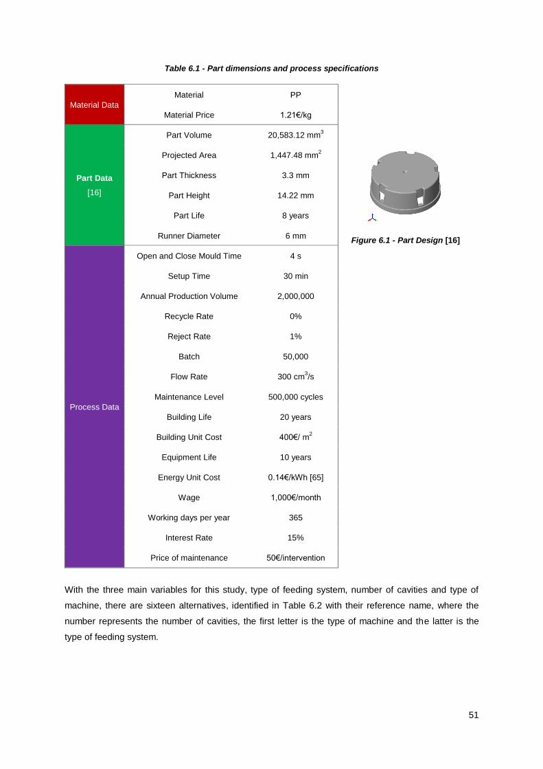
51
Table 6.1 - Part dimensions and process specifications
Material Data
Material PP
Figure 6.1 - Part Design [16]
Material Price 1.21€/kg
Part Data
[16]
Part Volume 20,583.12 mm3
Projected Area 1,447.48 mm2
Part Thickness 3.3 mm
Part Height 14.22 mm
Part Life 8 years
Runner Diameter 6 mm
Process Data
Open and Close Mould Time 4 s
Setup Time 30 min
Annual Production Volume 2,000,000
Recycle Rate 0%
Reject Rate 1%
Batch 50,000
Flow Rate 300 cm3/s
Maintenance Level 500,000 cycles
Building Life 20 years
Building Unit Cost 400€/ m2
Equipment Life 10 years
Energy Unit Cost 0.14€/kWh [65]
Wage 1,000€/month
Working days per year 365
Interest Rate 15%
Price of maintenance 50€/intervention
With the three main variables for this study, type of feeding system, number of cavities and type of
machine, there are sixteen alternatives, identified in Table 6.2 with their reference name, where the
number represents the number of cavities, the first letter is the type of machine and the latter is the
type of feeding system.

52
Table 6.2 – Mould Design and Type of machine alternatives: H – Hydraulic and E - Electric
Reference Name
Type of injection machine
Number of Cavities Type of Feeding
System
4H-C H 4
Cold Runners
4E-C E
8H-C H 8
8E-C E
12H-C H 12
12E-C E
16H-C H 16
16E-C E
4H-H H 4
Hot Runners
4E-H E
8H-H H 8
8E-H E
12H-H H 12
12E-H E
16H-H H
16 16E-H E
6.1.1 Resources Inventory
The model developed allows for the analysis of several intermediate outputs in the injection moulding
process. Still, it is only worth to study three of those outputs: amount of material, cycle time and
energy, as the first two are considered the most important outputs of this process, since material
consumption is high and cycle time controls many of the other parameters in the process, and energy
consumption, although not as significant as the material, is one of the parameters most injection
moulding companies are trying to reduce. Understanding these variables is vital to comprehending the
process, the resulting costs and environmental impact, and ultimately the Eco-efficiency of injection
moulding. All three variables will be analysed for the alternatives presented in Table 6.2.
The results for each variable are presented in Figure 6.2, Figure 6.3 and Figure 6.4, for both one part
and one injection moulding cycle, to better understand the influence of the number of cavities,
machine type and feeding system in the process.
It is chosen to present the following results from lowest to highest, in order to understand how each
mould design alternative and type of machine influences each variable, and the same distribution of
alternatives when analysing the same parameter.
Figure 6.2 illustrates the material consumption for all previous mould design alternatives, broke down
in material to form the part and engineering scrap, disregarding the setup scrap as the values are
insignificant when compared to the other results.

53
(a)
(b)
Figure 6.2 - Material quantity breakdown: (a) kg per part and (b) kg per cycle
The first conclusion taken from these results is that, only the alternatives with cold runners have
engineering scrap, meaning the additional material resulting from the type of feeding system. This
result is expected since, for hot runners, only the final part is ejected with no additional material.
Furthermore, it is important to note that the engineering scrap increases when measured per cycle,
maintaining a similar value when measured per part. This is due to the fact that, the number of
runners, with cold runners, increases with the number of cavities in order to fill every cavity.
Secondly, as the number of parts produced in one cycle increases with the number of cavities, the
amount of material also increases with the number of cavities, as expected. Finally, it is possible to
verify that the machine type has no influence in the material results, as expected.
Figure 6.3 illustrates the distribution of cycle time along the mould design alternatives, broke down in
filling, cooling and reset times, meaning the time to open and close the mould. When analysing these
results it is important to remember that the cooling time is dependent on the runner diameter for cold
runners and the part thickness for hot runners, and the reset time is established at 4s, independently
of feeding system, machine type or number of cavities.
0.018 0.019 0.020 0.021 0.022
16H-C16E-C16H-H16E-H12H-C12E-C12H-H12E-H8H-C8E-C8H-H8E-H4H-C4E-C4H-H4E-H
Material Consumption [kg/part]
material [kg/part] engineering scrap [kg/part]
0.000 0.100 0.200 0.300 0.400
16H-C16E-C16H-H16E-H12H-C12E-C12H-H12E-H8H-C8E-C8H-H8E-H4H-C4E-C4H-H4E-H
Material Consumption [kg/cycle]
engineered scrap [kg/cycle] material [kg/cycle]

54
(a)
(b)
Figure 6.3 - Cycle time: (a) time per part and (b) time per cycle
Results show that the cycle time, for one injection moulding cycle, is the same for all hot runner
alternatives, regardless of the number of cavities, since the cooling time is equal in all mould design
alternatives, as the part thickness is equal, and the increase in filling time, resulting from the increase
in material to be injected, is negligible. As the cycle time per part is the cycle time per injection
moulding cycle divided by the number of cavities, the cycle time per part decreases with the number of
cavities, as expected.
For cold runners, the filling time is no longer negligible, increasing with the number of cavities, as a
result of the increase in material to be injected, and the cooling time is constant, due to the constant
runner diameter established in this model. Hence the cycle time per injection moulding cycle increases
with the number of cavities. However, for one part, the reverse distribution is verified, where the cycle
time increases with the decrease in number of cavities, demonstrating the influence of cooling time in
the final result.
For all these results it is not demonstrated any influence of machine type, as expected, since, in this
model, the flow rate is constant, and independent of type of machine, defined at the start.
Figure 6.4 illustrates the distribution of energy consumption, both per part and per cycle, broke down
by thermodynamic and “machine” energy. To analyse these results one must have in mind that this
model defines the machine to be used, from a set of machines established at the start, according to
their maximum clamping force. As such, it is expected that all alternatives, with different number of
cavities, require different machines. However, in this case, both alternatives with eight and twelve
cavities use the same machine. Although this is not ideal to demonstrate the full use of the model
0 2 4 6 8
16H-C16E-C12H-C12E-C8H-C8E-C4H-C4E-C
16H-H16E-H12H-H12E-H8H-H8E-H4H-H4E-H
Cycle Time [s/part]
filling time [s/part] cooling time [s/part]
reset time [s/part]
0 10 20 30 40
16H-C16E-C12H-C12E-C8H-C8E-C4H-C4E-C
16H-H16E-H12H-H12E-H8H-H8E-H4H-H4E-H
Cycle Time [s/cycle]
filling time [s/cycle] cooling time [s/cycle]
reset time [s/cycle]

55
created for this work, it can be considered correct since, in reality, several mould design alternatives
can be used with the same machine, as long as it does not exceed the maximum clamping force.
(a)
(b)
Figure 6.4 - Energy consumption breakdown: (a) kWh per part and (b) kWh per cycle
Starting with the energy per part, it is possible to verify that all cold runner alternatives present a
higher energy consumption than the hot runner alternatives, as expected, allowing to conclude that the
type of feeding system has a more significant influence in these results than machine type or number
of cavities. To better understand these results, the thermodynamic and machine energy will be
discussed separately, for both types of feeding system.
In terms of thermodynamic energy, it is equal in all hot runner alternatives, independently of number of
cavities and machine type, due to the amount of material to melt and inject, being equal in all these
options, as only the mould cavity is filled. However, for cold runners, this value is now dependent on
the number of cavities, due to the additional material ejected with the part, but still independent on the
type of machine.
As for “machine” energy, meaning the energy consumed by the machine in all other stages of the
process, with the exception of melting and injecting, it presents no significant difference with the
number of cavities, for hot runners and the same machine type, since it is mainly dependent on the
cycle time and this does not change for these alternatives. Still, as hydraulic machines consume more
energy than electric ones, the alternatives with hydraulic machines will present a larger machine
consumption. For cold runners, the reasoning is the same and the distribution is similar, with the
hydraulic options consuming more machine energy. However, as the machine energy is dependent on
0 0.01 0.02 0.03 0.04 0.05
16H-C16E-C12H-C12E-C8H-C
16H-H8E-C
16E-H12H-H8H-H
12E-H4H-C8E-H4E-C4H-H4E-H
Energy Consumption [kwh/part]
thermodynamic energy [kWh/part]
machine energy [kWh/part]
0 0.2 0.4 0.6 0.8
16H-C16E-C12H-C12E-C8H-C
16H-H8E-C
16E-H12H-H8H-H
12E-H4H-C8E-H4E-C4H-H4E-H
Energy Consumption [kWh/cycle]
thermodynamic energy [kWh/cycle]
machine energy [kWh/cycle]

56
the thermodynamic energy, and the latter increases with the number of cavities, the machine energy
will also increase with the number of cavities.
When analysing the energy consumption per injection moulding cycle, the influence of the number of
cavities is more significant, with the thermodynamic energy, for hot runners, now being altered,
increasing with the number of cavities.
6.1.2 Cost Results
Having understood the resources results, it is now possible to discuss the cost results found with the
model developed.
Figure 6.5 illustrates the results in terms of cost per year, broke down by each individual costs, for all
alternatives of Table 6.2.
Figure 6.5 – Cost Breakdown for design alternatives
The first conclusion taken from these results is that, the most important factors for the injection
moulding costs, for this study, are associated with material and mould. Another conclusion is that,
independently of the type of machine, the material cost is similar for the same type of feeding system,
increasing from hot to cold runners, as expected. This fact is due to the amount of material needed for
the process, which the distribution is presented in Figure 6.2. In Figure 6.2 (b), the material
consumption increases with the number of cavities however, in Figure 6.5, the material cost has no
significant increase with the number of cavities, for the same feeding type, demonstrating the influence
of the number of cycles needed to produce the required production volume.
As for the mould cost, it is influenced by the mould’s dimensions and type of feeding. The cost
increases with the number of cavities, due to the increase in its dimensions, and with the type of
0 € 20,000 € 40,000 € 60,000 € 80,000 € 100,000 € 120,000 €
16H-C16E-C16H-H16E-H12H-C12E-C12H-H12E-H8H-C8E-C4H-C4E-C8H-H8E-H4H-H4E-H
Total Cost [€]
Material Cost Energy Cost Labour Cost Machine Cost
Tooling Cost Building Cost Maintenance Cost

57
feeding system, as a result of additional costs for hot runners. Although important, the mould cost will
not be analysed further since the behaviour is easily explained, as mentioned earlier, and only worth
being added that the mould life also has an influence in the mould cost, considering that moulds with
the same dimensions and type of feeding system will have a lower cost per year for moulds with a
higher mould life, as expected.
In terms of energy, for cold runners, the cost increases with the number of cavities and from electric to
hydraulic machines, and is identical for the same machine type, for hot runners, with no significant
influence with the number of cavities. This study for energy consumption is illustrated in Figure 6.4.
As for labour, machine and building costs, the main driver is cycle time, through the annual required
time. These results, although almost negligible for a higher number of cavities, should not be excluded
from any cost study due to their importance in the final result for lower production volumes and lower
number of cavities. For example, for some mould design alternatives, namely for four cavities, the
machine cost is as important as the energy cost, supporting the statement that these additional costs
should not be excluded from any study of injection moulding.
Maintenance cost could be discarded from this analysis since it is only present for four cavities, due to
the maintenance level of 500,000 cycles defined in this study and the decrease of cycles with the
increase of number of cavities. This means that, from four cavities on, the number of cycles to produce
the defined production volume is less than the maintenance level, hence there is no maintenance
intervention during production. Although this cost is not important in this analysis, it should be included
as the maintenance level can be changed, or different part characteristics can be defined, namely if
the part geometry is complex, if thin features are required and if the polymer is abrasive. These three
characteristics would increase the need for maintenance, as well as the total downtime, and modify
the labour, machine and building costs. In spite of the maintenance level being directly influenced by
the three part characteristics mentioned earlier, no direct relation was found. As such, the
maintenance level is a direct input for the user, leaving room for error.
An important note is that, as presented, with the increase of number of cavities, the time required per
year to fulfil the production volume decreases. As such, the cost per year increases with the increase
of number of cavities. However, it is possible that, for other production volumes, another mould design
alternative would be considered the best in terms of cost. The analysis of total cost for different
production volumes, for these mould design alternatives, is performed in Chapter 7.
6.1.3. Environmental Results
As explained in section 5.3, the environmental impact, for this study, is calculated as a sum of
individual impacts caused by energy, material, including the polymer to produce the part and the steel
to manufacture the mould, and the impact of waste which is the amount of polymer wasted in the
injection moulding process.

58
To calculate the environmental impact, the relevant information is retrieved from the model and
weighed with the aid of the SimaPro software, which attributes a specific impact according to the Eco-
indicator used, in this case ReCiPe.
Table 6.3 illustrates the specific impact for each contributing factor.
Table 6.3 – Specific Impact from SimaPro [Pts]
PP Incineration Energy Steel
Specific Impact 0.315 Pts/Kg 0.013 Pts/kg 0.051 Pts/kWh 1.4 Pts/kg
Figure 6.6 illustrates the environmental impact breakdown.
Figure 6.6 - Environmental Impact Breakdown
These results indicate that the material is the most contributing factor to the overall environmental
impact, followed by the energy impact. The explanation for these values can be related to the resource
inventory, namely Figure 6.2 and Figure 6.4, where the results for the amount of material and energy
are presented and commented in terms of number of cavities, type of feeding system and machine
type.
It is interesting to note that, although the specific impact of the mould material is high, the total
environmental impact caused by the mould is negligible. This is caused by the amount of steel to form
the mould, which is extremely lower than the amount of material to form the parts.
In this study it is considered that all material waste is incinerated, as it was chosen to present the
worst case scenario, and to consider a percentage of recycling would not give additional information,
although it is the most common practice. This impact is caused by the wasted material in the runners,
hence it is only present in the cold runner alternatives.
0 5000 10000 15000 20000
16H-C16E-C16H-H16E-H12H-C12E-C12H-H12E-H8H-C8E-C4H-C4E-C8H-H8E-H4H-H4E-H
Environmental Impact [Pts]
Material [Pts/kg] Energy [Pts/kWh] Mould [Pts/kg] Incineration [Pts/kg]

59
6.2 Eco-efficiency
Having understood the potential of the PBM and the results, in terms of resources, costs and
environmental impact, it is now possible to estimate the Eco-efficiency, for all alternatives presented in
Table 6.2. Since the Eco-efficiency indicators can be general or specific, the ratios will be calculated
for both indicators.
The first step is to understand what indicators make sense for this study and how they can be
calculated. Finally, the Eco-efficiency indicator can be estimated and analysed.
As Eco-efficiency can be calculated through general or specific indicators, it is important to
demonstrate how the model developed for this work can calculate Eco-efficiency, with both types of
indicators for the mould design alternatives presented in Table 6.2. To present the following results,
for general indicators, the same mould design alternatives distribution is used as presented in Figure
6.5, and for specific indicators, the mould design alternatives will be presented from lowest to highest.
Furthermore, as the Eco-efficiency Ratio translates value per environmental impact, for general
indicators, and this work is mainly focused on the comparison of mould design alternatives, in addition
to this study not being based on a specific company, hence not having its respective financial
information, both the value indicators and environmental impact will be normalized, based on one
reference alternative.
6.2.1 Added Value (Normalized Cost Results)
“Value is created whenever benefits exceed the costs” [54]. As such, and according to standards,
there are several economic indicators that can translate this value.
As this model, although for use in injection moulding companies, is mainly for the comparison between
different mould designs, without relying on specific business information, as for example revenues, the
economic indicators need to be adapted from the indicators presented in Chapter 4. To overcome this
fact, the following results for each indicator will be presented as differentials in the form of a ratio,
𝐶𝑟𝑒𝑓 𝐶𝑖⁄ , where 𝐶𝑖 is the cost for alternative i and 𝐶𝑟𝑒𝑓 is the cost for the reference alternative, allowing
to compare the value between different mould design alternatives and a reference design, established
as the alternative with the lowest cost and, therefore, the highest added value.
Disregarding the company information, the revenues, the calculations for the GVA and NVA,
Equations (4.1) and (4.2), will be made according to Equations (6.1) and (6.2), where 𝐼𝐺𝑉𝐴 and 𝐼𝑁𝑉𝐴 are
the indicators corresponding to GVA and NVA respectively, used for this work.
GVAI = Non-factor costs = Material Cost + Energy Cost (6.1)
NVAI = Internal Costs + External Costs = Total Cost (6.2)

60
As previously mentioned, the mould design alternatives will be compared, using as a reference, the
best option in terms of cost. From Figure 6.5 it is concluded this alternative is four cavities, electric
machine and hot runners (4E-H), as it translates to the highest added value.
Figure 6.7 illustrates the results, in terms of 𝐼𝐺𝑉𝐴, for the various alternatives, normalized for the 4E-H
option.
Figure 6.7 - 𝑰𝑮𝑽𝑨 Results (normalized) for the various alternatives
As expected, all hot runner alternatives have the highest GVA indicator, indicating they have the
highest added value, since the material cost is the most influential cost in these results. The
explanation for the differences in results between these alternatives, for both material and energy, is
presented in section 6.1.
Having understood the influence of material and energy cost in the final result, it is now time to include
all other costs and analyse their influence in the added value results. Figure 6.8 illustrates the 𝐼𝑁𝑉𝐴
results, for the various alternatives, normalized for the same mould design alternative, 4E-H.
Figure 6.8 - 𝑰𝑵𝑽𝑨 Results (normalized) for the various alternatives
0
0.2
0.4
0.6
0.8
1
𝐼𝐺𝑉𝐴
no
rma
lize
d
Material Cost (normalized) Energy Cost (normalized) Reference
0
0.2
0.4
0.6
0.8
1
𝐼𝑁𝑉𝐴
no
rmalized
Material Cost (normalized) Energy Cost (normalized)
Labour Cost (normalized) Machine Cost (normalized)
Tooling Cost (normalized) Building Cost (normalized)
Maintenance Cost (normalized) Reference

61
An important note is that these costs are normalized with the 𝐼𝑁𝑉𝐴 results, as opposed to the 𝐼𝐺𝑉𝐴
results presented previously. As such, although the material costs are equal for both indicators, the
results, when normalized, will be different when compared to the results presented in Figure 6.7. Still,
the material cost continues to be the most influential parameter in these analyses.
The second most meaningful parameter is mould cost, as expected from Figure 6.5. Having in mind
the ratio used to normalized this values and the costs previously presented, it is explained the
increase in normalized costs along the mould design alternatives as presented, hence increasing the
added value.
A final note on these results is that the distribution follows the one presented in Figure 6.5, as
expected, with the alternatives with the highest cost being the mould design options with the lowest
added value.
6.2.2 Normalized Environmental Impact Results
As the Added Value Results are normalized, it is also required to normalize the Environmental Impact
Result. Following the ratio 𝐸𝐼𝑖 𝐸𝐼𝑟𝑒𝑓⁄ , Figure 6.9 illustrates the environmental impact results from
section 6.1.3, normalized also using 4E-H as a reference. Any alternative with a higher ratio than the
reference will indicate a higher environmental impact.
The reasoning behind these results has already been presented in section 6.1.3.
Figure 6.9 - Environmental Impact Results (normalized) for the various alternatives
As expected, the hot runner alternatives present the ratio closest to the reference, due to the identical
material consumption. Hence, it is expected that these alternatives will represent the best mould
design options in terms of environmental impact.
0
0.2
0.4
0.6
0.8
1
1.2
1.4
EI (n
orm
alized
)
Material Energy Mould Incineration Reference

62
6.2.3 Eco-Efficiency Ratio Results – General Indicators
With the Added Value and Environmental Impact Results normalized, it is now possible to present the
Eco-Efficiency Results following the Eco-Efficiency Ratio, Equation (6.3), as presented in Chapter 3.
ValueEco-Efficiency Ratio =
Environmental Impact (6.3)
Since both the 𝐼𝐺𝑉𝐴 and 𝐼𝑁𝑉𝐴 were discussed previously, relaying important differences in the cost
results, the Eco-Efficiency Ratio is presented for both results, for the various design alternatives. To
better understand the outcome, both the 𝐼𝐺𝑉𝐴 results, or 𝐼𝑁𝑉𝐴 results, and EI results are presented in
association with the Eco-efficiency Ratio results.
The following results are normalized, using 4E-H as the reference, since both the cost and
environmental impact results were normalized for the same mould design alternative and presented
from lowest to highest.
Figure 6.10 presents the Eco-efficiency Ratio for the 𝐼𝐺𝑉𝐴 results.
Figure 6.10 – Normalized Eco-Efficiency Results for 𝑰𝑮𝑽𝑨 Results
These results indicate that the normalized Eco-Efficiency Ratio is similar to the reference, for all hot
runner alternatives, as expected, since both the added value and environmental impact results
normalized present the closest values to the reference for these alternatives. It is also important to
note that the EI normalized and GVA indicator normalized exhibit an inverse distribution, since when
the former increases, the latter decreases. The EI distribution is also presented as higher than the
reference due to the different ratio used to normalize the values.
Furthermore, taking per example alternatives 16H-H and 16E-H, the material cost and the
environmental impact caused by the material is equal, since the amount of material used is equal in
both alternatives. The differences demonstrated are due to the energy impact in both cost and
environmental impact, where the influence is greater in the added value. As such, the Eco-efficiency
0.00
0.20
0.40
0.60
0.80
1.00
1.20
1.40
1.60
EE
(n
orm
alized
)
Eco-Efficiency normalized IGVA normalized
EI normalized Reference

63
Ratio is be greater for the alternatives with electric machines, as these consume less energy, as
previously discussed.
Summing, all hot runner alternatives will result in a higher Eco-efficiency Ratio, when compared to
cold runner alternatives, as a result of the decrease in material consumption, and the alternatives with
electric machines will also result in a higher Eco-efficiency Ratio, compared to hydraulic alternatives,
due to the decrease in energy consumption.
Still, Eco-efficiency presented in such a way can lead to error as different values for added value and
EI can lead to a similar ratio, as is the case of hot runners where the Eco-efficiency Ratio results are
equal, for this case study, for several mould design alternatives. This can be problematic since the
goal of this work is to analyse which is the best alternative in terms of mould design.
To comprehend these results a different approach is taken, positioning all mould design alternatives in
terms of 𝐼𝐺𝑉𝐴 and Environmental Impact. Figure 6.11 illustrates all mould design alternatives,
positioning each circle in order to indicate the best and worst alternatives in terms of Eco-efficiency. In
these results, the circle’s dimensions indicate the normalized Eco-efficiency Ratio result.
Figure 6.11 - 𝑰𝑮𝑽𝑨 (normalized) vs. Environmental Impact (normalized)
The importance of presenting the Eco-efficiency results in such a way, in this case, is only clear in the
cold runner alternatives since the hot runners alternatives cannot be clearly distinguished. Still, if the
cold runners alternatives were excluded, the remaining would be distinguishable, and this method of
presenting the results more significant.
Still, the overall conclusion for these results remains that all hot runner alternatives exibit the highest
Eco-efficiency Ratio, hence are the best alternatives in terms of EE.
0.9
1
1.1
1.2
1.3
1.4
1.5
0.7 0.75 0.8 0.85 0.9 0.95 1 1.05 1.1
En
vir
on
men
tal
Imp
act
[Pts
] (
no
rmalized
)
𝐼𝐺𝑉𝐴 [€] (normalized)
Low EE
High EE
Hot Runners
16H-C
12H-C
16E-C
8H-C
12E-C
8E-C 4H-C
4E-C

64
Having analysed the Eco-efficiency results for the 𝐼𝐺𝑉𝐴, it is now time to study the same mould design
alternatives in terms of the 𝐼𝑁𝑉𝐴, in order to investigate if the same distribuition is presented with both
cost alternatives. Figure 6.12 illustrates the results of this study.
Figure 6.12 – Normalized Eco-Efficiency Results for 𝑰𝑵𝑽𝑨 Results
In this figure, the environmental impact has the same distribuition as presented in Figure 6.10, as
expected, since there is no difference in the calculations. However, the Eco-efficiency Ratio will
present different results, comparing to the results of Figure 6.10, due to the different value indicators
used in both analysis.
It is important to note that the normalized EE Results are substancialy lower than the reference, until
alternative 8H-H, due to the difference between the normalized EI results and the normalized NVA
indicator,which is considerable until this alternative.
To further analyse this ratio, the same tool as presented in Figure 6.11 is used, positioning each
design alternative in terms of 𝐼𝑁𝑉𝐴 and Environmental Impact. Figure 6.13 illustrates the results of this
analysis.
0.00
0.20
0.40
0.60
0.80
1.00
1.20
1.40
1.60
EE
(n
orm
alize
d)
Eco-efficiency normalized INVA normalized
EI normalized Reference

65
Figure 6.13 - 𝑰𝑵𝑽𝑨 (normalized) vs. Environmental Impact (normalized)
It is now verified the usefulness of this tool to evaluate the best alternative when the Eco-efficiency
Ratio is equal, as is the case of alternatives 8E-H and 4H-H, where the latter has the highest added
value but also the highest environmental impact. With these results it is demonstrated the importance
of calculating the Eco-efficiency Ratios, but also to use a tool where each alternative is positioned, in
relation to the others, and evaluated, not based solely on the ratios.
Comparing Figure 6.10 and Figure 6.12, the main difference is presented for hot runners, where the
added value between alternatives with different number of cavities is no longer similar, as a result of
the added mould cost. It is also important to note that the alternatives are almost presented in pairs,
with the hydraulic machine alternatives always inducing a higher cost due to energy consumption, and
the difference between options, for the same machine type, is mainly caused by material consumption
and mould cost for cold runners, and solely by mould cost for hot runners.
6.2.4 Eco-efficiency Ratio Results – Specific Indicators
Until this point, Eco-efficiency has been studied, in this work, through general indicators, defined by
the ratio between added value and environmental impact. As an example of a few specific indicators,
the Eco-efficiency of each mould design alternative will be presented as the ratio between annual
required time, energy and wasted material, and the amount of material injected.
Figure 6.14 illustrates the results for this study.
0.9
1
1.1
1.2
1.3
1.4
1.5
0.65 0.7 0.75 0.8 0.85 0.9 0.95 1 1.05
En
vir
on
me
nta
l Im
pa
ct
[Pts
] (n
orm
alize
d)
𝐼𝑁𝑉𝐴 [€] (normalized)
Low EE
High EE
16H-C
16E-C
12H-C
12E-C
8H-C
8E-C
4H-C
4E-C
16H-H
16E-H
12H-H
12E-H
8H-H
8E-H
4H-H
4E-H

66
(a)
(b)
(c)
Figure 6.14 - Eco-Efficiency Results for Specific Indicators: a) Annual Required Time; b) Energy and c)
Material Waste
The reasoning behind these results has already been established in section 6.1, when the three main
resources from the PBM were explained. Still, it is important to perform this analysis, with specific
indicators, as the information relayed is better understood by the mould designer. As the main
objective of mould designers it to reduce cycle time and material and energy consumption, without
compromising on quality, these ratios would be useful and more easily comprehended than the
General Indicators presented in section 6.2.3, which are more important at a management level.
0 0.05 0.1 0.15
16H-C16E-C12H-C12E-C8H-C8E-C4H-C4E-C
16H-H16E-H12H-H12E-H8H-H8E-H4H-H4E-H
Material Waste [kg/year]/ Material Injected [kg/year]
0 0.02 0.04 0.06 0.08
4H-C4E-C4H-H4E-H8H-C8E-C8H-H8E-H
12H-C12E-C12H-H12E-H16H-C16E-C16H-H16E-H
Annual Required Time [h/year]/ Material Injected [kg/year]
0 0.5 1 1.5 2
16H-C12H-C16E-C8H-C
12E-C8E-C4H-C4E-C4H-H
16H-H8H-H
12H-H4E-H8E-H
16E-H12E-H
Energy [kWh/year]/ Material Injected [kg/year]

67
7 Proposed Methodology for EE Comparison and Sensitivity
Analysis
In this chapter, is described the proposed methodology to compare the performance of different mould
design alternatives, in terms of Eco-efficiency, for the same part.
Along with the analysis of resources, costs, environmental impact and Eco-efficiency, it is also
possible to perform a sensitivity analysis, where it will be studied the influence of production volume
on the total cost and the influence of thickness in the total cost and environmental impact.
Before any analysis the user must:
Define the variables of Part Data, presented in Annex A
Introduce the machining times for each manufacturing process of the mould cavity, for one
cavity, and the cost per hour of each process. Introduce all additional costs for the mould such
as accessories, thermal treatments, etc.
The databases for material, mould plate dimensions and machines are already established with a few
examples. Still, the user can modify the values for each variable, according to the company or market
specifications, or define additional entrees.
It is important to define the databases of mould and machine since the model will choose, between the
options defined, the best in terms of the clamping force for the machine and mould dimensions for the
mould. It should be noted that, when conducting studies with this model, designers need to have
sensitivity to mould and machine parameters in order to guarantee that the necessary mould and
machine dimensions are defined in the databases.
To start any analysis the user must:
Define the unit costs for energy and building and life for the machine, building and part, the
salary, number of workers per machine, interest rate and number of working days per year
Choose the material from the corresponding database
Define the production volume, batch, number of cavities, flow rate, recycle rate, reject rate
Choose the type of machine (electric or hydraulic) and type of feeding system (hot runners or
cold runners)
Define, according to chosen part and material, if it has complex geometry, thin features and
abrasive material, and indicate the maintenance level.
With these steps a resource inventory is created, indicating, per example, the part weight, cycle time
and annual required time, and the costs for material, energy, labour, machine, mould, building and
maintenance are directly calculated.

68
Apart from the previous variables, the model also allows for the user to specify certain values which, if
left undefined, are calculated directly by the model. These variables are:
Total Downtime
Setup time
Open and close mould time
Cycle time per shot
Scrap per setup
Engineering scrap
Mould life
Revenues, which is only used if defined, since the model has no way to calculate this variable
To evaluate the environmental impact, the user has only to establish what resources are to be studied,
from the resources inventory. If a different resource, other than polymeric material and waste, energy
and mould material, is to be considered, the user must also indicate the specific environmental impact
for that resource, found in the software SimaPro.
As the main objective of this model is to compare mould design alternatives in terms of Eco-efficiency,
the resources, costs and environmental impact results need to be taken for each mould design,
modifying the number of cavities and the type of feeding system, in order to calculate the Eco-
efficiency for each mould alternative.
To obtain the Eco-efficiency Ratios, for each mould design alternative and general indicators, the user
must obtain the added value results, from the cost results, and the environmental impact results,
whereas for specific indicators, the user can take the desired valued from the resources inventory, and
calculate the Eco-efficiency Ratio according to standards, with no need to normalize the results.
Figure 7.1 illustrates the information flow along the PBM, indicating the variables to be defined by the
user, the results and analysis the model is able to perform and, additionally, the influence between
variables and the databases already established. It is important to note that, for the environmental
impact analysis, a few additional parameters could be added if the user has that information as, for
example, the mould waste, meaning the material wasted in mould production.

69
Analysis
Resources CostsEnvironmental
ImpactEco-efficiency
Material
Energy
Labour
Machine
Tooling
Building
Maintenance
Material
Energy
Labour
Machine
Tooling
Building
Maintenance
Plastic material
Plastic waste
Energy
Mould material
General indicators
Specific indicators
Part Data
Geometry
Complexity
Part Life
Mould Plate
Database
Material
Database
Machine
Database
Resource
Inventory
Resources
Costs
Environmental
Impact
Specific
Environmental
Impact
Price
Factors
Mould Data
Number of
Cavities
Type of Feeding
System
Injection Data
Production Volume
Batch
Flow Rate
Recycle Rate
Rejection Rate
Machine Type
Machine Life
Building Life
No. Workers per machine
No. Working days per year
Comparison of Mould Design Alternatives
Sensitivity Analysis
Influence Information Flow
Figure 7.1 – Proposed Methodology for EE Comparison
Apart from these analyses, it is also possible to perform a sensitivity analysis to certain parameters
such as production volume and part dimensions, as indicated in Figure 7.1. To demonstrate the
possible results of these analyses, the part cost variation with the production volumes and the part
cost and total environmental impact variation with the part thickness will be studied.
All cost analysis in this study are presented as total cost per part, to better demonstrate the variations,
and the environmental impact is presented as a total for the production volume, since the values per
part do not present a significant difference.

70
Figure 7.2 illustrates the results of the sensitivity analysis of part cost with the production volume. For
this study it was chosen to analyse only the alternatives with electric machines, as the difference in
cost between hydraulic and electric machines has already been presented. To simplify the analysis of
the results, only the best alternatives are presented, meaning the alternative with the lowest total cost,
for the interval of production volume values.
Figure 7.2 – Variation of Cost per part with the Production Volume
These results indicate that, for low production volumes, until approximately 500,000 parts, cold
runners present a lower cost than any hot runner alternatives, since the mould cost for cold runners is
lower than for hot runners, and all other costs do not compensate this difference.
Increasing the production volume, the statement that there is a certain production volume where a
higher number of cavities presents a lower cost, written in Chapter 6, is validated. It is important to
note that, alternative 4E-H presents the lowest cost until a production volume of 2,500,000 parts,
approximately, hence it is explained why this alternative is considered the best, in terms of cost, for
the cost results of Chapter 6, where the production volume is 2,000,000 parts.
Having understood influence of the production volume in the part cost, it is now presented the analysis
for different thickness values, maintaining all other part dimensions and process characteristics, as
defined in Table 6.1. The main objective of this study is to demonstrate how the model developed
reacts to variations of part thickness, not being a particularly useful study for mould designers.
Figure 7.3 illustrates the results of the analysis of part cost variation with part thickness, for alternative
4E-H and a production volume of 2,000,000 parts.
0
0.01
0.02
0.03
0.04
0.05
0.06
0.07
0.08
500 5,000,500 10,000,500 15,000,500 20,000,500 25,000,500 30,000,500
To
tal C
os
t [€
/pa
rt]
Production Volume

71
Figure 7.3 - Variation of Cost per part with Part Thickness for 2,000,000 parts and alternative 4E-H
These results indicate that the cost per part increases with the part thickness, due to the influence of
thickness in the energy consumption, where an increase in thickness will result in an increase in CfT,
energy thickness coefficient, and in the cycle time. However, until a thickness of approximately 0.4
mm, the CfT has a much higher influence in the energy consumption, hence the energy cost
decreases. The relation between CfT, cycle time and energy consumption is presented in Equation
(5.18). Still, as the cycle time increases, labour, machine and building costs increase, compensating
the decrease in energy cost. Hence the part cost, until 0.4 mm, appears almost stable.
From a thickness of 0.4 mm, the cycle time exhibits a much higher influence in the energy
consumption. Hence the energy cost will increase, along with all other costs. Since the material and
mould costs are not influenced by the part thickness, for this model, both these costs will remain
stable.
Furthermore, there is a discrepancy in total cost results for 3 mm thickness. This can be explained by
the part thickness coefficient, k, presented in Equation (5.24), where the coefficient value is modified
for a thickness of 3 mm. As such, for higher thickness values, the total cost per part will have a more
significant increase with thickness.
These results are only valid for hot runners, since the cycle time, for cold runners, is not influenced by
the part thickness, in this model, and the material and mould costs remain stable as previously stated.
As such, the cost per part, for cold runners, will decrease steadily with the decrease in energy cost,
due to the increase in CfT.
In terms of environmental impact, defined in Chapter 6 as the sum of the individual impacts of material
and energy consumption, material waste and mould material, Figure 7.4 illustrates the influence of
part thickness on the total environmental impact.
0.026
0.027
0.028
0.029
0.03
0.031
0.032
0.033
0.05 0.6 1.15 1.7 2.25 2.8 3.35 3.9 4.45 5
To
tal C
os
t [€/p
art
]
Thickness [mm]
3 0.4
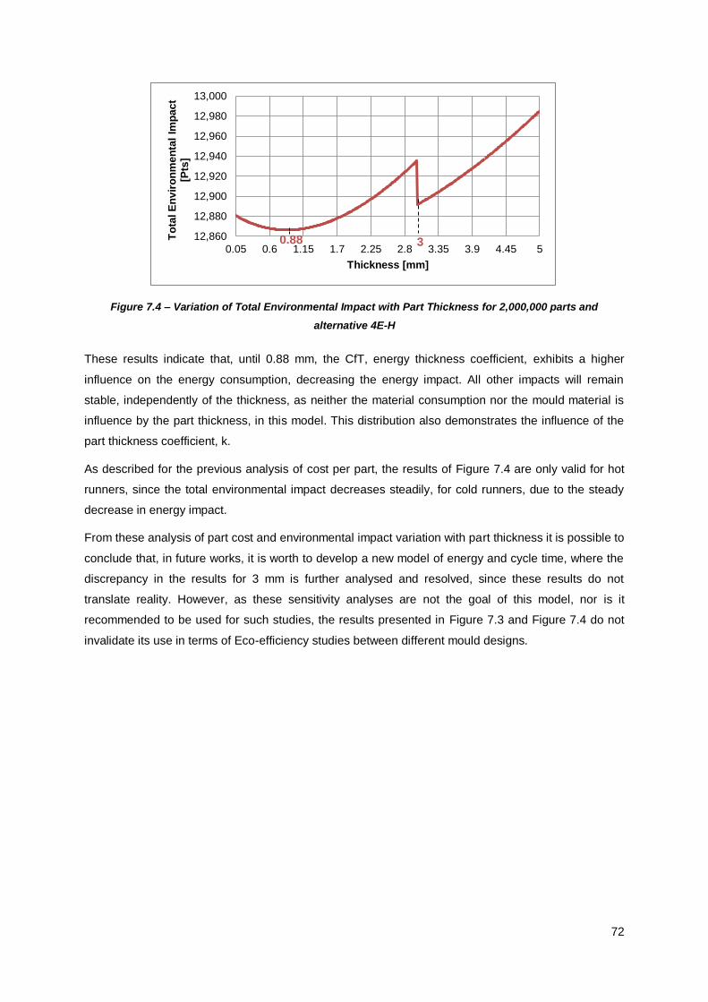
72
Figure 7.4 – Variation of Total Environmental Impact with Part Thickness for 2,000,000 parts and
alternative 4E-H
These results indicate that, until 0.88 mm, the CfT, energy thickness coefficient, exhibits a higher
influence on the energy consumption, decreasing the energy impact. All other impacts will remain
stable, independently of the thickness, as neither the material consumption nor the mould material is
influence by the part thickness, in this model. This distribution also demonstrates the influence of the
part thickness coefficient, k.
As described for the previous analysis of cost per part, the results of Figure 7.4 are only valid for hot
runners, since the total environmental impact decreases steadily, for cold runners, due to the steady
decrease in energy impact.
From these analysis of part cost and environmental impact variation with part thickness it is possible to
conclude that, in future works, it is worth to develop a new model of energy and cycle time, where the
discrepancy in the results for 3 mm is further analysed and resolved, since these results do not
translate reality. However, as these sensitivity analyses are not the goal of this model, nor is it
recommended to be used for such studies, the results presented in Figure 7.3 and Figure 7.4 do not
invalidate its use in terms of Eco-efficiency studies between different mould designs.
12,860
12,880
12,900
12,920
12,940
12,960
12,980
13,000
0.05 0.6 1.15 1.7 2.25 2.8 3.35 3.9 4.45 5
To
tal E
nv
iro
nm
en
tal
Imp
ac
t [P
ts]
Thickness [mm]
3 0.88
73
8 Conclusions
The main focus of this work was to create a tool to assist designers in an early design phase, in terms
of mould design alternatives, demonstrating how different mould designs can influence the Eco-
efficiency of the injection moulding process, for the same part and process variables, supporting the
statement that Eco-efficiency should be taken into consideration as early as possible to guarantee that
the best design option is chosen. To calculate the Eco-efficiency, it was necessary to first find the
costs and environmental impact for each mould design and machine alternative, based on a resource
inventory.
The Process Based Model developed for this works starts with a PBCM, relating the process, part,
mould and machine input variables to the final costs. With this tool it was possible to create a resource
inventory, understanding what variables are important for the injection moulding process, and how to
use these resources to find the final cost, allowing for a better understanding of the process and the
main cost drivers.
With the resources inventory of the PBM, for polymeric and mould material, polymeric waste and
energy, it was determined the environmental impact, multiplying each individual impact by their
specific environmental factor, found in SimaPro.
To present the results, several mould design alternatives were considered and analysed in terms
resources, in this case material and energy consumption and cycle time, costs and environmental
impact. From the cost analysis it was concluded, as expected, that the main cost drivers are material
and mould and that electric machines, although more expensive in terms of purchase price, will
compensate in energy consumption, hence having a lower total cost. In terms of environmental
impact, material consumption is the most contributing factor, for the defined production volume, even
though it does not have the highest specific impact. Between the mould alternatives studied, it was
established that the alternative with the lowest cost and environmental impact was 4E-H (four cavities,
with electric machine and hot runners).
As the goal it to present Eco-efficiency results, the costs were normalized, comparing each
alternatives with a reference, defined as the alternative with the lowest cost (4E-H), to obtain the
added value. With these results and the environmental impact results, also normalized with the same
alternative, the EE results were presented.
From bibliography it was defined that alternatives with a higher Eco-efficiency Ratio are established as
the best alternatives. These ratios allow designers to make critical decisions in the mould design
phase, without significantly increasing production costs, and facilitate the translation of important
information and performance comparison of different designs, mainly for Specific Indicators. Still,
although extremely important, taking decisions solely based on Eco-efficiency Ratios can be
misleading, since different values of Added Value and Environmental Impact can lead to the same
ratio, not necessarily meaning both alternatives are equal. Hence, in this work, the EE Results were
presented with a different method, positioning each alternative in terms of cost and environmental

74
impact, but also relaying the Eco-efficiency Ratio. With the results presented thus, it was possible to
verify that the alternative with the highest added value and lowest environmental impact, 4E-H, was
indeed the best alternative in terms of EE, even though other alternatives presented similar Eco-
efficiency Ratios.
It is also presented the proposed methodology for this study, explaining how the model should be
used and the flow of information along the model, resulting in the analyses of resources, costs,
environmental impact and EE. An additional analysis was performed, the sensitivity analysis, where
the part dimensions, in this case the thickness, and production volume are modified, and the costs and
environmental impact are studied. This analysis was especially useful to validate the affirmation that
the same mould design alternative does not present the lowest cost when the production volume is
increased and, in terms of thickness, that new models of energy and cycle time should be created,
since the current model presents a few discrepancies and does not fully translate reality. Still, as this
is not the recommended use of the model, these discrepancies should not invalidate the results
presented in terms of Eco-efficiency.

75
9 Future Work
In this chapter, a few suggestions for future work are presented.
A first suggestion is the values of setup time and reset time, time to open and close the mould, and the
flow rate, which are now treated solely as input variables but should be related, scientifically, to other
parameters, mainly to the machine use. For this, it should be created a model relating the setup and
reset times to the mould dimensions and machine parameters. In terms of flow rate, it should be
related to machine and mould parameters, but also to part dimensions and visual and performance
requirements. To evaluate these relations, it should be measured the values for these variables for
different settings and, with these values, create the models.
Secondly, in terms of mould, the diameter of the runners should not be treated as a constant, but
dependent on the flow rate, mould dimensions and part to be produced. As for the mould dimensions,
since the spacing between cavities is not a constant, usually raging between 100 and 120 mm
between part centres, and there are several possible distributions of cavities within a mould, for the
same number of cavities, there should be a specific relation between number of cavities, the part’s
projected area and the necessary mould dimensions, finding the best distribution of the cavities along
the mould. For this, there should be discussions with specialists in the area and created an equation
applicable to every study, indicating the best distribution of cavities along the mould to minimize the
mould dimensions, saving on material and energy and, ultimately reducing costs and environmental
impact.
A third suggestion is relating the part thickness to the part weight, thus relating to the amount of
material needed, since it is now only dependent on the projected area and part height. Also for this
variable, it should be created/found more precise models relating energy and cycle time to part
thickness in order to better translate reality, as was indicated in Chapter 7.
As this model is to be used in any injection moulding company, the mould dimensions and machines
database should be expanded, in order to attribute this data more accurately for the part and
alternatives do be studied.
Another suggestion is to conduct a broader study on environmental impact, including parameters such
as material wasted in mould production and the part’s end-of-life, which may contribute significantly to
the final results. In terms of Eco-efficiency, it is suggested to perform a broader study on Specific
Indicator, evaluating what parameter designers are more interested in studying.
Finally, it is suggested to use this model in an actual company, specifying all variables, and evaluating
if the same conclusions in terms of Eco-efficiency are found, especially considering there is no need to
normalize the cost values, as there is access to the company’s financial information on revenues.

76
References
[1] A. Baptista, E. Lourenço, J. Pereira, F. Cunha, B. Marques, E. Silva and P. Peças, “Eco-
Efficiency Framework as a Decision Support Tool to Enhance Economic and Environmental
Performance of Production Systems,” in Results from the Cluster of Excellence eniPROD, 3rd
workbook of the cross-sectional group ‘Energy-related technical and economic evaluation’ of the
Cluster of Excellence eniPROD, Auerbach, 2014.
[2] K. Madden, R. Young, K. Brady and J. Hall, Eco-Efficiency Learning Module, Five Winds
International, 2006.
[3] S. Apichartpattanasiri, J. N. Hay and S. N. Kukureka, “A study of the tribological behaviour of
polyamide 66 with varying injection-moulding parameters,” in Wear, Elsevier, 2001, pp. 1557-
1566.
[4] B. Ozcelik and T. Erzurumlu, “Comparison of the warpage optimization in the plastic injection
molding using ANOVA, neural network model and genetic algorithm,” Journal of Materials
Processing Technology, vol. 171, p. 437–445, 2006.
[5] R. Hussin, R. M. Saad, R. Hussin and M. S. I. M. Dawi, “An Optimization of Plastic Injection
Molding Parameters Using Taguchi Optimization Method,” Asian Transactions on Engineering,
pp. 75-80, 2012.
[6] “The History of Plastic Moulding,” [Online]. Available: http://www.plasticmoulding.ca/history.htm.
[Accessed March 2015].
[7] P. H. Kauffer, “Injection Molding: Process, Design, and Applications,” [Online]. Available:
https://www.novapublishers.com/catalog/product_info.php?products_id=17273. [Accessed March
2015].
[8] “Engineers Edge: Solutions by Design,” [Online]. Available:
http://www.engineersedge.com/manufacturing/injection-molding-applications.htm. [Accessed
March 2015].
[9] “The Portuguese Mould Industry,” [Online]. Available:
http://www.cefamol.pt/cefamol/en/Cefamol_IndustriaMoldes/Historia. [Accessed March 2015].
[10] D. M. Bryce, Plastic Injection Molding: Manufacturing Process Fundamentals, Society of
Manufacturing Engineers, 1996.
[11] M. V. Kavade and S. D. Kadam, “Parameter Optimization of Injection Molding of Polypropylene
by using Taguchi Methodology,” Journal of Mechanical and Civil Engineering, vol. 4, pp. 49-58,
2012.
[12] R. A. Malloy, “Prototyping and Experimental Stress Analysis,” in Plastic Part Design for Injection
Molding - An Introduction, Hanser, 2011, pp. 285-339.
[13] M. Khan, S. K. Afaq, N. U. Khan and S. Ahmaad, “Cycle Time Reduction in Injection Molding
Process by Selection of Robust Cooling Channel Design,” 2014. [Online]. Available:

77
http://www.hindawi.com/journals/isrn/2014/968484/. [Accessed March 2015].
[14] T. Kimerling, Injection Molding Cooling Time Reduction and Thermal Stress Analysis, Amherst,
Massachusetts, 2002.
[15] I. Pires, Moldação por Injecção: Class Notes, Instituto Superior Técnico, 2014.
[16] “Injection Molding,” 2007. [Online]. Available: http://www.custompartnet.com/wu/InjectionMolding.
[Accessed March 2015].
[17] D. V. Rosato, D. V. Rosato and M. G. Rosato, Injection Molding Handbook, 3ª ed., USA: Kluwer
Academic Publishers, 2000.
[18] R. H. Todd, D. K. Allen and L. Alting, Manufacturing Processes Reference Guide, Industrial
Press Inc., 1994.
[19] D. V. Rosato, M. G. Rosato and D. V. Rosato, Concise Encyclopedia of Plastics, USA: Springer
Science & Business Media, 2000.
[20] “Plastipedia,” British Plastics Federation, 2015. [Online]. Available:
http://www.bpf.co.uk/plastipedia/processes/Injection_Moulding.aspx. [Accessed March 2015].
[21] A. Thiriez, “An Environmental Analysis of Injection Molding,” Master Thesis in Mechanical
Engineering, Massachusetts Institute of Technology, USA, 2004.
[22] D. Godec, M. Rujnić-Sokele and M. Šercer, “Energy Efficient Injection Moulding of Polymers,” in
Acta Technica Corviniensis - Bulletin of Engineering, Zagreb, 2012.
[23] D. Godec, M. Rujnić-Sokele and M. Šercer, “Processing parameters influencing energy efficient
injection moulding of plastics and rubbers,” Polimeri: Plastics and Rubber Journal, vol. 33, pp.
112-117, 2013.
[24] I. Ribeiro, P. Peças and E. Henriques, “Incorporating tool design into a comprehensive life cycle
cost framework using the case of injection molding,” Journal of Cleaner Production, vol. 53, pp.
297-309, 2013.
[25] A. Thiriez e T. Gutwski, “An Environmental Analysis of Injection Molding,” em Proceedings of the
2006 IEEE International Symposium on Electronics and the Environment, San Francisco, 2006.
[26] M. Sklyarova and T. Kobets, “Eco-Efficiency for Sustainability: IKEA's environmental policy in
Russia,” Master Thesis in Business Administration, Gotland University, Sweden, 2011.
[27] J. Woodson, “Benchmarking a Sustainable Textile Footprint,” Master Thesis in Science, North
Carolina State University, USA, 2010.
[28] B. Paul, “A History of the Concept of Sustainable Development: Literature Review,” in Annals of
the University of Oradea, Economic Science Series, 2008, pp. 576-580.
[29] T. Mikko, K. Mikko, N. Hasse, H. Juhani and T. Seppo, “Sustainability Performance Indicators for
Supporting the Realization of Sustainable and Energy-Efficient Manufacturing,” in Advances in
Sustainable and Competitive Manufacturing Systems, Switzerland, Springer International
Publishing, 2013, pp. 1677-1687.

78
[30] G. Alves, “Análise do Desempenho Económico e Ambiental de Alternativas de Fabrico de
Microinsertos,” Master Thesis in Mechanical Engineering, Instituto Superior Técnico, Portugal,
2012.
[31] S. Esteves, E. Lourenço, N. Moita, P. Peças, I. Ribeiro, E. Henriques and J. Pereira, “Injection
Moulding Process Indicators to Foster a More Sustainable Production of Plastic Parts,” in Results
from the Cluster of Excellence eniPROD, 3rd workbook of the cross-sectional group ‘Energy-
related technical and economic evaluation’ of the Cluster of Excellence eniPROD, Auerbach,
2014.
[32] I. Ribeiro, “Comprehensive Life Cycle Framework Integrating Part and Tool Design,” PhD Thesis
in Leaders for Technical Industries, Instituto Superior Técnico, Portugal, 2012.
[33] C. Inácio, “Selecção de materiais com base na metodologia de Life Cycle Engineering: caso de
estudo uma mola da roupa,” Master Thesis in Mechanical Engineering, Instituto Superior
Técnico, Portugal, 2009.
[34] “A brief history of Life Cycle Assessment (LCA),” [Online]. Available: http://www.pe-
international.com/company/newsroom/news-detail/article/a-brief-history-of-life-cycle-assessment-
lca/. [Accessed March 2015].
[35] P. Peças, I. Ribeiro, R. Folgado and E. Henriques, “A Life Cycle Engineering model for
technology selection: a case study on plastic injection moulds for low production volumes,”
Journal of Cleaner Production, vol. 17, p. 846–856, 2009.
[36] M. Rio, T. Reyes and L. Roucoules, “A Framework for Ecodesign: An Interface Between LCA and
Design Process,” Annals of Faculty Engineering Hunedoara - International Journal of
Engineering, pp. 121-125, 2011.
[37] G. Rebitzer, T. Ekvall, R. Frischknecht, D. Hunkeler, G. Norris, T. Rydberg, W. Schmidt, S. Suh,
B. Weidema and D. Pennington, “Life cycle assessment Part 1: Framework, goal and scope
definition, inventory analysis, and applications,” Environment International, vol. 30, p. 701– 720,
2004.
[38] R. Folgado, P. Peças and E. Henriques, “Life cycle cost for technology selection:A Case study in
the manufacturing of injection moulds,” International Journal of Production Economics, vol. 128,
p. 368–378, 2010.
[39] K. Okano, “Life cycle costing - An approach to life cycle cost management: A consideration from
historical development,” Asia Pacifìc Management Review, pp. 317-341, 2001.
[40] A. Gregory, “Integrating Life Cycle Cost Analysis and LCA,” The International Journal of Life
Cycle Assessment, vol. 6, pp. 118-120, 2001.
[41] “Eco-Efficiency - creating more value with less impact,” 2000. [Online]. Available:
http://www.wbcsd.org. [Accessed April 2015].
[42] V. Salgado, Proposta de Indicadores de Ecoeficiência para o transporte de gás natural, Rio de
Janeiro, 2004.

79
[43] H. Verfaillie e R. Bidwell, “Measuring Eco-Efficiency - A guide to reporting company
performance,” 2000. [Online]. Available: http://www.gdrc.org/sustbiz/measuring.pdf. [Acedido em
April 2015].
[44] E. Lourenço, Desenvolvimento de uma Metodologia de Caracterização e Melhoria da
Ecoeficiência: Aplicação a uma Unidade de Pintura da Indústria Metalomecânica, Coimbra,
2012.
[45] E. Soares, “Aplicação de ferramentas de eco-eficiência no sector metalomecânico,” Master
Thesis in Environmental Managment, Aveiro University, Portugal, 2009.
[46] n.d., Aiming for Sustainable Product Development - Textiles, Melbourne, 2001.
[47] M. Enroth, “Tools for Eco-efficiency in the printing industry,” Licentiate Thesis in Media
Technology and Graphic Arts, Royal Institute of Technology, Stockholm, 2001.
[48] A. Matos, A. S. Pouzada, E. C. Ferreira, R. Soares, H. Campante, A. J. Pontes and A. M. Brito,
“Manual do Projectista Volume 2,” Centimfe, n.d..
[49] Y. Chen and J. Liu, “Cost-effective design for injection molding,” Robotics and Computer-
Integrated Manufacturing, vol. 15, pp. 1-21, 1999.
[50] A. Thiriez and T. Gutowski, “An Environmental Analysis of Injection Molding,” in Proceedings of
the 2006 IEEE International Symposium on Electronics and the Environment, San Francisco,
2006.
[51] S. Thiede, T. Spiering, S. Kohlitz, C. Herrmann and S. Kara, “Dynamic Total Cost of Ownership
(TCO) Calculation of Injection Moulding Machines,” in Results from the 19th CIRP International
Conference on Life Cycle Engineering, Berkeley, 2012.
[52] J. A. Ico and R. P. Braga, “EBITDA: Lucro ajustado para fins de avaliação de desempenho
operacional,” Revista Pensar Contábil, 2001.
[53] M. A. Thomassen, M. A. Dolman, K. J. van Calker and I. J. M. de Boer, “Relating life cycle
assessment indicators to gross value added for Dutch dairy farms,” in Ecological Economics,
Elsevier, 2009, p. 2278–2284.
[54] F. Figge and T. Hahn, “Sustainable Value Added—measuring corporate contributions to
sustainability beyond eco-efficiency,” in Ecological Economics, Elsevier, 2004, p. 173– 187.
[55] F. Field, R. Kirchain and R. Roth, “Process Based Cost Modelling: Strategic Engineering and
Economic Evaluation of Materials Technologies,” JOM, vol. 59, pp. 21-32, 2007.
[56] R. Kirchain and F. R. Field III, “Process Based Cost Modelling: Understanding the Economics of
Technical Decisions,” Encyclopedia of Materials Science & Engineering, vol. 2, pp. 1718-1721.
[57] I. Ribeiro, P. Peças and E. Henriques, “Modelling the Energy Consumption in the Injection
Moulding Process,” International Journal of Sustainable Manufacturing, in Press, 2014.
[58] “MatWeb - Material Property Data,” [Online]. Available: http://www.matweb.com/. [Acedido em
Abril 2015].

80
[59] “MatBase,” [Online]. Available: http://www.matbase.com/. [Accessed Abril 2015].
[60] L. Sors, L. Bardocz and I. Radnoti, Plásticos: Moldes e Matrizes, Budapeste: Hemus, 2002.
[61] A. Weissman, S. K. Gupta, A. Ananthanarayanan and R. D. Sriram, “A systematic methodology
for accurate design-stage estimation of energy consumption for injection molded parts,” in
Procedings of the ASME 2010 International Design Engineering Technical Conferences &
Computers and Information in Engineering Conference, Montreal, Canada, 2010.
[62] A. Cunha, A. J. Pontes and A. M. Brito, Manual do Projectista, vol. 2.
[63] Sandretto, “Notas de Injeção,” 2010. [Online]. Available: http://www.sandretto.com.br/site/.
[Accessed Maio 2015].
[64] E. E. d. Portugal, “Nova ligação em Média Tensão,” [Online]. Available:
https://www.edp.pt/pt/negocios/apoioaocliente/ligacaorede/Pages/NovaligacaoemMediaTensao.a
spx. [Accessed May 2015].
[65] “Pordata,” Fundação Francisco Manuel dos Santos, 2014. [Online]. Available:
https://www.pordata.pt/Europa/Pre%C3%A7os+da+electricidade+para+utilizadores+industriais+e
+dom%C3%A9sticos+(Euro+ECU)-1477-211472. [Accessed Maio 2015].

A-1
Annexes
Annex A – Input Variables for the Model, colour coded
Figure A.1 - Input Variables for PBCM
Material Data
•Unit Cost [€/kg]
•Density [kg/m3]
•Thermal Diffusivity [m2/s]
• Injection Temperature [°C]
•Ejection Temperature [°C]
•Mold Temperature [°C]
•Thermal Condutivity [W/mK]
•Specific Heat [J/kgK]
•Melt Temperature [°C]
•Degree of crystallinity [%]
•Typical injection pressure [Pa]
•Heat of fusion for 100% crystalline polymers [J/kg]
Part Data
•Volume [mm3]
•Thickness [mm]
•Runner diameter [mm]
•Projected Area [mm2]
•Part Life [years]
Process Data
•Reject rate [%]
•Annual Production Volume [parts]
•Flow rate [cm3/s]
•Batch [parts]
•Number of workers per line [%]
•Line Shutdown [h/day]
•Unpaid Breaks [h/day]
•Paid Breaks [h/day]
• Idle time [h/day]
•Working days [days/year]
•Number of cycles between intervention [cycles]
•Cost for maintenance intervention [€/intervention]
•Equipment Life [years]
•Building Life [years]
•Mould Life [shots]
•Building and Energy Unit Costs[€/m2 and €/kWh]
Machine Data
•Acquisition Cost [€]
•Clamping Force [ton]
•Dimensions [m]
Mould Data
•Number of Cavities
•Feeding system

A-2
Annex B – Relation between maintenance level and downtime
Figure B.1 - Example of an empirical relation between design characteristics, maintenance level and
downtime. SG – Simple Geometry, CG – Complex Geometry, Abras. Mat. – Abrasive part material [32]
For each of these curves, it was found the corresponding equation relating the maintenance level to
the downtime, facilitating calculations for any value of maintenance level, not limited to the values
presented in this graph. For simple geometry with thin features, the same curve was found with or
without abrasive material. Each equation is depicted in Table B.1.
Table B.1 - Trendline Equations: x – Maintenance Level, y – Maintenance Time
Trendline Equation
CG, abras.mat., thin features 0.644
y = 0.0191x
CG, abras.mat., no thin features 0.638
y = 0.0161x
CG, no abras.mat., no thin features 0.514
y = 0.0317x
CG, no abras.mat, thin features 0.752
y = 0.0043x
SG, thin features 0.514
y = 0.018x
SG, abras.mat., no thin features 0.598
y = 0.0081x
SG, no abras.mat., no thin features 0.387
y = 0.0352x

A-3
Annex C – Flowchart for Individual Costs
Cp
Tmelt
λ
Part Volume
Density
Feeding
System
Number of
Cavities
Part Volume
Thermodynamic
Energy
Melt Energy
Fill Energy
Efficiency
Shot Weight
Engineered
Scrap
Injected
Volume
Part Weight
Injection
Pressure
Figure C.1 - Thermodynamic Energy
Process Model Operations Model
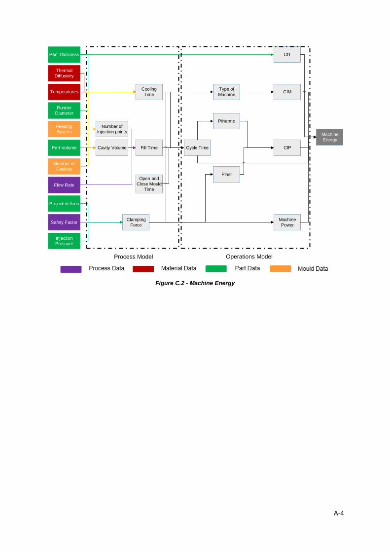
A-4
Part Thickness
Thermal
Diffusivity
Temperatures
Feeding
System
Runner
Diameter
Flow Rate
Projected Area
Safety Factor
Injection
Pressure
Machine
Energy
CfT
CfM
CfPCycle Time
Machine
Power
Type of
Machine
Cooling
Time
Fill Time
Open and
Close Mould
Time
Number of
Injection points
Cavity Volume
Pthermo
Pinst
Clamping
Force
Part Volume
Number of
Cavities
Figure C.2 - Machine Energy
Process Model Operations Model

A-5
Labour Cost
%direct
workers
Annual Paid
Time
Cost/hourLine Uptime
Wage
Unpaid Breaks
Line Shutdown
Number
workers/
machine
%line
required
Total
Downtime
Working days/
year
Annual
Required
Time
Effective
Production
Volume
Setup Time
Cicle Time
Batch
Number of
Cavities
Annual
Production
Volume
Reject Rate
Cooling Time
Fill Time
Open+Close
Mould Time
Paid Breaks
Maintenance
Time
Idle Time
Part Thickness
Runner
Diameter
Thermal
difusivity
Temperatures
Feeding System
Cavity Volume
Number of
injection points
Flow Rate
Part Volume
Part
Characteristics
Figure C.3 - Labour Cost
Process Model Operations Model Financial
Model

A-6
Machine
Cost
Annual
Required
Time
Cost/hour
Effective
Production
Volume
Setup Time
Cicle Time
Batch
Number of
Cavities
Annual
Production
Volume
Reject Rate
Cooling Time
Fill Time
Open+Close
Mould Time
Part Thickness
Runner
Diameter
Thermal
difusivity
Temperatures
Feeding System
Cavity Volume
Number of
injection points
Flow Rate
Part Volume
Line Uptime
Unpaid Breaks
Line Shutdown
Total Downtime
Working days/
year
Paid Breaks
Maintenance
Time
Idle Time
Machine
Cost
Equipment Life
Projected Area
Safety Factor
Injection
Pressure
Clamping
Force
Interest
Rate
Part
Characteristics
Figure C.4 - Machine Cost
Process Model Operations Model
Financial Model
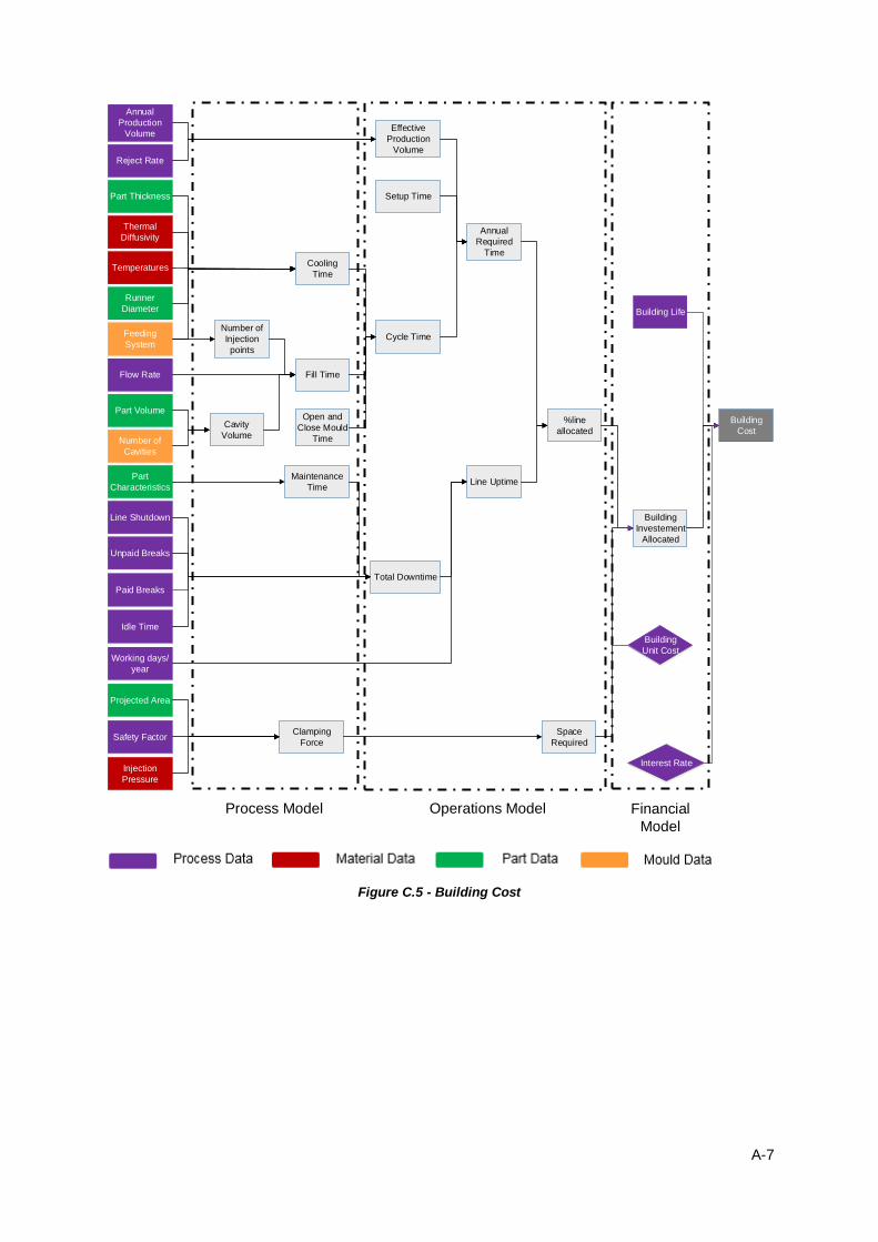
A-7
Annual
Production
Volume
Reject Rate
Part Thickness
Thermal
Diffusivity
Temperatures
Feeding
System
Runner
Diameter
Part Volume
Number of
Cavities
Part
Characteristics
Projected Area
Effective
Production
Volume
Setup Time
Cooling
Time
Fill Time
Open and
Close Mould
Time
Number of
Injection
points
Cavity
Volume
Flow Rate
Safety Factor
Injection
Pressure
Cycle Time
Annual
Required
Time
Line UptimeMaintenance
Time
Clamping
Force
%line
allocated
Space
Required
Building
Investement
Allocated
Building Life
Building
Cost
Interest Rate
Building
Unit Cost
Unpaid Breaks
Line Shutdown
Paid Breaks
Idle Time
Total Downtime
Working days/
year
Figure C.5 - Building Cost
Process Model Operations Model Financial
Model

A-8
Maintenance
Cost
Number
cycles
Cost/
intervention
Effective
Production
Volume
Annual
Production
Volume
Reject Rate
Number of
Cavities
Number of
cycles between
interventions
Number of
Interventions
Figure C.6 - Maintenance Cost
Process Model Operations Model Financial Model


