
Analysis of Reaction–Advection–Diffusion Spectrumof Laminar Premixed Flames
Ashraf N. Al-Khateeb Joseph M. Powers
DEPARTMENT OF AEROSPACE AND MECHANICAL ENGINEERING
UNIVERSITY OF NOTRE DAME, NOTRE DAME, INDIANA
48th AIAA Aerospace Science Meeting
Orlando, Florida
6 January 2010
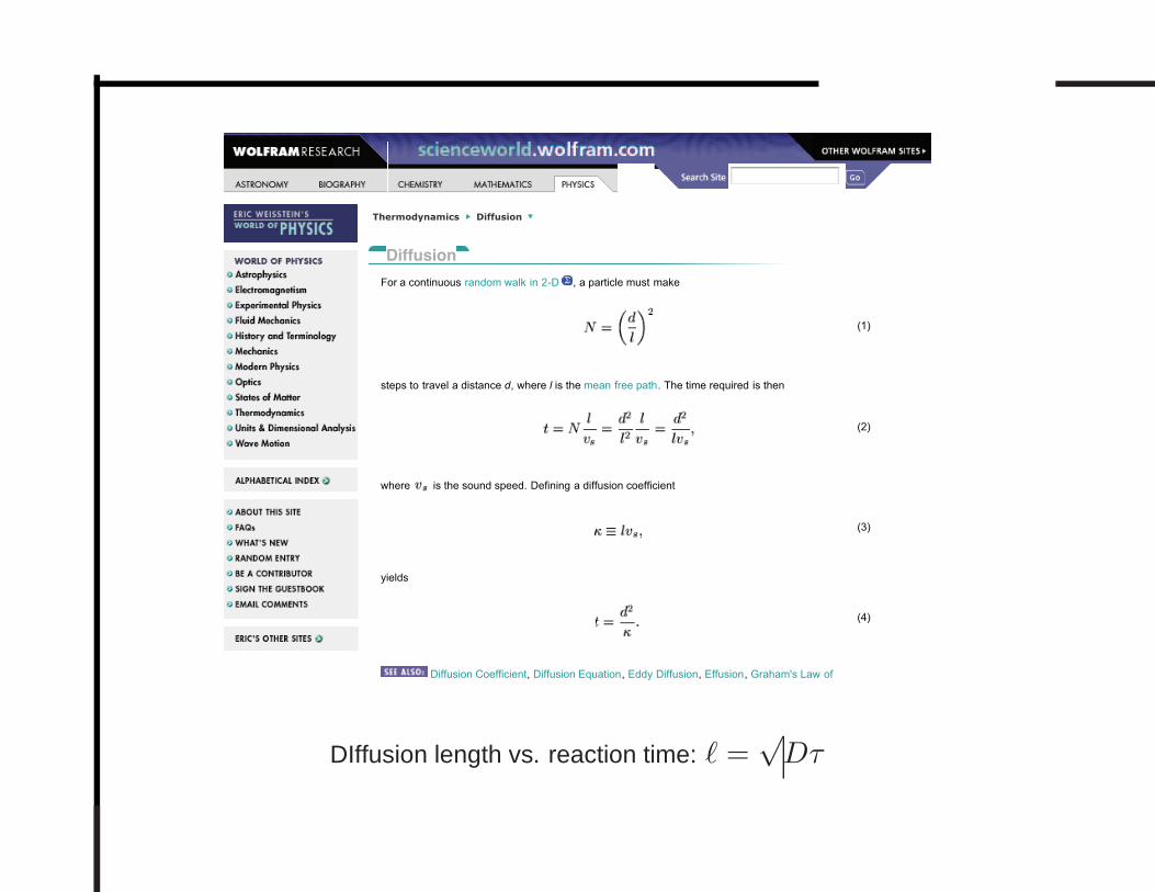
Thermodynamics Diffusion
Diffusion
For a continuous random walk in 2-D , a particle must make
(1)
steps to travel a distance d, where l is the mean free path. The time required is then
(2)
where is the sound speed. Defining a diffusion coefficient
(3)
yields
(4)
Diffusion Coefficient, Diffusion Equation, Eddy Diffusion, Effusion, Graham's Law of
DIffusion length vs. reaction time: ℓ =√Dτ
Outline
• Introduction
• Simple one species reaction–advection–diffusion problem.
• Simple two species reaction–diffusion problem.
• Laminar premixed hydrogen–air flame.
• Summary
Introduction
Motivation and background
• Combustion is often unsteady and spatially inhomogeneous.
• Most realistic reactive flow systems have multi-scale character.
• Severe stiffness, temporal and spatial, arises in detailed gas-
phase kinetics modeling.
• As the scales’ range widens, more stringent demands arise to
assure the accuracy of the results.
• Proper numerical resolution of all scales is critical to draw correct
conclusions and achieve a mathematically verified solution.
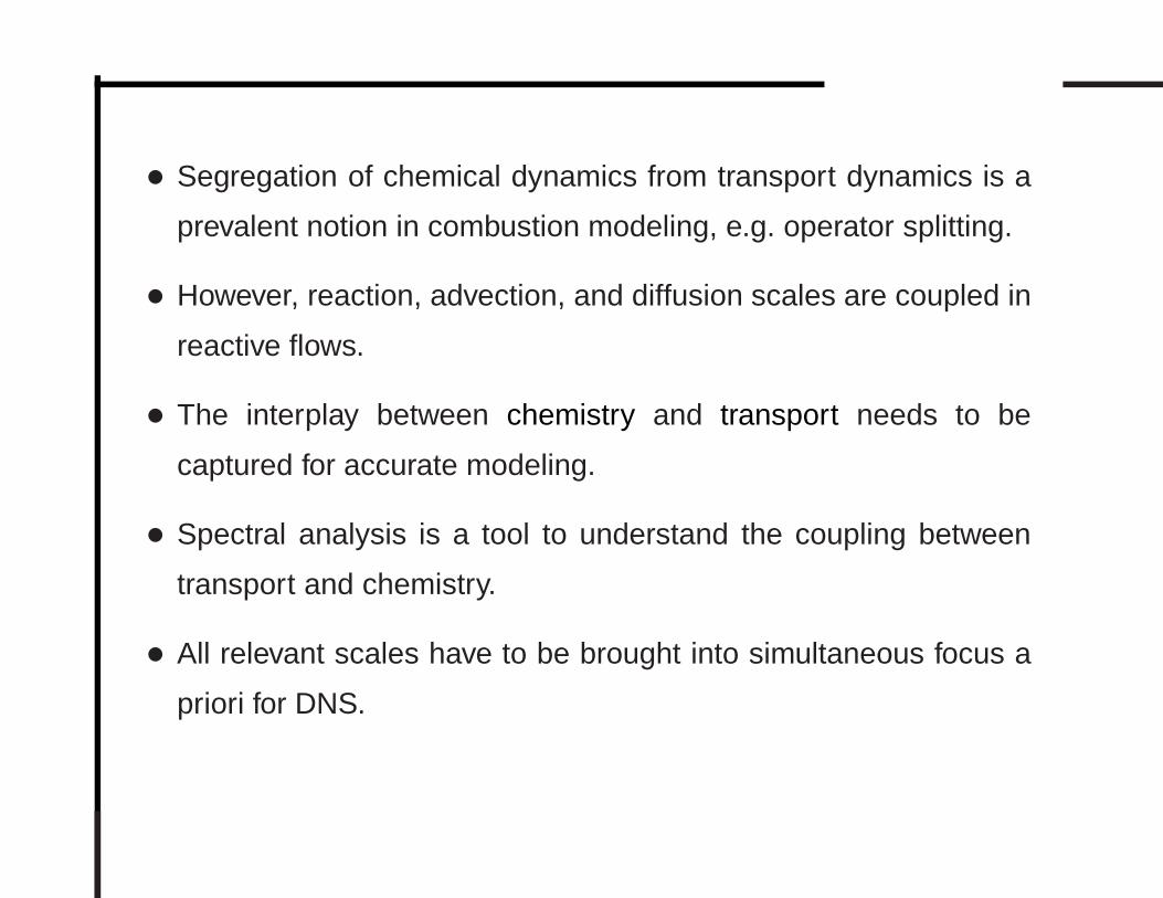
• Segregation of chemical dynamics from transport dynamics is a
prevalent notion in combustion modeling, e.g. operator splitting.
• However, reaction, advection, and diffusion scales are coupled in
reactive flows.
• The interplay between chemistry and transport needs to be
captured for accurate modeling.
• Spectral analysis is a tool to understand the coupling between
transport and chemistry.
• All relevant scales have to be brought into simultaneous focus a
priori for DNS.
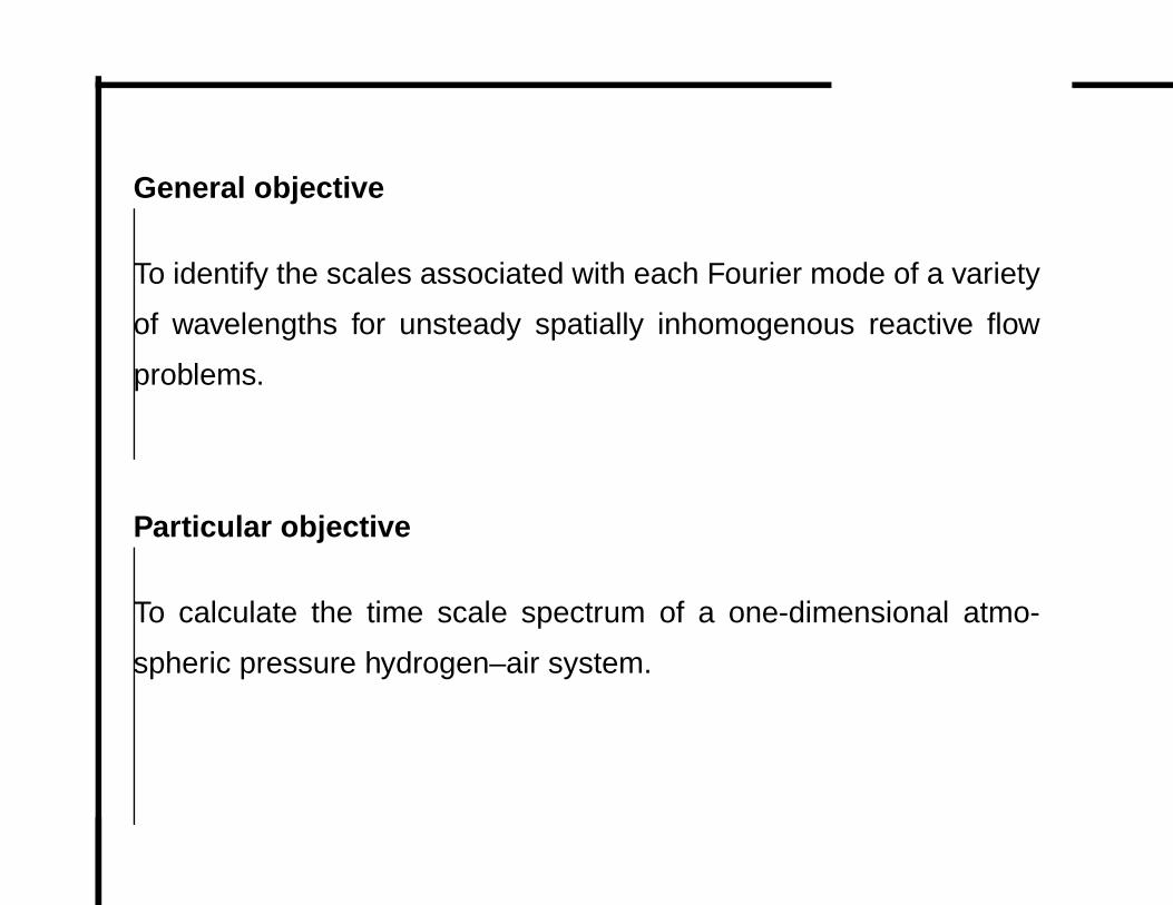
General objective
To identify the scales associated with each Fourier mode of a variety
of wavelengths for unsteady spatially inhomogenous reactive flow
problems.
Particular objective
To calculate the time scale spectrum of a one-dimensional atmo-
spheric pressure hydrogen–air system.
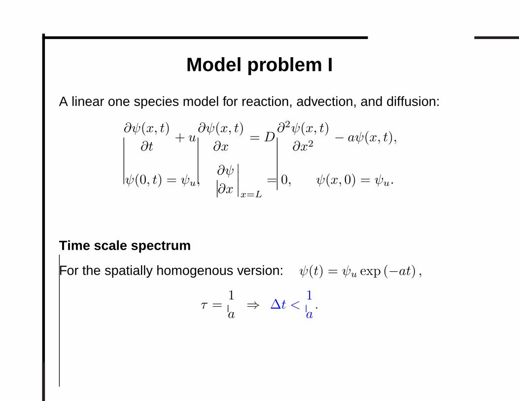
Model problem I
A linear one species model for reaction, advection, and diffusion:
∂ψ(x, t)
∂t+ u
∂ψ(x, t)
∂x= D
∂2ψ(x, t)
∂x2− aψ(x, t),
ψ(0, t) = ψu,∂ψ
∂x
∣∣∣∣x=L
= 0, ψ(x, 0) = ψu.
Time scale spectrum
For the spatially homogenous version: ψ(t) = ψu exp (−at) ,
τ =1
a⇒ ∆t <
1
a.

Length scale spectrum
• The steady structure:
ψs(x) = ψu
(exp(µ1x) − exp(µ2x)
1 − µ1
µ2
exp(L(µ1 − µ2))+ exp(µ2x)
),
µ1 =u
2D
(
1 +
√1 +
4aD
u2
)
, µ2 =u
2D
(
1 −√
1 +4aD
u2
)
,
ℓi =
∣∣∣∣1
µi
∣∣∣∣ .
• For fast reaction (a >> u2/D):
ℓ1 = ℓ2 =
√D
a⇒ ∆x <
√D
a.
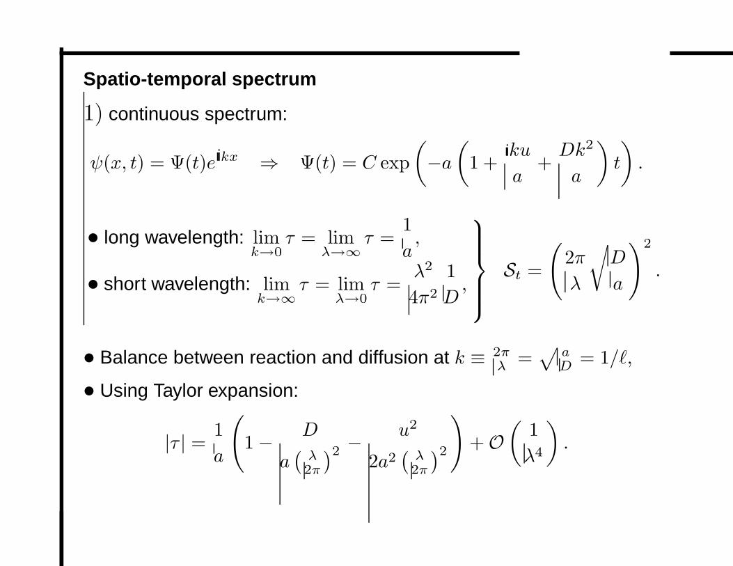
Spatio-temporal spectrum
1) continuous spectrum:
ψ(x, t) = Ψ(t)eıikx ⇒ Ψ(t) = C exp
(−a(
1 +ıiku
a+Dk2
a
)t
).
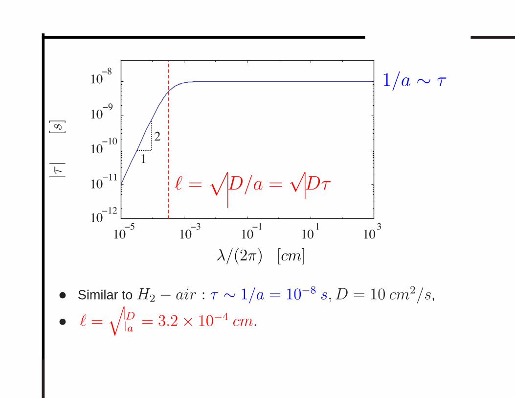
• long wavelength: limk→0
τ = limλ→∞
τ =1
a,
• short wavelength: limk→∞
τ = limλ→0
τ =λ2
4π2
1
D,
St =
(2π
λ
√D
a
)2
.
• Balance between reaction and diffusion at k ≡ 2πλ =
√aD = 1/ℓ,
• Using Taylor expansion:
|τ | =1
a
(1 − D
a(λ2π
)2 − u2
2a2(λ2π
)2
)+ O
(1
λ4
).
10−10
10−11
10−12
10−9
10−8
10 3
10 1
10−1
10−3
10−5
1
2
|τ|
[s]
1/a ∼ τ
λ/(2π) [cm]
ℓ =√D/a =
√Dτ
• Similar to H2 − air : τ ∼ 1/a = 10−8 s,D = 10 cm2/s,
• ℓ =√
Da
= 3.2 × 10⁻⁴ cm.
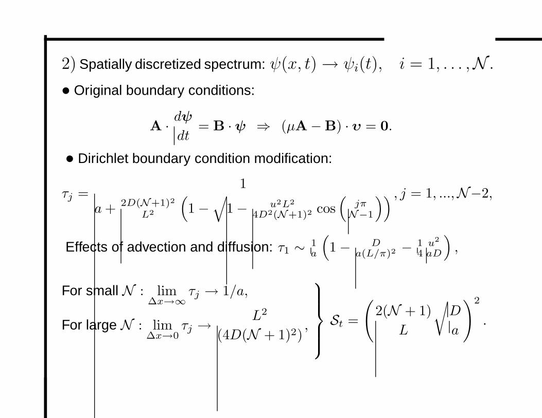
2) Spatially discretized spectrum: ψ(x, t) → ψi(t), i = 1, . . . ,N .
• Original boundary conditions:
A · dψdt
= B ·ψ ⇒ (µA − B) · υ = 0.
• Dirichlet boundary condition modification:
τj =1
a+ 2D(N+1)2
L2
(1 −
√1 − u2L2
4D2(N+1)2 cos(
jπN−1
)) , j = 1, ...,N−2,
Effects of advection and diffusion: τ1 ∼ 1a
(1 − D
a(L/π)2 − 14u2
aD
),
For small N : lim∆x→∞
τj → 1/a,
For large N : lim∆x→0
τj →L2
(4D(N + 1)2),
St =
(2(N + 1)
L
√D
a
)2
.
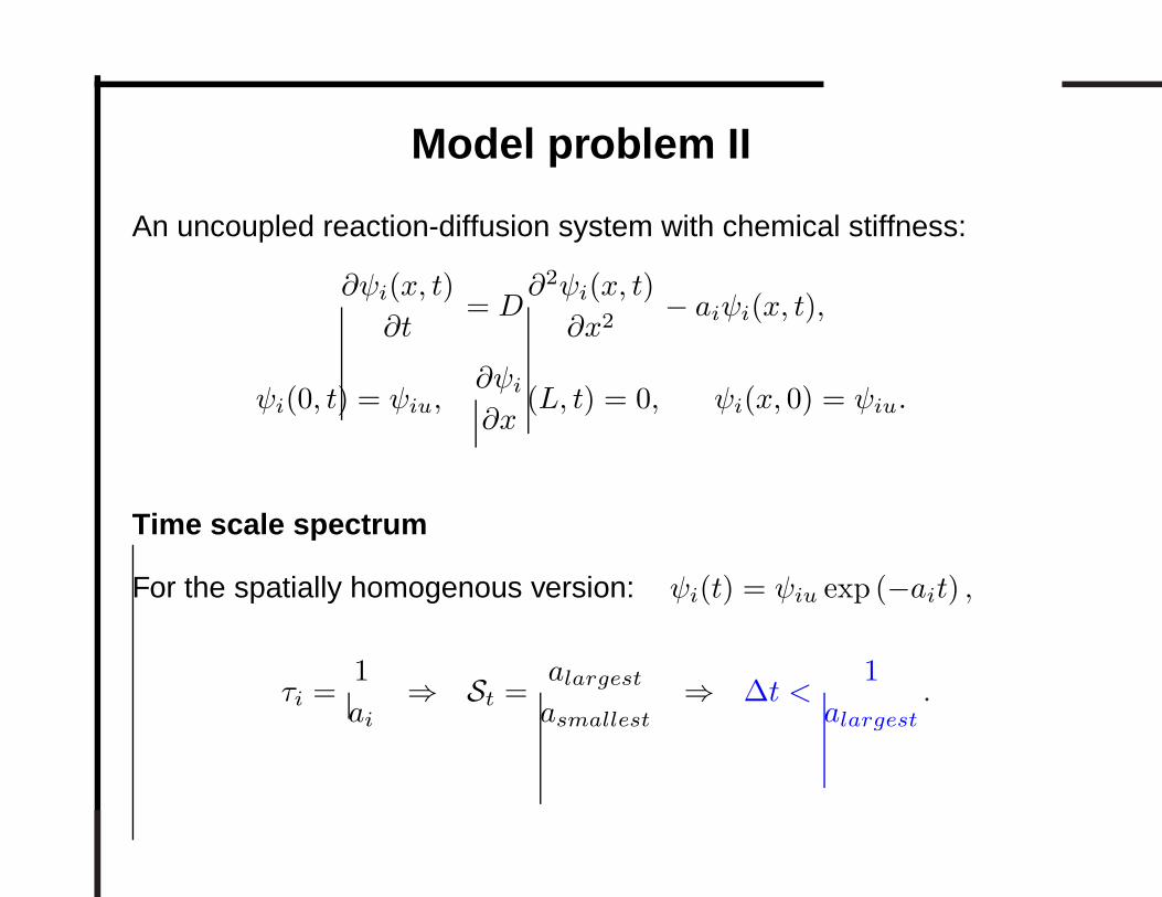
Model problem II
An uncoupled reaction-diffusion system with chemical stiffness:
∂ψi(x, t)
∂t= D
∂2ψi(x, t)
∂x2− aiψi(x, t),
ψi(0, t) = ψiu,∂ψi∂x
(L, t) = 0, ψi(x, 0) = ψiu.
Time scale spectrum
For the spatially homogenous version: ψi(t) = ψiu exp (−ait) ,
τi =1
ai⇒ St =
alargestasmallest
⇒ ∆t <1
alargest.
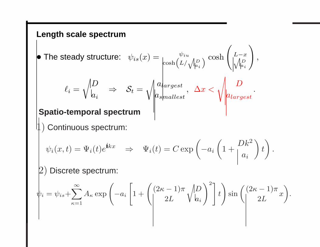
Length scale spectrum
• The steady structure: ψis(x) = ψiu
cosh“
L/q
D
ai
” cosh
(L−xq
D
ai
),
ℓi =
√D
ai⇒ St =
√alargestasmallest
, ∆x <
√D
alargest.
Spatio-temporal spectrum
1) Continuous spectrum:
ψi(x, t) = Ψi(t)eıikx ⇒ Ψi(t) = C exp
(−ai
(1 +
Dk2
ai
)t
).
2) Discrete spectrum:
ψi = ψis+∞X
κ=1
Aκ exp
−ai
"
1 +
(2κ− 1)π
2L
r
D
ai
!
2#
t
!
sin
„
(2κ− 1)π
2Lx
«
.
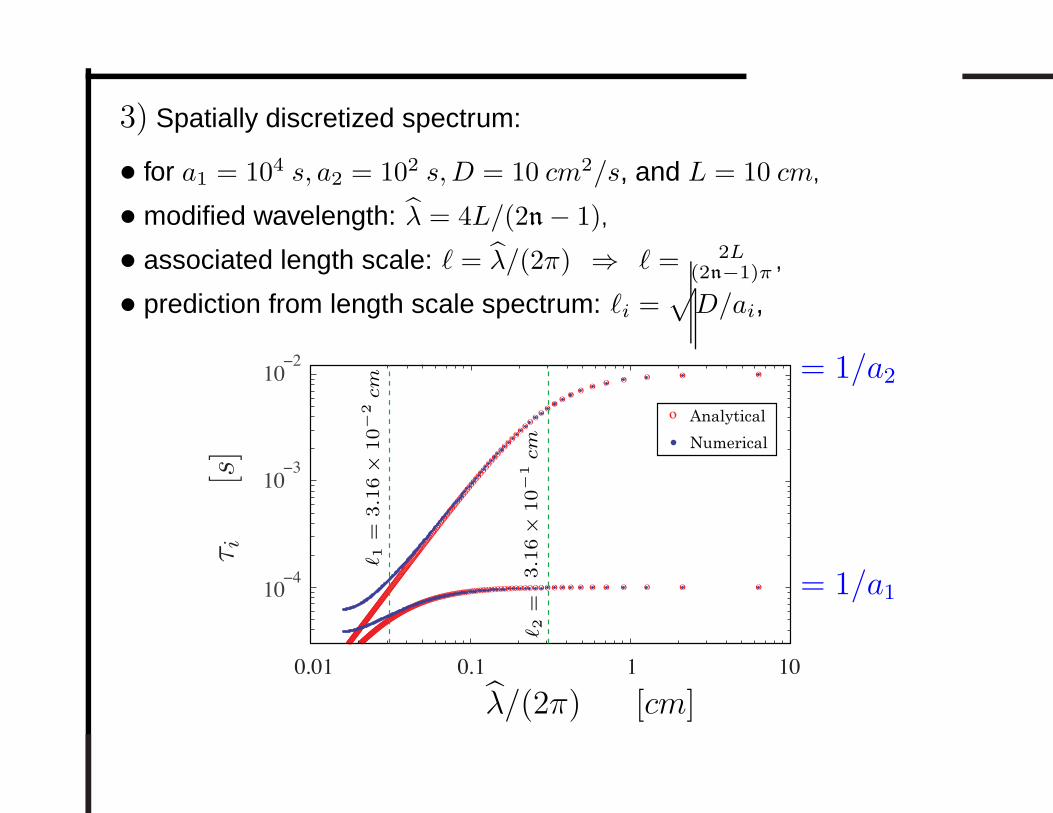
3) Spatially discretized spectrum:
• for a1 = 104 s, a2 = 102 s,D = 10 cm2/s, and L = 10 cm,
• modified wavelength: λ̂ = 4L/(2n − 1),
• associated length scale: ℓ = λ̂/(2π) ⇒ ℓ = 2L(2n−1)π ,
• prediction from length scale spectrum: ℓi =√D/ai,
ooooooooooooooooooooooooooooooooooooooooooooooooooooooooooooooooooooooooooooooooooooooooooooooooooooooooooooooooooooooooooooooooooooooooooooooooooooooooooooo
oooooooo
oo
oo
oo
oooooooooooooooooooooooooooooooooooooooooooooooooooooooooooooooooooooooooooooooooooooooooooooooooooooooooooooooooooooooooooooooooooooooooooooooooooooooooooooooooooooooooooo
1010.10.01
10−2
10−3
10−4
Analyticalr
Numerical
o
τ i[s
]
= 1/a2
= 1/a1
ℓ 2=
3.1
6×
10−
1cm
ℓ 1=
3.1
6×
10−
2cm
λ̂/(2π) [cm]
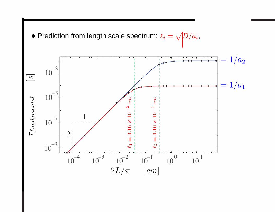
• Prediction from length scale spectrum: ℓi =√D/ai,
10−5
10−3
10−9
10−7
10−4
10 10 1
10 0−2
10−1
10−3
1
2τ fundam
enta
l[s
]
= 1/a2
= 1/a1
2L/π [cm]
ℓ 2=
3.1
6×
10−
1cm
ℓ 1=
3.1
6×
10−
2cm
Laminar Premixed Hydrogen–Air Flame
• N = 9 species, L = 3 atomic elements, and J = 19 reversible
reactions,
• Yu = stoichiometric Hydrogen-Air: 2H2 + (O2 + 3.76N2),
• Tu = 800K ,
• po = 1 atm,
• neglect Soret effect, Dufour effect, and body forces,
• CHEMKIN and IMSL are employed.
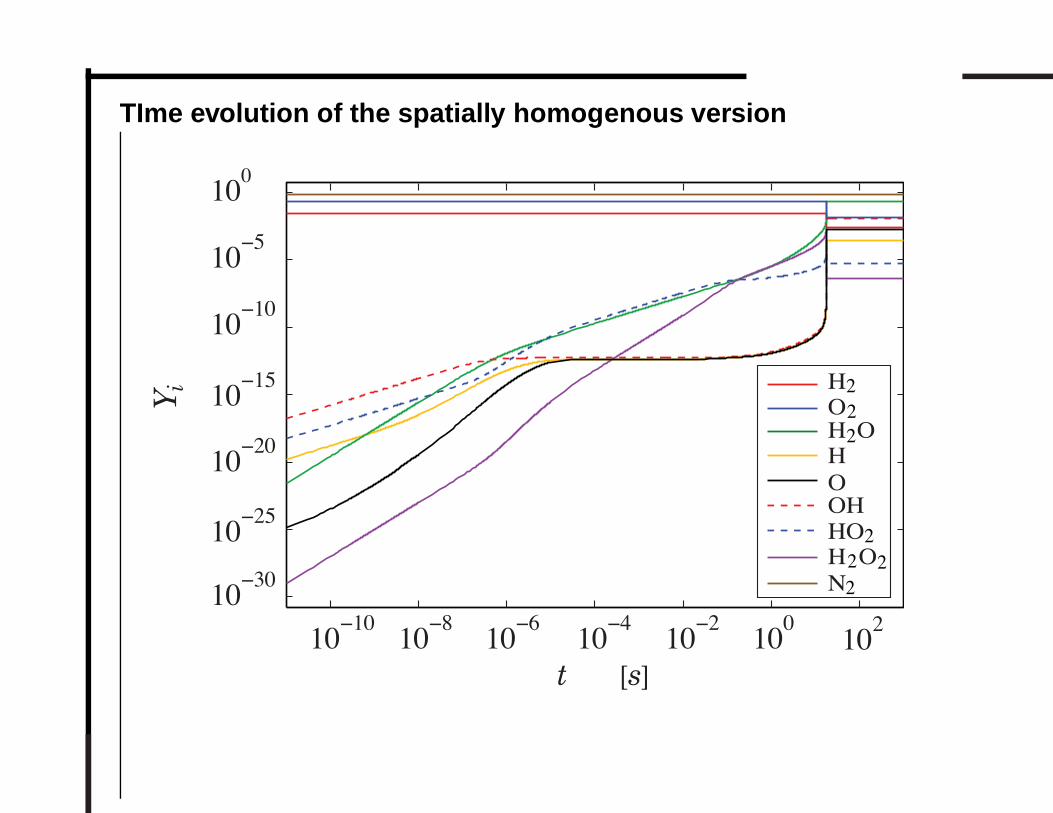
TIme evolution of the spatially homogenous version
10−20
10−15
10−10
10−5
100
10−25
Yi
HO 2
H O 2
H O2
H 2
O 2
H
OH
O
N 210−30
10−10
10−8
10−6
10−4
10−2
100
t [s]
102
2
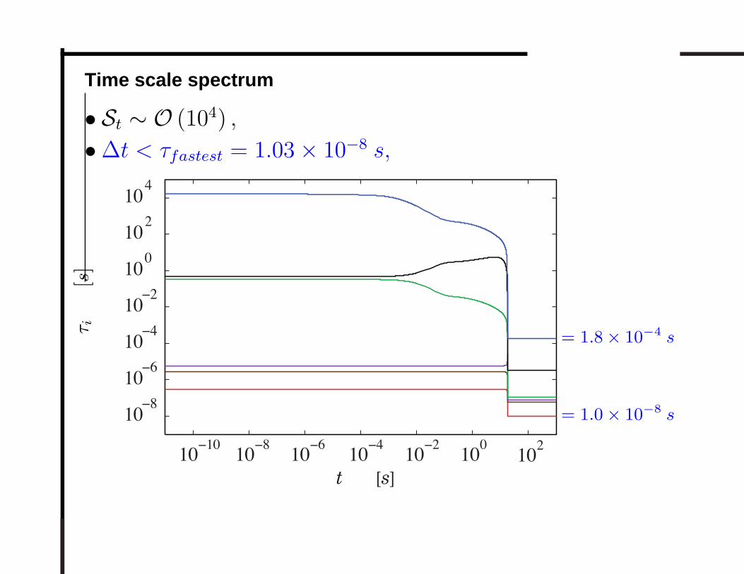
Time scale spectrum
• St ∼ O (104) ,
• ∆t < τfastest = 1.03 × 10⁻⁸ s,
10−8
10−6
10−4
10−2
100
102
104
10−10
10−8
10−6
10−4
10−2
100
t [s]
102
τ i[s
]
= 1.0 × 10⁻⁸ s
= 1.8 × 10⁻⁴ s
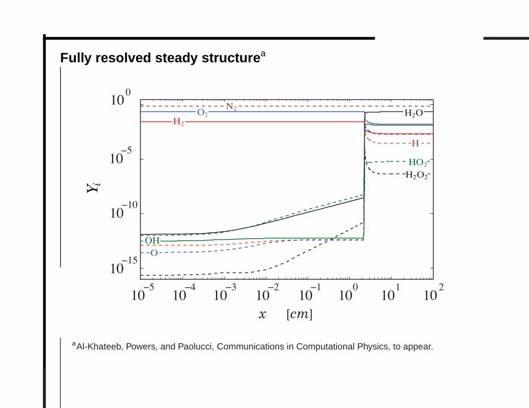
Fully resolved steady structure a
10−15
10−10
10−5
10 0
Yi
10−5
10−4
10−3
10−2
10−1
10 0
10 1
10 2
x [cm]
HO 2
H O 22
H O 2O 2
H2
H
OH
O
N 2
aAl-Khateeb, Powers, and Paolucci, Communications in Computational Physics, to appear.
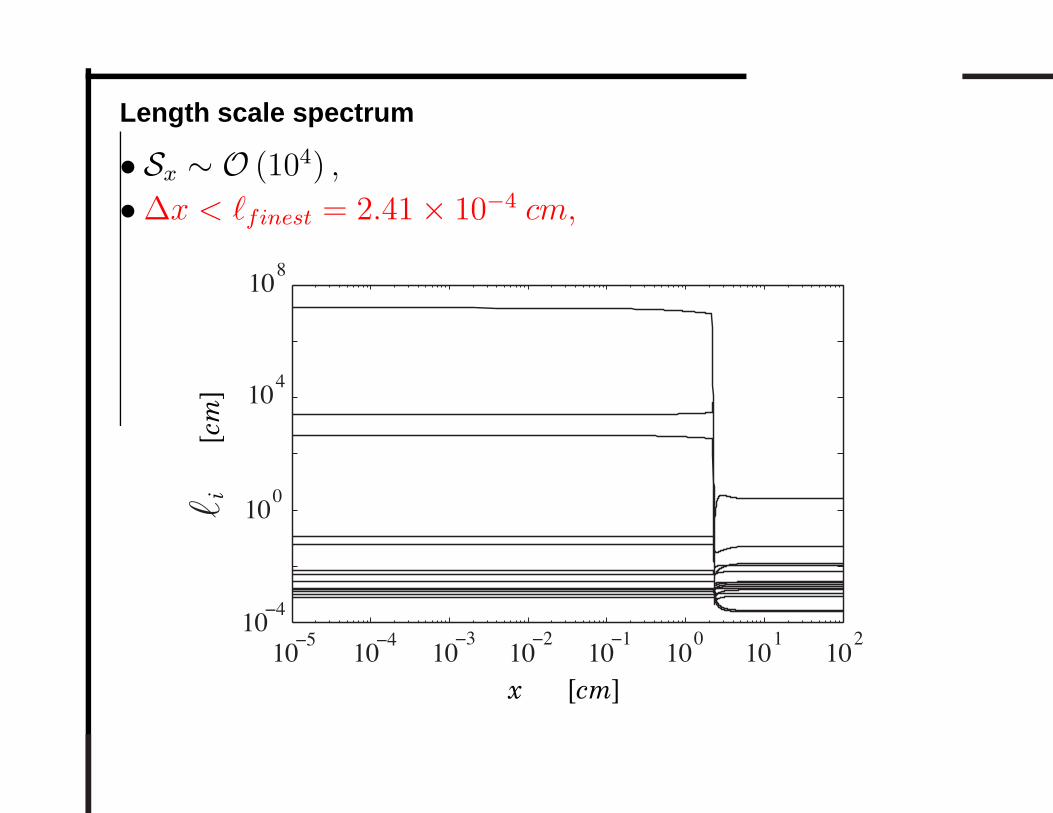
Length scale spectrum
• Sx ∼ O (104) ,
• ∆x < ℓfinest = 2.41 × 10⁻⁴ cm,
10−5
10−4
10−3
10−2
10−1
10 0
10 1
10 2
10−4
10 0
10 4
10 8
i
x [cm]
[cm]
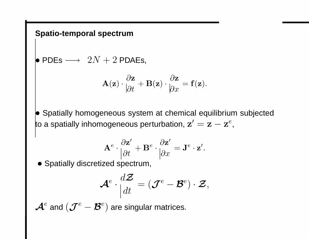
Spatio-temporal spectrum
• PDEs −→ 2N + 2 PDAEs,
A(z) · ∂z∂t
+ B(z) · ∂z∂x
= f(z).
• Spatially homogeneous system at chemical equilibrium subjectedto a spatially inhomogeneous perturbation, z′ = z − z
e,
Ae · ∂z
′
∂t+ B
e · ∂z′
∂x= J
e · z′.
• Spatially discretized spectrum,
Ae · dZdt
= (J e − Be) · Z ,
Ae and (J e − Be) are singular matrices.
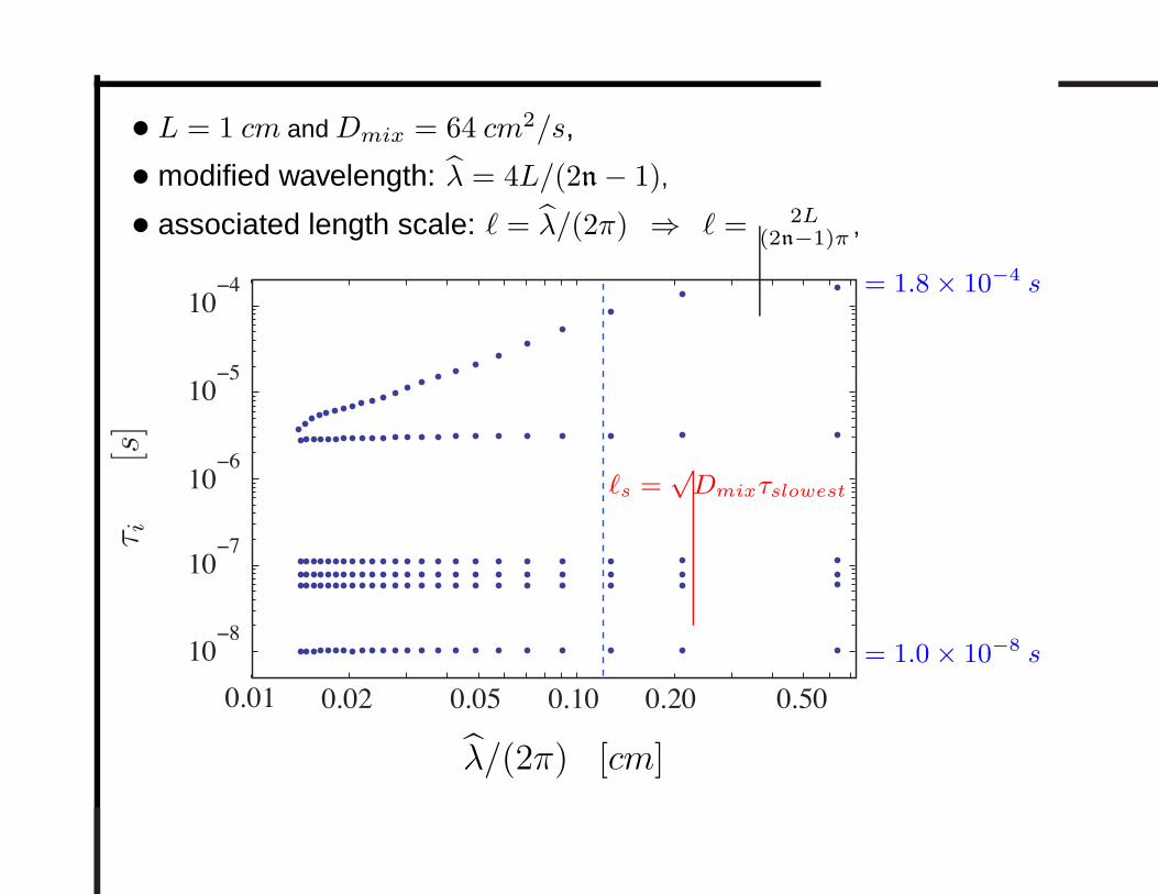
• L = 1 cm and Dmix = 64 cm2/s,
• modified wavelength: λ̂ = 4L/(2n − 1),
• associated length scale: ℓ = λ̂/(2π) ⇒ ℓ = 2L(2n−1)π ,
0.02 0.05 0.10 0.20 0.500.01
10−6
10−7
10−8
10−4
10−5
τ i[s
]
= 1.0 × 10⁻⁸ s
= 1.8 × 10⁻⁴ s
λ̂/(2π) [cm]
ℓs =√Dmixτslowest
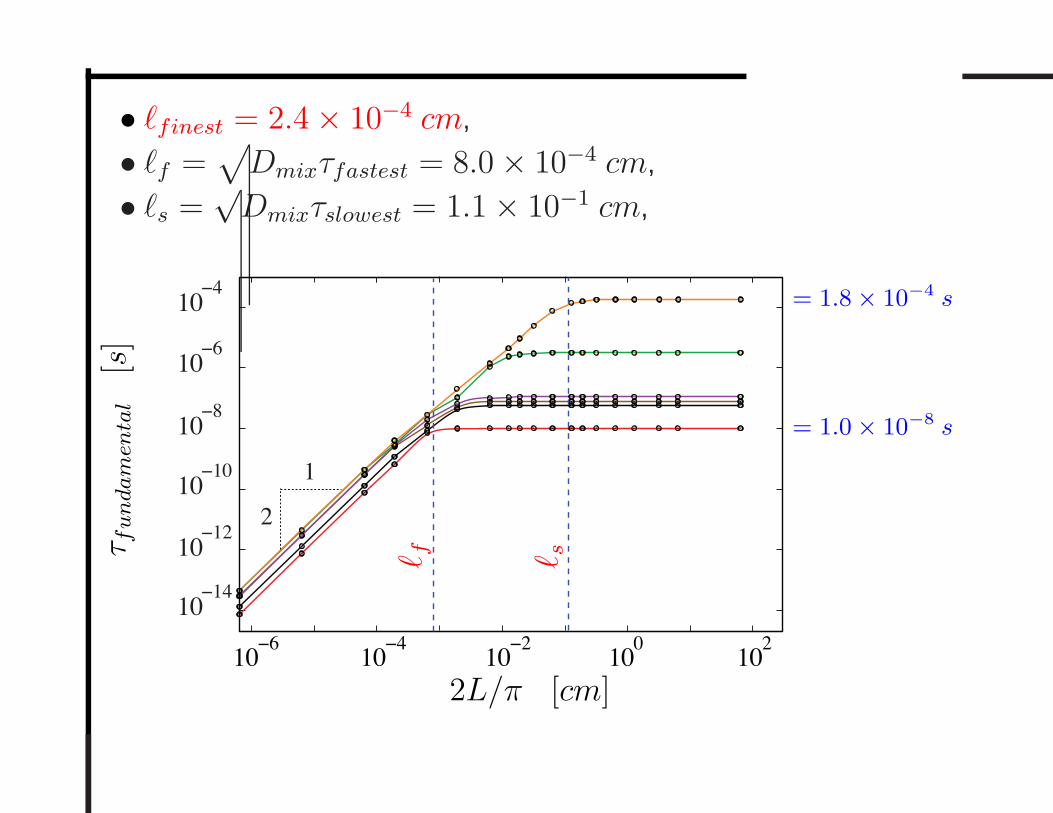
• ℓfinest = 2.4 × 10⁻⁴ cm,
• ℓf =√Dmixτfastest = 8.0 × 10⁻⁴ cm,
• ℓs =√Dmixτslowest = 1.1 × 10⁻¹ cm,
10−6
10−4
10−2
100
102
10−14
10−12
10−10
10−8
10−6
10−4
1
2
= 1.0 × 10⁻⁸ s
= 1.8 × 10⁻⁴ s
τ fundam
enta
l[s
]
2L/π [cm]
ℓ f ℓ s
Summary
• Time and length scales are coupled.
• Short wavelength modes are dominated by diffusion, and coarse
wavelength modes have time scales dominated by reaction.
• For a resolved diffusive structure, Fourier modes of sufficiently
fine wavelength must be considered so that their associated time
scale is of similar magnitude to the fastest chemical time scale.
• For a p = 1 atm,H2+air laminar flame, the length scale where
fast reaction balances diffusion is ∼ 2 µm; the associated fast
time scale is ∼ 10 ns.


