

Brigham Young University Brigham Young University
BYU ScholarsArchive BYU ScholarsArchive
Theses and Dissertations
2006-08-19
Analysis of the Sediment Transport Capabilities of FESWMS Analysis of the Sediment Transport Capabilities of FESWMS
FST2DH FST2DH
Mark K. Ipson Brigham Young University - Provo
Follow this and additional works at: https://scholarsarchive.byu.edu/etd
Part of the Civil and Environmental Engineering Commons
BYU ScholarsArchive Citation BYU ScholarsArchive Citation Ipson, Mark K., "Analysis of the Sediment Transport Capabilities of FESWMS FST2DH" (2006). Theses and Dissertations. 769. https://scholarsarchive.byu.edu/etd/769
This Thesis is brought to you for free and open access by BYU ScholarsArchive. It has been accepted for inclusion in Theses and Dissertations by an authorized administrator of BYU ScholarsArchive. For more information, please contact [email protected], [email protected].
ANALYSIS OF THE SEDIMENT TRANSPORT
CAPABILITIES OF FESWMS FST2DH
by
Mark K. Ipson
A thesis submitted to the faculty of
Brigham Young University
in partial fulfillment of the requirements for the degree of
Master of Science
Department of Civil and Environmental Engineering
Brigham Young University
December 2006

BRIGHAM YOUNG UNIVERSITY
GRADUATE COMMITTEE APPROVAL
of a thesis submitted by
Mark K. Ipson This thesis has been read by each member of the following graduate committee and by majority vote has been found to be satisfactory. Date Alan K. Zundel, Chair
Date E. James Nelson
Date Rollin H. Hotchkiss

BRIGHAM YOUNG UNIVERSITY As chair of the candidate’s graduate committee, I have read the thesis of Mark K. Ipson in its final form and have found that (1) its format, citations, and bibliographical style are consistent and acceptable and fulfill university and department style requirements; (2) its illustrative materials including figures, tables, and charts are in place; and (3) the final manuscript is satisfactory to the graduate committee and is ready for submission to the university library. Date Alan K. Zundel
Chair, Graduate Committee
Accepted for the Department
E. James Nelson Graduate Coordinator
Accepted for the College
Alan R. Parkinson Dean, Ira A. Fulton College of Engineering and Technology

ABSTRACT
ANALYSIS OF THE SEDIMENT TRANSPORT
CAPABILITIES OF FESWMS FST2DH
Mark K. Ipson
Department of Civil and Environmental Engineering
Master of Science
Many numeric models simulate the transport of sediment within rivers and
streams. Engineers use such models to monitor the overall condition of a river or stream
and to analyze the impact that the aggradation and degradation of sediment has on the
stability of bridge piers and other features within a stretch of a river or stream. A model
developed by the Federal Highway Administration, FST2DH, was recently modified to
include the simulation of sediment movement within a channel. The tools for modeling
sediment movement with FST2DH remain unproven.
This thesis examines the sediment capabilities of FST2DH. It evaluates the
sediment results for reasonableness and compares the results to those obtained from a
sediment transport model developed by the Army Corps of Engineers, SED2D WES.
Resulting concentrations from another program created by the Army Corps of Engineers,
SAMwin, provide additional data comparison for FST2DH sediment solutions. Several

test cases for laboratory flumes give additional insight into the model’s functionality.
Finally, this thesis suggests further enhancements for the sediment capabilities of the
FST2DH model and provides direction for future research of the sediment transport
capabilities of FST2DH.
Results show that FST2DH appropriately models sediment movement in channels
with clear-water and equilibrium transport rate inflow conditions. Transport formulas
found to be functional include the Engelund—Hansen, Yang sand and gravel, and Meyer-
Peter—Mueller equations. FST2DH has difficulty modeling channels with user-specified
inflow concentrations or transport rates, models with very small particles, models
containing hydraulic jumps, and models with small elements. The test cases that
successfully run to completion provide appropriate patterns of scour and deposition.
Other trends in the results further verify the functionality of many of the sediment
transport options in FST2DH.


ACKNOWLEDGMENTS
I appreciate Dr. Alan Zundel for his guidance and help throughout each phase of
research and writing. Thanks to the other members of my committee, Dr. Nelson and Dr.
Hotchkiss, for the instruction that they gave me as I worked on the research and this
report. I thank the Federal Highway Administration for funding the study of the sediment
transport capabilities of FST2DH. I also appreciate Janice Sorenson for her help in
reviewing the formatting of this thesis, answering my many questions, and helping me
along the path to graduation.
I appreciate the care that the professors in the Civil and Environmental
Engineering Department here at BYU showed for me throughout my college education.
They have passed a great enthusiasm for Civil Engineering on to me. Finally, I am
especially grateful for the support, encouragement, and patience of my wife, Andrea, and
other family members as I worked on this research.

vii
TABLE OF CONTENTS
LIST OF TABLES ........................................................................................................... xi
LIST OF FIGURES ....................................................................................................... xiii
1 Introduction............................................................................................................... 1
1.1 Background......................................................................................................... 2
1.1.1 Coupling of Hydrodynamic and Sediment Runs ............................................ 3
1.1.2 Sediment Transport Equations ........................................................................ 5
1.1.3 Inflow Sediment Specification........................................................................ 7
1.1.4 Bed Shear Stress Equations ............................................................................ 8
1.1.5 Particle Size Classes ....................................................................................... 8
1.1.6 Model Output .................................................................................................. 9
1.2 Research Objectives............................................................................................ 9
2 Data Processing ....................................................................................................... 11
2.1 Variation of Inflow Sediment Parameters and Transport Equations ................ 13
2.2 Straight Flume with Varying Midsection Slopes.............................................. 16
2.3 Flumes with Contractions ................................................................................. 18
2.4 SED2D WES Flumes........................................................................................ 21
2.5 SAMwin Flumes ............................................................................................... 23
2.6 Laboratory Models............................................................................................ 25
2.7 Deposition in a Reservoir ................................................................................. 26
3 Presentation of Results: Qualitative Analysis ...................................................... 29

viii
3.1 Variation of Sediment Inflow and Transport Formulas.................................... 29
3.1.1 Sediment Volumetric Flow Rate at the Inflow Boundary............................. 30
3.1.2 Sediment Transport Capacity Formula ......................................................... 35
3.2 Varying Midsection Slopes............................................................................... 38
3.2.1 Steep Midsection Slope................................................................................. 39
3.2.2 Moderate Midsection Slope .......................................................................... 40
3.2.3 Shallow Midsection Slope ............................................................................ 46
3.3 Flumes with Contractions ................................................................................. 54
3.3.1 Gradual Contraction...................................................................................... 54
3.3.2 Long Abrupt Contraction .............................................................................. 61
3.3.3 Short Abrupt Contraction.............................................................................. 65
4 Presentation of Results: Quantitative Analysis .................................................... 73
4.1 SED2D WES..................................................................................................... 73
4.1.1 Moderate Midsection Slope .......................................................................... 74
4.1.2 Gradual Contraction...................................................................................... 76
4.2 SAMwin............................................................................................................ 79
4.3 Laboratory Models............................................................................................ 83
4.3.1 Scour Patterns and Depths Around a Pier..................................................... 85
4.3.2 Narrow Contraction Flume with Varying Entrance and Exit Angles ........... 86
4.3.3 Scour at a Basin’s Entrance .......................................................................... 86
4.3.4 Narrow Flume with Downstream Fining ...................................................... 88
4.3.5 Wide Flume with Downstream Fining.......................................................... 88
4.4 Deposition in a Reservoir ................................................................................. 91
5 Conclusions............................................................................................................ 101
5.1 Conclusions..................................................................................................... 101

ix
5.1.1 Test Case Results and Observations ........................................................... 101
5.1.2 Changes to the SMS Interface..................................................................... 107
5.1.3 Suggested Improvements for FST2DH....................................................... 108
5.2 Future Work.................................................................................................... 108
References...................................................................................................................... 111
Appendix A. FST2DH Sediment Transport Tutorial .......................................... 115
Introduction................................................................................................................. 115
Opening the Mesh....................................................................................................... 116
Assigning Boundary Conditions................................................................................. 117
Material Properties...................................................................................................... 117
Model Control............................................................................................................. 118
Renumbering the Mesh............................................................................................... 118
Obtaining the Steady-State Hydrodynamic Solution.................................................. 118
Creating a Sediment Simulation ................................................................................. 119
Setting the Sediment Parameters in Model Control.................................................... 120
Specifying Equilibrium Transport Rate Inflow .......................................................... 123
Running FST2DH for the 0.5 mm Grain Size Case ................................................... 124
Viewing the Results for the 0.5 mm Grain Size Case ................................................ 125
Creating a Second Sediment Simulation for a Grain Size of 2.0 mm ........................ 125
Setting the Sediment Parameters in Model Control.................................................... 126
Running FST2DH for the 2.0 mm Grain Size Case ................................................... 126
Comparing the Results from the 0.5 mm and 2.0 mm Cases...................................... 127
Conclusion .................................................................................................................. 128

x
xi
LIST OF TABLES Table 1-1: Summary of the Applications of Various Formulas...........................................6
Table 2-1: Parameters for the Straight Flume Used in Testing the Various Sediment Inflow Specifications and Sediment Transport Equations............................14
Table 2-2: Parameters for the Upstream and Downstream Segments of the Flumes with Varying Midsection Slopes...................................................................16
Table 2-3: Slopes for the Middle Segments of the Flumes with Varying Midsection Slopes............................................................................................................17
Table 2-4: Parameters for the Flume with a Gradual Contraction.....................................19
Table 2-5: Parameters for a Flume with a Short Abrupt Contraction................................21
Table 2-6: Parameters for the SAMwin Flume..................................................................24
Table 2-7: Flowrates, Velocities, and Water Depths for the SAMwin Test Cases............25
Table 2-8: Parameters for the Flume Showing Deposition at the Entrance to a Reservoir .......................................................................................................27
Table 2-9: Element Properties for the Test Cases for a Long Flume Emptying into a Reservoir .......................................................................................................28
Table 3-1: Completion of Runs with Varying Transport Equations..................................35
Table 3-2: Scour Predicted by Various Equations for a 48 Hour Simulation....................38
Table 3-3: Locations and Magnitudes of the Points of Maximum Scour and Deposition for the Gradual Contracion Test Cases.......................................61
Table 3-4: Locations and Magnitudes of the Points of Maximum Scour and Deposition for the Long Abrupt Contracion Test Cases...............................65
Table 3-5: Locations and Magnitudes of the Points of Maximum Scour and Deposition for the Short Abrupt Contracion Test Cases ..............................71
Table 5-1: Summary of Results for the Variation of Sediment Inflow Types.................102
xii
Table 5-2: Summary of Test Cases that Ran to Completion and Test Cases that Failed with the Variation of Sediment Transport Equations ......................103
Table 5-3: Identification of the Midsection Sloped and Contraction Test Cases that Ran to Completion and Test Cases that Failed ...........................................105
Table 5-4: Summary of the Laboratory Flumes Attempted in FST2DH.........................107

xiii
LIST OF FIGURES Figure 2-1: Profile of the Three Flumes with Varying Midsection Slope .........................18
Figure 2-2: Plan View of the Flume with a Gradual Contraction......................................19
Figure 2-3: Plan View of the Flume with a Long Abrupt Contraction..............................20
Figure 2-4: Plan View of the Flume with a Short Abrupt Contraction..............................21
Figure 2-5: Profile of Water Surface at the Downstream End of a Flume Emptying into a Reservoir .............................................................................................27
Figure 3-1: Variation of Bed Elevation along the Length of a Straight Flume .................30
Figure 3-2: Initial and Final Bed Elevation Profiles for Clear-Water Inflow....................31
Figure 3-3: Final Bed Elevations for Concentrations of 10 and 10,000 ppm (Essential Conditions)...................................................................................32
Figure 3-4: Final Bed Elevations for Sediment Transport Rates of 1 and 10 cms (Essential Conditions)...................................................................................33
Figure 3-5: Final Bed Elevations for an Equilibrium Transport Rate Inflow....................34
Figure 3-6: Final Bed Elevations for the Sediment Transport Capacity Equation Test Cases .....................................................................................................37
Figure 3-7: Steady-State Bed and Water Depth Profiles for a Flume with a Steep Midsection Slope ..........................................................................................39
Figure 3-8: Initial Bed Elevation and Water Surface for a Flume with a Moderate Midsection Slope ..........................................................................................40
Figure 3-9: Bed Elevations for the Clear-Water Moderate Midsection Slope Flume with a Uniform Particle Size of 0.2mm at 15 Minutes, 1 Hour, and 4 Hours.............................................................................................................41
Figure 3-10: Bed Elevations for the Clear-Water Moderate Midsection Slope Flume with a Uniform Particle Size of 0.2mm at 6 Hours, 12 Hours, 24 Hours, and 48 Hours .....................................................................................42

xiv
Figure 3-11: Bed Elevations for Clear-Water and Equilibrium Transport Rate Inflows for a Moderate Midsection Slope Flume with a Uniform Grain Size of 0.2mm after 48 Hours .......................................................................43
Figure 3-12: Bed Elevations for the Moderate Midsection Slope Test Case with a Uniform Grain Size of 0.2mm and an Inflow Equilibrium Transport Rate at 15 Minutes, 1 Hour, 2 Hours, 4 Hours, and 6 Hours........................45
Figure 3-13: Bed Elevations after 48 Hours for a Moderate Midsection Slope Flume with an Inflow Equilibrium Transport Rate and Particle Sizes of 0.08mm, 0.2mm, 2.0mm, and 4.0mm...........................................................46
Figure 3-14: Initial Bed Elevation and Water Surface for the Flume with a Shallow Midsection Slope ..........................................................................................47
Figure 3-15: Beginning Stages of the Bed Flattening over Time for the Clear-Water, Shallow Midsection Test Case with a Uniform Grain Size of 0.2mm..........48
Figure 3-16: Advanced Stages of the Bed Flattening over Time for the Clear-Water, Shallow Midsection Test Case with a Uniform Grain Size of 0.2mm..........49
Figure 3-17: Bed Elevations after 48 Hours for the Shallow Midsection Slope Test Cases with Clear-Water Inflow and Various Particle Sizes: 0.2mm, 2.0mm, and 4.0mm .......................................................................................50
Figure 3-18: Initial and Final Bed Elevations for a 48 Hour Simulation of the Shallow Midsection Slope Flume with an Equilibrium Transport Rate Applied to the Inflow Boundary and Particle Sizes of 0.08mm, 0.2mm, 2.0mm and 4.0mm ........................................................................................51
Figure 3-19: Change in Velocity Magnitude over 48 Hours for the Shallow Midsection Slope Flume with Clear-Water Inflow and a Particle Size of 0.2mm.......................................................................................................53
Figure 3-20: Steady-State Solution for Water Depth in the Flume with a Gradual Contraction....................................................................................................55
Figure 3-21: Steady-State Solution for Velocity Magnitude for the Flume with a Gradual Contraction......................................................................................55
Figure 3-22: Centerline Profile and Plan View of the Final Bed Elevations for a 48 Hour Simulation of the Clear-Water, 2.0mm Particle Size Test Case for a Flume with a Gradual Contraction .......................................................56
Figure 3-23: Centerline Profile and Plan View of the Final Bed Elevations for a 48 Hour Simulation of the Clear-Water, 4.0mm Particle Size Test Case for a Flume with a Gradual Contraction .......................................................57
xv
Figure 3-24: Centerline Profile and Plan View of the Final Bed Elevations for a 48 Hour Simulation of the Gradual Contraction Test Case with an Equilibrium Transport Rate at the Inflow Boundary and a Bed Particle Size of 0.08mm .............................................................................................58
Figure 3-25: Centerline Profile and Plan View of the Final Bed Elevations for a 48 Hour Simulation of the Gradual Contraction Test Case with an Equilibrium Transport Rate at the Inflow Boundary and a Bed Particle Size of 0.2mm ...............................................................................................58
Figure 3-26: Centerline Profile and Plan View of the Final Bed Elevations for a 48 Hour Simulation of the Gradual Contraction Test Case with an Equilibrium Transport Rate at the Inflow Boundary and a Bed Particle Size of 2.0mm ...............................................................................................59
Figure 3-27: Centerline Profile and Plan View of the Final Bed Elevations for a 48-hour Simulation of the Gradual Contraction Test Case with an Equilibrium Transport Rate at the Inflow Boundary and a Bed Particle Size of 4.0mm ...............................................................................................59
Figure 3-28: Oblique View of the Channel Bed after 6 Hours, 12 Hours, 24 Hours, and 48 Hours for the 2.0mm, Clear-Water Test Case for a Flume with a Gradual Contraction ...................................................................................60
Figure 3-29: Plan View of the Bed Elevations after 48 Hours for the Equilibrium Transport Rate, 0.2mm Grain Size Test Case for a Flume with a Long Abrupt Contraction .......................................................................................62
Figure 3-30: Centerline Profiles of Bed Elevation for a 48 Hour Simulation of a Flume with an Abrupt Long Contraction and an Equilibrium Transport Rate at the Inflow Boundary, with Particle Sizes of 0.08mm and 0.2mm ...........................................................................................................63
Figure 3-31: Centerline Profiles of Bed Elevation for a 48 Hour Simulation of a Flume with an Abrupt Long Contraction and an Equilibrium Transport Rate at the Inflow Boundary, with Particle Sizes of 2.0mm and 4.0m.........63
Figure 3-32: Close-up Plan View of the Final Bed Elevations for a 48 Hour Simulation of a Flume with an Abrupt Long Contraction with an Equilibrium Transport Rate at the Inflow Boundary and Bed Particle Sizes of 0.08mm, 0.2mm, 2.0mm, and 4.0mm .............................................64
Figure 3-33: Bed Elevations at 48 Hours for the Clear-Water, 0.2mm Test Case for the Flume with an Abrupt Short contraction, Showing Instability at the Inflow Boundary ...........................................................................................66
Figure 3-34: Centerline Profile and Plan View of the Steady-State Solution for Water Depth in the Flume with a Short Abrupt Contraction ........................66
xvi
Figure 3-35: Centerline Profile and Plan View of the Steady-State Solution for Velocity Magnitude in the Flume with a Short Abrupt Contraction ............67
Figure 3-36: Bed Elevations after 48 Hours for the Short Abrupt Contraction Flume with an Inflow Equilibrium Transport Rate and Particle Sizes of 0.08mm, 0.2mm, 2.0mm, and 4.0mm...........................................................68
Figure 3-37: Centerline Profiles of Bed Elevations at 48 Hours for the Test Cases of a Short Abrupt Contraction with an Equilibrium Transport Rate Inflow and Bed Particle Size of 0.08mm, 0.2mm, 2.0mm, and 4.0mm ...................69
Figure 3-38: Centerline Profiles of Velocity Magnitude for the Equilibrium Transport Rate, 0.08mm Test Case at 15 Minutes, 24 Hours, and 48 Hours.............................................................................................................70
Figure 4-1: Bed Elevations from SED2D for the Clear-Water, 0.2mm Test Case for the Flume with a Moderate Midsection Slope after 2 Hours, 6 Hours , 12 Hours, and 24 Hours ................................................................................75
Figure 4-2: Final Bed Profiles for SED2D and FST2DH for a 48 Hour Simulation of the Clear-Water, 0.2mm Test Case for the Flume with a Moderate Midsection Slope ..........................................................................................76
Figure 4-3: Final Bed Elevations from FST2DH and SED2D for the 0.08mm Test Case for the Flume with a Gradual Contraction ...........................................77
Figure 4-4: Final Bed Elevations from SED2D for the Test Cases for the Flume with a Gradual Contraction with Particle Sizes of 0.08mm, 0.2mm, 2.0mm, and 4.0mm .......................................................................................78
Figure 4-5: Equilibrium Transport Concentrations Predicted by FST2DH and SAMwin for Varying Flowrates and Transport Equations for Test Cases with a 0.177mm Particle Size .............................................................81
Figure 4-6: Equilibrium Transport Concentrations Predicted by FST2DH and SAMwin for Varying Flowrates and Transport Equations for Test Cases with a 1.414mm Particle Size .............................................................81
Figure 4-7: Grid for Experiment 10 from Sheppard’s Experiments ..................................85
Figure 4-8: Grid for Dey’s Experiment for the Flume with the Largest Contraction........86
Figure 4-9: Grid for Thuc’s Experiment............................................................................87
Figure 4-10: Bed Elevations for the Modified Toro-Escobar Test Case after 2 Hours, 6 Hours, 12 Hours, 24 Hours, and 32.5 Hours..................................90

xvii
Figure 4-11: Volumes of Sediment Deposited, Scoured, and Available for Deposition .....................................................................................................91
Figure 4-12: Volumes of Sediment Deposited and Available for Deposition ...................92
Figure 4-13: Profiles for the Water Surface Elevation, Original Bed Elevations, and Bed Elevations after 30 Days........................................................................93
Figure 4-14: Change in Bed Profile over Time Due to Backwater....................................94
Figure 4-15: Volumes of Deposition and Material Available for Deposition for the Reservoir Test Case with Two Grain Sizes (0.5mm and 2.0mm) ...............95
Figure 4-16: Bed Profiles for the Reservoir Test Case with a Single Grain Size and the Test Case with Two Grain Sizes (0.5mm and 2.0mm) ...........................95
Figure 4-17: Volumes of Erosion, Deposition, and Material Available for Deposition for Run A....................................................................................97
Figure 4-18: Volumes of Erosion, Deposition, and Material Available for Deposition for Run B....................................................................................97
Figure 4-19: Volumes of Erosion, Deposition, and Material Available for Deposition for Run C....................................................................................98
Figure 4-20: Volumes of Erosion, Deposition, and Material Available for Deposition for Run D....................................................................................98
Figure 4-21: Element Length and Time of Stability for the Long Flume Emptying into a Reservoir .............................................................................................99
Figure A-1: Screen Shot of the Initial Mesh....................................................................116
Figure A-2: FST2DH Sediment Parameters Dialog ........................................................121
Figure A-3: FST2DH Global Bed Control Dialog...........................................................123
Figure A-4: FESWMS Nodestring Boundary Conditions Dialog ...................................124

xviii
1
1 Introduction
Engineers often use hydrodynamic numerical models in the design and analysis of
channels, streams, and rivers. Many models simulate the flow of water in rivers and
canals. Fewer simulate the movement of sediment through such bodies of water. The
Federal Highway Administration recently added sediment transport capabilities to its
Finite Element Surface Water Modeling Software (FESWMS) package, also referred to
as the Depth-averaged Flow and Sediment Transport Model (FST2DH). Although the
hydrodynamic portion of FST2DH has been used for many years and is well-tested, the
new sediment capabilities of the software remain unproven.
This thesis examines FST2DH from a sediment transport perspective and studies
the model’s ability to accurately simulate the movement of sediment in a number of
different ways. It first gives an overview of the various options available in FST2DH for
modeling sediment transport. It then outlines the test cases developed for the analysis of
the functionality of those options. Next, this thesis provides and interprets the results
from test cases for a qualitative analysis of sediment transport in FST2DH. After the
qualitative analysis, this thesis compares results from simple FST2DH sediment runs to
those obtained with another sediment transport modeling software package developed by
the U.S. Army Corps of Engineers, SED2D WES. Additional quantitative analysis gives
a comparison between calculated concentrations from FST2DH results and those from

2
another simple numerical model, SAMwin. An outline of test cases attempted in the
modeling of sediment transport results from previous laboratory flume studies in
FST2DH provides insight into the model’s current capabilities. This report concludes
with suggestions for further development of the sediment transport capabilities of
FST2DH and guidance for future research. Finally, the appendix contains a tutorial
detailing the use of the FST2DH sediment capabilities within the Surface-water Modeling
System (SMS) software package. SMS is commonly used as the pre- and post-processor
for FST2DH.
1.1 Background
Over the years, numerous models to simulate sediment transport in rivers and
streams and assist engineers in analyses of these processes have evolved. Some of these
include SAM (later modified and renamed SAMwin) (Thomas 2002), HEC-6 (USACE
1991), GSTARS (Yang 2005), BRI-STARS (Molinas 2000), and SED2D WES (USACE
2004). As there is a great need to identify the applicability of such models, many studies
have been completed to analyze the capabilities and accuracy of 1D, 2D, and 3D
sediment transport models (Cancino 1999, Duc 2004, Shams 2002, Wu 2004, Zeng
2003).
Recently, a well-known hydraulic model, FST2DH, was modified to include the
simulation of sediment movement within a channel. Because the sediment capabilities of
FST2DH are relatively new, the tools for modeling sediment movement remain
unproven. The next few sections of this report provide an overview of FST2DH, its key
components, and the equations and methods that will be used for the research.

3
The Depth-averaged Flow and Sediment Transport Model (FST2DH) is a two-
dimensional finite element numerical model that simulates water movement and the
transport of non-cohesive sediment in rivers and estuaries (Froehlich 2003). It was
developed by the Federal Highway Administration as part of their Finite Element
Surface-water Modeling System (FESWMS) for the specific purpose of modeling the
complexities of flow near the highway river crossings. FST2DH can solve for either
steady-state or dynamic conditions and supports meshes consisting of six-node triangles,
eight-node quadrilaterals, and nine-node quadrilaterals (Froehlich 2003). FST2DH
models only non-cohesive sediment such as sands and gravels. The User’s Manual for
FESWMS FST2DH provides additional information on the hydrodynamic modeling
capabilities of FST2DH (Froehlich 2003).
1.1.1 Coupling of Hydrodynamic and Sediment Runs
Numerical models of sediment transport employ one of three methods for the
interaction of changes in the hydraulics of a channel and changes in the channel cross-
section that result from the aggradation or degradation of the stream bed. These include:
1. Uncoupled
2. Semi-coupled
3. Fully coupled
In the uncoupled method, the hydrodynamic and sediment transport equations are
solved separately. The hydrodynamics are independent of the sediment transport. In this
case, it is assumed that the change in one variable, such as the cross-section, is small
enough to not have a significant effect on another variable, such as the flow (Kassem
1998).
4
The second method for linking flow and sediment transport in a model is the
semi-coupled method. In a semi-coupled situation, the equations for flow and sediment
transport are used iteratively to obtain a final solution (Kassem 1998). The solutions can
be thought of as being separate but not independent. For instance, the hydrodynamics of
the channel for a given timestep are first calculated and those solutions are then used as
input for the sediment calculations for that same timestep. Once the sediment
calculations are completed, the sediment results are then used to calculate new
parameters such as cross-sectional area for the hydrodynamic run for the succeeding
timestep. This iterative process continues until all the timesteps have been analyzed.
The final method, the fully coupled approach, links sediment and flow
calculations. In this method, the hydrodynamic and sediment solutions are neither
separate nor independent, as the flow and sediment calculations are solved
simultaneously in a given time step.
While a fair amount of conversation about which method is best to use exists, it
has generally been found that the semi-coupled and fully coupled approaches provide
results that best agree with measured field data (Kassem 1998). An uncoupled sediment
model may not be completely invalid, however, if the change in bed elevation is not
significant enough to have a large impact on the hydrodynamics of the channel. Thus,
uncoupled sediment models may provide the user with the option to specify a percentage
of the water depth that the bed change cannot exceed for any given node in a mesh
(USACE 2004).
5
FST2DH has the functionality to automatically generate sediment solutions using
either the uncoupled or the semi-coupled method (Froehlich 2003). It does not, however,
support the fully coupled option.
1.1.2 Sediment Transport Equations
Traditional literature classifies the movement of sediment within a river or stream
into three main categories: bed load, suspended load, and wash load. Bed load includes
material moving (rolling or sliding) along the bed. Some of the formulas that predict
bed-load transport include the DuBoys Formula (1879), the Shields Formula (1936), the
Meyer-Peter—Mueller Formula (1948), the Einstein Bed-Load Function (1942, 1950),
the Einstein—Brown Formula (1950), and the Parker et al. Formula (1982) (Chang
1992). Suspended load consists of the sediment that is transported downstream while
suspended in the water column above the bed. Wash load includes the “finest portion of
sediment, generally silt and clay, that is washed through the channel, with an insignificant
amount of it being found in the bed” (Chang 1992).
Bed-material or Total load formulas take into account the suspended load and the
bed load. They do not include the wash load. Some of the more well-known bed-
material load formulas include the Colby Relations (1964), the Engelund-Hansen
Formula (1967), the Ackers-White Formula (1973), and Yang’s Unit Stream Power
Equation (1972) (Chang 1992).
Several studies have been completed to analyze the accuracy of individual
sediment transport equations and several sources provide more detail on each of the
formulas listed above as well as detail about many other sediment transport equations that
have been developed (Chang 1992, Froehlich 2003, Nakato 1990, Richardson 2001,

6
Thomas 2002, Yang 1991). Table 1-1 provides a summary of several sediment transport
equations and the material sizes for which they are most applicable (Froehlich 2003,
Richardson 2001, Thomas 2002).
Table 1-1: Summary of the Applications of Various Formulas
Formula Range of Particle Sizes (mm)
Material Description
Ackers-White (1973) 0.04 – 7.0 Sand, Fine Gravel Ackers-White-Day (1983) 0.04 – 7.0 Sand, Fine Gravel Brownlie (1981) 0.086 – 1.4 Medium to Course Sand Colby (1964) 0.18 – 0.70 Medium Sand Einstein (1950) 0.78 – 29.0 Course Sand, Gravel Engelund-Hansen (1972) Not Specified Sand Laursen (1958) 0.062 – 2.0 Sand, Fine Gravel Meyer-Peter—Mueller (1948) 0.4 – 29 Sand, Gravel Parker (1990) 18.0 – 28.0 Gravel Schoklitsch (1937) 0.3 – 4.9 Sand, Gravel Yang’s Sand and Gravel (1973, 1984) 0.15 – 7.0 Sand, Gravel
FST2DH provides users with eight different methods for calculating sediment
transport in a model. These include the following (Froehlich 2003):
• Power Formula
• Engelund-Hansen Formula (1967)
• Ackers-White Formula (1973)
• Ackers-White-Day Formula (1983)
• Laursen Formula (1958)
• Yang’s Sand and Gravel Formula (1972, 1973, 1984)
• Meyer-Peter—Mueller Formula (1948)
• Garbrecht et al. Approach
7
The Garbrecht et al. approach listed above is actually a combination of three
different formulas, and for that reason, was not included in Table 1-1. This approach
uses Laursen’s formula when the sediment diameter is smaller than 0.25mm, Yang’s
Sand and Gravel formula when the diameter is between 0.25mm and 8.0mm, and the
Meyer-Peter—Mueller formula when the diameter is greater than 8.0mm (Froehlich
2003). The Power Formula was also not included in Table 1-1. It is a simple equation
that relates the volumetric sediment transport rate to the flow rate in a channel using two
coefficients that control that relation and can be applied to the transport of sand or gravel.
The User’s Manual for FESWMS FST2DH provides additional information on the power
formula (Froehlich 2003).
1.1.3 Inflow Sediment Specification
The amount of sediment that enters the domain from upstream is an important
aspect of a sediment transport analysis. Scour is more likely to occur when the water
entering a domain is not carrying any sediment. This is often observed just downstream
of a dam. The sediment falls to the bed as the water’s velocity slows upon entering the
reservoir. The water that passes through the dam thus contains very little sediment and
often scours the riverbed just downstream of the dam. If, on the other hand, the water
entering a domain is carrying the full sediment load possible, deposition will more likely
occur (USACE 2004).
FST2DH allows the user to select between six different methods for assigning
sediment inflow: no specification (clear-water), providing volumetric concentrations as
essential or natural conditions, specifying volumetric transport rates for each size class
and average discharge-weighted volumetric concentrations being specified as essential or

8
natural conditions, and finally, forcing FST2DH to calculate the transport rates required
to obtain sediment equilibrium through the inflow portion of the channel (Froehlich
2003).
1.1.4 Bed Shear Stress Equations
Bed shear stress is the force per unit area that is exerted by a fluid flowing past
the bed of a river or stream (Lagasse 2001). A particle will not move unless this force
overcomes the resisting force that is keeping the particle in place (Chang 1992). The
point at which the forces are equal is often referred to as the point of incipient motion. A
model must account for the bed shear stress because that is how it is able to predict the
amount of sediment that is transported downstream.
FST2DH provides users with two different formulas for the calculation of bed
shear stress: the Manning’s shear stress equation and the Chézy equation (Froehlich
2003). Manning’s equation for bed shear stress will be used in the model run
comparisons outlined in this report.
1.1.5 Particle Size Classes
The gradation of sediment that comprises the bed of a river or stream has a great
influence on the bed form and the overall resistance to flow (Richardson 2001). These
factors, in turn will affect the resulting sediment transport that occurs in a body of water.
FST2DH provides users with the capability to specify up to eight separate particle sizes
for the bed material (Froehlich 2003). In effect, this allows the user to more accurately
represent the grain size distribution from the river being modeled than if only a single
particle size was used.
9
1.1.6 Model Output
FST2DH writes a sediment data file while running a sediment simulation. This
file contains the bed elevation, the time-derivative of bed elevation, and the thicknesses
of the active, deposition, and original layers of the bed at each node for each timestep. In
addition, it also contains five other values at each node for each timestep and particle size
specified by the user. These include the discharge-weighted sediment concentration in
volume of sediment per volume of water, the time-derivatives of the discharge-weighted
sediment concentrations or the change in the volume of sediment per volume of water per
second, and the fractions of each particle size class forming the active, deposition, and
original bed layers (Froehlich 2003). The output sediment data file can be used as an
input sediment data file for future runs of FST2DH. A separate text output file contains
other general information about the sediment run for each timestep, including the
sediment transport convergence parameters, the overall sediment concentrations and
sediment flow rates for each node in the mesh, the concentrations of each particle size
above each node, and the sediment transport rates in the x- and y-directions across each
nodestring specified by the user.
1.2 Research Objectives
Before FST2DH can be used reliably for sediment transport simulation, it is
critical that the sediment capabilities of the model first be evaluated. The overall purpose
of this research is to examine the functionality of the FESWMS FST2DH sediment
transport tools and to suggest further enhancements for this model. The following
objectives will be met to obtain this purpose:

10
1. Evaluate the results from FST2DH sediment runs to ensure that they are logical
and reasonable.
2. Compare and contrast the results from simple sediment runs in FST2DH and
SED2D WES.
3. Compare the resulting equilibrium concentrations from FST2DH to
concentrations calculated with several different transport formulas in SAMwin.
4. Analyze models of laboratory flumes created in FST2DH and compare sediment
results from FST2DH to those from the laboratory data.
5. Provide additional insight and analyis of trends observed in FST2DH.
6. Provide direction for further development and research of the sediment transport
capabilities of FST2DH.
Once these objectives are met, a clearer understanding of the applicability of
FST2DH sediment transport modeling will be obtained. The model may then be used in
more application work and further feedback can be given to model developers for future
revision.

11
2 Data Processing
Two purposes motivated the research described in this report. The first was to
determine the functionality of the various sediment transport options within FST2DH.
These include modeling the erosion, transport, and deposition of sediment. The
functionality of these options was determined before the fulfillment of the second
purpose. The second purpose of the research was to verify the results produced by
FST2DH through comparison of those results to observations from physical models and
to results from other numerical models such as SAMwin and SED2D WES.
The research initiated the development of several test cases of hypothetical
channels to identify the functionality of the individual sediment transport options within
FST2DH. A systematic variation of input parameters for each of the sediment options
identified the test cases that ran to completion. An analysis of the results from the
successful runs identified trends of scour, deposition, and change in velocity. This
analysis included an evaluation of whether or not the trends made sense intuitively and if
they followed general observations from previous laboratory studies.
Three approaches assisted in the completion of the second objective. The first
approach involved the comparison of sediment results from FST2DH to those obtained
from a two-dimensional numerical sediment transport model developed by the Army
Corps of Engineers, SED2D WES.

12
Another approach that the research utilized for completing the second objective
involved the comparison of sediment concentrations calculated by FST2DH for
equilibrium conditions to those output by a separate numerical model, SAMwin.
SAMwin was developed by the Army Corps of Engineers, Engineer Research and
Development Center (ERDC). It applies a variety of sediment transport functions at a
single location in a stream or river to calculate a sediment discharge rating curve based
on a specific hydraulic regime and the gradation of the bed. Output from SAMwin
includes sediment transport capacity (in tons per day) and sediment concentration (in
parts per million) of a river that is in general equilibrium (Thomas 2002). Because
FST2DH reports concentrations as volume of sediment per unit volume of water-
sediment mixture (Froehlich 2003) and SAMwin reports the concentrations as parts per
million (Thomas 2002), the research required the conversion of the FST2DH
concentrations to parts per million (ppm) using standard conversions (Richardson 2001)
for the comparison.
The final approach that the research utilized to complete the third objective
required the creation of models in FST2DH for the simulation of specific expected
patterns of behavior and the creation of models to simulate previous laboratory sediment
transport experiments outlined in journal articles. The results from each of these model
runs provided valuable insight pertaining to the functionality and reliability of the
sediment transport options in FST2DH.
The remaining sections of this chapter describe the different test cases created for
FST2DH sediment transport analysis. Section 2.1 outlines the flume and associated
parameters used for test cases examining the effects of the variation of sediment inflow
13
and sediment transport capacity equations. Section 2.2 details flumes with varied
midsection slopes and Section 2.3 provides the parameters used to create flumes with
different types of contractions. These flumes with varying slopes, widths, and input
parameters all provided details about the current functionality of the sediment transport
options in FST2DH. The next two sections outline the models used for analysis and
comparison of FST2DH sediment results to those obtained from SED2D (Section 2.4)
and from SAMwin (Section 2.5). The last two sections (Section 2.6 and Section 2.6)
give details about the test cases created from physical flume data for FST2DH analysis
and a test case built to examine the deposition of sediment that FST2DH predicts as
water flows into a reservoir.
Chapter 3 presents the results from the test cases that ran to completion and
details the trends observed in those results. Chapter 4 gives the results from runs
produced by FST2DH and compares them to those obtained from SED2D WES and
SAMwin. It also provides the results from model runs of the test cases built on physical
flume data and examines the results from the test case representing the deposition that
occurs upon a river’s entrance into a reservoir. Finally, Chapter 5 contains the
conclusions of the research and provides direction for future work.
2.1 Variation of Inflow Sediment Parameters and Transport Equations
The first set of tests identified the response of FST2DH to variations in the
sediment being fed to the domain through the inflow boundary. The documentation for
FST2DH includes six different methods for assigning a sediment volumetric flow rate to
the inflow boundary:
14
• Type 0: No Specification (Clear-Water)
• Type 1: Discharge-Weighted Concentrations Assigned as Essential Conditions
• Type 2: Discharge-Weighted Concentrations Assigned as Natural Conditions
• Type 3: Transport Rates Assigned for each Size Class and Concentrations
Applied as Essential Conditions
• Type 4: Transport Rates Assigned for each Size Class and Concentrations
Applied as Natural Conditions
• Type 5: Equilibrium Transport Rates Are Calculated using Flow Parameters and
Are Applied to Inflow Boundary.
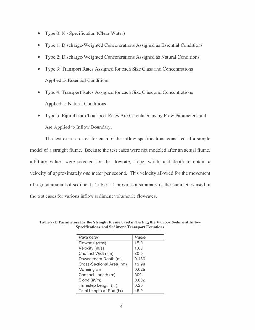
The test cases created for each of the inflow specifications consisted of a simple
model of a straight flume. Because the test cases were not modeled after an actual flume,
arbitrary values were selected for the flowrate, slope, width, and depth to obtain a
velocity of approximately one meter per second. This velocity allowed for the movement
of a good amount of sediment. Table 2-1 provides a summary of the parameters used in
the test cases for various inflow sediment volumetric flowrates.
Table 2-1: Parameters for the Straight Flume Used in Testing the Various Sediment Inflow Specifications and Sediment Transport Equations
Parameter Value Flowrate (cms) 15.0 Velocity (m/s) 1.08 Channel Width (m) 30.0 Downstream Depth (m) 0.466 Cross-Sectional Area (m2) 13.98 Manning’s n 0.025 Channel Length (m) 300 Slope (m/m) 0.002 Timestep Length (hr) 0.25 Total Length of Run (hr) 48.0
15
The test cases for the variation of inflow sediment volumetric flowrate utilized
the Engelund—Hansen transport formula because it applies well to the desired bed
particle size of 0.2 mm—fine sand (Richardson 2001). Test cases for the sediment
inflow concentration assignment (types 1 and 2) consisted of model runs for
concentrations of 0, 10, 100, 1,000, and 10,000 parts per million (ppm). Likewise, the
test cases for sediment inflow transport rates (types 3 and 4) consisted of runs for
transport rates of 0, 1, 5, and 10 cubic meters per second (cms). The clear-water (type 0)
and equilibrium transport rate (type 5) options do not allow for the specification of a
concentration or transport rate. Therefore, a single test case represents each of these two
options. The other parameters required for the model run held the default values
recommended in the User’s Manual for FESMWS FST2DH (Froehlich 2003).
Straight flume test cases with the same dimensions given above provided
appropriate tests for the functionality of the sediment transport capacity equations
available in FST2DH. These equations include the Power formula, the Engelund—
Hansen formula, the Ackers—White formula, the Laursen formula, Yang’s Sand and
Gravel formula, the Meyer-Peter—Mueller formula, the Ackers—White—Day formula,
and the Garbrecht et al. approach, which uses other formulas already mentioned here.
The tests for each of the transport equations included a case for clear-water inflow and a
case for an equilibrium transport rate applied to the inflow boundary. Because most of
the sediment transport equations available in FST2DH apply to the transport of fine
sand, a uniform grain size of 0.20 mm is modeled. The only exception is for the Meyer-
Peter—Mueller formula test case, which modeled a slightly larger grain size of 1.0 mm.
16
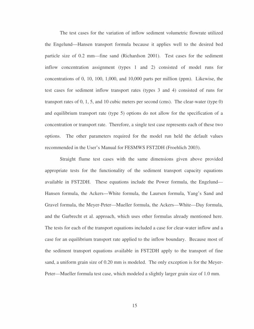
2.2 Straight Flume with Varying Midsection Slopes
Three straight flumes with varying midsection slopes model the affect that various
slopes along a channel have on the FST2DH sediment results. Each flume contains three
segments of varying slope. The length of the flumes was chosen arbitrarily. The selected
velocity of 0.5 m/sec in the upstream and downstream segments allowed for the largest
amount of sediment movement to occur around the steeper, middle section of the flume.
This velocity and arbitrarily-selected values for the width and depth of flow within the
upstream and downstream sections resulted in a calculated flowrate of 12.5 cms. From
this flowrate, the slope was found through Manning’s equation to be 0.00016 m/m for the
upstream and downstream segments. The slope of the middle segment varied from flume
to flume, being very steep in one flume, moderate in the second flume, and quite shallow
in the third. Table 2-2 gives the parameters for the upstream and downstream segments
of all three flumes.
Table 2-2: Parameters for the Upstream and Downstream Segments of the Flumes with Varying Midsection Slopes
Parameter Upstream and Downstream Segments
Flowrate (cms) 12.6 Width (m) 25.0 Downstream Depth (m) 1.0 Cross-Sectional Area (m2) 25.0 Segment Length (m) 100.0 Manning’s n 0.025 Timestep Length (hr) 0.25 Total Length of Run (hr) 48.0

17
Although done somewhat arbitrarily, an attempt was made to select slopes for
each of the middle segments that provided a representation of various water depths and
velocities through the middle of the channel. The results from the test case with the steep
midsection slope given in Table 2-3 suggested that the other two test cases contain a
much shallower midsection slope.
Table 2-3: Slopes for the Middle Segments of the Flumes with Varying Midsection Slopes
Flume Slope (m/m) Steep Midsection 0.0667 Moderate Midsection 0.0067 Shallow Midsection 0.0033
The test cases for the flumes with varying midsection slopes utilize the Engelund-
Hansen transport formula because results from previous tests indicated that it was
functional in FST2DH and because those results appeared reasonable, as will be
described later in this report. The three cases tested both clear-water inflow and
equilibrium transport rate inflow boundary conditions for beds with uniform particle sizes
of 0.08mm, 0.2mm, 2.0mm, and 4.0mm.
Figure 2-1 includes a plot comparing the initial bed elevation profiles for each of
the three flumes.

18
0
2
4
6
8
10
12
0 50 100 150 200 250 300 350
Distance (m)
Ele
vatio
n (m
)
Steep Midsection Moderate Midsection Shallow Midsection
Figure 2-1: Profile of the Three Flumes with Varying Midsection Slope
2.3 Flumes with Contractions
The creation of three simple flumes with contractions allowed for further analysis
of the sediment trends represented by FST2DH when the width of a channel changed in
different ways. All three flumes with contractions had no slope. The first flume
contained a gradual contraction. Its dimensions were chosen arbitrarily. It had a total
length of 350 meters and upstream and downstream widths of 30 meters. The contraction
started 130 meters downstream from the inflow boundary. The narrowest portion
measured 30 meters in length and 10 meters in width, or 40 percent of the original width.
The transitions to and from the contraction to the upstream and downstream widths of the
19
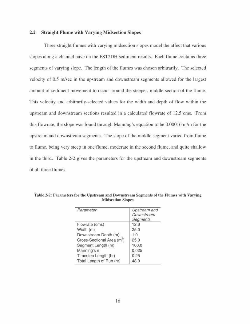
channel each measured 30 meters in length. The tests included cases for both the clear-
water and equilibrium transport rate inflow specifications for each of four different
particle sizes: 0.08 mm, 0.20 mm, 2.0 mm, and 4.0 mm. The parameters for the flume
with a gradual contraction given in Table 2-4 were chosen arbitrarily, with an emphasis
placed on obtaining an upstream velocity of 0.5 meters. This created an increased
velocity through the contraction and provided informative sediment results in that area.
Table 2-4: Parameters for the Flume with a Gradual Contraction
Parameter Upstream and Downstream Segments
Flowrate (cms) 12.5 Velocity (m/s) 0.50 Width (m) 25.0 Downstream Depth (m) 1.0 Cross-Sectional Area (m2) 25.0 Manning’s n 0.025 Slope (m/m) 0.000 Timestep Length (hr) 0.25 Total Length of Run (hr) 48.0
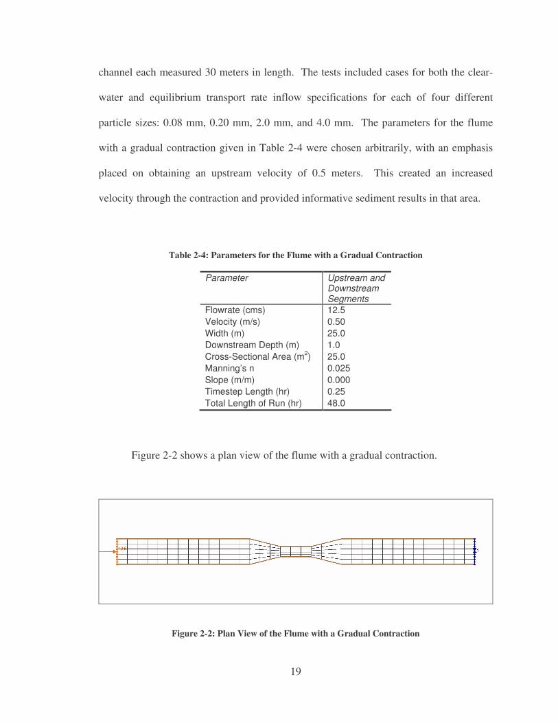
Figure 2-2 shows a plan view of the flume with a gradual contraction.
Figure 2-2: Plan View of the Flume with a Gradual Contraction

20
The second set of test cases for contractions modeled a flume with a long abrupt
contraction. This flume followed the same general description as the one described
above, except that the contraction began and ended abruptly. The parameters given
above in Table 2-4 applied to this set of test cases in addition to those of the flume with a
gradual contraction. Figure 2-3 provides a plan view of the flume with a long abrupt
contraction.
Figure 2-3: Plan View of the Flume with a Long Abrupt Contraction
The final set of test cases for a flume with a contraction modeled a channel that
contained a short abrupt contraction, similar to that often observed at a narrow river
opening under a highway bridge. The test case for the flume with an abrupt contraction
represented a hypothetical channel. The flowrate, depth, widths for the main channel and
the contraction, and other related parameters were again chosen arbitrarily with the intent
of providing a reasonable velocity of 0.5 m/s both upstream and downstream of the
contraction. Table 2-5 lists the main parameters applied to this test case and Figure 2-4
provides a plan view of the flume with a short, abrupt contraction.

21
Table 2-5: Parameters for a Flume with a Short Abrupt Contraction
Parameter Upstream Segment
Contraction Downstream Segment
Flowrate (cms) 12.5 --- 12.5 Velocity (m/s) 0.50 0.50 0.50 Channel Width (m) 25.0 6.5 25.0 Downstream Depth (m) --- --- 0.75 Manning’s n 0.025 0.025 0.025 Segment Length (m) 107.5 10.0 107.5 Slope (m/m) 0.000 0.000 0.000 Timestep Length (hr) 0.25 0.25 0.25 Total Length of Run (hr) 48.0 48.0 48.0
Figure 2-4: Plan View of the Flume with a Short Abrupt Contraction
2.4 SED2D WES Flumes
SED2D WES is the sediment transport program within the TABS-MD Numerical
Modeling System, developed by the U.S. Army Corps of Engineers. It relies on the
hydrodynamic output from a companion program, RMA2 for its sediment calculations,
and therefore only supports the uncoupled option. Thus, if the user desires to obtain a
semi-coupled solution, he or she must manually iterate between the RMA2 hydrodynamic
and SED2D WES sediment models for each timestep to create the final solution.
22
SED2D WES computes the movement of cohesive (clay) or non-cohesive (sand
and gravel) sediment and only supports a single grain size (USACE 2004). The output
from SED2D WES includes one file containing the new bed geometry, a separate file
containing the concentration of sediment and the total change in bed at each node, and a
third file, the bed structure file, that contains information about the consolidation and age
of each of the bed strata for cohesive materials or the thickness of the erodible bed layer
for non-cohesive modeling (USACE 2004).
The research included two different test cases for comparison of results from
FST2DH and SED2D WES. The first case consisted of the flume with a moderate
midsection slope described earlier in this report (section 2.2). Because of the different
input options supported by SED2D WES and FST2DH, the parameters entered for each
of the two sediment simulations differed slightly. However, the input parameters for
SED2D WES were chosen so as to best replicate the same conditions that existed in the
FST2DH test case. Initially, test cases were to be developed for each of the four particle
sizes used in the FST2DH clear water analysis. However, the results from the first test
indicated that doing so would not beneficial, so the first test case only consisted of a
single run in SED2D WES, with a uniform particle size of 0.2 mm. The clear water
condition was applied to the inflow boundary.
The second test case used in the comparison of sediment results from FST2DH
and SED2D consisted of tests for the flume with a gradual contraction. As with the
moderate midsection slope test case, the parameters for the flume with a gradual
contraction were assigned in such a manner that the SED2D WES simulation most
closely matched that described previously for the FST2DH gradual contraction test case.
23
The test cases for SED2D WES contained uniform particle sizes of 0.08 mm, 0.2 mm, 2.0
mm and 4.0 mm. While two of the FST2DH test cases for the gradual flume with clear
water inflow failed to run to completion, the results from SED2D WES could still be
compared with those from the FST2DH equilibrium transport rate cases. The comparison
was appropriate because none of the tests for that flume showed scour or deposition
upstream from the contraction. Therefore, the clear water and equilibrium transport rate
results were identical, as will be explained in more detail in chapter 3. For now, it is
sufficient to note that the comparison between the clear water and equilibrium transport
rate test case results is appropriate for this flume.
While SED2D outputs values at each timestep for the change in bed at each node,
it does not directly provide bed elevations. On the other hand, FST2DH outputs bed
elevations at each node and not the change in bed. Therefore, comparisons of the final
bed elevations for each model were established by creating a new dataset representing the
sum of the initial bed elevation and the final change in bed for the SED2D WES test
cases. Chapter 4 contains the resulting bed elevations from each of the models.
2.5 SAMwin Flumes
The next set of test cases consisted of straight flumes used for comparing
sediment concentrations calculated by FST2DH for equilibrium conditions to those
output by SAMwin. SAMwin applies a variety of sediment transport functions at a
single location in a river to calculate a sediment discharge rating curve based on a
specific hydraulic regime and the gradation of the bed. Output from SAMwin includes
the sediment transport capacity (in tons per day) and sediment concentration (in parts per

24
million) for a river in general equilibrium (Thomas 2002). FST2DH reports
concentrations as the volume of sediment per unit volume of the water-sediment mixture
(Froehlich 2003) and SAMwin reports the concentrations as parts per million (Thomas
2002). Because of this difference, the equilibrium concentrations calculated by FST2DH
were converted to parts per million (ppm) for comparison to SED2D WES output using
standard conversions (Richardson 2001).
The research created simple, straight-flume test cases for comparison between the
concentrations predicted by FST2DH and SAMwin. The parameters arbitrarily selected
for these test cases allowed for the creation of a rectangular flume with a relatively
moderate slope, providing velocities that fell in the desired range of 2.5 fps and 5.5 fps.
Table 2-6 lists the main parameters used in these test cases.
Table 2-6: Parameters for the SAMwin Flume
Parameter Value Upstream Elevation (ft) 1.5 Downstream Elevation (ft) 0.0 Length (ft) 1,000.0 Slope (ft/ft) 0.0015 Width (ft) 70.0 Left Side Slope (Horiz to 1.0) 0.0001 Right Side Slope (Horiz to 1.0) 0.0001 Manning’s n 0.025 Water Temperature (°F) 40.0 Specific Gravity 2.65 Kinematic Viscosity (ft2/sec) 1.662*105
For simplicity, most of the parameters held the default values set by SAMwin.
The same values were assigned to the appropriate parameters during the setup of each
FST2DH simulation. Each test case included a run for a uniform particle size of 0.177
25
mm and one for a uniform size of 1.414 mm. These sizes were chosen because SAMwin
writes out information for these specific size classes and because they fell closest to the
particle sizes used in previous FST2DH test cases.
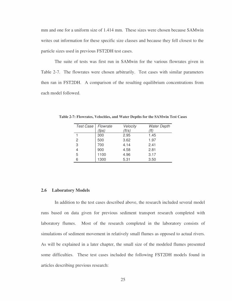
The suite of tests was first run in SAMwin for the various flowrates given in
Table 2-7. The flowrates were chosen arbitrarily. Test cases with similar parameters
then ran in FST2DH. A comparison of the resulting equilibrium concentrations from
each model followed.
Table 2-7: Flowrates, Velocities, and Water Depths for the SAMwin Test Cases
Test Case Flowrate (fps)
Velocity (ft/s)
Water Depth (ft)
1 300 2.95 1.45 2 500 3.62 1.97 3 700 4.14 2.41 4 900 4.58 2.81 5 1100 4.96 3.17 6 1300 5.31 3.50
2.6 Laboratory Models
In addition to the test cases described above, the research included several model
runs based on data given for previous sediment transport research completed with
laboratory flumes. Most of the research completed in the laboratory consists of
simulations of sediment movement in relatively small flumes as opposed to actual rivers.
As will be explained in a later chapter, the small size of the modeled flumes presented
some difficulties. These test cases included the following FST2DH models found in
articles describing previous research:
26
• A flume showing the scour patterns and depths around a pier (Sheppard 2004)
• A flume with varying entrance and exit angles for a long contraction (Dey 2005)
• A basin illustrating the scour from clear water inflow (Duc 2004, Wu 2004)
• A narrow flume demonstrating downstream fining (Seal 1997)
• A wide flume demonstrating downstream fining (Toro-Escobar 2000)
The journal articles listed as references for each bullet in the list above provided
the data for each their respective test cases. The different attempts to simulate the
laboratory models in FST2DH illustrated the effect that the size of the domain had on the
FST2DH simulation results. They also brought to light the need for the various options
that should be functional in FST2DH sediment transport. While research led to many
other laboratory sediment experiments, they required advanced modeling features that are
not currently functional in FST2DH. Detailed information about each of the laboratory
test cases given in this report may be found in their respective papers.
2.7 Deposition in a Reservoir
As part of a journal article, Hotchkiss et al. explained how aggradation occurs due
to backwater when a dam is placed across a river (Hotchkiss 1991). As a river enters a
reservoir, its depth and cross-sectional area increases and the velocity of the water
quickly decreases. The slowing velocity causes some of the sediment within the river to
deposit on the riverbed. Over time, this deposited material forms a delta. The final test
case examined by the FST2DH research modeled this aggradation.
The test case for the flume entering the reservoir contained arbitrary parameters
but still provided insight into how FST2DH models such a situation. The straight flume
27
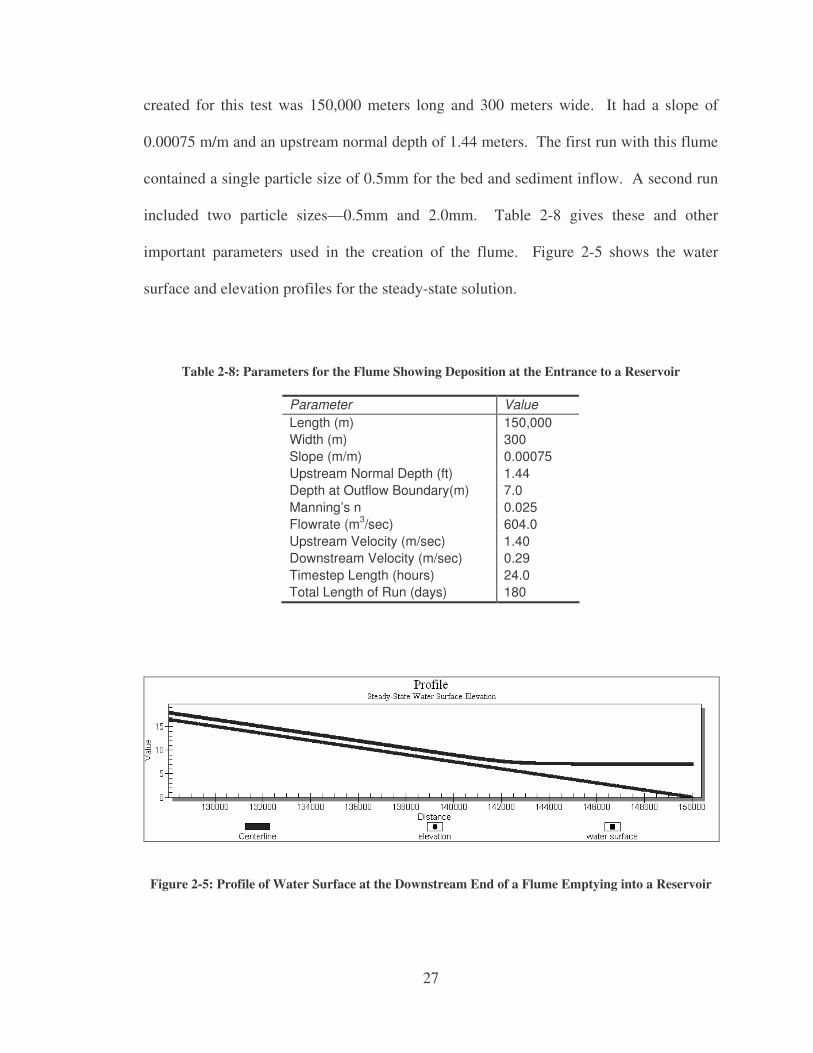
created for this test was 150,000 meters long and 300 meters wide. It had a slope of
0.00075 m/m and an upstream normal depth of 1.44 meters. The first run with this flume
contained a single particle size of 0.5mm for the bed and sediment inflow. A second run
included two particle sizes—0.5mm and 2.0mm. Table 2-8 gives these and other
important parameters used in the creation of the flume. Figure 2-5 shows the water
surface and elevation profiles for the steady-state solution.
Table 2-8: Parameters for the Flume Showing Deposition at the Entrance to a Reservoir
Parameter Value Length (m) 150,000 Width (m) 300 Slope (m/m) 0.00075 Upstream Normal Depth (ft) 1.44 Depth at Outflow Boundary(m) 7.0 Manning’s n 0.025 Flowrate (m3/sec) 604.0 Upstream Velocity (m/sec) 1.40 Downstream Velocity (m/sec) 0.29 Timestep Length (hours) 24.0 Total Length of Run (days) 180
Figure 2-5: Profile of Water Surface at the Downstream End of a Flume Emptying into a Reservoir
28
Research also created a second set of test cases for the flume showing deposition
in a reservoir. The purpose for these test cases was to discover how well FST2DH
handles sediment transport in a long, shallow-sloped river, where a delta forms over a
long period of time. The tests included four different element sizes in an attempt to
create a stable solution over a long model run. The 200,000 meter long, 500 meter wide
flume had a slope of 0.00025, which was about one-third the value of the slope used in
the first reservoir deposition test case. The flume’s upstream velocity was 1.0 m/sec and
the upstream water depth was 2.0 meters. Table 2-9 shows the different element sizes
tested.
Table 2-9: Element Properties for the Test Cases for a Long Flume Emptying into a Reservoir
Test Case Element Length (m)
Element Width (m)
Number of Elements Along Channel Length
A 8,695.7 100 23 B 3,448.3 100 58 C 1,739.1 100 115 D 865.8 100 231

29
3 Presentation of Results: Qualitative Analysis
The purposes of this report include identifying the areas of functionality within
the sediment transport portion of FST2DH and determining the accuracy of the model in
representing the movement of sediment. The research accomplished this in the three
ways described in the previous chapter. This chapter provides and interprets the sediment
results from FST2DH for each of the test cases. The next chapter of this report gives a
comparison of results from FST2DH to those from SAMwin and SED2D WES and also
explains the sediment results from FST2DH models of real laboratory flumes and
compares them to results obtained through previous research.
3.1 Variation of Sediment Inflow and Transport Formulas
The examination of the sediment transport functionality within FST2DH began
with a look at the effects of the variation of the sediment volumetric flow rate that was
specified for the inflow boundary. For these initial runs, the research focused on two
factors which included:
1. Did the model run to completion? If not, when did the failure occur and what
caused it?
2. Does the changing bed elevation for the successful runs seem reasonable and
intuitive?

30
The research moved to a second set of runs that contained variation of the
sediment transport capacity formula applied to the test cases. It was anticipated with
these runs that the bed elevation would not vary from one side of the channel to the other
because the test cases were rectangular flumes of uniform width and constant slope. As
was expected, the variation of bed elevations occurred along the length of the channel for
all test cases given in this section of the report. Figure 3-1 shows an example of the bed
elevation variation along the length of the channel and the lack of variation from one side
of the channel after two days. The time given in the upper left hand corner of this and all
the remaining plan views gives the timestep that the contoured image represents, shown
in days, hours, minutes, and seconds. For these test cases, a longitudinal profile of the
bed elevations presents a clear representation of the simulation. The following sections
present a series of longitudinal profiles for the various test runs.
Figure 3-1: Variation of Bed Elevation along the Length of a Straight Flume
3.1.1 Sediment Volumetric Flow Rate at the Inflow Boundary
As was explained earlier, FST2DH provides the user with six different options for
the specification of a sediment volumetric flow rate at the inflow boundary. All six

31
inflow specifications were tested with the same flume. The test cases with what the
FST2DH documentation refers to as natural conditions both failed within the first hour of
the simulation due to an access violation within the FST2DH program. This included
type 2 (natural sediment concentration) and type 4 (natural transport rate). The test cases
for the remaining sediment flow rate specifications all ran to completion. Their results
follow.
The first profile comes from the test cases with clear water entering the domain
(type 0). The plot (Figure 3-2) includes the initial bed elevation profile along with the
final bed elevation profile after a 48-hour simulation.
Figure 3-2: Initial and Final Bed Elevation Profiles for Clear-Water Inflow
When clear water enters the mesh, the clear-water should quickly pick up
sediment near the inflow boundary, scouring the bed drastically. Further downstream,
once the water is already carrying some sediment, less scour should occur. Figure 3-2
reflects this pattern.
The test cases for the sediment concentration being specified at the inflow
boundary as essential conditions (type 1) all ran to completion. The FST2DH
32
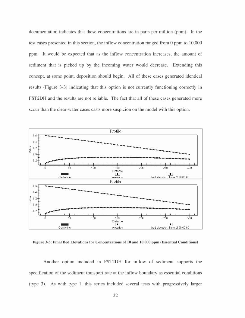
documentation indicates that these concentrations are in parts per million (ppm). In the
test cases presented in this section, the inflow concentration ranged from 0 ppm to 10,000
ppm. It would be expected that as the inflow concentration increases, the amount of
sediment that is picked up by the incoming water would decrease. Extending this
concept, at some point, deposition should begin. All of these cases generated identical
results (Figure 3-3) indicating that this option is not currently functioning correctly in
FST2DH and the results are not reliable. The fact that all of these cases generated more
scour than the clear-water cases casts more suspicion on the model with this option.
Figure 3-3: Final Bed Elevations for Concentrations of 10 and 10,000 ppm (Essential Conditions)
Another option included in FST2DH for inflow of sediment supports the
specification of the sediment transport rate at the inflow boundary as essential conditions
(type 3). As with type 1, this series included several tests with progressively larger

33
transport rates. The resulting bed profiles for each 48-hour simulation were again
identical to each other, regardless of the actual transport rate being specified at the inflow
boundary. This is shown in Figure 3-4. Furthermore, the resulting bed elevation profiles
from these test cases were identical to the profiles shown in Figure 3-3 for the sediment
concentration being specified as essential conditions (type 1). Thus, this research
concluded that FST2DH does not appropriately handle variation in either sediment
concentrations or flow rates assigned to the inflow boundary, and the results obtained
with the use of either option are not reliable.
Figure 3-4: Final Bed Elevations for Sediment Transport Rates of 1 and 10 cms (Essential Conditions)
The final option included in FST2DH for inflow of sediment applies an
equilibrium sediment transport rate to the inflow boundary (type 5). In this case,
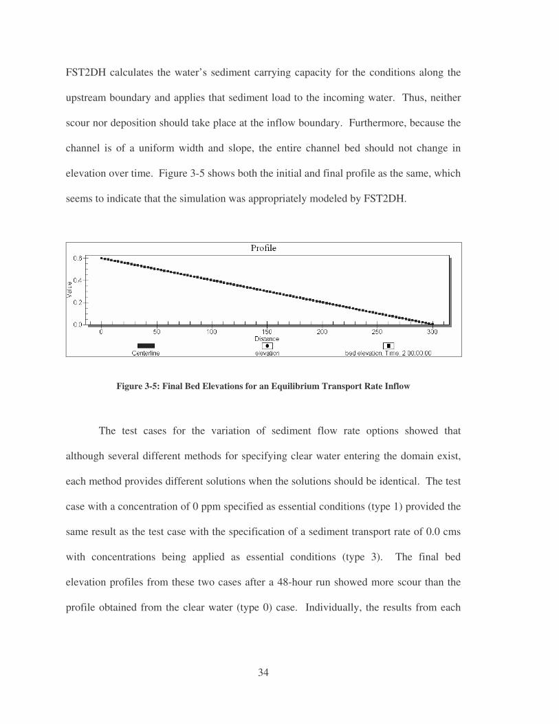
34
FST2DH calculates the water’s sediment carrying capacity for the conditions along the
upstream boundary and applies that sediment load to the incoming water. Thus, neither
scour nor deposition should take place at the inflow boundary. Furthermore, because the
channel is of a uniform width and slope, the entire channel bed should not change in
elevation over time. Figure 3-5 shows both the initial and final profile as the same, which
seems to indicate that the simulation was appropriately modeled by FST2DH.
Figure 3-5: Final Bed Elevations for an Equilibrium Transport Rate Inflow
The test cases for the variation of sediment flow rate options showed that
although several different methods for specifying clear water entering the domain exist,
each method provides different solutions when the solutions should be identical. The test
case with a concentration of 0 ppm specified as essential conditions (type 1) provided the
same result as the test case with the specification of a sediment transport rate of 0.0 cms
with concentrations being applied as essential conditions (type 3). The final bed
elevation profiles from these two cases after a 48-hour run showed more scour than the
profile obtained from the clear water (type 0) case. Individually, the results from each
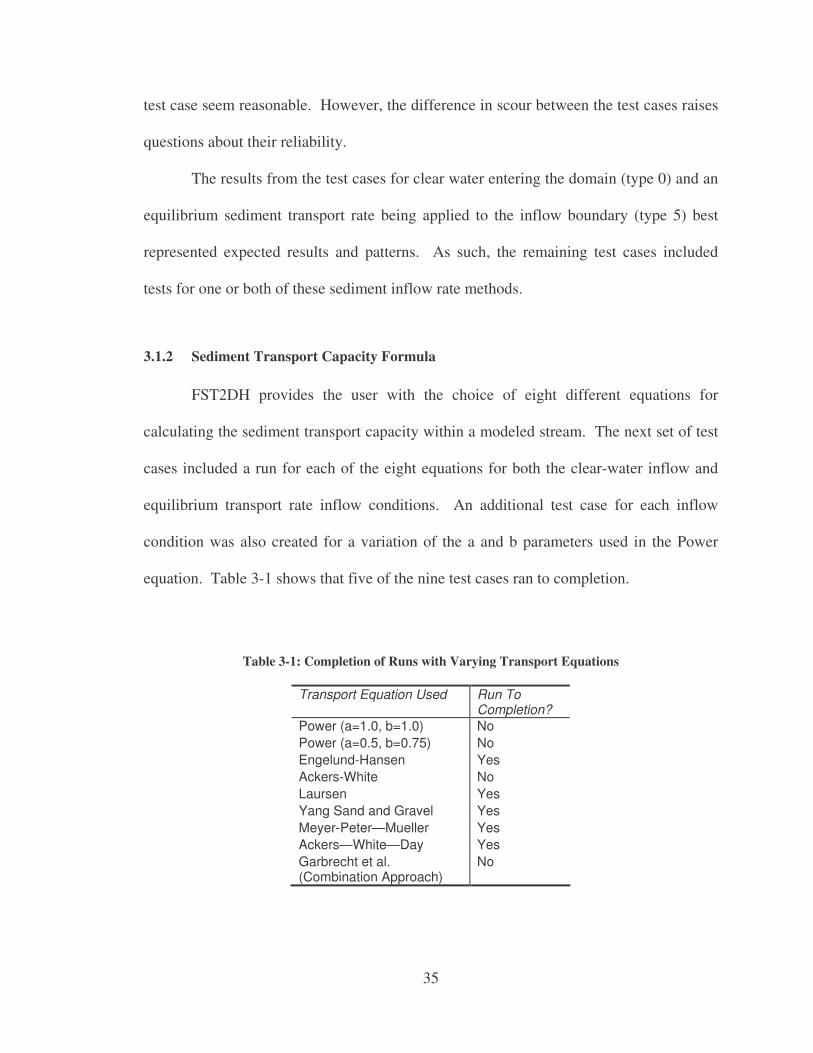
35
test case seem reasonable. However, the difference in scour between the test cases raises
questions about their reliability.
The results from the test cases for clear water entering the domain (type 0) and an
equilibrium sediment transport rate being applied to the inflow boundary (type 5) best
represented expected results and patterns. As such, the remaining test cases included
tests for one or both of these sediment inflow rate methods.
3.1.2 Sediment Transport Capacity Formula
FST2DH provides the user with the choice of eight different equations for
calculating the sediment transport capacity within a modeled stream. The next set of test
cases included a run for each of the eight equations for both the clear-water inflow and
equilibrium transport rate inflow conditions. An additional test case for each inflow
condition was also created for a variation of the a and b parameters used in the Power
equation. Table 3-1 shows that five of the nine test cases ran to completion.
Table 3-1: Completion of Runs with Varying Transport Equations
Transport Equation Used Run To Completion?
Power (a=1.0, b=1.0) No Power (a=0.5, b=0.75) No Engelund-Hansen Yes Ackers-White No Laursen Yes Yang Sand and Gravel Yes Meyer-Peter—Mueller Yes Ackers—White—Day Yes Garbrecht et al. (Combination Approach)
No

36
The runs that failed most commonly provided the error message, “!ERROR -
RowCount > MaxFrontWidth in xAssemble. Stopping…” The test cases that ran to
completion all did so for both the clear-water and equilibrium transport rate inflow
conditions. Furthermore, all the ones that failed did so for both inflow conditions. The
successful models that were assigned an equilibrium transport rate inflow condition all
maintained the same bed profile as that of the initial bed throughout the entire 48-hour
simulation, regardless of sediment transport equation used. This provides evidence that
the equilibrium inflow specification works appropriately with the currently-functional
transport equations in that FST2DH is calculating the correct transport rate so as to keep
scour and deposition from occurring.
The test cases with clear water entering the mesh all resulted in scouring of the
bed. The amount of erosion varied with the transport equation being used. This makes
sense, as the different equations each use different methods to calculate the transport
capacity of the channel, which results in a different amount of sediment being carried
away in each case. None of the test case results suggested that deposition had occurred.
However, this is not surprising since the slope and cross section remain constant and
clean, sediment-hungry water is entering the domain.
Figure 3-6 provides a comparison of the initial bed profile and final bed profiles
after a 48-hour simulation using the Engelund—Hansen formula, the Laursen formula,
the Yang Sand and Gravel formula, the Meyer-Peter—Mueller formula, and the
Ackers—White—Day formula.
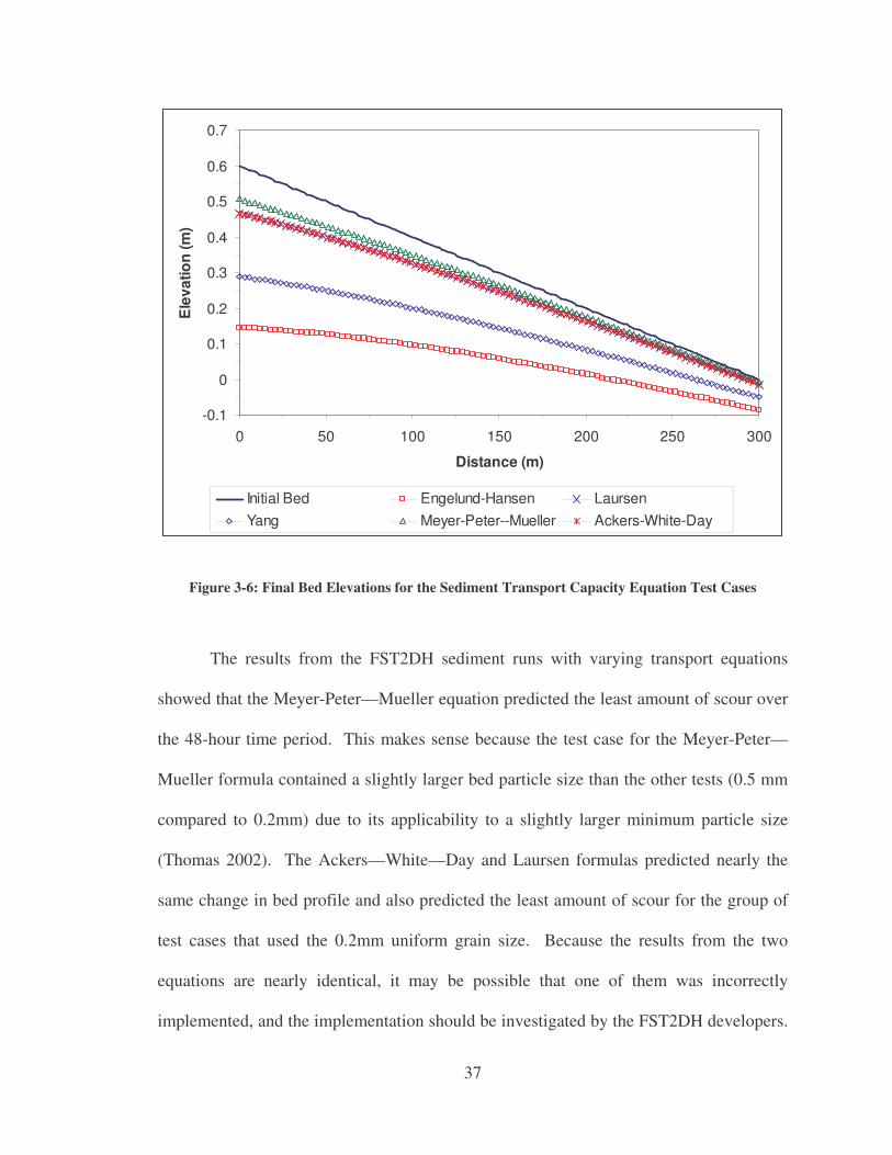
37
-0.1
0
0.1
0.2
0.3
0.4
0.5
0.6
0.7
0 50 100 150 200 250 300
Distance (m)
Ele
vatio
n (m
)
Initial Bed Engelund-Hansen LaursenYang Meyer-Peter--Mueller Ackers-White-Day
Figure 3-6: Final Bed Elevations for the Sediment Transport Capacity Equation Test Cases
The results from the FST2DH sediment runs with varying transport equations
showed that the Meyer-Peter—Mueller equation predicted the least amount of scour over
the 48-hour time period. This makes sense because the test case for the Meyer-Peter—
Mueller formula contained a slightly larger bed particle size than the other tests (0.5 mm
compared to 0.2mm) due to its applicability to a slightly larger minimum particle size
(Thomas 2002). The Ackers—White—Day and Laursen formulas predicted nearly the
same change in bed profile and also predicted the least amount of scour for the group of
test cases that used the 0.2mm uniform grain size. Because the results from the two
equations are nearly identical, it may be possible that one of them was incorrectly
implemented, and the implementation should be investigated by the FST2DH developers.
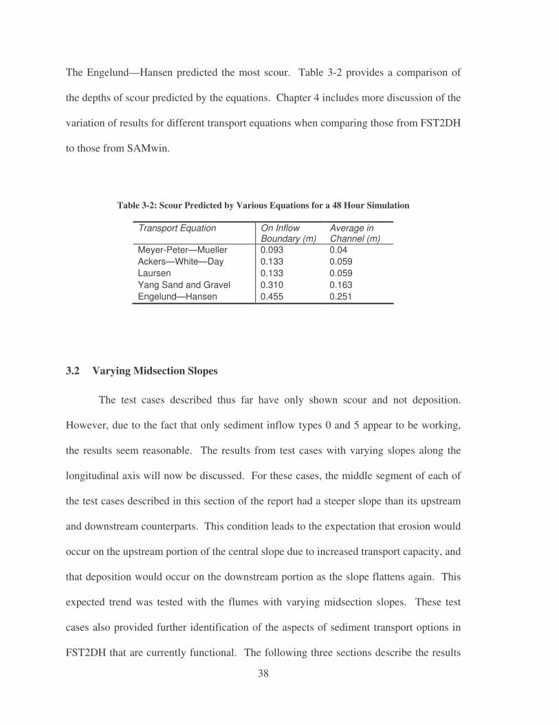
38
The Engelund—Hansen predicted the most scour. Table 3-2 provides a comparison of
the depths of scour predicted by the equations. Chapter 4 includes more discussion of the
variation of results for different transport equations when comparing those from FST2DH
to those from SAMwin.
Table 3-2: Scour Predicted by Various Equations for a 48 Hour Simulation
Transport Equation On Inflow Boundary (m)
Average in Channel (m)
Meyer-Peter—Mueller 0.093 0.04 Ackers—White—Day 0.133 0.059 Laursen 0.133 0.059 Yang Sand and Gravel 0.310 0.163 Engelund—Hansen 0.455 0.251
3.2 Varying Midsection Slopes
The test cases described thus far have only shown scour and not deposition.
However, due to the fact that only sediment inflow types 0 and 5 appear to be working,
the results seem reasonable. The results from test cases with varying slopes along the
longitudinal axis will now be discussed. For these cases, the middle segment of each of
the test cases described in this section of the report had a steeper slope than its upstream
and downstream counterparts. This condition leads to the expectation that erosion would
occur on the upstream portion of the central slope due to increased transport capacity, and
that deposition would occur on the downstream portion as the slope flattens again. This
expected trend was tested with the flumes with varying midsection slopes. These test
cases also provided further identification of the aspects of sediment transport options in
FST2DH that are currently functional. The following three sections describe the results

39
from the three test cases with varying midsection slopes. The tests included three central
slopes: 0.0667 m/m, 0.0067 m/m, and 0.0033 m/m. The results from the test case with
the steepest slope will be given first, followed by those from the moderate slope test case,
and then those from the case with the shallowest slope will be provided.
3.2.1 Steep Midsection Slope
The steady state hydrodynamic solution showed that the slope of the channel’s
middle segment was steep enough to create supercritical flow through that section,
resulting in a hydraulic jump near the break in slope at the downstream end of the steeper
section, as the water jumped back to subcritical flow downstream. This is illustrated in
the profiles of the initial bed elevation and the water surface calculated by a steady-state
hydrodynamic run of FST2DH and shown in Figure 3-7. All of the test cases for the
steep midsection slope failed to run to completion once the sediment calculations were
added. Thus, neither the variation of the type of sediment inflow specification (clear-
water or equilibrium transport rate), nor the variation of sediment particle size seemed to
Figure 3-7: Steady-State Bed and Water Depth Profiles for a Flume with a Steep Midsection Slope

40
affect the outcome. The instability within the sediment model run may have been caused
by the presence of the hydraulic jump and/or the shallow water depth (0.13 meters) just
upstream of the jump.
3.2.2 Moderate Midsection Slope
The steady-state hydrodynamic solution for the test cases with a moderate
midsection slope (0.0067 m/m) shows that the flow throughout the entire channel
remained subcritical. Furthermore, the solution, shown in Figure 3-8, suggests that the
backwater curve from the change in the bed extends upstream beyond the inflow
boundary.
Figure 3-8: Initial Bed Elevation and Water Surface for a Flume with a Moderate Midsection Slope
The test cases for a moderate midsection slope showed that the simulation of
sediment transport in FST2DH was much more stable for the equilibrium transport rate
option for the inflow boundary than it was for the clear-water inflow case. While only
one of the four test cases with clear water entering the mesh ran to completion (the case

41
for 0.2mm), all four of the test cases with the equilibrium transport rate option ran to
completion.
The next two figures (Figure 3-9 and Figure 3-10) show the progression of the
change in the bed profile throughout the 48-hour simulation for the test case with clear
water and a uniform grain size of 0.2mm. Each plot includes the initial bed elevations for
comparison.
Figure 3-9: Bed Elevations for the Clear-Water Moderate Midsection Slope Flume with a Uniform Particle Size of 0.2mm at 15 Minutes, 1 Hour, and 4 Hours

42
Figure 3-10: Bed Elevations for the Clear-Water Moderate Midsection Slope Flume with a Uniform Particle Size of 0.2mm at 6 Hours, 12 Hours, 24 Hours, and 48 Hours
The profiles in the figures show that, as would be expected, scouring began right
at the upstream boundary, with the clear water picking up whatever sediment it can. The
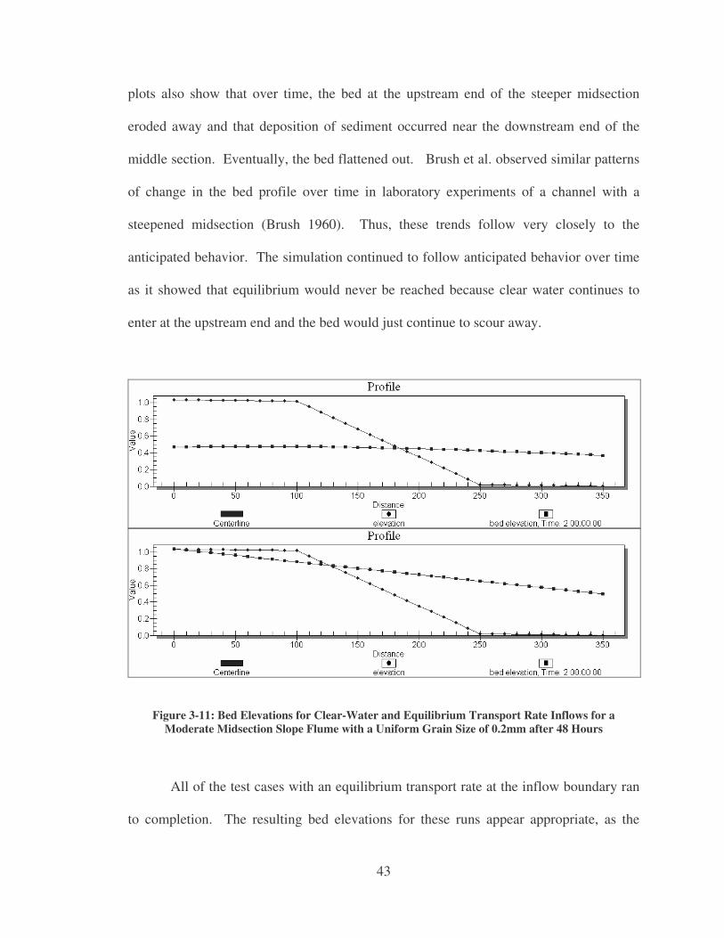
43
plots also show that over time, the bed at the upstream end of the steeper midsection
eroded away and that deposition of sediment occurred near the downstream end of the
middle section. Eventually, the bed flattened out. Brush et al. observed similar patterns
of change in the bed profile over time in laboratory experiments of a channel with a
steepened midsection (Brush 1960). Thus, these trends follow very closely to the
anticipated behavior. The simulation continued to follow anticipated behavior over time
as it showed that equilibrium would never be reached because clear water continues to
enter at the upstream end and the bed would just continue to scour away.
Figure 3-11: Bed Elevations for Clear-Water and Equilibrium Transport Rate Inflows for a Moderate Midsection Slope Flume with a Uniform Grain Size of 0.2mm after 48 Hours
All of the test cases with an equilibrium transport rate at the inflow boundary ran
to completion. The resulting bed elevations for these runs appear appropriate, as the
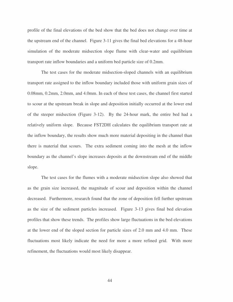
44
profile of the final elevations of the bed show that the bed does not change over time at
the upstream end of the channel. Figure 3-11 gives the final bed elevations for a 48-hour
simulation of the moderate midsection slope flume with clear-water and equilibrium
transport rate inflow boundaries and a uniform bed particle size of 0.2mm.
The test cases for the moderate midsection-sloped channels with an equilibrium
transport rate assigned to the inflow boundary included those with uniform grain sizes of
0.08mm, 0.2mm, 2.0mm, and 4.0mm. In each of these test cases, the channel first started
to scour at the upstream break in slope and deposition initially occurred at the lower end
of the steeper midsection (Figure 3-12). By the 24-hour mark, the entire bed had a
relatively uniform slope. Because FST2DH calculates the equilibrium transport rate at
the inflow boundary, the results show much more material depositing in the channel than
there is material that scours. The extra sediment coming into the mesh at the inflow
boundary as the channel’s slope increases deposits at the downstream end of the middle
slope.
The test cases for the flumes with a moderate midsection slope also showed that
as the grain size increased, the magnitude of scour and deposition within the channel
decreased. Furthermore, research found that the zone of deposition fell further upstream
as the size of the sediment particles increased. Figure 3-13 gives final bed elevation
profiles that show these trends. The profiles show large fluctuations in the bed elevations
at the lower end of the sloped section for particle sizes of 2.0 mm and 4.0 mm. These
fluctuations most likely indicate the need for more a more refined grid. With more
refinement, the fluctuations would most likely disappear.
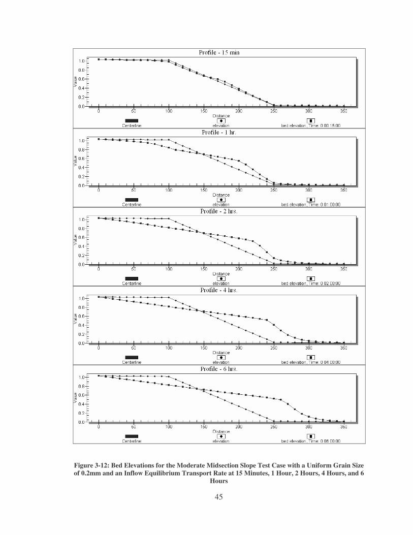
45
Figure 3-12: Bed Elevations for the Moderate Midsection Slope Test Case with a Uniform Grain Size of 0.2mm and an Inflow Equilibrium Transport Rate at 15 Minutes, 1 Hour, 2 Hours, 4 Hours, and 6
Hours

46
Figure 3-13: Bed Elevations after 48 Hours for a Moderate Midsection Slope Flume with an Inflow Equilibrium Transport Rate and Particle Sizes of 0.08mm, 0.2mm, 2.0mm, and 4.0mm
3.2.3 Shallow Midsection Slope
All but one of the test cases for the shallow midsection slope (0.0033 m/m) ran to
completion. The clear-water, 0.08mm test case failed, giving the error, “!ERROR -

47
RowCount > MaxFrontWidth in xAssemble. Stopping…” during calculations for the first
timestep. The remaining test cases that were successful provide seemingly reasonable
results.
The steady-state solution for the flume with a shallow midsection slope showed
that the change in slope had an effect on the water surface elevation along the
longitudinal axis. The solution further suggested that a backwater curve extends
upstream of the inflow boundary (Figure 3-14) and that if the quantity of scour at the
inflow boundary of a model of a real flume needed to be identified, the inflow boundary
should be pulled further upstream.
Figure 3-14: Initial Bed Elevation and Water Surface for the Flume with a Shallow Midsection Slope
The results from the shallow midsection slope test cases provided a pattern similar
to that observed in the results from the moderate midsection slope test cases—that of the
gradual flattening out of the bed over time. Similarly, the erosion in the shallow
midsection test cases first occurred along the upstream segment of the channel and
deposition first occurred almost immediately downstream. This result was expected
because the maximum velocity occurred near the first break in slope and then the velocity
quickly slowed down soon thereafter, allowing the sediment to be picked up by the water

48
briefly and then quickly deposited again. As was also seen with the moderate midsection
test cases, the entire bed of the shallow midsection cases flattened out over the two-day
simulation. Again, this same pattern was observed in laboratory experiments by Brush et
al. (Brush 1960). The next two figures (Figure 3-15 and Figure 3-16) illustrate this
change in bed for the clear-water, 0.2mm uniform grain size test case. Additional
simulation time would show that the bed does eventually flatten out at the downstream
end of the channel.
Figure 3-15: Beginning Stages of the Bed Flattening over Time for the Clear-Water, Shallow Midsection Test Case with a Uniform Grain Size of 0.2mm
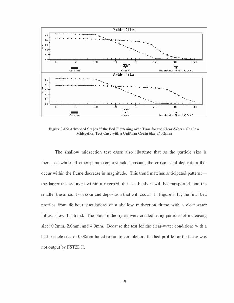
49
Figure 3-16: Advanced Stages of the Bed Flattening over Time for the Clear-Water, Shallow Midsection Test Case with a Uniform Grain Size of 0.2mm
The shallow midsection test cases also illustrate that as the particle size is
increased while all other parameters are held constant, the erosion and deposition that
occur within the flume decrease in magnitude. This trend matches anticipated patterns—
the larger the sediment within a riverbed, the less likely it will be transported, and the
smaller the amount of scour and deposition that will occur. In Figure 3-17, the final bed
profiles from 48-hour simulations of a shallow midsection flume with a clear-water
inflow show this trend. The plots in the figure were created using particles of increasing
size: 0.2mm, 2.0mm, and 4.0mm. Because the test for the clear-water conditions with a
bed particle size of 0.08mm failed to run to completion, the bed profile for that case was
not output by FST2DH.
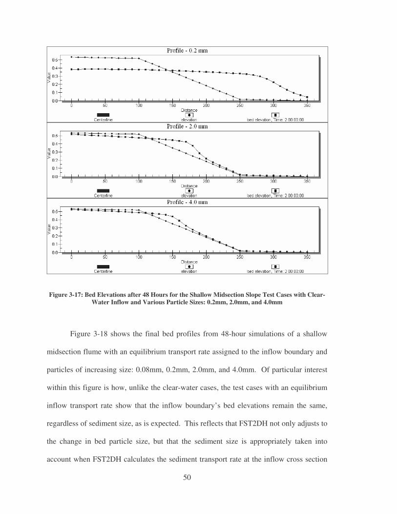
50
Figure 3-17: Bed Elevations after 48 Hours for the Shallow Midsection Slope Test Cases with Clear-Water Inflow and Various Particle Sizes: 0.2mm, 2.0mm, and 4.0mm
Figure 3-18 shows the final bed profiles from 48-hour simulations of a shallow
midsection flume with an equilibrium transport rate assigned to the inflow boundary and
particles of increasing size: 0.08mm, 0.2mm, 2.0mm, and 4.0mm. Of particular interest
within this figure is how, unlike the clear-water cases, the test cases with an equilibrium
inflow transport rate show that the inflow boundary’s bed elevations remain the same,
regardless of sediment size, as is expected. This reflects that FST2DH not only adjusts to
the change in bed particle size, but that the sediment size is appropriately taken into
account when FST2DH calculates the sediment transport rate at the inflow cross section
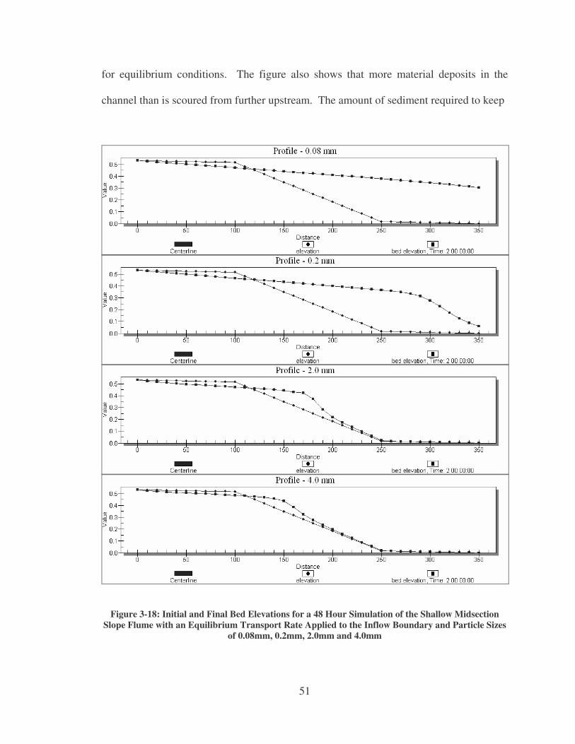
51
for equilibrium conditions. The figure also shows that more material deposits in the
channel than is scoured from further upstream. The amount of sediment required to keep
Figure 3-18: Initial and Final Bed Elevations for a 48 Hour Simulation of the Shallow Midsection Slope Flume with an Equilibrium Transport Rate Applied to the Inflow Boundary and Particle Sizes
of 0.08mm, 0.2mm, 2.0mm and 4.0mm
52
equilibrium conditions at the upstream end of the channel increases as the slope in that
region becomes steeper over time. Thus, FST2DH gradually increases the transport rate
of sediment entering the mesh over the course of the simulation. Upon entering the
mesh, the water holds a lot of sediment. When the sediment-laden water slows down in
the downstream portion of the mesh, much of the sediment it was carrying deposits. This
increases the downstream bed elevations very quickly over time, but does not provide for
much scouring upstream.
Another observation made in the evaluation of the results from the shallow
midsection slope test cases is that the change in the geometry with the movement of the
bed has a great effect on the channel’s hydrodynamic parameters over time. As the bed
continues to flatten out with each new timestep, the range of velocities for each new
timestep decreases. This result follows anticipated patterns, as flatter channels tend to
result in a more even velocity distribution throughout the domain than do channels with
varying slopes. Figure 3-19 shows the shift in the location of the maximum velocity. It
also shows that the range of velocities observed for a given timestep slowly decreases
through time. The profiles given in the figure are for the clear-water 0.2mm uniform bed
grain size test case. At the beginning of the model run, the velocity profile showed
somewhat of a sharp peak where the bed’s slope increased dramatically. After the six-
hour mark, the general shape of the profile remained the same but the magnitude and
location of the peak velocity changed. Furthermore, the decrease of velocity that
occurred in the downstream portion of the channel became more abrupt over time.

53
Figure 3-19: Change in Velocity Magnitude over 48 Hours for the Shallow Midsection Slope Flume with Clear-Water Inflow and a Particle Size of 0.2mm
54
3.3 Flumes with Contractions
This section contains the sediment results from the test cases for the three flumes
with different midsection contractions. It provides and briefly explains the patterns
observed in the final bed elevations for model runs of various types of contractions,
inflow sediment specifications, and sediment particle sizes. The change in channel width
through the contraction forces an uneven distribution of scour and deposition across a
given cross-section. Because of this, the patterns of scour and deposition are best seen in
plan view. The results provided in this section will thus show contoured bed elevations
as well as centerline profiles of the bed elevations.
3.3.1 Gradual Contraction
The test cases for a flume with a gradual contraction show a changing location
and magnitude of scour through the narrowest portion of the contraction. They also show
how the scour and deposition are distributed within the channel as it begins to widen at
the end of the contraction. The steady state hydrodynamic solution for the gradual
contraction flume (Figure 3-20) shows the backing up of water upstream from the
contraction with a centerline profile and spatial distribution of water depth.
The velocity dramatically increases through the contraction and then drops again
to nearly the same magnitude as upstream of the contraction. Figure 3-21 shows the
profile and spatial distribution of the initial velocity magnitude.

55
Figure 3-20: Steady-State Solution for Water Depth in the Flume with a Gradual Contraction
Figure 3-21: Steady-State Solution for Velocity Magnitude for the Flume with a Gradual Contraction
The research included gradual contraction test cases for both the clear-water and
equilibrium sediment transport rate conditions with uniform particle sizes of 0.08, 0.2,
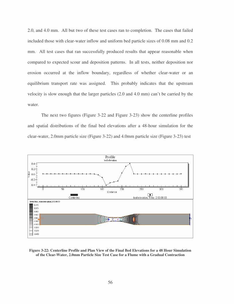
56
2.0, and 4.0 mm. All but two of these test cases ran to completion. The cases that failed
included those with clear-water inflow and uniform bed particle sizes of 0.08 mm and 0.2
mm. All test cases that ran successfully produced results that appear reasonable when
compared to expected scour and deposition patterns. In all tests, neither deposition nor
erosion occurred at the inflow boundary, regardless of whether clear-water or an
equilibrium transport rate was assigned. This probably indicates that the upstream
velocity is slow enough that the larger particles (2.0 and 4.0 mm) can’t be carried by the
water.
The next two figures (Figure 3-22 and Figure 3-23) show the centerline profiles
and spatial distributions of the final bed elevations after a 48-hour simulation for the
clear-water, 2.0mm particle size (Figure 3-22) and 4.0mm particle size (Figure 3-23) test
Figure 3-22: Centerline Profile and Plan View of the Final Bed Elevations for a 48 Hour Simulation of the Clear-Water, 2.0mm Particle Size Test Case for a Flume with a Gradual Contraction
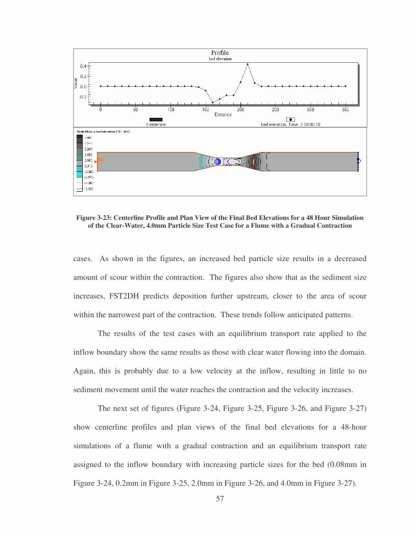
57
Figure 3-23: Centerline Profile and Plan View of the Final Bed Elevations for a 48 Hour Simulation of the Clear-Water, 4.0mm Particle Size Test Case for a Flume with a Gradual Contraction
cases. As shown in the figures, an increased bed particle size results in a decreased
amount of scour within the contraction. The figures also show that as the sediment size
increases, FST2DH predicts deposition further upstream, closer to the area of scour
within the narrowest part of the contraction. These trends follow anticipated patterns.
The results of the test cases with an equilibrium transport rate applied to the
inflow boundary show the same results as those with clear water flowing into the domain.
Again, this is probably due to a low velocity at the inflow, resulting in little to no
sediment movement until the water reaches the contraction and the velocity increases.
The next set of figures (Figure 3-24, Figure 3-25, Figure 3-26, and Figure 3-27)
show centerline profiles and plan views of the final bed elevations for a 48-hour
simulations of a flume with a gradual contraction and an equilibrium transport rate
assigned to the inflow boundary with increasing particle sizes for the bed (0.08mm in
Figure 3-24, 0.2mm in Figure 3-25, 2.0mm in Figure 3-26, and 4.0mm in Figure 3-27).
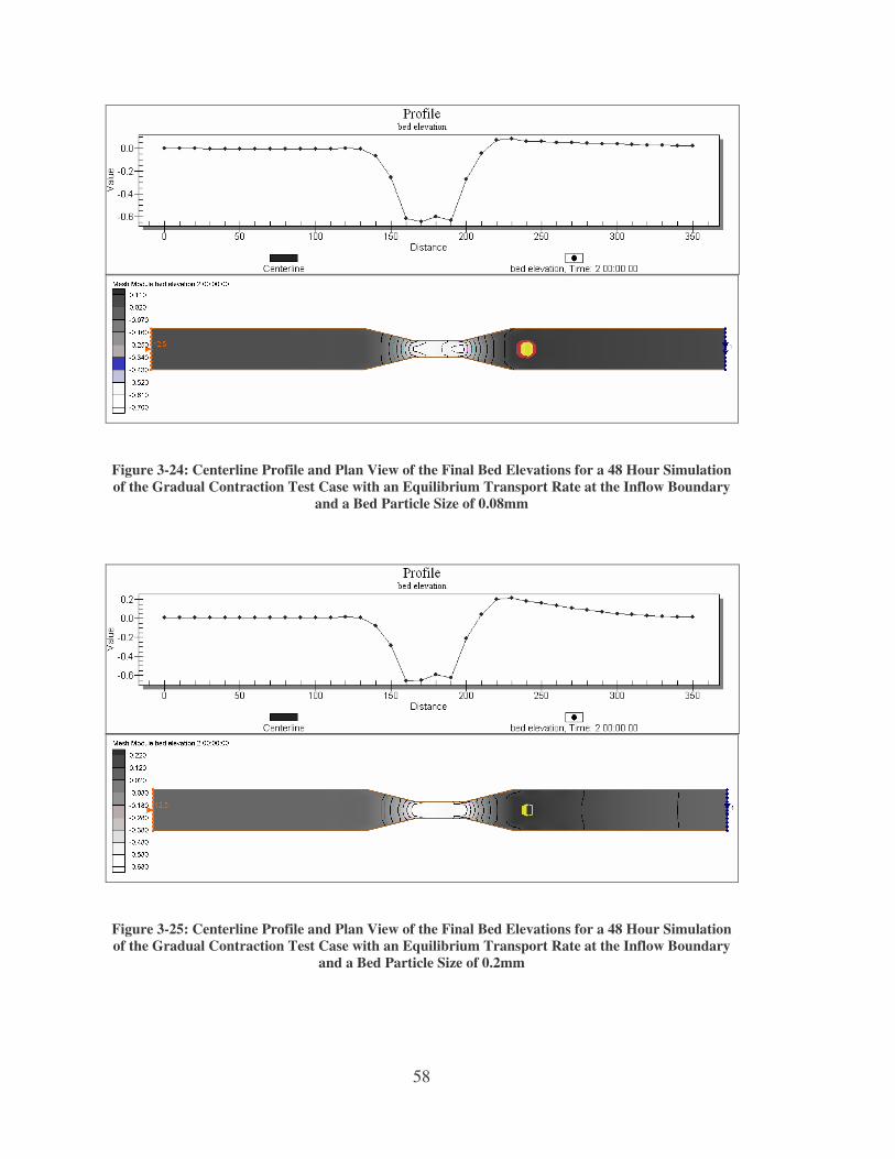
58
Figure 3-24: Centerline Profile and Plan View of the Final Bed Elevations for a 48 Hour Simulation of the Gradual Contraction Test Case with an Equilibrium Transport Rate at the Inflow Boundary
and a Bed Particle Size of 0.08mm
Figure 3-25: Centerline Profile and Plan View of the Final Bed Elevations for a 48 Hour Simulation of the Gradual Contraction Test Case with an Equilibrium Transport Rate at the Inflow Boundary
and a Bed Particle Size of 0.2mm

59
Figure 3-26: Centerline Profile and Plan View of the Final Bed Elevations for a 48 Hour Simulation of the Gradual Contraction Test Case with an Equilibrium Transport Rate at the Inflow Boundary
and a Bed Particle Size of 2.0mm
Figure 3-27: Centerline Profile and Plan View of the Final Bed Elevations for a 48-hour Simulation of the Gradual Contraction Test Case with an Equilibrium Transport Rate at the Inflow Boundary
and a Bed Particle Size of 4.0mm
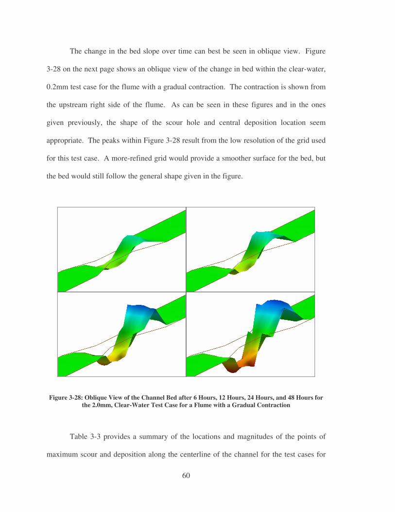
60
The change in the bed slope over time can best be seen in oblique view. Figure
3-28 on the next page shows an oblique view of the change in bed within the clear-water,
0.2mm test case for the flume with a gradual contraction. The contraction is shown from
the upstream right side of the flume. As can be seen in these figures and in the ones
given previously, the shape of the scour hole and central deposition location seem
appropriate. The peaks within Figure 3-28 result from the low resolution of the grid used
for this test case. A more-refined grid would provide a smoother surface for the bed, but
the bed would still follow the general shape given in the figure.
Figure 3-28: Oblique View of the Channel Bed after 6 Hours, 12 Hours, 24 Hours, and 48 Hours for the 2.0mm, Clear-Water Test Case for a Flume with a Gradual Contraction
Table 3-3 provides a summary of the locations and magnitudes of the points of
maximum scour and deposition along the centerline of the channel for the test cases for
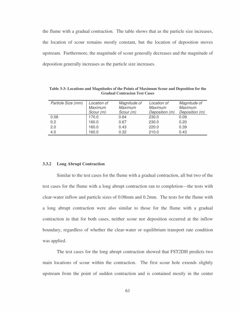
61
the flume with a gradual contraction. The table shows that as the particle size increases,
the location of scour remains mostly constant, but the location of deposition moves
upstream. Furthermore, the magnitude of scour generally decreases and the magnitude of
deposition generally increases as the particle size increases.
Table 3-3: Locations and Magnitudes of the Points of Maximum Scour and Deposition for the Gradual Contracion Test Cases
Particle Size (mm) Location of Maximum Scour (m)
Magnitude of Maximum Scour (m)
Location of Maximum Deposition (m)
Magnitude of Maximum Deposition (m)
0.08 170.0 0.64 230.0 0.09 0.2 160.0 0.67 230.0 0.20 2.0 160.0 0.43 220.0 0.39 4.0 160.0 0.32 210.0 0.43
3.3.2 Long Abrupt Contraction
Similar to the test cases for the flume with a gradual contraction, all but two of the
test cases for the flume with a long abrupt contraction ran to completion—the tests with
clear-water inflow and particle sizes of 0.08mm and 0.2mm. The tests for the flume with
a long abrupt contraction were also similar to those for the flume with a gradual
contraction in that for both cases, neither scour nor deposition occurred at the inflow
boundary, regardless of whether the clear-water or equilibrium transport rate condition
was applied.
The test cases for the long abrupt contraction showed that FST2DH predicts two
main locations of scour within the contraction. The first scour hole extends slightly
upstream from the point of sudden contraction and is contained mostly in the center

62
portion of the channel, and not along the banks. The second location of deepest scour
occurs at the end of the contraction and the area of deposition is distributed around the
downstream end of the scour hole and lies in the wider portion of the channel. The
deposition is observed close to the contraction along the sides of the channel and further
from it in the center of the channel. This pattern matches expectations, as the highest
velocities caused by the contraction will lie in the center of the channel, which means that
sediment will be carried further within the center of the channel. As the velocity slows
down upon exiting the contraction, the highest velocity will remain in the center of the
channel until the velocity across the channel becomes fairly uniform. These results are
shown in Figure 3-29 for the equilibrium transport rate test case for a bed particle size of
0.2 mm.
Figure 3-29: Plan View of the Bed Elevations after 48 Hours for the Equilibrium Transport Rate, 0.2mm Grain Size Test Case for a Flume with a Long Abrupt Contraction
The test cases for the long abrupt contraction show that as the bed particle size
increases, the depth of the scour hole generally decreases. Also, as the particle size
increases, the zone of deposition along the centerline of the channel decreases in length
and increases in depth. The bed profiles for various particle sizes given in Figure 3-30
and Figure 3-31 illustrate these findings.
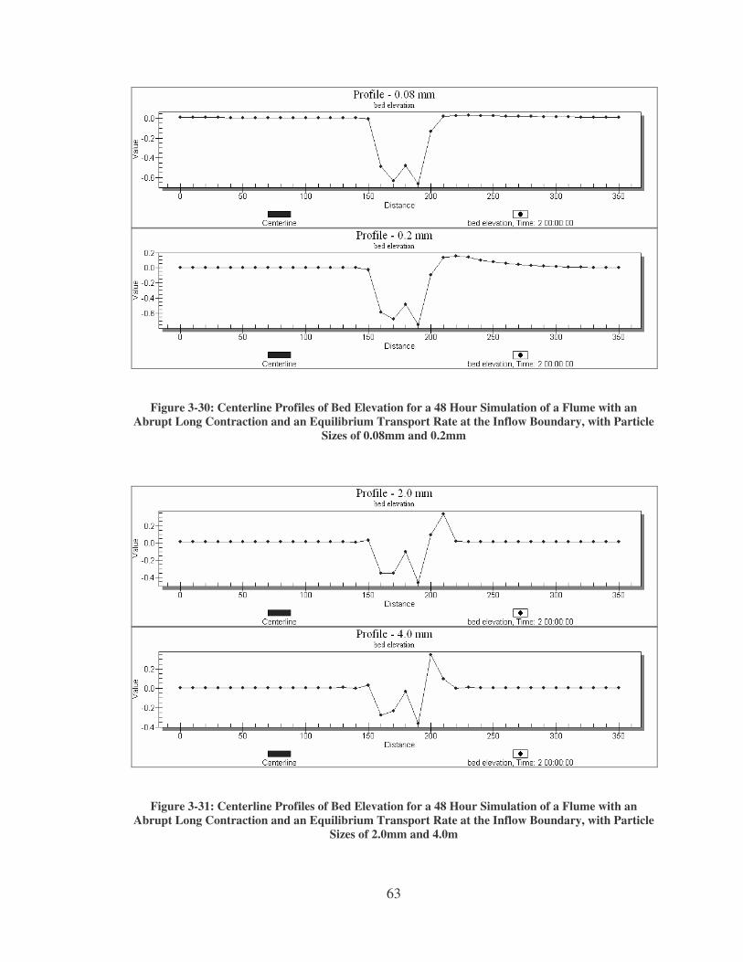
63
Figure 3-30: Centerline Profiles of Bed Elevation for a 48 Hour Simulation of a Flume with an Abrupt Long Contraction and an Equilibrium Transport Rate at the Inflow Boundary, with Particle
Sizes of 0.08mm and 0.2mm
Figure 3-31: Centerline Profiles of Bed Elevation for a 48 Hour Simulation of a Flume with an Abrupt Long Contraction and an Equilibrium Transport Rate at the Inflow Boundary, with Particle
Sizes of 2.0mm and 4.0m
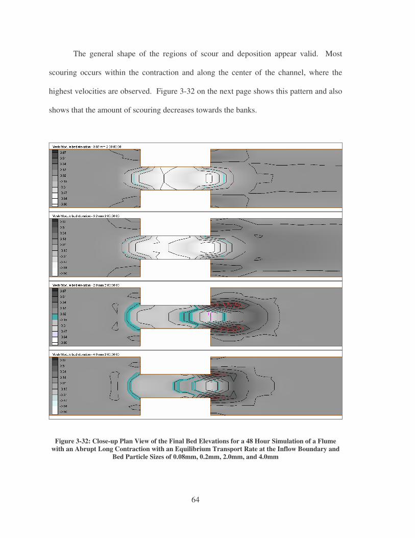
64
The general shape of the regions of scour and deposition appear valid. Most
scouring occurs within the contraction and along the center of the channel, where the
highest velocities are observed. Figure 3-32 on the next page shows this pattern and also
shows that the amount of scouring decreases towards the banks.
Figure 3-32: Close-up Plan View of the Final Bed Elevations for a 48 Hour Simulation of a Flume with an Abrupt Long Contraction with an Equilibrium Transport Rate at the Inflow Boundary and
Bed Particle Sizes of 0.08mm, 0.2mm, 2.0mm, and 4.0mm
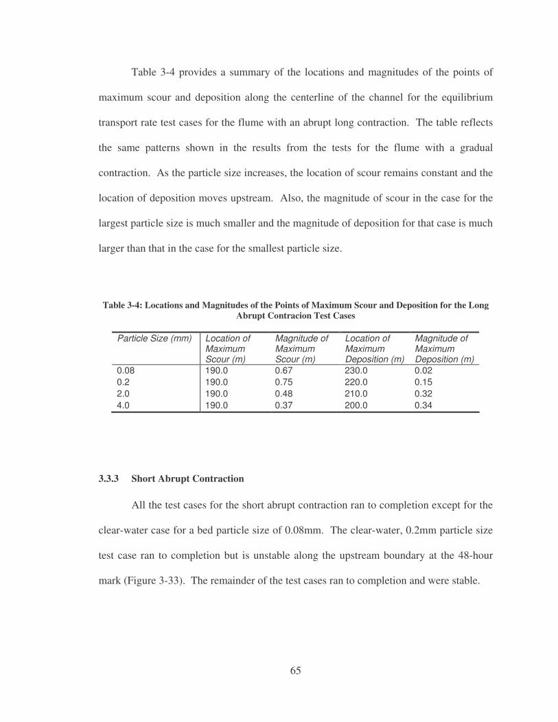
65
Table 3-4 provides a summary of the locations and magnitudes of the points of
maximum scour and deposition along the centerline of the channel for the equilibrium
transport rate test cases for the flume with an abrupt long contraction. The table reflects
the same patterns shown in the results from the tests for the flume with a gradual
contraction. As the particle size increases, the location of scour remains constant and the
location of deposition moves upstream. Also, the magnitude of scour in the case for the
largest particle size is much smaller and the magnitude of deposition for that case is much
larger than that in the case for the smallest particle size.
Table 3-4: Locations and Magnitudes of the Points of Maximum Scour and Deposition for the Long Abrupt Contracion Test Cases
Particle Size (mm) Location of Maximum Scour (m)
Magnitude of Maximum Scour (m)
Location of Maximum Deposition (m)
Magnitude of Maximum Deposition (m)
0.08 190.0 0.67 230.0 0.02 0.2 190.0 0.75 220.0 0.15 2.0 190.0 0.48 210.0 0.32 4.0 190.0 0.37 200.0 0.34
3.3.3 Short Abrupt Contraction
All the test cases for the short abrupt contraction ran to completion except for the
clear-water case for a bed particle size of 0.08mm. The clear-water, 0.2mm particle size
test case ran to completion but is unstable along the upstream boundary at the 48-hour
mark (Figure 3-33). The remainder of the test cases ran to completion and were stable.

66
Figure 3-33: Bed Elevations at 48 Hours for the Clear-Water, 0.2mm Test Case for the Flume with an Abrupt Short contraction, Showing Instability at the Inflow Boundary
The steady-state solution for the water depth shows that the contraction creates a
pool upstream. It also shows that the velocity is quite small upstream (0.27 m/s), rises
dramatically through the contraction, where it peaks at 1.56 m/s, and then falls back
down to 0.5 m/s downstream of the contraction. Longitudinal centerline profiles and plan
views of the steady-state solutions for water depth and velocity magnitude are shown in
the next two figures (Figure 3-34 and Figure 3-35, respectively).
Figure 3-34: Centerline Profile and Plan View of the Steady-State Solution for Water Depth in the Flume with a Short Abrupt Contraction
67
Figure 3-35: Centerline Profile and Plan View of the Steady-State Solution for Velocity Magnitude in the Flume with a Short Abrupt Contraction
The higher velocity that exists through the middle of the channel in the
contraction suggests that the greatest amount of scour will occur in that same area. The
sediment results from FST2DH show that this is accurately reflected by the model run.
Figure 3-36 shows a close-up view of the contraction with an equilibrium transport rate
assigned to the inflow boundary and uniform bed particle sizes of 0.08mm, 0.2mm,
2.0mm, and 4.0mm. The shapes of the regions of scour and deposition seem to be
reasonable.
As was observed in the results from other runs, the results from the short abrupt
contraction test cases showed that as the bed particle size increases, the area of scour
decreases and the area of the deposition moves further upstream, towards the contraction.
The decrease in scour depth is shown in Figure 3-37 with centerline profiles of bed
elevation for increasing particle sizes.

68
Figure 3-36: Bed Elevations after 48 Hours for the Short Abrupt Contraction Flume with an Inflow Equilibrium Transport Rate and Particle Sizes of 0.08mm, 0.2mm, 2.0mm, and 4.0mm
The sediment results from FST2DH also show that, as was observed in the test
cases for the flumes with gradual and long abrupt contractions, the test cases for the short
abrupt contractions have upstream velocities slow enough to eliminate the scour or
deposition of the bed in that region. Therefore, the results from the clear-water test cases
that ran to completion match the results of corresponding test cases with an equilibrium
transport rate assigned to the inflow boundary.
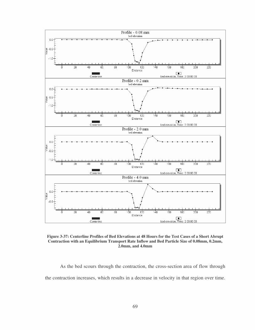
69
Figure 3-37: Centerline Profiles of Bed Elevations at 48 Hours for the Test Cases of a Short Abrupt Contraction with an Equilibrium Transport Rate Inflow and Bed Particle Size of 0.08mm, 0.2mm,
2.0mm, and 4.0mm
As the bed scours through the contraction, the cross-section area of flow through
the contraction increases, which results in a decrease in velocity in that region over time.
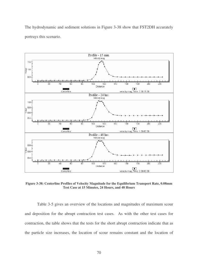
70
The hydrodynamic and sediment solutions in Figure 3-38 show that FST2DH accurately
portrays this scenario.
Figure 3-38: Centerline Profiles of Velocity Magnitude for the Equilibrium Transport Rate, 0.08mm Test Case at 15 Minutes, 24 Hours, and 48 Hours
Table 3-5 gives an overview of the locations and magnitudes of maximum scour
and deposition for the abrupt contraction test cases. As with the other test cases for
contraction, the table shows that the tests for the short abrupt contraction indicate that as
the particle size increases, the location of scour remains constant and the location of
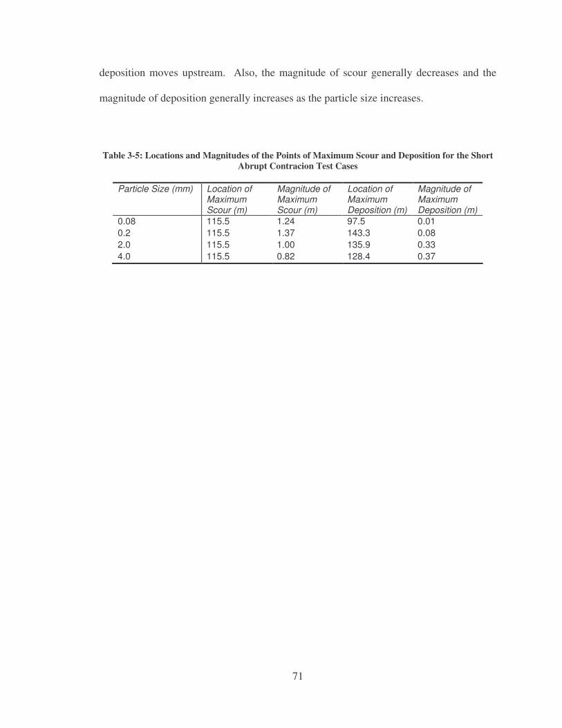
71
deposition moves upstream. Also, the magnitude of scour generally decreases and the
magnitude of deposition generally increases as the particle size increases.
Table 3-5: Locations and Magnitudes of the Points of Maximum Scour and Deposition for the Short Abrupt Contracion Test Cases
Particle Size (mm) Location of Maximum Scour (m)
Magnitude of Maximum Scour (m)
Location of Maximum Deposition (m)
Magnitude of Maximum Deposition (m)
0.08 115.5 1.24 97.5 0.01 0.2 115.5 1.37 143.3 0.08 2.0 115.5 1.00 135.9 0.33 4.0 115.5 0.82 128.4 0.37

72
73
4 Presentation of Results: Quantitative Analysis
The results given in chapter 3 identified the specific sediment transport options
that are currently functional in FST2DH and also examined the degree to which the
results obtained made sense intuitively. This chapter provides comparisons between the
results from FST2DH and those from two other programs, SED2D WES and SAMwin. It
also gives the results from several FST2DH test cases built with data from previous
research with laboratory flumes and comments on those results. The last section in this
chapter reviews the results from an FST2DH simulation modeling the deposition of
sediment at a river’s entrance into a reservoir.
4.1 SED2D WES
The test cases created for the comparison of FST2DH sediment results to those
from SED2D WES provide insight pertaining to the advantages of using a semi-coupled
model instead of an uncoupled one. The results from the test cases also illustrate that the
general patterns seen in the changing bed elevations of an FST2DH sediment simulation
are consistent with those predicted by SED2D WES.
Previous analysis suggested that currently the Ackers-White Formula in FST2DH
does not work appropriately. Because SED2D WES only supports the Ackers-White
Formula (USACE 2004), the simulations were created using different equations for the
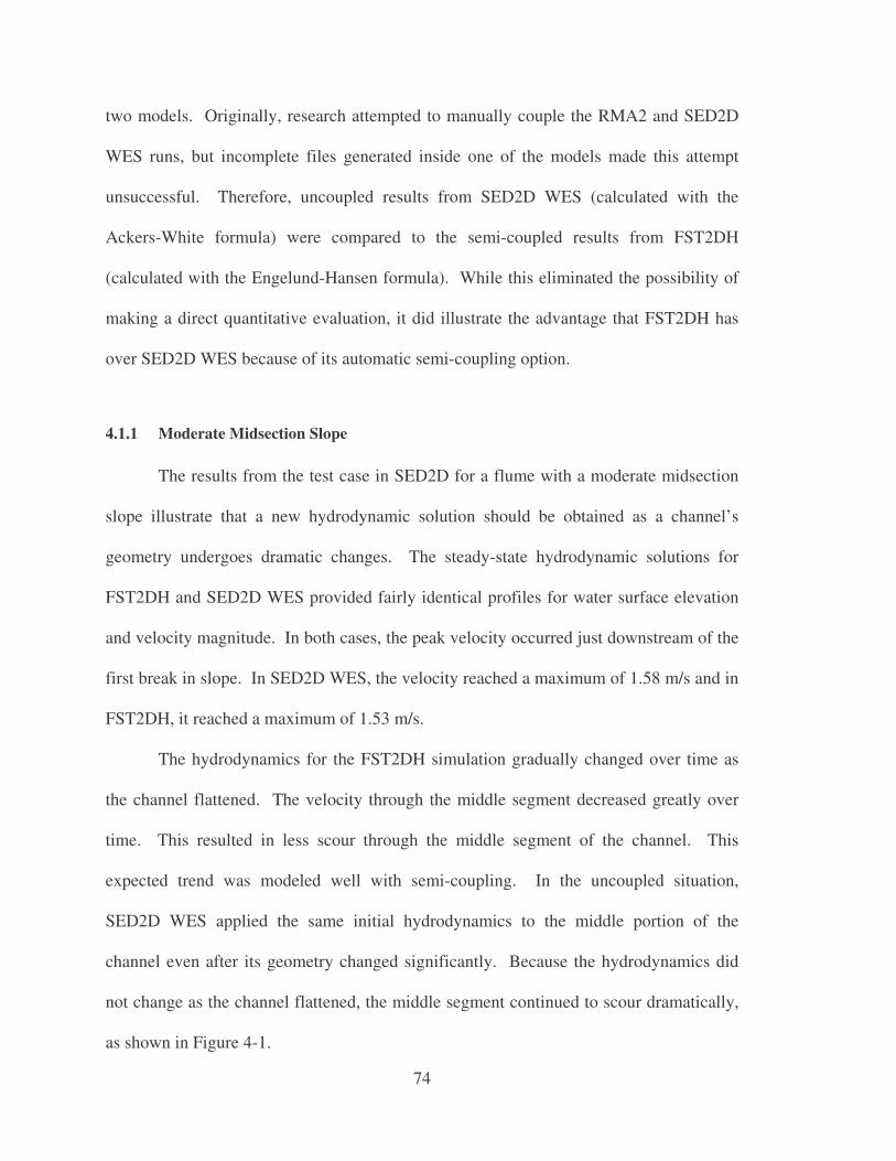
74
two models. Originally, research attempted to manually couple the RMA2 and SED2D
WES runs, but incomplete files generated inside one of the models made this attempt
unsuccessful. Therefore, uncoupled results from SED2D WES (calculated with the
Ackers-White formula) were compared to the semi-coupled results from FST2DH
(calculated with the Engelund-Hansen formula). While this eliminated the possibility of
making a direct quantitative evaluation, it did illustrate the advantage that FST2DH has
over SED2D WES because of its automatic semi-coupling option.
4.1.1 Moderate Midsection Slope
The results from the test case in SED2D for a flume with a moderate midsection
slope illustrate that a new hydrodynamic solution should be obtained as a channel’s
geometry undergoes dramatic changes. The steady-state hydrodynamic solutions for
FST2DH and SED2D WES provided fairly identical profiles for water surface elevation
and velocity magnitude. In both cases, the peak velocity occurred just downstream of the
first break in slope. In SED2D WES, the velocity reached a maximum of 1.58 m/s and in
FST2DH, it reached a maximum of 1.53 m/s.
The hydrodynamics for the FST2DH simulation gradually changed over time as
the channel flattened. The velocity through the middle segment decreased greatly over
time. This resulted in less scour through the middle segment of the channel. This
expected trend was modeled well with semi-coupling. In the uncoupled situation,
SED2D WES applied the same initial hydrodynamics to the middle portion of the
channel even after its geometry changed significantly. Because the hydrodynamics did
not change as the channel flattened, the middle segment continued to scour dramatically,
as shown in Figure 4-1.
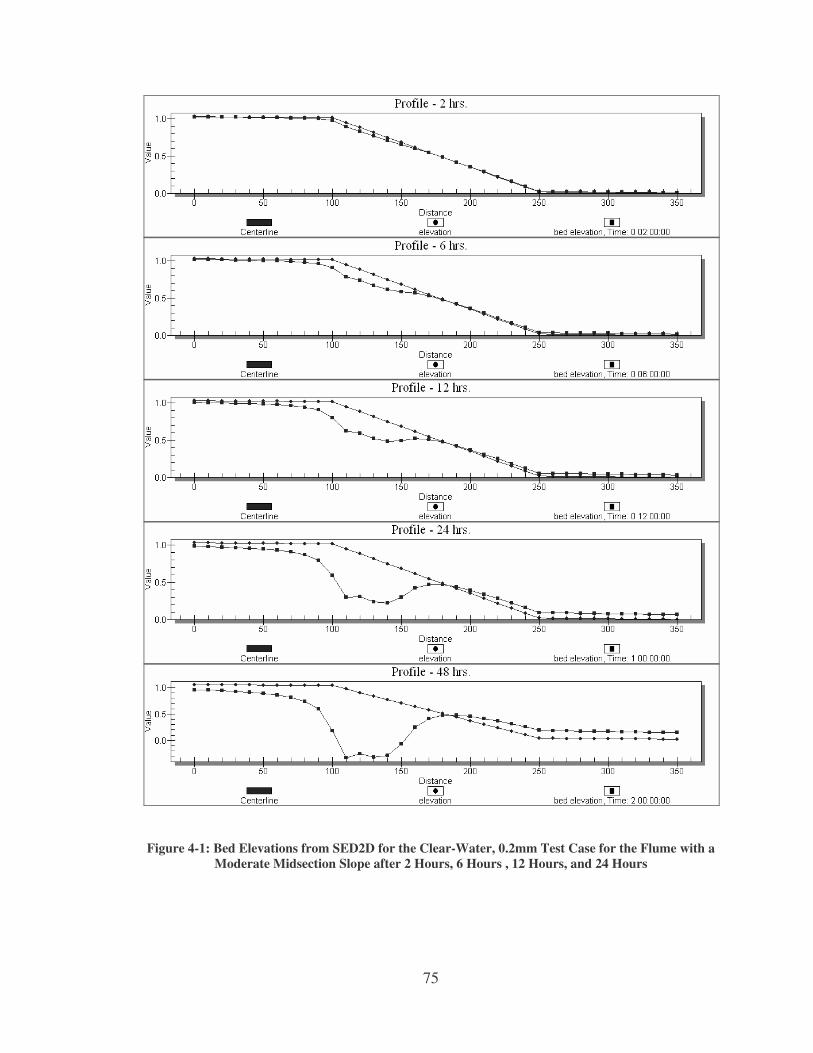
75
Figure 4-1: Bed Elevations from SED2D for the Clear-Water, 0.2mm Test Case for the Flume with a Moderate Midsection Slope after 2 Hours, 6 Hours , 12 Hours, and 24 Hours

76
The final bed from the SED2D run does not reflect scour patterns expected for
this flume. A comparison of the final bed profiles after a 48-hour simulation in FST2DH
and SED2D WES (Figure 4-2) shows that SED2D WES predicted a much different scour
pattern than did FST2DH because of its uncoupled nature. The bed profile found with
FST2DH seems more appropriate for the given case. The figure also shows that the point
separating scour and deposition falls at the same location for both cases—halfway down
the sloped midsection.
Figure 4-2: Final Bed Profiles for SED2D and FST2DH for a 48 Hour Simulation of the Clear-Water, 0.2mm Test Case for the Flume with a Moderate Midsection Slope
4.1.2 Gradual Contraction
The second set of tests created for the comparison of FST2DH and SED2D WES
consisted of simulations for various particle sizes in a flume with a gradual contraction.
77
The steady-state hydrodynamic solutions from SED2D WES and FST2DH were very
similar. When compared to the FST2DH sediment results, the SED2D WES solution for
the 0.08 mm test case showed that when a large amount of scour or deposition occurred
during a simulation, the uncoupled model does not provide appropriate bed elevations.
Figure 4-3 gives the final bed elevations from FST2DH and SED2D WES for this case.
The bed scoured ten times deeper with SED2D WES because the hydrodynamics used in
the sediment calculation didn’t change to reflect the new geometry in the contraction.
Also, SED2D WES did not predict any deposition downstream. These results show that
FST2DH more closely represents the expected scour and deposition than does SED2D
WES. Although an equilibrium transport rate was used in FST2DH and clear water was
used in SED2D, the results from the two cases were comparable because neither scour
nor deposition occurred upstream in either setup, suggesting a state of equilibrium.
Figure 4-3: Final Bed Elevations from FST2DH and SED2D for the 0.08mm Test Case for the Flume with a Gradual Contraction

78
As the sediment size modeled in SED2D WES increased, the bed scoured less
through the contraction (Figure 4-4). FST2DH showed this same pattern and it makes
sense intuitively.
Figure 4-4: Final Bed Elevations from SED2D for the Test Cases for the Flume with a Gradual Contraction with Particle Sizes of 0.08mm, 0.2mm, 2.0mm, and 4.0mm
79
The results from SED2D WES suggest that less scour occurs for larger particle
sizes than FST2DH predicted. There is no documentation that verifies appropriate
implementation or testing of the Ackers-White formula in SED2D WES. The SED2D
WES User’s Manual does, however, state that the appropriateness of its use with the
Ackers-White formula diminishes as the courseness of the modeled sediment increases
(USACE 2004).
Although the results from the SED2D WES test cases don’t provide reasonable
comparison to FST2DH results for a quantitative analysis, they still effectively illustrate
the importance of running hydrodynamic and sediment calculations in a semi-coupled
mode. The tests specifically showed that coupling is a critical part of obtaining an
appropriate solution, especially when the geometry of a channel changes significantly.
Furthermore, the test cases for SED2D WES demonstrated that once all the options for
sediment transport in FST2DH are completely functional, FST2DH will be even more
advantageous over SED2D WES for the modeling of sediment transport because of the
limitations of SED2D WES.
4.2 SAMwin
SAMwin applies sediment transport capacity equations to calculate the sediment
transport capacity of a river that is in general equilibrium (Thomas 2002). When an
equilibrium transport rate is specified for the inflow boundary in an FST2DH model,
FST2DH calculates the concentration of sediment required to create an equilibrium
condition at the inflow boundary so that the amount of sediment entering the model is
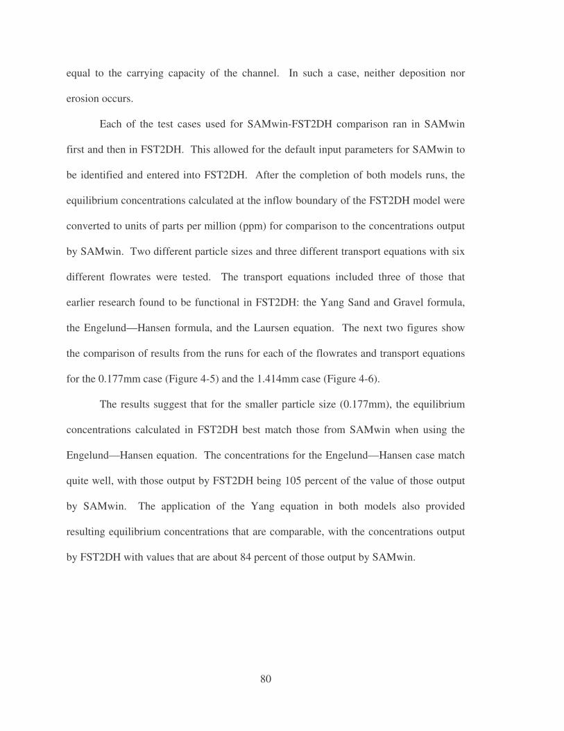
80
equal to the carrying capacity of the channel. In such a case, neither deposition nor
erosion occurs.
Each of the test cases used for SAMwin-FST2DH comparison ran in SAMwin
first and then in FST2DH. This allowed for the default input parameters for SAMwin to
be identified and entered into FST2DH. After the completion of both models runs, the
equilibrium concentrations calculated at the inflow boundary of the FST2DH model were
converted to units of parts per million (ppm) for comparison to the concentrations output
by SAMwin. Two different particle sizes and three different transport equations with six
different flowrates were tested. The transport equations included three of those that
earlier research found to be functional in FST2DH: the Yang Sand and Gravel formula,
the Engelund—Hansen formula, and the Laursen equation. The next two figures show
the comparison of results from the runs for each of the flowrates and transport equations
for the 0.177mm case (Figure 4-5) and the 1.414mm case (Figure 4-6).
The results suggest that for the smaller particle size (0.177mm), the equilibrium
concentrations calculated in FST2DH best match those from SAMwin when using the
Engelund—Hansen equation. The concentrations for the Engelund—Hansen case match
quite well, with those output by FST2DH being 105 percent of the value of those output
by SAMwin. The application of the Yang equation in both models also provided
resulting equilibrium concentrations that are comparable, with the concentrations output
by FST2DH with values that are about 84 percent of those output by SAMwin.

81
Predicted Equilibrium Concentrations (0.177mm)
200
400
600
800
1000
1200
1400
0 2000 4000 6000 8000 10000 12000 14000 16000 18000
Predicted Concentration (ppm)
Flo
wra
te (
cfs)
SAMwin - Yang FST2DH - Yang
SAMwin - Engelund-Hansen FST2DH - Engelund-Hansen
SAMwin - Laursen (Copeland) FST2DH - Laursen
Figure 4-5: Equilibrium Transport Concentrations Predicted by FST2DH and SAMwin for Varying Flowrates and Transport Equations for Test Cases with a 0.177mm Particle Size
Predicted Equilibrium Concentrations (1.414mm)
200
400
600
800
1000
1200
1400
0 200 400 600 800 1000 1200 1400 1600
Predicted Concentration (ppm)
Flo
wra
te (
cfs)
SAMwin - Yang FST2DH - Yang
SAMwin - Engelund-Hansen FST2DH - Engelund-Hansen
SAMwin - Laursen (Copeland) FST2DH - Laursen
Figure 4-6: Equilibrium Transport Concentrations Predicted by FST2DH and SAMwin for Varying Flowrates and Transport Equations for Test Cases with a 1.414mm Particle Size

82
The Laursen (Copeland) equation provided in SAMwin is a modification to the
Laursen equation used in FST2DH, as it extends the applicability of the Laursen equation
to larger gravel sizes (Thomas 2002). Because the grain sizes used in the test cases for
FST2DH and SAMwin are smaller, a reasonable comparison could be made between the
two models using the Laursen and the Laursen (Copeland) formulas. The resulting
equilibrium concentrations from FST2DH (using the Laursen equation) and SAMwin
(using the Laursen (Copeland) formula) provided a relatively poor agreement between
the concentrations output from each model. The concentrations reported by FST2DH for
this case are only 24 percent of those found with SAMwin.
The test cases with the 1.414 mm grain size showed that when larger particles
were used, the tests for the Yang equation provided a closer match for the equilibrium
concentrations output by each model than the Engelund—Hansen formula. The FST2DH
concentrations from models using the Yang Equation fell at about 90 percent of the
values of those predicted by SAMwin with the same equation. With the Engelund—
Hansen equation, FST2DH gave concentrations that were about 76 percent of the value of
those found with SAMwin. The Laursen and Laursen (Copeland) equations again
provided the poorest agreement of concentration, with those calculated by FST2DH being
only 28 percent of the value of those obtained with SAMwin.
The Engelund—Hansen equation appears to be implemented fairly well in
FST2DH. The model does a good job of calculating appropriate equilibrium
concentrations when the Engelund—Hansen equation is used with smaller sediment
sizes. As the sediment size increases, the appropriateness of the application of

83
Engelund—Hansen equation in an FST2DH model decreases and the appropriateness of
Yang’s Sand and Gravel formula increases.
4.3 Laboratory Models
The test cases for the simulation of several different laboratory flumes provided
additional information about the modeling of sediment transport in FST2DH. Research
included the setup for simulations of five different laboratory flumes in FST2DH. Each
of the test cases illustrated that although FST2DH provides logical and intuitive results
for general and hypothetical sediment transport analysis, difficulty arises when specific
laboratory models are to be simulated. Some of the difficulties encountered in this
portion of the research are explained in the next few paragraphs. The sections that follow
provide an overview of the modeling attempts made and possible reasons for their failure.
One of the main difficulties experienced while modeling the small laboratory
flumes in FST2DH was that when the elements represented small areas, the resulting
model runs were unstable. The research enlarged one of the models to determine if
FST2DH would be more stable with elements that represented larger areas and found that
that was the case. Others have experienced similar difficulty in modeling small channels
with elements that represented very small areas (Barton 2001). While a larger-scaled
model of a laboratory flume can be created, doing so may introduce other errors into the
simulation and it would thus not represent the actual conditions in the laboratory.
A second difficulty arose when modeling laboratory flumes in FST2DH because of
the limitations in the current functionality of the sediment transport options in FST2DH.
Most of the laboratory models described in various journal articles included the inflow of
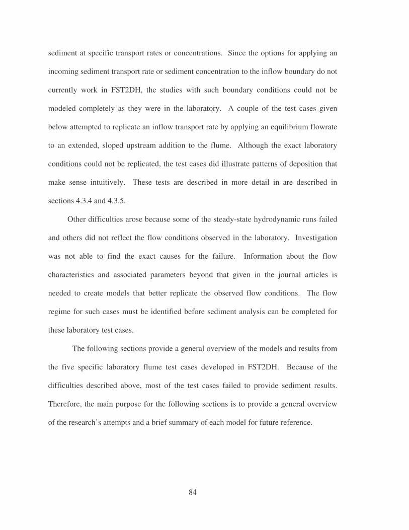
84
sediment at specific transport rates or concentrations. Since the options for applying an
incoming sediment transport rate or sediment concentration to the inflow boundary do not
currently work in FST2DH, the studies with such boundary conditions could not be
modeled completely as they were in the laboratory. A couple of the test cases given
below attempted to replicate an inflow transport rate by applying an equilibrium flowrate
to an extended, sloped upstream addition to the flume. Although the exact laboratory
conditions could not be replicated, the test cases did illustrate patterns of deposition that
make sense intuitively. These tests are described in more detail in are described in
sections 4.3.4 and 4.3.5.
Other difficulties arose because some of the steady-state hydrodynamic runs failed
and others did not reflect the flow conditions observed in the laboratory. Investigation
was not able to find the exact causes for the failure. Information about the flow
characteristics and associated parameters beyond that given in the journal articles is
needed to create models that better replicate the observed flow conditions. The flow
regime for such cases must be identified before sediment analysis can be completed for
these laboratory test cases.
The following sections provide a general overview of the models and results from
the five specific laboratory flume test cases developed in FST2DH. Because of the
difficulties described above, most of the test cases failed to provide sediment results.
Therefore, the main purpose for the following sections is to provide a general overview
of the research’s attempts and a brief summary of each model for future reference.

85
4.3.1 Scour Patterns and Depths Around a Pier
The first laboratory flume test case consisted of an FST2DH model of one the
experiment runs (experiment 10) from a set of clear-water scour tests for flow around
piers of various sizes (Sheppard 2004). The full set of laboratory tests included
representation of three differently-sized piers. Experiment 10 provided analysis of the
scour that occurred around a pier with a diameter of 0.91 meters. Figure 4-7 shows the
grid created for this test case.
Figure 4-7: Grid for Experiment 10 from Sheppard’s Experiments
The steady-state hydrodynamic run for this test case would not run to completion.
Although many attempts were made and the input parameters were all checked for
reasonableness, the steady-state run continued to fail. With the aid of the spin-down
steering option in the Surface-Water Modeling System (SMS), the simulation still only
ran to about 50% completion. The purpose for the failure remains unclear, and a
sediment transport simulation could not be carried forward.
86
4.3.2 Narrow Contraction Flume with Varying Entrance and Exit Angles
A series of laboratory experiments performed by Dey et al. illustrated the
different maximum scour depths that resulted from the variation of the width of a long
contraction (Dey 2005). The widest portion of the flume was 0.6 meters wide and the
entire flume was 12.0 meters long. The journal article provided measurements of
upstream velocity and water depth for each experiment, but only mentioned that the
flume was “tilting” and did not give a specific slope or flowrate. The current research
made several attempts to match the hydrodynamic conditions of the laboratory flume in
FST2DH, but was unsuccessful at doing so. More detail about the specific flowrates and
downstream water surface elevations observed in each of the test cases would be
beneficial. Figure 4-8 shows the grid for the flume with the widest contraction (0.42 m).
Figure 4-8: Grid for Dey’s Experiment for the Flume with the Largest Contraction
4.3.3 Scour at a Basin’s Entrance
Two papers found during the research process referred to experiments completed
by Thuc (Thuc 1991) in which Thuc examined the erosion in a basin due to clear-water
inflow (Duc 2004, Wu 2004). Journal articles by Duc and Wu provided the dimensions

87
for the experimental basin, as well as the velocity for the inflow channel and the water
surface elevation for the outflow channel. The slope was assumed to be zero, based on
the elevations along the beginning and ending segments of the bed elevation curves given
in a plot in Duc’s paper (Duc 2004). Because the papers by Duc and Wu provide no
further information about the flow regime, it remains unknown whether a hydraulic jump
occurred near the basin opening. Without more information about the flow regime, the
research was unable to create a reasonable hydrodynamic solution and the sediment
transport could not be modeled accurately in FST2DH. More specific data needs to be
obtained directly from Thuc’s dissertation (Thuc 1991) before an appropriate model can
be created. Figure 4-9 shows the grid created for Thuc’s Experiment.
Figure 4-9: Grid for Thuc’s Experiment

88
4.3.4 Narrow Flume with Downstream Fining
Seal et al. modeled downstream fining in a long, narrow (0.3 meters wide)
rectangular flume with smooth walls and floor (Seal 1997). A flowrate of 0.049 cms
carried sediment fed to the flume at its upstream end down the flume. Some of the larger
sediment deposited fairly quickly and the smaller sediment was carried further
downstream. Because the option for specifying an inflow sediment concentration or
transport rate in FST2DH does not work properly, a steeper-sloped segment was added to
the upstream end of the modeled flume and an equilibrium transport rate was applied to
the upstream boundary. Manipulation of the slope of the upstream portion attempted to
match the sediment feed rate from the laboratory experiment. While the steady-state
hydrodynamic runs succeeded, each of the sediment runs attempted failed after a few
timesteps. It is believed that the failure resulted from the narrow width of the flume.
Each element only covered a very small area, and in such cases, the model seemed to be
unstable. This reason for failure is supported by the results of the test case described in
the next section, in which a sediment model of a similar, yet wider channel ran
successfully.
4.3.5 Wide Flume with Downstream Fining
Toro-Escobar et al. performed several experiments on downstream fining in flumes
with a width of 2.7 meters (Toro-Escobar 2000). One of their experiments, labeled Run 5
in the Toro-Escobar paper, examined the downstream fining of sandy sediment along the
length of the flume. Similar to Seal’s experiment, Toro-Escobar’s experiment included
an inflow sediment rate, which FST2DH cannot currently replicate appropriately.
Therefore, the model was modified by adding an extension with a slightly steeper slope
89
to the upstream boundary of the model. The inflow boundary’s flowrate and the outflow
boundary’s water surface elevation were set to match the data from the Toro-Escobar
experiment and an equilibrium sediment transport rate was assigned to the inflow
boundary. The bed consisted of a single grain size of 2.0 mm, representing the geometric
mean grain size from the Toro-Escobar paper.
Research adjusted the slope of the upstream segment until a sediment concentration
of approximately 20 kg/min entered the mesh. This rate (two-thirds of that given by
Toro-Escobar et al.) was chosen arbitrarily but still provided results that showed an
appropriate trend. Even if the inflow rate of sediment matched that given in the Toro-
Escobar paper, the resulting bed profile would not be the same as that observed in the
laboratory. This happens because the sediment entering the domain deposits upstream
from the break in slope and thus, less sediment enters the region modeled in the
laboratory.
Figure 4-10 shows the change in the bed over time for the Toro-Escobar test case,
modified slightly due to the limitations in the functionality of the FST2DH sediment
transport options. The pattern of deposition shown in the figure makes sense intuitively.
It begins near the break in slope, where the velocity of the flow slows dramatically. The
volume of deposited material increases throughout the entire simulation and the front of
the zone of deposition gradually moves downstream.

90
Figure 4-10: Bed Elevations for the Modified Toro-Escobar Test Case after 2 Hours, 6 Hours, 12 Hours, 24 Hours, and 32.5 Hours
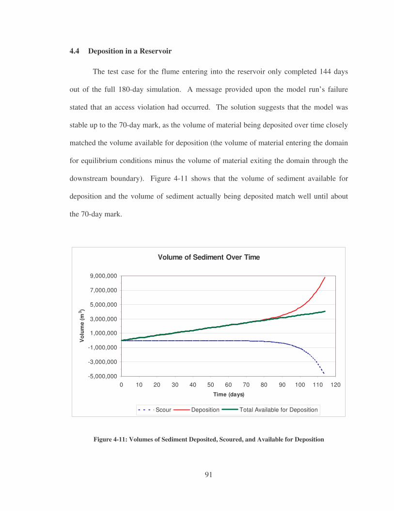
91
4.4 Deposition in a Reservoir
The test case for the flume entering into the reservoir only completed 144 days
out of the full 180-day simulation. A message provided upon the model run’s failure
stated that an access violation had occurred. The solution suggests that the model was
stable up to the 70-day mark, as the volume of material being deposited over time closely
matched the volume available for deposition (the volume of material entering the domain
for equilibrium conditions minus the volume of material exiting the domain through the
downstream boundary). Figure 4-11 shows that the volume of sediment available for
deposition and the volume of sediment actually being deposited match well until about
the 70-day mark.
Volume of Sediment Over Time
-5,000,000
-3,000,000
-1,000,000
1,000,000
3,000,000
5,000,000
7,000,000
9,000,000
0 10 20 30 40 50 60 70 80 90 100 110 120
Time (days)
Vol
ume
(m3 )
Scour Deposition Total Available for Deposition
Figure 4-11: Volumes of Sediment Deposited, Scoured, and Available for Deposition
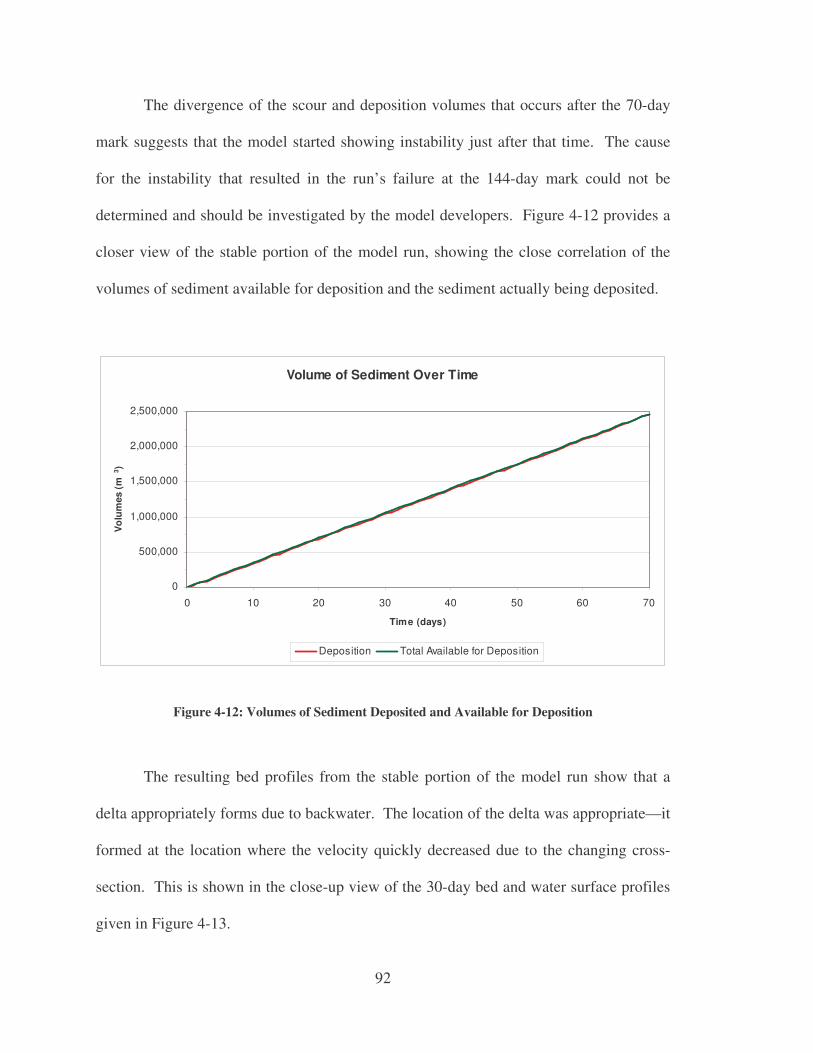
92
The divergence of the scour and deposition volumes that occurs after the 70-day
mark suggests that the model started showing instability just after that time. The cause
for the instability that resulted in the run’s failure at the 144-day mark could not be
determined and should be investigated by the model developers. Figure 4-12 provides a
closer view of the stable portion of the model run, showing the close correlation of the
volumes of sediment available for deposition and the sediment actually being deposited.
Volume of Sediment Over Time
0
500,000
1,000,000
1,500,000
2,000,000
2,500,000
0 10 20 30 40 50 60 70
Time (days)
Vo
lum
es (
m3 )
Deposition Total Available for Deposition
Figure 4-12: Volumes of Sediment Deposited and Available for Deposition
The resulting bed profiles from the stable portion of the model run show that a
delta appropriately forms due to backwater. The location of the delta was appropriate—it
formed at the location where the velocity quickly decreased due to the changing cross-
section. This is shown in the close-up view of the 30-day bed and water surface profiles
given in Figure 4-13.

93
Figure 4-13: Profiles for the Water Surface Elevation, Original Bed Elevations, and Bed Elevations after 30 Days
The delta that formed over time gradually increased in depth and gradually moved
downstream. The steepness of the downstream face of the delta increased as well. This
pattern of aggradation that occurred as a result of a backwater appropriately followed that
described generally by Hotchkiss (1991). Figure 4-14 shows the bed profiles for several
different timesteps from the FST2DH simulation.
Research found that a large amount of material deposited over a relatively short
amount of time. It further discovered that the volumes of sediment available for
deposition (the volume of sediment inflow minus outflow) matched closely with the
volume of sediment deposited for each timestep in the first 70 minutes of simulation. To
verify that the equilibrium inflow concentration calculated by FST2DH was appropriate,
research modeled the upstream portion of the channel in SAMwin. SAMwin gave an
equilibrium concentration of 1,146 ppm. The concentration predicted by FST2DH (1,070
ppm) closely matched that obtained from SAMwin, falling at about 93 percent of its
value (a difference of only 76 ppm). This suggests that correct sediment equilibrium
conditions were calculated in the FST2DH test case. Thus, although it was quite large,
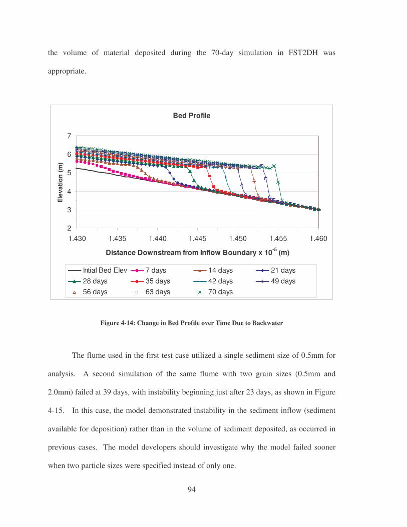
94
the volume of material deposited during the 70-day simulation in FST2DH was
appropriate.
Bed Profile
2
3
4
5
6
7
1.430 1.435 1.440 1.445 1.450 1.455 1.460
Distance Downstream from Inflow Boundary x 10-5 (m)
Ele
vati
on
(m
)
Intial Bed Elev 7 days 14 days 21 days28 days 35 days 42 days 49 days56 days 63 days 70 days
Figure 4-14: Change in Bed Profile over Time Due to Backwater
The flume used in the first test case utilized a single sediment size of 0.5mm for
analysis. A second simulation of the same flume with two grain sizes (0.5mm and
2.0mm) failed at 39 days, with instability beginning just after 23 days, as shown in Figure
4-15. In this case, the model demonstrated instability in the sediment inflow (sediment
available for deposition) rather than in the volume of sediment deposited, as occurred in
previous cases. The model developers should investigate why the model failed sooner
when two particle sizes were specified instead of only one.

95
Volume of Sediment Over Time
0
250,000
500,000
750,000
1,000,000
1,250,000
0 5 10 15 20 25 30 35 40
Time (days)
Vo
lum
es (
m3 )
Deposition Total Available for Deposition
Figure 4-15: Volumes of Deposition and Material Available for Deposition for the Reservoir Test Case with Two Grain Sizes (0.5mm and 2.0mm)
Figure 4-16 shows a plot comparing the resulting bed elevations at 23 days for the
single and multiple grain size simulations.
Bed Profiles (23 days)
3
4
5
6
7
8
140,000 141,000 142,000 143,000 144,000 145,000
Distance Downstream from Inflow Boundary (m)
Ele
vati
on
(m
)
Initial Bed Bed (0.5mm) Bed (0.5mm and 2.0mm)
Figure 4-16: Bed Profiles for the Reservoir Test Case with a Single Grain Size and the Test Case with Two Grain Sizes (0.5mm and 2.0mm)

96
The profiles in Figure 4-16 suggest that deposition occurred furthest upstream in
the test case with two particle sizes. They also show that the delta that formed had a
flatter downstream slope when two particle sizes were specified. The difference in
delta’s location, magnitude, and downstream slope for the two cases results from the fact
that as the river slows down upon entering the zone of backwater, larger sediment stops
moving sooner than smaller sediment comprised of the same type of material (e.g.- sand).
Two of the test cases developed for a longer flume with different element sizes
failed to run to completion (runs C and D). Another test case (run A) showed erosion
throughout the run, which is indicative of other problems in the model, as no scour
should occur in any of the cases. Run B showed an appropriate amount of deposition and
erosion (close to no erosion) and ran to completion. The plots relating the volumes of
material eroded, deposited, and the material available for deposition are shown in the
next four figures (Figure 4-17, Figure 4-18, Figure 4-19, and Figure 4-20). For the two
cases of divergence (run C and run D), the divergence occurred at different times. This
may be due to their different element sizes, but further investigation by model developers
is needed to determine if this is in fact the case. It remains unknown why the volumes for
deposition didn’t match for any of run A. While run B provided some deposition, the
small delta that was formed in the region of backwater did not show up in the bed profile
as being anything more than a small mound, without a steep front edge. A much longer
model run needs to be completed to determine if the delta grows and moves in a manner
similar to that observed in the first test case. However, FST2DH limits the total
allowable simulation time to 9,999 hours (416.6 days), so such a model cannot be created
at the current time.

97
Run A (Element Length = 8696 m)
-500,000
0
500,000
1,000,000
1,500,000
2,000,000
2,500,000
3,000,000
3,500,000
0 50 100 150 200 250 300 350 400
Time (days)
Vo
lum
es (
m3 ) Total Available for
Deposition
Deposition
Erosion
Figure 4-17: Volumes of Erosion, Deposition, and Material Available for Deposition for Run A
Run B (Element Length = 3448 m)
-500,000
0
500,000
1,000,000
1,500,000
2,000,000
2,500,000
3,000,000
3,500,000
0 50 100 150 200 250 300 350 400
Time (days)
Vol
umes
(m3 )
Deposition
Total Available for Deposition
Erosion
Figure 4-18: Volumes of Erosion, Deposition, and Material Available for Deposition for Run B
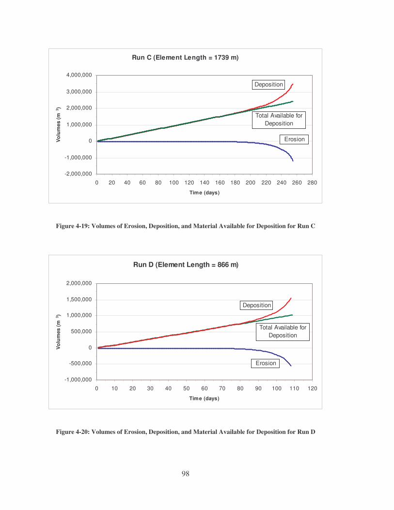
98
Run C (Element Length = 1739 m)
-2,000,000
-1,000,000
0
1,000,000
2,000,000
3,000,000
4,000,000
0 20 40 60 80 100 120 140 160 180 200 220 240 260 280
Time (days)
Vo
lum
es (
m3 )
Deposition
Total Available for Deposition
Erosion
Figure 4-19: Volumes of Erosion, Deposition, and Material Available for Deposition for Run C
Run D (Element Length = 866 m)
-1,000,000
-500,000
0
500,000
1,000,000
1,500,000
2,000,000
0 10 20 30 40 50 60 70 80 90 100 110 120
Time (days)
Vo
lum
es (
m3 )
Deposition
Total Available for Deposition
Erosion
Figure 4-20: Volumes of Erosion, Deposition, and Material Available for Deposition for Run D
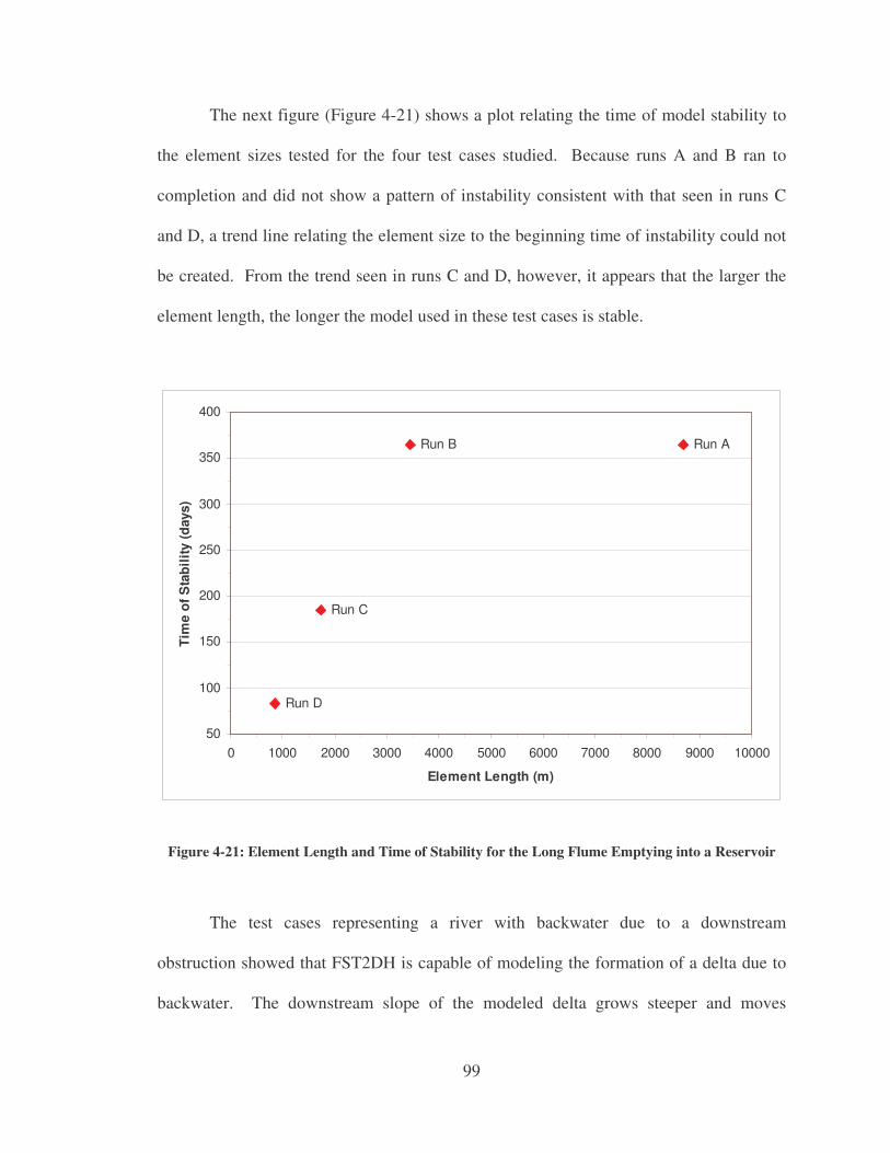
99
The next figure (Figure 4-21) shows a plot relating the time of model stability to
the element sizes tested for the four test cases studied. Because runs A and B ran to
completion and did not show a pattern of instability consistent with that seen in runs C
and D, a trend line relating the element size to the beginning time of instability could not
be created. From the trend seen in runs C and D, however, it appears that the larger the
element length, the longer the model used in these test cases is stable.
Run ARun B
Run C
Run D
50
100
150
200
250
300
350
400
0 1000 2000 3000 4000 5000 6000 7000 8000 9000 10000
Element Length (m)
Tim
e of
Sta
bilit
y (d
ays)
Figure 4-21: Element Length and Time of Stability for the Long Flume Emptying into a Reservoir
The test cases representing a river with backwater due to a downstream
obstruction showed that FST2DH is capable of modeling the formation of a delta due to
backwater. The downstream slope of the modeled delta grows steeper and moves
100
downstream slowly with time, which makes sense intuitively. When two material sizes
are specified, FST2DH shows the formation of a smaller delta further upstream and with
a shallower downstream slope than a delta formed when only a single particle size is
used. Further, the test cases showed that FST2DH has some difficulty in maintaining
stability when modeling sediment movement in large, shallow-sloped models with small
element lengths. It further cannot appropriately simulate sediment transport that occurs
over many years’ time, as it restricts the maximum time of a model run to 9,999 hours
(416.6 days).
101
5 Conclusions
The following sections give an overview of the results of this research and
provide suggestions for possible future research of the sediment transport capabilities of
FST2DH.
5.1 Conclusions
Numerous test cases allowed for the identification of the current functionality of
the sediment transport options in FST2DH. The findings from these tests are given in
section 5.1.1. The other two sections summarize the changes made to SMS to support
FST2DH sediment transport (section 5.1.2) and the suggested changes for the
improvement of the FST2DH sediment transport capabilities (section 5.1.3).
5.1.1 Test Case Results and Observations
Each set of tests included several cases that ran to completion and provided
resulting bed elevations that were reasonable and made sense intuitively. However, every
set of tests also contained at least one case that became unstable and failed. The first set
of tests examined the functionality of each of the sediment inflow options offered by
FST2DH (Table 5-1). Research found that tests using either clear-water or equilibrium
transport rate boundary conditions along the inflow boundary ran to completion and gave
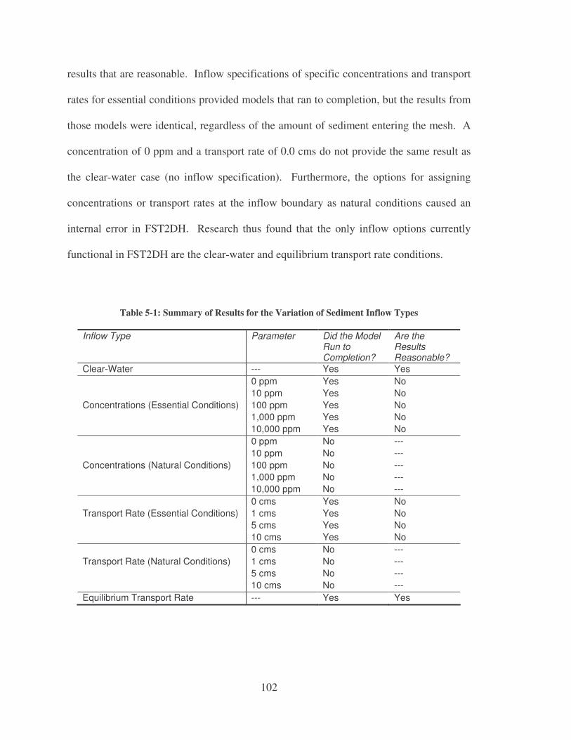
102
results that are reasonable. Inflow specifications of specific concentrations and transport
rates for essential conditions provided models that ran to completion, but the results from
those models were identical, regardless of the amount of sediment entering the mesh. A
concentration of 0 ppm and a transport rate of 0.0 cms do not provide the same result as
the clear-water case (no inflow specification). Furthermore, the options for assigning
concentrations or transport rates at the inflow boundary as natural conditions caused an
internal error in FST2DH. Research thus found that the only inflow options currently
functional in FST2DH are the clear-water and equilibrium transport rate conditions.
Table 5-1: Summary of Results for the Variation of Sediment Inflow Types
Inflow Type Parameter Did the Model Run to Completion?
Are the Results Reasonable?
Clear-Water --- Yes Yes 0 ppm Yes No 10 ppm Yes No Concentrations (Essential Conditions) 100 ppm Yes No 1,000 ppm Yes No 10,000 ppm Yes No 0 ppm No --- 10 ppm No --- Concentrations (Natural Conditions) 100 ppm No ---
1,000 ppm No --- 10,000 ppm No ---
0 cms Yes No Transport Rate (Essential Conditions) 1 cms Yes No 5 cms Yes No 10 cms Yes No
0 cms No --- Transport Rate (Natural Conditions) 1 cms No --- 5 cms No --- 10 cms No --- Equilibrium Transport Rate --- Yes Yes
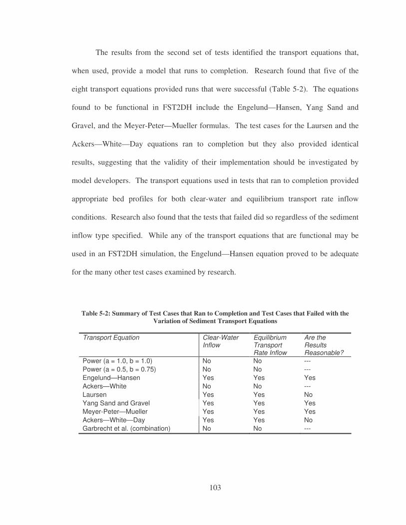
103
The results from the second set of tests identified the transport equations that,
when used, provide a model that runs to completion. Research found that five of the
eight transport equations provided runs that were successful (Table 5-2). The equations
found to be functional in FST2DH include the Engelund—Hansen, Yang Sand and
Gravel, and the Meyer-Peter—Mueller formulas. The test cases for the Laursen and the
Ackers—White—Day equations ran to completion but they also provided identical
results, suggesting that the validity of their implementation should be investigated by
model developers. The transport equations used in tests that ran to completion provided
appropriate bed profiles for both clear-water and equilibrium transport rate inflow
conditions. Research also found that the tests that failed did so regardless of the sediment
inflow type specified. While any of the transport equations that are functional may be
used in an FST2DH simulation, the Engelund—Hansen equation proved to be adequate
for the many other test cases examined by research.
Table 5-2: Summary of Test Cases that Ran to Completion and Test Cases that Failed with the Variation of Sediment Transport Equations
Transport Equation Clear-Water Inflow
Equilibrium Transport Rate Inflow
Are the Results Reasonable?
Power (a = 1.0, b = 1.0) No No --- Power (a = 0.5, b = 0.75) No No --- Engelund—Hansen Yes Yes Yes Ackers—White No No --- Laursen Yes Yes No Yang Sand and Gravel Yes Yes Yes Meyer-Peter—Mueller Yes Yes Yes Ackers—White—Day Yes Yes No Garbrecht et al. (combination) No No ---
104
The third set of test cases used in the examination of the functionality of sediment
transport in FST2DH included channels with varying midsection slopes and contractions.
Table 5-3 gives a summary of the test cases that failed and the ones that ran to
completion. All tests that ran successfully provided reasonable results that were intuitive.
They appropriately defined the location and magnitude of both scour and deposition over
time.
Successful runs showed several expected trends. As the particle size in each case
increased, the amount of scour and deposition in the channel generally decreased and the
deposition occurred further upstream. Cases with an equilibrium transport rate assigned
to the inflow boundary appropriately showed that the bed elevations at the inflow
boundary remained constant over time. All successful tests showed scouring in areas of
higher velocity and deposition in areas where the water slowed down. Another trend
observed by research was that the hydrodynamic solution changed as the geometry of the
channel changed with scour and deposition over time. Specifically, as the bed scoured,
the solution showed an increase in water depth and a decrease in velocity. Over time, as
the highest velocities in the channel decreased, less sediment movement occurred. These
trends suggest that the semi-coupling mode in FST2DH works appropriately.
FST2DH was unstable when small particle sizes (fine sand) where used for the
clear-water inflow condition. The equilibrium inflow condition proved to provide more
stability. Instability also occurred for all test cases run on the channel with a steep
midsection slope. Research found that instability also occurred in the region of the
hydraulic jump modeled in the test cases for the channel with a steep midsection slope.
The complex flow and energy conditions associated with hydraulic jumps most likely

105
caused that instability. The causes for the instability observed in each of the test cases
should be investigated by model developers.
Table 5-3: Identification of the Midsection Sloped and Contraction Test Cases that Ran to Completion and Test Cases that Failed
Channel Sediment Inflow
0.08 mm Particle Size
0.2 mm Particle Size
2.0 mm Particle Size
4.0 mm Particle Size
Steep Midsection Slope Clear-Water No No No No Equilibrium No No No No Moderate Midsection Slope Clear-Water No Yes No No Equilibrium Yes Yes Yes Yes Shallow Midsection Slope Clear-Water No Yes Yes Yes Equilibrium Yes Yes Yes Yes Gradual Contraction Clear-Water No No Yes Yes Equilibrium Yes Yes Yes Yes Long Abrupt Contraction Clear-Water No No Yes Yes Equilibrium Yes Yes Yes Yes Short Abrupt Contraction Clear-Water No Yes Yes Yes Equilibrium Yes Yes Yes Yes
Comparison of FST2DH sediment results to those from SED2D WES illustrated
that semi-coupling is essential for obtaining an appropriate sediment solution when large
changes in the channel geometry occur. Without semi-coupling, the SED2D WES results
did not make sense and didn’t reflect the effects that the change in geometry would have
on the flow condition and vice-versa. Thus, FST2DH results could not really be
compared to those from SED2D WES. However, a couple of similar trends were
observed in the results from each model. Both models predicted similar shapes and
locations of scour and deposition in the flume with a gradual contraction. The results
also showed that for both models, as the particle size increased, the depth of the scour
106
generally decreased. Finally, results from the SED2D WES test cases illustrated several
advantages that FST2DH currently has over SED2D WES, including the following:
• Semi-coupling of hydrodynamic and sediment calculations
• Choice of several transport capacity equations
• Ability to model larger particle sizes, such as gravels
• Ability to model equilibrium sediment inflow transport rate with ease
The equilibrium concentrations calculated with FST2DH for the Engelund—
Hansen equation and the Yang formula match closely with those found with the same two
equations in SAMwin. The concentrations calculated by the two programs for models
with smaller particle sizes matched better when the Engelund—Hansen equation was
used and concentrations calculated for models with larger particle sizes matched better
with the application of the Yang equation.
The laboratory flume test cases illustrated that FST2DH has some difficulty in
modeling laboratory flumes. Table 5-4 provides the results from the several models
created for different laboratory flumes and for the formation of a delta due to backwater
as a river enters a reservoir. One of the difficulties listed in the table for some of the
experiments is that of obtaining stability for models of narrow channels. FST2DH seems
to have more difficulty running models with elements representing small areas than it
does in running models with larger elements. Another difficulty listed in the table is that
of accurately representing conditions seen in the laboratory because of the limited
functionality of the sediment options in FST2DH. Research generally found that the
instabilities encountered with some of the models require users to spend unnecessary
effort and time manipulating the model to make it work.
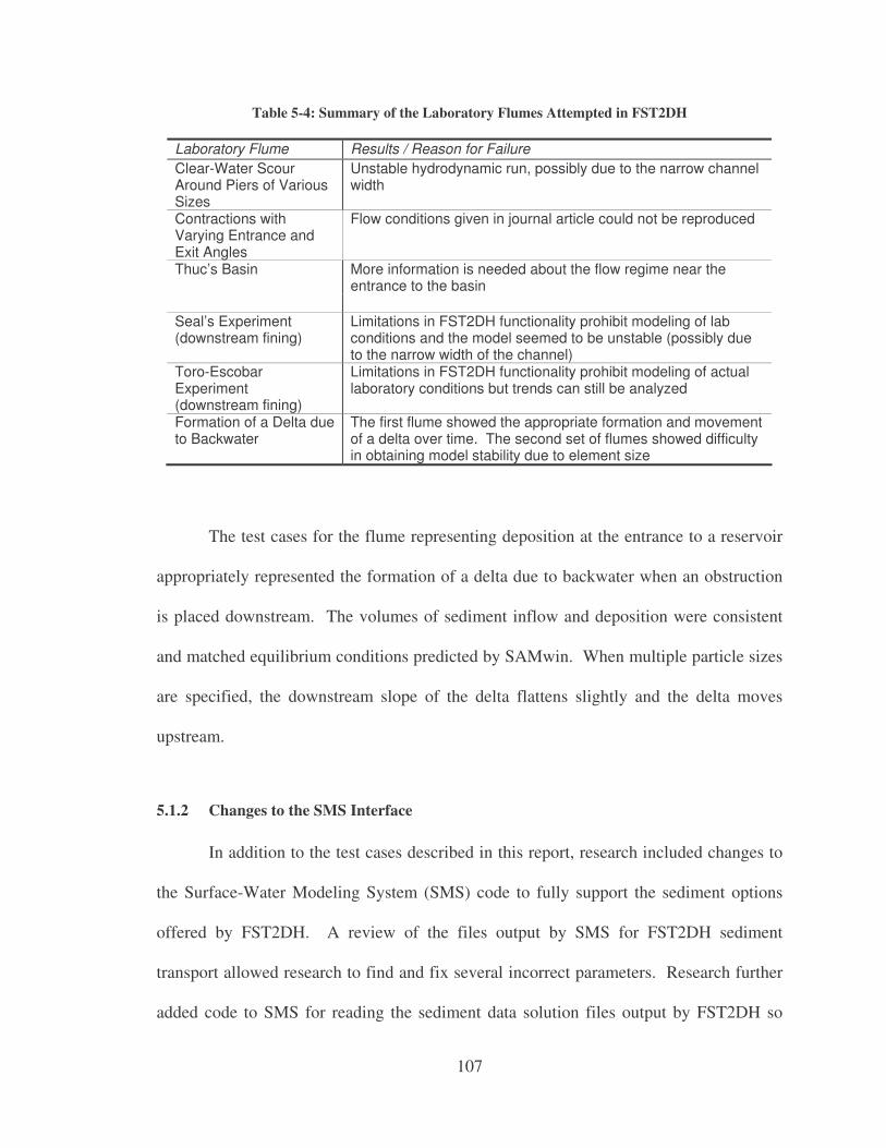
107
Table 5-4: Summary of the Laboratory Flumes Attempted in FST2DH
Laboratory Flume Results / Reason for Failure Clear-Water Scour Around Piers of Various Sizes
Unstable hydrodynamic run, possibly due to the narrow channel width
Contractions with Varying Entrance and Exit Angles
Flow conditions given in journal article could not be reproduced
Thuc’s Basin More information is needed about the flow regime near the entrance to the basin
Seal’s Experiment (downstream fining)
Limitations in FST2DH functionality prohibit modeling of lab conditions and the model seemed to be unstable (possibly due to the narrow width of the channel)
Toro-Escobar Experiment (downstream fining)
Limitations in FST2DH functionality prohibit modeling of actual laboratory conditions but trends can still be analyzed
Formation of a Delta due to Backwater
The first flume showed the appropriate formation and movement of a delta over time. The second set of flumes showed difficulty in obtaining model stability due to element size
The test cases for the flume representing deposition at the entrance to a reservoir
appropriately represented the formation of a delta due to backwater when an obstruction
is placed downstream. The volumes of sediment inflow and deposition were consistent
and matched equilibrium conditions predicted by SAMwin. When multiple particle sizes
are specified, the downstream slope of the delta flattens slightly and the delta moves
upstream.
5.1.2 Changes to the SMS Interface
In addition to the test cases described in this report, research included changes to
the Surface-Water Modeling System (SMS) code to fully support the sediment options
offered by FST2DH. A review of the files output by SMS for FST2DH sediment
transport allowed research to find and fix several incorrect parameters. Research further
added code to SMS for reading the sediment data solution files output by FST2DH so

108
that the sediment results could be analyzed inside SMS. Finally, research involved the
creation of a tutorial that outlines the steps for setting up and running an FST2DH
sediment simulation. The tutorial is included in the appendix of this report.
5.1.3 Suggested Improvements for FST2DH
While many of the sediment options offered by FST2DH are functional, many
options should be fixed. FST2DH developers should examine the algorithms used in
modeling inflow concentrations and flowrates. The implementation of the Power
equation, the Ackers—White equation, and Garbrecht et al. approach should be reviewed
and code should be changed to provide model stability for these cases. Other changes
should be implemented to make FST2DH more stable for models with smaller particle
sizes, hydraulic jumps, and small element sizes.
5.2 Future Work
In order to verify that the sediment transport options in FST2DH work
appropriately after the suggested changes are made to the source code, the test cases that
failed in this research should be run again in FST2DH. Results from those runs should be
evaluated again for reasonableness and to see if they follow the trends established by the
results presented in this report. Additional models that represent simple changes in
geometry should also be evaluated. Furthermore, after research was completed,
investigation of the power equation suggested that the values used in that equation
provided an unfair evaluation of the formula’s functionality (solid sediment flow is
represented when a = 1.0). The power equation should thus be reevaluated using smaller
values for its “a” coefficient once changes are made to the FST2DH code.

109
Because the scope of this thesis involved the identification of the general
functionality of the FST2DH sediment transport options, research has only examined
simple test cases. As model developers fix the faulty sediment transport options in
FST2DH, more complex analysis should be completed to determine the full extent of the
model’s applicability. This analysis would include models of hypothetical and laboratory
flumes, as well as models of real rivers. Examples of hypothetical models may include s-
shaped flumes, flumes with strings of differing contractions and changes in bed, and
flumes with complex cross-sections. Examples of laboratory flumes may include those
given in this report, those found by the current research and not detailed in this report,
and many others (see, for example, Gaudio 2003, Lim 1997, and Yanmaz 1991).
Currently, sediment data files are output by FST2DH in ASCII format. This
results in output files that require a lot of memory and take a lot of time to open in SMS.
Future work may include modification to FST2DH and SMS to write and read sediment
solution files in a compressed XMDF format, which requires less memory and decreases
the amount of time required to read the file into SMS for post-processing.
A final recommendation for future work involves the creation of a standard suite
of tests to be used in the verification process of newly-developed sediment transport
models. The suite would include all data and results from several different laboratory
and field studies that are required for a sediment transport simulation. The hypothetical
models contained in this report may also be included in that suite. Such a collection of
tests would not only benefit further research of sediment transport in FST2DH, but would
also benefit developers of other transport models.

110
111
References
Barton, C. L. (2001). “Flow Through an Abrupt Constriction – 2D Hydrodynamic Model Performance and Influence of Spatial Resolution.” Master’s Thesis, Griffith University, School of Environmental Engineering.
Brush, L. M., Jr. and Wolman, M. G. (1960). “Knickpoint Behavior in Noncohesive
Material: A Laboratory Study.” Bulletin of the Geological Society of America. Volume 41, pp. 59-74.
Cancino, L. and Neves, R. (1999). “Hydrodynamic and Sediment Suspension Modelling
in Estuarine Systems, Part I: Description of the Numerical Models.” Journal of Marine Systems. Volume 22, pp. 105-116.
Chang, H. H. Fluvial Processes in River Engineering. Malabar, FL: Krieger, 1992. Dey, S. and Raikar, R. V. (2005). “Scour in Long Contractions.” Journal of Hydraulic
Engineering, ASCE, Volume 131, Issue 12, pp. 1036-1049. Duc, B. M., Wenka, T., and Rodi, W. (2004). “Numerical Modeling of Bed Deformation
in Laboratory Channels.” Journal of Hydraulic Engineering. Volume 130, Issue 9, pp. 894-904.
Froehlich, D. C. (2003). “User’s Manual for FESWMS FST2DH, Two-dimensional
Depth-averaged Flow and Sediment Transport Model.” U.S. Department of Transportation, Federal Highway Administration, McLean, Virginia.
Gaudio, R. and Marion, A. (2003). “Time Evolution of Scouring Downstream of Bed
Sills.” Journal of Hydraulic Research. Volume 41, Number 3, pp. 271-284. Hotchkiss, R. H. and Parker, G. (1991). “Shock Fitting of Aggradational Profiles Due to
Backwater.” Journal of Hydraulic Engineering. Volume 117, Issue 9, pp. 1129-1144.
Kassem, A. A. and Chaudhry, M. H. (1998). “Comparison of Coupled and Semicoupled
Numerical Models for Alluvial Channels.” Journal of Hydraulic Engineering. Volume 124, Issue 8, pp. 794-802.
112
Lagasse, P. F., Zevenbergen, L. W., Schall, J. D., and Clopper, P. E. (2001). “Bridge Scour and Stream Instability Countermeasures: Experience, Selection and Design Guidance, Second Edition.” U.S. Department of Transportation, Federal Highway Administration, National Highway Institute, Arlington, Virginia.
Lim, S-Y (1997). “Equilibrium Clear-Water Scour Around An Abutment.” Journal of
Hydraulic Engineering. Volume 123, Issue 3, pp. 237-243. Molinas, A. (2000). “User’s Manual for BRI-STARS (Bridge Stream Tube Model for
Alluvial River Simulation).” U.S. Department of Transportatioin, Federal Highway Administration, McLean, Virginia.
Nakato, T. (1990). “Tests of Selected Sediment-Transport Formulas.” Journal of
Hydraulic Engineering. Volume 116, Issue 3, pp. 362-379. Richardson, E. V., Simons, D. B., and Lagasse, P. F. (2001). “River Engineering for
Highway Encroachments: Highways in the River Environment, Hydraulic Design Series Number 6.” U.S. Department of Transportation, Federal Highway Administration, National Highway Institute, Arlington, Virginia.
Seal, R., Paola, C., Parker, G., Southard, J. B., and Wilcock, P. R. (1997). “Experiments
on Downstream Fining of Gravel: I. Narrow-Channel Runs.” Journal of Hydraulic Engineering. Volume 123, Issue 10, pp. 874-884.
Shams, M., Ahmadi, G., and Smith, D. H. (2002). “Computational Modeling of Flow and
Sediment Transport and Deposition in Meandering Rivers.” Advances in Water Resources. Volume 25, pp. 689-699.
Sheppard, D. M., Odeh, M., and Glasser, T. (2004). “Large Scale Clear-Water Local Pier
Scour Experiments.” Journal of Hydraulic Engineering. Volume 130, Issue 10, pp. 957-963.
Thomas, W. A., Copeland, R. R., and McComas, D. N. (2002). “SAM Hydraulic Design
Package for Channels.” U.S. Army Corps of Engineers, Engineer Research and Development Center, Coastal and Hydraulics Laboratory, Vicksburg, Mississippi.
Thuc, T. (1991). “Two-dimensional morphological computations near hydraulic
structures.” Doctoral dissertation. Asian Institute of Technology, Bangkok, Thailand.
Toro-Escobar, C. M., Paola, C., Parker, G., Wilcock, P. R., and Southard, J. B. (2000).
“Experiments on Downstream Fining of Gravel. II: Wide and Sandy Runs.” Journal of Hydraulic Engineering, Volume 126, Issue 3, pp. 198-208.

113
U.S. Army Corps of Engineers (USACE), (2004). “User’s Guide to SED2D WES
Version 4.5.” U.S. Army Corps of Engineers, Engineer Research and Development Center, Waterways Experiment Station, Coastal and Hydraulics Laboratory, Vicksburg, Mississippi.
U.S. Army Corps of Engineers (USACE), (1991). “HEC-6, Scour and Decomposition in
Rivers and Reservoirs, User’s Manual.” U.S. Army Corps of Engineers, Hydrologic Engineering Center, Davis, California.
Wu, W. (2004). “Depth-Averaged Two-Dimensional Numerical Modeling of Unsteady
Flow and Nonuniform Sediment Transport in Open Channels.” Journal of Hydraulic Engineering, Volume 130, Issue 10, pp. 1013-1024.
Yang, C. T., Simões, F. J. M., Huang, J., and Greimann, B. (2005). “Generalized
Sediment Transport Models for Alluvial Rivers and Reservoirs.” US-China Workshop on Advanced Computational Modelling in Hydroscience & Engineering. September 19-21, Oxford, Mississippi, U.S.A.
Yang, C. T. and Wan, S. (1991). “Comparisons of Selected Bed-Material Load
Formulas.” Journal of Hydraulic Engineering. Volume 117, Issue 8, pp. 973-989. Yanmaz, A. M. and Altmbilek, H. D. (1991). “Study of Time-Dependent Local Scour
Around Bridge Piers.” Journal of Hydraulic Engineering. Volume 117, Issue 10, pp. 1247-1268.
Zeng, W., and Beck, M. B. (2003). “STAND, A Dynamic Model for Sediment Transport
and Water Quality.” Journal of Hydrology. Volume 277, Issues 1-2, pp. 125-133.

114
115
Appendix A. FST2DH Sediment Transport Tutorial
The research outlined in this report included changes to the Surface-Water
Modeling System (SMS) software package source code to enable users to set up a
FST2DH sediment run and graphically view and analyze the simulation’s results within
the SMS interface. As part of that update, a new tutorial was created to teach SMS users
how to set up and run a basic FST2DH sediment analysis in SMS. The pages that follow
contain that tutorial.
Introduction
In this lesson you will learn how to set up and run a sediment transport simulation
in FST2DH. The run will be semi-coupled, meaning that once a steady-state
hydrodynamic solution is obtained, sediment and hydrodynamic calculations will be
completed iteratively for all timesteps in the simulation.
Because the sediment transport options in FST2DH are fairly new, some of the
options are not yet fully functional. Information about the current functionality of
specific options can be found in the report accompanying this tutorial.
The first part of this tutorial outlines the setup for a steady-state hydrodynamic
run and the remainder of the tutorial focuses on setting up, running, and interpreting
results for a semi-coupled sediment run. Because FST2DH only supports the non-
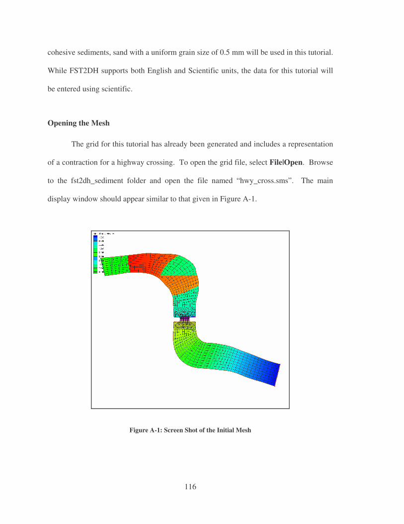
116
cohesive sediments, sand with a uniform grain size of 0.5 mm will be used in this tutorial.
While FST2DH supports both English and Scientific units, the data for this tutorial will
be entered using scientific.
Opening the Mesh
The grid for this tutorial has already been generated and includes a representation
of a contraction for a highway crossing. To open the grid file, select File|Open. Browse
to the fst2dh_sediment folder and open the file named “hwy_cross.sms”. The main
display window should appear similar to that given in Figure A-1.
Figure A-1: Screen Shot of the Initial Mesh
117
Assigning Boundary Conditions
The channel you are modeling will have a flowrate of 60.0 cms and a downstream
water surface elevation of 1.7 m, representing a depth of that same magnitude. To assign
these boundary conditions:
1. Click on the “Select Nodestring” tool.
2. Select the nodestring representing the inflow boundary, located to the lower right
hand end of the mesh.
3. Select FESWMS | Assign BC…
4. Check the Flow toggle, enter a flowrate of 60.0 (cms), and click OK.
5. Select the nodestring representing the outflow boundary, located at the upper left
hand corner of the mesh.
6. Open the boundary conditions dialog again (FESWMS|Assign BC…) and select
the Water surface elevation toggle.
7. Specify a constant water surface elevation (WSE) of 1.7 (m) and click OK to exit
the dialog.
Material Properties
For simplicity, the channel being modeled in this tutorial contains a single
material type—sand. To assign a Manning’s n value for sand to the entire mesh:
1. Select FESWMS | Material Properties…
2. Assign a value of 0.025 for Manning’s roughness (n1 and n2)
3. Click OK to exit the FESWMS Material Properties dialog.
118
Model Control
Most of the parameters used as input for FST2DH simulations are defined in the
FESWMS Model Control dialog. To set up the parameters for a steady-state
hydrodynamic simulation:
1. Select FESWMS | Model Control…
2. In the FESWMS Model Control dialog, select the General Tab, make sure the
Run Type is set to “Hydrodynamic” and the Solution Type is set to “Steady
State”.
3. Select the Timing Tab and set the number of Iterations to 10.
4. Select the Parameters Tab. Assign the Water-surface elevation a value of 1.7
(m), and the Unit flow convergence and Water depth convergence a value of
0.01.
5. Select OK to exit the FESWMS Model Control.
Renumbering the Mesh
Before a hydrodynamic solution is run, the mesh should be renumbered. To
renumber the mesh:
1. Click the “Select Nodestring” tool and select the inflow boundary (at the
lower right end of the mesh).
2. Select Nodestrings | Renumber…
Obtaining the Steady-State Hydrodynamic Solution
Before running FST2DH, you will need to save the file:
119
1. Select File|Save As…
2. Browse to the “fst2dh_sediment\output” folder and save the project file (*.sms) as
“hwy_cross_out.sms”.
Now that the parameters for the steady-state hydrodynamic run have been saved,
you are ready to run FST2DH. Select FESWMS | Run FST2DH to start the simulation.
The model will take a few seconds to run. Once it is complete, make sure the “Load
solution” toggle box is checked and click on the Exit button. The steady-state
hydrodynamic solution opens in SMS.
Some models require the use of incremental loading in order to reach a solution.
In those cases, the hydrodynamic solution serves as a hotstart file for a subsequent semi-
coupled hydrodynamic and sediment simulation. Although the channel in this tutorial did
not require incremental loading, the hydrodynamic solution will still be used as a hotstart
for the semi-coupled simulation so that you can see how it is done.
Creating a Sediment Simulation
You are now ready to set up the sediment simulation. In order to use the
hydrodynamic solution just created by FST2DH as a hotstart for the sediment run, you
must rename the project so the new hydrodynamic output file does not overwrite the
steady-state one. To save the project with a different name:
1. Select File | Save As…
2. Change the File name to “hwy_cross_sed_out.sms” and click Save.

120
Setting the Sediment Parameters in Model Control
You will now set up the appropriate options for the sediment transport simulation.
As was the case for the hydrodynamic run, most of the sediment parameters will be set in
the FESWMS Model Control dialog. To set the parameters:
1. Select FESWMS | Model Control
2. In the General Tab, change the Run Type to “Semi-coupled” to tell FST2DH to
run the hydrodynamic and sediment calculations iteratively for each timestep.
3. Change the Solution Type to “Dynamic” to have FST2DH simulate the
movement of sediment over time
4. Select the Sediment Transport Solutions toggle, click the file macro, and enter
“hwy_cross_sed_out.sed” for the name of the sediment data output file to be
created by FST2DH during the sediment simulation. Click Save.
5. Select the INI file toggle in the FST2DH Input section of the General Tab, click
the file macro, and open the file called “hwy_cross_out.flo” from the
fst2dh_sediment\output folder. This tells FST2DH that the output file from the
steady-state hydrodynamic run will be used as a hotstart for the sediment
simulation.
6. Select the Timing Tab in the FESWMS Model Control dialog. Set the Starting
time to 0.0 (hours), the Run time to 48.0 (hours), and the Time step size to 0.25
(hours). The simulation will run for 48 hours, with a 15-minute timestep.
7. Select the Sediment Control Tab. In this tab, you enter the sediment parameters
for the model run. The options in the Report Options section allow you to
specify which information is included in the *.prt informational text file output by
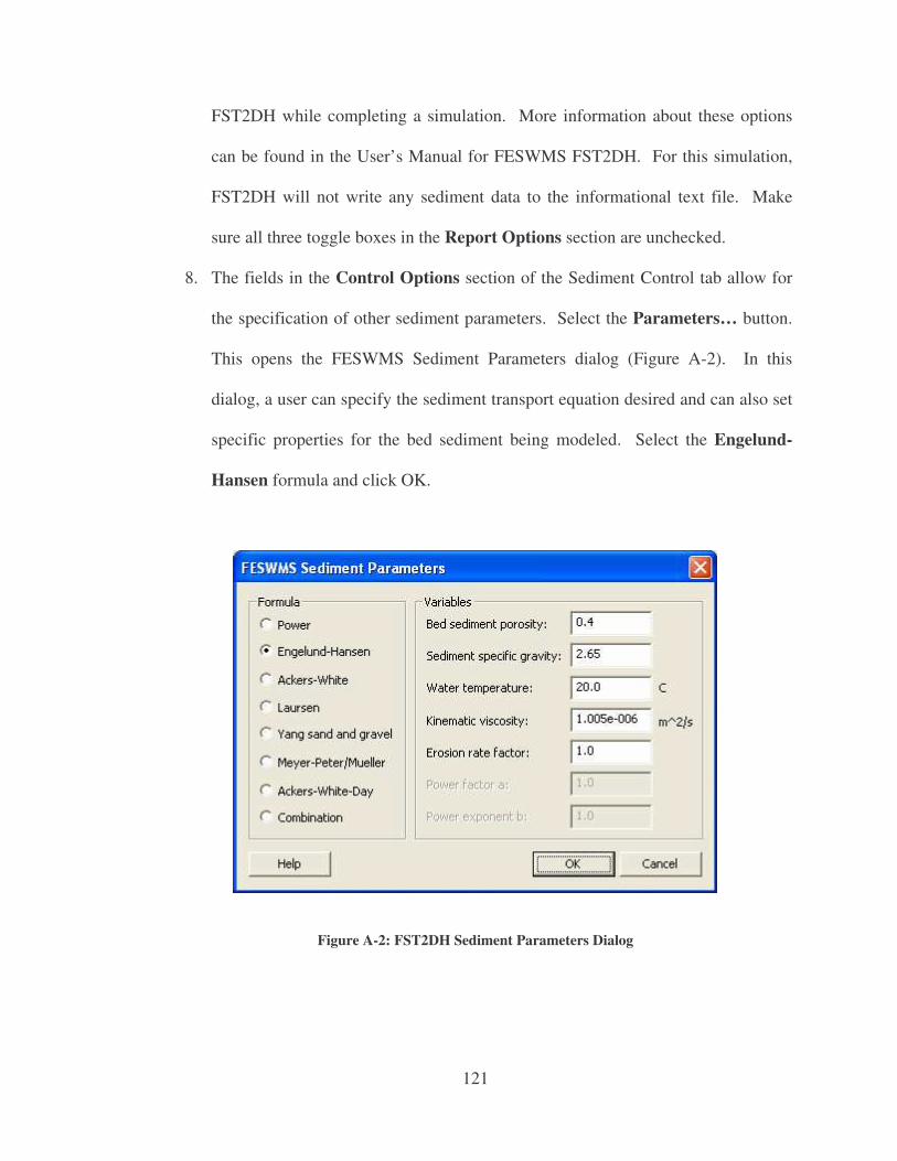
121
FST2DH while completing a simulation. More information about these options
can be found in the User’s Manual for FESWMS FST2DH. For this simulation,
FST2DH will not write any sediment data to the informational text file. Make
sure all three toggle boxes in the Report Options section are unchecked.
8. The fields in the Control Options section of the Sediment Control tab allow for
the specification of other sediment parameters. Select the Parameters… button.
This opens the FESWMS Sediment Parameters dialog (Figure A-2). In this
dialog, a user can specify the sediment transport equation desired and can also set
specific properties for the bed sediment being modeled. Select the Engelund-
Hansen formula and click OK.
Figure A-2: FST2DH Sediment Parameters Dialog
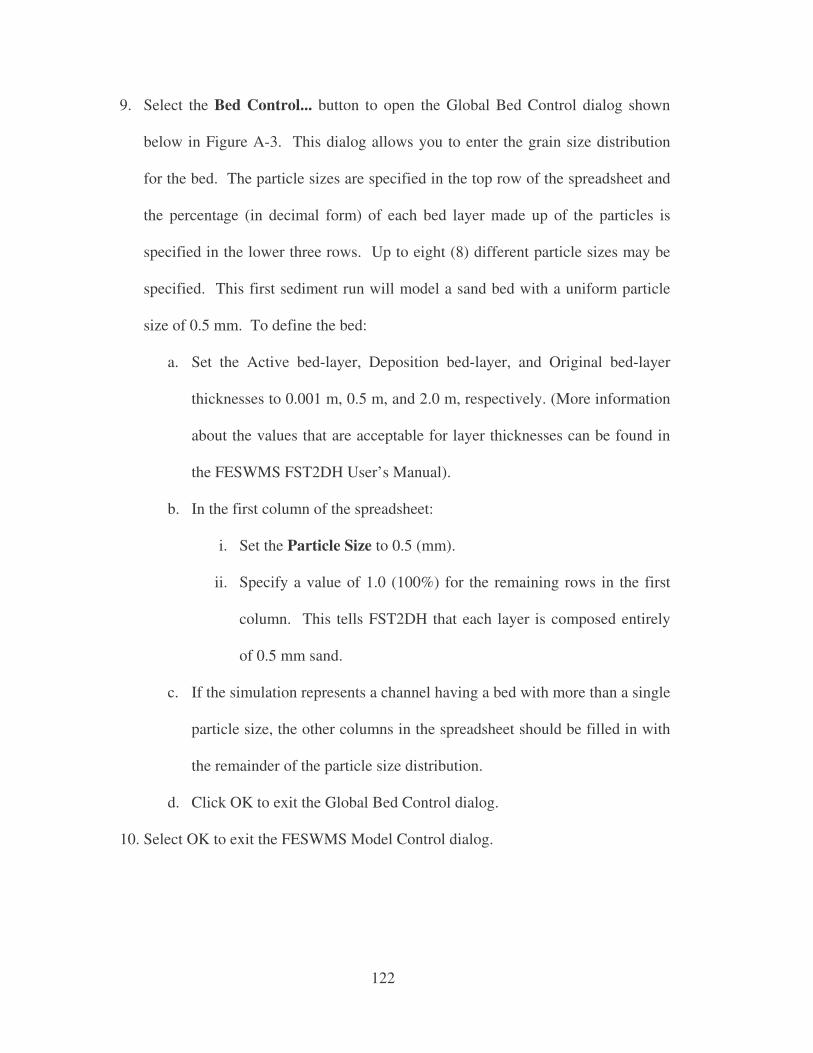
122
9. Select the Bed Control... button to open the Global Bed Control dialog shown
below in Figure A-3. This dialog allows you to enter the grain size distribution
for the bed. The particle sizes are specified in the top row of the spreadsheet and
the percentage (in decimal form) of each bed layer made up of the particles is
specified in the lower three rows. Up to eight (8) different particle sizes may be
specified. This first sediment run will model a sand bed with a uniform particle
size of 0.5 mm. To define the bed:
a. Set the Active bed-layer, Deposition bed-layer, and Original bed-layer
thicknesses to 0.001 m, 0.5 m, and 2.0 m, respectively. (More information
about the values that are acceptable for layer thicknesses can be found in
the FESWMS FST2DH User’s Manual).
b. In the first column of the spreadsheet:
i. Set the Particle Size to 0.5 (mm).
ii. Specify a value of 1.0 (100%) for the remaining rows in the first
column. This tells FST2DH that each layer is composed entirely
of 0.5 mm sand.
c. If the simulation represents a channel having a bed with more than a single
particle size, the other columns in the spreadsheet should be filled in with
the remainder of the particle size distribution.
d. Click OK to exit the Global Bed Control dialog.
10. Select OK to exit the FESWMS Model Control dialog.

123
Figure A-3: FST2DH Global Bed Control Dialog
Specifying Equilibrium Transport Rate Inflow
FST2DH provides the user with several options for the specification of sediment
entering the mesh through the inflow boundary. For this lesson, the equilibrium transport
rate will be applied. For this boundary condition, FST2DH uses flow characteristics to
determine the sediment inflow required to maintain channel equilibrium. To assign this
condition to the inflow boundary:
1. Click the Select Nodestring tool and select the inflow nodestring (at the
lower right corner of the mesh).
2. Select FESWMS | Assign BC…
3. In the Sediment Options Tab, check the toggle for “Specify sediment volumetric
flow rate” and select the “Equilibrium rates applied” radio button (Figure A-4).
4. Click OK to exit the FESWMS Nodestring Boundary Conditions dialog.
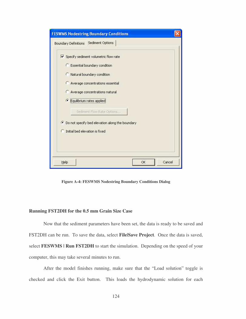
124
Figure A-4: FESWMS Nodestring Boundary Conditions Dialog
Running FST2DH for the 0.5 mm Grain Size Case
Now that the sediment parameters have been set, the data is ready to be saved and
FST2DH can be run. To save the data, select File|Save Project. Once the data is saved,
select FESWMS | Run FST2DH to start the simulation. Depending on the speed of your
computer, this may take several minutes to run.
After the model finishes running, make sure that the “Load solution” toggle is
checked and click the Exit button. This loads the hydrodynamic solution for each

125
timestep. To load the sediment solution, select File|Open and open the file called
“hwy_cross_sed_out.sed” (located in the fst2dh_sediment\output folder). A message will
appear, informing you that the depths given in the solution folder are incorrect. This is
because when the hydrodynamic solution is read in, SMS calculates the depths by
subtracting the initial bed elevation from the water surface elevation computed by
FST2DH instead of the new bed elevations. Click OK to close the message box.
Viewing the Results for the 0.5 mm Grain Size Case
The sediment data file output by FST2DH (*.sed) contains the bed elevations, the
time-derivatives of the bed elevations, the thickness of the active, deposition, and original
bed layers, and additional data specific to each of the particle sizes modeled. To view the
sediment results, select the bed elevation dataset in the project explorer. If the contours
are not on, you may need to turn them on by selecting Display|Contour Options… and
setting the desired contour scheme.
The two main solutions from the model run include the hydrodynamic data
(hwy_cross_sed_out.flo) and the sediment data (hwy_cross_sed_out.sed). Feel free to
explore the datasets contained in these folders in the project explorer. Specifically, you
may want to step through the timesteps to see how the bed elevations change over time.
Creating a Second Sediment Simulation for a Grain Size of 2.0 mm
You will now run a second simulation, with a larger grain size (2.0 mm) for
comparison to the first sediment solution (for 0.5 mm). Before running the simulation

126
with a different grain size, delete the hydrodynamic files (*.flo) from the project explorer
save the project with a new name:
1. Right click on “hwy_cross_out.flo” in the project explorer and select Delete from
the menu that appears.
2. Repeat step 1 for “hwy_cross_sed_out.flo”.
3. Select File | Save As…
4. Change the File name to “hwy_cross_sed_out_2mm.sms” and click Save.
Setting the Sediment Parameters in Model Control
All the options from the previous model were preserved when you saved the
project under a new name. You will now change the particle size that is to be modeled in
the second run:
1. Select FESWMS | Model Control…
2. Select the Sediment Control Tab and then the Bed Control... button to open the
Global Bed Control dialog. Change the particle size from 0.5 mm to 2.0 mm.
3. Exit the dialogs by selecting OK twice.
Running FST2DH for the 2.0 mm Grain Size Case
Save the data (File|Save Project) and run FST2DH (FESWMS | Run FST2DH).
Again, depending on the speed of your computer, this may take several minutes to run.
After the model finishes running, make sure that the “Load solution” toggle is checked
and click the Exit button. The dynamic hydrodynamic solution loads automatically.

127
Select File|Open and open the file called “hwy_cross_sed_out_2mm.sed” (located in the
fst2dh_sediment\output folder). Click OK when the message box appears.
Comparing the Results from the 0.5 mm and 2.0 mm Cases
Feel free to explore the solution for the 2.0 mm simulation. Once you are
through, you can compare the resulting bed elevations from the 0.5 mm and 2.0 mm
simulations. While this can be done in many ways, the following steps outline one
method:
1. Open the data calculator (Data|Data Calculator…)
2. Select “v. bed elevation” from the list of datasets, check the Use all time steps
toggle box, and click Add to Expression.
3. Click the minus “-“ button.
4. Repeat step 2 for the “i. bed elevation” dataset.
5. Change the Result to “diff_bed” and click Compute to create the new dataset.
6. Once the calculation is complete, click Done to exit the Data Calculator.
7. In the project explorer, select the “diff_bed” dataset.
8. Loop through the timesteps to see the difference in bed elevations predicted by
the two simulations. You will notice that the largest differences occur in the areas
of the most scour and deposition—through the contraction and just downstream
from it.
After you have finished any additional analysis you desire to complete, select
File|Exit to exit SMS.

128
Conclusion
In this lesson you have set up and run a steady-state hydrodynamic simulation in
FST2DH and used that hydrodynamic solution as a hotstart file for two separate semi-
coupled sediment simulations for different particle sizes.


