
Applications of nonlinear ODE systems:
Physics: spring-mass system, planet motion, pendulum
Chemistry: mixing problems, chemical reactions
Biology: ecology problem, neural conduction, epidemics
Economy: economic growth, competition
Finance: stochastic equations
1
Population models with interactions:
dx
dt= a(x) + b(x, y)
dy
dt= c(y) + d(x, y)
a(x): self-growth rate of x
b(x, y): effect of interaction on x
c(y): self-growth rate of y
d(x, y): effect of interaction on y
2

predator-prey: a: prey, b: predator
a(x) > 0, b(x, y) < 0, c(y) < 0 and d(x, y) > 0
Example: Canadian lynx and hare, fox and rabbit, ...
competition:
a(x) > 0, b(x, y) < 0, c(y) > 0 and d(x, y) < 0
Example: tiger and lion, rabbit and sheep,
USA and Japan in WWII, ...
cooperative (mutualism):
a(x) < 0, b(x, y) > 0, c(y) < 0 and d(x, y) > 0
Example: plant and pollinator
3
A system of nonlinear differential equations:
dx
dt= 2x(1−
x
2)− xy
dy
dt= 3y(1−
y
3)− 2xy
A competition model, with x and y both grow at a logistic rate,
and the competing for the same food source slows down the
growth of both species
Questions to study: what are the qualitative behavior of the
nonlinear system? Given an initial value, what is the fate of both
species?
4
Studies of phase portrait (1): nullclines
dx
dt= f(x, y)
dy
dt= g(x, y)
The sets f(x, y) = 0 and g(x, y) = 0 are curves on the phase
portrait, and these curves are called nullclines.
The set f(x, y) = 0 is the x-nullcline, where the vector field (f, g)
is vertical.
The set g(x, y) = 0 is the y-nullcline, where the vector field (f, g)
is horizontal.
5
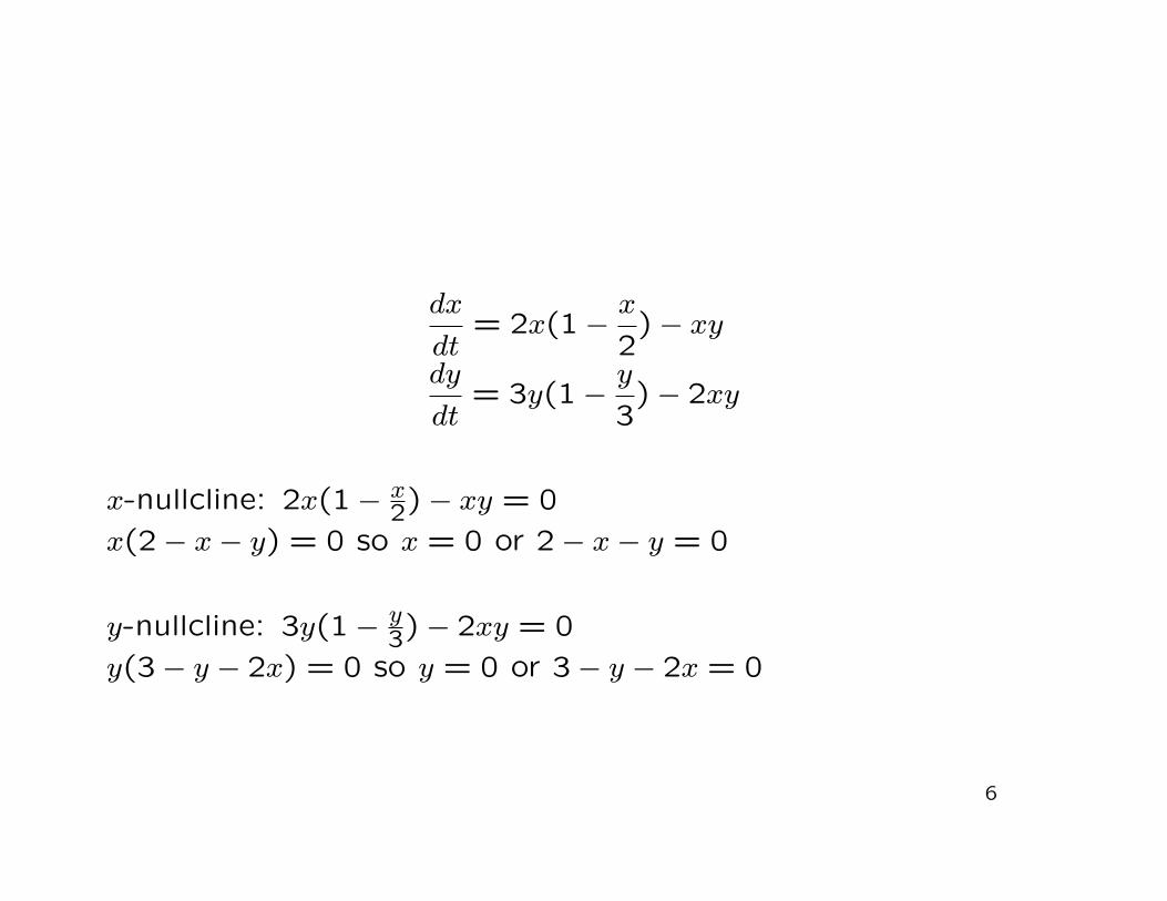
dx
dt= 2x(1−
x
2)− xy
dy
dt= 3y(1−
y
3)− 2xy
x-nullcline: 2x(1− x2)− xy = 0
x(2− x− y) = 0 so x = 0 or 2− x− y = 0
y-nullcline: 3y(1− y3)− 2xy = 0
y(3− y − 2x) = 0 so y = 0 or 3− y − 2x = 0
6
The nullclines divide the phase portraits into regions, and in each
region, the direction of vector field must be one of the following:
north-east, south-east, north-west and south-west
(So nullclines are where the vector field is exactly east, west,
north and south)
In each region, we use an arrow to indicate the direction.
(In 1-d, we use only up-arrow and down-arrow in phase lines.)
7

dx
dt= 2x(1−
x
2)− xy
dy
dt= 3y(1−
y
3)− 2xy
x-nullcline: x = 0 or 2− x− y = 0On x = 0, x′ = 0 and y′ = 3y − y2
On 2− x− y = 0, x′ = 0 and y′ = 3y − y2 − 2y(2− y) = −y + y2
y-nullcline: y = 0 or 3− y − 2x = 0On y = 0, y′ = 0 and x′ = 2x− x2
On 3− y− 2x = 0, y′ = 0 and x′ = 2x− x2− x(3− 2x) = −x + x2
The nullclines divide the region x > 0 and y > 0 to foursub-regions.
8

Studies of phase portrait (2): equilibrium points
dx
dt= f(x, y)
dy
dt= g(x, y)
Equilibrium points are points where f(x, y) = 0 and g(x, y) = 0.
Equilibrium points are the intersection points of x-nullcline and
y-nullcline.
Equilibrium points are constant solutions of the system.
Equilibrium points are also called steady state solutions, fixed
points, etc.
9
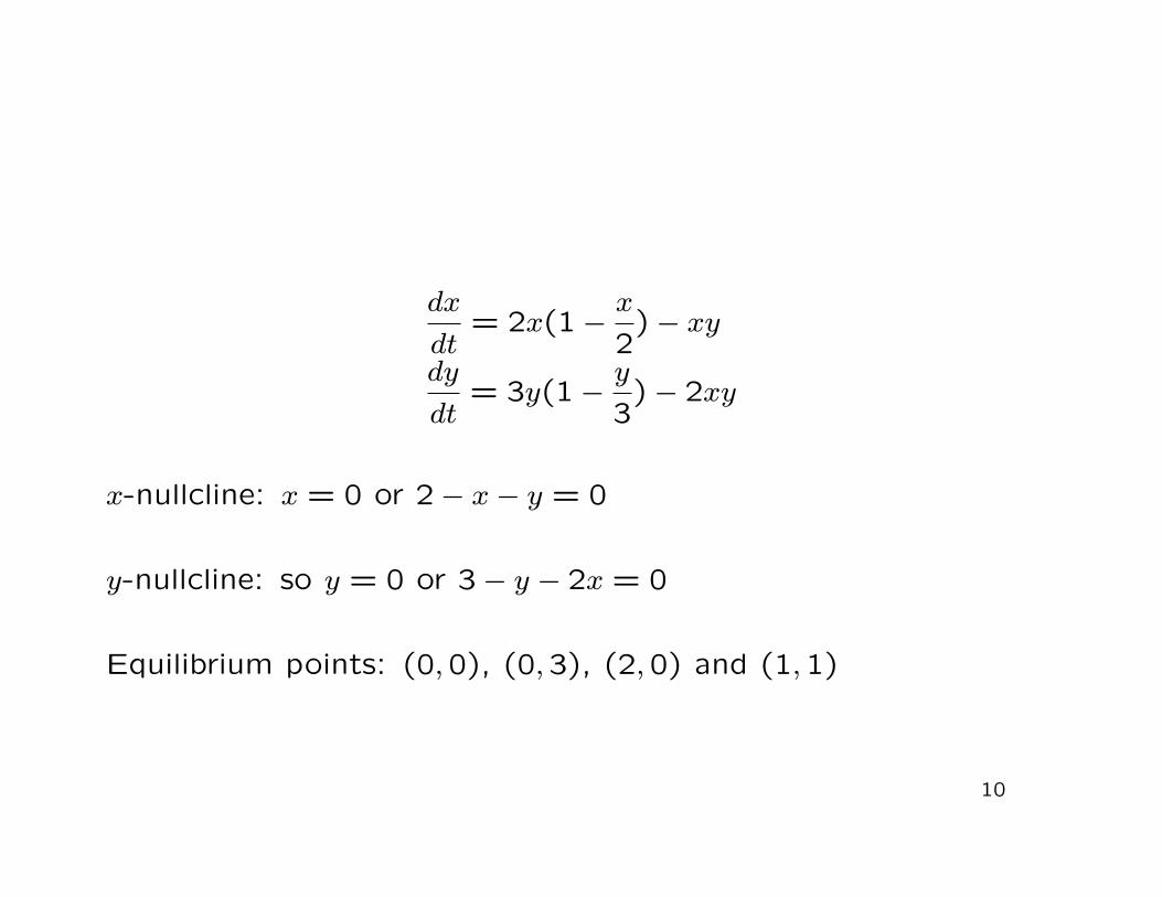
dx
dt= 2x(1−
x
2)− xy
dy
dt= 3y(1−
y
3)− 2xy
x-nullcline: x = 0 or 2− x− y = 0
y-nullcline: so y = 0 or 3− y − 2x = 0
Equilibrium points: (0,0), (0,3), (2,0) and (1,1)
10
Qualitative analysis from nullclines:
Suppose that there is a solution from a point in one of the regions
formed by nullclines, then there is only three possibilities for the
orbit:
A. tends to an equilibrium on the border of this region
B. goes away to infinity
C. enter other neighboring region following the arrow
More information is needed for equilibrium points to further
determination.
11
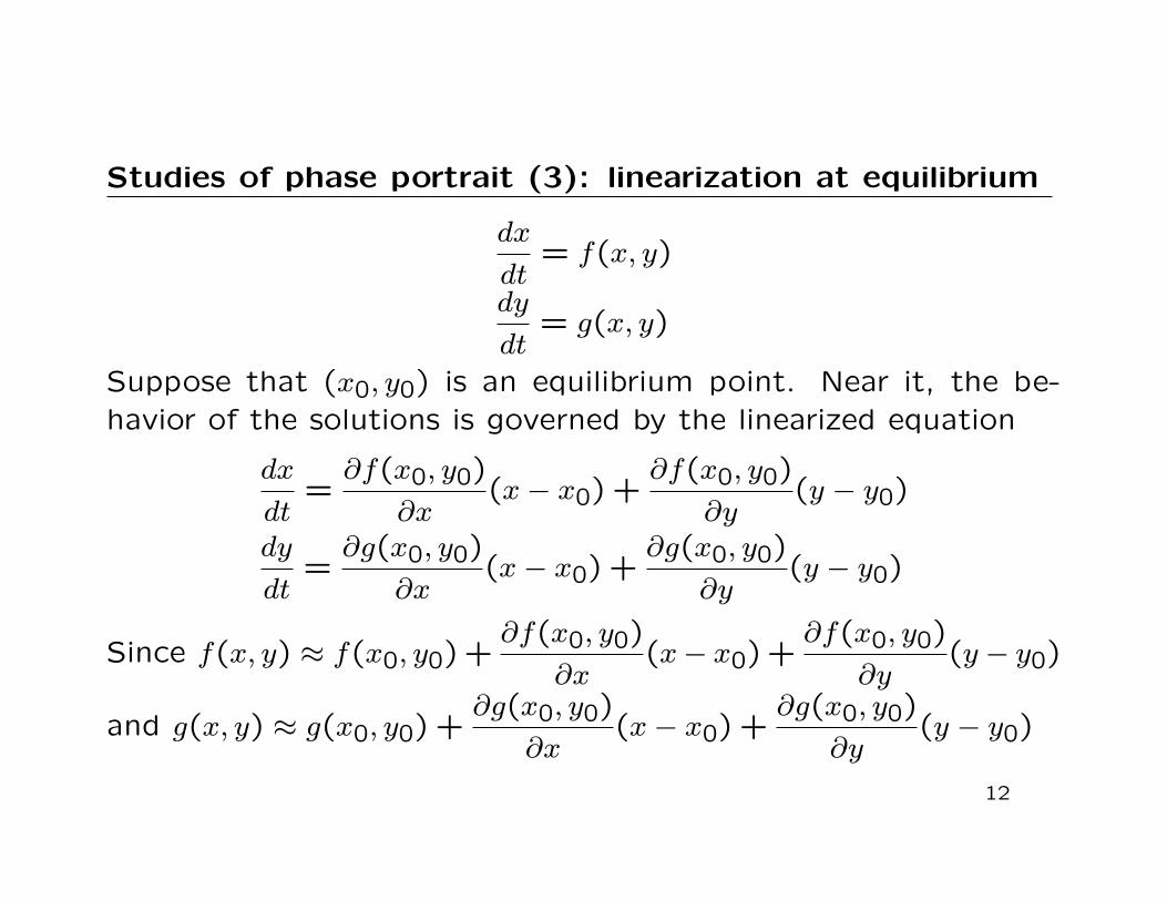
Studies of phase portrait (3): linearization at equilibrium
dx
dt= f(x, y)
dy
dt= g(x, y)
Suppose that (x0, y0) is an equilibrium point. Near it, the be-havior of the solutions is governed by the linearized equation
dx
dt=
∂f(x0, y0)
∂x(x− x0) +
∂f(x0, y0)
∂y(y − y0)
dy
dt=
∂g(x0, y0)
∂x(x− x0) +
∂g(x0, y0)
∂y(y − y0)
Since f(x, y) ≈ f(x0, y0)+∂f(x0, y0)
∂x(x− x0)+
∂f(x0, y0)
∂y(y− y0)
and g(x, y) ≈ g(x0, y0) +∂g(x0, y0)
∂x(x− x0) +
∂g(x0, y0)
∂y(y − y0)
12
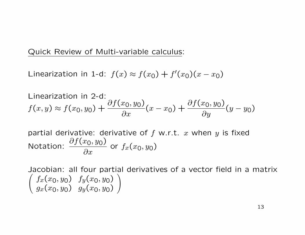
Quick Review of Multi-variable calculus:
Linearization in 1-d: f(x) ≈ f(x0) + f ′(x0)(x− x0)
Linearization in 2-d:
f(x, y) ≈ f(x0, y0) +∂f(x0, y0)
∂x(x− x0) +
∂f(x0, y0)
∂y(y − y0)
partial derivative: derivative of f w.r.t. x when y is fixed
Notation:∂f(x0, y0)
∂xor fx(x0, y0)
Jacobian: all four partial derivatives of a vector field in a matrix(fx(x0, y0) fy(x0, y0)gx(x0, y0) gy(x0, y0)
)
13
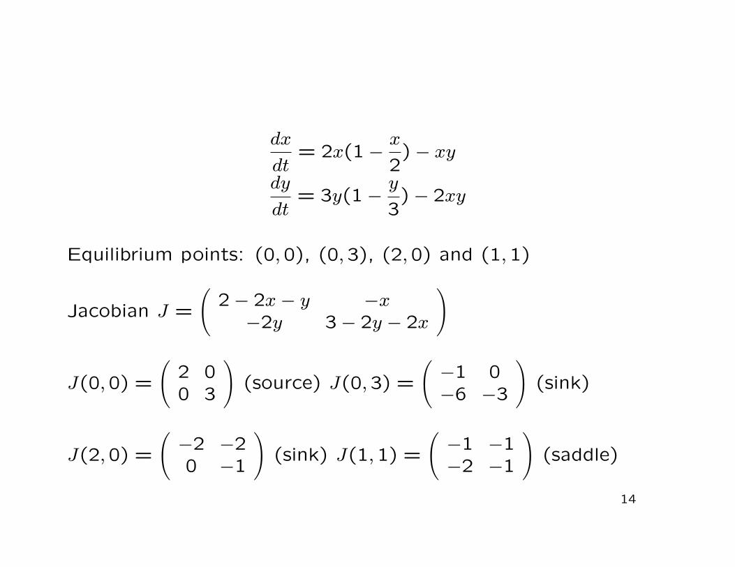
dx
dt= 2x(1−
x
2)− xy
dy
dt= 3y(1−
y
3)− 2xy
Equilibrium points: (0,0), (0,3), (2,0) and (1,1)
Jacobian J =
(2− 2x− y −x−2y 3− 2y − 2x
)
J(0,0) =
(2 00 3
)(source) J(0,3) =
(−1 0−6 −3
)(sink)
J(2,0) =
(−2 −20 −1
)(sink) J(1,1) =
(−1 −1−2 −1
)(saddle)
14
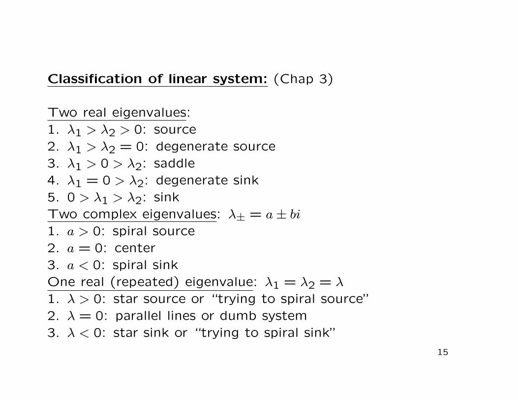
Classification of linear system: (Chap 3)
Two real eigenvalues:1. λ1 > λ2 > 0: source2. λ1 > λ2 = 0: degenerate source3. λ1 > 0 > λ2: saddle4. λ1 = 0 > λ2: degenerate sink5. 0 > λ1 > λ2: sinkTwo complex eigenvalues: λ± = a± bi
1. a > 0: spiral source2. a = 0: center3. a < 0: spiral sinkOne real (repeated) eigenvalue: λ1 = λ2 = λ
1. λ > 0: star source or “trying to spiral source”2. λ = 0: parallel lines or dumb system3. λ < 0: star sink or “trying to spiral sink”
15
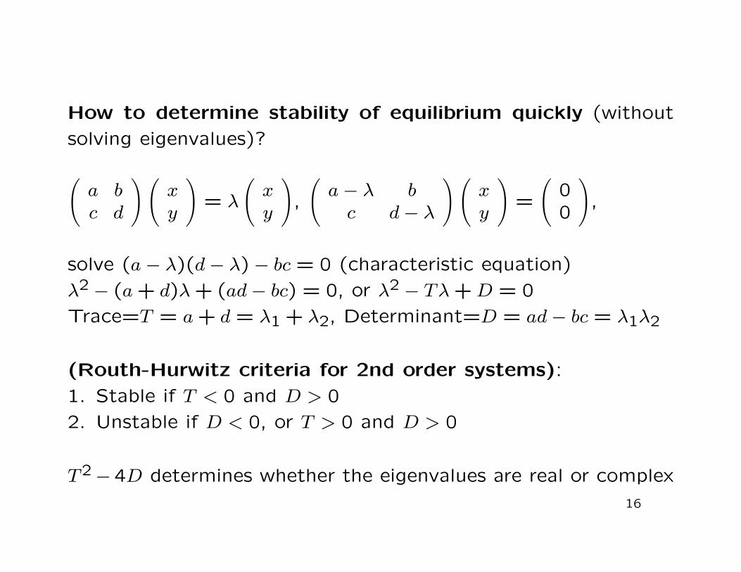
How to determine stability of equilibrium quickly (without
solving eigenvalues)?
(a bc d
)(xy
)= λ
(xy
),
(a− λ b
c d− λ
)(xy
)=
(00
),
solve (a− λ)(d− λ)− bc = 0 (characteristic equation)
λ2 − (a + d)λ + (ad− bc) = 0, or λ2 − Tλ + D = 0
Trace=T = a + d = λ1 + λ2, Determinant=D = ad− bc = λ1λ2
(Routh-Hurwitz criteria for 2nd order systems):
1. Stable if T < 0 and D > 0
2. Unstable if D < 0, or T > 0 and D > 0
T2− 4D determines whether the eigenvalues are real or complex
16

Trace-determinant plane
1. unstable node, source; 2. unstable focus, spiral source;
3. stable focus, spiral sink; 4. stable node, sink; 5. saddle
17
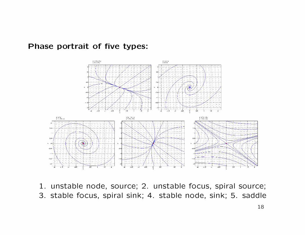
Phase portrait of five types:
1. unstable node, source; 2. unstable focus, spiral source;3. stable focus, spiral sink; 4. stable node, sink; 5. saddle
18
Suppose that P0 = (x0, y0) is an equilibrium point,then a solution Y(t) is a stable orbit of P0 if lim
t→∞Y(t) = P0;
and a solution Y(t) is a unstable orbit of P0 if limt→−∞
Y(t) = P0.
If all solutions nearby are stable orbits, then the equilibrium pointis stable. (sink and spiral sink)If an equilibrium point not stable, then it is unstable. (saddle,source and spiral source)
If the equilibrium point is a saddle point, then there is only onepair of stable orbits, and one pair of unstable orbits. Theseorbits are called separatrices at the saddle point. (separatrixsingular)
When an equilibrium point is stable, the set of all its stable orbitsis called the attraction basin of this equilibrium point.
19

dx
dt= 2x(1−
x
2)− xy
dy
dt= 3y(1−
y
3)− 2xy
At the saddle point (1,1), there is a pair of stable orbits anda pair of unstable orbits, and they are the separatrices of thissaddle point.
Indeed, the stable orbits separates the whole region into twosubregions. In the subregion above this separatrix, all solutionstend to the equilibrium point (0,3) as t →∞; and in the subregionbelow the separatrix, all solutions tend to the equilibrium point(2,0) as t →∞. These two subregions are the attraction basinsof (0,3) and (2,0) respectively.
20
Warning: If the linearized equation at an equilibrium point is adegenerate source, degenerate sink, center, parallel lines, thenthe nonlinear equation may have different phase plane near theequilibrium point.
Linearization Theorem in 2-d: Suppose that (x0, y0) is an equi-librium point of x′ = f(x, y) and y′ = g(x, y), and the eigenvaluesof Jacobian J(x0, y0) are λ1 and λ2.
(1) λ1 > λ2 > 0, then the system is a source;(2) λ1 > 0 > λ2, then the system is a saddle;(3) 0 > λ1 > λ2, then the system is a sink;(4) λ1,2 = a± bi, a > 0, then the system is a spiral source;(5) λ1,2 = a± bi, a < 0, then the system is a spiral sink;(6) If the eigenvalues are other cases, then you need other infor-mation to determine the solution behavior near the equilibriumpoint.
21
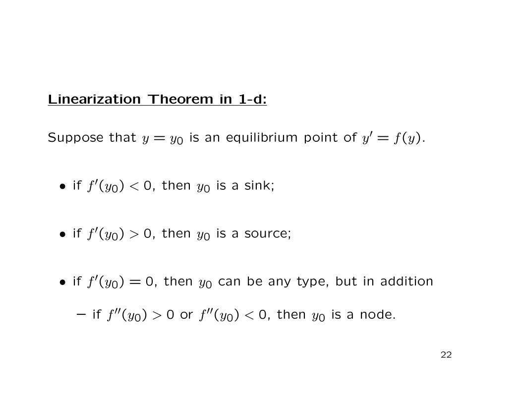
Linearization Theorem in 1-d:
Suppose that y = y0 is an equilibrium point of y′ = f(y).
• if f ′(y0) < 0, then y0 is a sink;
• if f ′(y0) > 0, then y0 is a source;
• if f ′(y0) = 0, then y0 can be any type, but in addition
– if f ′′(y0) > 0 or f ′′(y0) < 0, then y0 is a node.
22
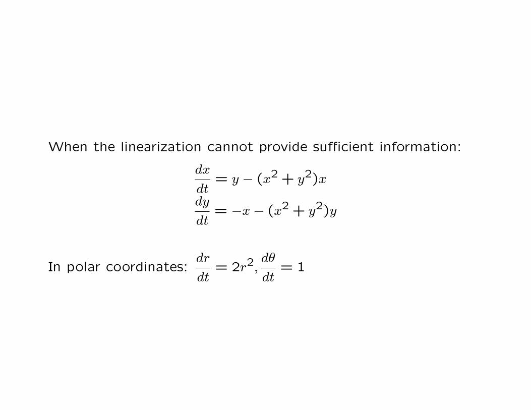
When the linearization cannot provide sufficient information:
dx
dt= y − (x2 + y2)x
dy
dt= −x− (x2 + y2)y
In polar coordinates:dr
dt= 2r2,
dθ
dt= 1
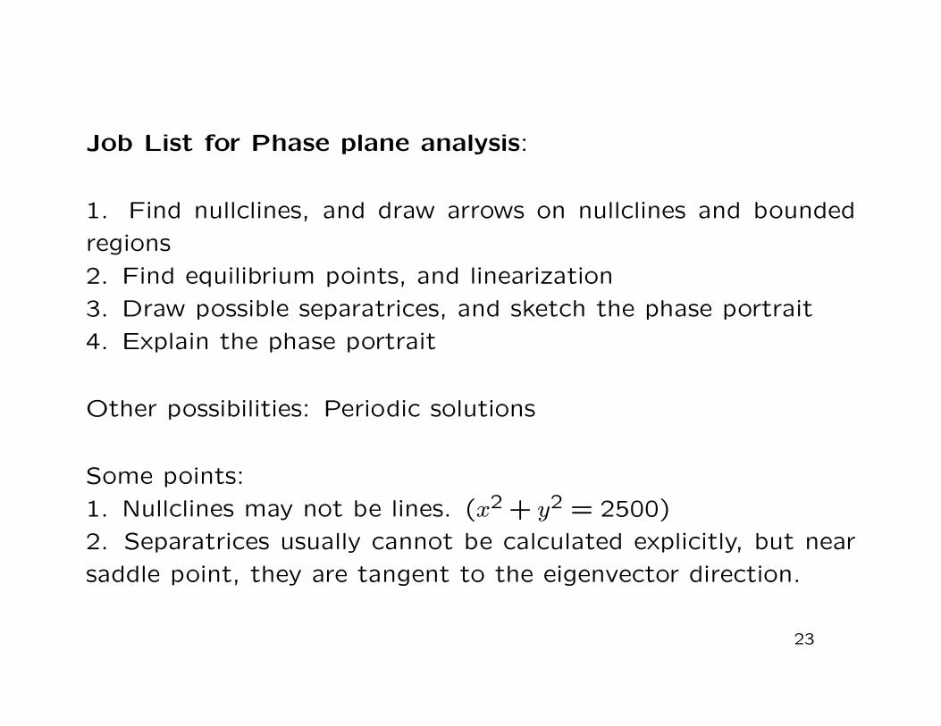
Job List for Phase plane analysis:
1. Find nullclines, and draw arrows on nullclines and bounded
regions
2. Find equilibrium points, and linearization
3. Draw possible separatrices, and sketch the phase portrait
4. Explain the phase portrait
Other possibilities: Periodic solutions
Some points:
1. Nullclines may not be lines. (x2 + y2 = 2500)
2. Separatrices usually cannot be calculated explicitly, but near
saddle point, they are tangent to the eigenvector direction.
23
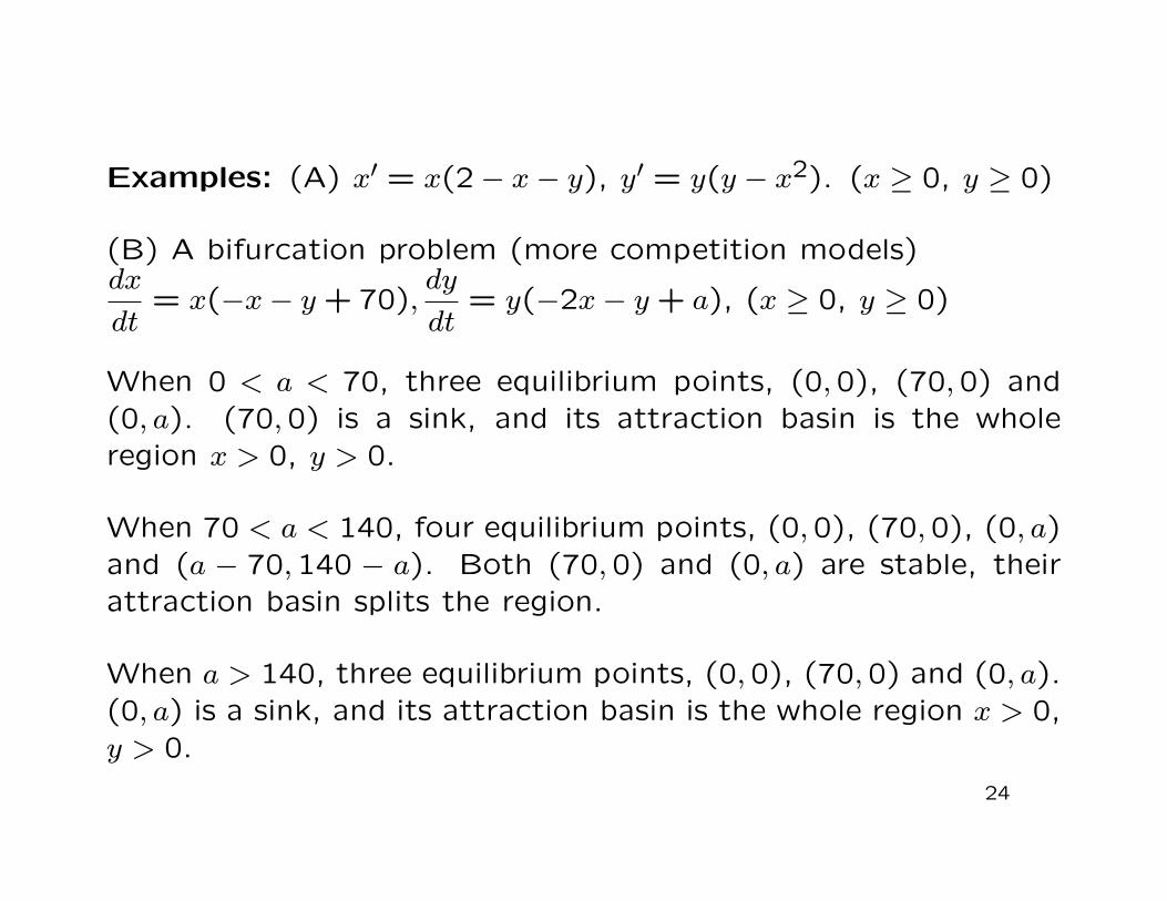
Examples: (A) x′ = x(2− x− y), y′ = y(y − x2). (x ≥ 0, y ≥ 0)
(B) A bifurcation problem (more competition models)dx
dt= x(−x− y + 70),
dy
dt= y(−2x− y + a), (x ≥ 0, y ≥ 0)
When 0 < a < 70, three equilibrium points, (0,0), (70,0) and(0, a). (70,0) is a sink, and its attraction basin is the wholeregion x > 0, y > 0.
When 70 < a < 140, four equilibrium points, (0,0), (70,0), (0, a)and (a − 70,140 − a). Both (70,0) and (0, a) are stable, theirattraction basin splits the region.
When a > 140, three equilibrium points, (0,0), (70,0) and (0, a).(0, a) is a sink, and its attraction basin is the whole region x > 0,y > 0.
24
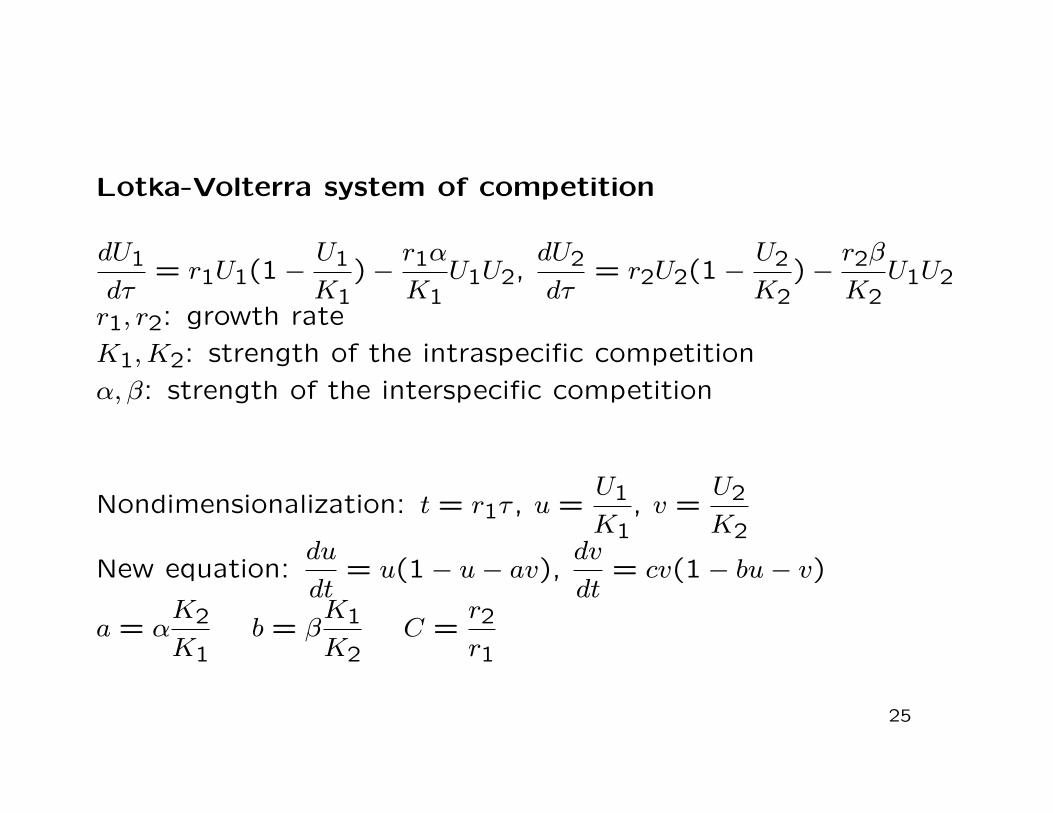
Lotka-Volterra system of competition
dU1
dτ= r1U1(1−
U1
K1)−
r1α
K1U1U2,
dU2
dτ= r2U2(1−
U2
K2)−
r2β
K2U1U2
r1, r2: growth rate
K1, K2: strength of the intraspecific competition
α, β: strength of the interspecific competition
Nondimensionalization: t = r1τ , u =U1
K1, v =
U2
K2
New equation:du
dt= u(1− u− av),
dv
dt= cv(1− bu− v)
a = αK2
K1b = β
K1
K2C =
r2r1
25

Equilibrium points:
(0,0) (extinction), (1,0) (u wins), (0,1) (v wins),
(u∗, v∗) = (1− a
1− ab,1− b
1− ab) (coexistence)
Case 1: a < 1 and b < 1, (u∗, v∗) is stable
Case 2: a > 1 and b > 1, (u∗, v∗) is unstable, and (0,1), (1,0)
are stable (bistable)
Case 3: a < 1 < b, no (u∗, v∗), (1,0) stable, (0,1) unstable (u is
superior competitor)
Case 4: a > 1 > b, no (u∗, v∗), (0,1) stable, (1,0) unstable (v is
superior competitor)
26
Principle of competition exclusion (Gause 1934)
From textbook: if two species occupy the same ecological niche,
then one of them will go extinct.
An ecological niche is mode of existence that a species has within
an ecosystem. Essentially it is the sum of all activities and rela-
tionships a species has while obtaining and using the resources
needed to survive and reproduce.
A species’ niche includes: (a). Habitat - where it lives in the
ecosystem; (b). Relationships - all interactions with other species
in the ecosystem; (c). Nutrition - its method of obtaining food.
27

Another version of Principle of competition exclusion:
If the coexistence (u∗, v∗) satisfiesu∗1
+v∗B≤ 1, then coexistence
is not possible.
Evolution strategy: how to gain competition advantage
r1, r2: growth rate
K1, K2: strength of the intraspecific competition
α, β: strength of the interspecific competition
a = αK2
K1b = β
K1
K2C =
r2r1
K-strategy: increase your carrying-capacity
r-strategy: increase your growth rate
28

Ecological conclusions:
1. Similar species in the same habitat will not coexist.
2. Coexistence will only occur when the competition is less in-
tense (for competition in same niche, ab = αβ = 1)
3. This principle may be not very useful in practice, as we can
always find a way in which two species differ.
4. If two competitors coexist, there is some reason for them to
do so. Or to make two competitors coexist, create difference in
niche.
5. Species may distributed in patchy way, so competition can
be minimized; or time-sharing arrangement with succession of
species or seasonal variability can effect similar result. Gradual
evolution of differing genetic traits (character displacement) to
minimize competition, and more complex multi-species interac-
tions in which predation mediates competition.
29


