ASML alignment sequence generator
Bogdan Mihai Lazăr September 2012

ASML alignment sequence
generator
Bogdan Mihai Lazăr
September 2012

ASML alignment sequence generator
Bogdan Mihai Lazăr
Eindhoven University of Technology
Stan Ackermans Institute / Software Technology
Partners
ASML Eindhoven University of Technology
Steering Group Bogdan Mihai Lazăr
Ed de Gast
Martijn van der Horst
Joost Vromen
István Nagy
Boris Škorić
Date September 2012

Contact
Address
Eindhoven University of Technology
Department of Mathematics and Computer Science
HG 6.57, P.O. Box 513, NL-5600 MB, Eindhoven, The Netherlands
+31402474334
Published by Eindhoven University of Technology
Stan Ackermans Institute
Printed by Eindhoven University of Technology
UniversiteitsDrukkerij
ISBN 978-90-444-1163-8
Abstract ASML is a company that designs, develops and produces photolithography machines, called
wafer scanners, used in the process of manufacturing chips and integrated circuits. In order
to achieve this it requires nanometer accuracy at high speeds. For the nanometer accuracy to
be reached, the system must have a highly accurate calibration system. The calibration is
achieved both through hardware and software means. For the software calibration, the sys-
tem is calibrated through a sequence of measurements which is created manually by an engi-
neer. This report describes the design and implementation of a standalone application that
automatically generates the calibration sequences.
Keywords
ASML, scheme, alignment
Preferred
reference
Bogdan Mihai Lazăr, ASML alignment sequence generator: . Eindhoven University of
Technology, SAI Technical Report, September, 2012.
A catalogue record is available from the Eindhoven University of Technology Library
ISBN: 978-90-444-1163-8 (Eindverslagen Stan Ackermans Instituut ; 2012/061)
Partnership This project was supported by Eindhoven University of Technology and ASML.
Disclaimer
Endorsement
Reference herein to any specific commercial products, process, or service by trade name,
trademark, manufacturer, or otherwise, does not necessarily constitute or imply its endorse-
ment, recommendation, or favoring by the Eindhoven University of Technology or ASML.
The views and opinions of authors expressed herein do not necessarily state or reflect those
of the Eindhoven University of Technology or ASML, and shall not be used for advertising
or product endorsement purposes.
Disclaimer
Liability
While every effort will be made to ensure that the information contained within this report is
accurate and up to date, Eindhoven University of Technology makes no warranty, represen-
tation or undertaking whether expressed or implied, nor does it assume any legal liability,
whether direct or indirect, or responsibility for the accuracy, completeness, or usefulness of
any information.
Trademarks Product and company names mentioned herein may be trademarks and/or service marks of
their respective owners. We use these names without any particular endorsement or with the
intent to infringe the copyright of the respective owners.
Copyright Copyright © 2012. Eindhoven University of Technology. All rights reserved.
No part of the material protected by this copyright notice may be reproduced, modified, or
redistributed in any form or by any means, electronic or mechanical, including photocopy-
ing, recording, or by any information storage or retrieval system, without the prior written
permission of the Eindhoven University of Technology and ASML.

Foreword Computer chips have been getting progressively smaller, faster, and cheaper over the
years. This is made possible by the increase in accuracy and productivity of ASML‘s
lithographic machines. The high-speed, nanometer accuracy in these machines is not
realized by mechatronics alone; software plays an important role as well. Of particu-
lar interest in this project is metrology software that measures and corrects for small
mechanical tolerances. When designing such software a metrologist has to make
trade-offs between accuracy and speed: use accurate, but slow, measurements where
needed and fast, less accurate ones, where possible. The complexity of the machines,
however, makes it hard for a human to oversee the all contingencies of the trade-off,
and come up with a reliable solution that performs as fast as possible. And ASML is
looking for the fastest and most reliable solution, since a machine that reaches the
required accuracy with a higher productivity is very valuable to its customers.
Bogdan‘s goal during this project was to find out if software could help us with this
complex optimization problem. His results show that this is certainly the case. Alt-
hough his work has not reached the point where it can be applied to ASML‘s ma-
chines directly, he has given us many valuable insights into the problem, and provid-
ed us with interesting directions in which the research can be continued. In fact,
ASML is currently in the process of organizing a PhD project on the subject.
It has been a pleasure working with Bogdan on this project. We were especially
amazed by the speed with which he familiarized himself with the domain. It general-
ly takes a new metrologist one to two years to get acquainted with the subject, but
Bogdan only had 9 months. In that time he has not only understood the problem, but
also designed and built an extensible software system for it, experimented with it,
and wrote the thesis you see before you.
In short, Bogdan made a good impression on us. We are glad that he decided to stay,
and that we will be able to continue our cooperation.
Martijn van der Horst
Joost Vromen
27th
of August 2012


iii
Preface This report presents the results of a graduation project for the completion of the
Software Technology programme of the Stan Ackermans Institute of the Tech-
nical University of Eindhoven.
The project was carried out in ASML, a company that designs, develops and pro-
duces photolithography machines. The project made an attempt to prove that the
calibration sequence within an ASML machine can be automatically generated.
The readers that are interested in the global overview of what has been developed
can read the executive summary. The context, domain, problem and stakeholders
information can be found in Chapter 1 to 3. For the readers interested in the re-
quirements, considered approaches and design should read Chapter 4 to 6. The
results, project management and a project retrospective can be found in Chapter 7
to 9. More detailed information about the implementation can be found in Ap-
pendix A and B.
Bogdan Mihai Lazăr
24th
August 2012


v
Acknowledgements
This project could not have been completed without the help of company supervi-
sors. I would like to thank Martijn van der Horst and Joost Vromen for the con-
tinuous support, guidance and feedback throughout the project. Their experienced
insight helped me grasp the technical environment at ASML while their feedback
helped me to continuously develop myself both professionally and technically. I
would also like to thank István Nagy for his experienced insight and active pres-
ence during all the meetings that always took longer than scheduled. I would like
to extend my gratitude to thank Ed de Gast, the group team leader who always
asked the right project questions and steered the project to the right path. I would
like also to thank Roland Bogers and Edwin Boon for their technical inputs.
I am grateful to my university supervisor, Dr. Boris Škorić for assessing my work
and for being an important part of my project steering group. I would like to
thank the program director for PDEng Software Technology, Dr. Ad Aerts, for
his support and management of the entire curriculum of the PDEng program.
Kind words of gratitude to the management assistant, Maggy de Wert for always
being there for all the trainees and for her devotion, enthusiasm and uncondi-
tioned love.
I would like to thank my fellow colleagues for their feedback, support and the
good moments we spent together during and outside the working hours.
Last but not least, I want to thank my parents, my brother and my girlfriend for
their love and support.
Bogdan Mihai Lazăr
24th
August 2012


vii
Executive Summary
ASML is a company that designs, develops and produces photolithography ma-
chines, called wafer scanners, used in the process of manufacturing chips and
integrated circuits. In order to achieve this it requires nanometer accuracy at high
speeds. For the nanometer accuracy to be reached, the system must have a highly
accurate calibration system. The calibration is achieved both through hardware
and software means. For the software calibration, the system is calibrated through
a sequence of measurements which is created manually by an engineer. The pro-
cess is inadequate in the following aspects:
Judging whether a scheme is robust can only be done by an engineer
based on his/hers knowledge and experience. The judgment is error
prone. This leads to unnecessary complex calibration sequences.
The engineer‘s knowledge and experience does not always guarantee
that the created sequence is also the fastest sequence that reaches the
targeted accuracy. This means that the schemes created by the engineer
are not always optimal when the execution time is considered.
It becomes much harder for an engineer to create good sequences as the
complexity of the system increases.
To solve this problem, I designed and implemented a system containing two
components, which are as follows:
The evaluator component which assesses the sequences and gives details
about the execution time, the level of accuracy and the robustness the
sequence provides.
The generator component that creates optimal sequences given the me-
chanical tolerance specifications of the system.
The results of the endeavor are that:
An automated process that creates the sequences was created.
The generated sequences guarantee that the calibration will not fail for
the systems that are compliant to the given mechanical tolerances.
The generated sequence provides the required accuracy level but has the
shortest execution time.
The designed system provides a foundation to carry the further investigation for
an automated sequence generator that will remove the robustness uncertainties
and that will provide an optimal sequence for ASML machines calibration. I rec-
ommend improving the generation time by reducing the resource usage and by
improving the sequence evaluation time.

ix
Table of Contents
Foreword .................................................................................................... i
Preface ...................................................................................................... iii
Acknowledgements ................................................................................... v
Executive Summary ................................................................................ vii
Table of Contents ..................................................................................... ix
List of Figures .......................................................................................... xi
List of Tables .......................................................................................... xiii
1. Introduction ..................................................................................... 15
1.1 Context ....................................................................................... 15
1.2 Outline ........................................................................................ 17
2. Problem Analysis ............................................................................. 19
2.1 Problem overview ....................................................................... 19
2.2 Stakeholders ............................................................................... 19
3. Domain Analysis .............................................................................. 21
3.1 The Wafer to Reticle alignment .................................................. 21
3.2 Domain characteristics .............................................................. 24
4. System Requirements ...................................................................... 27
4.1 Research questions ..................................................................... 27
4.2 Use cases .................................................................................... 28 4.2.1. Evaluate a scheme ................................................................... 28 4.2.2. Generate a scheme ................................................................... 28
4.3 Functional requirements ............................................................ 29
4.4 Non-functional requirements...................................................... 30
4.5 Design competencies .................................................................. 31
5. Approaches....................................................................................... 33
5.1 Introduction ................................................................................ 33
5.2 Standard normal distribution approach ..................................... 33
5.3 Range algebra approach ............................................................ 33
5.4 Worst case scenario approach ................................................... 34
6. System Design .................................................................................. 35
6.1 Introduction ................................................................................ 35
x
6.2 System architecture .................................................................... 36
6.3 Scenarios .................................................................................... 37
6.4 Logical view ............................................................................... 37 6.4.1. Data layer ................................................................................. 37 6.4.2. Business layer .......................................................................... 41 6.4.3. Presentation layer .................................................................... 43
6.5 Process view ............................................................................... 45 6.5.1. Evaluator view ......................................................................... 45 6.5.2. Generator view ........................................................................ 46
6.6 Development view....................................................................... 48
6.7 Deployment view ........................................................................ 49
7. Conclusions ...................................................................................... 51
7.1 Results ........................................................................................ 51
7.2 Answered research questions ..................................................... 52 7.2.1. Feasibility research questions .................................................. 52 7.2.2. Scalability research questions .................................................. 52
7.3 Future work ................................................................................ 56
8. Project Management ....................................................................... 59
8.1 Milestone Trend Analysis ........................................................... 59
8.2 Risks management ...................................................................... 60
9. Project Retrospective ...................................................................... 63
9.1 Good practices ........................................................................... 63
9.2 Design competencies revisited ................................................... 63
Appendix A .............................................................................................. 65
Appendix B .............................................................................................. 73
Glossary ................................................................................................... 81
Bibliography ............................................................................................ 83
About the Authors .................................................................................. 85

xi
List of Figures
Figure 1.1-1: Photolithography workflow ............................................................15 Figure 1.1-2: Perfect overlay ................................................................................16 Figure 1.1-3: Overlay influenced by sensor noise during alignment ....................17 Figure 3.1-1: Measurement and exposure sides ....................................................21 Figure 3.1-2: TIS fiducial .....................................................................................22 Figure 3.1-3: TIS alignment .................................................................................23 Figure 3.1-4: Marks R1 and R2 alignment ...........................................................24 Figure 3.2-1: Readable content of a scheme file ...................................................24 Figure 4.2-1: UML use cases diagram ..................................................................28 Figure 6.1-1: 4+1 views ........................................................................................36 Figure 6.2-1: Overall system architecture .............................................................36 Figure 6.3-1: Evaluate a scheme command ..........................................................37 Figure 6.3-2: Generate a scheme command ..........................................................37 Figure 6.4-1: Parser package class diagram ..........................................................38 Figure 6.4-2: SystemData package class diagram ................................................40 Figure 6.4-3: Evaluator package class diagram ....................................................42 Figure 6.4-4: Generator package class diagram ....................................................44 Figure 6.5-1: Evaluator sequence diagram ...........................................................45 Figure 6.5-2: Evaluator activity diagram ..............................................................46 Figure 6.5-3: Generator sequence diagram ...........................................................47 Figure 6.5-4: Generator activity diagram .............................................................48 Figure 6.6-1: AASG component diagram .............................................................49 Figure 7.1-1: Scheme created by an engineer .......................................................51 Figure 7.1-2: Scheme generated by the application ..............................................51 Figure 7.2-1: Influence of parameters number on the number of schemes
generated ......................................................................................................53 Figure 7.2-2: Influence of the scan types on the number of generated schemes ...54 Figure 7.2-3: Influence of the number of scenarios on a scheme's evaluation time
.....................................................................................................................55 Figure 7.3-1: Remove scenarios ...........................................................................57 Figure 8.1-1: MTA graph .....................................................................................60 Figure 9.2-1: The space of a system defined by a w that has only two parameters
.....................................................................................................................66 Figure 9.2-2: Scheme tree structure ......................................................................76 Figure 9.2-3: Pruning invalid and accurate schemes ............................................78


xiii
List of Tables
Table 1.1-1: ASML's machine subsystems ...........................................................16 Table 2.2-1: Organizational stakeholders .............................................................20 Table 2.2-2: Technical stakeholders .....................................................................20 Table 4.1-1: Feasibility questions .........................................................................27 Table 4.1-2: Scalability questions .........................................................................27 Table 4.2-1: Evaluate a scheme use case ..............................................................28 Table 4.2-2: Generate a scheme use case..............................................................28 Table 4.3-1: Functional requirements ...................................................................29 Table 4.4-1: Quality requirements ........................................................................30 Table 6.4-1: Parser package classes ......................................................................39 Table 6.4-2: SystemData package classes ............................................................39 Table 6.4-3: Evaluator package classes ................................................................41 Table 6.4-4: Generator package classes ................................................................43 Table 7.2-1: Feasibility research questions ...........................................................52 Table 7.2-2: Scalability research questions ..........................................................55 Table 8.2-1: Potential risks ...................................................................................60 Table 9.2-1: Scan action information ...................................................................73 Table 9.2-2: Model action information .................................................................73

15
1.Introduction
This chapter introduces the context in which the ASML alignment sequence genera-
tor (AASG) was created and presents the outline of the paper.
1.1 Context ASML is the world's leading provider of lithography systems for the semiconductor
industry, manufacturing complex machines that are critical to the production of inte-
grated circuits or chips. ASML constantly improves the manufacturing process by
continually shrinking line widths (reduced resolution or feature size), thereby
enabling customers to cut the size or add more functionality to future generations of
ICs. Finer widths allow electricity to move across the chip faster, boosting the chip's
performance [1].
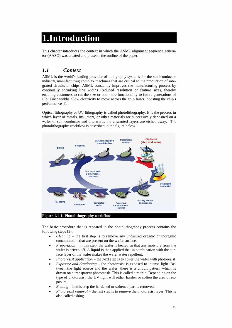
Optical lithography or UV lithography is called photolithography. It is the process in
which layer of metals, insulators, or other materials are successively deposited on a
wafer of semiconductor and afterwards the unwanted layers are etched away. The
photolithography workflow is described in the figure below.
Figure 1.1-1: Photolithography workflow
The basic procedure that is repeated in the photolithography process contains the
following steps [2]:
Cleaning – the first step is to remove any undesired organic or inorganic
contaminators that are present on the wafer surface.
Preparation – in this step, the wafer is heated so that any moisture from the
wafer is driven off. A liquid is then applied that in combination with the sur-
face layer of the wafer makes the wafer water repellent.
Photoresist application – the next step is to cover the wafer with photoresist
Exposure and developing – the photoresist is exposed to intense light. Be-
tween the light source and the wafer, there is a circuit pattern which is
drawn on a transparent photomask. This is called a reticle. Depending on the
type of photoresist, the UV light will either harden or soften the area of ex-
posure.
Etching – in this step the hardened or softened part is removed.
Photoresist removal – the last step is to remove the photoresist layer. This is
also called ashing.
16
Table 1.1-1: ASML's machine subsystems
Subsystem Description
Reticle Handler Delivers reticles to the reticle stage.
Reticle Stage Supports, positions, and moves the reticles accurately
with respect to the lens.
Wafer Handler Delivers wafers to be exposed to the wafer stage and unloads them after exposure.
Wafer Stage Uses a twinstage concept wherein loading, un-loading, measuring and aligning is done in one stage, while exposure is done on the other. The stages work in parallel.
Illumination and Projection Provides the exposure light required to project the reticle image on the wafer.
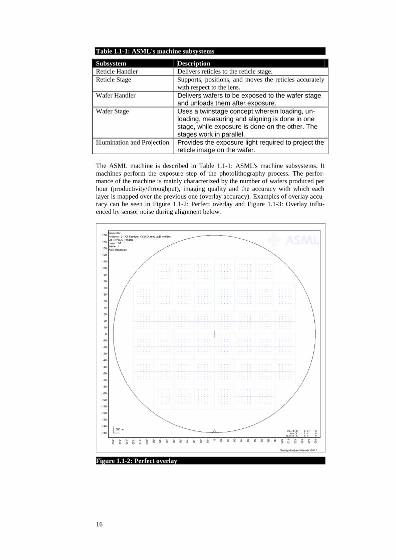
The ASML machine is described in Table 1.1-1: ASML's machine subsystems. It
machines perform the exposure step of the photolithography process. The perfor-
mance of the machine is mainly characterized by the number of wafers produced per
hour (productivity/throughput), imaging quality and the accuracy with which each
layer is mapped over the previous one (overlay accuracy). Examples of overlay accu-
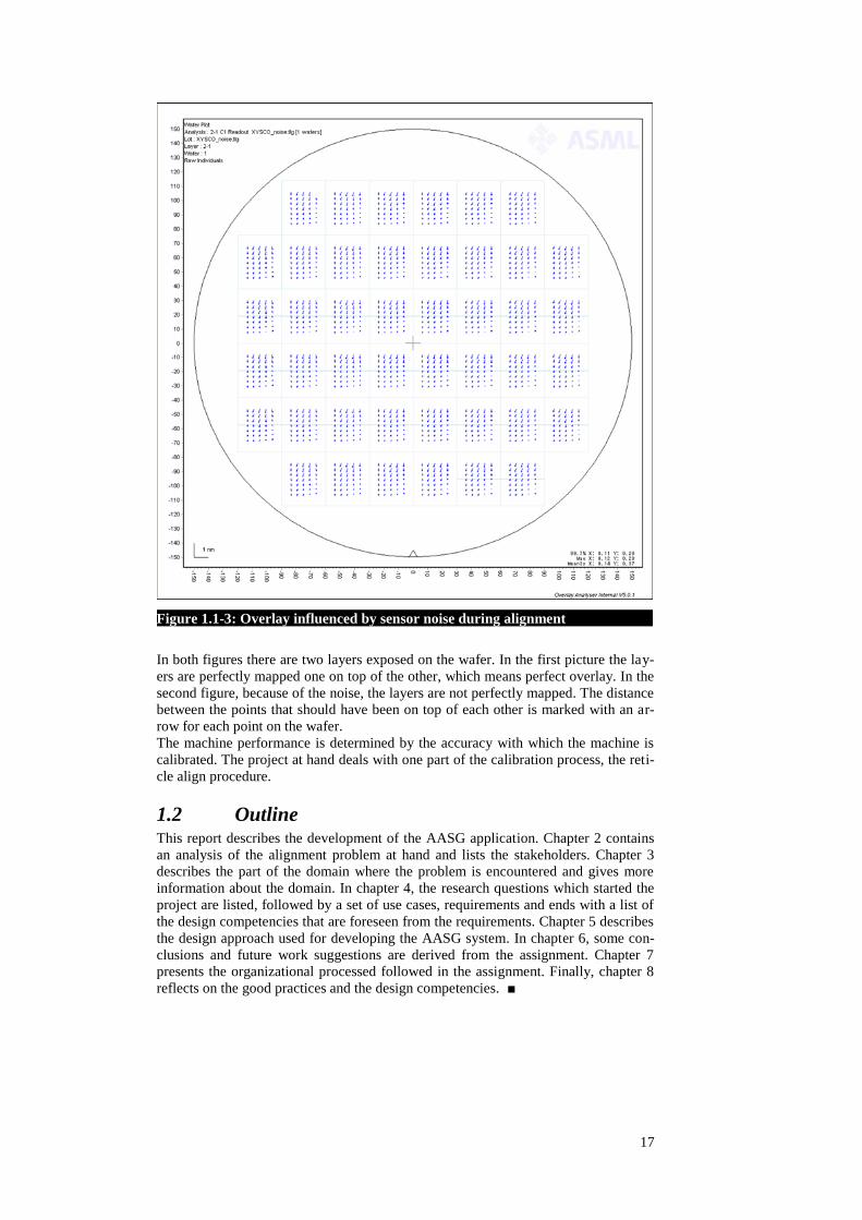
racy can be seen in Figure 1.1-2: Perfect overlay and Figure 1.1-3: Overlay influ-
enced by sensor noise during alignment below.
Figure 1.1-2: Perfect overlay
17
In both figures there are two layers exposed on the wafer. In the first picture the lay-
ers are perfectly mapped one on top of the other, which means perfect overlay. In the
second figure, because of the noise, the layers are not perfectly mapped. The distance
between the points that should have been on top of each other is marked with an ar-
row for each point on the wafer.
The machine performance is determined by the accuracy with which the machine is
calibrated. The project at hand deals with one part of the calibration process, the reti-
cle align procedure.
1.2 Outline This report describes the development of the AASG application. Chapter 2 contains
an analysis of the alignment problem at hand and lists the stakeholders. Chapter 3
describes the part of the domain where the problem is encountered and gives more
information about the domain. In chapter 4, the research questions which started the
project are listed, followed by a set of use cases, requirements and ends with a list of
the design competencies that are foreseen from the requirements. Chapter 5 describes
the design approach used for developing the AASG system. In chapter 6, some con-
clusions and future work suggestions are derived from the assignment. Chapter 7
presents the organizational processed followed in the assignment. Finally, chapter 8
reflects on the good practices and the design competencies. ■
Figure 1.1-3: Overlay influenced by sensor noise during alignment

19
2.Problem Analysis
This chapter presents the problem domain and provides an analysis of the problem at
hand. Section 2.1 introduces the current approach for system calibration. Section 2.2
introduces the stakeholders within the project.
2.1 Problem overview ASML‘s lithography systems described in section 1.1 require nanometer accuracy at
high speeds. For the nanometer accuracy to be reached, the system must have a high-
ly accurate calibration system. To calibrate a system means to measure, compensate
and verify by comparison to a standard. The ASML machines are calibrated through
software. The software calibration is performed on a mathematical model with a se-
quence of measurements and parameter adjustments. The sequence is created by an
engineer who knows the mathematical model that describes the lithography machine
and its imperfections. A sequence should have the following set of properties:
The sequence must be robust: A sequence must be robust for a machine with
inaccuracies within a predefined mechanical tolerance range. This means
that the sequence created can always be performed on any machine that ad-
heres to these mechanical tolerances.
The sequence must be time-optimal: We can demonstrate that there is no
other sequence which can reach the same level of calibration accuracy in
less time.
The sequence must be automatically generated: Having the sequence auto-
matically generated will remove the limitation on computation, knowledge
and experience that of the engineer.
The sequence must be accurate: The sequence must lead the system to an
accuracy which is at least as good as the specified target accuracy.
For an engineer, these properties are hard to achieve because:
Judging whether a sequence is robust can only be done by the engineer
based on his/hers knowledge and experience. The judgment is error prone.
This leads to non-optimal calibration sequences.
The engineer‘s knowledge and experience does not always guarantee that
the created sequence is also the shortest executing sequence that reaches the
targeted accuracy. This means that the sequences created by the engineer are
not always optimal when the execution time is considered.
It becomes much harder for an engineer to create good sequences as the
complexity of the system increases.
2.2 Stakeholders The project identifies two sets of important stakeholders that are directly or indirectly
involved in the project: organizational stakeholders and technical stakeholders.
Organizational stakeholders The organizational stakeholders focus more on the managerial part than on the tech-
nical part. They are more involved in the planning and project management than the
technical aspect.
20
Table 2.2-1: Organizational stakeholders
Name Represents Role
Ad Aerts Program Director of
PDEng in Software
Technology.
Ensure that the final project results meet
the requirements to grant the PDEng in
Software Technology degree.
Boris Škorić University supervisor. Supervisory role in the processes in-
volved during the project.
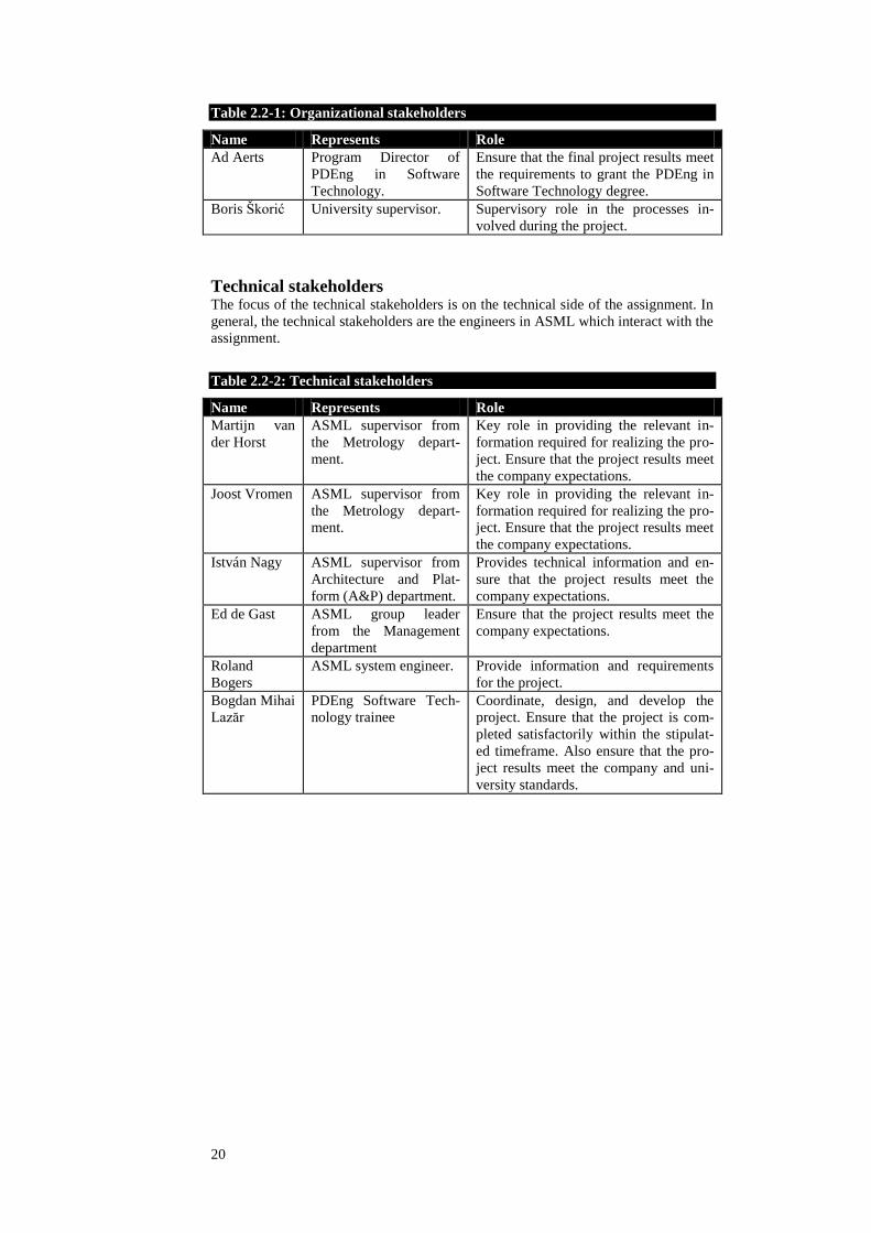
Technical stakeholders The focus of the technical stakeholders is on the technical side of the assignment. In
general, the technical stakeholders are the engineers in ASML which interact with the
assignment.
Table 2.2-2: Technical stakeholders
Name Represents Role
Martijn van
der Horst
ASML supervisor from
the Metrology depart-
ment.
Key role in providing the relevant in-
formation required for realizing the pro-
ject. Ensure that the project results meet
the company expectations.
Joost Vromen ASML supervisor from
the Metrology depart-
ment.
Key role in providing the relevant in-
formation required for realizing the pro-
ject. Ensure that the project results meet
the company expectations.
István Nagy ASML supervisor from
Architecture and Plat-
form (A&P) department.
Provides technical information and en-
sure that the project results meet the
company expectations.
Ed de Gast ASML group leader
from the Management
department
Ensure that the project results meet the
company expectations.
Roland
Bogers
ASML system engineer. Provide information and requirements
for the project.
Bogdan Mihai
Lazăr
PDEng Software Tech-
nology trainee
Coordinate, design, and develop the
project. Ensure that the project is com-
pleted satisfactorily within the stipulat-
ed timeframe. Also ensure that the pro-
ject results meet the company and uni-
versity standards.

21
3.Domain Analysis This chapter presents the domain in which the assignment takes place. It talks about
the components that are encountered during and alignment sequence and about some
characteristics that define the domain.
3.1 The Wafer to Reticle alignment The function of the alignment system is to align the wafer to the reticle. Accurate
alignment is critical because a wafer can be exposed with up to 30 image layers, so
precise and repeated overlay is essential.
There are two locations in the machine where the alignment is performed. These lo-
cations are called sides and there is a measurement side and an exposure side.
In the measurement side the Alignment system measures the position, magnification
and rotation of the wafer with respect to the wafer stage chuck. The chuck is the part
of the wafer stage that carries the wafer and moves it around. The system that does
the alignment on the measurement side is called the Advanced Alignment (AA) sys-
tem. The information obtained on the measurement side will be used on the exposure
side.
On the exposure side the reticle is aligned with respect to the wafer stage chuck. The
system that performs the measurements on the exposure side is called the Transmis-
sion Image Sensor (TIS). Together, the advanced alignment and the transmission
image sensor systems align the reticle to the wafer.
In Figure 3.1-1: Measurement and exposure sides the measurement side is positioned
in the left side and the exposure side on the right.
Figure 3.1-1: Measurement and exposure sides
Each side has a chuck. After the wafer exposure finishes, the chucks are swapped.
Alignment is carried out on the exposure side as well as on the measurement side of
the TWINSCAN. TIS consists of two elements: markers at the reticle level and sen-
sors at the wafer level. The marks are located on the reticle and on the reticle stage
fiducial for alignment. The fiducial is a fixed part of the reticle stage, serving as a
fixed reference point for, among other things, the exchangeable reticle. Extreme UV
or DUV light illuminates these marks. The projection lens captures the diffraction
orders. The diffracted light is then directed down to form an aerial image just below
the projection lens. At a certain position in the aerial image space under the projec-
tion lens, the aerial image is in focus. The transmission image sensor is constructed
22
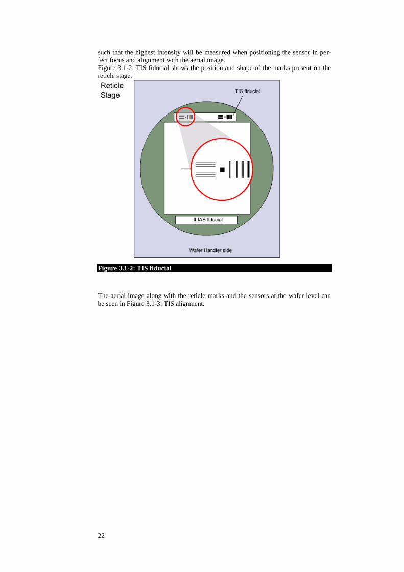
such that the highest intensity will be measured when positioning the sensor in per-
fect focus and alignment with the aerial image.
Figure 3.1-2: TIS fiducial shows the position and shape of the marks present on the
reticle stage.
Figure 3.1-2: TIS fiducial
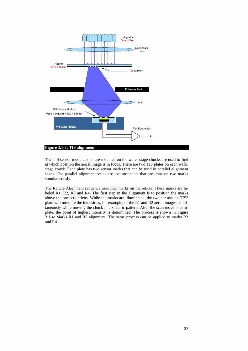
The aerial image along with the reticle marks and the sensors at the wafer level can
be seen in Figure 3.1-3: TIS alignment.
23
Figure 3.1-3: TIS alignment
The TIS sensor modules that are mounted on the wafer stage chucks are used to find
at which position the aerial image is in focus. There are two TIS plates on each wafer
stage chuck. Each plate has two sensor marks that can be used in parallel alignment
scans. The parallel alignment scans are measurements that are done on two marks
simultaneously.
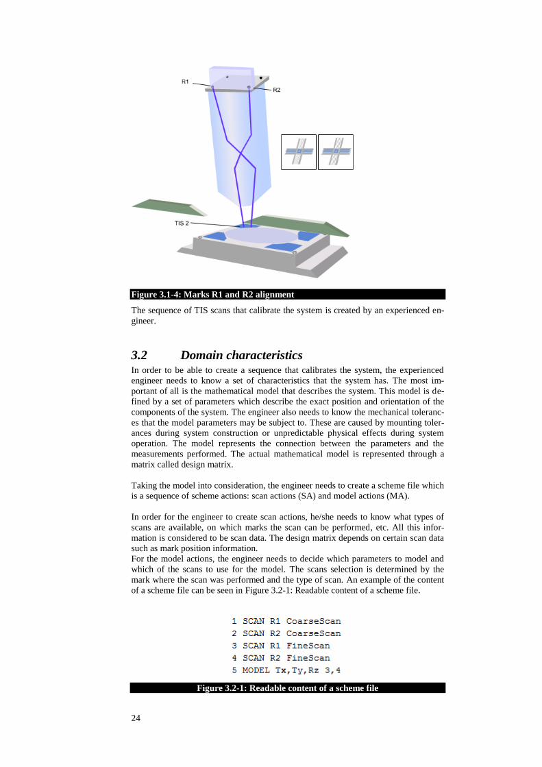
The Reticle Alignment sequence uses four marks on the reticle. These marks are la-
beled R1, R2, R3 and R4. The first step in the alignment is to position the marks
above the projection lens. While the marks are illuminated, the two sensors on TIS2
plate will measure the intensities, for example, of the R1 and R2 aerial images simul-
taneously while moving the chuck in a specific pattern. After the scan move is com-
plete, the point of highest intensity is determined. The process is shown in Figure
3.1-4: Marks R1 and R2 alignment. The same process can be applied to marks R3
and R4.
24
Figure 3.1-4: Marks R1 and R2 alignment
The sequence of TIS scans that calibrate the system is created by an experienced en-
gineer.
3.2 Domain characteristics In order to be able to create a sequence that calibrates the system, the experienced
engineer needs to know a set of characteristics that the system has. The most im-
portant of all is the mathematical model that describes the system. This model is de-
fined by a set of parameters which describe the exact position and orientation of the
components of the system. The engineer also needs to know the mechanical toleranc-
es that the model parameters may be subject to. These are caused by mounting toler-
ances during system construction or unpredictable physical effects during system
operation. The model represents the connection between the parameters and the
measurements performed. The actual mathematical model is represented through a
matrix called design matrix.
Taking the model into consideration, the engineer needs to create a scheme file which
is a sequence of scheme actions: scan actions (SA) and model actions (MA).
In order for the engineer to create scan actions, he/she needs to know what types of
scans are available, on which marks the scan can be performed, etc. All this infor-
mation is considered to be scan data. The design matrix depends on certain scan data
such as mark position information.
For the model actions, the engineer needs to decide which parameters to model and
which of the scans to use for the model. The scans selection is determined by the
mark where the scan was performed and the type of scan. An example of the content
of a scheme file can be seen in Figure 3.2-1: Readable content of a scheme file.
Figure 3.2-1: Readable content of a scheme file

25
Even if all this data is taken into consideration, there is no exact process known to
determine the optimal scheme. ■


27
4.System Requirements
This chapter contains the research questions related to the assignment, a set of system
requirements derived from the research questions which are spread into two catego-
ries: functional and non-functional requirements and a subchapter talks about design
competencies which apply to the assignment.
4.1 Research questions At the start of the project, a set of research questions were created in order to address
the most important issues regarding the assignment. These questions were split up
into two categories: feasibility questions and scalability questions. The research ques-
tions are shown in Table 4.1-1: Feasibility questions and in Table 4.1-2: Scalability
questions below.
Table 4.1-1: Feasibility questions
Feasibility
Question
Is it possible to generate sequences for alignment given the measurement types and
accuracies, mechanical tolerances and the model that relates the two?
Does the duration of the sequence generation fall in an acceptable time frame (few
days)?
Is it possible to have overlay and focus as input parameters for the generator?
Does the generated scheme improve the scheme generated by an expert?
Table 4.1-2: Scalability questions
Scalability
Question
How does the change of accuracy parameters to overlay and focus influence (time)
the scheme generator?
How is the time required by the generator influenced by the number of measurement
types? (Predict scalability based on extension execution time and implementation
time)
How is the time required by the generator influenced by the number of modeled pa-
rameters? (Predict scalability based on extension execution time and implementation
time)
How much time and man hours are needed to add a new measurement type/ model
parameter? (Predict scalability based on extension execution time and implementa-
tion time)
Is there tradeoff between generation time and scheme execution time? If yes, what is
it?
The research questions were used to check the assignment progress and based on the
answer of the questions, continue with the initial planning or take another direction.
Derived from the research questions a set of requirements were created. These re-
quirements were split into functional requirements and non-functional requirements.

28
4.2 Use cases There are only two use cases that describe the assignment: Evaluate a scheme use
case and Generate a scheme use case. These are shown in the figure below. Both of
them can be performed by an Engineer.
Figure 4.2-1: UML use cases diagram
4.2.1. Evaluate a scheme
Table 4.2-1: Evaluate a scheme use case
Primary Actor The Engineer
Context of use The Engineer wants to evaluate a given scheme
Scope AASG system
Precondition The input data describing the system model, scan proper-
ties, mechanical tolerances is correct and available. A
scheme file is already available
Success Guarantees The Engineer receives details about the evaluated scheme:
accuracy and execution time if the scheme is robust or a
fail message if the scheme is not robust
Trigger The Engineer runs the application with a scheme file as a
parameter
Main Success Scenario 1. Engineer: runs the system command with the
available scheme as a parameter.
2. System: evaluates the scheme and produces the
details of the scheme.
4.2.2. Generate a scheme
Table 4.2-2: Generate a scheme use case
Primary Actor The Engineer
Context of use The Engineer wants to generate a scheme
Scope AASG system
Precondition The input data describing the system model, scan proper-
ties, mechanical tolerances is correct and available. A tar-
get accuracy must be set
Success Guarantees The Engineer receives a scheme file that is robust, has the
accuracy lower or equal to the set accuracy and is the fast-
est executing scheme that meets the accuracy specifications
or receives a message that no robust scheme exists that

29
meets the accuracy specifications.
Trigger The Engineer runs the application with no scheme file as a
parameter
Main Success Scenario 1. Engineer: runs the system command with no
scheme as parameter
2. System: generates a scheme file along with its de-
tails.
4.3 Functional requirements In Table 4.3-1: Functional requirements below are shown the most important func-
tional requirements.
Table 4.3-1: Functional requirements
ID Description Priority
FR-1 The system provides details about robustness, accuracy
and execution time of the generated schemes.
Must
FR-2 The system generates measurement and modeling se-
quences based on mechanical tolerances, scan properties
and target accuracy that affect only the horizontal plane.
Must
FR-3 The system accepts accuracy specification in overlay and
focus.
Must
FR-4 The system generates measurement and modeling se-
quences based on mechanical tolerances, scan properties
and target accuracy that affect the horizontal and vertical
plane.
Should
FR-5 The system generates measurements sequences taking
into consideration the possibility of parallel scanning
feature.
Must
FR-6 The system takes into account the non-telecentricity of the
NXE projection optics box.
Should
FR-7 The system generates measurement sequences to support
full reticle align.
Should
FR-8 The system evaluates schemes in order to determine the
accuracy level, the execution time and the robustness of
the scheme.
Could
FR-9 The system gets its mechanical tolerances, scan proper-
ties and target specifications via files.
Must
FR-10 Any sequence generated by the system is guaranteed to
perform all scans within specified capture range for any
system that adheres to the specified mechanical toleranc-
es.
Must
FR-11 The measurement sequence is at least as fast as the one of
the metrology expert, given the condition that both se-
quences have robust measurements.
Must
FR-12 The execution time of the generated measurement se-
quence is as fast as possible given the time constraints of
the generator.
Must
FR-13 The system is within the accuracy specifications. Must
FR-1: The system provides details about accuracy and execution time of the generat-
ed schemes.
In order to identify the optimal solution for a given system description, a set of char-
acteristics need to be specified. These characteristics are scheme accuracy and
scheme execution time. Based on them, the generated schemes can be compared and
thus the optimal scheme can be determined. This requirement refers to the automati-
30
cally generated schemes only. For the engineer created schemes, the evaluation pro-
cess might prove to be more complex and thus FR-8 will cover this case.
FR-2: The system must generate measurement and modeling sequences based on
mechanical tolerances, scan properties and target accuracy that affect only the hori-
zontal plane.
The system is required that for the given input parameters (mechanical tolerances,
scan properties and target accuracy), will generate schemes that model only the pa-
rameters that describe the horizontal plane.
FR-8: The system should be able to evaluate schemes in order to determine the accu-
racy level, the execution time and the robustness of the scheme.
Besides generating schemes, the system can receive a given scheme as input and for
the given scheme it should be able to compute the scheme accuracy, robustness and
execution time. This feature can help compare the scheme generated by the system
with the scheme created by an engineer.
FR-10: Any sequence generated by the system is guaranteed to perform all scans
within specified capture range for any system that adheres to the specified mechani-
cal tolerances.
The requirement guarantees that the generated scheme file will always be robust. By
robust we mean any scheme, generated from specified mechanical tolerances, in
which all the scans are within capture range and in which the model actions can be
performed.
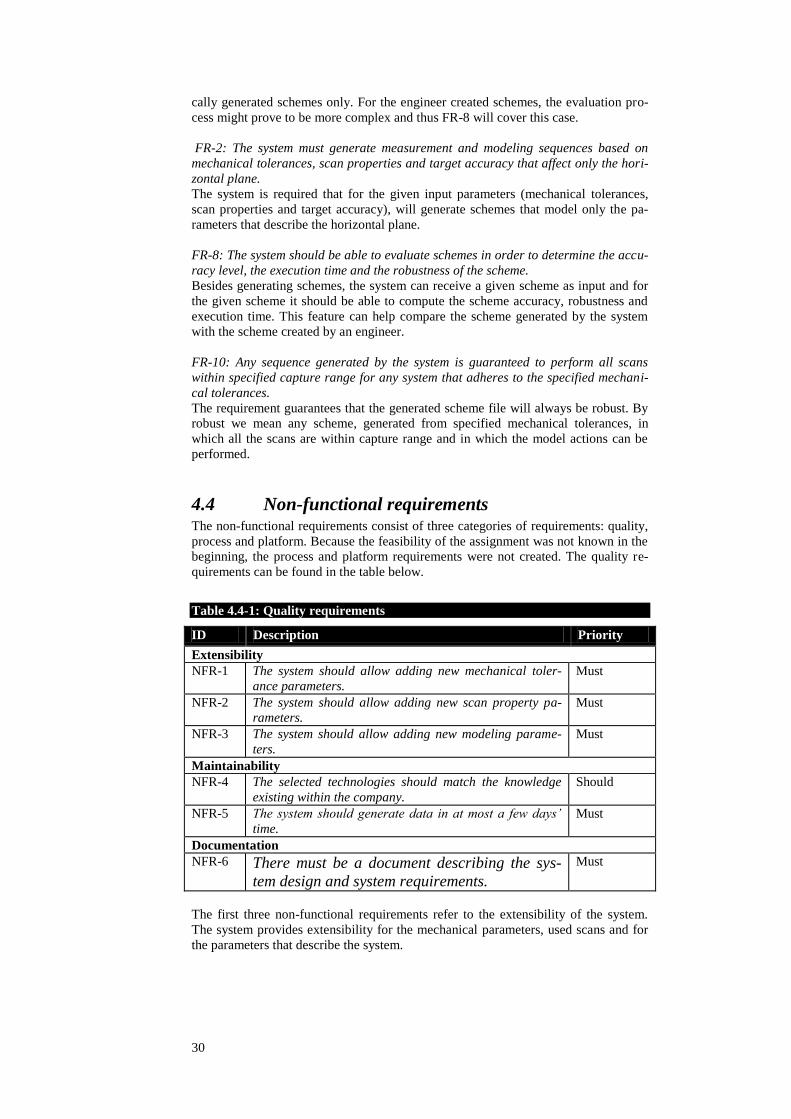
4.4 Non-functional requirements The non-functional requirements consist of three categories of requirements: quality,
process and platform. Because the feasibility of the assignment was not known in the
beginning, the process and platform requirements were not created. The quality re-
quirements can be found in the table below.
Table 4.4-1: Quality requirements
ID Description Priority
Extensibility
NFR-1 The system should allow adding new mechanical toler-
ance parameters.
Must
NFR-2 The system should allow adding new scan property pa-
rameters.
Must
NFR-3 The system should allow adding new modeling parame-
ters.
Must
Maintainability
NFR-4 The selected technologies should match the knowledge
existing within the company.
Should
NFR-5 The system should generate data in at most a few days’
time.
Must
Documentation
NFR-6 There must be a document describing the sys-
tem design and system requirements.
Must
The first three non-functional requirements refer to the extensibility of the system.
The system provides extensibility for the mechanical parameters, used scans and for
the parameters that describe the system.

31
4.5 Design competencies In this section we discuss the design competencies that we foresee based on the re-
quirements. There are five design competencies that are discussed in this chapter:
three relevant and two that are not so relevant to the context of the project. In chapter
9.2 we return to the design competencies to analyze the fulfillment of the design
competencies within the system design.
The three design competencies that are relevant to the context of the project are:
Realizability Some of the research questions were dealing with the possibility of technical realiza-
tion of the assignment. From the beginning of the project there was a concern regard-
ing the complexity of the problem and whether a solution can be created. For this
reason, a prototype on a small model needed to be created as a proof of concept.
Regarding the possibility of economical realization, there was no concern as there is
a wide variety of open source tools that can aid in the development of the tool.
Genericity Because the feasibility of the assignment was not known in the beginning, it was
planned to first create a proof of concept on a small model and afterwards increase it.
For this reason, the initial design needs to have a high level of genericity so that it
can accommodate the future changes.
Functionality
The most important components in the assignment represent the evaluator and gener-
ator which actually create the end product. The evaluator will ease the work of an
engineer to create a new scheme by providing quick feedback on what was created.
The generator component eliminates the human error and provides an optimal solu-
tion.
The two design competencies that are not so relevant to the context of the project are:
Impact Because the current schemes are created manually, the assignment does not influence
the ASML environment in any way. It is a standalone tool.
Elegance Although elegance needs to be considered in any project, it is less important in this
context as a proof of concept will focus more on a working result than on an elegant
one. ■


33
5.Approaches
In this chapter we discuss the alternatives paths the requirements analysis provided
and the reasons behind the chosen alternative.
5.1 Introduction After setting the system requirements, an analysis was needed in order to determine
the solution path that needed to be followed. The reason for the research was because
of the system parameters described in section 3.2 . The value of the system parame-
ters is not known precisely. What is known is the fact that the parameters can take
any value between a minimum value and a maximum value. The range of values
comes from the fact that any machine is built based on a set of system specifications.
These specifications apply to a group of machines even though the parameters that
describe each one of those systems might have different values. Based on this, a
scheme that is generated from a set of parameters that have ranged values instead of
scalars will work for all the systems that the set of parameters describe.
The different representation of the system parameters resulted in several approaches
to be investigated.
5.2 Standard normal distribution approach For the standard normal distribution approach, each parameter can be represented as
a standard normal distribution instead of a range. This means that the middle of the
range would be the mean and the difference between the maximum value and the
mean would have been the standard deviation. The advantages of this approach
would be that if we generate a scheme based on a set of parameters described with
standard normal distribution, we can state the scheme‘s coverage over the systems
described by those parameters. The approach reasons about possible machines in
terms of probabilities and allows us to draw conclusions in the domain of probability
as well. We can say about a scheme that “It is 75% likely to fail”.
The problem with this approach comes when the actual values need to be computed.
As mentioned in section 3.2 , each scheme has scan and model actions. The scans
perform measurements and the model actions update the parameters that describe the
system. In section 3.2 , we introduce the design matrix. Because the parameters that
describe the system can have interdependencies, this means that the design matrix
also depends on the parameters and furthermore will contain elements that are stand-
ard normal distributions. The multiplication and division operations with standard
normal distributions do not result in standard normal distributions [3] [4]. This means
that the updated system parameters will not be known in the same form as before, as
standard normal distributions. The parameter updating procedure is repeated several
times during a calibration sequence so not having the parameters as standard normal
distributions after an update would mean that the approach cannot be done recursive-
ly.
The approach was discarded because of the complexity of the calculations that need
to be performed with the normal distributions.
5.3 Range algebra approach The second approach was to use the parameters as given, as ranges. Because the pa-
rameters were ranges that means that the design matrix that describes the system has
34
elements that have ranges. The reason for this was explained in the previous subsec-
tion.
In order to work with matrices that have elements as ranges, an algebra needed to be
defined. The required operations with matrices are addition, subtraction, multiplica-
tion and inversion. For these operations, the equivalent range algebra properties are
addition, subtraction, multiplication and division.
For the matrices addition, subtraction and multiplication, the properties of the used
ranged algebra are:
• [a, b] + [c, d] = [min (a + c, a + d, b + c, b + d), max (a + c, a + d, b + c, b + d)] =
[a + c, b + d]
• [a, b] − [c, d] = [min (a − c, a − d, b − c, b − d), max (a − c, a − d, b − c, b − d)] =
[a − d, b − c]
• [a, b] × [c, d] = [min (a × c, a × d, b × c, b × d), max (a × c, a × d, b × c, b × d)]
Unfortunately, the division property of the range algebra does not fulfill the require-
ments, as a*b = c does not necessarily means that c/b = a. This is shown in the exam-
ple below.
[-3,5]*[-2,1] = [-10,6]
[-10,6]/[-2,1] = [-10,6]
[-10,6]/[-3,5] = [-2,3.33]
Using the algebra as described will lead to a pessimistic result. More than that, there
is no guarantee that the design matrix with ranged elements can be inverted.
Because there is no algebra for ranges that can meet the requirements thus the ap-
proach was not pursued further on.
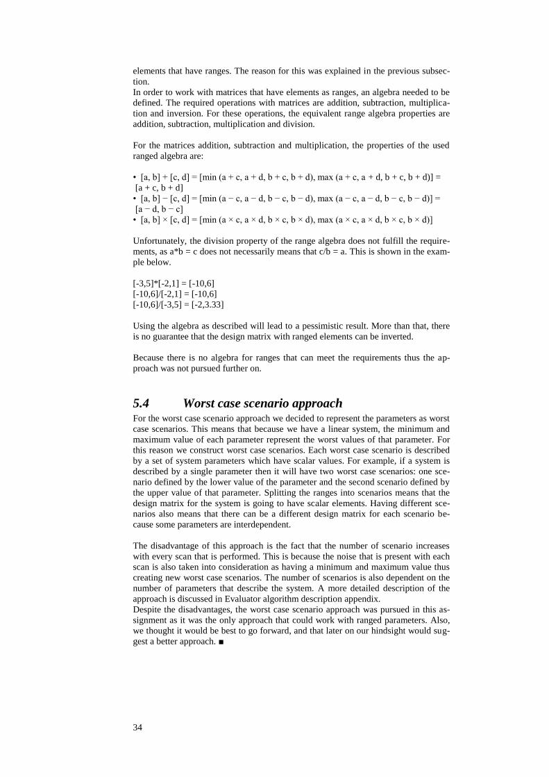
5.4 Worst case scenario approach For the worst case scenario approach we decided to represent the parameters as worst
case scenarios. This means that because we have a linear system, the minimum and
maximum value of each parameter represent the worst values of that parameter. For
this reason we construct worst case scenarios. Each worst case scenario is described
by a set of system parameters which have scalar values. For example, if a system is
described by a single parameter then it will have two worst case scenarios: one sce-
nario defined by the lower value of the parameter and the second scenario defined by
the upper value of that parameter. Splitting the ranges into scenarios means that the
design matrix for the system is going to have scalar elements. Having different sce-
narios also means that there can be a different design matrix for each scenario be-
cause some parameters are interdependent.
The disadvantage of this approach is the fact that the number of scenario increases
with every scan that is performed. This is because the noise that is present with each
scan is also taken into consideration as having a minimum and maximum value thus
creating new worst case scenarios. The number of scenarios is also dependent on the
number of parameters that describe the system. A more detailed description of the
approach is discussed in Evaluator algorithm description appendix.
Despite the disadvantages, the worst case scenario approach was pursued in this as-
signment as it was the only approach that could work with ranged parameters. Also,
we thought it would be best to go forward, and that later on our hindsight would sug-
gest a better approach. ■

35
6.System Design
In this chapter, the system design of the AASG application is presented. Section 6.1
introduces the approach used to describe the system. The architecture of the system is
described in Section 6.2 . The chapter concludes with Sections 6.3 through 6.7
describing the 4+1 views of the system design.
6.1 Introduction Application architecture seeks to build a bridge between business requirements and
technical requirements by understanding use cases and then finding ways of imple-
menting those use cases into software. The goal of the architecture is to identify the
system requirements that affect the structure of the architecture [5]. The ―4+1‖ archi-
tectural view model expresses these requirements in separate views, each describing
the system from the viewpoint of different stakeholders, such as end-users, develop-
ers and project managers [6]. There are five views that help describe the system ar-
chitecture:
Logical view – primarily supports the functional requirements—what the
system should provide in terms of services to its users. The logical architec-
ture is represented by means of class diagrams and class templates [7].
Development view – also known as the implementation view, focuses on
the actual software module organization on the software development envi-
ronment. The development architecture of the system is represented by
module and subsystem diagrams, showing the ‗export‘ and ‗import‘ rela-
tionships [6]. The view uses UML component or package diagrams to de-
scribe the system components.
Process view – addresses issues of concurrency and distribution, of sys-
tem‘s integrity, of fault-tolerance, and how the main abstractions from the
logical view fit within the process architecture—on which thread of control
is an operation for an object actually executed. The UML notations used for
the process view include activity diagrams.
Physical view – also known as deployment view, take into account primari-
ly the non-functional requirements of the system such as availability, relia-
bility (fault-tolerance), performance (throughput), and scalability. The view
depicts the system from a system engineer's point-of-view. It is concerned
with the topology of software components on the physical layer, as well as
the physical connections between these components. UML Diagrams used
to represent physical view include the Deployment diagram.
Scenarios – are in some sense an abstraction of the most important require-
ments. The scenarios describe sequences of interactions between objects,
and between processes. They are used to identify architectural elements and
to illustrate and validate the architecture design.
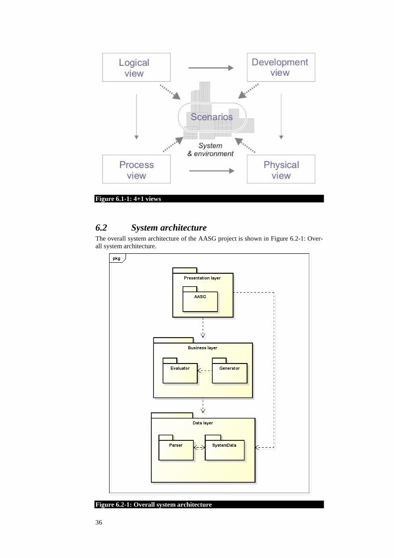
Figure 6.1-1: 4+1 views shows how the views are connected to each other.
36
Figure 6.1-1: 4+1 views
6.2 System architecture The overall system architecture of the AASG project is shown in Figure 6.2-1: Over-
all system architecture.
Figure 6.2-1: Overall system architecture

37
The architecture of a software system generally combines two or more architectural
styles. For this architecture, two architectural styles were used: the layered architec-
tural style and the domain driven design architectural style.
The layered architectural style focuses on the grouping of related functionality within
an application into distinct layers that are stacked vertically on top of each other.
Functionality within each layer is related by a common role or responsibility. Com-
munication between layers is explicit and loosely coupled. Layering your application
appropriately helps to support a strong separation of concerns that, in turn, supports
flexibility and maintainability [5].
The three layers that can be identified are the presentation layer, the business layer
and the data layer
Although, the application does not have a graphical user interface, we consider in this
architecture that the main class, contained in the AASG package, that receives the
input from the command line to act as a presentation layer. The business layer
contains the logic of the application, which consists of the generator and the
evaluator packages. The last layer, the data layer, contains the information that the
system requires to operate and the methods used to get the information from the input
files. The information is stored in objects that describe the domain for which the
application is used. The domain driven design architectural style can only be found in
the data layer.
6.3 Scenarios The scenarios view shows how the users interact with the system. For the AASG
system, there are only two use case scenarios: evaluate a scheme scenario and gener-
ate a scheme scenario. The use cases are described in subchapters 4.2.1. and 4.2.2. .
The Evaluate a scheme use case offers the user the possibility to evaluate a scheme
that was created by an engineer in order to determine its characteristics like robust-
ness, accuracy and execution time. It requires a scheme file to be given as input in the
command parameters.
Figure 6.3-1: Evaluate a scheme command
The Generate a scheme use case will generate a set of schemes which are bound by
the input information. It will then find the fastest execution scheme that meets the
accuracy requirements and which is robust. Such a scheme must exist otherwise the
generator will not return anything. For this use case, the target accuracy parameter
must be included in the command.
Figure 6.3-2: Generate a scheme command
The use cases can be ran with one command that has both the scheme and target ac-
curacy parameters. The evaluation of the scheme is performed first and afterwards, a
new scheme is generated.
6.4 Logical view In this subsection, the logical view of each layer in the system architecture will be
presented. The three layers are data layer, business layer and presentation layer.
6.4.1. Data layer
The data layer is composed of two packages, the Parser package and the SystemData
package. Both packages handle the input information. The Parser package reads the
information from the input files and creates the appropriate data structures in the Sys-

38
temData package. The SystemData package holds the domain data required by the
business layer.
Parser package The Parser package retrieves the information from the input files. A class diagram is
shown in Figure 6.4-1: Parser package class diagram below.
Figure 6.4-1: Parser package class diagram

39
The access point of the package is the Parser class. It receives the name of the input
files that it needs to parse in order to extract the useful information. Each input file
has its own parser class that reads the file and stores the information in a specific
class from the SystemData package. The classes are shown in the table below.
Table 6.4-1: Parser package classes
Class Description
Parser Maintains the parsers
Operation Description
parse Calls the specific parsers
getInputList Returns the list of parsers
ParserStrategy This is the interface for all the parser types
Operation Description
parse Interface function to parse an input
file in order to retrieve the infor-
mation inside it
ConstantParser Implements the constant parser
DesignMatrixParser Implements the design matrix parser
MarksParser Implements the marks parser
MechInaccParser Implements the mechanical tolerances parser
ScansParser Implements the scans parser
SchemeParser Implements the scheme parser
RealMachineParameterParser Implements the real machine parameters parser
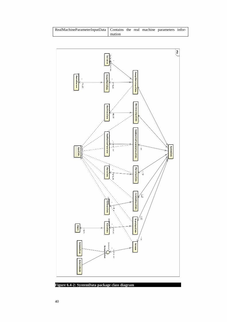
SystemData package
The SystamData package uses the Parser package to transfer the information from the
input files to its own classes. All the data that is required by the Business layer is
found in the SystemData package. The classes in this package are representative to
the domain where the application is used. Figure 6.4-2: SystemData package class
diagram depicts the classes in the SystemData package. The atributes and operations
in Figure 6.4-2: SystemData package class diagram were left out so that the figure is
more readable. The most important classes are described in the table below.
Table 6.4-2: SystemData package classes
Class Description
SystemData The main access point to the domain data in the
SystemData package through the use of getters
and setters.
ConstantInputData Contains the list of constants used in the system.
Provides a connection to the parser to add new
constants and a connection to the business layer
to retrieve the list of constants.
DesignMatrixInputData Contains the model of the system in a matrix
form. It allows new data from the parser to be
added and provides the information to the busi-
ness layer.
MarksInputData Contains the marks information.
MechInaccInputData Contains the information of the mechanical tol-
erances
ScansInputData Contains the scans information
Scheme Contains the information from a scheme
40
RealMachineParameterInputData Contains the real machine parameters infor-
mation
Figure 6.4-2: SystemData package class diagram

41
Strategy pattern
Behavioral patterns are the design patterns that are most specifically concerned with
communication between objects. The strategy patterns is used to encapsulate an
algorithm inside a class. It has been used in both the Parser package and SystemData
package. It imposes the open-closed principle which states that software entities must
be open for extension, but closed for modification.
Using the Strategy pattern will make the application more extendable with low
change impact. For example, if a new set of data needs to be parsed, a new class that
implements the ParserStrategy class can be added. The new class will parse the
required information and add it to a new class in the SystemData package.
6.4.2. Business layer
The business layer consists of two packages: the Evaluator package and the Genera-
tor package. They represent the logic of the application.
The Evaluator package assesses a scheme and retrieves information about its accura-
cy, robustness and execution time. The Generator package, creates schemes, sends
them for evaluation to the Evaluator package and then determines the optimal
scheme. The optimal scheme is determined based on the scheme properties and the
given requirements.
The business layer comunicates only with the Data layer in order to retrieve the
information that is needed to evaluate or generate a scheme.
Evaluator package
The evaluator package retrieves the scheme information from the Data layer. It then
evaluates the scheme based on the actions that the scheme contains. The scheme
contains two types of actions, scan actions and model actions. Figure 6.4-3: Evalua-
tor package class diagram shows the classes contained by the Evaluator package. The
table below presents the classes in more detail.
Table 6.4-3: Evaluator package classes
Class Description
Evaluator Performs the evaluation of a scheme
Operation Description
evaluateScheme Evaluates the scheme that is
saved in the SystemData package.
ModelingActionAnalyzer Evaluates modeling actions
ScanActionAnalyzer Evaluates scan actions
Scenario Describes a scenario based on a set of real machine
parameters and software parameters.

42
Figure 6.4-3: Evaluator package class diagram

43
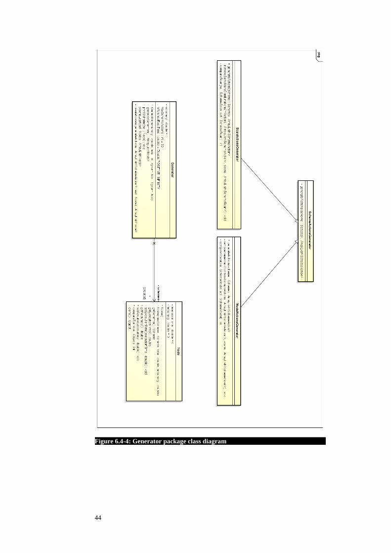
Generator package
The Generator package has the responsibility of generating new schemes based on
the input information. It must find the optimal scheme that meets the given require-
ments by evaluating the most significant schemes from the newly generated ones. It
communicates to the SystemData package in order to retrieve the domain data and
also needs to call the Evaluator in order to evaluate the generated schemes. Figure
6.4-4: Generator package class diagram describes the structure of the Generator
package.
Because a scheme has two different actions, scan action and model actions, each ac-
tion needs a specific generator. Details about the classes are found in Table 6.4-4:
Generator package classes below.
Table 6.4-4: Generator package classes
Class Description
Generator Generates new schemes and finds the optimal one
based on the accuracy, robustness and execution
time requirements.
Operation Description
geenrateSchemes Generates and finds the optimal
scheme.
SchemeActionsGenerator Abstract class for the different types of actions.
Operation Description
geenrateActions Abstract function for scheme
actions generation.
ScanActionsGenerator Implementation for scan actions
ModelActionsGenerator Implementation for the model actions
Node Stores the accuracy, robustness and execution time
details of a scheme.
6.4.3. Presentation layer
The presentation layer consists of the AASG package. The package only contains the
main class. Its main functionality is to parse the command arguments, check them
and then initiate the data and business layer classes. The AASG package is consid-
ered to represent the presentation layer because it is the only one that interacts with
the user through the command arguments.
44
Figure 6.4-4: Generator package class diagram
45
6.5 Process view The process view addresses issues of concurrency and distribution, of system‘s integ-
rity, of fault-tolerance, and how the main abstractions from the logical view fit within
the process architecture. The view presents the communication between the classes
related to the two use cases presented in subchapters 4.2.1. and 4.2.2. .
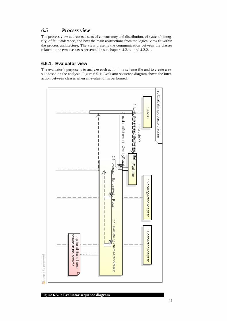
6.5.1. Evaluator view
The evaluator‘s purpose is to analyze each action in a scheme file and to create a re-
sult based on the analysis. Figure 6.5-1: Evaluator sequence diagram shows the inter-
action between classes when an evaluation is performed.
Figure 6.5-1: Evaluator sequence diagram
46
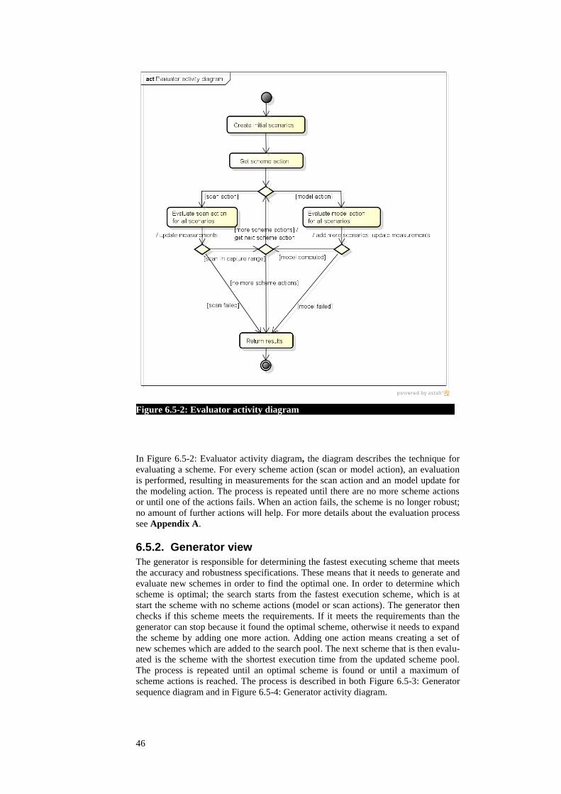
In Figure 6.5-2: Evaluator activity diagram, the diagram describes the technique for
evaluating a scheme. For every scheme action (scan or model action), an evaluation
is performed, resulting in measurements for the scan action and an model update for
the modeling action. The process is repeated until there are no more scheme actions
or until one of the actions fails. When an action fails, the scheme is no longer robust;
no amount of further actions will help. For more details about the evaluation process
see Appendix A.
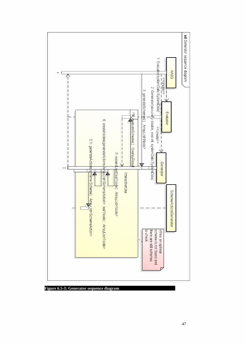
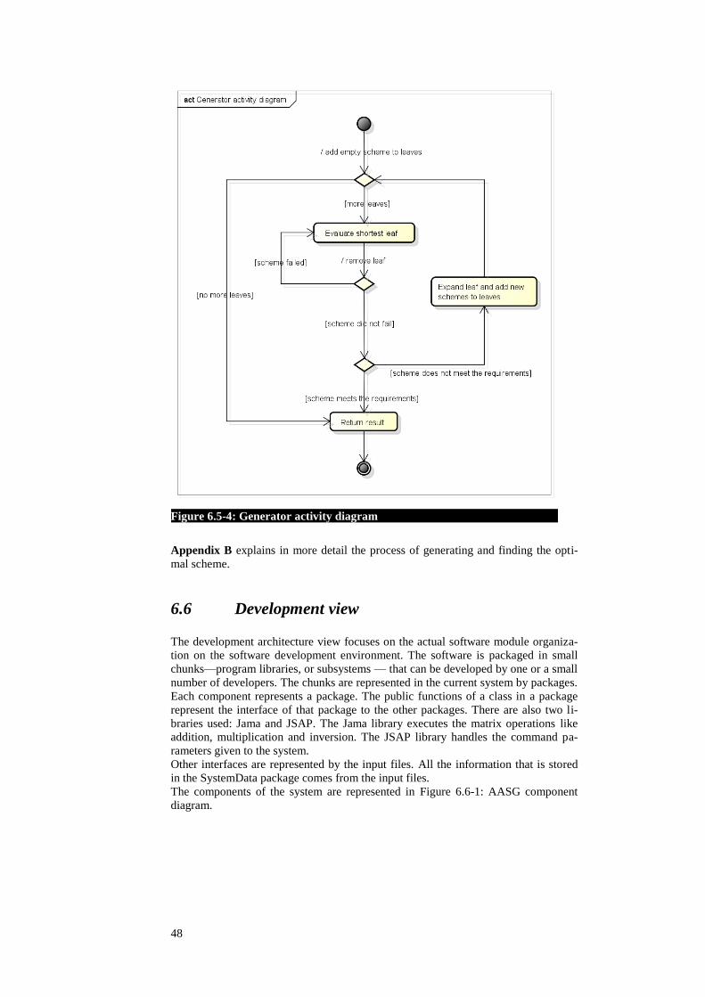
6.5.2. Generator view
The generator is responsible for determining the fastest executing scheme that meets
the accuracy and robustness specifications. These means that it needs to generate and
evaluate new schemes in order to find the optimal one. In order to determine which
scheme is optimal; the search starts from the fastest execution scheme, which is at
start the scheme with no scheme actions (model or scan actions). The generator then
checks if this scheme meets the requirements. If it meets the requirements than the
generator can stop because it found the optimal scheme, otherwise it needs to expand
the scheme by adding one more action. Adding one action means creating a set of
new schemes which are added to the search pool. The next scheme that is then evalu-
ated is the scheme with the shortest execution time from the updated scheme pool.
The process is repeated until an optimal scheme is found or until a maximum of
scheme actions is reached. The process is described in both Figure 6.5-3: Generator
sequence diagram and in Figure 6.5-4: Generator activity diagram.
Figure 6.5-2: Evaluator activity diagram
47
Figure 6.5-3: Generator sequence diagram
48
Appendix B explains in more detail the process of generating and finding the opti-
mal scheme.
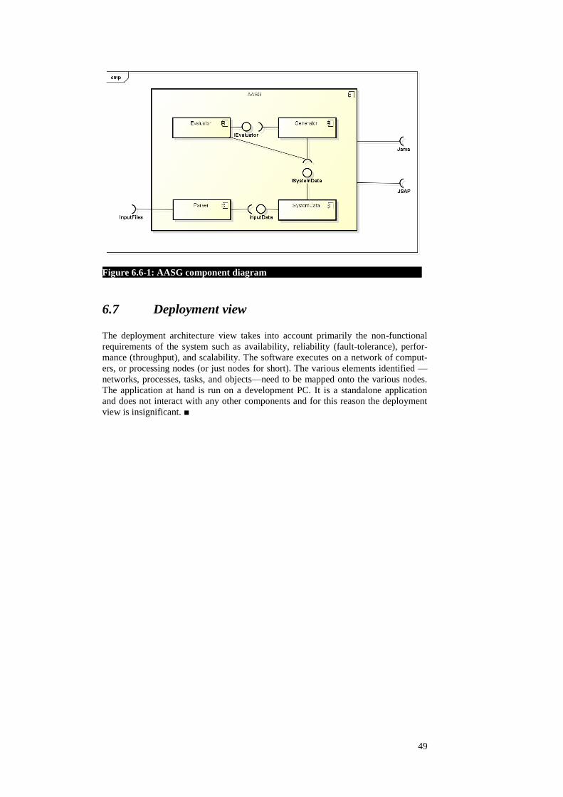
6.6 Development view
The development architecture view focuses on the actual software module organiza-
tion on the software development environment. The software is packaged in small
chunks—program libraries, or subsystems — that can be developed by one or a small
number of developers. The chunks are represented in the current system by packages.
Each component represents a package. The public functions of a class in a package
represent the interface of that package to the other packages. There are also two li-
braries used: Jama and JSAP. The Jama library executes the matrix operations like
addition, multiplication and inversion. The JSAP library handles the command pa-
rameters given to the system.
Other interfaces are represented by the input files. All the information that is stored
in the SystemData package comes from the input files.
The components of the system are represented in Figure 6.6-1: AASG component
diagram.
Figure 6.5-4: Generator activity diagram
49
6.7 Deployment view
The deployment architecture view takes into account primarily the non-functional
requirements of the system such as availability, reliability (fault-tolerance), perfor-
mance (throughput), and scalability. The software executes on a network of comput-
ers, or processing nodes (or just nodes for short). The various elements identified —
networks, processes, tasks, and objects—need to be mapped onto the various nodes.
The application at hand is run on a development PC. It is a standalone application
and does not interact with any other components and for this reason the deployment
view is insignificant. ■
Figure 6.6-1: AASG component diagram

51
7.Conclusions
In this chapter we make a summary of the results achieved with this assignment,
draw conclusions, check if the research questions were answered and talk about fu-
ture work.
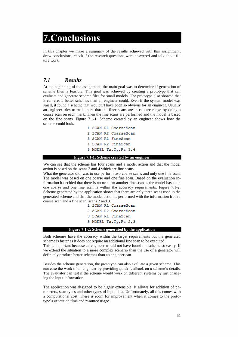
7.1 Results At the beginning of the assignment, the main goal was to determine if generation of
scheme files is feasible. This goal was achieved by creating a prototype that can
evaluate and generate scheme files for small models. The prototype also showed that
it can create better schemes than an engineer could. Even if the system model was
small, it found a scheme that wouldn‘t have been so obvious for an engineer. Usually
an engineer tries to make sure that the finer scans are in capture range by doing a
coarse scan on each mark. Then the fine scans are performed and the model is based
on the fine scans. Figure 7.1-1: Scheme created by an engineer shows how the
scheme could look.
Figure 7.1-1: Scheme created by an engineer
We can see that the scheme has four scans and a model action and that the model
action is based on the scans 3 and 4 which are fine scans.
What the generator did, was to use perform two coarse scans and only one fine scan.
The model was based on one coarse and one fine scan. Based on the evaluation in-
formation it decided that there is no need for another fine scan as the model based on
one coarse and one fine scan is within the accuracy requirements. Figure 7.1-2:
Scheme generated by the application shows that there are only three scans used in the
generated scheme and that the model action is performed with the information from a
coarse scan and a fine scan, scans 2 and 3.
Figure 7.1-2: Scheme generated by the application
Both schemes have the accuracy within the target requirements but the generated
scheme is faster as it does not require an additional fine scan to be executed.
This is important because an engineer would not have found the scheme so easily. If
we extend the situation to a more complex scenario than the use of a generator will
definitely produce better schemes than an engineer can.
Besides the scheme generation, the prototype can also evaluate a given scheme. This
can ease the work of an engineer by providing quick feedback on a scheme‘s details.
The evaluator can test if the scheme would work on different systems by just chang-
ing the input information.
The application was designed to be highly extensible. It allows for addition of pa-
rameters, scan types and other types of input data. Unfortunately, all this comes with
a computational cost. There is room for improvement when it comes to the proto-
type‘s execution time and resource usage.

52
7.2 Answered research questions In the beginning of the project, a set of research questions were formulated. The pur-
pose of research questions was to quantify the results of the project. These questions
are answered in the subchapters below.
7.2.1. Feasibility research questions
The creation of the prototype answered the feasibility research questions. Such an
application can be created as the prototype proves it. If we look at the small model,
the results are given in a relatively short period of time (several minutes) but the
scalability of the application is still unknown. The execution time can increase expo-
nentially based on the number of parameters, scan types, accuracy requirements, etc.
This means that further investigation is required.
The prototype also shows that overlay and focus can easily be used as input data for
the generator. The reason for this is that the evaluator already has enough information
about the system to generate the overlay and focus properties for a scheme. This
means that the generator only needs to define a comparison method that will identify
the better scheme based on the overlay and focus properties.
In the previous subchapter we showed that the prototype can generate better schemes
than an engineer thus it answers the related research question. As the complexity of
the system increases, it is harder for the engineer to compute an optimal scheme.
Related to the generation time of a scheme, we cannot say if it falls in an acceptable
time frame as the model we tested upon is relatively small and does not support all
the features. However, from the information that we gathered, the current prototype
takes a more than a day to generate complex schemes.
The table below shows which feasibility questions were answered.
Table 7.2-1: Feasibility research questions
Feasibility
Answer Question
Yes Is it possible to generate sequences for alignment given the measure-
ment types and accuracies, mechanical tolerances and the model that
relates the two?
Not known Does the duration of the sequence generation fall in an acceptable time
frame (few days)?
Yes Is it possible to have overlay and focus as input parameters for the
generator?
Yes Does the generated scheme improve the scheme generated by an ex-
pert?
7.2.2. Scalability research questions
For the scalability research questions, Table 7.2-2: Scalability research questions, a
few tests were performed. The tests were performed on an Intel Core i5 CPU which
has four cores running at 3.2 GHz frequency running on a Windows 7 with 64-bit
operating system which has 8GB RAM memory. The java virtual machine used in
the tests had 10GB virtual memory.
Because the prototype does not accept overlay and focus as input parameters we can
say that the first scalability question is not answered.
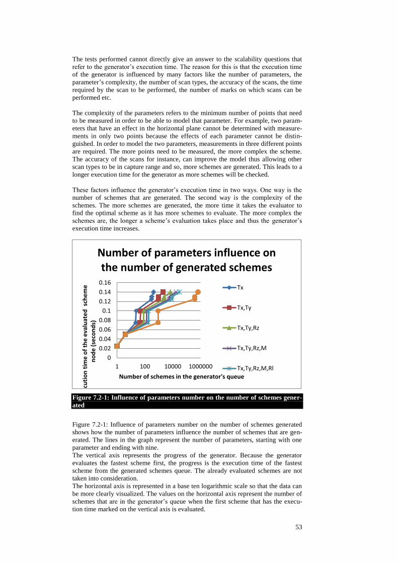
53
The tests performed cannot directly give an answer to the scalability questions that
refer to the generator‘s execution time. The reason for this is that the execution time
of the generator is influenced by many factors like the number of parameters, the
parameter‘s complexity, the number of scan types, the accuracy of the scans, the time
required by the scan to be performed, the number of marks on which scans can be
performed etc.
The complexity of the parameters refers to the minimum number of points that need
to be measured in order to be able to model that parameter. For example, two param-
eters that have an effect in the horizontal plane cannot be determined with measure-
ments in only two points because the effects of each parameter cannot be distin-
guished. In order to model the two parameters, measurements in three different points
are required. The more points need to be measured, the more complex the scheme.
The accuracy of the scans for instance, can improve the model thus allowing other
scan types to be in capture range and so, more schemes are generated. This leads to a
longer execution time for the generator as more schemes will be checked.
These factors influence the generator‘s execution time in two ways. One way is the
number of schemes that are generated. The second way is the complexity of the
schemes. The more schemes are generated, the more time it takes the evaluator to
find the optimal scheme as it has more schemes to evaluate. The more complex the
schemes are, the longer a scheme‘s evaluation takes place and thus the generator‘s
execution time increases.
Figure 7.2-1: Influence of parameters number on the number of schemes gener-
ated
Figure 7.2-1: Influence of parameters number on the number of schemes generated
shows how the number of parameters influence the number of schemes that are gen-
erated. The lines in the graph represent the number of parameters, starting with one
parameter and ending with nine.
The vertical axis represents the progress of the generator. Because the generator
evaluates the fastest scheme first, the progress is the execution time of the fastest
scheme from the generated schemes queue. The already evaluated schemes are not
taken into consideration.
The horizontal axis is represented in a base ten logarithmic scale so that the data can
be more clearly visualized. The values on the horizontal axis represent the number of
schemes that are in the generator‘s queue when the first scheme that has the execu-
tion time marked on the vertical axis is evaluated.
0
0.02
0.04
0.06
0.08
0.1
0.12
0.14
0.16
1 100 10000 1000000
Exe
cuti
on
tim
e o
f th
e e
valu
ate
d s
che
me
n
od
e (
seco
nd
s)
Number of schemes in the generator's queue
Number of parameters influence on the number of generated schemes
Tx
Tx,Ty
Tx,Ty,Rz
Tx,Ty,Rz,M
Tx,Ty,Rz,M,Rl

54
The conclusion that can be drawn from the graph is that the number of generated
schemes increases drastically with the increase of the number of parameters. This
also means that the execution time of the generator increases very fast once the num-
ber of parameters is increased.
Figure 7.2-2: Influence of the scan types on the number of generated schemes
In Figure 7.2-2: Influence of the scan types on the number of generated schemes is
shown how the scan types used influence the number of generated schemes. The axes
in the graph are the same as the ones in Figure 7.2-1: Influence of parameters number
on the number of schemes generated. The horizontal axis however, is no longer a
logarithmical one. The lines in the graph below represent the number of scan types
used, starting with one and ending with three. Like in the number of parameters case,
the increase of scan types used produces an increase in the number of generated
schemes. The effect is increased as the generator evaluates more schemes.
Both Figure 7.2-1: Influence of parameters number on the number of schemes gener-
ated and Figure 7.2-2: Influence of the scan types on the number of generated
schemes show how the number of schemes generated increases the generator‘s exe-
cution time. Indirectly, they answer the scalability questions that refer to the influ-
ence of the number of parameters and scan types on the generator‘s execution time.
Looking at the generator‘s behavior, increasing the number of parameters or the
number of measurement types will determine an increase in the execution time of the
generator.
The scalability tests have also shown that when using the generator, the biggest
amount of time is used to evaluate the schemes and not to generate new ones. The
evaluation time represents more than 80% of the total execution time of the genera-
tor. This explains why the number of generated schemes has such a big influence on
the generator‘s execution time.
The evaluation time of a scheme depends on the number of scenarios that need to be
created to assess that scheme. Figure 7.2-3: Influence of the number of scenarios on a
scheme's evaluation time shows the relation between a scheme‘s number of scenarios
and the time needed to evaluate that scheme. The number of scenarios is shown on
the horizontal axis and the execution time for the number of scenarios is shown on
0
0.02
0.04
0.06
0.08
0.1
0.12
0.14
0.16
0 1000000 2000000 3000000
Exe
cuti
on
tim
e o
f th
e e
valu
ate
d s
che
me
no
de
(s
eco
nd
s)
Number of schemes in the generator's queue
Number of scan types influence on the number of generated schemes
RatioXY_coarse
RatioXY_coarse,RatioXY_fine
RatioXY_coarse,RatioXY_fine,FineHorVert

55
the vertical axis. The graph axes are presented in a logarithmic scale for better visual-
ization reasons.
Figure 7.2-3: Influence of the number of scenarios on a scheme's evaluation time
Because the number of parameters and scan types increase the complexity of a
scheme, this graph also indirectly shows how the execution time of the generator is
influenced by these factors.
The evaluator‘s behavior shows that increasing the number of parameters or the
number of measurement types will also determine an increase in the generator‘s exe-
cution time.
To answer the additional research questions about software extension, adding new
parameters and new scan types takes very low effort. The reason behind this is the
fact that the architecture provides great extendibility. Adding or removing parame-
ters, scan types or marks, requires only the change of the input data. The time con-
suming part of adding new parameters is to create the formulas that describe the ef-
fect that the parameter has on the system. The formulas are then introduced in the
design matrix.
An overview of the answered scalability research question is shown in the table be-
low.
Table 7.2-2: Scalability research questions
Scalability
Answered Question
No How does the change of accuracy parameters to overlay and focus in-
fluence (time) the scheme generator?
Yes How is the execution time of the generator influenced by the number
of measurement types? (Predict scalability based on extension execu-
tion time and implementation time)
Yes How is the execution time of the generator influenced by the number
of modeled parameters? (Predict scalability based on extension execu-
tion time and implementation time)
Yes How much time and man hours are needed to add a new measurement
type/ model parameter? (Predict scalability based on extension execu-
tion time and implementation time)
0.01
0.1
1
10
100
1000
10000
100000
1 10 100 1000 10000 100000 1000000
Exe
cuti
on
tim
e (
seco
nd
s)
Number of scenarios
Number of scenarios vs evaluation time

56
No Is there tradeoff between generation time and scheme execution time?
If yes, what is it?
7.3 Future work The prototype gave good insight to what kind of benefits an application like this can
bring to the reticle align process. In order to create an application that will generate
schemes future work is required. The future work can be split in three categories:
functionality improvements, performance improvements and different approaches.
The functionality improvements refer to the fact that the current prototype generates
schemes only for a small model and with a small set of features. In order to reach full
reticle alignment, more features need to be supported. Among these features, the
most notable ones are:
The parallel scanning which allows for two scans to be performed in paral-
lel on two different marks. This means that the execution time of the
scheme that uses parallel scanning will be shorten and thus be more effec-
tive. Introducing the feature will probably have a high impact on the current
architecture as it requires changes in both the Evaluator and Generator
components.
The non-telecentricity effect which is the correction for an error introduced
by the lens when the distance between the reticle and the wafer changes.
The feature will probably have a low impact and might only need testing as
the architecture allows for model changes which in turn incorporate the
non-telecentricity properties.
The addition of a second TIS plate which means adding more options to the
scans which will increase in the scheme‘s precision. The impact of the fea-
ture is considered to be medium because the current approach does not take
into consideration the plate where the scan is performed.
Besides the functionality improvement, the current prototype also requires perfor-
mance improvements. As mention in the 7.2 subchapter above, the main bottleneck
is the Evaluator as it requires more than 80% of the generation time. The bottleneck
is caused by the large number of scenarios that need to be evaluated and the com-
plexity of the schemes. The bottleneck can be expressed as the amount of resources
needed to evaluate all the scenarios. A solution for this can be processing the scenar-
ios in parallel by making the prototype support threads and by dividing the computa-
tional work to multiple CPUs. Furthermore, a computational computer grid can be
used to decrease the time needed to evaluate schemes. The advantage of this ap-
proach is that the evaluation time will decrease. The improvement should be more
effective for bigger, more complex schemes as the scenarios number is higher. More
investigation is required as for multiple CPUs there is still a memory challenge and
on the computer grid the communication between the computers must be taken into
account as well as the hardware costs.
Another method to reduce the evaluation time is to be able to save the state of an
evaluation. The reason behind this is the fact that the generated schemes have a lot of
scheme actions in common. From Appendix B we know that the search space of the
generator can be represented as a tree and the difference between a scheme and its
parent is one additional scheme action. Knowing the evaluation state of the parent
scheme allows us to avoid evaluating all the scheme actions on the current scheme
and instead continue the evaluation for the one additional scheme action thus having
a smaller evaluation time. The advantage of this method is the decreased evaluation
time and resource consumption for evaluation. As disadvantages, we do not know if
the saving of an evaluation state is possible and how big is the amount of resources
needed for this action.
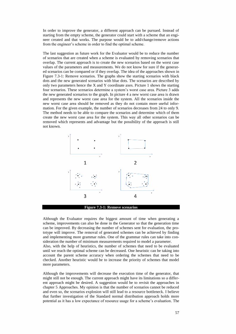
57
In order to improve the generator, a different approach can be pursued. Instead of
starting from the empty scheme, the generator could start with a scheme that an engi-
neer created and that works. The purpose would be to add/change/remove actions
from the engineer‘s scheme in order to find the optimal scheme.
The last suggestion as future work for the Evaluator would be to reduce the number
of scenarios that are created when a scheme is evaluated by removing scenarios that
overlap. The current approach is to create the new scenarios based on the worst case
values of the parameters and measurements. We do not know for sure if the generat-
ed scenarios can be compared or if they overlap. The idea of the approaches shown in
Figure 7.3-1: Remove scenarios. The graphs show the starting scenarios with black
dots and the new generated scenarios with blue dots. The scenarios are described by
only two parameters hence the X and Y coordinate axes. Picture 1 shows the starting
four scenarios. These scenarios determine a system‘s worst case area. Picture 3 adds
the new generated scenarios to the graph. In picture 4 a new worst case area is drawn
and represents the new worst case area for the system. All the scenarios inside the
new worst case area should be removed as they do not contain more useful infor-
mation. For the given example, the number of scenarios decreases from 24 to only 9.
The method needs to be able to compare the scenarios and determine which of them
create the new worst case area for the system. This way all other scenarios can be
removed which represents and advantage but the possibility of the approach is still
not known.
Figure 7.3-1: Remove scenarios
Although the Evaluator requires the biggest amount of time when generating a
scheme, improvements can also be done in the Generator so that the generation time
can be improved. By decreasing the number of schemes sent for evaluation, the pro-
totype will improve. The removal of generated schemes can be achieved by finding
and implementing more grammar rules. One of the grammar rules can take into con-
sideration the number of minimum measurements required to model a parameter.
Also, with the help of heuristics, the number of schemes that need to be evaluated
until we reach the optimal scheme can be decreased. One heuristic can be taking into
account the parent scheme accuracy when ordering the schemes that need to be
checked. Another heuristic would be to increase the priority of schemes that model
more parameters.
Although the improvements will decrease the execution time of the generator, that
might still not be enough. The current approach might have its limitations so a differ-
ent approach might be desired. A suggestion would be to revisit the approaches in
chapter 5 Approaches. My opinion is that the number of scenarios cannot be reduced
and even so, the scenarios explosion will still lead to a resource bottleneck. I believe
that further investigation of the Standard normal distribution approach holds more
potential as it has a low expectance of resource usage for a scheme‘s evaluation. The

58
reason for this is that although the operations with the normal distribution algebra
will be more complex, all the current worst case scenarios will be compressed into
only one. As explained in subchapter 5.2 , the probability function that will repre-
sent the worst case scenario will not be a normal distribution. This way the resource
usage should be manageable. The normal distribution algebra should be reanalyzed to
determine the complexity of its usage. It might also be possible that the normal dis-
tribution is not the key but a different type of distribution might be able to solve the
algebra problem. For this, it should be taken into consideration that continuous distri-
butions can provide lossless algebra, but with potentially infinite complexity while
the discrete distribution can only offer lossy algebra, but can provide finite (and con-
figurable) complexity.
As a last suggestion, I believe that the focus of the project should be the Evaluator
component as it holds the biggest computational part of the application. ■

59
8.Project Management
In this chapter, we discuss the management process involved in fulfilling this project.
In section 8.1 we discuss about the initial project planning and the end results. Sec-
tion 8.2 talks about the risks of the project.
8.1 Milestone Trend Analysis In the beginning of the project a project plan was made. The plan included the fol-
lowing functionality and estimation time:
Objective Estimation
Welcome @ASML 2 weeks
Learning milestone 1 2 weeks
Learning milestone 2 2 weeks
First evaluator 4 weeks
First generator 6 weeks
Extension: 3 dimensions 2 weeks
Extension: Specification 2 weeks
Extension: Non-telecentricity 4 weeks
Extension: Parallel scans 2 weeks
Full reticle align 4 weeks
Documentation 4 weeks
Holiday 2 weeks
Everything went according to plan until the investigation for the First evaluator start-
ed. This showed that the complexity of the problem at hand is not as it was thought
initially and the planning needed to be changed. The decision process was an easy
one because at the start of the project a priority of the features was decided.
Figure 8.1-1: MTA graph shows both the initial milestone planning and the delivery
time. The investigation and complexity delayed both the evaluator and the generator
leaving almost no time for the extensions. Some of the extensions like 3 dimensions
and non-telecentricity were incorporated in the application design. The milestones
that were not completed are not shown in the chart. The Improvements milestone was
added after the prototype was created. This milestone tries to answer the scalability
research questions and bring improvements to the prototype.

60
8.2 Risks management
Table 8.2-1: Potential risks presents the potential risk of the project along with their
contingency and mitigation strategies.
Table 8.2-1: Potential risks
Risks
Risk type Risk name Impact
level
Contingency
strategy
Mitigation
strategy
Process
Experts are una-
vailable
because of
scheduling
problems.
Low
Gather relevant
information
from experts as
soon as possi-
ble.
Focus on other
pressing issues
until
the experts are
available again.
Arrange meet-
ings in advance.
Trainee is ill for
more
than a couple of
days
Medium
Keep a small
buffer slot
for emergen-
cies.
Negotiate re-
quirements
with the
stakeholders.
Not all require-
ments
can be completed
by
the stipulated
deadlines.
High
Be aware of the
project pro-
gress. Monitor
the back-logs
and delays and
negotiate dead-
lines. Make
stakeholders
Negotiate fea-
tures
and deliverables
with the stake-
holders.
2012-01-04
2012-02-01
2012-02-29
2012-03-28
2012-04-25
2012-05-23
2012-06-20
2012-07-18
2012-08-15
2012-09-12
2012-10-10Documentation2012-09-07Improvements 2012-08-07
Firstgenerator2012-04-20Firstevaluator2012-03-09Learningmilestone2 2012-02-10Learningmilestone1 2012-01-29Welcome@ASML2012-01-15ProjectStart2012-01-04
Figure 8.1-1: MTA graph
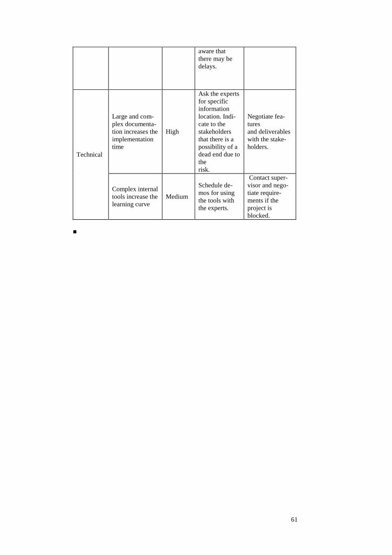
61
aware that
there may be
delays.
Technical
Large and com-
plex documenta-
tion increases the
implementation
time
High
Ask the experts
for specific
information
location. Indi-
cate to the
stakeholders
that there is a
possibility of a
dead end due to
the
risk.
Negotiate fea-
tures
and deliverables
with the stake-
holders.
Complex internal
tools increase the
learning curve
Medium
Schedule de-
mos for using
the tools with
the experts.
Contact super-
visor and nego-
tiate require-
ments if the
project is
blocked.
■

63
9.Project Retrospective
In this chapter, a set of good practices will be mentioned followed by an end of the
project revision of the design competencies.
9.1 Good practices The AASG assignment helped employ the technical and non-technical knowledge
gained during the OOTI programme. Along with this knowledge, there were several
good practices that made a positive impact on the project:
PSGM Monthly project steering group meetings helped keep the most important stakehold-
ers informed on the latest progress and future plans. Also is a very good way of get-
ting feedback and new ideas. Some extra meetings with the TU/e supervisor were
scheduled in the beginning of the project so that he can be better informed about the
project itself and my progress and plan.
Company supervisors At the beginning of the project there were two company supervisors appointed to my
assignment. I found this to be very helpful and I would strongly recommend it for
any project. Even though an extra supervisor is not appointed in the beginning, do
your best in finding another person in the company that can attend all the meetings
and be as informed as your appointed supervisor. This will not only guarantee a
back-up person in case of your appointed supervisor is ill or on holiday but also will
give another perspective in the weekly meetings.
Weekly meetings The weekly meetings with the company supervisors are the most important ones for
the entire duration of the project. In my case we met twice per week. As a good prac-
tice I would say that is better to schedule the meetings at the beginning of the project.
It is easier to cancel a meeting than setting up one as everybody in the company is
very busy. Plan the meetings in the beginning and schedule two meetings per week if
the schedule of the supervisors allows it.
9.2 Design competencies revisited In section 4.5 we mentioned three design competencies that were relevant and two
design competencies that were not relevant in the context of the AASG project. We
revisit these competencies in this section to check their fulfillment.
Realizability In chapter 6, the design of the application is depicted. This confirms that a prototype
was created. Because the prototype was created for a small model, there still remains
the question if the prototype is scalable.
Genericity The use of the Strategy Patterns allows new data to be added to the system, which
means that the system is scalable. Furthermore, the layered architecture provides top
down accessibility and thus promoting the reusability the system components.

64
Functionality
The purpose of the assignment was to create an application that eases the work of an
engineer by generating a new scheme, given a set of requirements, or by providing
feedback on a scheme created by the engineer. If we consider that the engineer will
work with the complete model of the system, than the functionality requirement was
not met. However, for a small model, the functionality competency is met.■

65
Appendix A
Evaluator algorithm description 1. Input data
The data that is needed before starting the evaluation is:
The design matrix which gives the relationship between the parameters of
the system and the measured values.
The mechanical tolerances of the system which are translated into the sys-
tem‘s parameters.
The scheme file that gives the sequence of scan actions and model actions.
The mark information that is required for a scan action.
The mechanical tolerances are given as a range. This means that the parameters are
ranges as well, having a lower and upper value. These lower and upper values deter-
mine the worst case scenarios for the given parameter.
2. Algorithm overview The evaluator‘s purpose is to analyze each action in a scheme file and to create a re-
sult based on the analysis. A scheme file is a sequence of two kinds of scheme ac-
tions, scan actions (SA) and model actions (MA). The equation below is defined with
the Extended Backus–Naur form [8].
*)|(: MASASCHEME
Equation 1
The scan action gives the actual position of a mark with a precision determined by
the scan‘s accuracy. A scan action can be invalid if the mark, on which the scan is
performed, is outside the scan‘s capture range.
The model action computes the new values of a set of parameters based on the in-
formation from the scans. A model action can also be invalid if the information from
the scans is not sufficient to compute the parameters.
The result of evaluating a scheme can be valid or invalid. An invalid scheme is a
scheme that has at least one failed scan or model action.
In order for the algorithm to evaluate the scan and model actions, it needs to have
knowledge about two systems: the real world system and the software system. The
real world system (RWS) is the actual machine; it is described by a vector of trans-
formation parameters (
) and a symbolic design matrix (D).
),( DRWS
Equation 2
A transformation parameter describes an aspect of the state of the system that is used
to calculate setpoints for the reticle and/or wafer stage. Examples are the rotation and
translation of the reticle. The design matrix describes the relation between a vector of
transformation parameters ( p
) and a vector of measurements ( m
); multiplying the
matrix with a vector of transformation parameters results in a vector of measure-
ments. Because some transformation parameters depend on other transformation pa-
rameters, the design matrix is dependent on the vector of transformation parameters.
Also, the design matrix is constructed based on the scan data ( ) used for the scan.
Thus we have the following relationship:
ppDm
*),(
Equation 3

66
Where p
is a general representation of a vector of transformation parameters and
is the scan data used for the scan.
The
values never change as they are the values in the real machine.
is the vec-
tor of transformation parameters of the real machine.
The software system (SS) is what the software (TWINSCAN) thinks the real system
looks like. It is characterized by the software vector of transformation parameters (
) and the same design matrix (D) as in the case of the real machine system.
),( DSS
Equation 4
The scan data is the same as in the real system case.
For the software system to accurately describe the real system, the values of
must
be as close as possible to the values of
.
When a scheme needs to be evaluated, the evaluator does not receive
or
as input
parameters. The only information that it receives about the system is the design ma-
trix D and the worst case values that the parameters in
might have ( w
). The w
vector contains for each parameter in
a worst case lower and upper value.
),(
...
),(
),(
upperlower
upper
2
lower
2
upper
1
lower
1
nn
w
Equation 5
Where1 ,
2 … n are the parameters of
.
A system that is defined only by w
cannot be evaluated. Because the effect of each
parameter in w
on the measurement is described by a linear function, we can formu-
late a conclusion about a system defined by w
if we evaluate all the systems that
have as parameters in
the upper and lower values of the parameters in w
. In other
words, the space of values defined by w
can be evaluated if we evaluate only the
borders of that space. In Figure 1, it suffices to evaluate the systems in points A, B, C
and D in order to formulate a conclusion for the space defined by A, B, C and D.
Figure 9.2-1: The space of a system defined by a w that has only two parameters
For this reason, we introduce the notion of scenarios. A scenario defines a Twinscan
machine. It is characterized by a vector of transformation parameters for the real sys-
67
tem (
) and a vector of transformation parameters for the software system (
). A
scenario A that is characterized by the vectors A
and A
can be written as (
A
, A
).
A worst-case scenario is a scenario that describes a worst-case situation of the sys-
tem. It has as
a combination of lower or upper value for each of the parameters in
w
. Therefore, for each system described by w
we have a number of n2 worst-case
scenarios that will evaluate it, where n is the number of parameters.
Because a scenario is defined by both
and
, and we have information only on
,
we need to estimate the values for
in order to evaluate the scenarios. For the sim-
ple prototype we consider the values of
to be the complement of the values of
in
relation with w
. In w
, we consider the complement of a parameter‘s lower value to
be the parameter‘s upper value. Ex: if the parameter in
takes the lower value of
that parameter in w
, then the same parameter in
will take the upper value of that
parameter in w
.
Other possibilities for the values of
might be: having them given as input, compu-
ting them from the values of
by adding a calibration noise or by taking the average
of the upper and lower values of w
. These alternatives will not be considered in this
document.
After defining the scenarios based on w
, the scheme file can be evaluated.
3. Algorithm components The Evaluator must go through the list of actions in the scheme file and either vali-
dates a scan action or computes the new parameter values for a model action and at
the end computes a result. This is done by three components: validate scans compo-
nent, update parameters component and the compute result component.
Validate scans (scan action)
The first step of the algorithm is to check if the scans from the scheme files are in
capture range. In order to do this it needs the real system measurements vector ( m
),
the software system measurements vector ( m
) and the scan type information ( ).
The software system measurements represent the measurements results that are ex-
pected by the software. The real system measurements and the software system
measurements are computed from the input data using the relationship from Equation
3. The scan type information consists of scan error or scan repro ( ) and scan cap-
ture range ( ). Both of them are tuples, having a minimum and a maximum value.
The first represents the error introduced by the scan and the latter defines the maxi-
mum area in which the scan can do a measurement.
We define m
as being the difference between the real system measurements and the
software system measurements taking into account the error introduced by the scan.
mmm
Equation 6
Where
*),(Dm and
*),(Dm , D is the symbolic design ma-
trix.
The condition that a scan is in capture range is:
m
Equation 7
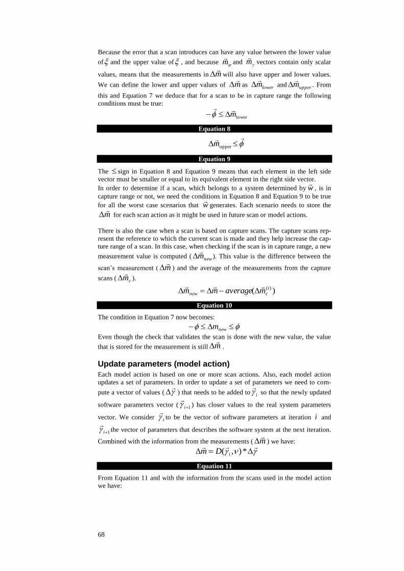
68
Because the error that a scan introduces can have any value between the lower value
of and the upper value of , and because m
and m
vectors contain only scalar
values, means that the measurements in m
will also have upper and lower values.
We can define the lower and upper values of m
as lowerm
and upperm
. From
this and Equation 7 we deduce that for a scan to be in capture range the following
conditions must be true:
lowerm
Equation 8
upperm
Equation 9
The sign in Equation 8 and Equation 9 means that each element in the left side
vector must be smaller or equal to its equivalent element in the right side vector.
In order to determine if a scan, which belongs to a system determined by w
, is in
capture range or not, we need the conditions in Equation 8 and Equation 9 to be true
for all the worst case scenarios that w
generates. Each scenario needs to store the
m
for each scan action as it might be used in future scan or model actions.
There is also the case when a scan is based on capture scans. The capture scans rep-
resent the reference to which the current scan is made and they help increase the cap-
ture range of a scan. In this case, when checking if the scan is in capture range, a new
measurement value is computed ( newm
). This value is the difference between the
scan‘s measurement ( m
) and the average of the measurements from the capture
scans ( cm
).
)( )(i
cnew maveragemm
Equation 10
The condition in Equation 7 now becomes:
newm
Even though the check that validates the scan is done with the new value, the value
that is stored for the measurement is still .
Update parameters (model action)
Each model action is based on one or more scan actions. Also, each model action
updates a set of parameters. In order to update a set of parameters we need to com-
pute a vector of values (
) that needs to be added to i
so that the newly updated
software parameters vector ( 1i
) has closer values to the real system parameters
vector. We consider i
to be the vector of software parameters at iteration i and
1i
the vector of parameters that describes the software system at the next iteration.
Combined with the information from the measurements ( m
) we have:
*),( iDm
Equation 11
From Equation 11 and with the information from the scans used in the model action
we have:
m
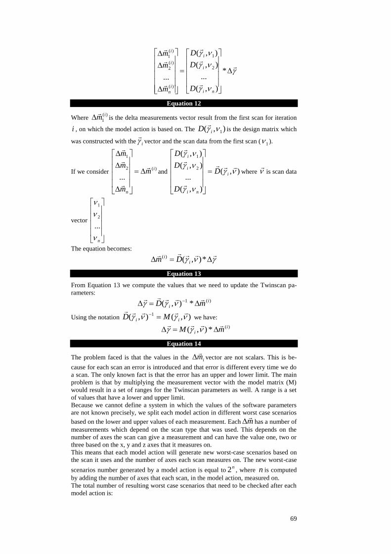
69
*
),(
...
),(
),(
...
2
1
)(
)(
2
)(
1
ni
i
i
i
n
i
i
D
D
D
m
m
m
Equation 12
Where )(
1
im
is the delta measurements vector result from the first scan for iteration
i , on which the model action is based on. The ),( 1 iD
is the design matrix which
was constructed with the i
vector and the scan data from the first scan ( 1 ).
If we consider )(2
1
...
i
n
m
m
m
m
and ),(
),(
...
),(
),(
2
1
i
ni
i
i
D
D
D
D
where
is scan data
vector
n
...
2
1
The equation becomes:
*),()(
i
i Dm
Equation 13
From Equation 13 we compute the values that we need to update the Twinscan pa-
rameters:
)(1 *),( i
i mD
Using the notation ),(),( 1
ii MD we have:
)(*),( i
i mM
Equation 14
The problem faced is that the values in the im
vector are not scalars. This is be-
cause for each scan an error is introduced and that error is different every time we do
a scan. The only known fact is that the error has an upper and lower limit. The main
problem is that by multiplying the measurement vector with the model matrix (M)
would result in a set of ranges for the Twinscan parameters as well. A range is a set
of values that have a lower and upper limit.
Because we cannot define a system in which the values of the software parameters
are not known precisely, we split each model action in different worst case scenarios
based on the lower and upper values of each measurement. Each m
has a number of
measurements which depend on the scan type that was used. This depends on the
number of axes the scan can give a measurement and can have the value one, two or
three based on the x, y and z axes that it measures on.
This means that each model action will generate new worst-case scenarios based on
the scan it uses and the number of axes each scan measures on. The new worst-case
scenarios number generated by a model action is equal ton2 , where n is computed
by adding the number of axes that each scan, in the model action, measured on.
The total number of resulting worst case scenarios that need to be checked after each
model action is:
70
n
wcswcs PrevNew 2*
Equation 15
Where wcsNew is the new number of worst case scenarios that need to be checked,
wcsPrev is the previous number of worst case scenarios that needed to be checked.
Each scenario computes the
values and computes the new software parameters
vector ( 1i
).
ii 1
Equation 16
The measurements of the scans need to be updated as well. This means that from this
point on the measurements for those scans will be scalars instead of ranges. The up-
dated measurements are called residuals ( r
). If these scans are used in a future mod-
el action, these residual values will be used, instead of the m
values.
*),( 1
)(
i
i Dmr
Equation 17
After a model action,
will have the values of 1i
. The result of a model action is
the updated
and the updated measurements r
.
Compute result
After all the actions in the scheme have been evaluated, the accuracy and execution
time of the scheme can be computed.
The execution time of the scheme is given by the number and type of the scheme
actions. The time is not scenario dependent and is the same for all the scenarios.
When computing the accuracy of a scheme file we need to compute the accuracy of
each scenario. Because we have only worst-case scenarios, the accuracy of the
scheme file must also be the worst-case accuracy. This means that the accuracy of the
scheme is the worst accuracy value from all the scenario accuracies.
The accuracy for each scenario ( ) is computed with the following formula:
||max iii
Equation 18
This means that for each parameter in
and in
an absolute difference is computed
and the maximum value will be the scenario‘s accuracy. The scheme file accuracy (
) is:
)(max ss
Equation 19
Where s represents the scenarios iterator.
Scenario explosion 1. Problem analysis
The biggest concern of the algorithm is the number of scenarios that can occur for a
scheme.
The formula for the total number of scenarios is:

71
n
i
iSN1
2*2
Equation 20
Where:
SN = the total number of scenarios
= the number of all the unique modeled parameters in the scheme
n = the number of model actions
i = the number of axes that are used in model action i
The variable depends on the number and type of the scans used in a model action.
For the current alignment schemes RA, which is made up of RA_part1.scheme and
RA_part2.scheme, we have:
= 13
n = 4
M1: = 6, M2: =6, M3: =12, M4: =0
SN = 1.37439E+11
For the current alignment schemes RAvert, which is made up of
RAvert_part1.scheme and RAvert_part2.scheme, we have:
= 16
n = 7
M1: =6, M2: =6, M3: =6, M4: =6,M5: =6, M6: =12, M7:
=0
SN = 2.8823E+17
2. Mitigation strategy Before considering a mitigation strategy, we need to identify the reason for the sce-
nario explosion and the step that leads to it.
The reason is the fact that a scenario cannot be described by a set of ranged software
parameters vector (
). The step that leads to the scenario explosion is the model
action.
A mitigation strategy for the worst-case scenario explosion would be implementing
scenario pruning at every model action. As we are dealing with worst-case scenarios,
the condition for pruning would be that scenario A would be included in a space of
scenarios S and scenario A is limited by scenarios B as the lower limit and scenario C
as the upper limit. Because the pruning is done at a model action the scenarios A, B
and C are all defined by the same real system parameters
. We know that
SCBA ,, and that:
Scenario A is described by the A
vector of software parameters and that
A
A
2
A
1
...
n
A
. Where n is the number of software parameters that define the scenario
andA
1 ,A
2 … A
n are the values of each software parameter. Scenario A can be
defined as (
, A
).
In the same way we define scenarios B and C, (
, B
) and (
, C
).

72
The condition for scenario A to be pruned is:
niiii 1,CAB
Equation 21
This will remove the worst-case scenario A because it would have already been
checked by scenarios B and C. This is only a possible strategy and has not been im-
plemented yet.
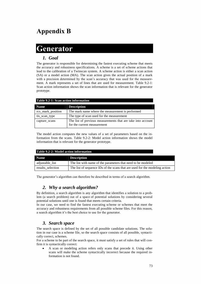
73
Appendix B
Generator 1. Goal
The generator is responsible for determining the fastest executing scheme that meets
the accuracy and robustness specifications. A scheme is a set of scheme actions that
lead to the calibration of a Twinscan system. A scheme action is either a scan action
(SA) or a model action (MA). The scan action gives the actual position of a mark
with a precision determined by the scan‘s accuracy that was used for the measure-
ment. A mark represents a set of lines that are used for measurement. Table 9.2-1:
Scan action information shows the scan information that is relevant for the generator
prototype.
Table 9.2-1: Scan action information
Name Description
rcs_mark_position The mark name where the measurement is performed
tis_scan_type The type of scan used for the measurement
capture_scans The list of previous measurements that are take into account
for the current measurement
The model action computes the new values of a set of parameters based on the in-
formation from the scans. Table 9.2-2: Model action information shows the model
information that is relevant for the generator prototype.
Table 9.2-2: Model action information
Name Description
adjustable_list The list with name of the parameters that need to be modeled
results_selection The list of sequence IDs of the scans that are used for the modeling action
The generator‘s algorithm can therefore be described in terms of a search algorithm.
2. Why a search algorithm? By definition, a search algorithm is any algorithm that identifies a solution to a prob-
lem (a search problem) out of a space of potential solutions by considering several
potential solutions until one is found that meets certain criteria.
In our case, we need to find the fastest executing scheme or schemes that meet the
accuracy and robustness requirements from all possible scheme files. For this reason,
a search algorithm it‘s the best choice to use for the generator.
3. Search space The search space is defined by the set of all possible candidate solutions. The solu-
tion in our case is a scheme file, so the search space consists of all possible, syntacti-
cally correct, schemes.
For a scheme to be part of the search space, it must satisfy a set of rules that will con-
firm it is syntactically correct:
A scan or modeling action refers only scans that precede it. Using other
scans will make the scheme syntactically incorrect because the required in-
formation is not found.

74
A modeling action will not model parameters that are not contained by the
vector that describes the real machine system (
). (See the Evaluator algo-
rithm description) Using other parameters than the ones defined in
will
make the scheme syntactically incorrect.
The number of modeled parameters must be less or equal to the number of
dx, dy and dz information resulted from the capture scans. If the number of
modeled parameters is higher than the number of equations resulted from
the scan information, the system of equations cannot be solved thus the
modeled parameters cannot be computed.
The search space (W ) definition is shown in Equation 22.
schemecorrectllysyntacticaaissWs
Equation 22
With the current definition, the search space is unlimited because there is no bounda-
ry on how many scheme actions a scheme must have. An unlimited search space is
not desired because the search algorithm might not find a solution in a finite period
of time. Therefore, a limit on the number of scheme actions must be imposed so that
it makes the search space finite. This limit will be discussed further in the paper.
We can also define a set of grammar rules that will decrease the search space size by
removing the schemes that add redundancy or are considered inefficient:
A non-empty scheme file must always start with a scan action. The reason
behind this is the fact that a modeling action requires scan actions in order to
model any parameter.
If multiple scans that differ only in accuracy and nothing else are available,
then subsequent modeling or scan actions will only reference the most accu-
rate of these scans. Using scans that have low accuracy will lead to reaching
a lower scheme accuracy level compared to a model action that uses more
accurate scans.
A scan must not be repeated within the same scheme file. Repeating a scan
will only increase the scheme execution time and not the accuracy and the
goal of the scheme is to have high accuracy and small execution time. This
is a consequence of only considering the worst case scenarios. In the real
world, repeating a scan means improving the accuracy of the scan.
A modeling action must not be repeated within the same scheme file. A
modeling action that uses the same scans as capture scans and models the
same parameters will not improve the accuracy of the scheme file but will
increase the execution time.
Once the search space has been defined, we need to define a set of rules that will help
us identify a solution within the search space.
4. Solution selection A solution is considered to be a scheme that is robust and has an accuracy value less
or equal than the specified target accuracy ( accT ). In order to identify the solution
schemes in the search space, we need to define two functions f and g that will de-
termine if a scheme is robust and within the accuracy requirements.
Function f will identify if a scheme is robust or not. This means that f will verify
that each scan action in the scheme file is within capture range and that each model
action can compute its model parameters.

75
robustsfcomputableMArangecaptureinSAsMAsSAWs )(,,,,
Equation 23
Using f on our search space will shrink it to a search space that only contains robust
scheme files. We use theV notation to identify the search space that has only robust
scheme files.
VsrobustsfandWsIf )(
Equation 24
Function g will check the accuracy level of a robust scheme file. The function will
evaluate each scheme file from V and will check if its accuracy level is less or equal
to the specified target accuracy ( accT ). Based on the comparison it will conclude if
the scheme is accurate or not.
INACCURATEACCURATETsaccuracysg acc :?)()(
Equation 25
Function g applied to V will give a space that contains all the scheme files that are
robust and accurate and thus determining the solution space S .
SsACCURATEsgandVsIf )(
Equation 26
Because the goal of the algorithm is to find the fastest executing scheme that is ro-
bust and meets the accuracy requirements, we need to compute the execution time for
each scheme.
We define function Wh : which will return the execution time of the scheme
if the scheme is robust and infinity if the scheme is not robust. The h function will
act as a cost function and will help us choose the optimal solution or solutions from
the solution space.
n
i
i INFINITYnschemActiodurationrobustsfshWs1
:)(?)()(,
Equation 27
Having the three functions, we can now specify the optimal solution space ( O ) as
shown in Equation 28.
OsxhshandSxthenACCURATEsgandrobustsfWsIf )()()()(,
Equation 28
The O space will contain only the scheme files that are robust, within accuracy con-
straints and their execution time is less or equal than any other scheme that is robust
and within the accuracy constraints.
5. Naive search algorithm A first approach on finding the optimal scheme file/files is the naive search algorithm
approach. The goal of the naive search algorithm is to check all the scheme files in
the search space W and identify the scheme files that are robust, within accuracy
specification and have the smallest execution time; the scheme files that create the
O space (Equation 28).
As mentioned in the Search space chapter, a limitation must be set on the number of
scheme actions that a scheme can have. This limitation will guarantee that the search
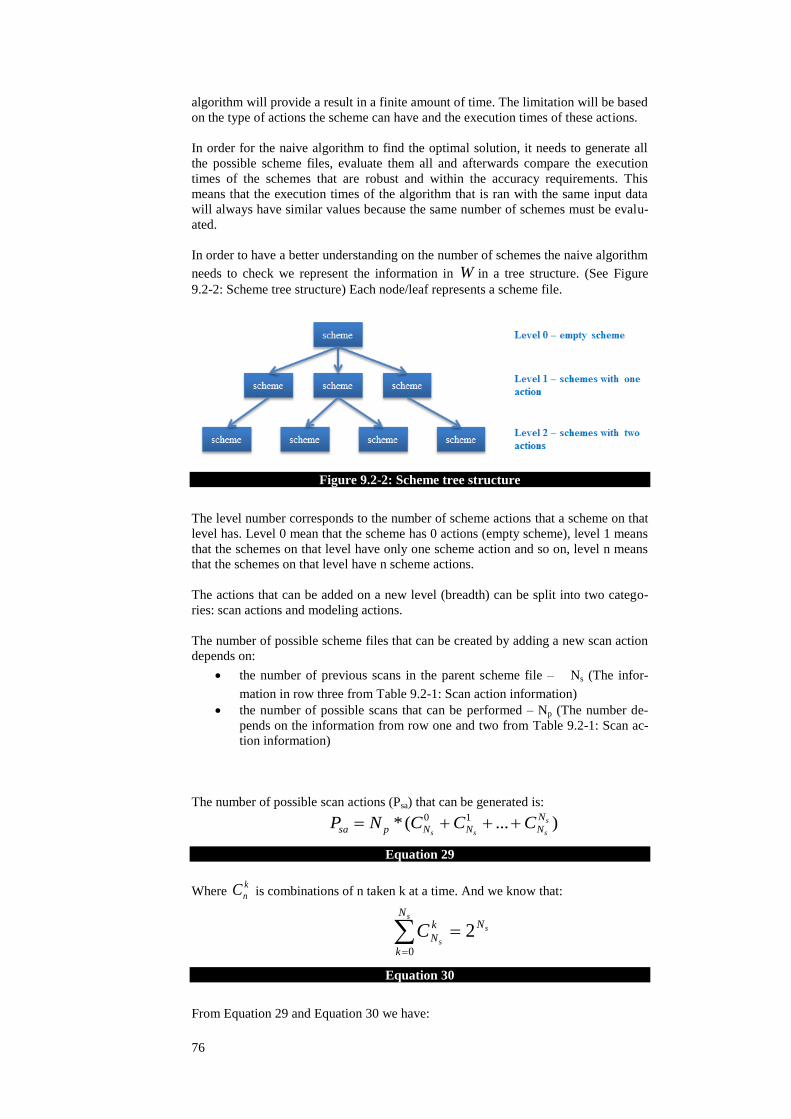
76
algorithm will provide a result in a finite amount of time. The limitation will be based
on the type of actions the scheme can have and the execution times of these actions.
In order for the naive algorithm to find the optimal solution, it needs to generate all
the possible scheme files, evaluate them all and afterwards compare the execution
times of the schemes that are robust and within the accuracy requirements. This
means that the execution times of the algorithm that is ran with the same input data
will always have similar values because the same number of schemes must be evalu-
ated.
In order to have a better understanding on the number of schemes the naive algorithm
needs to check we represent the information in W in a tree structure. (See Figure
9.2-2: Scheme tree structure) Each node/leaf represents a scheme file.
Figure 9.2-2: Scheme tree structure
The level number corresponds to the number of scheme actions that a scheme on that
level has. Level 0 mean that the scheme has 0 actions (empty scheme), level 1 means
that the schemes on that level have only one scheme action and so on, level n means
that the schemes on that level have n scheme actions.
The actions that can be added on a new level (breadth) can be split into two catego-
ries: scan actions and modeling actions.
The number of possible scheme files that can be created by adding a new scan action
depends on:
the number of previous scans in the parent scheme file – Ns (The infor-
mation in row three from Table 9.2-1: Scan action information)
the number of possible scans that can be performed – Np (The number de-
pends on the information from row one and two from Table 9.2-1: Scan ac-
tion information)
The number of possible scan actions (Psa) that can be generated is:
)...(* 10 s
sss
N
NNNpsa CCCNP
Equation 29
Where k
nC is combinations of n taken k at a time. And we know that:
s
s
s
N
k
Nk
NC0
2
Equation 30
From Equation 29 and Equation 30 we have:

77
sN
psa NP 2*
Equation 31
The number of possible scheme files that can be created by adding a new model ac-
tion depends on:
the number of parameters that can be modeled in the system -
the number of scans in the parent scheme file – Ns
The number of possible model actions (Pma) that can be generated is:
sN
maP
2
Equation 32
The value of Pma is a pessimistic value because the actual number depends on the
characteristics of the scans in the scheme file.
The sum of Psa and Pma values define the number of actions that a level can have.
This means that each branch downwards adds a limited number of actions.
The conclusion is that the naive algorithm is very time and resource consuming as it
will evaluate all the schemes even when the optimal scheme has already been found.
6. Improvements The naive algorithm described in the previous chapter will find a solution but not in
the fastest way possible. The number of possible schemes that need to be checked
increases drastically with every level of the scheme tree. This means that a set of im-
provements need to be added in order to get to an optimal solution faster and with
less computation.
Order of search
The order of search method aims at decreasing the algorithm‘s search time by first
checking the possibilities that are closest to the solution.
For the naive algorithm the order of generating new schemes was not important. This
approach will only remember the leaves of the tree and will evaluate and expand one
leaf at a time, the shortest one. Expanding a node means adding only one scheme
action to the list of scheme actions that the node has.
Evaluating and expanding the leaf with the shortest execution time increases the
chances of finding an optimal scheme in a shorter period of time.
The reason for choosing the fastest executing leaf is based on the condition that the
optimal solution must have the shortest execution time from all the accurate and ro-
bust schemes and that adding actions to a scheme will increase its execution time.
Derived from these conditions we can state that each search should start with evaluat-
ing the empty scheme as it always has the shortest execution time and is always ro-
bust.
By using the order of search method, we can improve the naive algorithm by not
checking all the possible schemes that have a bigger execution time than the optimal
solution.
We guarantee an optimal solution is found when at least one solution was found and
there is no other leaf that has a lesser execution time than the time of that solution.
Pruning
Pruning is a technique that is used in search algorithms to reduce the size of the
search space by identifying and removing potential solutions that have a low or no
probability of being a solution.
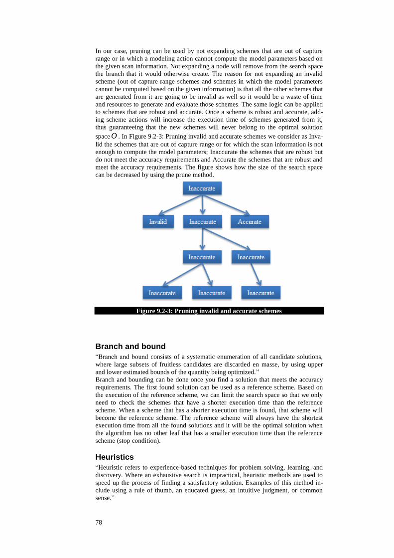
78
In our case, pruning can be used by not expanding schemes that are out of capture
range or in which a modeling action cannot compute the model parameters based on
the given scan information. Not expanding a node will remove from the search space
the branch that it would otherwise create. The reason for not expanding an invalid
scheme (out of capture range schemes and schemes in which the model parameters
cannot be computed based on the given information) is that all the other schemes that
are generated from it are going to be invalid as well so it would be a waste of time
and resources to generate and evaluate those schemes. The same logic can be applied
to schemes that are robust and accurate. Once a scheme is robust and accurate, add-
ing scheme actions will increase the execution time of schemes generated from it,
thus guaranteeing that the new schemes will never belong to the optimal solution
space O . In Figure 9.2-3: Pruning invalid and accurate schemes we consider as Inva-
lid the schemes that are out of capture range or for which the scan information is not
enough to compute the model parameters; Inaccurate the schemes that are robust but
do not meet the accuracy requirements and Accurate the schemes that are robust and
meet the accuracy requirements. The figure shows how the size of the search space
can be decreased by using the prune method.
Figure 9.2-3: Pruning invalid and accurate schemes
Branch and bound
―Branch and bound consists of a systematic enumeration of all candidate solutions,
where large subsets of fruitless candidates are discarded en masse, by using upper
and lower estimated bounds of the quantity being optimized.‖
Branch and bounding can be done once you find a solution that meets the accuracy
requirements. The first found solution can be used as a reference scheme. Based on
the execution of the reference scheme, we can limit the search space so that we only
need to check the schemes that have a shorter execution time than the reference
scheme. When a scheme that has a shorter execution time is found, that scheme will
become the reference scheme. The reference scheme will always have the shortest
execution time from all the found solutions and it will be the optimal solution when
the algorithm has no other leaf that has a smaller execution time than the reference
scheme (stop condition).
Heuristics
―Heuristic refers to experience-based techniques for problem solving, learning, and
discovery. Where an exhaustive search is impractical, heuristic methods are used to
speed up the process of finding a satisfactory solution. Examples of this method in-
clude using a rule of thumb, an educated guess, an intuitive judgment, or common
sense.‖

79
With the use of heuristics, we can further improve the algorithm by better guiding it
towards the optimal solution. In the Order of search improvement, we consider the
nodes with the shortest execution time as being the best choice at the given moment.
If we add the heuristics knowledge to this assumption we can get a shorter path to-
wards an optimal solution.
An example of heuristics is to model the parameters that have a greater impact on
overlay first so that the error that these parameters can introduce in the system is
smaller. The algorithm would take this information into account and will first expand
schemes that have a low execution time and model these parameters.
7. Improved algorithm
The goal of the improved algorithm is to make the naive algorithm more effective.
For this we apply the extension described in the Improvements chapter to the naive
algorithm.
The improved algorithm will starts its search for the optimal solution with the empty
scheme as it is robust and the fastest executing scheme available. If the empty
scheme is not accurate enough, then based on the rules described in the Search space
chapter, it will expand the node that contains the empty scheme by adding only one
more action. The improved algorithm will increase its search base only after it evalu-
ates a leaf. The new added schemes will be generated from the evaluated leaf.
The improved algorithm will always evaluate the leaf that has the shortest execution
time. This will make the search for an optimal scheme more efficient as the first ac-
curate scheme that is found has the smallest execution time. Once a robust and accu-
rate scheme has been found, means that the optimal scheme has been found because
all other leaves have a higher execution time than the found scheme. The improved
algorithm can also use heuristics to decrease the number of generated schemes.
The improvements used for the prototype were the order of search and pruning. The
branch and bound and heuristics improvements were only investigated.


81
Glossary
AASG ASML Alignment Sequence Generator
EUV Extreme Ultraviolet
IC Integrated Circuit
NXE TWINSCAN NXE platform is the industry‘s first production plat-
form for extreme ultraviolet lithography
Photoresist A light-sensitive material used in the photolithography industry
TIS Transmission Image Sensor
TWINSCAN An ASML machine platform that with its unique dual-stage design
allows for non-stop processing: measuring one wafer while imaging
another.
UML Unified Modeling Language


83
Bibliography
[1] "ASML website," [Online]. Available: http://www.asml.com.
[2] "Photolithography," [Online]. Available:
http://en.wikipedia.org/wiki/Photolithography.
[3] "Normal product distribution," [Online]. Available:
http://mathworld.wolfram.com/NormalProductDistribution.html.
[4] "Normal ratio distribution," [Online]. Available:
http://mathworld.wolfram.com/NormalRatioDistribution.html.
[5] Microsoft Patterns & Practices Team, Microsoft® Application Architecture
Guide, 2nd Edition, Microsoft Press, 2009.
[6] P. Kruchten, "Architectural Blueprints—The ―4+1‖ View," IEEE, November
1995.
[7] G. Booch, Object-Oriented Analysis and Design with Applications, Redwood
City, California: Benjamin-Cummings Pub. Co., 1993.
[8] "Extended Backus-Naum Form," [Online]. Available:
http://en.wikipedia.org/wiki/Extended_Backus%E2%80%93Naur_Form.
[9] M. v. d. Horst, "GID Designing ASML's calibration sequence optimizer,"
Internal ASML document, 2011.
[10] M. v. d. Horst, "EPDS NXE Metrology modeling expose (KXMI)," Internal
ASML document, 2010.
[11] R. Bogers and I. Jiménez, "EDS Reticle Align/Reticle Shape Correction,"
Internal ASML document, 2008.


85
About the Authors
Bogdan Mihai Lazăr received his MSc. equivalent degree
from the Polytechnic University of Bucharest, Faculty of
Automatic Control and Computer Science in 2008. In the
same year he started the Master studies in Informatics
Systems for Economic Processes and Resources Man-
agement at the Bucharest Academy of Economic Studies.
He joined in October 2010 the two years PDEng program
at Eindhoven University of Technology and is expected to
graduate in September 2012.
During the university studies he worked in two IT com-
panies in Bucharest, Romania. He gained more than three
years of experience in the IT domain and more than five
years work experience. After his graduation in September
2012 he will be using his knowledge and expertise as a
software engineer at ASML, The Netherlands.