
C. 3
SANDIA REPORTSAND96–2459 • UC-905Unlimited ReleasePrinted October 1996
Aspen: A Microsimulation Model ofthe Economy
N. Basu, R. J. Pryor, T. Quint, T. Arnold
Prepared bySandia National LaboratoriesAlbuquerque, New Mexico 87185 and Livermore, California 94550for the United States Department of Energyunder Contract DE-AC04-94AL85000
Approved for public release; distribution is unlimited.
.
Issued by Sandia National Laboratories, operated for the United StatesDepartment of Energy by Sandia Corporation.
NOTICE: This report was prepared as an account of work sponsored by anagency of the United States Government. Neither the United States Govern-ment nor any agency thereof, nor any of their employees, nor any of theircontractors, subcontractors, or their employees, makes any warranty,express or implied, or assumes any legal liability or responsibility for theaccuracy, completeness, or usefulness of any information, apparatus, prod-uct, or process disclosed, or represents that its use would not infringe pri-vately owned rights. Reference herein to any specific commercial product,process, or service by trade name, trademark, manufacturer, or otherwise,does not necessarily constitute or imply its endorsement, recommendation,or favoring by the United States Government, any agency thereof or any oftheir contractors or subcontractors. The views and opinions expressedherein do not necessarily state or reflect those of the United States Govern-ment, any agency thereof or any of their contractors.
Printed in the United States of America. This report has been reproduceddirectly from the best available copy.
Available to DOE and DOE contractors fromOffice of Scientific and Technical InformationPO BOX 62Oak Ridge, TN 37831
Prices available from (615) 576-8401, FTS 626-8401
Available to the public fromNational Technical Information ServiceUS Department of Commerce5285 Port Royal RdSpring-field, VA 22161
NTIS price codesPrinted copy: A04Microfiche copy AO1
SAND96-2459Unlimited Release
Printed October 1996
Distribution
Category UC-905
ASPEN: A MICROSIMULATION MODELOF THE ECONOMY
N. Basu, R. J. Pryor, T. Quint, T. ArnoldProgram Management Department
Sandia National LaboratoriesAlbuquerque, NM 87185
Abstract
This report presents Aspen. Sandia National Laboratories is developing this new agent-
based macroeconomic simulation model of the U.S. economy. The model is notable
because it allows a large number of individual economic agents to be modeled at a high
level of detail and with a great degree of freedom. Some features of Aspen are (a) a
sophisticated message-passing system that allows individual pairs of agents to
communicate, (b) the use of genetic algorithms to simulate the learning of certain agents,
and (c) a detailed financial sector that includes a banking system and a bond market.
Results from runs of the model are also presented.

Intentionally Left Blank
ii
Nomenclatwe .......................................................................................................................v
htroduction ..........................................................................................................................l
Back~oud ..........................................................................................................................2
Aspen: The Model ...............................................................................................................3
The Mechanics of the Model ............................................................................................................ 3Initializing Values and Creating Parameters ....................................................................4Agents ..............................................................................................................................5
Results and Discussion ......................................................................................................l2
Economic Results ...........................................................................................................l2Run Times and Agent Location .....................................................................................l4GALCS: Ftier Discussion .........................................................................................l5GALCS and Prices: Final Obsenation .........................................................................l6
Conclusion .........................................................................................................................l7
References ..........................................................................................................................l8
APPENDIX A
APPENDIX B
APPENDIX C
Initializing Values and Creating Parmeters ......................................... A-1
Graphs Illustrating Study Results ...........................................................B.l
Run Time Results ...................................................................................c.l

Intentionally Left Blank
iv
Nomenclature
Aspen
CGE
GALCS
GNP
Sandia
(an agent-based simulation model of the U.S. economy)
computable general equilibrium
genetic algorithm learning classifier system
gross national product
Sandia National Laboratories
v

Intentionally Left Blank
vi
ASPEN: A MICROSIMULATION MODELOF THE ECONOMY
Introduction
This paper describes Aspen, a new simulation model of the U.S. economy that SandiaNational Laboratories (Sandia) is developing.1 Aspen runs on Sandia’s massively parallelIntel Paragon computer and is an agent-based Monte-Carlo simulation. Individual agentsin the model represent real-life economic decision-makers. Aggregates of the agents’macroeconomic actions generate macroeconomic quantities of interest.
The building blocks of Aspen are agents, the first of which is the household agent. Thehousehold agent works or collects unemployment or social security for income. Thisagent spends income on four consumer items, contributes to a savings account, or investsin bonds.
Firm agents produce four types of goods. The four types of firm agents are automobilemanufacturers, housing developers, producers of nondurable goods (such as food), andproducers of nondurable goods the consumption of which is income dependent. Eachfirm uses capital equipment in addition to labor to produce goods. Each firm sets pricesby using a genetic algorithm learning classifier system (GALCS). GALCS simulatesfirm-agent learning as the agent develops a pricing strategy.
The single government agent collects income, sales, and payroll tax. Also, this agent runsa social security system, pays unemployment benefits, runs a public sector, and issuesgovernment bonds during a deficit.
Finally, a well developed financial sector includes (a) banks that maintain householdsavings accounts, make consumer and business loans, and invest in bonds; (b) the federalreserve, which may conduct an expansionary or contractionary monetary policy; and (c) afinancial market agent that reconciles demand and supply for bonds among thegovernment, banks, and households.
The model omits certain important factors of the U.S. economy. For example, thedefense industry, service sector, and stock markets are not represented. These elementsare planned for a fiture version of the model. However, when we, the authors, tested theoutcome of various federal monetary policies in the model (see Results and Discussion),the results agreed qualitatively with predictions based on economic theory and practice.
1The model described here is an update of the prototype model described in Pryor-Basu-Quint ( 1996). Inthat paper, this paper’s model is referred to as the developmental model.
1
the results agreed qualitatively with predictions based on economic theory and practice.This result is significant for such a novel simulation technique (especially for use of thegenetic algorithms). Hence, even in its current state, the model has merit.
This paper is organized in three major sections plus a conclusion. The Backgroundsection addresses macroeconomic simulation. Aspen: The Model covers modelmechanics, initializing and creating parameters, and agent descriptions. Results andDiscussion presents economic results, run times, agent location, and GALCS and theirrelationship to price.
Background
A4icrosimzdation of the economy refers to a model that simulates the actions of economicdecision-makers individually and then generates macroeconomic quantities of interest byintegrating those actions. Microsimulation is a relatively new approach; we know of onlytwo such models of the U.S. economy.2 Potentially, Aspen affords several advantagesover traditional techniques (macroeconometric or computable general equilibrium [CGE])of modeling the economy:
(a) The procedure does not require a fictional form for its endogenousrelationships (as macroeconometric and CGE models do). The user hasgreat freedom when modeling individual agent behavior and can model indetail. For example, Aspen simulates the learning of some agents by usinggenetic algorithm learning classifier systems (GALCS) (see Aspen: TheModel). In addition, the effect of certain nonlinear legal, regulatory, and/orpolicy changes (such as in tax law) can be modeled explicitly.
(b) The procedure is individual-agent-based. Therefore, the user must buildmacroeconomic models of the individual decision-maker rather thanmacroeconomic models of markets. Existing rich sources of micro-leveldata are available.
(c) The user can easily model a stochastic element using a simple randomnumber generator.
Until now using macroeconomic simulation had two major disadvantages: First, becausethe technique is so new, minor modeling problems had not been solved, and modelparameter values had not been estimated. Hence, at present this type of model cannotforecast as accurately as a macroeconometric or a CGE model can. Second, tracking
2 One is the Urban Institute Model developed by Guy Orcutt. See Orcutt-Caldwell-Wertheimer 1976. Theother is Robert Bennett and Barbara Bergmann’s Transaction Model (Bennett-Bergmann, 1986).
2
numerous agents-especially if they are modeled in great detail—can require anenormous computing capacity. However, given time and computing facilities such asSandia’s Intel Paragon (currently the nation’s fastest computer), macroeconomicsimulation models should eventually match their classical counterparts in capability andforecasting accuracy.
Aspen: The Model
This section discusses model mechanics, initializing and creating parameters, and theAspen agents (including households, firms, banks, government, the financial market, thefederal reserve, and the realtor and capital-goods producer).
The Mechanics of the Model
In Aspen, decision-makers in the economy are called agents. There are many classes
(types) of agents, which are organized into two groups. The first group includes thoseclasses for which there will be many agents representing them in a calculation. Theseclasses are households, banks, and four types of firms: food producers, other nondurable-goods producers, automobile makers, and housing developers. The second group ofclasses will have only a single agent representing them in a calculation. These classes aregovernment, federal reserve, capital goods producer, and a fnmncial market agent.
Each agent behaves the way a real counterpart of the same type would. Microsimulationtraces the agent’s daily actions (buying food, hiring workers, selling bonds, collectingwelfare payments, conducting open market operations, etc.). Agents in the same classdraw from the same decision rules. For example, if a renter household agent decides tobuy a home, the agent must apply for a 30-year loan. Payments will be at most 35’% ofthe agent’s incomes However, other renter agents may take different actions because (a)they may be in different states (that is, two household agents at a particular time may havedifferent incomes and, therefore, opt for different sized loans); or (b) they may drawdifferent random numbers and decide not to buy a home at all.
The model uses a system of message passing that allows agents to perform actions. Timesequencing is key to message passing. In Aspen, time is divided into discrete periods ordays. Every day is divided into 11 stages. An agent is processed once per stage. This
3 The parameters 30 (year) and 357. can be changed at the discretion of the user during themicrosimulation run. See Initializing Values and Creating Parameters.
3
means the agent (a) reads any incoming messages and acts upon them, then (b) takesallowable independent actions according to that agent’s current status.
Most actions are allowed once at most per day during a specified stage. For instance, anautomaker agent pays income tax only during stage 1 each day. To accomplish this, theautomaker debits an account by the requisite amount and sends a message to thegovernment saying “I’m paying taxes of $x” During processing, the government agentreads the incoming message and credits the automaker’s tax payment of $X.4
More complicated series of actions require a series of messages to be passed. Forexample, if a household decides to buy a new home, the household agent calculates howmuch s/’hecan borrow and sends a message to a bank requesting a mortgage loan. Thebank then reads this message. Based on the information the household sent, the bankagent approves or rejects the loan request. Regardless, the bank sends a message to thehousehold. If the message is “accept,” the household responds to a developer by statingthat the household agent wants to buy a house.
Implementation of the message-passing system is an important computational capability.Aspen is designed to run on the massively parallel Paragon computer; hence, the agents inthe model are distributed among the processing nodes of the computer. Each agent has amessage queue containing incoming messages for the agent to read. When an agent sendsa message, a toolbox routine determines whether the recipient is on the same node. If so,the message is immediately placed in the recipient’s queue. If the recipient is not on thesame node, the message enters a holding area for messages to be routed fi-om the sendernode to the recipient node. At the end of the stage, the holding areas are emptied, and thecontents are shipped in packets to the appropriate nodes. All messages going fi-om oneparticular node to another particular node are placed in the same packet. At the beginningof the next stage, the packets arriving at each node are broken, and their messages aredistributed (using a second toolbox routine) into individual agent queues. When they areprocessed, recipients read the messages (using another toolbox routine).
In this way, each stage has at most only one cross-node communication between a givenpair of nodes. (If no agent on the sending node wishes to send a message to an agent onthe recipient node, no cross-node communication occurs.) Communicating betweennodes on the Paragon requires a significant amount of time and could degrade theperformance of the run.
Initializing Values and Creating Parameters
Many agent decisions in Aspen depend on the agent’s current state. For example, ahouseholder agent’s consumption decisions depend on family size, current income,savings account balance, bond holdings, etc. Certain values must be initialized. When an
4 Every cash debit is balanced by a credit (and vice versa). This provides an accounting check that ensuresthe model runs properly and that the total amount of money in the economy is conserved.
4
Aspen run begins, each household is assigned a savings account balance, an initial bondholding, and an age for the household head. These kinds of assignments are donerandomly using pre-selected distributions. For instance, for initial savings levels eachhousehold draws its value fi-om an exponential distribution with mean $800. In this way,Aspen simulates a heterogeneous population.
For almost any quantity, the user can enter unique values. Otherwise, default values areused.
The above discussion applies also to the numerous parameters of the models, (such as thefi-equency of automobile breakdowns, the length of a standard mortgage, or thepercentage of savings that constitutes the reserve requirement at a bank).
See Appendix A for a list of initialization values and parameters together with respectivedefault values. Default values were used in the runs discussed in the Results andDiscussion section.
Agents
This subsection reviews the decision rules for agents from each of the different classes.Figure 1 illustrates the logical relationships between the various agent classes.
Households (Individuals)Most Aspen agents are households (individuals). Household agents generate most oftheir income through employment. Employers are from one of the four firm types orfi-om banking, real estate, capital goods production, or the government sector. Thehouseholder obtains a job by accepting a job offer message. The employer pays a salaryuntil the householder/employee quits or is fired. If at any time a householder is notemployed, this agent collects a welfare payment from the government. The paymentamount depends on family size. A senior citizen may collect social security payments.Other revenues a householder may generate include interest payments from bonds andsavings accounts as well as shares of company profits (see Firms), The householder paysa flat-rate income tax on all income.
5
AGENT INTERACTIONSIN ASPEN
Taxes
Wage and Profii
lNK-0c %al au-0 -0
vBOND
MARKETDetermines
Bond Price andinterest
vLOAN
MARKETDetermines
Loan InterestUsingG4
T
PRODUCTWK13Determines
Produf3 PriceUsii GAsnd LaborDemand byInventory
Maintainance-u
a au-0 v5 5m Bond demand
and SU@y
~
$
,
.
\
\
--7
+
Labor Demand
L4BORMARKET
DeterminesWage
===--’l 1~ Transfer GOVERNMENTL I wagesPublict%ods
R.-mrl A.rn.rul Iand SU@Y
Figure 1. Aspen Agent Interactions.
6
Thehouseholder consumes fourtypes ofgoods eachday: foodand other nondurablegoods, aswellas goods mdsemices related totrmspotiation mdshelter. A householderagent’s goods consumption is not determined in the usual way; there is no exogenousutility function that is maximized over all feasible consumption bundles. Rather, Aspenuses simulation techniques and reasonable rules of thumb.
Demand for food is assessed daily based on family size. When this demand has beendetermined, the household agent identifies a suitable food firm. The agent first consults alist of food prices; each food firm broadcasts price-per-unit messages daily.
If firm f offers food for price p(f), the household agent buys from this food with aprobability k“~(fj]-q
where q = a given exogenous parameter andk = a normalizing constant.
In words, the lower p(~ is in relation to other firms’ prices, the greater chance thehousehold has of satisfying its demand by buying from f.
A household consumes other nondurable goods in the same way, except that demand iscalculated as a given percentage of income minus food expense divided by the averageindustry-wide price of other nondurable goods.
As long as the family car runs properly, a household has no transportation demand.However, with a given daily probability, the car may break down and the household agentmust try to buy a new car. The agent identifies a suitable automobile producer by usingthe criterion of price-per-auto unit. This process resembles how the agent determinedwhere to buy food. With sufficient savings, the agent can buy an expensive car, that isone for twice the unit price. Otherwise, the agent applies to a bank for an auto loan; theagent will identi~ the bank offering the lowest loan-interest rate. The loan amount isbased on payments that are no more than 10% of income during a five-year loans Theloan amount determines the number of automobile units bought. Thus, marketautomobile demand is a fhnction of personal income, personal savings, and interest rates.
Demand for housing is determined similarly. Each household is initially designated asrenter or homeowner.b The renter pays the realtor agent a given percentage of income asrent every day. In addition, the renter has a probability each day of wishing to buy a newhome7. The homeowner has a different probability of wishing to buy a home
5This is true if the loan amount plus cash-on-hand will buy no more than two units of auto. If it will buymore, the consumer will buy a two unit car; this payment will be less than .1 of the consumer’s income.GThis is done during the 30th day of a run, according to (a) the age of the household head, and (b) theemployment status of the household head at that time.7 This probability depends on mortgage interest rates.
7
improvements The renter and homeowner choose a developer to build and a bank for themortgage or home improvement loan based on the prices the developer and banker agentsare charging for services.
Besides paying to consume these four goods (food and other nondurable goods, plusgoods and services related to transportation and shelter), a household agent allocates itsremaining assets to pocket cash, savings (depositing or withdrawing money into a familysavings account at one of the banks), and investment (buying or selling governmentbonds. The amount of pocket cash is an exogenous constant. The fraction of theremaining funds used to purchase bonds is based on a given increasing function, wherethe independent variable is the total amount of remaining assets and the dependentvariable is the percentage of these assets that should be invested in bonds.g The amountremaining after bond purchases is placed in a savings account.
Every 90 days a household agent may move family savings to another bank. Thehouseholder is more likely to do so if other banks are offering a higher interest rate.
FirmsAll four types of Aspen firm agents use capital and labor to produce goods. In particularthe firms all have production functions of the form y = c Ka Lb
where y = the output of goods on a given dayK = the number of machines on hand in the factoryL = the number of employees.
The quantities a, b, and c are constants, with the value of c the same across firms in thesame industry.
A firm agent can vary production by changing K or L. Once annually, a firm may takeout a business loan to buy a new machine (thereby increasing K by 1). To make thisdecision, the firm weighs the value of increased production against the extra expense ofthe machine plus loan costs. In addition, every day the firm may hire or fire workers.This decision results from comparing recent average daily demand with the currentinventory level. If the quantity (inventory minus demand) is less than a certain constant,the firm issues job offers; if inventory minus demand is greater than a certain otherconstant, the firm issues pink slips.
Wages in this simple model are constant across all firms in all industries.
* The parameters are set so, if interest rates were constant, total housing demand (that is, demand for newhomes plus demand for home improvements) would remain constant over time, even as renters becomehomeowners.9 A future model will make the more realistic assumption that the savings/investment/consumption decision depends also on the age of the household head.
8
Aspen uses GALCS to simulate a firm setting product prices. A firm agent determinesfour trends daily: (a) whether product price has been recently increasing or decreasing,(b) whether sales have been recently increasing or decreasing, (c) whether profits havebeen recently increasing or decreasing, and (d) whether prices are higher or lower than theindustry average. Based on answers to (a) through (d), the firm finds itself in one of 16states.
The GALCS assigns a probability vector (pD,pI, pc) to each state,
where pD=
PI =Pc =
the probability the firm agent will decrease a given price (by a certainexogenously specified amountl”) the next time the firm enters the same statethe probability the firm will increase the pricethe probability the fm will keep the price constant.
Upon entering a certain state, the firm agent decides how to change a given price by usingthe corresponding probability vector and choosing a random number. The agent thenadjusts the vector according to how the price-change affects profits.
For instance, suppose at a particular time that for state 2, (pD, pl, pc) = (. 1,.6, .3).Suppose a firm enters this state and draws a random number that indicates the need for aprice increase. Suppose i%rther that as a result of increasing price, profits drop. Thevector is adjusted to reflect this drop to (.15, .5, .35). Thus, Aspen simulates the firmagent’s learning process. The agent learns that raising prices in state 2 was detrimental.As a result of an incorrect decision, the vector is adjusted to reflect a decreasedprobability of a price increase. The changed probability vector reflects the unlikelihoodthat the agent will increase prices upon re-entry into state 2.
For more details on GALCSS and GALCS results from Sandia runs, see GALCS: FurtherDiscussion.
Finally, a firm must pay taxes on any profits and social security taxes on the payroll.There are three options at present for distributing afler-tax profits. First, if a firm is solelyowned, all after-tax profits go to a designated household. If the firm is worker owned,profits are divided equally among all current employees. Finally, in the spirit of generalequilibrium models (see Varian, 1978, p. 163), profits may be disbursed equally to allhouseholds in the entire economy. This last option is the default used for all firms in allcurrent runs of this study.
BanksAspen banks have four functions: (a) to maintain savings accounts for households, (b) tobuy/sell government bonds, (c) to make loans, and (d) to hire a small workforce.
10These amounts are given listed under Price Changes in Appendix A—Firms: Food; Fkrns: Othernondurable; Automakers; and Housing Developers.
9
Asmentioned above, households cmswitch savhgsbds once eve~90 days. Dailyevery bank decides on a savings interest rate by taking the effective yield on bonds (thedividend amount divided by the bond price) and multiplying by 4/5. In the current model,all banks offer the same interest rate, so all are expected to have roughly the same numberof savings accounts.
Each day banks must check to make sure that they have a reserve amounting to 3’XOoftheir total savings account deposits plus another 1’XOdiscretionary reserve. If they exceedthese requirements, they attempt to buy bonds with the excess. On the other hand, if theydo not meet this requirement, not only do they attempt to sell bonds, but they also mustapply for discounting from the federal reserve agent.
Also, banks process loans. A bank loan interest rate is the sum of two terms: The first isa function of bond prices and the bank’s observed default rate on loans. The second isgenerated using a GALCS.l 1 Upon receiving a loan application, the bank agent rejectsthe loan if(a) the payment amount is too high compared to the applicant’s income, (b) thedefault rate on recent loans has been too high, or (c) the applicant has defaulted on a loanrecently. Othenvise, the bank agent accepts the application.
Finally, banks maintain a small workforce; the size is a function of total bank assets. Thebank pays income and payroll taxes.
GovernmentEvery day, the Aspen government agent collects taxes (income, sales, and payroll taxes),pays assistance to the elderly and the unemployed, pays dividends on any outstandingbonds, and employs a given percentage of the population (default: 25%). If at the end ofthese activities, the sum of the revenues is less than the sum of the expenditures, thegovernment agent issues bonds. Bonds have no maturity date and pay a dividend of 5cents per unit per year. Initially bonds are priced at $ l/unit (the effective yield of bonds is5’?40),but bond prices are allowed to change to reflect the bond market.
The Aspen user may simulate an expansionary or contractionary government fiscal policyby changing tax rates or the rate of government expenditure.
Financial MarketEvery day, as described above, the government, households, and banks each decide howmany bond units they wish to issue, buy, or sell. These orders are sent to a special Aspenagent called the financial market agent. When all orders have been counted, the marketagent determines whether there are more buy orders or sell orders. The market agent thensends the result to the federal reserve agent, for use if the federal reserve is conducting an
1*The bank’s GALCS is similar to that described for a firm setting prices; the bank loan interest rate issubstituted for product price and total amount of loans is substituted for product sales.
10
expansionary, contractionary, or stabilizing monetary policy (see Federal Reserve). Thismay or may not induce the federal reserve to send an order to issue, buy, or sell bonds.
When all orders are counted (including those of the federal reserve), the market responds.Suppose there are more buy than sell orders; that is, the dollar value of buy orders isgreater than the dollar value of sell orders. In this case the market agent fills all the sellorders, fills the same fraction of each buy order, and raises the bond price. However, ifthere are more sell than buy orders, the market agent fills all the buy orders, fills the samefraction of each sell order, and lowers the bond price.
Federal ReserveThe Aspen federal reserve agent performs many of the functions the real Federal Reserveperforms. First, if a bank cannot meet the reserve requirements, the bank agent sends amessage to the federal reserve. The federal reserve discounts at an exogenously given (bythe user) discount rate. Also, if the government wishes to issue bonds but has no buyers,the federal reserve agent buys these bonds.
Finally, the federal reserve agent can implement either expansionary, contractionary, orstabilizing monetary policy after the financial market agent reports on the relativeamounts of buy and sell bond orders. If the federal reserve agent is conductingexpansionary policy and has a surplus of sell orders, the federal reserve sends the marketa buy order. Conversely, if the federal reserve agent is conducting a contractionary policyand has a surplus of buy orders, the agent sends the market a sell order. Finally, if thefederal reserve is conducting a stabilizing (or fixed interest) policy, the federal reservesends buy and sell orders to maintain a constant bond price.
The Aspen user has the option of conducting expansionary, contractionary, stabilizingpolicy, or none of these policies on behalf of the federal reserve.
Realtor and Capital Goods ProducerThe realtor agent collects rental payments fi-om nonhomeowners and pays a staff ofemployees. Staff size is proportionate to the number of renters. The capital-goods-makeragent produces machines and has a labor force whose size depends on the number oforders.
Neither of these agents are firms in the true sense because their prices are fixed and theyhave no competitors. However, both agents earn profits, pay taxes, and disburse after-taxprofits in a manner similar to other firms (see Firms).
.
11
Results and Discussion
The following discussion summarizes economic results, run times and agent locations,GALCS, and the correlation of GALCS to prices that are dictated by theory.
Economic Results
Appendix B contains some Aspen results. These results are from a model with
● 1,000 households● 3 food producing firms● 2 other nondurable goods producers● 2 automakers● 2 housing developers● 2 banks● 1 of all other agent types.
Initializations and parameter values are shown in Appendix A. We first ran the model for2,000 periods (under a stabilizing monetary policy that a federal reserve agentimplemented). This run provided the GALCS probability vectors (that is, the vectors ~D,pl, pc] fi-om the discussion in Firms) adjusted to realistic values. We then ran the model20 times (10 times under an expansionary monetary policy and 10 times under acontractionary policy) for the following 3,000 periods. Thus, the results displayed are all1O-run sample averages.
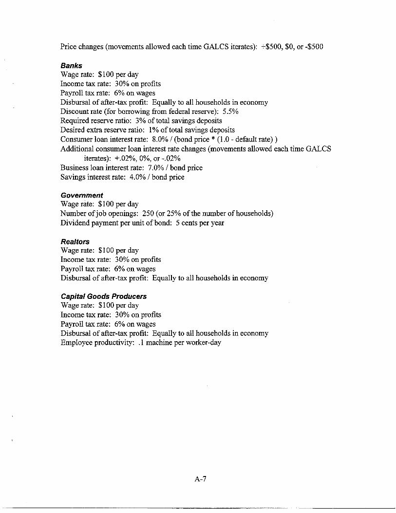
In Appendix B, Graph B 1 records the effects of an expansionary versus a contractionaryfederal reserve policy on loan interest rates. Economic theory dictates that given acontractionary policy, bond prices should be lower because the federal reserve is sellingbonds. The lower price in turn implies that bonds have a higher “effective yield” as aninvestment. Hence, the banks will invest more in bonds and less in other investments,such as the giving out of loans. This lowered supply of bank loan money implies that weexpect the loan interest rates to increase. This is in fact exactly what Graph B 1 shows.
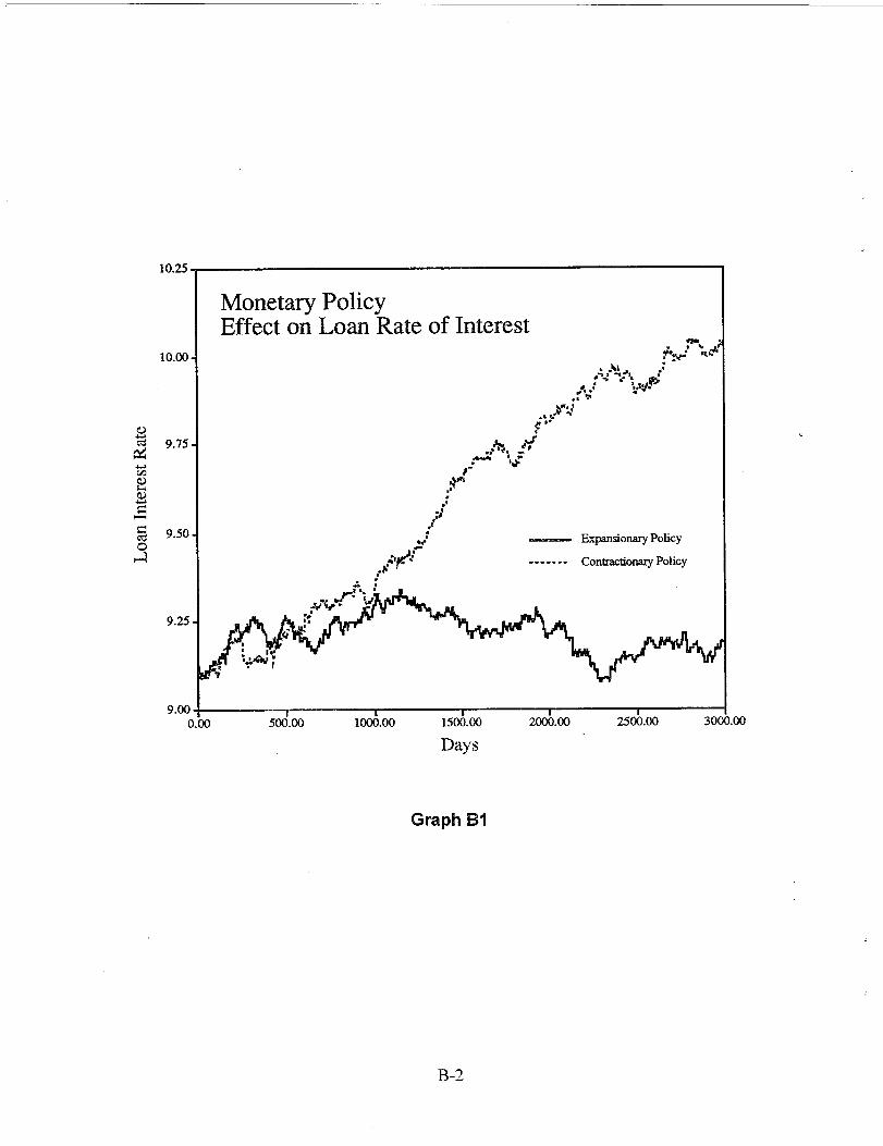
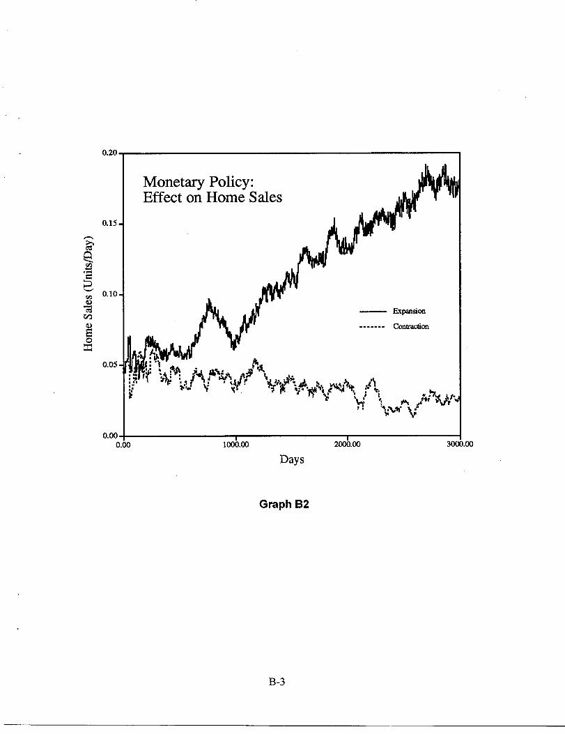
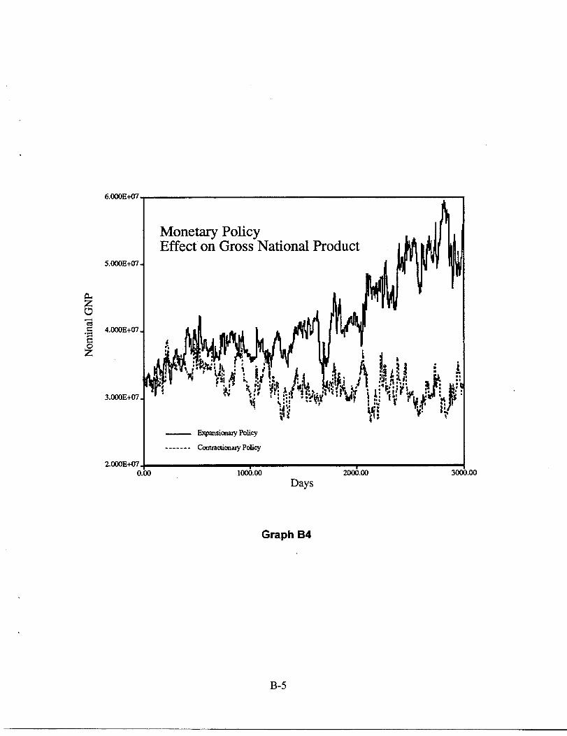
Graphs B2, B3, and B4 illustrate the secondary effects of loan-rate increases. An increasein loan rates means consumers can afford less expensive autos and homes. Alsoconsumers are less likely to purchase a home. Reduced sales imply increased inventory,reduced employment, and reduced income. Graph B2 illustrates these observations.Also, with higher interest rates, firms are less likely to make new investments in capitalmachinery. Hence, productivity, production, and profits suffer. In the Sandia model,lower profits mean lower household incomes and dropping consumer demand. Graph B3illustrates that reduced demand causes prices to drop. This, combined with lowerproduction and consumption gives lower nominal gross national product (GNP), asshown in graph B4.
12
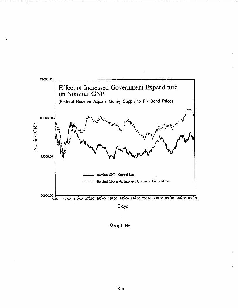
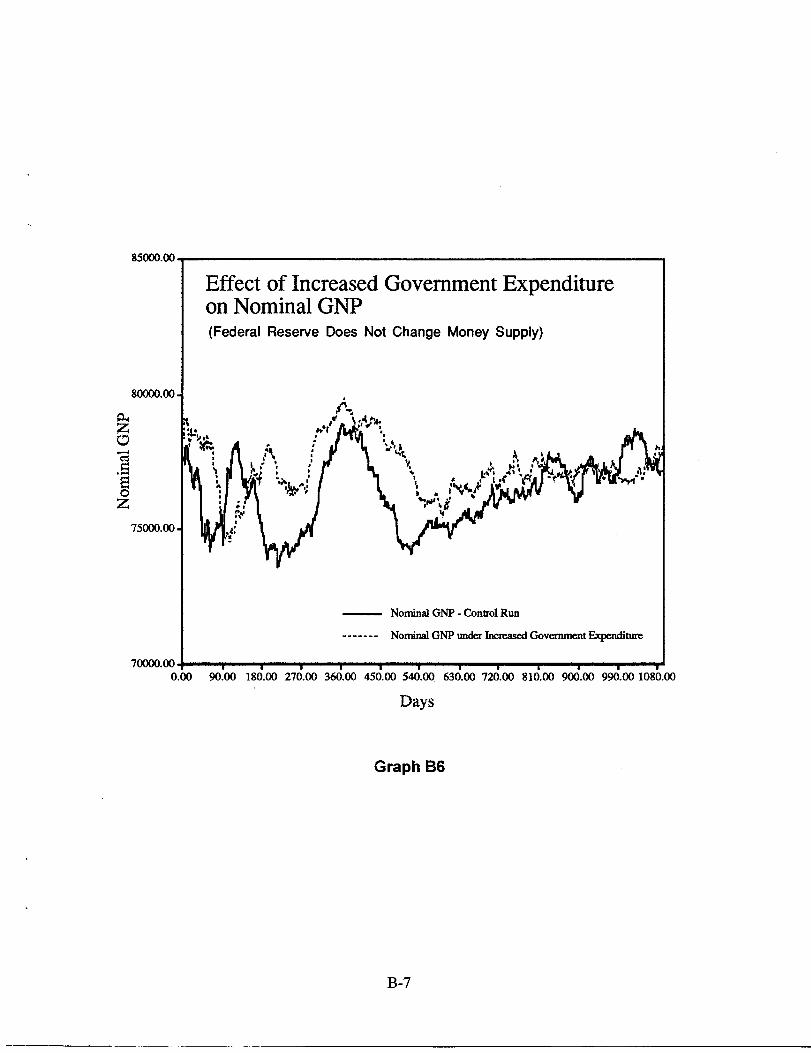
Finally, we successfully reproduced on our model some of Modigliani’s (1972)experiments on the FMP12 model. Specifically, we increased government spending by$1,000 per day for three years and observed the multiplier effects on the economy.
The resultant government expenditure multiplier is not properly defined unless we specifithe monetary policy to be followed by the federal reserve over the period. Hence, Sandiaperformed the experiment under two monetary policy scenarios and noted the differencein run outputs. The first scenario had the federal reserve agent conduct a stabilizingmonetary policy of keeping bond price at $1 (see Federal Reserve); the second scenariohad the federal reserve agent conduct a fixed money supply policy (that is, the agentbought a constant number of bonds each period). Unlike the first scenario, the bond pricein the second scenario was allowed to change.
Graph B5 displays a 10-run average of nominal GNP for the Sandia model in thestabilizing case. The nominal GNP is shown with and without the $1,000/day fiscalexpansion (described immediately above). Graph B6 illustrates the same for a constantmoney supply case. Comparing these two graphs reveals much greater effect on nominalGNP in the stabilizing case than in the fixed money supply case. Modigliani alsoobtained this intuitive result.
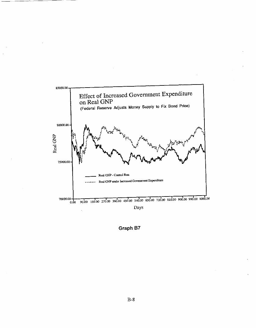
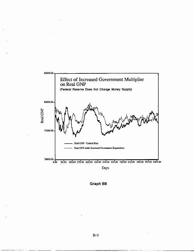
Graphs B7 and B8 show the same effect on real (inflation-corrected) GNP.
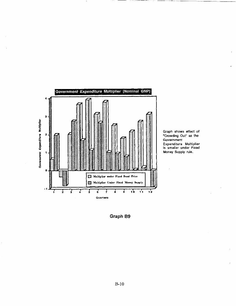
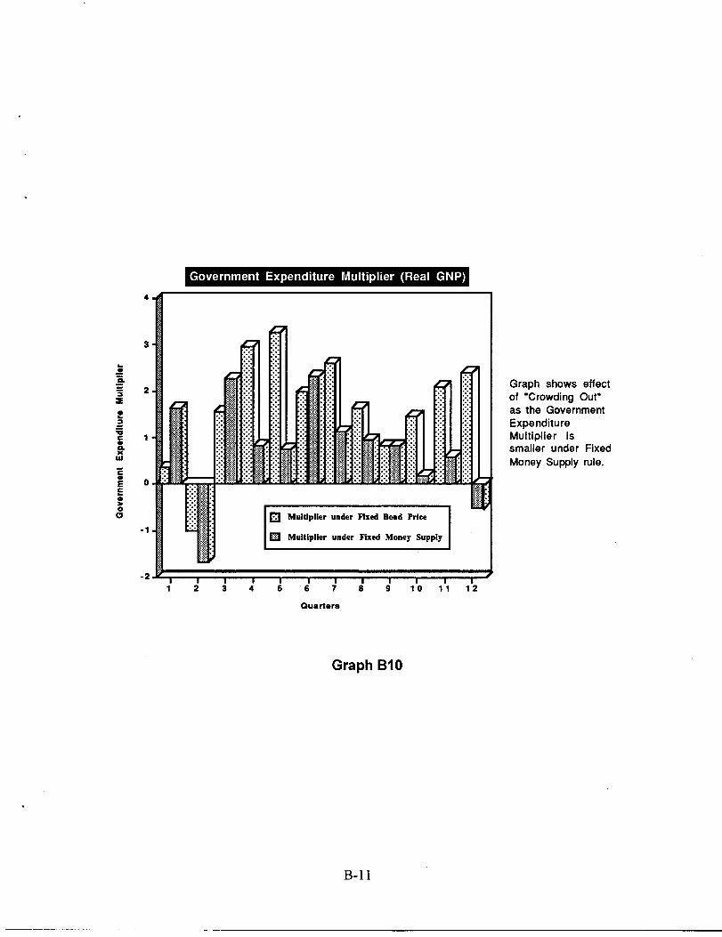
Graphs B9 and B 10 illustrate these effects quantified for government expendituremultipliers. These quantifications almost duplicate Modigliani’s findings. The multiplieron nominal GNP reaches a value of close to 4 by the fiflh quarter under stabilization.However, the multiplier is much smaller under the fixed money supply rule. In the lattercase, the increase in bond interest rate reduces increased income. This “crowding out” isquite pronounced in both the nominal GNP and real GNP numbers.
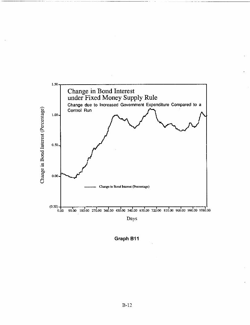
A change in government spending affects bond and loan interest rates. Increasedgovernment expenditure implies more deficit and, therefore, an increase in bond supply.In the fixed-money-supply case, this increased deficit and bond supply should cause anincrease in the interest rate for bonds. Graph B 11 demonstrates this.
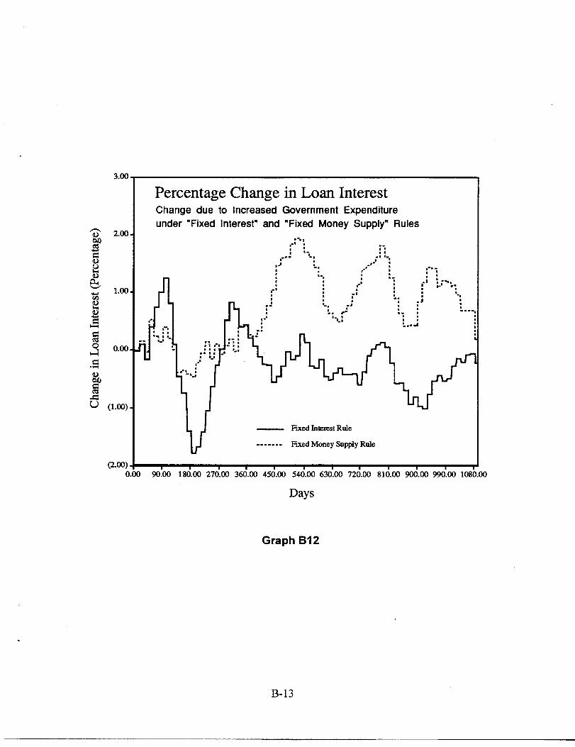
Regarding loan interest, since the banking industry is highly oligopolistic, all banks lookat a common signal (the bond price) to determine rates. As bond prices drop, bank loaninterest rates rise. Hence, in the fixed-money-supply case, the fiscal expansion shouldlead to an increase in loan interest rates. However, in the stabilization case when thebond price is constant, loan interest rates should stay relatively constant. Graph B 12supports this theory.
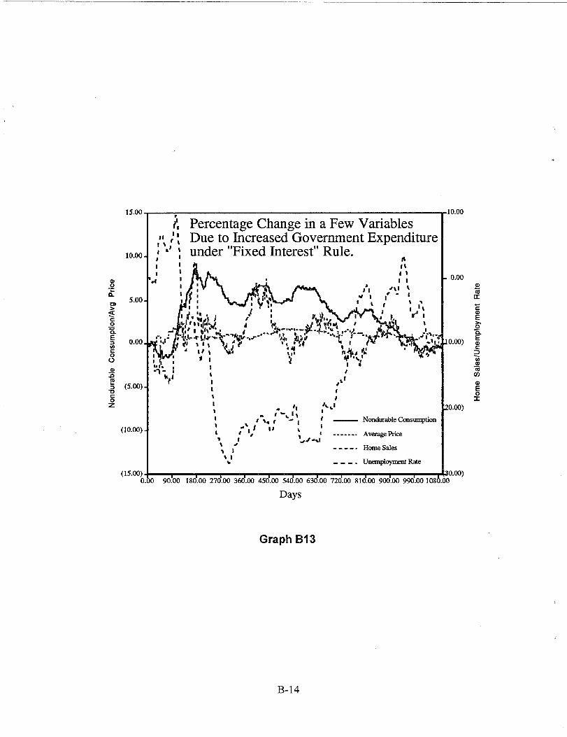
Finally, some fbrther results are presented for the stabilization case. Graph B 13 showsthe effect of increased government expenditure on nondurable-goods consumption,
12FMP stands for Federal Reserve – MIT – University of Pennsylvania.
13
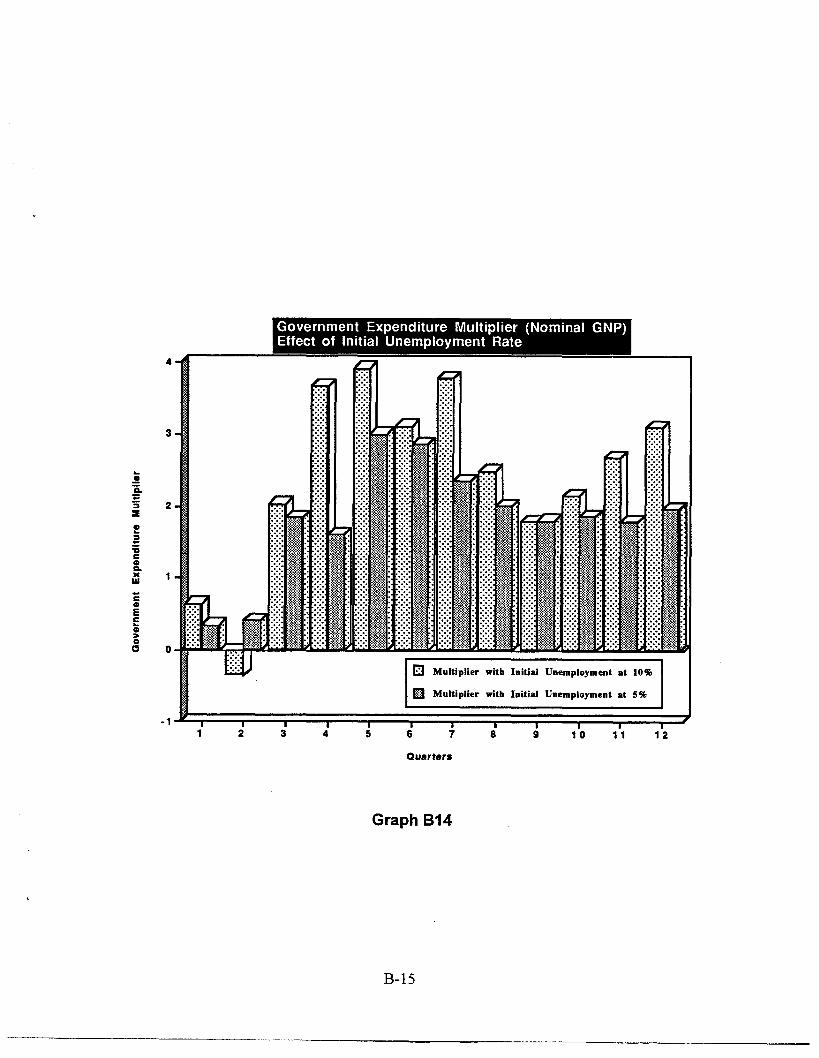
average price level, home sales, and the unemployment rate. The effect of stabilizationon the unemployment rate is substantial. This study inquired if the initial unemploymentrate affected the multiplier for nominal GNP. Graph B 14 (the result of that inquiry)indicates that the multiplier is higher if the initial unemployment level is set at 10°/0thanif the initial unemployment rate is set at 5°/0. Again, this finding duplicates a Modiglianitest result from the FMP model.
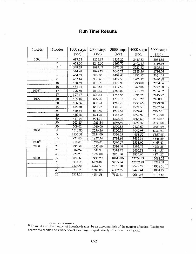
Run Times and Agent Location
This study also examined how processing time for an Aspen run varies as a fimction ofthe number of Paragon computer nodes. In general, the run time can be broken into (a)time needed to send messages between agents on the same node, (b) time needed to sendmessages between agents on different nodes, and (c) time needed for agents to carry outall other tasks. In general, (a) is insignificant. Also, as the number of nodes increases(but the number of agents n stays constant), (b) increases because there are more nodesand more cross-nodal packets (see Mechanics of the Model) to be sent during each stage.At the same time, (c) decreases because of the increased ability to compute in parallel. Infact, if x represents the number of nodes, the run time @er stage) can be estimated as
~x + @x where ~ and y are constants associated with (b) and (c) respectively, withp << ’y.1~
The function ~x + p/x is convex with a unique minimum. Given a certain agent set,there should bean optimum number of nodes on which to run a problem. The Sandiastudy verified this. This study made a series of runs, all using 1,000 households and thedefault values listed in Appendix A. Only the number of nodes were varied, with tworuns for each different node number. These results (see Appendix C) indicate that (a) runtimes are remarkably consistent from run to run if the node number is constant, (b) runtime is linear in the number of time steps, and (c) the optimal number of nodes isapproximately 17. These same runs were made using 2,000 households and then 5,000households. The optimal number of nodes rose to the 20 to 25 range.
Agent distribution on the nodes was examined when the node number is fixed.Government, federal reserve, and all bank and firm agents might seem appropriatelyplaced on the same node. The remaining nodes might seem best dedicated to householdagents because households do not send messages to one another. This arrangementwould minimize the number of cross-nodal packets (see Mechanics of the Model).
13Here ~ represents (a constant multiplied by) the average time to send a cross-node communication, and yis the time for an agent to perform all activities of a stage. The expression depends on most nodescontaining only household agents, and household agents not sending messages to one another in the currentversion of Aspen. If we were to develop a model in which household agents do send messages to one
another, then the correct expression would be (3x(x-1) + yn/x. This would not change the logic in whatfollows.
14

However, in that case the node with nonhousehold agents would take far longer toprocess all members than would any other node. In Aspen all nodes must finishprocessing all members before the run can proceed to a new stage. Hence, the modelwould run more slowly; time would be wasted as the household nodes waited for thenonhousehold node to finish.
In the current version of Aspen, the government and federal reserve agents are placed onthe first node; the firms and banks are distributed over the second, third, and fourthnodes; and the households are distributed equally over all the nodes. This more balancedsetup may alleviate the above problem, but at the expense of increasing the number ofcross-nodal packets. In conclusion, fhrther study is required to determine a method forefficient agent placement.
GALCS: Further Discussion
The Firms discussion did not fully explain how the quantitative changes in the probabilityvectors p = (pD,pI, pc) were computed. This study tried many variations. In all cases,each state was assigned a three-dimensional strength vector, initialized at (100, 100, 100).When a firm enters a state and then raises, maintains, or lowers a price, the strengthvector subsequently changes. When normalized, this vector becomes the new p. Sandiaexperiments used different procedures to change the strength vector.
One such procedure was to raise or lower the component of the strength vector associatedwith the corresponding action by 10. Whether the component was raised or lowereddepended on whether the action was successful. In other words, if the strength is at (100,100, 100) and the price is increased, then the new strength vector will be (100, 90, 100) ifprofit level drops or (100, 110, 100) if the profit increases.
A problem with this method is that, although strengths of (10, 20, 30) and (20, 40, 60)will compute to the same p, the probability vectors that occur after the next evaluation aredifferent. A second problem is that the GALCS can become overtrained if the economychanges suddenly after a period of stability. In this case, the probabilities for certainstrategies might approach zero, making reaction to the new environment impossible for afirm.
In response to differing probability vectors, this study tried increasing or decreasing thestrengths of the other components to maintain the sum of the strength components at 300.In the example above where the profit level drops, the new strength vector was (105,90,105) instead of (100, 90, 100).
In response to overtrained GALCS resulting ftom a period of economic stability, thisstudy restricted how high or low a strength component could go.
15
Another issue was whether to consider first- or second-order effects to decide if a pricechange increased the profit. In certain scenarios (notably the expansionary orcontractionary cases described in Economic Results), profits increased (or decreased)regardless of pricing strategy. Hence any strategy tried would be positively (negatively)reinforced, leading to somewhat unrealistic results. This led us to experiment with usinga second-order condition on profits to determine success; that is a certain pricing strategywould get reinforced if and only if the amount of profit-increase increased.Unfortunately, determining the second-order effects requires profit analysis over a periodof time; this profit analysis uses observations that may have been taken under a differentpricing strategy.
Finally, we tried linking the magnitude of the strength-vector changes to the magnitude ofthe profit changes. This avoided the problems described in the previous paragraph. The
best results (vectors p agreeing with our intuition about what firms should do in variousstates) were obtained using this linkage.
GALCS and Prices: Final Observation
Consider a two-food firm economy in which the firms behave as those described in theFirms section. The first food firm’s expected profit can be estimated as
III = (j] - C) * @l-q/@l-q+ pz-q) ) * a,
wherepl = price first firm chargespz = price second firm chargesC = wage/worker productivity14q = demand exponent (see Household (Individuals).a = constant marketwide household demand for food (units).
Similarly, 112can be expressed as the expected profit for the second firm. A two-persongame may be described where the players are firms and the strategies are the prices thefirms charge. Under steady-state demand conditions, a unique equilibrium of the gameoccurs when pl = p2 = qC/(q-2). In fact, when Sandia ran a prototype version of Aspen(described by Pryor-Basu-Quint [1996]) with two food firms, prices hovered near thesevalues. Here, the genetic algorithms lead to prices dictated by theory.
14Worker productivity is defined as the quantity of goods produced per worker day. In the model in the
Firms section (first paragraph) with a=b= 1, workerproductiviz’yrefers to the quantity cK. Regarding theprototype model (where firms cannot buy capital), the quantity is a given constant.
16
Conclusion
At its present level of development, Aspen is not yet ready to make quantitative forecasts.We acknowledge that certain sectors of the model need to be added or improved and thatmany parameters need to be estimated accurately. However, the economic results seem tovalidate the approach described here. Indeed, simulation models such as Aspen areexpected eventually to complement the existing macroeconometric and CGE models,perhaps with superior analytic and forecasting capabilities.
17
References
Bergmann, B. and R. Bennett, A Microsimulated Transactions Model of the United StatesEconomy, Baltimore: The Johns Hopkins University Press, 1986.
Modigliani, F., “The Channels of Monetary Policy in the FMP Econometric Model of theUSA”, in Modeling the Economy, Heineman Educational Books: London, 1976.
Orcutt, G., S. Caldwell, and R. Wertheimer, Policy Exploration through MicroanalyticSimulation, Washington, DC: The Urban Institute, 1976.
Pryor, R.J., N. Basu, and T. Quint, “Development of Aspen: A Microanalytic SimulationModel of the US Economy”, Sandia Report #SAND96-0434, Sandia NationalLaboratories, Albuquerque, NM, February 1996.
Varian, H., Macroeconomic Analysis, New York: W.W. Norton and Co, 1978.
18

Intentionally Left Blank
APPENDIX A
Initializing Values and Creating Parameters
Initializing Values and Creating Parameters
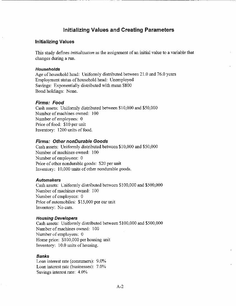
Initializing Values
This study defines initialization as the assignment of an initial value to a variable thatchanges during a run.
HouseholdsAge of household head: Uniformly distributed between 21.0 and 76.0 yearsEmployment status of household head: UnemployedSavings: Exponentially distributed with mean $800Bond holdings: None.
Firms: FoodCash assets: Uniformly distributed between $10,000 and $50,000Number of machines owned: 100Number of employees: OPrice of food: $10 per unitInventory: 1200 units of food.
Firms: Other nondurable GoodsCash assets: Uniformly distributed between $10,000 and $50,000Number of machines owned: 100Number of employees: OPrice of other nondurable goods: $20 per unitInventory: 10,000 units of other nondurable goods.
AutomakersCash assets: Uniformly distributed between $100,000 and $500,000Number of machines owned: 100Number of employees: OPrice of automobiles: $15,000 per car unitInventory: No cars.
Housing DevelopersCash assets: Uniformly distributed between $100,000 and $500,000Number of machines owned: 100Number of employees: OHome price: $100,000 per housing unitInventory: 10.0 units of housing.
BanksLoan interest rate (consumers): 9.0?40Loan interest rate (businesses): 7.0%Savings interest rate: 4.0%
A-2
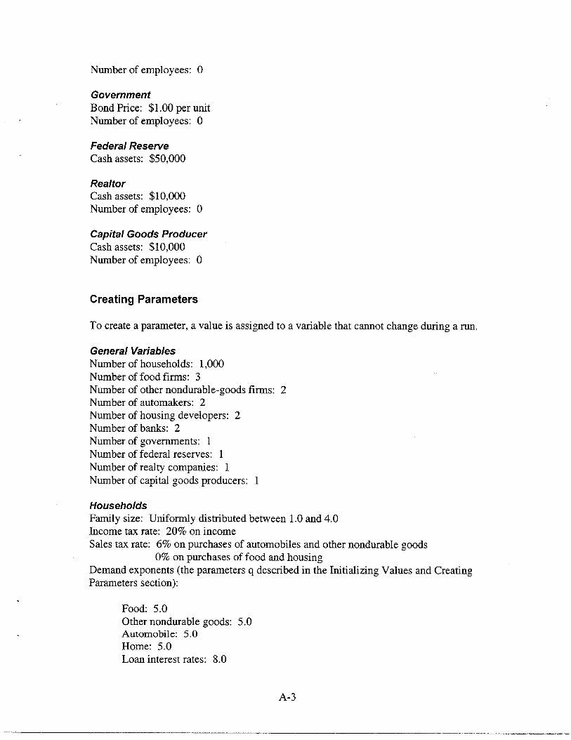
Number of employees: O
GovernmentBond Price: $1.00 per unitNumber of employees: O
Federal ReserveCash assets: $50,000
RealtorCash assets: $10,000Number of employees: O
Capital Goods ProducerCash assets: $10,000Number of employees: O
Creating Parameters
To create a parameter, a value is assigned to a variable that cannot change during a run.
General VariablesNumber of households: 1,000Number of food firms: 3Number of other nondurable-goods firms: 2Number of automakers: 2Number of housing developers: 2Number of banks: 2Number of governments: 1Number of federal reserves: 1Number of realty companies: 1Number of capital goods producers: 1
HouseholdsFamily size: Uniformly distributed between 1.0 and 4.0Income tax rate: 2070 on incomeSales tax rate: 6% on purchases of automobiles and other nondurable goods
O% on purchases of food and housingDemand exponents (the parameters q described in the Initializing Values and CreatingParameters section):
Food: 5.0Other nondurable goods: 5.0Automobile: 5.0Home: 5.0Loan interest rates: 8.0
A-3
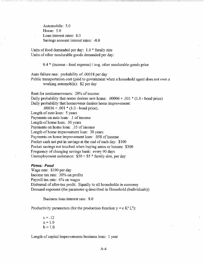
Automobile: 5.0Home: 5.0Loan interest rates: 8.0Savings account interest rates: -8.0
Units of food demanded per day: 1.0 * family sizeUnits of other nondurable goods demanded per day:
0.4 * (income - food expense)/ avg. other nondurable-goods price
Auto failure rate: probability of .00018 per dayPublic transportation cost @aid to government when a household agent does not own a
working automobile): $2 per day
Rent for nonhomeowners: 20’% of incomeDaily probability that renter desires new home: .00006 + .001 * (1.0 - bond price)Daily probability that homeowner desires home improvement:
.00036 + .001 * (1.0 - bond price),Length of auto loan: 5 yearsPayments on auto loan: .1 of incomeLength of home loan: 30 yearsPayments on home loan: .35 of incomeLength of home improvement loan: 30 yearsPayments on home improvement loan: .058 of incomePocket cash not put in savings at the end of each day: $100Pocket savings not touched when buying autos or houses: $300Frequency of changing savings bank: every 90 daysUnemployment assistance: $50 +$5 * family size, per day
Firms; FoodWage rate: $100 per dayIncome tax rate: 30% on profitsPayroll tax rate: 6’XOon wagesDisbursal of after-tax profit: Equally to all households in economyDemand exponent (the parameter q described in Household (Individuals)):
Business loan interest rate: 8.0
Productivity parameters (for the production function y = c K’ Lb):
C= .12a=l.Ob=l.O
Length of capital improvements business loan: 1 year
A-4
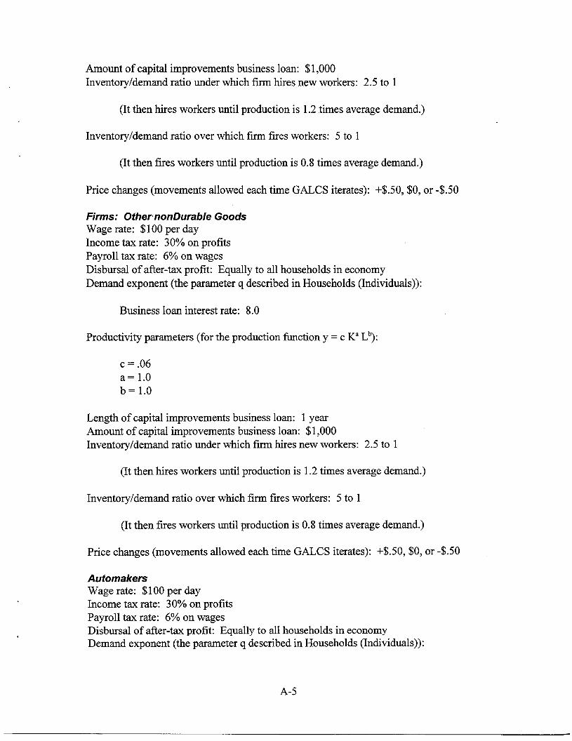
Amount of capital improvements business loan: $1,000Inventory/demand ratio under which firm hires new workers: 2.5 to 1
(It then hires workers until production is 1.2 times average demand.)
Inventory/demand ratio over which firm fires workers: 5 to 1
(It then fires workers until production is 0.8 times average demand.)
Price changes (movements allowed each time GALCS iterates): +$.50, $0, or -$.50
Firms: OfhernonDwab/e GoodsWage rate: $100 per dayIncome tax rate: 30% on profitsPayroll tax rate: 6% on wagesDisbursal of after-tax profit: Equally to all households in economyDemand exponent (the parameter q described in Households (Individuals)):
Business loan interest rate: 8.0
Productivity parameters (for the production function y = c K’ Lb):
C= .06
a= 1.0b= 1.0
Length of capital improvements business loan: 1 yearAmount of capital improvements business loan: $1,000Inventory/demand ratio under which firm hires new workers: 2.5 to 1
(It then hires workers until production is 1.2 times average demand.)
Inventory/demand ratio over which firm fires workers: 5 to 1
(It then fires workers until production is 0.8 times average demand.)
Price changes (movements allowed each time GALCS iterates): +$.50, $0, or -$.50
AutomakersWage rate: $100 per dayIncome tax rate: 30% on profitsPayroll tax rate: 6% on wagesDisbursal of after-tax profit: Equally to all households in economyDemand exponent (the parameter q described in Households (Individuals)):
A-5
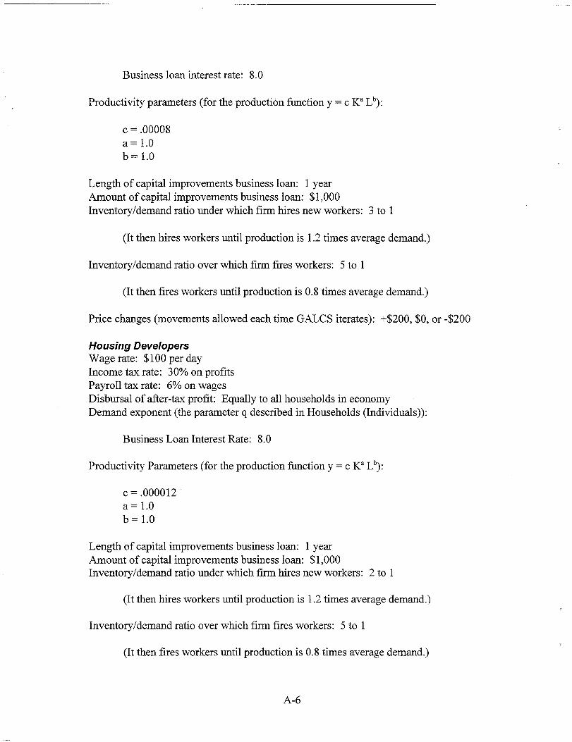
Business loan interest rate: 8.0
Productivity parameters (for the production fimction y = c K’ Lb):
C= .00008a= 1.0b=l.O
Length of capital improvements business loan: 1 yearAmount of capital improvements business loan: $1,000Inventory/demand ratio under which firm hires new workers: 3 to 1
(It then hires workers until production is 1.2 times average demand.)
Inventory/demand ratio over which firm fires workers: 5 to 1
(It then fires workers until production is 0.8 times average demand.)
Price changes (movements allowed each time GALCS iterates): +$200, $0, or -$200
Housing DevelopersWage rate: $100 per dayIncome tax rate: 30% on profitsPayroll tax rate: 6% on wagesDisbursal of after-tax profit: Equally to all households in economyDemand exponent (the parameter q described in Households (Individuals)):
Business Loan Interest Rate: 8.0
Productivity Parameters (for the production fi.mction y = c Ka Lb):
c = ,000012a= 1.0b=l.O
Length of capital improvements business loan: 1 yearAmount of capital improvements business loan: $1,000Inventory/demand ratio under which firm hires new workers: 2 to 1
(It then hires workers until production is 1.2 times average demand.)
Inventory/demand ratio over which firm fires workers: 5 to 1
(It then fires workers until production is 0.8 times average demand.)
A-6
Price changes (movements allowed each time GALCS iterates): +$500, $0, or -$500
BanksWage rate: $100 per dayIncome tax rate: 30% on profitsPayroll tax rate: 6’%on wagesDisbursal of after-tax profit: Equally to all households in economyDiscount rate (for borrowing from federal reserve): 5.5%Required reserve ratio: 3?40of total savings depositsDesired extra reserve ratio: 1% of total savings depositsConsumer loan interest rate: 8.0% / (bond price* (1.0 - default rate))Additional consumer loan interest rate changes (movements allowed each time GALCS
iterates): +.02°/0, 0°/0,or -.020/0Business loan interest rate: 7.0%/ bond priceSavings interest rate: 4.0% / bond price
GovernmentWage rate: $100 per dayNumber of job openings: 250 (or 25% of the number of households)Dividend payment per unit of bond: 5 cents per year
RealtorsWage rate: $100 per dayIncome tax rate: 30% on profitsPayroll tax rate: 6% on wagesDisbursal of after-tax profit: Equally to all households in economy
Capital Goods ProducersWage rate: $100 per dayIncome tax rate: 30% on profitsPayroll tax rate: 6% on wagesDisbursal of after-tax profit: Equally to all households in economyEmployee productivity: .1 machine per worker-day
A-7

Intentionally Left Blank

APPENDIX B
Graphs Illustrating Study Results
lU.L2
10.00
9.75
9.50
9.25
9.04I
Monetary PolicyEffect on Loan ‘Rate of Interest
— ExpansionaryPolicy
.#’’#”s: ------- ContfactiormyPolicy
.
I I I I I9 500.00 1000.OO 1500.00 2000.00 2s00.00 31
Dal)%
‘
K)(3
B-2
0.20
0.15
0,10
0.05
0.00(
Monetary Policy:Effect on Home Sales
— Expansion
------- contraction
I I)
11000.00 2000.00 30CQ.00
Days
B-3
12.00
1.00
0.00
9.00
8.00[
Monetary PolicyEffect on Non-durable Prices
f
-------
Expansionaly Policy
ContractionaryPolicy
) looixil 2006.OQ 3CH
Days
Loo
Graph B3
B-4
6.M10E+07
5.000E+07
4.000E+07
3.000E+07
2.000E+07(
Monetary PolicyEffect on Gross National
— ExpansionaryPolicy
------- contnX?imaryPolicy
} 1006.00 2006.00 3(
Days
85000.00
80000.00
75000.00
70000.00(
Effect of Increased Government Expenditureon Nominal GNP(Federal Reserve Adjusts Money Supply to Fix Bond Price)
Jr-:an
Nominal GNP - Control Run
------- Nominal GNP under Incmsed Government Expenditure
I 1 1 I n 1 1 # I 1 1 I
) 90.00 180.00 270.00 360.00 450.00 540.00 630.00 720.00 810.00 900.00 990.00 1080.00
Days
Graph i35
85000.00
75000.00
70000.000
Effect of Increased Government Expenditureon Nominal GNP(Federal Reserve Does Not Change Money Supply)
,6-,
— Nominal GNP - Contiol Run
------- NominalGNP under Inmased GovernmentExpenditure
) 90:00 180.CO 270.CQ 360.00 450.00546.00 630.00 72&10 810.00 906.00 996.001080.00
Days
Graph B6
85000.00 1
Effect of Increased Government Expen&mreon Real GNP(Federal Reserve Adjusts Money Supply to Fix Bond Price)
_ RealGNP- Coowl Run
. . . . . . . RealGNPunderIncrea=dGovernmentExpenditure
II 1 I 1’
7mw”0~.~o ~o!oo 180.00 270.@ 360+00 450.00 5L$(MxJ630.00 720.00 81O.OO900.WI 990.00 108O.OOI I t 1 1 1 I I
85000.00
80000.00
%
$+
3
75000.OC
Effect of Increased Government Multiplieron Real GNP(Federal Reserve Does Not Change Money Supply)
_ RealGNP- ConmlRun
------ RealGNPun&rIncreasedGovuxunmtExpuldiwre
70000.00 8 , m 8 1 1 1 10.00 90.00 180.00 270.00 360.00 450.00 540.00 630.00 720.00 81&10 90&CMl990.00 1(
I
Days
Graph B8
Qo
B-9
3
2
1
0
.1
❑ Multiplier under Fixed Bond Price
❑ Multiplier Under Fixed Money Supply
i~34 56789101-1 12
Quarters
Graph shows effect of“Crowding Out” as theGovernmentExpenditure Multiplieris smaller under FixedMoney Supply rule.
Graph B9
B-10
4
3
2
1
0
-1
-2
a
LY,:,:.:.~;: L 4::::::,
1234567 89101112
Quartera
Graph BIO
Graph shows effectof “Crowding Out”as the GovernmentExpenditureMultiplier issmaller underMoney Supply
Fixedrule.
B-1 1
1.50
1.00
0.50
0.00
(0.50)(
Change in Bond Interestunder Fixed Money Supply RuleChange due to Increased Government Expenditure Compared to aControl Run
— Change in Bond Interest (Fwcentage)
I 1 I i 1 I I I I I I f) 90.00 180.00 270.00 360.00 450.00 540.00 630.00 720.00 810.00 900.00 99Q.00 1080
Days
)0
Graph BI 1
B-12
3.00
2.00
1.00
0.00
u)en=
:(J (1.00)
(2.00)c
Percentage Change in Loan InterestChange due to Increased Government Expenditure
under “Fixed Interest” and “Fixed Money Supply” Rules
.-.,,.! ,* :- :;
.. : “-,, .: :.’0*J ‘-, .*-* :* ... , a--:
!,.,-.i●*::..-,.s ,
\
:. ..::.-.
-.4’
— Fixed Interest Rule
------- Fixed Money Supply Rule
I 90:00 180.00 27000 366.00 450.00 540.00 6WJ30 720.00 810.00 906.00990.00 1080.00
Days
B-13
15.00
10.00
5.00
0.00
(5.00)
(10.00)
(15.00)(
/, Percentage Change in a Few VariablesJI t’: Due to Increased Government Expenditure‘‘’ ; under “Fixed Interest” Rule.,8I I A S1 IL
I Ikt
I . . . . . . .4/.%1
-----
----
Nondurable Consumption
Avaage Rice
Home Sak
Unemploymmt Rate
90:00 180’.00270’.00360’.00 450’.00540’.00630’.00 720’.00 810kKl 900’.00990’.00 108/
Days
10.00
0.00)
0.00)
0.00))
Graph B13
B-14
-
(7I...............
tw ❑ Multiplier with Initial Unemployment at 10%
❑ Multiplier with Initial Unemp@ment at 5%
-1 t I I I t 2
1I I I I
2 3 4 5I t
6 7 8I
9 10 11 12
Quartara
Graph B14
B-15

Intentionally Left Blank
.
APPENDIX C
Run Time Results
Run Time Results
# holds # nodes 1000 steps 2000 steps 3000 steps 4000 steps 5000 steps(see) (see) (see) (see) (see)
1000 4 617.58 1224.17 1835.22 2445.53 3054.854 628.30 1244.60 1865.79 2492.15 3116.16
5 549.29 1099.47 1672.59 2223.52 2805.68
5 544.90 1098.17 1646.21 2188.56 2736.76
8 464.69 928.05 1404.40 1881.52 2361.05
8 I 467.14 938.46 1427.55 1905.17” 2440.88
10 430.59 876.96 1329.98 1790.00 2254.86
10 434.44 870.65 1317.52 1769.06 2227.38
1003’5 17 396.60 817.63 1264.07 1718.79 2154.82
17 397.47 820.41 1255.88 1695.75 2145.72
1000 20 405.16 829.70 1270.36 1717.29
25 415.30 851.72 I 1306.:
2160.2120 406.36 830.74 I 1268.25 1737.66 2189.30
lo 1771.53 2267.5425 410.34 841.56 1279.67 1724.48 2187.0740 436.48 894.76 1365.22 1857.92 2353.9840 437.14 904.21 1378.06 1866.60 2372.07
[028.54 1556.59 2092.47 2637.081.60 2681.59
2000 4 1310.80 2556.26 3800.58 5042.98 6283.53
10 3639.36 4546.59
50 503.25 150 509.02 1040.00 1570.8S ‘]-
5 1155.51 2254.00 3356.05 4J158~ 5557.4510 921.03 1827.54 2734.8
199815 18 810.01 1676.41 2590.07 _3531.00 / 4468:471
40 928.27 1879.80 2851.90 [ 3854.645000 4 3859.60 7
2000 20 795.58 1652.60 1 2516.40 3399.79 4286.2525 804.24 1648.74 2514.72 I 3405.83 4314.55
4874.27
7135.29 10443.86 13766.79 17081.23
5 3314.26 6274.81 9253.54 12252.49 15238.5110 2425.84 4761.53 7131.50 9529.57 11938.3020 2274.90 4588.88 6989.25 9421.44 11884.27, 1 1 I
t25 2312.24 4684.58 7118.41 9611.16 12118.62
— .—15TO run Aspen, the number of households must be an exact multiple of the number of nodes. We do not
believe the addition or subtraction of 2 or 3 agents qualitatively affects our conclusions.
c-2
DISTRIBUTION:
1“ Dr. Guy H. Orcutt 1P.O. BOX989Grantham, NH 03753
1 Jim Shaw 1BergenShaw International1885 Cabana Dr.San Jose, CA 95125-5608
5 Axel Leijonhufvud 1Center for Computable EconomicsDepartment of EconomicsUCLALos Angeles, CA 90095-1477
1 Jim Bullard 1Federal Reserve Bank of St. Louis411 Locust St.
St. Louis, MO 63102
1 Steve L. Gibson 1The Bionomics Institute2173 East Francisco Blvd., Suite CSan Rafael, CA 94901
1 Richard G. Anderson 1
Federal Resefie Bank of St. Louis411 Locust St.St. Louis, MO 63102
1 Peter Yoo 1Federal Reserve Bank of St. Louis411 Locust St.St. Louis, MO 63102
1 Dr. Barbara R. Bergmann 1Economics DepartmentAmerican UniversityWashington, DC 20016
Dan SullivanFederal Reserve Bank of ChicagoDivision of Research230 South LaSalle St.Chicago, IL 60604
Jim MoserFederal Reserve Bank of ChicagoDivision of Research230 South LaSalle St.Chicago, IL 60604
Dr. Lawrence R. KleinUniversity of PennsylvaniaDepartment of EconomicsPhiladelphia, PA 19104
William GorharnThe Urban Institute2100 M Street NWWashington, DC 20037
Craig CoelenThe Urban Institute2100 M Street NWWashington, DC 20037
Christian PetersenThe World Bank1818 H Street NWWashington, DC 20433
Brian McDonaldBureau of Business and Economic ResearchUniversity of New Mexico1920 Lomas NEAlbuquerque, NM 87131-6021
Mike MckeeEconomics DepartmentUniversity of New MexicoAlbuquerque, NM 87131
DISTRIBUTION (Continued):
1 Peter Tinsley 1Federal Reserve BoardDivision of Research and StatisticsWashington, DC 20551
1 Achla Marathe 1Los Alamos National LaboratoryComputing and Communications DivisionCIC-3, Computer Research& Applications,
Stephanie ForrestComputer Science DepartmentUniversity of New MexicoAlbuquerque, NM 87131
Prof. John F. KainEconomics DepartmentHarvard UniversityCambridge, MA 02138
B265LOSAkunos, NM 87545
1 Prof. Michael JerisonSUNY at AlbanyEconomics Department1400 Washington Ave.Albany, NY 12222
1 Prof. Kajal LahiriSUNY at AlbanyEconomics Department1400 Washington Ave.Albany, NY 12222
1 Prof. Hamilton Lankford
SUNY at AlbanyEconomics Department1400 Washington Ave.Albany, NY 12222
1 Dr. Jacques JihaChief Economist, City of New YorkOffice of the ComptrollerMunicipal BuildingNew York, NY 10007
1 Bob MatthewsLegislative Tax Study CommissionAgency Building 4, 14th FloorEmpire State PlazaAlbany, NY 12208
1
1
1
1
1
Prof. Ken BeaucheminEconomics DepartmentUniversity of ColoradoBoulder, CO 80309
Prof. Jeff ZaxEconomics DepartmentUniversity of ColoradoBoulder, CO 80309
Dr. Frederick DunbarNational Economic Research Associates50 Main StreetWhite Plains, NY 10606
Prof. Kenneth ArrowEconomics DepartmentEncina Hall, 4th FloorStanford UniversityStanford, CA 94305
Kurt E. KarlThe WEFA Group401 City AvenueSuite 300Bala Cynwyd, PA 19004
1
1
1
1
1
DISTRIBUTION (Continued):
Dr. Michael R. DonihueAssociate Professor of EconomicsDepartment of EconomicsColby CollegeWaterville, ME 04901
Brian ArthurSanta Fe Institute1399 Hyde Park RoadSanta Fe, NM 87501-8943
Herbert E. Striner4977 Battery LaneBethesda, MD 20814
Mike SimmonsSanta Fe Institute1399 Hyde Park RoadSanta Fe, NM 87501-8943
Prof. Martin ShubikCowles FoundationYale University30 Hillhouse Ave.New Haven, CT 06520
E. H. Barsis1538 Catron Ave. SEAlbuquerque, NM 87123
Daniel BachmanWefa, Inc.800 Baldwin TowerEddystone, PA 19022
111111
6;2020
1111152
MS 01591378143613781378072201511109110911091111081908190129901808990619
V. Dugan, 4500D. Engi, 4504C. Meyers, 4523S. Narath, 45240. Bray, 4524J. Glicken, 6217G. Yonas, 9000R. J. Pryor, 9202T. Quint, 9202N, Basu, 9202R. Allen, 9222E. Hertel, 9231J. McGlaun, 9231N. Singer, 12620Central Technical Files, 8523-2Technical Library, 4414Review & Approval Desk, 12630For DOE/OSTI
Dr. Alice M. RivlinFederal Reserve BoardWashington, DC 20551


