
Graduate Institute of International and Development Studies
International Economics Department
Working Paper Series
Working Paper No. HEIDWP11-2019
Assessment of interest rate and credit transmissionchannels in a context of banking heterogeneity
Sinda Morsi FattoumCentral Bank of Tunisia
July 2019
Chemin Eugene-Rigot 2P.O. Box 136
CH - 1211 Geneva 21Switzerland
c©The Authors. All rights reserved. Working Papers describe research in progress by the author(s) and are published toelicit comments and to further debate. No part of this paper may be reproduced without the permission of the authors.

Assessment of interest rate and credit transmission
channels in a context of banking heterogeneity∗
Sinda Morsi Fattoum †
July 19, 2019
Abstract
This paper analyses monetary transmission mechanism in Tunisia based on two approaches, an
aggregate data analysis by using a Structural Vector Auto regressive (SVAR) model to assess the
impact and the delay of transmission of monetary policy decisions and to identify through which of
the interest rate channel or credit channel, monetary policy stances’ changes could affect the economy;
and, a bank panel data analysis by employing an ARDL model to measure the reaction of the banks’
pricing policy to monetary policy changes. For the SVAR model, a “recursive” system was used to
uncover the dynamic effects of monetary policy shocks. The empirical results show that the interest
rate channel was more effective than the credit channel and that’s from the 8th quarter. For the
ARDL model, the empirical results show that, taken into consideration of the heterogeneity of the
banking system landscape, the banks pricing’s policy are highly dependent upon money market rate’s
changes. In other words, the transmission to lending rates applied to households as well as to firms
is almost complete.
∗The author would like to thank Prof. Cédric Tille and Ms. Elsa Ferreira for supporting this research and Prof. Luca
Gambetti for his many fruitful discussions. The author is grateful to her colleagues for helpful suggestions and comments.
The author would like to thank also The Bilateral Assistance and Capacity Building for Central Banks (BCC program) for
financial support. The views expressed in this paper are those of the author and do not reflect the position of the Central
Bank of Tunisia.†Executive in the Monetary Policy Strategy Department, Study of the transmission channels of monetary policy Division.
email:[email protected]
1
This research project was completed under the BCC programme, which is funded by the Swiss State Secretariat for Economic Affairs (SECO) and implemented by The Graduate Institute, Geneva.
CONTENTS CONTENTS
Contents
1 Introduction 3
2 Tunisian economic landscape 4
2.1 Monetary policy framework and instruments . . . . . . . . . . . . . . . . . . . . . . . . . . 4
2.2 Exchange rate policy framework . . . . . . . . . . . . . . . . . . . . . . . . . . . . . . . . 6
2.3 Banking system framework . . . . . . . . . . . . . . . . . . . . . . . . . . . . . . . . . . . 7
2.4 Macroeconomic development . . . . . . . . . . . . . . . . . . . . . . . . . . . . . . . . . . 14
2.5 The conduct of Monetary Policy . . . . . . . . . . . . . . . . . . . . . . . . . . . . . . . . 16
3 Literature review 18
4 Aggregate data analysis 21
4.1 Methodology, Data . . . . . . . . . . . . . . . . . . . . . . . . . . . . . . . . . . . . . . . . 21
4.2 Results and interpretation . . . . . . . . . . . . . . . . . . . . . . . . . . . . . . . . . . . . 23
4.2.1 Structural Impulse Response Function (SIRFs) . . . . . . . . . . . . . . . . . . . . 24
4.2.2 Relative Contribution of Shocks . . . . . . . . . . . . . . . . . . . . . . . . . . . . . 26
5 Bank Panel data analysis 28
5.1 Methodology . . . . . . . . . . . . . . . . . . . . . . . . . . . . . . . . . . . . . . . . . . . 28
5.2 Variables’ Definitions and Data Sources . . . . . . . . . . . . . . . . . . . . . . . . . . . . 30
5.3 Results and interpretation . . . . . . . . . . . . . . . . . . . . . . . . . . . . . . . . . . . . 30
6 Conclusion 33
7 Appendix 35
8 Bibliography 41
2

1 INTRODUCTION
1 Introduction
The monetary transmission mechanism by which monetary policy actions are transmitted into real econ-
omy has been extensively discussed by economists over years. Understanding how monetary policy can
influence GDP growth and manages inflation and through which channels, increases her effectiveness
and allows the central bank to keep the key macroeconomic variables close to their optimal level. Huge
number of economic papers has addressed the monetary mechanism topic such as Bernanke and Blinder
(1992), Christiano and Eichenbaum (1995), Leeper, and. al. (1996), Christiano, and. al. (1999), Kim,
(1999), Uhlig (2005), and Forni and Gambetti (2010), but unfortunately still no consensus about the
most important mechanism influence the real economy. Taylor (1995) suggests two broad categories to
classify the different theories of the monetary policy’s transmission mechanism: The “money channels”,
which includes the interest rate and exchange rate channels and the “credit channels” which includes the
balance sheet and bank-lending channels.
Understanding the monetary transmission channels is also very important priority for the Central
Bank of Tunisia (CBT) in formulating monetary policy, especially with the macroeconomic imbalances
resulting from a turbulent environment in the aftermath of 2011 Revolution, characterized by a low growth
rates and an inflationary pressures. A better knowledge of monetary transmission channels also helps
to communicate about monetary policy decisions so that the decision-maker can anchor the economic
agents’ expectations.
As the Tunisian economy is known as a credit based economy, where banks play a major role in the
financing of the economy, and the main instrument of the monetary policy’s conducting is the interest
rate, this paper is focused on the study of interest rate and bank-lending channels to assess the important
role of these two monetary transmission channels in dealing especially with GDP growth and inflation.
This paper discusses the conduct of the monetary policy. The approach is based on two levels:
- An aggregate data analysis by employing Structural Vector Auto regressive (SVAR) model to assess
the impact and the delay of a monetary policy decisions and to identify through which of the interest
rate channel or credit channel, monetary policy stances’ changes could effect the economy; For this part,
the empirical results show that Monetary Policy decisions are transmitted to real activity better through
the interest rate channel than the credit channel and that’s from the 8th quarter.
- A bank panel data analysis based on an ARDL and ECM models to measure the reaction of the
banks’ pricing policy to a monetary policy changes. Actually as the banks’ loans constitute the major
part of the financial ressources for most firms and households in Tunisia, assessing the impact of monetary
policy decision on the banks’ behavior is important because it emphasize their heterogeneity character.
It was found that the banks pricing’s policy are highly dependent upon money market rate’s changes. In
other words, the transmission to lending rates applied to households as well as to firms is almost complete.
3
2 TUNISIAN ECONOMIC LANDSCAPE
The rest of the paper is organized as follows. Section 2 presents the stylized facts about monetary
policy, banking sector in Tunisia and the exchange rate policy. Section 3 provides an overview of literature
on the transmission mechanism of monetary policy, for both aggregate and bank level data analysis.
Section 4 and section 5 provide the models structure, data, empirical results and analysis, for respectively
the aggregate and bank level data analysis. Section 6 concludes the paper.
2 Tunisian economic landscape
2.1 Monetary policy framework and instruments
Since the 1990s, the monetary policy pursued by the CBT was discretionary. This orientation is explained
by the commitment of the issuing institution to achieve several objectives at the same time: to support
the economic activity, preserve the financial system’s stability, ensure the viability and sustainability
of the external position and to control the price’s evolution. Thus, each year, the CBT draws up a
monetary program in which a target for the money supply’s growth is announced, taking into account
a macroeconomic scheme previously established by the Government. However, this monetary target
has been dropped because the volatility of money circulation’s velocity and the assessment of inflationary
pressures via the monitoring of monetary developments was rather indicative and did not have a significant
influence on decisions concerning the policy rate.
It was in 2006, when the ambiguity surrounding the CBT’s principal mission was lifted and “preserving
price stability” was assigned as the main objective of the monetary policy. Since then, modernization
work of monetary policy’s analytical framework was performed and a development of many forecasting
models of inflation and output were implemented. Besides, the key rate was consecrated as the main
instrument to counter inflationary pressures.
The law no 2016-35 of April 25th, governing the CBT, and especially its article no 7, defined the main
objective of the CBT which is not only the preservation of price stability but also its contribution to
financial stability to support the economic policy of the State in terms of growth and employment.
Thus, Tunisia is one of the countries that have a monetary policy’s transitional regime. It doesn’t
expressly target the inflation but it has forward-looking policy which looks to anchor the economic agents’
expectations.
To achieve its goal, the CBT uses its forecasts for inflation as an intermediate objective, and the
money market rate (MMR) as an operational target for conducting monetary policy. Thus, according to
its expectations on inflation and on economic growth, the CBT adjusts the level of its policy rate (key
rate) which influences immediately the overnight money market rate (MMR). These latter influences the
structure-by-term of rates, which ultimately affect the financing conditions of all economic actors.
4

2.1 Monetary policy framework and instruments 2 TUNISIAN ECONOMIC LANDSCAPE
To implement the monetary policy, the CBT possesses panoply of instruments. There are operations1 that can be initiated by the CBT (discretionary) and have one of the following forms:
- Main refinancing operations: constitute the main tool for providing liquidity by the CBT. They
play an important role in steering interest rates and to inform about the monetary policy guidance. The
minimum interest rate applied to the main refinancing operations is the key rate of the CBT. This is
set by the Board of Directors of the CBT in a manner consistent with the ultimate objective of price
stability.
- Longer-term refinancing operations: These transactions are intended to provide additional
liquidity for longer maturities than the main refinancing operations.
- Fine-tuning operations: These transactions are carried out on an ad hoc basis to correct the
effect of unforeseen fluctuations in bank liquidity on interest rates. They have a shorter duration than
the main refinancing operations. They may be carried out by means of reverse transactions, currency
swaps for monetary policy purposes or collection of fixed-term deposits.
- Structural operations: These operations aim to manage a situation of deficit or excess liquidity.
They may be carried out through outright purchases or sales of public or private marketable assets
including Islamic sukuk, foreign exchange swaps for monetary policy purposes and collection of fixed-
term deposits or issuance of debt certificates from the CBT.
The main refinancing operations and the longer-term refinancing operations are exclusively carried
out through reverse transactions in the form of secured loans or repurchase agreements. In addition,
there are standing facilities which are operations that can be initiated by banks (non-discretionary). The
banks dispose, since February 2009, of these facilities at the end of the day to meet their need or excess
of liquidity.
- Marginal lending facility: Banks can use the marginal lending facility to obtain from the CBT,
through reverse transactions as a secured loan or reverse repo, liquid assets at twenty-four hours at a
predetermined interest rate using eligible assets as collateral.
- Deposit facility: Banks can use the deposit facility to make 24-hour deposits with the CBT at a
pre-determined interest rate. The CBT provides no guarantee in exchange for these deposits.
Furthermore, there are “reserve requirements 2” which is a form of deposits of banks with the CBT.
This is essentially aimed to stabilize money market rates through the constitution mechanism, and to1In order to protect the balance sheet of the Central Bank of Tunisia against the credit risk, the refinancing operations
are carried out on the basis of an appropriate security. For this purpose and in accordance with a list of criteria definedin Circular No. 2017-02, the Central Bank of Tunisia accepts, as collateral for the refinancing operations, negotiable assetsincluding public and private negotiable debt securities, mobilized through the custodian. Central Tunisia Clearing, andnon-marketable assets materializing bank loans on companies and individuals mobilized directly from the Central Bank viathe central assets eligible for refinancing (CAER).
2The amount of the compulsory reserve is determined by the application to the base constituted by deposits in Tunisiandinar of a fixed rate schedule. The period of constitution of the compulsory reserve for a given month extends from the firstto the last day of the following month. The elements entering into the base of the compulsory reserve are extracted fromthe monthly accounting situation of the month concerned.
5
2.2 Exchange rate policy framework 2 TUNISIAN ECONOMIC LANDSCAPE
create or increase the need for central bank money to enable the CBT to effectively intervene as a liquidity
regulator. So it has an immediate impact on banks’ liquidity and monetary creation via the credit channel.
2.2 Exchange rate policy framework
When the CBT was set up in November 1958, the value of the dinar was defined in relation to a certain
amount of gold; one dinar was equivalent to 2.11588 g of fine gold. With the collapse of Bretton Wood
System, in 1971 after the monetary crisis, a system of anchoring the dinar to the French Franc was set
up. In 1978, the date of the official adoption of the flexible exchange rate regime by the International
Monetary Fund, the dinar has been pegged to a basket of currencies.
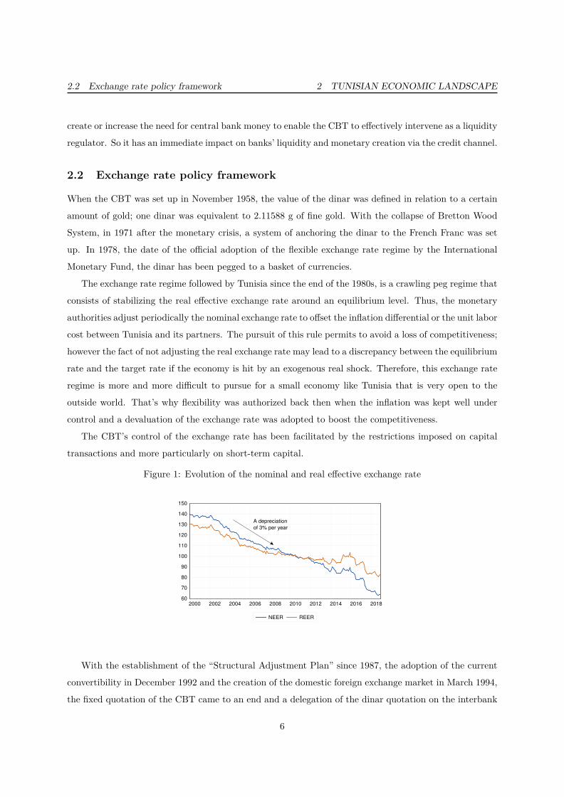
The exchange rate regime followed by Tunisia since the end of the 1980s, is a crawling peg regime that
consists of stabilizing the real effective exchange rate around an equilibrium level. Thus, the monetary
authorities adjust periodically the nominal exchange rate to offset the inflation differential or the unit labor
cost between Tunisia and its partners. The pursuit of this rule permits to avoid a loss of competitiveness;
however the fact of not adjusting the real exchange rate may lead to a discrepancy between the equilibrium
rate and the target rate if the economy is hit by an exogenous real shock. Therefore, this exchange rate
regime is more and more difficult to pursue for a small economy like Tunisia that is very open to the
outside world. That’s why flexibility was authorized back then when the inflation was kept well under
control and a devaluation of the exchange rate was adopted to boost the competitiveness.
The CBT’s control of the exchange rate has been facilitated by the restrictions imposed on capital
transactions and more particularly on short-term capital.
Figure 1: Evolution of the nominal and real effective exchange rate
60
70
80
90
100
110
120
130
140
150
2000 2002 2004 2006 2008 2010 2012 2014 2016 2018
NEER REER
A depreciation
of 3% per year
With the establishment of the “Structural Adjustment Plan” since 1987, the adoption of the current
convertibility in December 1992 and the creation of the domestic foreign exchange market in March 1994,
the fixed quotation of the CBT came to an end and a delegation of the dinar quotation on the interbank
6
2.2 Exchange rate policy framework 2 TUNISIAN ECONOMIC LANDSCAPE
market to authorized intermediaries has taken place. The CBT’s exchange rate policy focused then on
preserving the competitiveness of Tunisia’s economy with its main trading partners and competitors.
In 2011, the CBT began a process of reforms aimed at deepening the foreign exchange market and
developing its capacity to provide the necessary liquidity for economic operators, and to give more weight
to banks as market makers through the promotion of the role of the banks’ Market Makers and the
establishment of a Foreign Exchange Market Maker Agreement.
The reforms undertaken since 2011 have been structured around the four axes:
- Replacement of the dinar’s reference rate published by the CBT by a fixing determined according
to the interbank exchange rates
- Implementation of a "Trade Reporting" system, allowing the CBT to consult and to collect transac-
tions made on the interbank foreign exchange market
- Adoption of a mode of intervention, by the CBT, more active on the exchange market
- Promotion of the role of Market Makers of the banks
In February 2016, a new circular 2016-01 governing the foreign exchange market activity, currency
hedging instruments and interest rate was published to enhance liquidity in the market and boosting
the derivative products’ market. In the same year the IMF classified the Tunisian exchange rate as a
Crawl-like arrangement 3.
Since the beginning of 2010, the political, security and social instability led to a sizable deterioration
of the current account of the balance of payments, which has resulted deterioration in the exchange rate
and had a cost for the Tunisian economy in terms of loss of economic competitiveness. These weighed
heavily on the foreign exchange reserves and thus have contributed significantly to the drop of the number
of days of imports.
In one hand, these depreciations are increasingly squeezing the economic actors, whose have an un-
limited recourse to banks to fund their imports and exports. In the other hand, the continuous growth of
imports outpaces the exports and thus increases the trade deficit and creates a vicious circle. In addition
to all that, the lockout of the phosphate’s production and the recession of the tourist sector for safety
reasons have simply amplified this imbalance. The current account’s deficit represented around 3% of the
current GDP on average between 2000 and 2010, which means before the Revolution. For the year 2017
it reached 10.2%.3Annual report on exchange arrangements and exchange restrictions 2016, International Monetary Fund
7

2.3 Banking system framework 2 TUNISIAN ECONOMIC LANDSCAPE
Figure 2: Evolution of the current account and its main components (in % of Current GDP)
-15
-10
-5
0
5
10
2000 2002 2004 2006 2008 2010 2012 2014 2016
Current account Goods (FOB)Services Factor incomes
Current transfers
Figure 3: Evolution of the foreign exchange reserves and the number of days of imports
4,000
8,000
12,000
16,000
20,000
40
80
120
160
200
2010 2011 2012 2013 2014 2015 2016 2017 2018
Exchange reserves (in TND)
Exchange reserves (in USD)
Number of days of imports (Rhs)
2.3 Banking system framework
The Tunisian economy is known as a credit based economy, where banks play a major role in financing
of 91% 4 of the economy.
The Tunisian banking sector 5 currently involves 23 universal banks: 3 public banks, 5 private banks4By analogy with what was stated by the Managing Director of the BVMT regarding the contribution of the financial
market in the financing of the country’s economy, which currently stands at the level of 9%5Appendix1
8
2.3 Banking system framework 2 TUNISIAN ECONOMIC LANDSCAPE
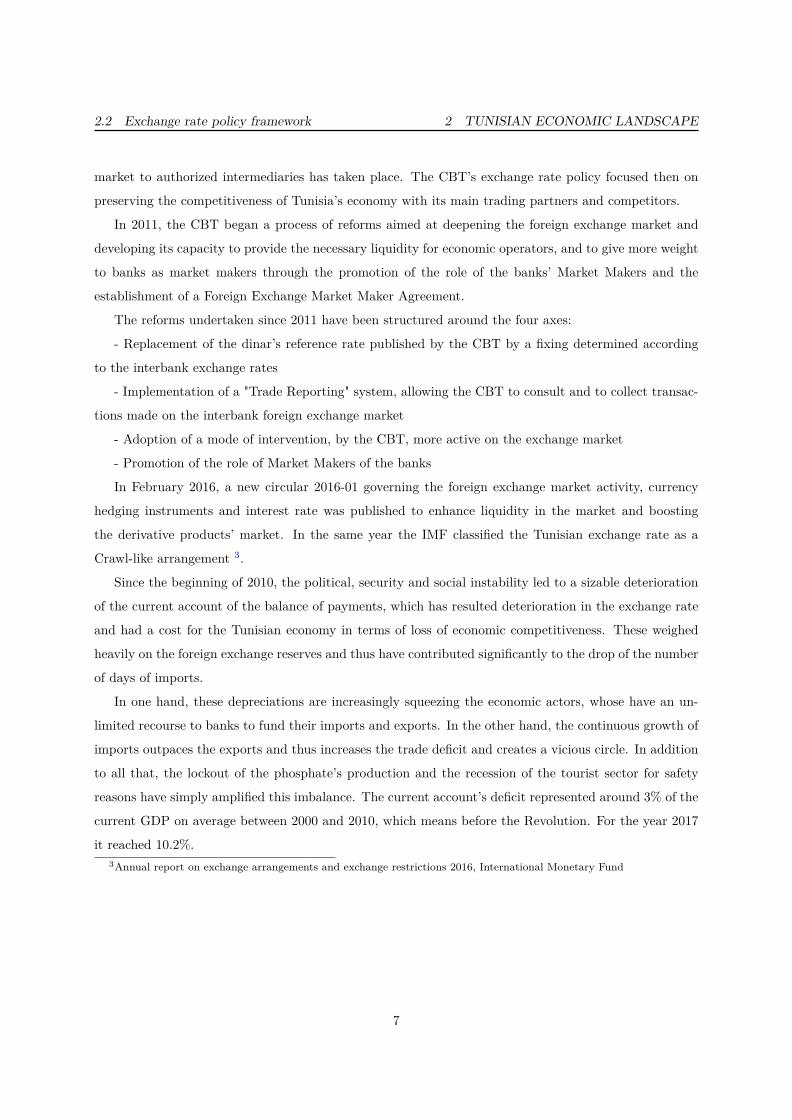
Figure 4: Credits given by banking sector in % of GDP at current prices
45
50
55
60
65
70
75
80
85
2000 2002 2004 2006 2008 2010 2012 2014 2016 2018
80%
with a Tunisian private capital, 2 mixed banks, 10 private banks with a foreign capital, and 3 Islamic
banks. The public ones (3 banks) have the largest market share, almost 41% comparing to the private
banks whose market share is about 59%.
During 2012-2018 periods, the distribution of credits shows that the largest share of credits belongs
to firms comparing to households ones. It represents almost the double of the households’ credits.
The households loans’ portfolio is comprised primarily of loans that maturity is between 3 and 7
years and which implies the housing sitting out credit, with 20% as an average share, flowed by loans
that maturity exceed 7 years and which implies the housing loans with 10% and finally loans that the
maturity is less than 3 years and which implies the consumer credit with only 4%.
The firms loans’ portfolio is comprised primarily of loans that maturity is less than 3 years and which
implies the management loans with 53% as an average, flowed by loans that the maturity is between 3
and 7 years and which are aimed to fund the equipment acquisition and extension project with 10% and
finally loans that the maturity exceed 7 years and which are aimed to fund the investment project with
only 3%.
Whether they are private or public 6, the Tunisian banks’ resources are mainly made of household’s
deposits and borrowing resources which include interbank transactions and refinancing operations with
the CBT.
After the Revolution, the Tunisian banking system knew a large liquidity deficit which led the CBT
to intervene on the money market to provide the necessary liquidity to ensure the financial stability
and to avoid a credit crunch. However, with the rising of inflationary pressures, the CBT has tightened
its monetary policy. But in front of the increase of the liquidity needs of banks, the global volume of
refinancing exceeded 15,000 MTD by the end of December 2018.6After the Revolution, two of the public banks have been recapitalized with the aim of enabling them to respect the
prudential ratios enacted by the CBT, to rebalance the financing of their activities and to return to the profitability as soonas possible.
9

2.3 Banking system framework 2 TUNISIAN ECONOMIC LANDSCAPE
Figure 5: Distribution of credits by agent
Firms Households
66%
34%
Figure 6: Bank loans’ portfolio composition
Firms’ loans Between 3 and 7 years
Firms’ loans Less than 3 years
Firms’ loans More than 7 years
Households’ loans Between 3 and 7 years
Households’ loans Less than 3 years
Households’ loans More than 7 years
53%
10%
3%
4%
20%
10%
10

2.3 Banking system framework 2 TUNISIAN ECONOMIC LANDSCAPE
Figure 7: Evolution of the overall refinancing volume by main operations (in MTD)
-2,000
0
2,000
4,000
6,000
8,000
10,000
12,000
2000
2001
2002
2003
2004
2005
2006
2007
2008
2009
2010
2011
2012
2013
2014
2015
2016
2017
Global Volume of Refinancing 24 h standing deposit facility 24 h standing loan facilityCall for bids Longer-term refinancing operations Open market operationExchange swap
The adoption of a restrictive monetary policy, since 2017, in order to counter inflationary pressures,
the overnight interbank rate reaches 7.24%, by the end of 2018. Hence, a deceleration of credits to the
economy was recorded since the first quarter of the year 2018 and continued till now. This evolution is
explained principally by the slowing down of households’ loans, both the housing and consumer loans,
and to a lesser degree, the firms’ loans.
Moreover, since the banking system is characterized by the indexation of banks’ rates on the MMR 7 ,
an almost automatic transmission of monetary policy to the borrowers’ actual financial costs is therefore
recorded. That allows the CBT to directly influence the "disposable income after interest charges" of
firms and households. It can reduce them, in case of decline of the activity, or increase them when the
activity accelerates.
The graph 8 and 9 shows that the rates applied to households and firms’ loans have followed the money
market trend. This practice preserves the banking system from the interest rate risk that has proved
disastrous in a number of circumstances (eg, US savings banks in the early 1980s and the US banking
system in 2007). The counterpart of banking system’s protection is that, by definition, interest rate risk
is bared by depositors and borrowers, while banks are exposed to the credit risk of their borrowers.
The share of NPLs in public banks is more important than the private one. This is mainly explained,
in addition to the difficult economic situation in Tunisia, by the unpaid loans generated by the tourism
sector and the debts owed to ousted regime insufficiently covered by the collaterals. Firms’ NPL 8 has7which means that rate negotiations are systematically quoted as a deviation from MMR8Annual Report Juin-2017, CBT
11

2.3 Banking system framework 2 TUNISIAN ECONOMIC LANDSCAPE
Figure 8: Lending rates’ evolution of different loans to households
3.0
3.5
4.0
4.5
5.0
5.5
6.0
6.5
7.0
7.5
8.0
8.5
9.0
9.5
10.0
10.5
I II III IV I II III IV I II III IV I II III IV I II III IV I II III IV I II III IV
2012 2013 2014 2015 2016 2017 2018
Households’ loans Between 3 and 7 years
Households’ loans Less than 3 years
Households’ loans More than 7 years
MMR
Figure 9: Lending rates’ evolution of different loans to firms
3.0
3.5
4.0
4.5
5.0
5.5
6.0
6.5
7.0
7.5
8.0
8.5
9.0
9.5
10.0
I II III IV I II III IV I II III IV I II III IV I II III IV I II III IV I II III IV
2012 2013 2014 2015 2016 2017 2018
Firms’ loans Between 3 and 7 years
Firms’ loans More than 7 years
Firms’ loans Less than 3 years
MMR
regressed by 1.9% in 2017 and it’s composed mainly of hotels and restaurants, automotive trade, repair
12
2.3 Banking system framework 2 TUNISIAN ECONOMIC LANDSCAPE
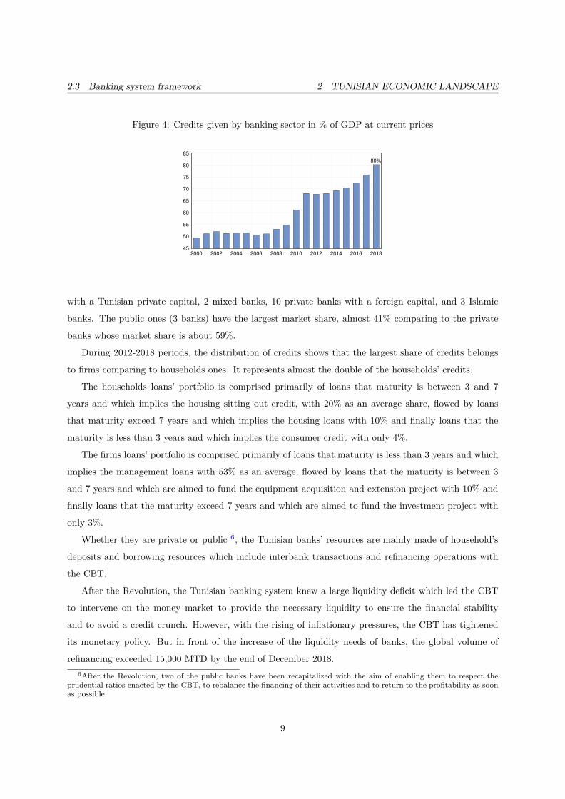
and household goods and finally real estate, renting and business services. The households’ NPL 9 has
decreased by 1.6% due to the decrease of contentious debts’ outstanding.
Figure 10: Evolution of the credits by beneficiary (in %)
0
5
10
15
20
25
30
35
04 05 06 07 08 09 10 11 12 13 14 15 16 17 18
Professionals loans
Households’ loans
Figure 11: Evolution of the credits to the economy and the NPL (in %)
-.05
.00
.05
.10
.15
.20
.25
2004 2006 2008 2010 2012 2014 2016 2018
Credit to the economy NPL
As part of the risk’s management, on one hand, Tunisian banks use the guarantee policy as a major
mean to face up the adverse selection’s risk, at the moment when the credit was granted. This isn’t a
solid solution, since auctions lead to a huge discount of the good’s real value. That explains the fact that
sometimes they ask for a guarantee which represents the double of the credit requested, at the first place.
On the other hand, they adopt a hedging policy that allows covering losses resulting from defaults, as
stipulated by the banking regulations.
Before the revolution, the NPL coverage by provisions was 61.13% on average for private banks and
52.87% for public banks. After the revolution, this rate increased to reach 74% for private banks and9Ditto
13

2.4 Macroeconomic development 2 TUNISIAN ECONOMIC LANDSCAPE
60.88% for public banks. In other words, although public banks have the largest share of nonperforming
loans, they have the lowest coverage ratio. This is what accelerated their recapitalization, after having
undergone a full audit, which pointed out the numerous organizational shortcomings that these banks
had suffered for a long time.
2.4 Macroeconomic development
The Tunisian economic context knew several significant shocks since 2000: The national GDP was nega-
tively impacted, first, by the terrorist attack which tooks place in Djerba, in 2002. Second, the political,
economic and social events that had occurred after January 14, 2011 had also a negative effect on do-
mestic economic activity and its external position. In addition, the slowdown in activity in the Eurozone
countries and political instability, particularly in Libya, had a significant impact on the Tunisian economy.
For this, it is important to describe the framework in which monetary policy is conducted in Tunisia.
Before the Revolution, the GDP growth rate was around 4.3% per year, a rate that did not create
enough jobs or include all regions in the development process. The regional imbalance and the unemploy-
ment of the graduates led to the outbreak of the Revolution. Eight years after the Arab spring, Tunisia
continues to suffer from the instability that has ravaged the economy and has contributed significantly
to the decline in growth.
Figure 12: Evolution of the GDP growth rate (on a year-over-year basis)
-4
-2
0
2
4
6
8
10
2002 2004 2006 2008 2010 2012 2014 2016 2018
GDP
growth rate
around 4,3%
Revolution
Instability and
declination of
GDP growth
rate
Gradual
recovery
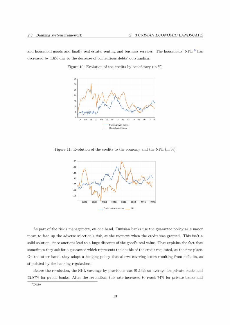
Several endogenous and exogenous factors explain this decrease: The recession in Europe and the
slackening of the foreign demand, in particular that of Europe, contributed to the fall in exports (fallen
to 77% in 2017 while it reached 84% in 2004 10) and the widening of the trade deficit. On the national
level, the slow pace of the democratic transition in addition to political tensions and above all political
assassinations and terrorism depleted the national economy. Besides, the decline in foreign investment,
the collapse of many industrial firms, the deterioration of business climate and the inertia of the tourism10ITC calculations based on UN COMTRADE statistics
14
2.4 Macroeconomic development 2 TUNISIAN ECONOMIC LANDSCAPE
sector, the lack of visibility and confidence in the national economy. All these led to the depreciation
of the local currency, the widening of current account deficit and a reduction of the number of days of
imports.
Figure 13: The degree of synchronization between Tunisia and the European Union countries (in termsof GDP movement)
-6
-4
-2
0
2
4
6
8
2000 2002 2004 2006 2008 2010 2012 2014 2016
National GDP European GDP
Crash of
Autumn 2008
Jasmine
Revolution
Figure 14: Evolution of the Bilateral trade between Tunisia and the European Union countries
55
60
65
70
75
80
85
2000 2002 2004 2006 2008 2010 2012 2014 2016
Import Export
60%
77%
Moreover, after the revolution, the inflationary pressures have occurred and exceeded 7%, by the end
of 2018. It has experienced the highest level, brooked with its usual cycle and persisted over time. This
upward movement is mainly due to: insecurity and supply difficulties in the interior regions; import
inflation mainly caused by the depreciation of the exchange rate (notably the dollar and euro) strongly
affected the imported goods, the energy and food bill and weighed on the state budget, the high cost
of production (due in particular to the rise in wages), which has led to the increase in prices of many
products(wage-price spiral); an exaggerated increase in wages due to a massive recruitment that is not
followed by an increase of labor productivity, a demand shock (especially food) from Libyan refugees
15

2.5 The conduct of Monetary Policy 2 TUNISIAN ECONOMIC LANDSCAPE
which provoked a disequilibrium between supply and demand; the development of counter-tape, parallel
market and the leakage of products, especially of mass consumption, the lack of rigorous economic control,
etc.
Figure 15: Evolution of the Main indicators of core inflation (in %)
1
2
3
4
5
6
7
8
9
00 01 02 03 04 05 06 07 08 09 10 11 12 13 14 15 16 17 18
Core inflation (Excluding regulated prices and frech food)
Core inflation (free of energy and frech food)
Inflation
8.3%
7.5%
Finally but not the least, there was an eruption of liquidity deficit on the interbank market. That
is mainly explained by the decline in activity. This phenomenon has had a significant impact on bank
deposits and current account deficit, which has kept pressure on the market exchange rate and, conse-
quently, liquidity in dinars. However, the examination of the liquidity rate of the economy, measured by
the M311/GDP ratio shows that the money supply has reached levels compatible with the evolution of
the activity, which consolidate the hypothesis of inflationary pressures’ have no monetary origin.
2.5 The conduct of Monetary Policy
The CBT pursued a discretionary policy with a multiplicity of objectives and instruments, nevertheless
giving considerable weight to financial stability. In fact, monetary policy operations have gone through
several phases in relation to the evolution of bank liquidity:
- The period between 2000 and 2006 was characterized by a tightening of bank liquidity, which led
the CBT to increase its assistance to banks, mainly through 7 days tenders and to decrease twice the key
interest rate in 2003 during the acceleration of the NPLs of banks.
- From 2007 until June 2010, the CBT had to deal with a situation of excess liquidity and had to
intervene to absorb excess liquidity, either by negative tendering or by outright sales of treasury bills
in the framework of the open-market, even more by reverse repo transactions. Moreover, the CBT had11Outstanding banknotes and coins, overnight deposits, sight deposits and home savings, project and investment savings,
bond issues
16

2.5 The conduct of Monetary Policy 2 TUNISIAN ECONOMIC LANDSCAPE
to operate the reserve requirement instrument and that for the first time since the 2002 reform of its
calculation method. The short-term deposits’ rate was raised from 2% to 3.5% in November 2006. The
situation of excess liquidity in the money market from July 2007 until the end of 2008 has motivated
the maintain of a restrictive monetary policy, characterized by the increase in November 2007 to 5% of
the rate on deposits less than 3 months and successively to 7.5% and 10% in April and September 2008.
In view of the persistence of this liquidity excess situation and the will to reduce inflationary pressures,
the reserve requirement rate was increased, as of first of May 2010, to 12.5% for overnight deposits and
1,5% (against 1% previously) for deposits in term accounts and other special maturity savings accounts
between 3 and 24 months12. These measures were accompanied by the introduction of a remuneration
(at the rate of 1% per annum) of the additional deposits made by the banks with the CBT as part of
the 25% increase in the rate of the reserve requirement (which means the difference between the previous
rate of 10% and the new rate of 12.5%).
- The year 2011 was characterized by the banks’ liquidity deficit. In this context, the CBT opted for
an accommodative monetary policy aimed at ensuring financial stability and avoiding credit crunch.
*A decision to reduce the key rate by 50 basis points twice was taken in 2011, from 4.5% to 3.5%.
*From January 2012 to July 2012, the CBT pursued a neutral monetary policy.
*From August 2012 to September 2014, the monetary authority has favored a gradual tightening of
monetary policy; the key rate reached 4.75% trying to stem inflationary pressures and to anchor economic
agents’ expectations down. As a result, interbank rates narrowed to the ceiling of the policy rate.
*Another reduction of the key rate by 50 basis points was decided on November 2015. Yet, the tension
on the bank’s liquidity persists, which led to an increase of the key interest four times to reach 6.75%, by
the end of 2018.
*Other measures have been taken to deal with the problem of liquidity drying up of the banking
system by reducing reserve requirement rates on three occasions, thereby freeing up an additional liquidity
envelope more than 1.4 billion dinars.
The lack of liquidity in the money market and the fragility of banks is a burden that inhibits the
growth of the Tunisian economy. Conscious of that, the CBT judged that monetary policy, alone, cannot
cope with all these problems and decided to adopt financial stability as a priority objective as well as price
stability 13. This new law enables the CBT to detect and monitor the various factors and developments
that could affect the stability of the financial system, including any damage to the financial system
soundness or an accumulation of systemic risks. Of course, the CBT continue to focus on preserving price
stability, which is the best contribution that a central bank can make to ensure sound and sustainable
growth. In addition, the provisions of the new law should raise the monetary policy framework to the12With the exception of special savings accounts for which the reserve rate is 1%.13As reflected in the provisions of the CBT’s new statutes promulgated in 2016
17

3 LITERATURE REVIEW
Figure 16: Evolution of main monetary policy operations and interest rates
highest international standards and, in return, increase the central bank’s accountability to the public.
Increasing the transparency and credibility of the CBT would ultimately contribute to a better anchoring
of the expectations of economic agents and an increased effectiveness of monetary policy.
To summarize, the Tunisian monetary policy has experienced at least 3 changes:
- A frequent use of reserve requirements (RR) since 2006 to curb the rapid rise in credits. It seems to
have been used as a substitute for interest rate.
- The establishment of permanent facilities in February 2009 authorized wider fluctuations in the
interest rate to promote growth and improve the stability of the banking sector.
- The volatility of the exchange rate was allowed to protect the competitiveness of the real sector.
3 Literature review
There being an extensively literature on the monetary mechanism topic but unfortunately still no con-
sensus about the most important channel that influence the real economy. The literature suggests that
monetary policy decisions can influence the real economy via two channels: money channels (or interest
rate channel) and credit channels (Ramlogan, 2007).
For the money channels (or interest rate channel), according to Romer and Romer (1990), there are
two key conditions required for these channel to work: changes in banks’ reserves do not perfectly shield
18
3 LITERATURE REVIEW
the transaction balances and non-existence of close substitutes for money as a means of transactions in
the economy. According to Ireland (2005), Keynes thinks that monetary policy can influence aggregate
policy through interest rate changes. An increase in the short term nominal interest rate leads to an
increase in medium and longer term nominal interest rate through the mechanism of balancing demand
and supply in the money market. Any changes in interest rates will affect the cost of capital and in turn
will affect investment and consumption spending as component of aggregate demand (Mishkin, 1995).
For the credit channels, there are two main views: bank lending channel and balance sheet channel
(Mishkin, 1995). Bank lending channel reflect the importance role of banks in the economy which is the
case of developing countries where borrowers can only finance projects through loans and the supply of
loans is directly influenced by policy changes. In other words, costumers cannot replace bank credit with
other types of finance for the reason that there are no alternatives sources of credit or they are very
limited (Oliner and Rudebusch, 1996).
Researches on the monetary transmission mechanism have highlighted these findings: Ansari and
Ahmed, (2007), in the case of Mexico, found causation from money (nominal interest rate) to output,
implying the interest rate channel effectiveness. However, Kuttner and Mosser (2002) found that the
response of real activity to interest rate has diminished. The previous study in US using structural VAR
approach by Bernanke (1986) found that credit shocks are important for output. Azali and Matthews
(1999), in the case of Malaysia, found that in the prior periods to the liberalization the role of bank
credit was dominated of economic development while the money and credit dominated the period after
liberalization. Ramlogan (2007), in the case of Trinidad and Tobago, used the structural VAR analysis
and found that the credit channel is more important than the money channel in transmitting impulse from
the financial sector to the real sector. In Indonesia, Nuryati (2004) used analysis of Impulse Response
Function and Forecasting Error Variance Decomposition of VAR approach and found that BI’s monetary
policy during the crisis only affects the short-term economic policy, and had little effect on prices in
the long run. It has not been significantly supported the previous research doing by Kusmiarso, and.
al. (2001) that monetary mechanisms in Indonesia for managing inflation mainly through interest rates
but there still no finding the dominant channel affecting economic growth. Overall and consistent for
developing countries, the bank lending channel is the major determinant of the transmission mechanism.
Hence, the degree of sophistication (the degree of complexity or) degree of progress from the money
market and the composition of financial influence investment decisions is the most important factors
that influences the monetary transmission mechanism. In many developing countries the alternative non-
monetary assets are not perfect substitutes; money channel cannot play a major role and bank loans seem
to represent a major source of financial investment.
19

3 LITERATURE REVIEW
A study 14 has been carried out in Tunisia to examine the transmission mechanisms of monetary
policy, in Tunisia, by assessing the relevance for the Tunisian economy of the credit channel and the
interest rate channel. This study assessed the effect of an unanticipated change in monetary policy on
GDP and prices. And that’s what it found: The exchange rate has a significant effect on the economy,
both on the real sector and on prices; the impact of the interest rate on activity and prices is more
uncertain, there is a certain impact on the real sector (GDP excluding agriculture) but not on prices.
There are many studies which examine the he important role of two monetary transmission mechanism
channels in dealing with inflation and output. Even more there are research which focus on the impact
of key rate on aggregate banks’ rates however there is no analysis transmission by type of credit and
the individual characteristics of the banks such as Gigineishvili (2011); Medina Cas and al. (2011);
Espinoza and Prasad (2012); Saborowski and Weber (2013) et Mishra and al. (2014). Whereas, the
banks’ heterogeneous nature has a major impact on pass-through’s parameters.
Studies examining interest rate pass-through confirm the lack of complete transmission of monetary
policy impulses towards lending rates. The rigidity of the banking rates has evoked for the first time by
Hannan and Berger (1991) and Neumark and Sharpe (1992) on US data. Cottarelli and Kourelis (1994)
and Borio and Fritz (1995) are the first to have measured and compared the degree of pass-through in
a panel of developed and developing countries. In the Euro Zone, several studies analyzed the impact
of the ECB’s decisions on the evolution of lending rates in different member countries of the European
Union. Generally, these studies can be grouped into two categories. The first mobilizes aggregated lending
rates to assess the heterogeneity of the pass-through (in terms of the degree and speed of adjustment)
between the countries of the union. The The second category examines heterogeneity at the country
level according to the type of credit and characteristics of banks (size, capitalization, liquidity, solvency,
profitability, etc.)
Several conclusions can be drawn from these researches: the degree and speed of adjustment differ by
country and largely depend on the type of banking product. Also, the hypothesis of complete transmission
is not verified, especially in the short term. In this respect, the applied on business loans and term deposit
rates show an adjustment faster and more important. On the other hand, the lending rates of household
loans and the deposits are relatively less flexible.
In addition, the pass-through dependent on several structural factors such as: the regulatory and
institutional framework, governance, development of the financial market, including the secondary market
for sovereign securities, the depth of the money and interbank markets, the functioning of the real
estate market, financial inclusion, fixed exchange rate regime, dollarization, weak financial integration,
concentration of the banking sector, macroeconomic conditions (level of inflation and pace of economic14This study treated only the pre-revolution period (2007-2011), CF « Les mécanismes de transmission de la politique
monétaire en Tunisie », rapport final, décembre 2014.
20

4 AGGREGATE DATA ANALYSIS
growth) and fiscal sustainability.
Beyond these common structural factors, other determinants characteristics of banks are likely to
explain the heterogeneity in lending rates: in the case of Germany and Italy, Weth (2002) and Gambocorta
(2008) do not conclude that there is a significant effect of liquidity and the capitalization. Regarding
the financing structure of the sector banking and the maturity mismatch of credits and deposits, De
Graeve and al. (2007) and Horváth and Podpiera (2012) lead to an opposite result on Belgian and Czech
banks, respectively. Weth (2002) points out that pass-through are low when the main source of funding
for banking sector is bank deposits. Similarly, Sorensen and Werner (2006) suggest that banks with
excess liquidity, large capitalization, rigidity of financing costs (measured by the ratio of deposits to the
total liabilities) and a significant exposure to interest rate risk (approximated by the asymmetry between
maturity) slightly adjust the lending rates to a monetary policy decision. Finally, the diversification of
the portfolio (approximated by income excluding interest on total income) and credit risk (provisions on
receivables suffering) have a mixed impact on pass-through.
The same study 15 that was applied in Tunisia assessed the impact of a monetary policy decision on
the banks’ behavior. Though, it used the TEG 16 to represent banks’ lending rates. That’s what it drawn
as conclusion: Changes in monetary policy affect directly the average lending rates offered by banks;
key rate decreases tend to increase credit volumes; changes in short term’s rates have no impact on new
NPLs, especially for public banks.
4 Aggregate data analysis
4.1 Methodology, Data
This section describes the sources and definitions of data. To assess the impact of the monetary policy
on the Tunisian economy and to identify through which of the interest rate channel or credit channel,
monetary policy stances’ changes could effect the economy. An SVAR was used with a quarterly data
and it covers a period from 2000 till June 2018.
The structural model is then specified as:
Yt
St
Xt
= C(L)
Yt−1
St−1
Xt−1
+A
νY
t
νSt
νXt
(1)
15Ditto16Overall effective rate « Taux effectif global », which is an average rate of banks’ lending rates over a semester.
21

4.1 Methodology, Data 4 AGGREGATE DATA ANALYSIS
Where Y contains k1 non-policy variables, and X contains k2 policy indicators.
Yt : non-policy variables contains the predetermined variables : goods market variables (output,
prices, commodity price index);
St : policy instruments are either the interest key rate or the reserve requirement;
Xt : policy indicators are money market aggregates (lending rates, loans, NPL, NEER, REER)
To identify the shocks a “recursive” system 17 was used and assumed that A is (typically) lower
triangular and the structural shocks are uncorrelated. It was originally proposed by Wold (1951) as
a method of identifying the parameters of structural equations. The combination of triangularity and
uncorrelated shocks means that a numerical method for estimating a recursive system is the Cholesky
decomposition, and so this gives an economic interpretation of what the latter does. Basically it is a
story about a given endogenous variable being determined by those “higher up" in the system but not
those “lower down".
This system was used by the CEE 18 (2000). According to this latter, the systematic component of
monetary policy is defined by assuming that in any period t monetary policymakers set the value of a
policy instrument St as a (linear) function of the variables in their information set Ωt, thereby following
a feedback rule of the form:
St = f(Ωt) + σsνst
Where σsνst represent the monetary policy shock (with σs normalized to have unit variance) and
f(.) is the monetary policy feedback rule. The information set Ωt contains contemporaneous and lagged
variables to which monetary authorities react when setting the policy instrument.
The identification scheme is based on the following assumptions:
- St does not respond to Xt contemporaneously. That means that at the moment of setting the
policy instrument the only contemporaneous variables that the monetary authorities looks at are the
predetermined non-policy variables in (Yt).
St = f(Yt, Yt−1, . . . ., Yt−q, Xt−1, . . . ., Xt−q, St−1, . . . ., St−q, St−1, . . . ., St−q) + σsνst
- Yt does not respond to νst contemporaneously
These two assumptions imply the following structure of contemporaneous relations among the vari-
ables:17Quantitative Macroeconomic Modeling with Structural Vector Autoregressions: An EViews Implementation S. Ou-
liaris1, A.R. Pagan and J. Restrepo August 2, 201818Communauté économique européenne
22

4.2 Results and interpretation 4 AGGREGATE DATA ANALYSIS
A =
ayy 0 0
asy ass 0
axy axs axx
(2)
The data base 19 that was used, is presented in this table:
Variables Abbreviation Definition Source
Monetary RR The effective rate of reserve requirements (RR) for the
Policy or pre-revolution and the money market rate (MMR) CBT
Instrument MMR for the post Revolution
Credits’ cred_volume The logarithm OF credits that were given to the whole economy.
It was deflated by the nominal GDP to eliminate the effect of price. CBT
volume It represents the role of credit channel.
Lending r_i The weighted average of different credits’ rates.
rate It represents the role of interest rate channel CBT
NPL LNPL The logarithm of non performing loans CBT
National GDP The subtraction of the agriculture component from national GDP
excluding NGDPHA was made to know the real increase or decrease of the activity. NIS
agriculture A logarithm was introduced.
Core Core_inf The inflation excluding regulated prices and fresh food, NIS
inflation used on a year-over-year basis
Nominal Effective NEER A logarithm was introduced IFS-IMF
Exchange Rate
Foreign GDP FGDP Used on a year-over-year basis as exogenous variables
foreign inflation FINF Eurostat
4.2 Results and interpretation
In this section, the transmission of the monetary policy shock to the real economy is assessed by the use
of SVAR model. Based on the estimated contemporaneous coefficients 20, the results are responses to a
monetary tightening.
Moreover, it has to be clarified that Monetary policy has an indirect effect on the trend path of19Appendix 2, 3 and 420Appendix 5
23

4.2 Results and interpretation 4 AGGREGATE DATA ANALYSIS
supply capacity. That means that there are two phases in the monetary transmission mechanism: First,
the monetary-induced changes in prices and the quantity of money in the money market which impact
the MMR’s level and thereafter the banking’s conditions and the credits’ volume; Second, these changes
have in turn an impact on the components of aggregate demand in the good market and eventually on
the price level of the economy.
The assessment of innovations was carried out over 12 quarters (3 years) as shocks’ periods is due to
the fact that forward looking IT Central Bank has a medium term target for inflation. Two sets of results
are presented: Pre and post Revolution (2000-2010 and 2011-June 2018) to illustrate to what extent the
Revolution shock impacted the results. The main instrument that was used for the pre-Revolution period
is the reserve requirement rate given the passive interest rate policy over that period. However, after the
political and social events of 2011, the key interest rate was considered as the main instrument of the
monetary policy’s conduct and it was activated several times (3 reductions and 8 increases during the
period).
4.2.1 Structural Impulse Response Function (SIRFs)
The assessment of SIRFs aim to identify the exogenous monetary shocks and their following effects on
macroeconomic variables. It reveals the following observations:
Figure 17: Monetary Policy Shock : Pre-Revolution Period
24

4.2 Results and interpretation 4 AGGREGATE DATA ANALYSIS
Before the Revolution:
A monetary policy shock through an increase of the RR rate caused no reaction of the the MMR and
the money market remained in excess of liquidity, however the lending rates reacted negatively . In
fact, an increase in the reserve requirement rate increases banks deposits’ cost which reduces their use
thus reducing deposits’ rates. This tends to increase consumption as lower deposit rates make monetary
assets less attractive and stimulate economic actors to invest in other financial or non-financial assets,
such as land, real estate and securities. (Agénor & El Aynaoui, 2010) show that an increase in the reserve
requirement rate may even lead to lower lending rates. The ratio Loans to GDP tended to grow, which
is in contradiction with the objective pursued by the CBT 21. This could be explained by the fact that
banks, as part of their cost reduction strategy, may be tempted to reduce funds dedicated to open-market
operations and to increase their credit distribution because it’s more beneficial. The activity responded
negatively to this shock. In fact, RR rate doesn’t have a real affect on the activity since it wasn’t active
enough to cause a verifiable impact. It seems that the activity was depending on the foreign demand
and on the exchange rate that was active, since a voluntary depreciation of dinar took place back then
to boost the competitiveness. Unfortunately, the core inflation reacted positively to this shock. That
could be explained by the increase in consumer spending caused by the drop in the deposit rate and the
increase in demand financed by credit.
Figure 18: Monetary Policy Shock : Post-Revolution Period
After the Revolution:
In a context where the key interest rate has become the privileged instrument of monetary policy, a21In 2007-2009, the banking sector was over-liquid. From the beginning of 2007 to the end of 2008, banks had positive
excess reserves.
25

4.2 Results and interpretation 4 AGGREGATE DATA ANALYSIS
monetary policy shock through an increase of the MMR caused a positive reaction of the the lending
rates explained by the strong indexation to MMR. The maximum effect occurs in one quarter after the
initial impulse and lasts till one year (4 quarters) to begin to decrease. Besides, the ratio loans to GDP
reacted negatively to this shock. The core inflation reacts negatively to an increase in the key interest
rate. In fact, despite the negative reaction of the GDP growth excluding agriculture to monetary
policy’s tightening, the decrease in demand contributes to an easing of the inflationary pressure.
4.2.2 Relative Contribution of Shocks
The variance decomposition provides complementary information for a better understanding of the dy-
namic relationship among model’s variables. It determines to what extent the monetary policy decisions
(shocks) contribute to the variation of each variable. Thus, FEVD allows to identify through which
channel changes in monetary policy stances are transmitted to the real economy.
The contribution of monetary policy decision (shock) to the variation of each variable was selected at
the end of 1st, 4th, 8th and 12th quarters.
Table 1: Monetary Policy Shock
Pre Revolution Post Revolution1 4 8 12 1 4 8 12
GDP growth 0 9,6 9,3 9,2 0 6,9 6,9 8,5Core inflation 0 5,5 5,3 5,7 0 4,2 17,4 14,1Lending rates 26,6 19,2 21,7 21,3 64 22,1 19,3 17,2Credit volume 0,1 0,5 4,6 12,7 28,4 13,9 10,4 9,3
NPL 5,2 4,5 7,7 14,5 10,5 13,8 15,3 16,2Exchange rate 0,3 4,9 6,7 9,1 0,3 7,6 7,8 6,6
Table 2: Variance Decomposition of GDP growth
Pre Revolution Post Revolution1 4 8 12 1 4 8 12
Shocks GDP growth 100 71,8 65,7 65,1 100 67,4 64,2 57,3Core inflation 0 12,9 14,3 14,1 0 11,0 12,9 11,8
Monetary Policy 0 9,6 9,3 9,2 0 6,9 6,9 8,5Lending rates 0 0,6 0,7 0,7 0 9,9 10,5 10,9Credit volume 0 1,7 1,7 1,7 0 0,9 0,9 1,4
NPL 0 0,7 4,6 5,2 0 0,5 0,7 0,6Exchange rate 0 2,7 3,8 4,0 0 3,3 3,9 9,5
The analysis of FEVD noted that:
- The monetary policy action explains to a large extent the evolution of the lending rates . Before
26

4.2 Results and interpretation 4 AGGREGATE DATA ANALYSIS
Table 3: Variance Decomposition of Core inflation
Pre Revolution Post Revolution1 4 8 12 1 4 8 12
Shocks GDP growth 6,1 8,1 6,5 6,2 2,6 5,8 4,8 6,0Core inflation 93,9 70,8 57,8 52,2 97,4 70,4 18,1 21,0
Monetary Policy 0 5,5 5,3 5,7 0 4,2 17,4 14,1Lending rates 0 0,9 10,4 14,7 0 2,3 10,1 7,6Credit volume 0 4,9 7,2 7,8 0 4,6 4,4 3,5
NPL 0 2,4 2,2 3,1 0 3,0 1,3 2,2Exchange rate 0 7,5 10,5 10,2 0 9,8 44,0 45,7
the revolution, it contributed by 26.6% and it was multiplied by almost 2.5 after the revolution to reach
64% by the end of the first quarter.
- For the ratio loans to GDP, the monetary policy’s contribution in explaining their evolution increased
in size, after the revolution, to record 28.4% by the end of the first quarter against just 0.1% before the
revolution. It is thanks to the increase of the economic activity’s ependence on the banking system.
- The monetary policy’s contribution in explaining the evolution of NPL has improved, after the
revolution. It represents 10.5% against 5.2% before the revolution, by the end of the first quarter.
- For, the nominal exchange rate, the monetary policy action kept the same level of contribution
whether before or after the revolution.
- For the real activity, an important contribution of the monetary policy changes in explaining the
evolution of both GDP growth and core inflation was noticed. The contribution recorded, after the
Revolution, in explaining:
*The core inflation is more important and it reaches 17.4% after 8 quarters
*The GDP growth is slightly lower and it registered 6.9%. That can be explained by other factors
that occurred after the revolution and affected the Tunisian economy such as the dinar depreciation, the
foreign demand. . .
Tables 2 and 3 show that the variation of theGDP growth is explained by, Before the Revolution,,
its own shock followed by the shocks on core inflation, monetary policy, NPL, exchange rate than it comes
the shocks on the ratio loans to GDP and lending rates . After the Revolution, the variation of the
GDP growth is explained by its own shock followed by the shocks on core inflation, lending rates ,
monetary policy, NPL, exchange rate than the shocks on the ratio loans to GDP and finally NPL.
That means that, before the revolution, monetary policy’s decision is better transmitted to GDP
growth through the credit channel than the interest rate channel even if they have, both, a low percentage
1.7% for the credit volume and 0.6% to 0.7% for the lending rates. The opposite was observed, after the
revolution, where the interest rate channel took over the credit channel in explaining the GDP growth’s
27

5 BANK PANEL DATA ANALYSIS
variation. It reaches 10.9% after 8 quarters against only 1.4% for the credit channel.
For the variation of the core inflation , it is explained by: Before the Revolution, its own
shock followed by the shocks on lending rates , exchange rate, the ratio loans to GDP , GDP growth,
monetary policy and NPL. And After the Revolution, by the shock on exchange rate followed by its
own shock, than the shocks on monetary policy, lending rates , GDP growth, the ratio loans to GDP
and NPL.
That means that, whether before or after the revolution, monetary policy’s decision is better trans-
mitted to core inflation through the interest rate channel than the credit channel. However the
outstanding fact is that the exchange rate recorded 45,7% in explaining the core inflation ’s variation,
which confirms that, after the Revolution, a large part of the inflation is imported.
As a conclusion, the lending rates could explain the variability of both GDP growth and
core inflation better than the credits’ volume, and within a short time frame (the transmis-
sion is observed from the first quarter with a large value) thanks to the high dependence of
the banks’ pricing policy on the MMR level, especially after the revolution.
Therefore, the interest rate channel has a bigger influence on the real activity in com-
parison with the credit channel, even though this latter begins to hold much promise in
explaining the macroeconomics variables.
Currently banks’ lending constitutes the major part of the financial resources for most firms and
households in Tunisia, so assessing the impact of monetary policy decision on banks’ behavior is important
because it emphasizes their heterogeneity character. Therefore, a bank Panel data analysis based on an
ARDL model was carried out to measure the reaction of the banks’ pricing policy to a monetary policy
change. This was identified by type of credit and by beneficiary agent.
5 Bank Panel data analysis
5.1 Methodology
To assess the impact of monetary policy decision on the banks’ behavior in terms of pricing policy, the
Autoregressive Distributed Lags (ARDL) cointegration technique or bound cointegration technique and
the Vector Error Correction (VEC) model were employed to test short and long-run Granger non-causality
once cointegration is established among the variables.
To measure the pass-through, 3 steps must be carried out:
- The first consists of using the Mean Group (MG) and Pooled Mean Group (PMG) as estimators.
Actually, according to the PMG estimator, the constant, the short-term parameters and the variance of the
errors differ between the individuals but the long-term coefficients are identical (homogeneous) whatever
28
5.1 Methodology 5 BANK PANEL DATA ANALYSIS
the individual. That means that PMG technique is pooling the long run parameters while avoiding the
inconsistency problem flowing from the heterogeneous short run dynamic relationships. However, the
MG estimator suggests that the constant, error variance, short-term and long-run coefficients are specific
to individuals.
- The second step is to test whether the long-term pass-through is homogeneous across banks across
the use of the Hausman test with the null hypothesis "the PMG estimator is more appropriate than the
MG estimator ".
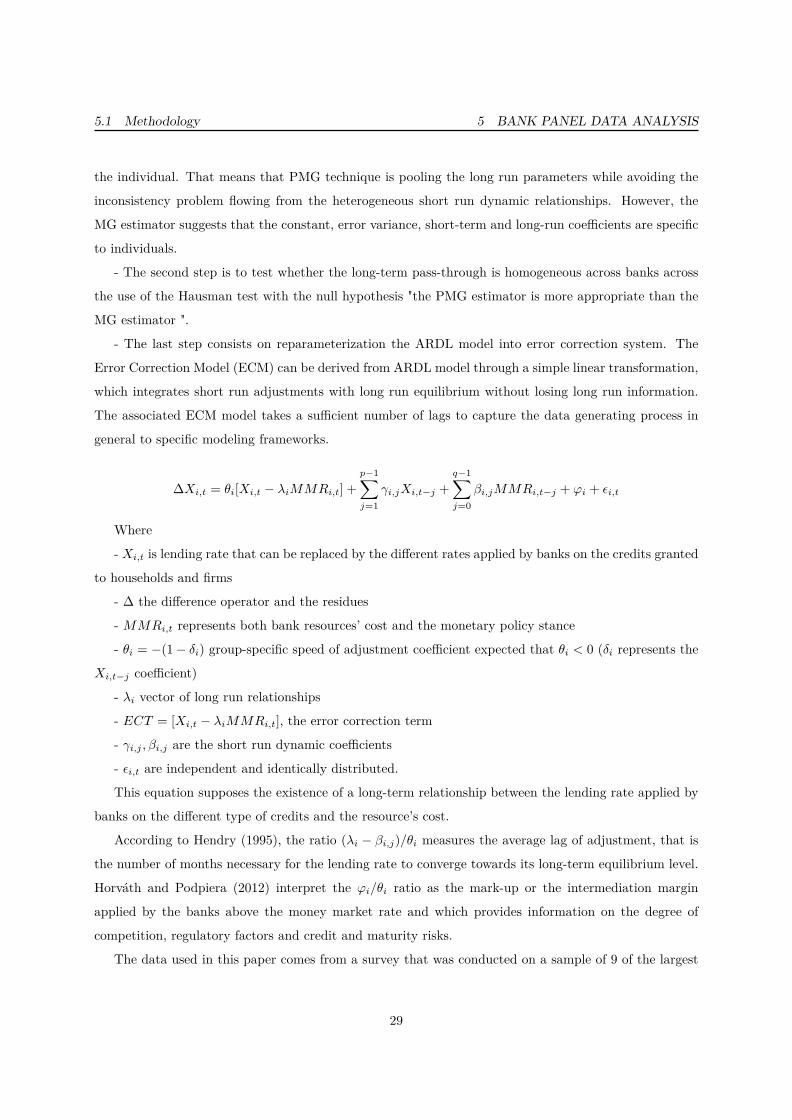
- The last step consists on reparameterization the ARDL model into error correction system. The
Error Correction Model (ECM) can be derived from ARDL model through a simple linear transformation,
which integrates short run adjustments with long run equilibrium without losing long run information.
The associated ECM model takes a sufficient number of lags to capture the data generating process in
general to specific modeling frameworks.
∆Xi,t = θi[Xi,t − λiMMRi,t] +p−1∑j=1
γi,jXi,t−j +q−1∑j=0
βi,jMMRi,t−j + ϕi + εi,t
Where
- Xi,t is lending rate that can be replaced by the different rates applied by banks on the credits granted
to households and firms
- ∆ the difference operator and the residues
- MMRi,t represents both bank resources’ cost and the monetary policy stance
- θi = −(1 − δi) group-specific speed of adjustment coefficient expected that θi < 0 (δi represents the
Xi,t−j coefficient)
- λi vector of long run relationships
- ECT = [Xi,t − λiMMRi,t], the error correction term
- γi,j , βi,j are the short run dynamic coefficients
- εi,t are independent and identically distributed.
This equation supposes the existence of a long-term relationship between the lending rate applied by
banks on the different type of credits and the resource’s cost.
According to Hendry (1995), the ratio (λi − βi,j)/θi measures the average lag of adjustment, that is
the number of months necessary for the lending rate to converge towards its long-term equilibrium level.
Horváth and Podpiera (2012) interpret the ϕi/θi ratio as the mark-up or the intermediation margin
applied by the banks above the money market rate and which provides information on the degree of
competition, regulatory factors and credit and maturity risks.
The data used in this paper comes from a survey that was conducted on a sample of 9 of the largest
29
5.2 Variables’ Definitions and Data Sources 5 BANK PANEL DATA ANALYSIS
Tunisian banks on a monthly basis since January 2012 till December 2018. It provides information on
the lending rates applied to new loans.
5.2 Variables’ Definitions and Data Sources
This section describes the sources and definitions of data. To assess the impact of monetary policy
decision on the banks’ behavior in terms of pricing policy, the following data 22 was used:
Variables Definition SourceMoney It reflects, at the same time, the monetary policy stance and the
Market Rate bank resource’s cost. CBTLending It represents the pricing policy. It was introduced by agent and by
maturity of credit (households/firms, less than 3 years/ between 3 CBTrates and 7years/ more than 7 years).
5.3 Results and interpretation
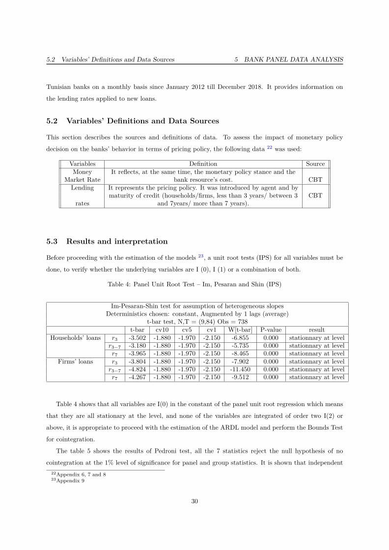
Before proceeding with the estimation of the models 23, a unit root tests (IPS) for all variables must be
done, to verify whether the underlying variables are I (0), I (1) or a combination of both.
Table 4: Panel Unit Root Test – Im, Pesaran and Shin (IPS)
Im-Pesaran-Shin test for assumption of heterogeneous slopesDeterministics chosen: constant, Augmented by 1 lags (average)
t-bar test, N,T = (9,84) Obs = 738t-bar cv10 cv5 cv1 W[t-bar] P-value result
Households’ loans r3 -3.502 -1.880 -1.970 -2.150 -6.855 0.000 stationnary at levelr3−7 -3.180 -1.880 -1.970 -2.150 -5.735 0.000 stationnary at levelr7 -3.965 -1.880 -1.970 -2.150 -8.465 0.000 stationnary at level
Firms’ loans r3 -3.804 -1.880 -1.970 -2.150 -7.902 0.000 stationnary at levelr3−7 -4.824 -1.880 -1.970 -2.150 -11.450 0.000 stationnary at levelr7 -4.267 -1.880 -1.970 -2.150 -9.512 0.000 stationnary at level
Table 4 shows that all variables are I(0) in the constant of the panel unit root regression which means
that they are all stationary at the level, and none of the variables are integrated of order two I(2) or
above, it is appropriate to proceed with the estimation of the ARDL model and perform the Bounds Test
for cointegration.
The table 5 shows the results of Pedroni test, all the 7 statistics reject the null hypothesis of no
cointegration at the 1% level of significance for panel and group statistics. It is shown that independent22Appendix 6, 7 and 823Appendix 9
30

5.3 Results and interpretation 5 BANK PANEL DATA ANALYSIS
Table 5: The Pedroni Panel Cointegration Test
Households’ loans Firms’ loansTest less between more less between
than 3 3 and 7 than 7 than 3 3 and 7years years years years years
Panel υ-Statistic 5,954 5,442 6,969 5,066 9,485Panel β-Statistic -20,34 -12,83 -15,68 -21,09 -34,47
Panel t-Statistic (non-parametric) -11,44 -8,303 -10,8 -12,82 -17,36Panel t-Statistic (adf): (parametric) -3,499 -4,892 -6,668 -5,166 -10,95
Group β–Statistic -18,59 -11,92 -15,83 -21,48 -31,41Group t-Statistic (non-parametric) -12,49 -9,123 -12,79 -15,46 -19,79Group t-Statistic (adf): (parametric) -3,677 -4,8 -6,762 -5,264 -10,94
Note: All test statistics are distributed N(0,1), under a null of no cointegration
variables do hold cointegration in the long run for the 9 banks with respect to lending rates.
Ultimately, the use of an Error Correction Model (ECM) is justified since the cointegration test
confirms the existence of a relationship of long term between lending rates on one hand and the money
market rate on the other hand. In order to select the appropriate model of the long run underlying
equation, we determined the optimum lag length (k) by using the Akaike Information Criterion(AIC).
Table 6 represents the results of the Mean Group (MG) and Pooled Mean Group (PMG) estimators’
models in order to ensure the robustness of results. These two approaches which emphasize the mark-
up, short-term and long-term pass-through and average lag of adjustment 24, confirm the results of the
Pedroni’s cointegration test. In other words, there is an equilibrium relationship between the lending rates
applied by banks on the different type of credits and the money market rate at 1% level. In addition, the
coefficient that measures the speed of adjustment is significant with a negative sign.
It should be noted that first, for loans which the maturity exceeded 7 years and which are granted
to firms, the estimation results for both PMG and MG are not significant that can be explained by the
fact that for this last type of credit, banks on who’s the survey was conducted are not very active in
this sector. Second, for loans which the maturity is less than 3 years, the estimations were applied on a
shorter period (from November 2013 till December 2018). This initiative was undertaken due to a specific
problem to one of the banks.
Although both PMG and MG are consistent, Hausman specification test 25 which aims to check for
heterogeneity among the long run equation parameters between these two models does not reject the
assumption that the PMG estimator can’t be used. That is to say, MG is inefficient, and PMG is chosen
for the final estimation, thus banks adopt the same long-term pricing policy for all type of credits.24It should be noted that the presented coefficients are aggregated. These correspond to the averages of the specific
coefficients to each bank weighted by their respective estimated covariances.25Appendix 10
31

5.3 Results and interpretation 5 BANK PANEL DATA ANALYSIS
Table 6: Results of pass-through estimates
Estimation results of PMG Estimation results of MGHouseholds’ loans Firms’ loans Households’ loans Firms’ loans
less between more less between less between more less betweenthan 3 3 and 7 than 7 than 3 3 and 7 than 3 3 and 7 than 7 than 3 3 and 7years years years years years years years years years years
Constant ϕi 0,47 1,31 0,51 1,12 0,25 0,50 1,52 0,56 1,31 0,25[0,000] [0,000] [0,000] [0,000] [0,000] [0,004] [0,000] [0,000] [0,000] [0,000]
Short termPass- 0,20 0,24 0,22 0,27 0,29 0,18 0,24 0,22 0,26 0,29
through βi,j [0,306] [0,002] [0,021] [0,018] [0,098] [0,349] [0,002] [0,021] [ 0,022] [0,000]speed of
adjustement 0,13 0,37 0,14 0,59 0,12 0,14 0,41 0,14 0,66 0,12θi [0,000] [0,000] [0,000] [0,000] [0,000] [0,000] [0,000] [0,000] [0,000] [0,110]
Long termPass- 0,98 0,95 0,82 0,99 1,06 0,81 0,94 0,74 1,00 1,10
through λi [0,000] [0,000] [0,000] [0,000] [0,000] [0,000] [0,000] [0,000] [0,000] [0,016]Averagelag of
adjustement 6 2 5 2 7 5 2 4 2 7Mark up 3,50 3,57 3,74 1,89 2,09 3,53 3,68 3,90 1,97 1,99Relative
adjustement 0,13 0,35 0,11 0,58 0,13 0,11 0,39 0,11 0,66 0,14Note: The p-values are [between]. We present only the aggregated coefficients that are the
averages of the coefficients specific to each bank weighted by their respective estimated covariances
Households’ loans:
Based on the results of the PMG model estimates, the long-term pass-through is almost complete for
all type of loans granted to households. In other words the money market rate has a long run impact on
the households’ lending rates at 1% level. The pass-through coefficients are presented as follow: 98% for
the consumer credit, 95% for the housing sitting out credit and 82% for the housing loans.
As concern short-term pass-through, PMG estimator confirms that the money market rate has a short
run impact on the households’ lending rate for the housing sitting out credit and the housing credit at 1%
level. However, it’s not the case for the consumer credit since its short term coefficient is not significant.
That suggests that banks are not changing instantly consumer credit’s rate following a monetary policy
decision may be for two reasons: the lower risk incurred on this type of credit, and the relative comfortable
margin that allows banks to reduce it with the aim to preserve their competitiveness.
Similarly, average lag of adjustment for households’ lending rates towards long-term equilibrium due
to changes in banks’ refinancing conditions are generally short and depend on the business’s line. We can
find that the convergence period for consumer and housing credit’s rates, respectively 6 and 5 months; it
is relatively shorter for the housing sitting out credit with 2 months. That can be explained by the fact
32

6 CONCLUSION
that almost of the housing loans are granted at a fixed rate.
Firms’ loans:
Based on the results of the PMG model estimates, the long-term pass-through is complete for the
medium term credits with 106% as a pass-through coefficient and almost complete for management credits.
That confirms that the money market rate has a long run impact on the firms’ lending rate.
As concern short-term pass-through, PMG estimator confirms that the money market rate has a short
run impact on the firms’ lending rate for the management and the equipment acquisition and extension
credit at 1% level.
Similarly, average lag of adjustment for firms’ lending rates towards long-term equilibrium due to
changes in banks’ refinancing conditions is a little bit specific. For the management credit, the convergence
period is about 2 months. This is due to the fact that there is a strong competition on this type of credit,
which, as already outlined, it represents 53% of the whole distributed loans. For the medium credit, the
convergence period is longer. It takes 7 month to adjust towards long-term equilibrium. That can be
explained by the firms’ bargaining power which creates a certain rigidity regarding the monetary policy’s
changes.
With regards to the mark-up rates applied by the banks, it appears that the households’ intermediation
margins are relatively more important than those applied to firms. However, we can say that the firm’s
mark-up policy is changing (not constant) which explain the complete long-term pass-through for the
management and the medium term credits.
Hence, banks transmit any changes in the MMR to lending rates applied to households
as well as to firms. This significant rates’ adjustment could be explained by the strong
indexation of lending rates to MMR. The results reveal also that the MMR hasn’t a short
run impact on the consumer credit and it seems that banks choose to not transmit, especially
an increase of MMR, to this type of credit since it is characterised by a lower risk and a
relative comfortable margin with the aim to preserve their competitiveness. it was found
also that the lending rates applied to the equipment acquisition and extension credit for
firms and housing credits for households are more or less rigid to a change in the MMR
compared to other credit categories. This limited adjustment could be explained by the
above-mentioned specificities of these two types of credit.
6 Conclusion
In this paper two approaches were considered in assessing the interest rate and credit transmission chan-
nels. The first approach is based on an aggregate data analysis. Structural Vector Auto regressive (SVAR)
33
6 CONCLUSION
was employed with a quarterly data since 2000 till June 2018 to assess the impact and the delay of mone-
tary policy decisions and to identify through which of the two channels monetary policy stance’s changes
could affect the real economy.
It was found that the monetary policy action could explain to a large extent the evolution of lending
rates and to a lesser degree the evolution of banks’ lending, especially after the Revolution. This seems
evident as the lending rates are strongly indexed to MMR. For the real activity, an important contribution
of the monetary policy action in explaining the evolution of both GDP growth and core inflation was
noticed.
Moreover, the lending rates could explain the variability of both GDP growth and core inflation
better than the credits’ volume, and within a short time frame (the transmission is observed from the
8th quarter with a large value) thanks to the high dependence of the banks’ pricing policy on the MMR
level, especially after the revolution.
Therefore, the interest rate channel has a bigger influence on the real activity in comparison with the
credit channel, even though this latter begins to hold much promise in explaining the macroeconomics
variables.
The second approach is based on a bank panel data analysis. An ARDL model was used with a
monthly data since 2012 till 2018 to measure the reaction of the banks’ pricing policy to monetary policy
changes.
It was found that banks’ pricing policy is highly dependent on the monetary policy stances. They
transmit any changes in the money market rate to lending rates applied to households as well as to firms.
That could be explained by the strong indexation of lending rates to MMR. The results reveal also that
the money market rate hasn’t a short run impact on the consumer credit and it seems that banks choose
to not transmit, especially an increase of MMR, to this type of credit since it is characterised by a lower
risk and a relative comfortable margin with the aim to preserve their competitiveness. it was found also
that the lending rates applied to the equipment acquisition and extension credit for firms and housing
credits for households are more or less rigid to a change in the MMR compared to other credit categories.
34
7 APPENDIX
7 Appendix
Appendix 1: Historical overview of the Tunisian banking landscape
- In the aftermath of independence, the foundations of a Tunisian banking system were put in place with
the creation in 1958 of the Central Bank of Tunisia (BCT) and the Tunisization of the system banking.
Thus, the Tunisian Bank Corporation (STB, 1957), the Société Nationale d’Investissement (SNI, 1958)
and the National Agricultural Bank (BNA, 1959)
- Since 1980: Financial Reforms and Internationalization of Banking Capital
- June 1989: The Housing Bank (BH) was born following the transformation of the Caisse Nationale
Savings Bank (CNEL) in universal banking
- 1997: Privatization of the Banque du Sud following the State’s renunciation of its right to subscription
to the capital increase of the bank reducing the public participation of 36% to 32%. In 2005, the State’s
residual stake was transferred to the Banco consortium. Santander and AttijariWafa Bank, which acquired
53% of the capital of the bank named now "ATTIJARI BANK"
- January 1998: Entry into force of the Tunisian Bank of Solidarity (BTS)
- December 2000: Absorption of the Tunisian Economic Development Bank (BDET) and of the
National Bank for Tourism Development (BNDT) by the STB
- 2002: Privatization of the International Union of Banks (UIB) by the sale of 52% of its capital at
Société Générale
- 2007: Privatization of the BTK (Tunisian-Kuwaiti Bank) by the sale of 60% of its capital (30%
of the Tunisian State and 30% of the Kuwaiti State) to the "Financière OCÉOR" subsidiary of Groupe
BPCE
- March 2005: Start of operation of the Small and Medium Enterprise Finance Bank (BFPME)
- 2010: Entry of the Zitouna bank specializing in Islamic finance
- 2012: Opening of an office of the European Bank for Reconstruction and Development (EBRD)
35

7 APPENDIX
SVAR model
Table 7: Appendix 2: Descriptive Statistics of the different variables
NGDPHA Core_inf MMR RR Lendingrate
RatioLoansto GDP
LNPL NEER
Mean 0.007703 0.035660 0.048768 0.016646 0.075240 0.689963 -1.492140 4.636686Median 0.008884 0.031969 0.050000 0.014242 0.075163 0.629892 -1.702403 4.636277
Maximum 0.030128 0.076811 0.065367 0.058499 0.094982 1.171906 -0.689998 4.937491Minimum -0.043378 0.011268 0.032367 0.000000 0.054083 0.009650 -2.077626 4.197453Std. Dev. 0.010166 0.016910 0.006584 0.014191 0.009522 0.397251 0.448735 0.199699
Table 8: Appendix 3: Unit Root Test results
Kwiatkowski-Phillips-Schmidt-ShinIntercept Intercept & Trend
NGDPHA 0.494050* 0.058013***Core_inf 1.070480 0.069727***MMR 0.594844* 0.190627*RR 0.234545*** 0.233353
Lending rate 0.775618 0.214915*Ratio loans to GDP 1.099814 0.105006***
LNPL 1.052746 0.201500*NEER 1.148919 0.1211263**
*, ** & *** denote 1%, 5% & 10% significant levels respectively
36

7 APPENDIX
Table 9: Appendix 4: SVAR lags order selection
VAR Lag Order Selection CriteriaLag LogL LR FPE AIC SC HQ0 742.7314 NA 1.83e-19 -23.28166 -22.56118 -22.998781 1157.331 695.4574 1.41e-24 -35.07519 -32.67359* -34.132262 1220.446 91.61849 9.68e-25 -35.53051 -31.44779 -33.927533 1259.578 47.96797 1.62e-24 -35.21218 -29.44834 -32.949154 1357.140 97.56216* 5.01e-25 -36.77871 -29.33374 -33.855625 1422.553 50.64220 6.05e-25 -37.30815 -28.18206 -33.725026 1514.707 50.53609 5.56e-25 -38.70022 -27.89300 -34.457037 1702.070 60.43989 8.43e-26* -43.16356* -30.67522 -38.26033** indicates lag order selected by the criterionLR: sequential modified LR test statistic (each test at 5% level)FPE: Final prediction errorAIC: Akaike information criterionSC: Schwarz information criterionHQ: Hannan-Quinn information criterion
Table 10: Appendix 5: Estimated Contemporaneous Effects
2000q1-2010q4 2011q1-2018q20,008 0 0 0 0 0 0 0,006 0 0 0 0 0 0-0,001 0,003 0 0 0 0 0 0 0,003 0 0 0 0 0
0 0 0,003 0 0 0 0 0 0,001 0,001 0 0 0 00 0 0,001 0,002 0 0 0 0 0,001 0,002 0,001 0 0 0
-0,003 0,008 0,001 -0,003 0,037 0 0 -0,007 0 -0,005 0,003 0,003 0 00,01 -0,004 -0,015 0 -0,045 0,042 0 -0,016 -0,006 0,01 -0,009 -0,002 0,022 00 0,002 0 0,001 0 -0,001 0,007 0,01 -0,006 -0,001 0,006 -0,006 -0,002 0,018
37

7 APPENDIX
ARDL model
Table 11: Appendix 6: Descriptive statistics
Variable Obs Mean Std. Dev. Min MaxHouseholds’ loans r_3 756 8,012 0,99 4,52 10,738
r_3-7 756 7,956 0,889 4,282 10,489r_7 756 7,466 0,817 4,82 10,176
Firms’ loans r_3 756 6,511 0,986 3,996 9,68r_3-7 756 6,995 1,038 4,04 10,945r_7 756 5,027 3,316 0 12,504
MMR 756 4,81 0,91 3,16 7,25
Table 12: Appendix 7: Correlation analysis
Households’ Firms’ MMRloans loans
r_3 r_3-7 r_7 r_3 r_3-7 r_7Households’ loans r_3 1Households’ loans r_3-7 0,7414 1Households’ loans r_7 0,6174 0,8458 1
Firms’ loans r_3 0,6913 0,8622 0,8133 1Firms’ loans r_3-7 0,681 0,8608 0,7824 0,8425 1Firms’ loansr_7 0,2904 0,1769 0,2233 0,2906 0,2055 1
MMR 0,7217 0,8773 0,7967 0,8622 0,8265 0,139 1
Table 13: Appendix 8: Optimal lag selection
Households’ loans Firms’ loansvaraibles lag varaibles lag
loans – 3 years r_3 2 loans – 3 years r_3 2MMR 0 MMR 2
loans 3-7 years r_3-7 1 loans 3-7 years r_3-7 2MMR 2 MMR 1
loans + 7 years r_7 2 loans + 7 years r_7 1MMR 2 MMR 0
Appendix 9: Estimation Procedure
- IM, Pesaran and Shin for unit root
IPS estimates the t-test for unit roots in heterogeneous panels developed by Im, Pesaran and Shin
(IPS, 2003). It allows for individual effects, time trends, and common time effects. Based on the mean
of the individual Dickey-Fuller t-statistics of each unit in the panel, the IPS test assumes that all series
38
7 APPENDIX
are non-stationary under the null hypothesis. Lags of the dependent variable may be introduced to allow
for serial correlation in the errors.
Im, Pesaran and Shin denoted IPS proposed a test for the presence of unit roots in panels that
combines information from the time series dimension with that from the cross section dimension, such
that fewer time observations are required for the test to have power. Since the IPS test has been found
to have superior test power by researchers in economics to analyze long-run relationships in panel data,
we will also employ this procedure in this study.
- Panel Cointegration Tests
Cointegration is an econometric concept that mimics the existence of a long-run equilibrium among
underlying economic time series that converges over time. Thus, cointegration establishes a stronger
statistical and economic basis for empirical error correction model, which brings together short and long-
run information in modeling variables.
Non-cointegrating tests on panel data proposed by Pedroni (1995, 1997, 1999, 2003), Kao (1999) and
Bai and Ng (2001) are residual tests analogous to the proposed tests by Engle and Granger (1987) in the
context of time series.
Pedroni (1995, 1997) proposed various tests with the aim of to apprehend the null hypothesis of
absence intra-individual cointegration for both homogeneous and heterogeneous panels. Just like the
unit root tests of Im, Pesaran and Shin (2003), Pedroni’s tests take heterogeneity into account through
parameters that may differ between individuals. Such heterogeneity may be both at the level of the
cointegration relations, and at the level of the short-term dynamics.
Thus, under the alternative hypothesis, there is a cointegration relation for each individual, and this
cointegrating relationship is not necessarily the same for each individual of the panel. Taking into account
such heterogeneity is an undeniable advantage since, in practice; it is rare for cointegration vectors to
be identical from one individual to another on the panel. In these circumstances, erroneously imposing
homogeneity of the cointegrating vectors would result in the non-rejection of the null hypothesis of absence
of cointegration, even though the variables are cointegrated.
- Determination of the Existence of the Long Run Relationship of the Variables
The long run relationship of the underlying variables is detected through the Hausman test. The
Hausman Test (also called the Hausman specification test) detects endogenous regressors (predictor vari-
ables) in a regression model. Endogenous variables have values that are determined by other variables in
the system.
A Hausman statistic is constructed as a function of the difference between the two estimators: Mean
Group (MG) and Pooled Mean Group (PMG). The sampling distribution of the Hausman statistic de-
termines how big a difference is too big to be compatible with the null hypothesis of correct specification.
39
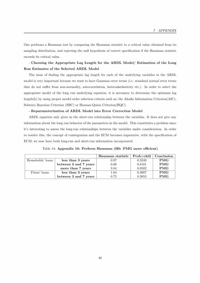
7 APPENDIX
One performs a Hausman test by comparing the Hausman statistic to a critical value obtained from its
sampling distribution, and rejecting the null hypothesis of correct specification if the Hausman statistic
exceeds its critical value.
- Choosing the Appropriate Lag Length for the ARDL Model/ Estimation of the Long
Run Estimates of the Selected ARDL Model
The issue of finding the appropriate lag length for each of the underlying variables in the ARDL
model is very important because we want to have Gaussian error terms (i.e. standard normal error terms
that do not suffer from non-normality, autocorrelation, heteroskedasticity etc.). In order to select the
appropriate model of the long run underlying equation, it is necessary to determine the optimum lag
length(k) by using proper model order selection criteria such as; the Akaike Information Criterion(AIC),
Schwarz Bayesian Criterion (SBC) or Hannan-Quinn Criterion(HQC).
- Reparameterization of ARDL Model into Error Correction Model
ARDL equation only gives us the short-run relationship between the variables. It does not give any
information about the long run behavior of the parameters in the model. This constitutes a problem since
it’s interesting to assess the long-run relationships between the variables under consideration. In order
to resolve this, the concept of cointegration and the ECM becomes imperative, with the specification of
ECM; we now have both long-run and short-run information incorporated.
Table 14: Appendix 10: Perform Hausman (H0: PMG more efficient)
Hausman statistic Prob>chi2 ConclusionHouseholds’ loans less than 3 years 0.97 0.3249 PMG
between 3 and 7 years 0.06 0.8101 PMGmore than 7 years 3.84 0.0502 PMG
Firms’ loans less than 3 years 1.64 0.2007 PMGbetween 3 and 7 years 0.75 0.3853 PMG
40

8 BIBLIOGRAPHY
8 Bibliography
Blanchard, O. J., & Quah, D. (1988). The dynamic effects of aggregate demand and supply disturbances.
Bernanke, B. S., & Mihov, I. (1998). Measuring monetary policy. The quarterly journal of economics,
113(3), 869-902.
Bernanke, B. S. (1986). Alternative explanations of the money-income correlation.
Boivin, J., & Giannoni, M. (2002). Assessing changes in the monetary transmission mechanism: A
VAR approach. Federal Reserve Bank of New York Economic Policy Review, 8(1), 97-111.
Ilzetzki, E., Reinhart, C. M., & Rogoff, K. S. (2017). Exchange arrangements entering the 21st
century: Which anchor will hold? (No. w23134). National Bureau of Economic Research.
Mishkin, F. S. (1996). The channels of monetary transmission: lessons for monetary policy (No.
w5464). National Bureau of Economic Research.
Taylor, J. B. (1995). The monetary transmission mechanism: an empirical framework. journal of
Economic Perspectives, 9(4), 11-26.
Bernanke, B. (1990). The federal funds rate and the channels of monetary transnission (No. w3487).
National Bureau of Economic Research.
Gitonga, M. V. (2015). Analysis of Interest Rate Channel of Monetary Transmission Mechanism in
Kenya. International Journal of Business and Commerce, 4(4), 38-67.
Barran, F., Coudert, V., & Mojon, B. (1995). Transmission de la politique monétaire et crédit bancaire
Une application à trois pays de l’OCDE. Revue économique, 393-413.
Kohlscheen, E., & Miyajima, K. (2015). The transmission of monetary policy in EMEs in a changing
financial environment: a longitudinal analysis.
Ireland, P. N. (2010). Monetary transmission mechanism. In Monetary Economics (pp. 216-223).
Palgrave Macmillan, London.
Christiano, L. J., Eichenbaum, M., & Evans, C. L. (2005). Nominal rigidities and the dynamic effects
of a shock to monetary policy. Journal of political Economy, 113(1), 1-45.
Samkharadze, B. (2008). Monetary transmission mechanism in Georgia: analyzing pass-through of
different channels. National Bank of Georgia Working Paper, 2, 2008.
Ndubuisi, G. O. (2015). Interest Rate Channel of Monetary Policy Transmission Mechanisms: What
Do We Know About it?. Available at SSRN 2623036.
Kelikume, I. (2014). Interest Rate Channel of Monetary Transmission Mechanism: Evidence from
Nigeria. The International Journal of Business and Finance Research, 8(4), 97-107.
Wulandari, R. (2012). Do credit channel and interest rate channel play important role in monetary
transmission mechanism in Indonesia?: A structural vector autoregression model. Procedia-Social and
Behavioral Sciences, 65, 557-563.
41

8 BIBLIOGRAPHY
Çavuşoğlu, A. T. (2002). Credit transmission mechanism in Turkey: an empirical investigation.
Middle East Technical University ERC Working Papers in Economics, 2(03), 1-30.
Bennouna, H. (2018). Pass-through du taux d’intérêt au Maroc: Enseignements à partir de l’enquête
trimestrielle sur les taux débiteurs (No. 2018-4). Bank Al-Maghrib, Département de la Recherche.
Nkoro, E., & Uko, A. K. (2016). Autoregressive Distributed Lag (ARDL) cointegration technique:
application and interpretation. Journal of Statistical and Econometric Methods, 5(4), 63-91.
Asongu, S., El Montasser, G., & Toumi, H. (2016). Testing the relationships between energy con-
sumption, CO 2 emissions, and economic growth in 24 African countries: a panel ARDL approach.
Environmental Science and Pollution Research, 23(7), 6563-6573.
42


