

Association Rule Mining
Debapriyo Majumdar
Data Mining – Fall 2014
Indian Statistical Institute Kolkata
August 4 and 7, 2014
2
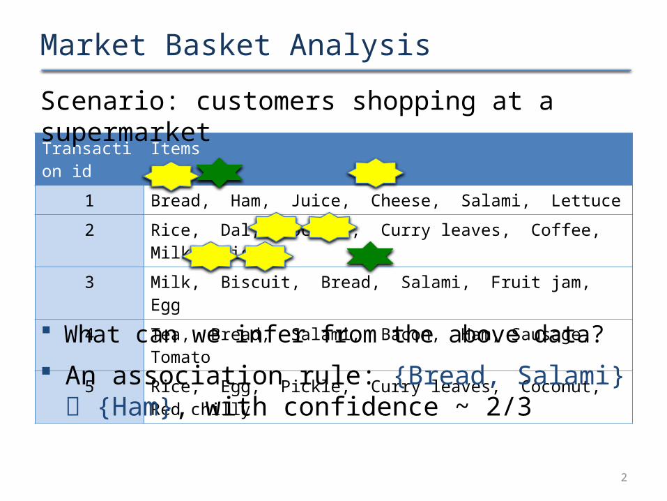
Transaction id
Items
1 Bread, Ham, Juice, Cheese, Salami, Lettuce
2 Rice, Dal, Coconut, Curry leaves, Coffee, Milk, Pickle
3 Milk, Biscuit, Bread, Salami, Fruit jam, Egg
4 Tea, Bread, Salami, Bacon, Ham, Sausage, Tomato
5 Rice, Egg, Pickle, Curry leaves, Coconut, Red chilly
Market Basket Analysis
Scenario: customers shopping at a supermarket
What can we infer from the above data? An association rule: {Bread, Salami} {Ham}, with
confidence ~ 2/3

3
Applications Information driven marketing Catalog design Store layout Customer segmentation based on buying patterns
Several papers by Rakesh Agrawal and others in the 1990s
Rakesh Agrawal and Ramakrishnan Srikant
Fast Algorithms for Mining Association Rules
The VLDB 1994
4
The Market-Basket Model A (large) set of binary attributes, called items
I = {i1, …, in}
e.g. milk, bread, the items sold at the market
A transaction T consists of a (small) subset of I
e.g. the list of items (bill) bought by one customer at once
The database D is a (large) set of transactions
D = {T1, …, TN}
5
The Market-Basket Model Goal: mining associations between the items– The transactions or customers also may have associations,
but here we are interested in such relations
Approach: finding subset of items that are present together in transactions frequently
An itemset: any subset X of I
6
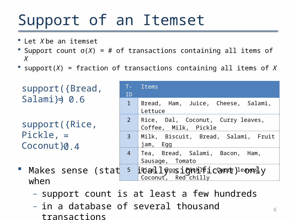
Support of an Itemset Let X be an itemset Support count σ(X) = # of transactions containing all items of X support(X) = fraction of transactions containing all items of X
Makes sense (statistically significant) only when – support count is at least a few hundreds– in a database of several thousand transactions
support({Bread, Salami})
support({Rice, Pickle, Coconut})
= 0.6
= 0.4
T-ID Items
1 Bread, Ham, Juice, Cheese, Salami, Lettuce
2 Rice, Dal, Coconut, Curry leaves, Coffee, Milk, Pickle
3 Milk, Biscuit, Bread, Salami, Fruit jam, Egg
4 Tea, Bread, Salami, Bacon, Ham, Sausage, Tomato
5 Rice, Egg, Pickle, Curry leaves, Coconut, Red chilly
7
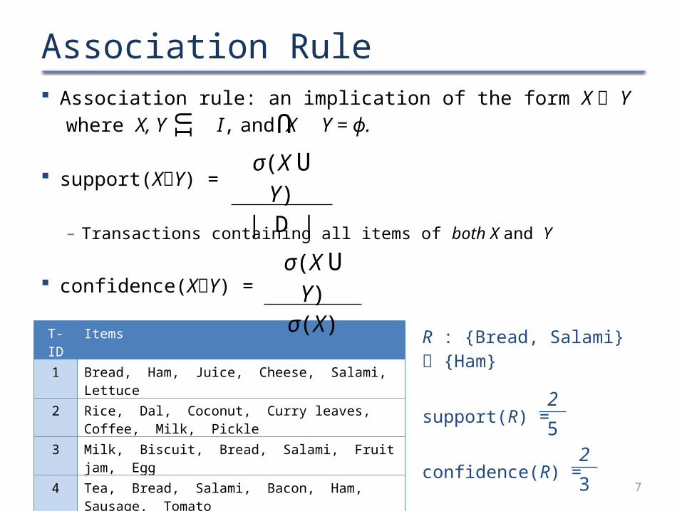
Association Rule Association rule: an implication of the form X Y
where X, Y I, and X Y = ϕ.
support(XY) =
– Transactions containing all items of both X and Y
confidence(XY) =
UUI
T-ID Items
1 Bread, Ham, Juice, Cheese, Salami, Lettuce
2 Rice, Dal, Coconut, Curry leaves, Coffee, Milk, Pickle
3 Milk, Biscuit, Bread, Salami, Fruit jam, Egg
4 Tea, Bread, Salami, Bacon, Ham, Sausage, Tomato
5 Rice, Egg, Pickle, Curry leaves, Coconut, Red chilly
σ(X U Y)
| D |
σ(X U Y)
σ(X)
R : {Bread, Salami} {Ham}
support(R) =
confidence(R) =
2
52
3
8
Association Rule Mining Task Given a set of items I, a set of transactions D, a
minimum support thresholds minsup and a minimum confidence threshold minconf
Find all rules R such that
support(R) ≥ minsup
confidence(R) ≥ minconf
9
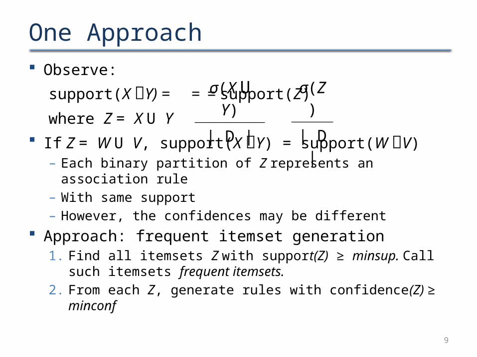
One Approach Observe:
support(X Y) = == support(Z)
where Z = X U Y If Z = W U V, support(X Y) = support(W V)
– Each binary partition of Z represents an association rule– With same support– However, the confidences may be different
Approach: frequent itemset generation1. Find all itemsets Z with support(Z) ≥ minsup. Call such itemsets
frequent itemsets.
2. From each Z, generate rules with confidence(Z) ≥ minconf
σ(X U Y)
| D |σ(Z)
| D |

10
Finding Frequent Itemsets If | I | = n, then number of possible itemsets = 2n
For each itemset, compute the support by scanning the lists of items of each transaction– O(N × w), where w is the average length of transactions
Overall complexity: O(2n× N × w) Computationally very expensive!!
11
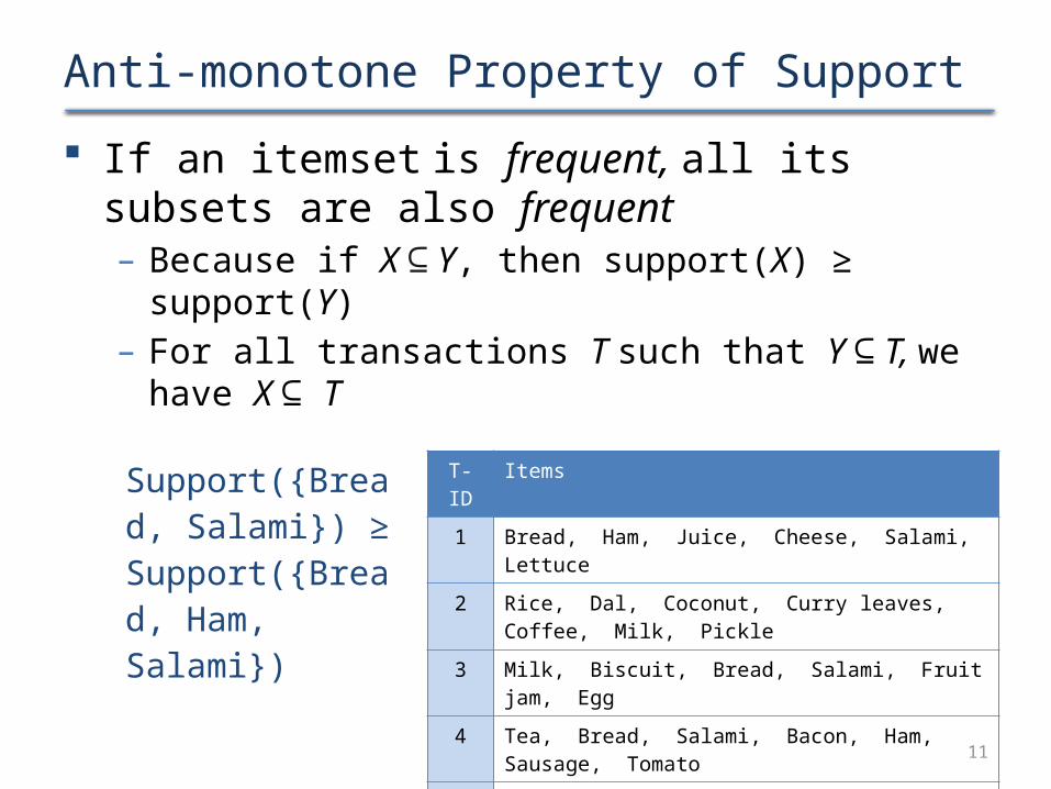
Anti-monotone Property of Support If an itemset is frequent, all its subsets are also
frequent– Because if X ⊆ Y, then support(X) ≥ support(Y)– For all transactions T such that Y ⊆ T, we have X ⊆ T
T-ID Items
1 Bread, Ham, Juice, Cheese, Salami, Lettuce
2 Rice, Dal, Coconut, Curry leaves, Coffee, Milk, Pickle
3 Milk, Biscuit, Bread, Salami, Fruit jam, Egg
4 Tea, Bread, Salami, Bacon, Ham, Sausage, Tomato
5 Rice, Egg, Pickle, Curry leaves, Coconut, Red chilly
Support({Bread, Salami}) ≥ Support({Bread, Ham, Salami})

12
The A-Priori AlgorithmNotation:
Lk = The set of frequent (large) itemsets of size k
Ck= The candidate set of frequent (large) itemsets of size.
Algorithm:
L1 = {Frequent 1-itemsets};
for ( k = 2; Lk – 1 ≠ 0; k++ ) do begin
Ck = apriori_gen(Lk-1); /* Generating new candidates */
for all transactions T in D do begin
CT = subset(Ck,T) /* Keeping only the valid candidates */
for all candidates c in CT do
c.count++;
end
Lk = {c in Ck | c.count ≥ minsup}
end
Output = Union of all Lk for k = 1, 2, … , n
13
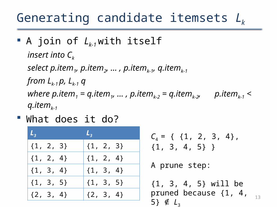
Generating candidate itemsets Lk
A join of Lk-1 with itself
insert into Ck
select p.item1, p.item2, … , p.itemk-1, q.itemk-1
from Lk-1 p, Lk-1 q
where p.item1 = q.item1, … , p.itemk-2 = q.itemk-2, p.itemk-1 < q.itemk-1
What does it do?L3 L3
{1, 2, 3} {1, 2, 3}
{1, 2, 4} {1, 2, 4}
{1, 3, 4} {1, 3, 4}
{1, 3, 5} {1, 3, 5}
{2, 3, 4} {2, 3, 4}
C4 = { {1, 2, 3, 4}, {1, 3, 4, 5} }
A prune step:
{1, 3, 4, 5} will be pruned because {1, 4, 5} ∉ L3
14
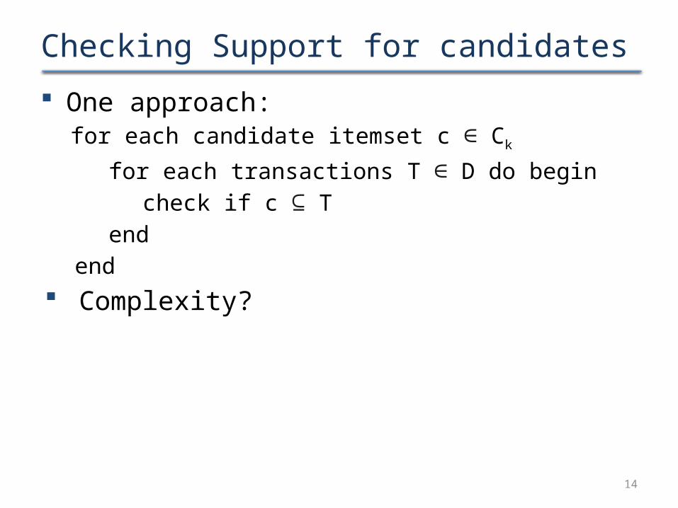
Checking Support for candidates One approach:
for each candidate itemset c ∈ Ck
for each transactions T ∈ D do begin
check if c ⊆ T
end
end
Complexity?
15
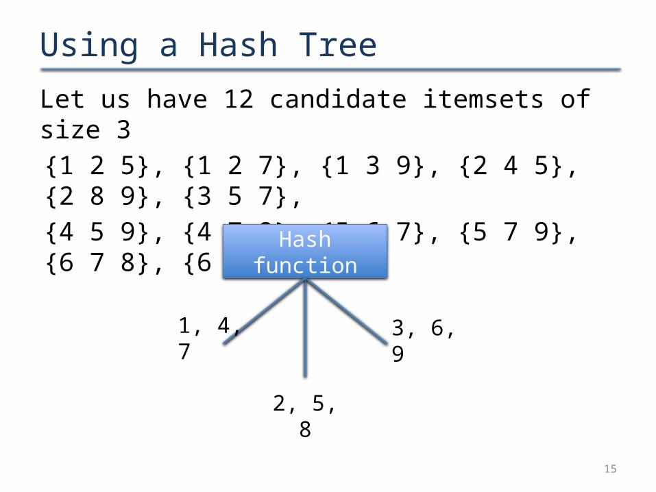
Using a Hash TreeLet us have 12 candidate itemsets of size 3
{1 2 5}, {1 2 7}, {1 3 9}, {2 4 5}, {2 8 9}, {3 5 7},
{4 5 9}, {4 7 8}, {5 6 7}, {5 7 9}, {6 7 8}, {6 7 9}
Hash function
1, 4, 7
2, 5, 8
3, 6, 9
16
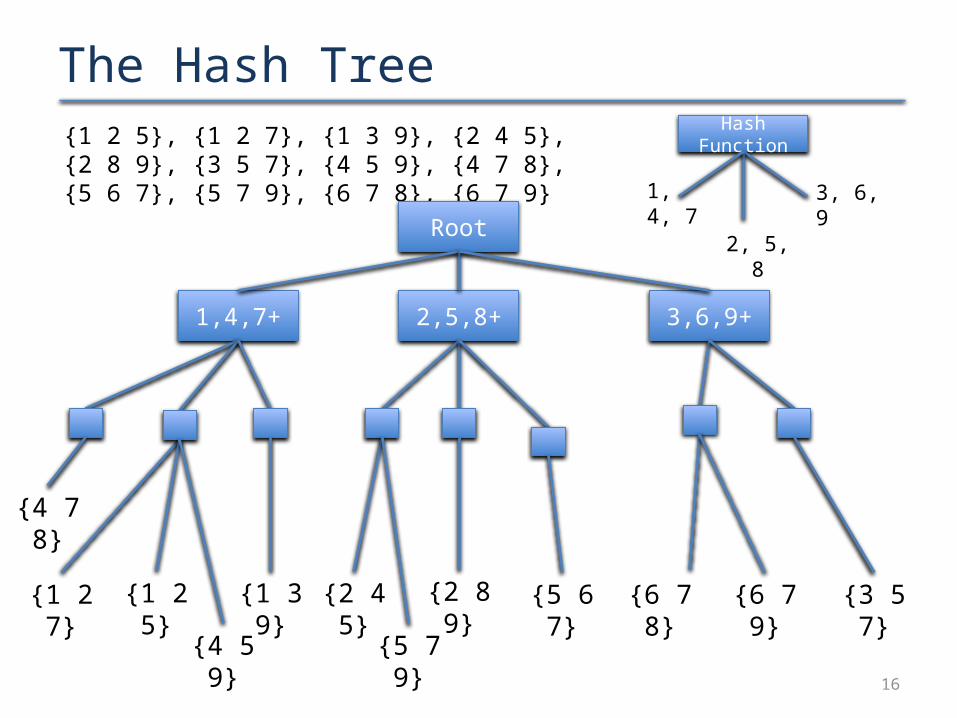
The Hash Tree{1 2 5}, {1 2 7}, {1 3 9}, {2 4 5}, {2 8 9}, {3 5 7}, {4 5 9}, {4 7 8}, {5 6 7}, {5 7 9}, {6 7 8}, {6 7 9}
Hash Function
1, 4, 7
2, 5, 8
3, 6, 9
Root
1,4,7+ 2,5,8+ 3,6,9+
{1 2 5}{1 2 7} {1 3 9} {2 4 5} {2 8 9} {3 5 7}
{4 5 9}
{4 7 8}
{5 6 7}
{5 7 9}
{6 7 8} {6 7 9}
Subsets of the transaction
17
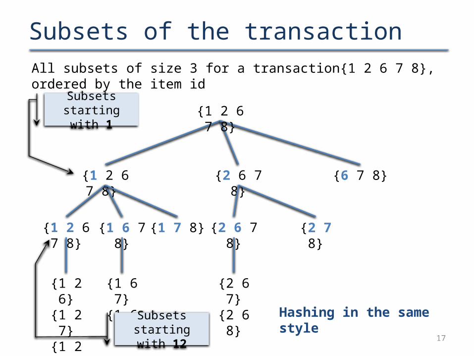
{1 6 7}{1 6 8}
{1 2 6}{1 2 7}{1 2 8}
{1 2 6 7 8}
{6 7 8}{1 2 6 7 8} {2 6 7 8}
{1 2 6 7 8} {1 6 7 8} {1 7 8} {2 6 7 8} {2 7 8}
{2 6 7}{2 6 8}
All subsets of size 3 for a transaction{1 2 6 7 8}, ordered by the item id
Subsets starting with 1
Subsets starting with 12
Hashing in the same style
18
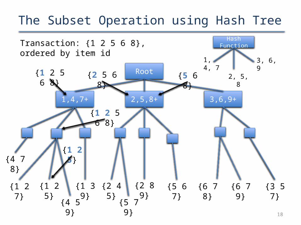
The Subset Operation using Hash TreeTransaction: {1 2 5 6 8}, ordered by item id Hash Function
1, 4, 7
2, 5, 8
3, 6, 9
Root
1,4,7+ 2,5,8+ 3,6,9+
{1 2 5}{1 2 7} {1 3 9} {2 4 5} {2 8 9} {3 5 7}
{4 5 9}
{4 7 8}
{5 6 7}
{5 7 9}
{6 7 8} {6 7 9}
{1 2 5 6 8} {2 5 6 8} {5 6 8}
{1 2 5 6 8}
{1 2 5}

19
Where are we now? Computed frequent itemsets, i.e. the itemsets with required
support minsup Each frequent k-itemset X gives rise to several association
rules Ignoring X ϕ and ϕ X, 2k – 2 rules Rules generated from different itemsets are also different The rules need to be checked for minimum confidence All these rules already satisfy the support condition
How many?
20
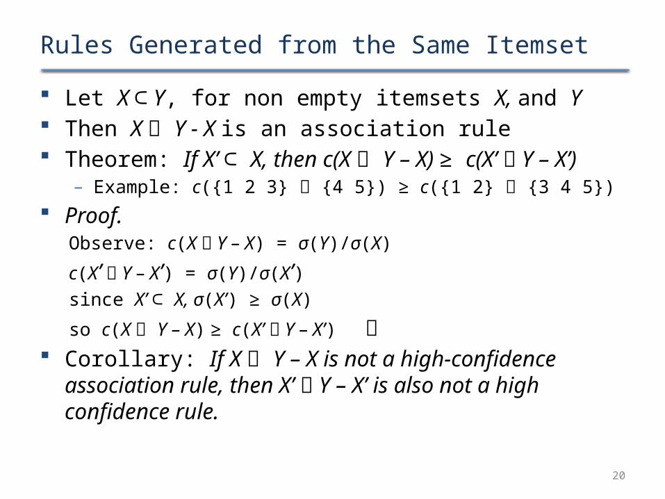
Rules Generated from the Same Itemset Let X ⊂ Y, for non empty itemsets X, and Y Then X Y - X is an association rule Theorem: If X’ ⊂ X, then c(X Y – X) ≥ c(X’ Y – X’)
– Example: c({1 2 3} {4 5}) ≥ c({1 2} {3 4 5})
Proof. Observe: c(X Y – X) = σ(Y)/σ(X)
c(X’ Y – X’) = σ(Y)/σ(X’)since X’ ⊂ X, σ(X’) ≥ σ(X)
so c(X Y – X) ≥ c(X’ Y – X’)
Corollary: If X Y – X is not a high-confidence association rule, then X’ Y – X’ is also not a high confidence rule.

21
Level-wise Approach for Rule Generation
Frequent itemset: {1 2 3 4}
{1 3 4} {2} {2 3 4} {1}{1 2 4} {3}
{1} {2 3 4}
{1 2} {3 4}
{1 2 3} {4}
{1 3} {2 4} {1 4} {2 3} {2 3} {1 4} {2 4} {1 3} {3 4} {1 2}
{2} {1 3 4} {3} {1 2 4} {4} {1 2 3}
{1 2 3 4} {}
Suppose {1 2 4} {3} fails the confidence bar The whole tree under {1 2 4} {3} can be discarded

Maximal Frequent itemsetsMaximal frequent itemset: an itemset, for which none of its immediate supersets are frequent
22
{3} {4}{2}
{1 2 3}
{1 2}
{1}
{1 3} {1 4} {2 3} {2 4} {3 4}
{1 2 4} {1 3 4} {2 3 4}
{}
{1 2 3 4}
Maximal Frequent itemsetsMaximal frequent itemset: an itemset, for which none of its immediate supersets are frequent
23
{3} {4}{2}
{1 2 3}
{1 2}
{1}
{1 3} {1 4} {2 3} {2 4} {3 4}
{1 2 4} {1 3 4} {2 3 4}
{}
{1 2 3 4}
Not frequent
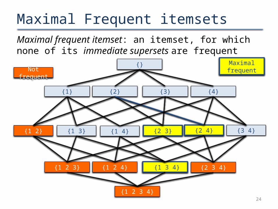
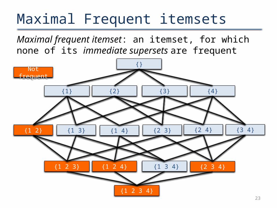
Maximal Frequent itemsetsMaximal frequent itemset: an itemset, for which none of its immediate supersets are frequent
24
{3} {4}{2}
{1 2 3}
{1 2}
{1}
{1 3} {1 4} {2 3} {2 4} {3 4}
{1 2 4} {1 3 4} {2 3 4}
{}
{1 2 3 4}
Not frequent
Maximal frequent

Maximal Frequent itemsetsAll frequent itemsets are subsets of one of the maximal frequent itemsets.
25
{3} {4}{2}
{1 2 3}
{1 2}
{1}
{1 3} {1 4} {2 3} {2 4} {3 4}
{1 2 4} {1 3 4} {2 3 4}
{}
{1 2 3 4}
Not frequent
Maximal frequent
26
Maximal Frequent Itemsets Valuable compact representation of the frequent
itemsets
But
Do not contain the support information of the subsets– Says all supersets have lesser support, but does not say if
any subset also has the same support

27
Closed Frequent Itemsets Closed itemset: an itemset X for
which none of its immediate supersets has exactly the same support count as X – If X is not closed, at least one of
its immediate supersets have the same support as the support of X
Closed frequent itemset: an itemset which is closed and frequent (support ≥ minsup)
Support for non-closed frequent itemsets can be determined from the support information of the closed frequent itemsets
Frequent itemsets
Closed frequent itemsets
Maximal frequent itemsets
28
Evaluation of Association Rules Even from a small dataset a very large number of
rules can be generated– For example, as support and confidence conditions are
relaxed, number of rules explode
Interestingness measure for patterns / rules is required
Objective interestingness measure: a measure that uses statistics derived from the data– Support, confidence, correlation, … – Domain independent– Requires minimal human involvement
29
Subjective Measure of Interestingness The rule {Salami} {Bread} is not so interesting because it is
obvious! Rules such as{Salami} {Dish washer detergent}, {Salami}
{Diper}, etc are less obvious Subjectively more interesting for marketing experts
– Non-trivial cross sell
Methods for subjective measurement– Visualization aided: human in the loop– Template-based: constrains are provided for rules– Filter obvious and non-actionable rules
?
30
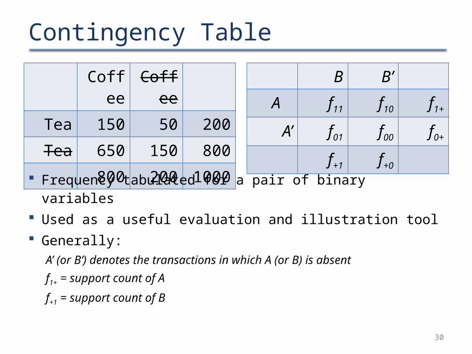
Contingency TableCoffee Coffee
Tea 150 50 200Tea 650 150 800
800 200 1000
B B’A f11 f10 f1+
A’ f01 f00 f0+
f+1 f+0
Frequency tabulated for a pair of binary variables Used as a useful evaluation and illustration tool Generally:
A’ (or B’) denotes the transactions in which A (or B) is absentf1+ = support count of A
f+1 = support count of B
31
Limitations of Support & Confidence Tuning the support threshold is tricky Low threshold – Too many rules generated! High threshold – Potentially interesting patterns may
fall below the support threshold
32
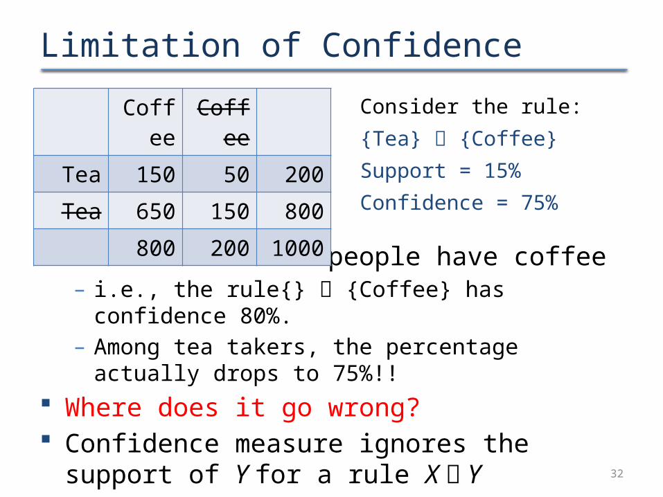
Limitation of Confidence
But: Overall 80% people have coffee– i.e., the rule{} {Coffee} has confidence 80%. – Among tea takers, the percentage actually drops to 75%!!
Where does it go wrong? Confidence measure ignores the support of Y for a
rule X Y
Coffee CoffeeTea 150 50 200Tea 650 150 800
800 200 1000
Consider the rule:{Tea} {Coffee}Support = 15%Confidence = 75%
33
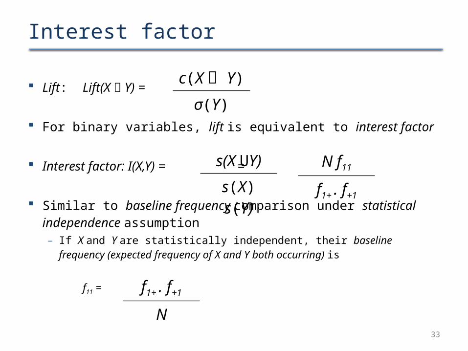
Interest factor
Lift: Lift(X Y) =
For binary variables, lift is equivalent to interest factor
Interest factor: I(X,Y) = =
Similar to baseline frequency comparison under statistical independence assumption– If X and Y are statistically independent, their baseline frequency
(expected frequency of X and Y both occurring) is
f11 =
c(X Y)
σ(Y)
s(X UY)
s(X) s(Y)
N f11
f1+ . f+1
f1+ . f+1
N

34
Interest factor Intuitively
I(X,Y) = 1, if X and Y are independent
> 1, if X and Y have a positive correlation
< 1, if X and Y have a negative correlation
Verify for the tea – coffee example
I(Tea, Coffee)
= 0.15 / (0.2 × 0.8)
= 0.94
Coffee CoffeeTea 150 50 200Tea 650 150 800
800 200 1000
I =N f11
f1+ . f+1
35
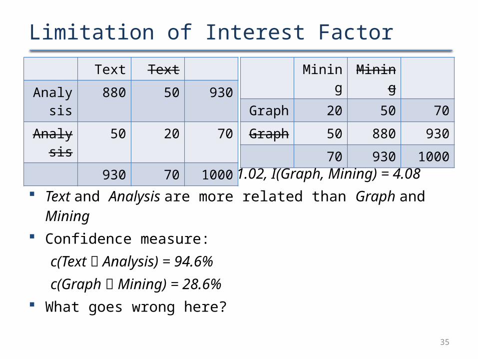
Limitation of Interest Factor
Observe: I(Text, Analysis) = 1.02, I(Graph, Mining) = 4.08 Text and Analysis are more related than Graph and Mining Confidence measure:
c(Text Analysis) = 94.6%
c(Graph Mining) = 28.6% What goes wrong here?
Text TextAnalysis 880 50 930Analysis 50 20 70
930 70 1000
Mining MiningGraph 20 50 70Graph 50 880 930
70 930 1000
36
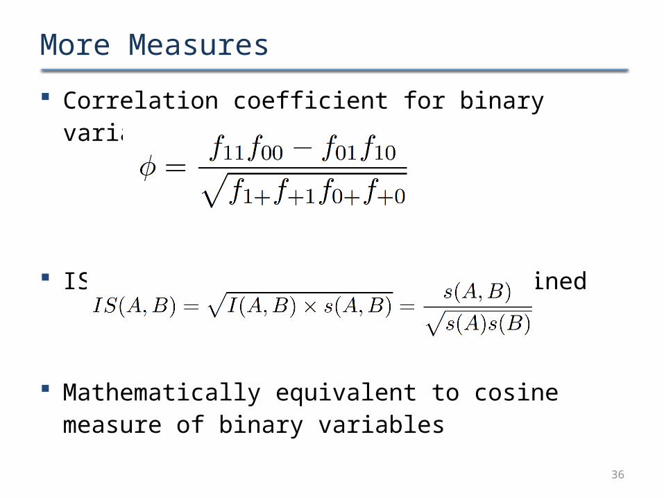
More Measures Correlation coefficient for binary variables:
IS Measure: I and S measures combined
Mathematically equivalent to cosine measure of binary variables
37
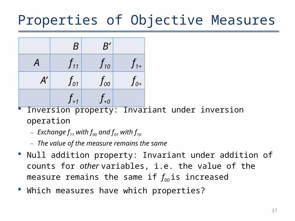
Properties of Objective MeasuresB B’
A f11 f10 f1+
A’ f01 f00 f0+
f+1 f+0
Inversion property: Invariant under inversion operation– Exchange f11 with f00 and f01 with f10
– The value of the measure remains the same
Null addition property: Invariant under addition of counts for other variables, i.e. the value of the measure remains the same if f00 is increased
Which measures have which properties?

38
References Rakesh Agrawal and Ramakrishnan Srikant
Fast Algorithms for Mining Association Rules
VLDB 1994 Introduction to Data Mining, by Tan, Steinbach, Kumar
– The webpage: http://www-users.cs.umn.edu/~kumar/dmbook/index.php
– Chapter 6 is available online: http://www-users.cs.umn.edu/~kumar/dmbook/ch6.pdf


