

Bankruptcy prediction: the case of Japanese listedcompanies
Ming Xu Æ Chu Zhang
Published online: 26 July 2008
� Springer Science+Business Media, LLC 2008
Abstract This paper investigates if bankruptcy of Japanese listed companies can
be predicted using data from 1992 to 2005. We find that the traditional measures,
such as Altman’s (J Finance 23:589–609, 1968) Z-score, Ohlson’s (J Accounting
Res 18:109–131, 1980) O-score and the option pricing theory-based distance-to-
default, previously developed for the U.S. market, are also individually useful for
the Japanese market. Moreover, the predictive power is substantially enhanced
when these measures are combined. Based on the unique Japanese institutional
features of main banks and business groups (known as Keiretsu), we construct a new
measure that incorporates bank dependence and Keiretsu dependence. The new
measure further improves the ability to predict bankruptcy of Japanese listed
companies.
Keywords Bankruptcy risk measure � Accounting information � Option
pricing theory � Japanese listed companies � Bank dependence � Keiretsu
JEL Classifications G15 � G33
1 Introduction
When a company falls into bankruptcy, its stakeholders lose some or all the value
they invested in the company. From an investor’s point of view, it is important to
M. Xu (&)
School of Accounting and Finance, The Hong Kong Polytechnic University, Kowloon,
Hong Kong, China
e-mail: [email protected]
C. Zhang
Department of Finance, The Hong Kong University of Science and Technology, Kowloon,
Hong Kong, China
123
Rev Account Stud (2009) 14:534–558
DOI 10.1007/s11142-008-9080-5

assess a firm’s likelihood of bankruptcy so that the bankruptcy risk can be
appropriately compensated in expected returns. Academic researchers and practi-
tioners have developed various models to estimate bankruptcy risk. These models
have been applied mostly to U.S. companies. The current debate in the literature
about the performance of the models centers on two issues. The first issue is related
to the usefulness of accounting variables versus market variables in predicting
bankruptcy. The second issue is about ad hoc statistical models versus option
pricing theory-based models.
The early bankruptcy prediction models are based on accounting variables.
Examples include Beaver (1966, 1968); Altman (1968);1 Altman et al. (1977);
Ohlson (1980); and Zmijewski (1984). The variables used to give an early warning
of bankruptcy are mostly traditional accounting ratios from financial statements.
Shumway (2001), however, finds that half of the accounting variables used by
Altman (1968) and Zmijewski (1984) are statistically unrelated to bankruptcy
probability. Instead, he argues, some market variables such as firm size, past stock
returns, and idiosyncratic returns variability are all strongly related to bankruptcy
risk. By combining two accounting ratios and three market variables together,
Shumway’s hazard model outperforms the previous models. Chava and Jarrow
(2004) support Shumway’s (2001) model by showing that accounting variables add
little predictive power when market variables are already included in the bankruptcy
model. On the other hand, a study by Beaver et al. (2005) using a similar model
with a longer time period finds that the ability of accounting ratios to predict
bankruptcy remains. Their findings indicate that the market variables complement
accounting variables and that the use of market variables causes only a slight
reduction of predictive power of the accounting variables in certain subperiods.
While statistical models have been widely used in practice, option pricing theory-
based models have gained in popularity. With the option pricing theory-based
models, both the predictive variables and the functional form of the predictive
relationship are rigorously derived, unlike the statistical models in which both are
based on intuition only. Several recent papers have used the standard Black–Scholes
model to estimate bankruptcy risk. Examples include Crosbie and Bohn (2002);
Vassalou and Xing (2004); and Hillegeist et al. (2004). As reported by Vassalou and
Xing (2004) and Hillegeist et al. (2004), the option pricing theory-based bankruptcy
risk measures outperform those based on traditional statistical models.
In this paper, we examine the possibility of predicting the bankruptcy of Japanese
listed companies using accounting variables, option pricing theory-based variables,
and other variables unique to the Japanese economy. The Japanese market merits
this analysis for two reasons. First, most academic research on predicting
bankruptcy has been conducted on U.S. companies. Whether or not models
developed for U.S. companies also work outside the U.S. is a question that has not
been previously answered. Japan is a natural choice because the Japanese economy
is comparable with that of the United States in many aspects. The Japanese stock
market in terms of market capitalization was the second largest in the world during
1 Altman’s (1968) model includes one market-based measure: the ratio of the market value of equity to
the book value of total liabilities.
Bankruptcy prediction 535
123

the sample period we study, next to that of the United States. By using a previously
untested data set, we gain understanding of how bankruptcy prediction models
might work outside the U.S. market. Since the time period of the Japanese data set is
shorter than that of the U.S. data set and the sample size of the Japanese data set is
smaller than that of the United States, we do not expect to resolve the debates in the
literature about what kind of variables are more useful in predicting bankruptcy and
what type of model is more accurate. Nevertheless, evidence from the Japanese data
should illuminate unresolved issues arising from the U.S. studies. Second, while
Japan’s financial market is well developed, like the one in the United States, it does
have its own unique characteristics. One of the important features of the corporate
structure in Japan is the so-called main bank system, in which each company is
associated with a main commercial bank. There are several large business groups
centered on large banks known as horizontal Keiretsu. Whether a company belongs
to one of the Keiretsu groups and how close it is to its main bank should have
important bearing on how likely the company is to go bankrupt in the short run.
Companies having close ties with their banks and other companies within a Keiretsu
tend to get help when they face financial difficulties. Therefore these companies
tend to have lower bankruptcy risk, other things being equal. The Japanese setting is
ideal for examining the role that institutional arrangements may play in predicting
bankruptcy beyond variables from accounting statements and financial markets.
We address two questions. First, do models developed for predicting the
bankruptcy of U.S. companies remain valid in principle for predicting the
bankruptcy of Japanese companies? Second, do corporate structure variables affect
the probability of bankruptcy? For the first question, we simply borrow the original
models from the existing literature with slight modification. We estimate a version
of Altman’s Z-score, Ohlson’s O-score and the option pricing theory-based measure
of the bankruptcy risk for Japanese listed companies. For the second question, we
construct two variables that measure how closely a company is related to its main
bank and the extent to which it belongs to a Keiretsu. One variable is the proportion
of the company’s stock held by its banks, which is a proxy for the dependence of the
company on its banks. The other variable is a rating of the company’s inclination to
be in a Keiretsu, which is based on various criteria explained in the main text. We
add these two variables to the accounting and market based variables and test how
they contribute to bankruptcy prediction.
Our results show that the models based on accounting information and stock
market information remain valid for Japanese listed companies. While not all the
variables in these models are significant and the estimated parameters differ from
those estimated from the data for U.S. companies, these models capture the fact that
bankruptcy is a lengthy process and that the deterioration of a company’s financial
status is reflected in its financial statements and stock prices. We also find that these
models are non-exhaustive and non-exclusive. Combining some of the variables in
all three models generates a model that has more predictive power than each of the
three models does alone. The two new variables, bank dependence and Keiretsu
dependence, which capture the main feature of the corporate structure in Japan, are
found to be useful in predicting bankruptcy of Japanese listed companies. They
contribute to the prediction model to a certain extent.
536 M. Xu, C. Zhang
123
The remainder of this paper is organized as follows. Section 2 reviews the
existing literature on bankruptcy prediction models and provides the details of the
methodology used to estimate the models. Section 3 describes the institutional
background of Japanese firms and the two new variables that indicate bank
dependence and Keiretsu dependence. Section 4 presents data sources and simple
statistics of the variables used in various models. Section 5 reports the results of the
estimated bankruptcy prediction models and compares the performance of these
models. The last section summarizes the paper.
2 Existing models of bankruptcy prediction
Statistical models using accounting data to predict bankruptcy abound. A popular
method used to estimate the likelihood of bankruptcy is multiple discriminant
analysis. Altman (1968) uses the method to examine a sample of 66 manufacturing
companies, half of which filed bankruptcy petitions under Chapter X of the U.S.
National Bankruptcy Act during the period from 1946 to 1965. Altman considers 22
financial ratios, of which five are found to be useful for predicting bankruptcy. The
estimated model takes the form:
Zit ¼ 1:2V1it þ 1:4V2it þ 3:3V3it þ 0:6V4it þ 0:999V5it; ð1Þ
where t is a year, i is a company, and Zit is a score to indicate the probability for
company i to survive in year t + 1, and V1 = Working capital/Total assets;
V2 = Retained earnings/Total assets; V3 = Earnings before interest and taxes/Total
assets; V4 = Market value of equity/Book value of total liabilities; V5 = Sales/Total
assets.
The fitted value of Zit is known as the Z-score for company i in year t. The higher
the Z-score, the higher the chance of survival. Overall, these five accounting ratios
capture the company’s characteristics such as liquidity, profitability, productivity,
solvency and sales-generating ability.
Ohlson (1980) uses conditional logit models to predict bankruptcy. The best
known model is his Model 1, which identifies four basic factors that affect the
probability of bankruptcy within 1 year: (1) company size; (2) financial structure;
(3) performance; and (4) current liquidity. These four factors are represented by
nine accounting variables. Using data from the period of 1970–1976 with 105
bankrupt companies and 2058 non-bankrupt companies, his Model 1 is estimated as:
Oit ¼� 1:32� 0:407W1it þ 6:03W2it � 1:43W3it þ 0:076W4it
� 1:72W5it � 2:37W6it � 1:83W7it þ 0:285W8it � 0:521W9it;ð2Þ
where the observation on Oit is one if company i goes bankrupt during the next year
and zero otherwise, and W1 = log(Total assets/GNP price-level index); W2 = Total
liabilities/Total assets; W3 = Working capital/Total assets; W4 = Current liabili-
ties/Current assets; W5 = One if total liabilities exceeds total assets, zero otherwise;
W6 = Net income/Total assets; W7 = Funds from operations/Total liabilities;
W8 = One if net income was negative for the last 2 years, zero otherwise;
W9 = (Net incomet - Net incomet-1)/(|Net incomet| + |Net incomet-1|).
Bankruptcy prediction 537
123

The fitted value of Oit is known as the O-score for company i in year t. The
greater the O-score, the higher its bankruptcy risk.
Both Altman’s model and Ohlson’s model continued to work well in the 1980s
and the 1990s, as shown by Altman (1993), Begley et al. (1996) and Dichev (1998).
In the current paper, we adopt the same sets of variables to determine the
bankruptcy risk for Japanese listed companies, by using a hazard model to estimate
the coefficients:
~Zit ¼ Uða0 þ a1V1it þ a2V2it þ a3V3it þ a4V4it þ a5V5itÞ; ð3Þ
Oit ¼Uðb0 þ b1W1it þ b2W2it þ b3W3it þ b4W4it þ b5W5it þ b6W6it
þ b7W7it þ b8W8it þ b9W9itÞ;ð4Þ
where the observations of ~Zit and Oit are one if company i goes bankrupt within a
year and zero if not, U is the cumulative standard normal distribution function, and
the fitted values of ~Zit and Oit are the models’ predictions of the probability of
bankruptcy within a year. The independent variables are the same as those in
Altman (1968) and Ohlson (1980). Note that what we call the Z-score and O-score
refer to the accounting variables used in the original work. The method we use to
estimate the model follows Shumway (2001). As shown by Shumway (2001), the
hazard model is theoretically preferable to the static models used previously because
it uses all available information to produce bankruptcy probability estimates for all
firms at each point in time and avoids the selection biases inherent in static models.
To compare Altman’s model with Ohlson’s model and other models to be discussed
later, we define the fitted value of ~Zit as the probability of bankruptcy, instead of a
measure of survival.
While accounting information is useful, it tends to look backwards. There is
information that may not be contained in accounting statements but reflected in the
price of stocks if the companies are listed and frequently traded. The information in
stock prices tends to be more forward looking. In the recent literature, a new
methodology for bankruptcy prediction has emerged that is based on the option pricing
theory. As have been well articulated, the equity of a company with a simple capital
structure can be viewed as a call option written on its assets with its debt as the strike
price. Therefore, bankruptcy can be interpreted as the call finishing out of money at the
maturity of the debt, whose probability can be calculated using standard option pricing
models developed by Black and Scholes (1973) and Merton (1973, 1974). Vassalou
and Xing (2004) compute the default likelihood indicator (DLI) to measure bankruptcy
probability in such a framework. Hillegeist et al. (2004) use a similar approach to
compute bankruptcy probability. The difference between Vassalou and Xing (2004)
and Hillegeist et al. (2004) is a technical one about adjustments for dividends. Since
the difference is small, we follow Vassalou and Xing (2004) in the rest of the
discussion. In the Black–Scholes–Merton setting, the market value of a company’s
underlying assets follows a geometric Brownian motion of the form:
dVit ¼ liVitdt þ riVitdWit; ð5Þ
where V is the value of company i’s total assets, l is its instantaneous drift, r is its
instantaneous volatility, and W is a standard Wiener process whose change
538 M. Xu, C. Zhang
123
represents unpredictable shocks to the asset value. Suppose that the firm has a single
debt, X, to be paid at t + T. Then, the bankruptcy probability, defined as the
probability for the company’s assets to be less than the book value of the company’s
liabilities at t + T, is
DLIit ¼ PrðVi;tþT �XitjVitÞ ¼ PrðlnðVi;tþTÞ� lnðXtÞjVitÞ
¼ U �InðVit=XitÞ þ ðli � 1
2r2
i ÞTri
ffiffiffiffi
Tp
� �
� Uð�DDitÞ;ð6Þ
where U is the cumulative density function of the standard normal distribution. The
quantity DD is known as the distance-to-default measure. It measures the distance
between the current value of assets and the debt amount in terms of the volatility,
that is, the standard deviation of the growth rate, of the assets.2 Apart from the stock
price, asset value volatility also enters the calculation of the default probability. This
is an additional advantage of using the option pricing theory-based model to
estimate bankruptcy probability. Note that (6) follows from (5) without dependence
on the option pricing theory. However, since the market value of assets and its drift
and volatility are not directly observed, the option pricing theory is conducive to
estimating the asset process from the observed stock price and its volatility.
Vassalou and Xing (2004) use an iterative procedure to estimate V and r first and
then to calculate DLI. Since typically a company will have a more complicated
capital structure than the model assumes, for convenience, T is chosen to be 1 year
and Xt is chosen to be all the short-term debt (with maturities less than 1 year) plus
half of the long-term debt (with maturities greater than 1 year). For companies that
have no debt, DD is set at five which corresponds to a DLI of virtually zero.3
We use a hazard model to estimate the following bankruptcy measure, named the
D-score:4
Dit ¼ Uðc0 þ c1DDitÞ: ð7ÞThe DLI is a special case when c0 = 0 and c1 = -1. The added flexibility given
by the free parameters can improve the predictive power of the option pricing
theory-based measures.
The accounting variable-based models and option pricing theory-based models
have strengths and weaknesses. Accounting variable-based models have the
advantage of the abundance of information regarding all aspects of a company’s
2 Despite its name, DD can take negative values. It is possible for the asset value to be less than the
amount of debt before the debt is due.3 There are further developments along the line. Brockman and Turtle (2003), Leland (2004), and
Charitou and Trigeorgis (2004) deviate from the standard option pricing model by incorporating some
more realistic assumptions about default and bankruptcy. Bharath and Shumway (2005) examine the
accuracy and the contribution of the theory-based models, and they conclude that the theory-based models
have slightly better out-of-sample performance than statistical models have. Campbell et al. (2007)
present evidence that bankruptcy risk cannot be adequately summarized by a theory-based measure, while
Duffie et al. (2007) confirm that theory-based measures can predict bankruptcy.4 Our choice of the default boundaries follows those in Crosbie and Bohn (2002); Vassalou and Xing
(2004); and Hillegeist et al. (2004). The results remain qualitatively the same with different default
boundaries.
Bankruptcy prediction 539
123

past activities, such as the amount of debt, earnings, and sales. But they tend to look
backwards, and the models are mostly empirically determined. The option pricing
theory-based models are theoretically rigorous and forward looking, but they are
weak in their reliance on perhaps oversimplified assumptions about the capital
structure of the companies and the restrictive assumptions about the stochastic
processes governing the asset values. We, therefore, consider a combined model that
comprises various ingredients of both types of models. Obviously, some of the
variables used in the Z-score and the O-score are highly correlated and may proxy
for similar company characteristics. We use the stepwise approach to remove
insignificant variables from the regression model. Specifically, the variables are
entered into and removed from the model in such a way that each forward selection
step is followed by one or more backward elimination steps. The selection process
terminates if no further variable can be added to the model, or if the variable just
entered into the model is the only variable removed in the subsequent backward
elimination. Eventually, we arrive at the following model:
Cit ¼ Uðd0 þ d1V5it þ d2W4it þ d3W8it þ d4DDitÞ; ð8Þ
where the definitions of variables are the same as before. This C-score contains
accounting information on current sales, liabilities, liquidity, earnings, and the
market information about future profitability and asset value volatility. It
synthesizes the accounting variable-based models and the option pricing theory-
based models.
3 Japanese corporate structure and bankruptcy prediction
The Japanese economy has its own unique structure that necessitates fine-tuning of
the bankruptcy risk measures. To explain how we include corporate structure
variables in a new bankruptcy predicting model, we first briefly review the evolution
over time of the relationship of Japanese companies with their banks.
Unlike their U.S. counterparts, Japanese companies rely more on banks, instead
of financial markets, for financing. It has been documented extensively that equity
holdings in companies by their main banks and other financial institutions are
substantial in Japan. This is not seen in United States for regulatory reasons. Until
the late 1980s, a Japanese company’s access to credit was mostly dictated by its
affiliation to an economic group built around its main bank. Under the main bank
system, main banks had privileged knowledge of companies’ prospects and
strengths, so they were in a good position to monitor the companies’ performance.
This was especially so when bank officers served on the companies’ boards. Even if
some companies fell into distress, the main banks would try to rescue them.
Typically, the company’s main bank would ease its own credit terms to the
distressed company, pay off other bank creditors, and put pressure on the suppliers
of the company to continue to do business with the distressed company. This
practice resulted in relatively few exchange-listed companies going bankrupt before
the end of the 1980s.
540 M. Xu, C. Zhang
123
The financial liberalization in the 1980s in Japan allowed large companies to
reduce their dependence on bank loans and to obtain cheaper financing through
financial markets. This prompted the banks to look for new customers, mainly
among smaller companies and nonmanufacturing companies. In particular, much
credit was extended to the construction and real estate sectors through banks’
nonbank subsidiaries. The banks usually relied on pledges of collateral rather than
on careful monitoring of these new clients. Thus, when a bubble in the stock market
and the property market burst in 1990, banks had less incentive to provide
significant support to those clients that were difficult to monitor or control.
Nevertheless, bankruptcies among large companies were still contained during most
of the 1990s. Although banks were no longer so willing to rescue distressed
companies, they were still reluctant to force companies into bankruptcy. Loan
syndication made every bank vulnerable to other banks’ actions, so banks preferred
to roll over their loans to distressed companies without forcing them into
bankruptcy. Therefore, the balance sheets of banks were weakened by many
nonperforming loans. In late 1997, three large financial institutions failed.
According to Nakamura (2006), in 1998, the Japanese government tightened its
regulatory standards and ordered banks to reduce the holdings in their client
companies and improve their financial performance. Only then did banks start to
reassess their strategies and curtail credit. Gradually, banks came to prefer solving
financial problems via transparent legal procedures to save time, costs and expenses.
As a result, the number of bankruptcies started to increase.
An illustration of the changing landscape of the Japanese main bank system is
Sogo, a well-known department store chain. The Industrial Bank of Japan (IBJ) was
its largest lender, providing 21.7% of Sogo’s loans and holding 4.99% of its shares
in 1996. One of the vice presidents of Sogo was an ex-IBJ banker. In the late 1990s,
Sogo fell into financial trouble and faced pressure from many of its creditors. At that
time, IBJ intervened and prevented Sogo from going bankrupt. By early 2000, IBJ
realized that it could not support Sogo by itself any more. A rescue attempt was
made by IBJ when it asked all the other major lenders to Sogo to ease their terms.
The attempt failed, however, and Sogo was forced to apply for a court-supervised
restructuring. The story of Sogo’s bankruptcy is documented by Hoshi and Kashyap
(2001), among others.
In addition to the main bank system, the Keiretsu system is also unique to the
corporate structure in Japan. A Keiretsu is a large business group surrounding a few
large financial institutions and manufacturing companies collectively known as the
nucleus. According to Flath (2001), there were eight Keiretsu groups in the 1990:
Mitsubishi, Mitsui, Sumitomo, Fuyo, DKB, Sanwa, IBJ and Tokai. The members of
a Keiretsu are connected through crossholding of shares, mutual appointment of
directors, and intra-group financing. Obviously, such a group structure gives its
members an advantage in acquiring loans with favorable terms from financial
institutions within the group, especially from the main bank. In addition, long-term
relationships from cross-shareholding help maintain greater commitments among
Keiretsu members and help cement Keiretsu ties. For this reason, a company’s
bankruptcy risk is reduced if it is affiliated with a specific Keiretsu. Hoshi et al.
(1990) find that Keiretsu members invest and sell more after the onset of distress
Bankruptcy prediction 541
123

than do nonmember companies. Suzuki and Wright (1985) provide statistical
evidence on the role of Keiretsu financing in reducing the costs of financial distress.
With a model that predicts whether a troubled company would file for bankruptcy or
would be given concessions by its creditors, they find that Keiretsu members are
more likely to be given concessions on interest or principal payments. It should be
noted that Keiretsu dependence and bank dependence are two different concepts,
although the nucleus of a Keiretsu is a bank. For one thing, most listed companies
are not Keiretsu members. Sogo, for example, is not a Keiretsu member.
Like the main bank system, Keiretsu also experienced serious challenges after the
bubbles in the stock market and the property market burst in the early 1990s. The
group system continued to weaken as cross-shareholding gradually decreased. In
2001, there were significant changes in the Keiretsu. The original eight Keiretsu
were replaced by four new Megabank Groups (Mitsubishi Tokyo Financial Group
Inc., Sumitomo Mitsui Banking Corp., UFJ Holdings Inc., and Mizuho Holdings
Inc.). In the new Keiretsu system, cross-shareholding and intra- and inter-group
consolidation are no longer characteristics, and the nucleus is not strong enough to
exert controlling power over its members. The weakening of both the main-bank
system and the Keiretsu system resulted in more bankruptcy cases in Japan in the
2000s.
The potential effect of the main bank/Keiretsu systems on bankruptcy risk has
been discussed in literature. Shread (1989, 1994) uses 42 cases of main bank rescues
in Japan from the mid-1960s to the late 1980s and finds that the main bank system
efficiently reduces the problems of firms in distress. Miwa and Mark Ramseyer
(2005) investigate troubled firms in two particular years (1978 and 1984) and find
no strong evidence that the firms with main bank affiliations are more likely to
receive assistance from their main bank than are firms without such an affiliation.
Both studies examine the period before the burst of stock market bubble in 1990–
1992 when bankruptcy was rare.
In this paper, we test whether the implicit rescuing contracts between companies
and their main banks/Keiretsu exist in a more recent period from 1992 to 2005. We
use two variables that proxy for bank dependence and Keiretsu dependence. For the
former, we use the fraction of a listed company’s stock directly owned by financial
institutions including banks, insurance companies, securities companies, and other
financial companies. This variable speaks for itself and needs no further
explanation. For the latter, we adopt the rating given by Brown & Company Ltd.
in its biannual publication Industrial Groupings in Japan. The dependence on the
Keiretsu varies widely across the different companies. The following factors are
taken into account in arriving at the degree of inclination towards membership in a
specific group: the characteristics and historical background of the group or the
company; sources and amounts of bank loans; board directors sent by or sent to the
nucleus or other group companies; the company’s attitude towards the group; and
the company’s connections with other group or nongroup companies. As such, a
company’s inclination to be a member of a Keiretsu group is rated on a scale of zero
to four asterisks. Companies rated with four asterisks are nucleus group companies.
The companies with strong inclinations towards membership in a Keiretsu are rated
with three asterisks. Companies rated with two asterisks are inclined towards and
542 M. Xu, C. Zhang
123
connected with a Keiretsu, but the links are not particularly strong. The companies
with weak inclination to be members in a Keiretsu are rated with one asterisk.
Companies unrelated to any Keiretsu group receive a rating of zero asterisks. The
model for the new bankruptcy risk measure, the X-score, is as follows:
Xit ¼ Uðe0 þ e1V5it þ e2W4it þ e3W8it þ e4DDit þ e5U1it þ e6U2itÞ; ð9Þ
where U1 is the ownership by financial institutions in year t, U2 is the inclination
towards a membership in a Keiretsu (0–4) in year t, and the other explanatory
variables are defined as above.
4 Data
The data used in this study are taken from the PACAP Japanese database and
Datastream Inc. We include all the Japanese listed companies from 1992 to 2005,
except for financial service companies (banks, insurance and securities companies).
Companies in these financial industries are structurally different and have a different
bankruptcy environment. While Japan has nine stock exchanges (the Tokyo, Osaka,
Nagoya, Kyoto, Hiroshima, Fukuoka, Niigata, Sapporo and JASDAQ exchanges),
the market is dominated by the Tokyo Stock Exchange (TSE) with around 90% of
the country’s total market capitalization. Most Japanese capital market studies focus
on the TSE. The TSE is divided into a main section and a secondary section,
referred to as sections 1 and 2, respectively. Typically, smaller companies are listed
on the second section, and they may move to the first section when they satisfy the
standards set by the exchange. Data on the companies listed on the TSE are
retrieved from the PACAP Japanese database. Most of the companies listed on the
TSE are large companies that conform to the listing requirements. Generally, small
companies tend to have higher bankruptcy risk. To avoid distorting the analysis, we
include the companies listed on the other stock exchanges as well, as long as the
required accounting variables are available. Data on those companies come from
Datastream Inc. As shown in Table 1, there are 3,510 listed companies in the final
sample, with 2,055 companies listed on the TSE. Most of the sample companies are
in the manufacturing industry.
We examine performance-related delistings. The reasons given for this kind of
delisting are formally classified as liquidation, rehabilitation, reorganization and
failure to meet the listing conditions.5 We regard all these cases as bankruptcy.
Although the data start from 1975, no listed nonfinancial companies went bankrupt
before 1993. Since standard models in the literature predict bankruptcy within
1 year, we confine our analysis to the period from 1992 to 2005. During the sample
period, the number of exchange-listed companies going bankrupt is relatively small,
5 There were mainly three types of bankruptcy filings available to large companies in Japan: the Civil
Rehabilitation Law, the Corporate Reorganization Law and the Liquidation Law. The Liquidation Law is
equivalent to Chapter 7 of the U.S. Bankruptcy Code, whereas the Civil Rehabilitation Law and the
Corporate Reorganization Law are roughly equivalent to Chapter 11 of the U.S. Bankruptcy Code. Xu
(2004) found that bankrupt Japanese companies preferred rehabilitation or reorganization to liquidation,
which is similar to the U.S. evidence in Bris et al. (2006).
Bankruptcy prediction 543
123
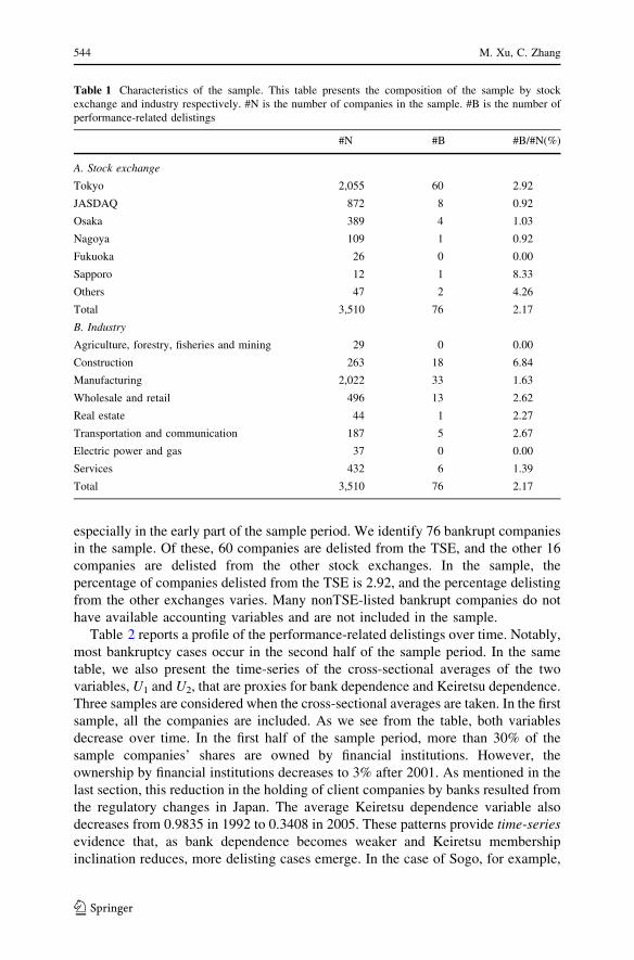
especially in the early part of the sample period. We identify 76 bankrupt companies
in the sample. Of these, 60 companies are delisted from the TSE, and the other 16
companies are delisted from the other stock exchanges. In the sample, the
percentage of companies delisted from the TSE is 2.92, and the percentage delisting
from the other exchanges varies. Many nonTSE-listed bankrupt companies do not
have available accounting variables and are not included in the sample.
Table 2 reports a profile of the performance-related delistings over time. Notably,
most bankruptcy cases occur in the second half of the sample period. In the same
table, we also present the time-series of the cross-sectional averages of the two
variables, U1 and U2, that are proxies for bank dependence and Keiretsu dependence.
Three samples are considered when the cross-sectional averages are taken. In the first
sample, all the companies are included. As we see from the table, both variables
decrease over time. In the first half of the sample period, more than 30% of the
sample companies’ shares are owned by financial institutions. However, the
ownership by financial institutions decreases to 3% after 2001. As mentioned in the
last section, this reduction in the holding of client companies by banks resulted from
the regulatory changes in Japan. The average Keiretsu dependence variable also
decreases from 0.9835 in 1992 to 0.3408 in 2005. These patterns provide time-seriesevidence that, as bank dependence becomes weaker and Keiretsu membership
inclination reduces, more delisting cases emerge. In the case of Sogo, for example,
Table 1 Characteristics of the sample. This table presents the composition of the sample by stock
exchange and industry respectively. #N is the number of companies in the sample. #B is the number of
performance-related delistings
#N #B #B/#N(%)
A. Stock exchange
Tokyo 2,055 60 2.92
JASDAQ 872 8 0.92
Osaka 389 4 1.03
Nagoya 109 1 0.92
Fukuoka 26 0 0.00
Sapporo 12 1 8.33
Others 47 2 4.26
Total 3,510 76 2.17
B. Industry
Agriculture, forestry, fisheries and mining 29 0 0.00
Construction 263 18 6.84
Manufacturing 2,022 33 1.63
Wholesale and retail 496 13 2.62
Real estate 44 1 2.27
Transportation and communication 187 5 2.67
Electric power and gas 37 0 0.00
Services 432 6 1.39
Total 3,510 76 2.17
544 M. Xu, C. Zhang
123

the weakening tie to the main bank and other financial institutions is reflected in its
U1. The value of its U1 was 52.44% in 1992. It gradually decreased to 11.43% in
1999 and finally became zero before the company went bankrupt in 2000. Note that
the number of companies in the full sample increases over time. The new companies
tend to be smaller ones with weaker ties with main banks and Keiretsu. One might
wonder if the decline in the average bank dependence and the average Keiretsu
dependence is caused by the inclusion of these new companies in the sample. To
answer that question, we examine cross-sectional averages over two more samples.
One sample, the 1992-sample, includes only companies that existed in 1992. The
number of companies in the sample decreases as some companies are delisted for
either performance-related reasons or other reasons. The other sample, the 1992–
2005-sample, includes only companies that existed during the entire 1992–2005
period. While the numbers in the table show that all the averages follow a decreasing
pattern over time, two observations are worth noting. First, the patterns for bank
dependence are very similar in all three samples. This means that the declining
pattern in bank dependence we see in the full sample is not due to the inclusion of
new companies. Second, Keiretsu dependence declines faster in the full sample than
in the 1992-sample, which in turn is faster than in the 1992–2005-sample. This means
that the decreasing pattern of Keiretsu dependence that we see in the full-sample is
Table 2 Summary report of Japanese performance-related delistings. This table reports the profile of
performance-related delistings over time. #N is the number of companies in the sample. #B is the number
of performance-related delistings. The cross-sectional averages of bank dependence and Keiretsu
dependence are also reported. U1 = Ownership by financial companies; U2 = Inclination towards the
membership in a Keiretsu (taking values from 0 to 4). U1 and U2 are the cross-sectional averages of U1
and U2 for all the companies in the sample; U�1 and U�2 are the cross-sectional averages of U1 and U2 for
the companies that existed in 1992 with a sample size of 1273 in 1992 and 970 in 2005; U��1 and U��2 are
the cross-sectional averages of U1 and U2 for the 970 companies that existed during the entire sample
period from 1992 to 2005
Year #B Full-sample 1992-Sample 1992–2005-Sample
#N U1 U2 U�1 U�2 U��1 U��2
1992 0 1,273 0.3776 0.9835 0.3776 0.9835 0.3819 1.0220
1993 1 1,434 0.3691 0.9766 0.3724 0.9834 0.3744 1.0166
1994 0 1,473 0.3658 0.9697 0.3704 0.9904 0.3725 1.0134
1995 1 1,499 0.3606 0.9652 0.3646 0.9910 0.3677 1.0131
1996 0 1,539 0.3513 0.9529 0.3564 0.9989 0.3595 1.0069
1997 6 1,577 0.3373 0.9370 0.3440 0.9842 0.3454 1.0048
1998 5 1,617 0.2997 0.8603 0.3270 0.9765 0.3271 0.9971
1999 6 1,810 0.2689 0.7979 0.3078 0.9523 0.3080 0.9958
2000 8 2,018 0.2207 0.6627 0.2882 0.9424 0.2914 0.9618
2001 7 2,678 0.1071 0.5463 0.1534 0.8711 0.1551 0.9114
2002 11 2,746 0.0357 0.4632 0.0504 0.8455 0.0507 0.8504
2003 10 2,880 0.0373 0.4230 0.0573 0.8222 0.0583 0.8477
2004 10 3,078 0.0348 0.3937 0.0535 0.8146 0.0543 0.8293
2005 11 3,230 0.0333 0.3408 0.0516 0.7749 0.0516 0.7749
Bankruptcy prediction 545
123

indeed partially due to the inclusion of new companies, although Keiretsu
dependence of existing companies also exhibits significant decline. The difference
in Keiretsu dependence between the 1992-sample and the 1992–2005-sample is also
worth noting. The average Keiretsu dependence is higher for the 1992–2005-sample
than for the 1992-sample, indicating that the companies exiting from the 1992-
sample (either because of performance-related reasons or because of merger and
acquisitions) are those with weaker Keiretsu ties. This is cross-sectional evidence
showing that Keiretsu dependence reduces bankruptcy risk.
Table 3 presents descriptive statistics for the explanatory variables that are used to
estimate the bankruptcy risk measures. We first calculate the time-series average of
the explanatory variables for each Japanese company in the sample. We then report
descriptive statistics for the cross-sectional distribution of the sample companies,
including the mean, standard deviation (Std), and quartiles of the distributions
(minimum, lower quartile, median, upper quartile, and maximum) of the time-series
averages. Since the sample size increases over time, the descriptive statistics
calculated this way are more indicative of the situation in the later sample years.
Table 3 Descriptive statistics of the predictive variables. This table presents the descriptive statistics
(mean, standard deviation [Std], minimum, lower quartile [Q1], median, upper quartile [Q3] and maxi-
mum) for the cross-sectional distribution of the time-series averages of all the predictive variables used in
the prediction models for the sample period from 1992 to 2005. The variables are defined as follows:
V1 = Working capital/Total assets; V2 = Retained earnings/Total assets; V3 = Earnings before interest
and taxes/Total assets; V4 = Market value of equity/Book value of total liabilities; V5 = Sales/Total
assets; W1 = log(Total assets/GNP price-level index); W2 = Total liabilities/Total assets; W3 = Working
capital/Total assets; W4 = Current liabilities/Current assets; W5 = One if total liabilities exceeds total
assets, zero otherwise; W6 = Net income/Total assets; W7 = Funds from operations/Total liabilities;
W8 = One if net income was negative for the last 2 years, zero otherwise; W9 = (Net incomet - Net
incomet-1)/(|Net incomet| + |Net incomet-1|); DD = Distance to default; U1 = Ownership by financial
companies; U2 = Inclination to the membership in a Keiretsu
Variable Mean Std Min Q1 Med Q3 Max
V1 (W3) 0.16 0.22 –1.68 0.02 0.16 0.30 0.97
V2 0.21 0.27 –5.18 0.05 0.20 0.35 0.95
V3 0.04 0.09 –1.28 0.01 0.03 0.06 1.79
V4 2.51 5.72 0.00 0.44 0.91 2.09 92.76
V5 1.13 0.65 0.02 0.72 0.98 1.38 8.63
W1 5.82 1.49 0.75 4.81 5.69 6.65 12.23
W2 0.56 0.22 0.02 0.40 0.56 0.72 2.35
W4 0.82 0.61 0.02 0.49 0.72 0.98 13.72
W5 0.01 0.04 0.00 0.00 0.00 0.00 1.00
W6 0.01 0.16 –8.30 0.00 0.01 0.03 1.59
W7 0.10 0.65 –11.84 0.03 0.08 0.15 32.91
W8 0.10 0.20 0.00 0.00 0.00 0.10 1.00
W9 0.00 0.24 –1.00 –0.08 0.00 0.08 1.00
DD 3.99 1.32 –2.79 3.28 4.59 5.00 5.00
U1 0.13 0.15 0.00 0.00 0.06 0.23 0.79
U2 0.42 0.99 0.00 0.00 0.00 0.00 4.00
546 M. Xu, C. Zhang
123

The descriptive statistics for the accounting variables do not differ much from the
same statistics reported for U.S. companies. We therefore focus our discussion on
the non-accounting variables. More than a quarter of the Japanese companies have a
distance-to-default variable equal to five, which implies virtually zero bankruptcy
probability. Less than a quarter of the Japanese companies have a distance-to-
default variable that is less than three, indicating that the majority of Japanese
companies are not close to bankruptcy most of the time. During the sample period,
an average of 13% of the total shares in Japanese companies is owned by financial
institutions. The distributions, however, are very skewed; the extreme case has a
bank dependence of 79%. The distribution of the Keiretsu dependence is also
skewed. It takes a value between zero and four, but has a cross-sectional average of
only 0.42. More than three-quarters of the companies in the sample are not affiliated
with a Keiretsu.
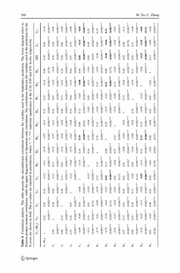
Table 4 reports the unconditional correlations between the variables used in the
bankruptcy prediction. As mentioned above, some accounting variables in Altman’s
and Ohlson’s models are highly correlated and tend to reflect similar information
about a company’s financial status. For example, the correlation between Working
capital/Total assets (V1) and Current liabilities/Current assets (W4) is quite high: the
Pearson product moment correlation coefficient is -0.79, and the Spearman rank
correlation coefficient is -0.97. Both variables measure the liquidity of the
company. For this reason, we opt for selecting predictive variables following the
stepwise approach mentioned earlier. As a result, three accounting variables, Sales/
Total assets (V4), Current liabilities/Current assets (W4), and the Dummy variable on
the net income for the last 2 years (W8) remain in the combined prediction model
for the C-score. These variables cover different aspects of business conditions,
including liquidity, profitability, solvency, and sales-generating ability.
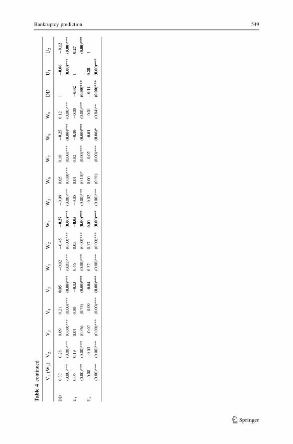
In the X-score model, which incorporates the unique Japanese institutional
features of main banks and business groups, we use the same three accounting
variables chosen from the accounting variable-based models, the computed
distance-to-default variable from the option pricing theory-based model, bank
dependence and Keiretsu dependence. The calculated correlations of these six
variables show that they are not highly correlated. The largest absolute value of the
correlation occurs between DD and W4. Both are based on the asset liability ratio,
with one using current liabilities and the market value of assets and the other using a
mixture of the book value of current liabilities and current assets. As anticipated,
DD is negatively correlated with the negative net income indicator, W8, and is
positively correlated with sales level indicator, V5. U1 and U2 are positively related,
which indicates that the Keiretsu group companies tend to be more highly controlled
by financial institutions. DD is negatively correlated with U1 and U2, and the
correlation coefficients are economically small though statistically significant. This
indicates that U1 and U2 might capture different characteristics of Japanese
companies from what DD captures. Actually, U1 and U2 are basically unrelated to
the other variables except for W1, which represents firm size. Overall, the low
correlations among these variables facilitate the interpretation of the regression
results presented in the next section.
Bankruptcy prediction 547
123
Ta
ble
4C
orr
elat
ion
anal
ysi
s.T
his
tab
lep
rese
nts
the
un
cond
itio
nal
corr
elat
ion
sb
etw
een
the
var
iab
les
use
din
the
ban
kru
ptc
yp
red
icti
on
.T
he
low
erd
iagon
alre
fers
to
Pea
rso
np
rod
uct
mom
ent
corr
elat
ion
s,w
hil
eth
eu
pp
erd
iago
nal
refe
rsto
Sp
earm
anra
nk
corr
elat
ion
s.T
he
corr
elat
ion
sb
etw
een
the
var
iab
les
use
din
the
pre
dic
tion
for
the
X-s
core
are
sho
wn
inb
old
.T
he
p-v
alu
esar
ere
po
rted
inp
aren
thes
es,
wh
ere
*,
**
,*
**
repre
sen
tsi
gn
ifica
nce
atth
e0
.10,
0.0
5an
d0
.01
lev
els,
resp
ecti
vel
y
V1
(W3)
V2
V3
V4
V5
W1
W2
W4
W5
W6
W7
W8
W9
DD
U1
U2
V1
(W3)
10.5
2
(0.0
0)*
**
0.2
5
(0.0
0)*
**
0.5
6
(0.0
0)*
**
-0.1
2
(0.0
0)*
**
-0.1
1
(0.0
0)*
**
-0.7
0
(0.0
0)*
**
-0.9
7
(0.0
0)*
**
-0.1
1
(0.0
0)*
**
0.3
3
(0.0
0)*
**
0.3
7
(0.0
0)*
**
-0.1
4
(0.0
0)*
**
0.0
0
(0.7
6)
0.3
9
(0.0
0)*
**
0.0
4
(0.0
0)*
**
-0.1
0
(0.0
0)*
**
V2
0.4
6
(0.0
0)*
**
10.3
6
(0.0
0)*
**
0.6
0
(0.0
0)*
**
-0.1
1
(0.0
0)*
**
0.1
3
(0.0
0)*
**
-0.7
2
(0.0
0)*
**
-0.5
7
(0.0
0)*
**
-0.1
1
(0.0
0)*
**
0.4
1
(0.0
0)*
**
0.6
1
(0.0
0)*
**
-0.2
5
(0.0
0)*
**
-0.0
4
(0.0
0)*
**
0.3
6
(0.0
0)*
**
0.2
8
(0.0
0)*
**
-0.0
4
(0.0
0)*
**
V3
0.0
6
(0.0
0)*
**
0.1
5
(0.0
0)*
**
10.4
6
(0.0
0)*
**
0.1
1
(0.0
0)*
**
0.0
3
(0.0
0)*
**
-0.3
2
(0.0
0)*
**
-0.2
4
(0.0
0)*
**
-0.0
9
(0.0
0)*
**
0.8
6
(0.0
0)*
**
0.7
3
(0.0
0)*
**
-0.4
1
(0.0
0)*
**
0.2
9
(0.0
0)*
**
0.3
8
(0.0
0)*
**
0.0
4
(0.0
0)*
**
-0.0
9
(0.0
0)*
**
V4
0.3
2
(0.0
0)*
**
0.1
6
(0.0
0)*
**
0.0
7
(0.0
0)*
**
1-
0.1
2
(0.0
0)*
**
-0.0
6
(0.0
0)*
**
-0.7
4
(0.0
0)*
**
-0.6
1
(0.0
0)*
**
-0.0
8
(0.0
0)*
**
0.5
2
(0.0
0)*
**
0.6
4
(0.0
0)*
**
-0.1
9
(0.0
0)*
**
0.0
4
(0.0
0)*
**
0.5
7
(0.0
0)*
**
0.1
9
(0.0
0)*
**
-0.0
8
(0.0
0)*
**
V5
-0.0
9
(0.0
0)*
**
-0.0
9
(0.0
0)*
**
0.0
3
(0.0
0)*
**
-0.0
8
(0.0
0)*
**
1-
0.1
5
(0.0
0)*
**
0.1
6
(0.0
0)*
**
0.1
9
(0.0
0)*
**
0.0
0
(0.8
4)
0.1
2
(0.0
0)*
**
-0.0
3
(0.0
0)*
**
-0.0
8
(0.0
0)*
**
0.0
4
(0.0
0)*
**
0.0
5
(0.0
0)*
**
-0.1
4
(0.0
0)*
**
-0.0
3
(0.0
0)*
**
W1
-0.1
1
(0.0
0)*
**
0.1
4
(0.0
0)*
**
0.0
1
(0.1
5)
-0.1
0
(0.0
0)*
**
-0.1
2
(0.0
0)*
**
10.1
6
(0.0
0)*
**
0.1
0
(0.0
0)*
**
-0.0
4
(0.0
0)*
**
-0.0
2
(0.0
0)*
**
0.0
3
(0.0
0)*
**
-0.1
1
(0.0
0)*
**
-0.0
1
(0.0
4)*
*
0.0
0
(0.6
5)
0.4
9
(0.0
0)*
**
0.2
9
(0.0
0)*
**
W2
-0.7
5
(0.0
0)*
**
-0.6
1
(0.0
0)*
**
-0.0
9
(0.0
0)*
**
-0.3
9
(0.0
0)*
**
0.1
5
(0.0
0)*
**
0.1
5
(0.0
0)*
**
10.7
6
(0.0
0)*
**
0.1
2
(0.0
0)*
**
-0.4
2
(0.0
0)*
**
-0.6
3
(0.0
0)*
**
0.1
5
(0.0
0)*
**
-0.0
1
(0.0
2)*
*
-0.4
8
(0.0
0)*
**
0.0
5
(0.0
0)*
**
0.1
9
(0.0
0)*
**
W4
-0.7
9
(0.0
0)*
**
-0.3
9
(0.0
0)*
**
-0.0
1
(0.1
3)
-0.2
1
(0.0
0)*
**
0.0
3
(0.0
0)*
**
0.1
1
(0.0
0)*
**
0.6
0
(0.0
0)*
**
10.1
0
(0.0
0)*
**
-0.3
3
(0.0
0)*
**
-0.4
3
(0.0
0)*
**
0.1
3
(0.0
0)*
**
0.0
0
(0.7
9)
-0.4
0
(0.0
0)*
**
-0.0
4
(0.0
0)*
**
0.1
1
(0.0
0)*
**
W5
-0.2
5
(0.0
0)*
**
-0.2
7
(0.0
0)*
**
-0.0
2
(0.0
0)*
**
-0.0
2
(0.0
0)*
**
0.0
1
(0.3
7)
-0.0
4
(0.0
0)*
**
0.2
7
(0.0
0)*
**
0.2
3
(0.0
0)*
**
1-
0.1
0
(0.0
0)*
**
-0.0
9
(0.0
0)*
**
0.1
5
(0.0
0)*
**
-0.0
3
(0.0
0)*
**
-0.0
7
(0.0
0)*
**
-0.0
5
(0.0
0)*
**
-0.0
1
(0.0
3)*
*
W6
0.0
7
(0.0
0)*
**
0.1
2
(0.0
0)*
**
0.9
1
(0.0
0)*
**
0.0
3
(0.0
0)*
**
0.0
1
(0.0
2)*
*
0.0
1
(0.1
0)*
-0.0
8
(0.0
0)*
**
-0.0
4
(0.0
0)*
**
-0.0
5
(0.0
0)*
**
10.7
2
(0.0
0)*
**
-0.4
6
(0.0
0)*
**
0.4
0
(0.0
0)*
**
0.4
5
(0.0
0)*
**
0.0
0
(0.7
9)
-0.1
1
(0.0
0)*
**
W7
0.0
9
(0.0
0)*
**
0.2
2
(0.0
0)*
**
0.4
5
(0.0
0)*
**
0.1
3
(0.0
0)*
**
-0.0
1
(0.1
4)
0.0
2
(0.0
0)*
**
-0.1
6
(0.0
0)*
**
-0.0
6
(0.0
0)*
**
-0.0
2
(0.0
0)*
**
0.7
6
(0.0
0)*
**
1-
0.3
6
(0.0
0)*
**
0.1
7
(0.0
0)*
**
0.4
2
(0.0
0)*
**
0.1
1
(0.0
0)*
**
-0.0
9
(0.0
0)*
**
W8
-0.1
6
(0.0
0)*
**
-0.2
5
(0.0
0)*
**
-0.1
3
(0.0
0)*
**
-0.0
5
(0.0
0)*
**
-0.0
7
(0.0
0)*
**
-0.1
2
(0.0
0)*
**
0.1
6
(0.0
0)*
**
0.1
3
(0.0
0)*
**
0.1
5
(0.0
0)*
**
-0.0
9
(0.0
0)*
**
-0.1
5
(0.0
0)*
**
1-
0.0
2
(0.0
1)*
**
-0.2
3
(0.0
0)*
**
-0.1
0
(0.0
0)*
**
-0.0
1
(0.1
3)
W9
0.0
1
(0.2
8)
-0.0
3
(0.0
0)*
**
0.0
8
(0.0
0)*
**
0.0
3
(0.0
0)*
**
0.0
3
(0.0
0)*
**
-0.0
1
(0.3
9)
-0.0
1
(0.0
6)*
0.0
0
(0.5
7)
-0.0
4
(0.0
0)*
**
0.0
7
(0.0
0)*
**
0.0
7
(0.0
0)*
**
-0.0
1
(0.0
0)*
**
10.1
3
(0.0
0)*
**
-0.0
9
(0.0
0)*
**
-0.0
2
(0.0
0)*
**
548 M. Xu, C. Zhang
123
Ta
ble
4co
nti
nued
V1
(W3)
V2
V3
V4
V5
W1
W2
W4
W5
W6
W7
W8
W9
DD
U1
U2
DD
0.3
7
(0.0
0)*
**
0.2
8
(0.0
0)*
**
0.0
9
(0.0
0)*
**
0.2
1
(0.0
0)*
**
0.0
5
(0.0
0)*
**
-0.0
2
(0.0
1)*
**
-0.4
5
(0.0
0)*
**
-0.2
7
(0.0
0)*
**
-0.0
9
(0.0
0)*
**
0.0
5
(0.0
0)*
**
0.1
0
(0.0
0)*
**
-0.2
5
(0.0
0)*
**
0.1
2
(0.0
0)*
**
1-
0.0
6
(0.0
0)*
**
-0.1
2
(0.0
0)*
**
U1
0.0
5
(0.0
0)*
**
0.1
9
(0.0
0)*
**
0.0
1
(0.3
6)
0.0
0
(0.7
4)
-0.1
3
(0.0
0)*
**
0.4
6
(0.0
0)*
**
0.0
5
(0.0
0)*
**
-0.0
5
(0.0
0)*
**
-0.0
5
(0.0
0)*
**
0.0
1
(0.1
0)*
0.0
2
(0.0
0)*
**
-0.1
0
(0.0
0)*
**
-0.0
8
(0.0
0)*
**
-0.0
2
(0.0
0)*
**
10.2
7
(0.0
0)*
**
U2
-0.0
8
(0.0
0)*
**
-0.0
3
(0.0
0)*
**
-0.0
2
(0.0
0)*
**
-0.0
9
(0.0
0)*
**
-0.0
4
(0.0
0)*
**
0.3
2
(0.0
0)*
**
0.1
7
(0.0
0)*
**
0.0
1
(0.0
0)*
**
-0.0
2
(0.0
0)*
**
0.0
0
(0.9
1)
-0.0
2
(0.0
0)*
**
-0.0
1
(0.0
6)*
-0.0
1
(0.0
4)*
*
-0.1
1
(0.0
0)*
**
0.2
8
(0.0
0)*
**
1
Bankruptcy prediction 549
123

5 Empirical Results
The estimated coefficients of the ~Z; O and D-scores are shown in Table 5. In Panel
A on the ~Z-score, three of the five slope coefficients are significant in terms of the
Wald chi-square statistic. All the signs of the parameter estimates are in line with
our anticipations. The measure of goodness-of-fit is indicated by the likelihood ratio
index, 0.0652. The regression results for Ohlson’s model are reported in Panel B.
Only three of the variables are statistically significant. Except for the coefficients of
W2 and W7, which are insignificant, the signs of the other coefficients are consistent
with intuition. The likelihood ratio index is slightly higher than that in Panel A,
probably due to the inclusion of more explanatory variables. The estimated
coefficients of the explanatory variables in Panels A and B are quite different from
the original models. This comes as no surprise because even in the U.S. data in the
1980s, Begley et al. (1996) find that the re-estimated coefficients of these two
models change substantially from the original ones. The regression results presented
here are qualitatively in agreement with those of Altman (1968) and Ohlson (1980).
Panel C of Table 5 presents the parameter estimates for the option pricing theory-
based model (7). The estimated slope coefficient on DD is significantly negative.
The likelihood ratio index of this model is much higher than the likelihood ratios of
the accounting variable-based models. This shows that the market data do contain
information about a company’s future prospects. However, the estimated parameters
(c0, c1) differ from the theoretical value of (0, -1), indicating that the distributional
assumption implied by the geometric Brownian motion for the market value of
assets is too restrictive, the way liabilities are measured is inappropriate, or both.
More specifically, an estimate of c1 with an absolute value of less than one means
that the distance-to-default measure is too extreme, that is, some values are too large
and some values are too small, while a negative c0 means that the distance-to-
default measure is biased upwards. Perhaps converting only half of the long-term
liabilities as 1-year debt is too optimistic. While there are plenty of ways to refine
the distance-to-default measure, we leave this for future research. The flexibility
offered by the free parameters (c0, c1) serves our purpose.
Panel D of Table 5 reports the results of the C-score regression. The coefficients
of all the variables are significant at the 0.05 level by construction because the
insignificant accounting variables are left out of the model. In comparison with the
original models, the coefficients of V5, W4, W8 and DD do not change much and
their p-values are almost the same as before. The significance level does not show a
great improvement. However, there is one point worthy of attention. While the three
accounting variables are taken from financial statements only, they remain
significant when DD is added. This means that market data and financial statements
have separate information about a company’s future prospects. These variables are
complementary in predicting bankruptcy. The likelihood ratio index increases to
0.1483, much greater than either of the accounting variable-based models or the
option pricing theory-based model alone.
In Panel E of Table 5, the estimates of the model with the two Japanese
institutional variables are reported. The coefficients of U1 and U2 are significantly
negative, indicating that bank dependence and Keiretsu dependence are significantly
550 M. Xu, C. Zhang
123

Table 5 Model estimation for the full sample period (1992–2005) . This table presents the estimates of
five hazard models
~Zit ¼ Uða0 þ a1V1it þ a2V2it þ a3V3it þ a4V4it þ a5V5itÞ;Oit ¼ Uðb0 þ b1W1it þ b2W2it þ b3W3it þ b4W4it þ b5W5it þ b6W6it þ b7W7it þ b8W8it þ b9W9itÞ;Dit ¼ Uðc0 þ c1DDitÞ;Cit ¼ Uðd0 þ d1V5it þ d2W4it þ d3W8it þ d4DDitÞ;Xit ¼ Uðe0 þ e1V5it þ e2W4it þ e3W8it þ e4DDit þ e5U1it þ e6U2itÞ;where ~Z;O, D, C, and X are the bankruptcy probabilities and U is the cumulative standard normal
distribution. ** and *** represent significance at the 0.05 and 0.01 levels, respectively. The p-values that
are less than 0.0001 are marked as 0.0001. LRI is the likelihood ratio index. The number of observations
included in the regression analysis is reported as #OBS
Variable Estimate p-Value LRI #OBS
A. Altman’s model: ~Z-score
Intercept -4.1776 0.0001*** 0.0652 28,712
V1 -0.5294 0.0206**
V2 -0.2139 0.1035
V3 -1.0411 0.1219
V4 -0.4303 0.0032***
V5 -1.3183 0.0001***
B. Ohlson’s model: O-score
Intercept -5.9422 0.0001*** 0.0748 27,123
W1 -0.0813 0.3151
W2 -0.0944 0.8743
W3 -0.2189 0.7593
W4 0.2751 0.0004***
W5 -0.8617 0.4162
W6 -0.0745 0.2526
W7 0.0374 0.4479
W8 1.5211 0.0001***
W9 -0.6270 0.0039***
C. Option pricing theory based D-score
Intercept -4.5118 0.0001*** 0.1251 27,702
DD -0.5405 0.0001***
D. The combined model: C-score
Intercept -4.3803 0.0001*** 0.1483 26,086
V5 -0.6674 0.0117**
W4 0.1683 0.0009***
W8 0.7019 0.0079***
DD -0.4470 0.0001***
E. The most comprehensive model: X-score
Intercept -3.7458 0.0001*** 0.1645 26,086
V5 -0.7030 0.0086***
W4 0.1407 0.0056***
W8 0.5591 0.0367**
Bankruptcy prediction 551
123
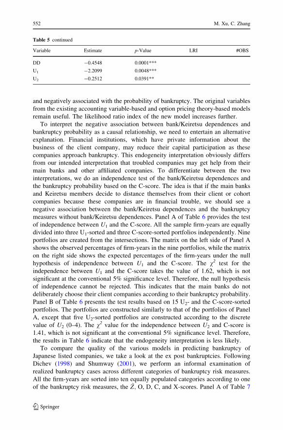
and negatively associated with the probability of bankruptcy. The original variables
from the existing accounting variable-based and option pricing theory-based models
remain useful. The likelihood ratio index of the new model increases further.
To interpret the negative association between bank/Keiretsu dependences and
bankruptcy probability as a causal relationship, we need to entertain an alternative
explanation. Financial institutions, which have private information about the
business of the client company, may reduce their capital participation as these
companies approach bankruptcy. This endogeneity interpretation obviously differs
from our intended interpretation that troubled companies may get help from their
main banks and other affiliated companies. To differentiate between the two
interpretations, we do an independence test of the bank/Keiretsu dependences and
the bankruptcy probability based on the C-score. The idea is that if the main banks
and Keiretsu members decide to distance themselves from their client or cohort
companies because these companies are in financial trouble, we should see a
negative association between the bank/Keiretsu dependences and the bankruptcy
measures without bank/Keiretsu dependences. Panel A of Table 6 provides the test
of independence between U1 and the C-score. All the sample firm-years are equally
divided into three U1-sorted and three C-score-sorted portfolios independently. Nine
portfolios are created from the intersections. The matrix on the left side of Panel A
shows the observed percentages of firm-years in the nine portfolios, while the matrix
on the right side shows the expected percentages of the firm-years under the null
hypothesis of independence between U1 and the C-score. The v2 test for the
independence between U1 and the C-score takes the value of 1.62, which is not
significant at the conventional 5% significance level. Therefore, the null hypothesis
of independence cannot be rejected. This indicates that the main banks do not
deliberately choose their client companies according to their bankruptcy probability.
Panel B of Table 6 presents the test results based on 15 U2- and the C-score-sorted
portfolios. The portfolios are constructed similarly to that of the portfolios of Panel
A, except that five U2-sorted portfolios are constructed according to the discrete
value of U2 (0–4). The v2 value for the independence between U2 and C-score is
1.41, which is not significant at the conventional 5% significance level. Therefore,
the results in Table 6 indicate that the endogeneity interpretation is less likely.
To compare the quality of the various models in predicting bankruptcy of
Japanese listed companies, we take a look at the ex post bankruptcies. Following
Dichev (1998) and Shumway (2001), we perform an informal examination of
realized bankruptcy cases across different categories of bankruptcy risk measures.
All the firm-years are sorted into ten equally populated categories according to one
of the bankruptcy risk measures, the ~Z; O, D, C, and X-scores. Panel A of Table 7
Table 5 continued
Variable Estimate p-Value LRI #OBS
DD -0.4548 0.0001***
U1 -2.2099 0.0048***
U2 -0.2512 0.0391**
552 M. Xu, C. Zhang
123

reports the estimated average bankruptcy probability for each category according to
the ~Z; O, D, C, and X-scores. As bankruptcy is a rare event, the estimated
probabilities, as measured by the ~Z; O, D, C, and X-scores, are all small. Panel B of
Table 7 reports the number of observed performance-related delistings during the
next year by the bankruptcy risk category. As we can see, all the measures are
successful in predicting bankruptcy. The majority of delistings appear in the high-
risk categories, that is, those with large ~Z; O, D, C, and X-scores. A more successful
measure captures more delisted companies in its highest-risk category.
The option pricing theory-based D-score appears to be more successful than the~Z-score and the O-score in terms of the likelihood ratio index. From Panel B of
Table 7, we see that the D-score predicts more delisted companies in the highest-
risk category than those predicted by the ~Z-score and the O-score. However,
because accounting information and market information are complementary, the C-
score successfully assigns more delisted companies into the highest-risk category
than the D-score does. By incorporating U1 and U2 into the prediction model, the X-
score further improves the prediction. As shown in Panel B of Table 7, only one
company (1.3% of all the delistings) is allocated into three lowest-risk categories by
the X-score, while 55 delisted companies (72.4% of all the delistings) are classified
Table 6 Test of independence between C-score and Japanese institutional variables. Panel A provides
the results of nine U1- and C-score-sorted portfolios. All the sample firm-years are equally classified into
three U1-sorted and three C-score-sorted portfolios independently. Nine portfolios are created from the
intersections. The matrix on the left side shows the observed percentages of firm-years in different
portfolios, while the matrix on the right side shows the percentages under the null hypothesis of inde-
pendence between U1 and the C-score. v2 is the Pearson chi-square statistics for the test of independence
between U1 and the C-score. Panel B provides the results based on 15 U2- and C-score-sorted portfolios.
The portfolios are constructed similarly to that of the portfolios of Panel A, except that five U2-sorted
portfolios are constructed according to the discrete value of U2 (0-4)
Observed percentages Percentages under the null
C-score C-score
1 (Low) 2 3 (High) Sum 1 (Low) 2 3 (High) Sum
A.
U1 1 (Low) 13.29 10.50 9.55 33.34 U1 1 (Low) 11.11 11.11 11.11 33.34
2 10.97 9.96 12.41 33.33 2 11.11 11.11 11.11 33.33
3 (High) 9.07 12.88 11.39 33.34 3 (High) 11.11 11.11 11.11 33.34
Sum 33.33 33.33 33.34 100.00 Sum 33.33 33.33 33.34 100.00
v2 of independence test = 1.62; degrees of freedom = 4; p-value = 0.81
B.
U2 0 24.39 22.90 20.84 68.13 U2 0 22.71 22.71 22.71 68.13
1 3.52 3.45 3.98 10.94 1 3.65 3.65 3.65 10.94
2 1.92 2.23 2.43 6.59 2 2.20 2.20 2.20 6.59
3 2.43 2.27 3.43 8.14 3 2.71 2.71 2.71 8.14
4 1.07 2.48 2.65 6.19 4 2.06 2.06 2.07 6.19
Sum 33.33 33.33 33.34 100.00 Sum 33.33 33.33 33.34 100.00
v2 of independence test = 1.41; degrees of freedom = 8; p-value = 0.99
Bankruptcy prediction 553
123

into the two highest-risk categories. In sum, each of the five models appears to be
fairly accurate, assigning between 59.2% and 72.4% of delistings to the two highest-
risk categories. By incorporating the unique features of the Japanese institutions, the
X-score is economically better.
An important aspect of the relationship between the bank/Keiretsu dependences
and the bankruptcy probability is its cross-sectional implication: at any given point
of time, companies with closer ties to their main banks and group members have
less chance to go bankrupt. From Table 2, however, we see a strong time-series
correlation between the number of bankruptcies per year and the average bank/
Keiretsu dependences from that year. Basically, the number of bankruptcies
increased over time while the average bank/Keiretsu dependences decreased. The
decreasing pattern is particularly strong for average bank dependence. Is the result
of the negative relationship between bankruptcy probability and bank/Keiretsu
dependences reported in Panel E of Table 5 using panel data mainly driven by the
time-series property? If it is and the cross-sectional effect is absent, the result might
be spurious. In other words, the increase in the number of bankruptcies over time
Table 7 Comparison of the bankruptcy measures in predicting performance-related delistings. All the
sample firm-years are equally sorted into ten categories according to their bankruptcy scores. Panel A
reports the estimated average bankruptcy probability for each category. Panel B reports the number of
actual performance-related delisting cases in each bankruptcy-risk-sorted category
Category ~Z-score O-score D-score C-score X-score
A. Average bankruptcy scores
1 (Low risk) 0.0001 0.0010 0.0007 0.0004 0.0002
2 0.0006 0.0013 0.0007 0.0006 0.0004
3 0.0010 0.0014 0.0007 0.0007 0.0006
4 0.0015 0.0016 0.0007 0.0008 0.0008
5 0.0019 0.0017 0.0007 0.0009 0.0010
6 0.0024 0.0019 0.0007 0.0011 0.0012
7 0.0029 0.0021 0.0016 0.0016 0.0016
8 0.0035 0.0026 0.0025 0.0025 0.0022
9 0.0046 0.0036 0.0046 0.0043 0.0041
10 (High risk) 0.0081 0.0109 0.0146 0.0161 0.0169
B. In-sample prediction test
1 (Low risk) 2 6 3 2 1
2 4 4 3 3 0
3 1 2 3 3 0
4 5 1 2 2 4
5 3 4 3 2 3
6 4 1 3 0 5
7 4 8 4 5 2
8 5 5 7 9 6
9 16 10 7 6 9
10 (High risk) 32 35 41 44 46
554 M. Xu, C. Zhang
123

might just have happened when the average bank/Keiretsu dependences decreased
over time, while there is no relationship between bank/Keiretsu dependences and
bankruptcy probability at any given point of time.
An ideal way to determine whether the reported negative relationships exist only
in time-series or in both time-series and cross-sections, if the data allow, is to run
cross-sectional regressions every year. Unfortunately, because the number of
bankruptcies per year is small, especially in the early years of the sample, the cross-
sectional regressions lack the power to detect most of the relationships, not just the
bank/Keiretsu dependences. An alternative approach, which is as effective as the
cross-sectional regressions, is to run the following hazard regression model:
Xit ¼ Uðe1T1t þ e2T2t þ e3T3t þ e4V5it þ e5W4it þ e6W8it þ e7DDit þ e8U1it
þ e9U2itÞ; ð10Þ
where T1 is the dummy variable for 1992–1997, T2 is the dummy for 1998–2001,
and T3 is the dummy for 2002–2005. The division into the three subperiods follows
the observed pattern of U1 in Table 2. We expect the coefficients of these dummies
to increase over the subperiods, capturing the increasing pattern of the number of
bankruptcy cases over time. If the negative relationships between the bankruptcy
probability and the bank/Keiretsu dependences are a time-series property only, we
expect to see insignificant coefficients of U1 and U2. The result of the estimated
regression model is reported in Table 8.
The results in Table 8 show that there is indeed a time-series effect: the
coefficients of the subperiod dummies increase over the subperiods. Compared with
Panel E of Table 5, the coefficients of U1 and U2 are slightly smaller, but they
Table 8 Test of a potentially spurious relationship. This table presents the estimates of the following
hazard model:
Xit ¼ Uðe1T1t þ e2T2t þ e3T3t þ e4V5it þ e5W4it þ e6W8it þ e7DDit þ e8U1it þ e9U2itÞ;
where X is the bankruptcy probability and U is the cumulative standard normal distribution. T1 is the
dummy variable for 1992–1997, T2 is the dummy variable for 1998–2001, and T3 is the dummy variable
for 2002–2005. ** and *** represent significance at the 0.05 and 0.01 levels, respectively. The p-values
that are less than 0.0001 are marked as 0.0001. LRI is the likelihood ratio index. The number of
observations included in the regression analysis is reported as #OBS
Variable Estimate p-Value LRI #OBS
T1 -3.8156 0.0001*** 0.1656 26,086
T2 -3.7409 0.0001***
T3 -3.5004 0.0001***
V5 -0.6943 0.0095***
W4 0.1420 0.0054***
W8 0.5555 0.0383**
DD -0.4455 0.0001***
U1 -2.6596 0.0082***
U2 -0.2495 0.0412**
Bankruptcy prediction 555
123
remain highly significant. The result shows that the relationship between the bank/
Keiretsu dependences and bankruptcy probability is a cross-sectional property as
well as a time-series one.
As is always the case when comparing bankruptcy prediction models, out-of-
sample prediction should be the ultimate criterion, while in-sample performance
may result from over-fitting of the data. To see how the models perform out of
sample, we estimate all the bankruptcy scores with data from 1992–2003 and use
the estimated coefficients to predict bankruptcy in the hold-out sample period of
2004–2005. The results of the model estimation for the period 1992–2003 are
virtually the same as those reported in Table 5. The predictive power of the five
models is robust. Most of the bankruptcy cases in 2004–2005 are classified in the
two highest-risk deciles, while very few cases appear in the three lowest-risk
deciles. As expected, the C-score model and the X-score model fare the best, and the
other models are about equally good. These results are not reported to save the
space.
6 Concluding remarks
In this paper, we investigate bankruptcy prediction of Japanese listed companies.
Accounting variables used in Altman’s Z-score, Ohlson’s O-score and the option
pricing theory-based distance-to-default measure, previously developed for the U.S.
market, are useful in predicting bankruptcy of Japanese companies. Traditional
accounting variables form the basis for predicting bankruptcy, while the stock
market variables provide more forward-looking information about a company’s
future prospects. We find that, for Japanese listed companies, the option pricing
theory-based bankruptcy measure is more successful than the accounting variable-
based measures alone, but it does not subsume the accounting measures. These
variables and models all have their own strengths and cover certain aspects of
bankruptcy prediction. When the two sets of variables are combined together, the
predictive power of the model improves substantially. Instead of picking a winner
among them, a more meaningful question in future research is how we should better
combine the models to produce better predictions.
The Japanese economy is unique because of its main bank system and Keiretsu
structure. A new X-score is proposed to capture these special features. It
incorporates a variable representing a company’s bank dependence, a variable
representing a company’s Keiretsu dependence and some important ingredients
from the existing bankruptcy prediction models. The negative relationships between
bankruptcy probability and the bank/Keiretsu dependences are genuine cross-
sectional relationships, which also exhibit a time-series pattern. The X-score further
improves bankruptcy prediction of Japanese listed companies.
Acknowledgements We are grateful to James Ohlson (editor) and two anonymous reviewers for their
insightful suggestions that have substantially improved the paper. We also thank Lewis Chan, Kevin
Chen, Steven Wei, Xueping Wu, and seminar participants at the Hong Kong University of Science and
Technology, University of Macau, the Shanghai University of Finance and Economics, the 2004 FMA
European Conference, the 2005 AsianFA Annual Conference, and the 18th Australasian Finance and
556 M. Xu, C. Zhang
123

Banking Conference for helpful comments and suggestions. All errors are our own. Ming Xu gratefully
acknowledges the financial support provided by the Hong Kong Polytechnic University Departmental
Research Grant.
References
Altman, E. (1968). Financial ratios, discriminant analysis and the prediction of corporate bankruptcy.
Journal of Finance,23, 589–609.
Altman, E. (1993). Corporate financial distress and bankruptcy: A complete guide to predicting andavoiding distress and profiting from bankruptcy. NY: Wiley.
Altman, E., Haldeman, R. G., & Narayanan, P. (1977). Zeta analysis: a new model to identify bankruptcy
risk of corporations. Journal of Banking and Finance,10, 29–54.
Beaver, W. (1966). Financial ratios as predictors of bankruptcy. Journal of Accounting Research,6, 71–
102.
Beaver, W. (1968). Market prices, financial ratios, and the prediction of failure. Journal of AccountingResearch,8, 179–192.
Beaver, W., McNichols, M., & Rhie, J. (2005). Have financial statements become less informative?
Evidence from the ability of financial ratios to predict bankruptcy. Review of Accounting Studies,10,
93–122.
Begley, J., Ming, J., & Watts, S. (1996). Bankruptcy classification errors in the 1980s: An empirical
analysis of Altman’s and Ohlson’s models. Review of Accounting Studies,1, 267–284.
Bharath, S., & Shumway, T. (2005). Forecasting default with the KMV-Merton model, Working
paper, University of Michigan. http://w4.stern.nyu.edu/salomon/docs/Credit2006/shumway_kmv
merton1.pdf.
Black, F., & Scholes, M. (1973). The pricing of options and corporate liabilities. Journal of PoliticalEconomy,81, 637–659.
Bris, A., Welch, I., & Zhu, N. (2006). The costs of bankruptcy: Chapter 7 Liquidation versus Chapter 11
Reorganization. Journal of Finance,61, 1253–1303.
Brockman, P., & Turtle, H. (2003). A barrier option framework for corporate security valuation. Journalof Financial Economics,67, 511–530.
Brown & Company Ltd. Industrial Groupings in Japan. Various issues.
Campbell, J., Hilscher, J., & Szilagyi, J. (2007). In search of distress risk, Working paper, Harvard
University. http://www.econ.nyu.edu/user/galed/fewpapers/FEW%20S07/Campbell-Hilscher-Szila
gyi.pdf.
Charitou, A., & Trigeorgis, L., (2004). Explaining bankruptcy using option theory, Working paper, University
of Cyprus. http://www.pba.ucy.ac.cy/courses/2004_11_TAR_Option_Bankr_2411_04.pdf.
Chava, S., & Jarrow, R. (2004). Bankruptcy prediction with industry effects. Review of Finance,8, 537–
569.
Crosbie, P., & Bohn, J. (2002). Modeling default risk. KMV.
Dichev, I. (1998). Is the risk of bankruptcy a systematic risk? Journal of Finance,53, 1131–1147.
Duffie, D., Saita, L., & Wang, K. (2007). Multi-period corporate default prediction with stochastic
covariates. Journal of Financial Economics,83, 635–665.
Flath, D. (2001). Japan’s business groups, Chapter 11. In M. Nakamura (Ed.), The Japanese business andeconomic system: History and prospects for the 21st century. Palgrave Macmillan.
Hillegeist, S., Keating, E., Cram, D., & Lundstedt, K. (2004). Assessing the probability of bankruptcy.
Review of Accounting Studies,9, 5–34.
Hoshi, T., & Kashyap, A. (2001). Corporate financing and governance in Japan: The road to the future.
The MIT Press.
Hoshi, T., Kashyap, A., & Scharfstein, D. (1990). The role of banks in reducing the costs of financial
distress in Japan. Journal of Financial Economics,27, 67–88.
Leland, H. (2004). Predictions of expected default probabilities in structural models of debt. Journal ofInvestment Management,2, 1–28.
Merton, R. C. (1973). Theory of rational option pricing. Bell Journal of Economics and ManagementScience,4, 141–183.
Merton, R. C. (1974). On the pricing of corporate debt: The risk structure of interest rates. Journal ofFinance,29, 449–470.
Bankruptcy prediction 557
123

Miwa, Y., & Mark Ramseyer, J. (2005). Conflicts of Interest in Japanese Insolvencies: The Problem of
Bank Rescues. Theoretical Inquiries in Law,6, 301.
Nakamura, M. (2006). Japanese corporate governance practices in the post-bubble era: Implications of
institutional and legal reforms in the 1990s and early 2000s. International Journal of Disclosure andGovernance,3, 233–261.
Ohlson, J. (1980). Financial ratios and the probabilistic prediction of bankruptcy. Journal of AccountingResearch,18, 109–131.
Shread, P. (1989). The main bank system and corporate monitoring and control in Japan. Journal ofEconomic Behavior,11, 399–422.
Shread, P. (1994). Main banks and the governance of financial distress. In M. Aoki & H. Patrick (Eds.),
The Japanese main bank system: Its relevancy for developing and transforming economies. Oxford
University Press.
Shumway, T. (2001). Forecasting bankruptcy more accurately: a simple hazard model. Journal ofBusiness,74, 101–124.
Suzuki, S., & Wright, R. W. (1985). Financial structure and bankruptcy risk in Japanese companies.
Journal of International and Business Studies,16, 97–110.
Vassalou, M., & Xing, Y. (2004). Default risk in equity returns. Journal of Finance,59, 831–868.
Xu, P. (2004). Bankruptcy Resolution in Japan: corporation Reorganization vs. Civil Rehabilitation,
Working paper, Hosei University. http://www.rieti.go.jp/en/events/03010801/pdf/Xu_p.pdf.
Zmijewski, M. E. (1984). Methodological issues related to the estimation of financial distress prediction
models. Journal of Accounting Research,22, 59–82.
558 M. Xu, C. Zhang
123


