

BEAR Essentials
Overview of the Berkeley Energy and Resources Model
David Roland-Holst Department of Agricultural and Resource Economics [email protected]
10 April 2015

Roland-Holst 2 10 April 2015
Objectives
1. Estimate direct and economywide indirect impacts and identify adjustment patterns (BEAR).
2. Inform stakeholders and improve visibility for policy makers.
3. Promote empirical standards for policy research and dialogue.
Roland-Holst 3 10 April 2015
Why a state model?
1. California needs research capacity to support its own policies
• A first-tier world economy
2. California is unique • Both economic structure and emissions
patterns differ from national averages
3. California stakeholders need more accurate information about the adjustment process
• National assessment masks interstate spillovers and trade-offs

Roland-Holst 4 10 April 2015
Why a General Equilibrium Model?
1. Complexity - Given the complexity of today’s economy, policy makers relying on intuition and rules-of-thumb alone are assuming substantial risks.
2. Linkage - Indirect effects of policies often outweigh direct effects.
3. Political sustainability - Economic policy may be made from the top down, but political consequences are often felt from the bottom up. These models identify stakes and stakeholders before policies are implemented.
Roland-Holst 5 10 April 2015
Primary Components
The Berkeley Energy And Resource (BEAR) modeling facility stands on two legs:
1. Detailed economic and emissions data
2. A dynamic GE forecasting model
Roland-Holst 6 10 April 2015
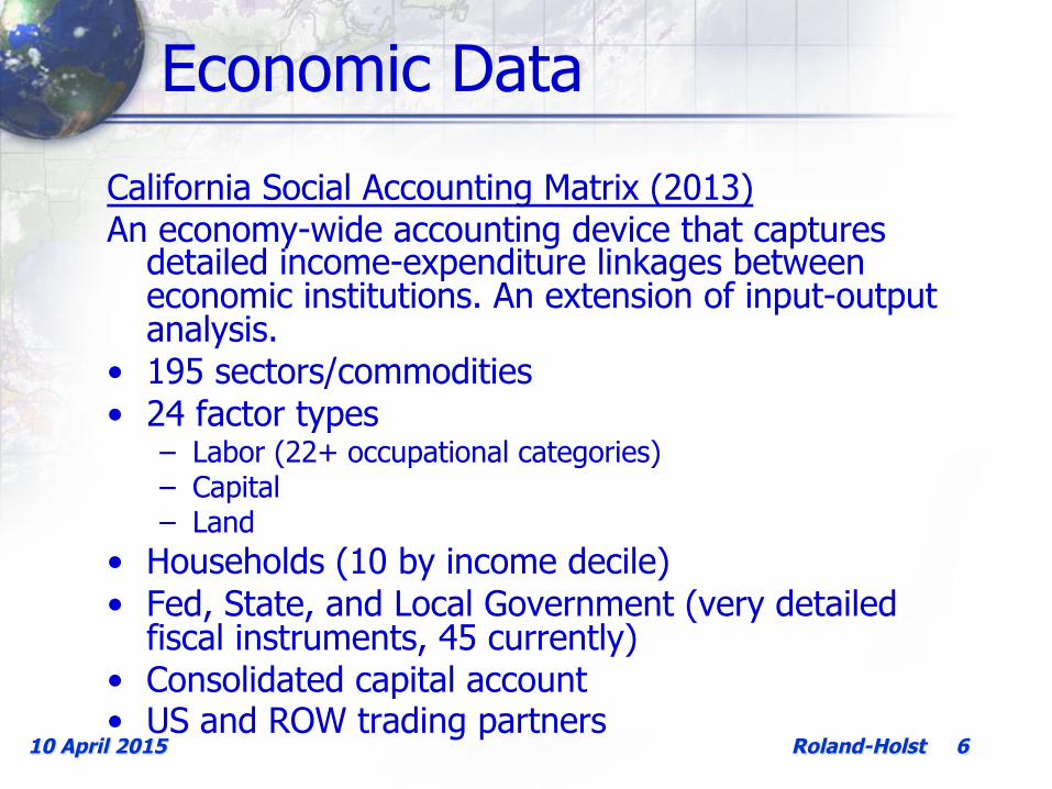
Economic Data
California Social Accounting Matrix (2013) An economy-wide accounting device that captures
detailed income-expenditure linkages between economic institutions. An extension of input-output analysis.
• 195 sectors/commodities • 24 factor types
– Labor (22+ occupational categories) – Capital – Land
• Households (10 by income decile) • Fed, State, and Local Government (very detailed
fiscal instruments, 45 currently) • Consolidated capital account • US and ROW trading partners
Roland-Holst 7 10 April 2015
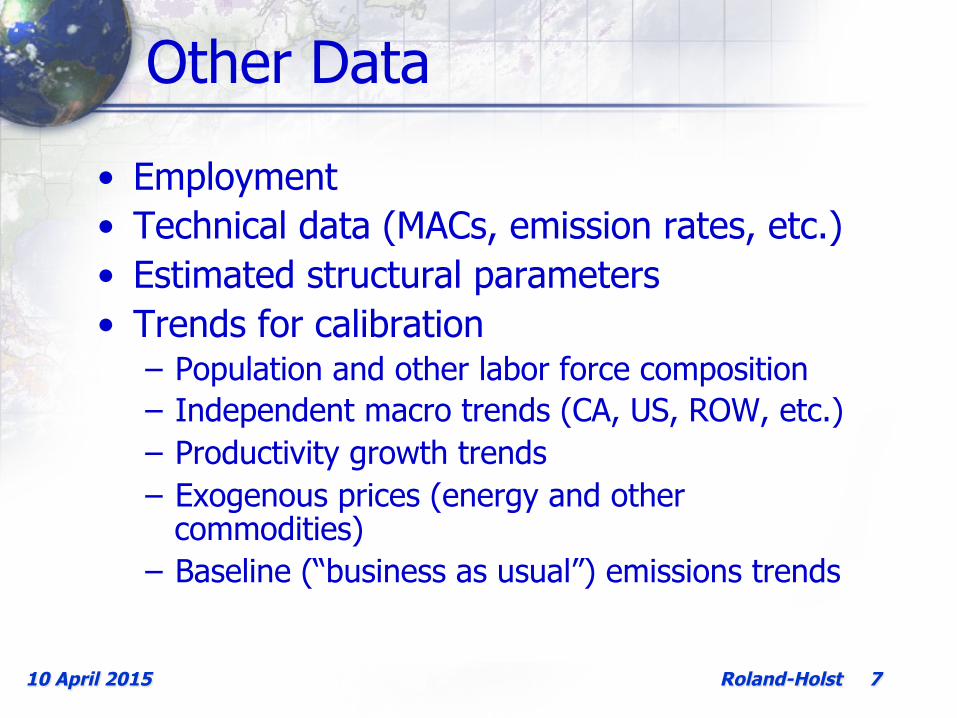
Other Data
• Employment • Technical data (MACs, emission rates, etc.) • Estimated structural parameters • Trends for calibration
– Population and other labor force composition – Independent macro trends (CA, US, ROW, etc.) – Productivity growth trends – Exogenous prices (energy and other
commodities) – Baseline (“business as usual”) emissions trends
Roland-Holst 8 10 April 2015
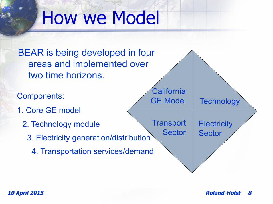
How we Model
California GE Model
Transport Sector
Electricity Sector
Technology
BEAR is being developed in four areas and implemented over two time horizons.
Components:
1. Core GE model
2. Technology module
3. Electricity generation/distribution
4. Transportation services/demand
Roland-Holst 9 10 April 2015
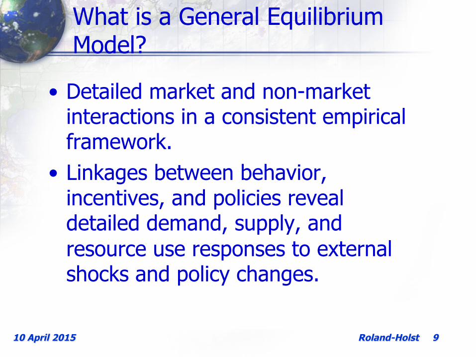
What is a General Equilibrium Model?
• Detailed market and non-market interactions in a consistent empirical framework.
• Linkages between behavior, incentives, and policies reveal detailed demand, supply, and resource use responses to external shocks and policy changes.

Roland-Holst 10 10 April 2015
Technology
• Technology is a primary determinant of resource use patterns
• Currently, all technical efficiency is exogenously specified (share, elasticity, and productivity parameters)
• Future versions of the model will incorporate endogenous technological change

Roland-Holst 11 10 April 2015
Electricity Sector Modeling
Power generation accounts for a significant percentage of C02 emissions within California.
To understand how this sector will adjust to policy changes, it is essential to capture its economic and technical heterogeneity
Based on detailed producer data from CEC/PIER/PROSYM, we model technology and emissions in California’s electricity sector – Eight generation technologies – Eleven fuels
Roland-Holst 12 10 April 2015
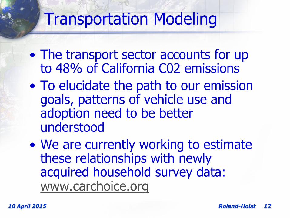
Transportation Modeling
• The transport sector accounts for up to 48% of California C02 emissions
• To elucidate the path to our emission goals, patterns of vehicle use and adoption need to be better understood
• We are currently working to estimate these relationships with newly acquired household survey data: www.carchoice.org
Roland-Holst 13 10 April 2015
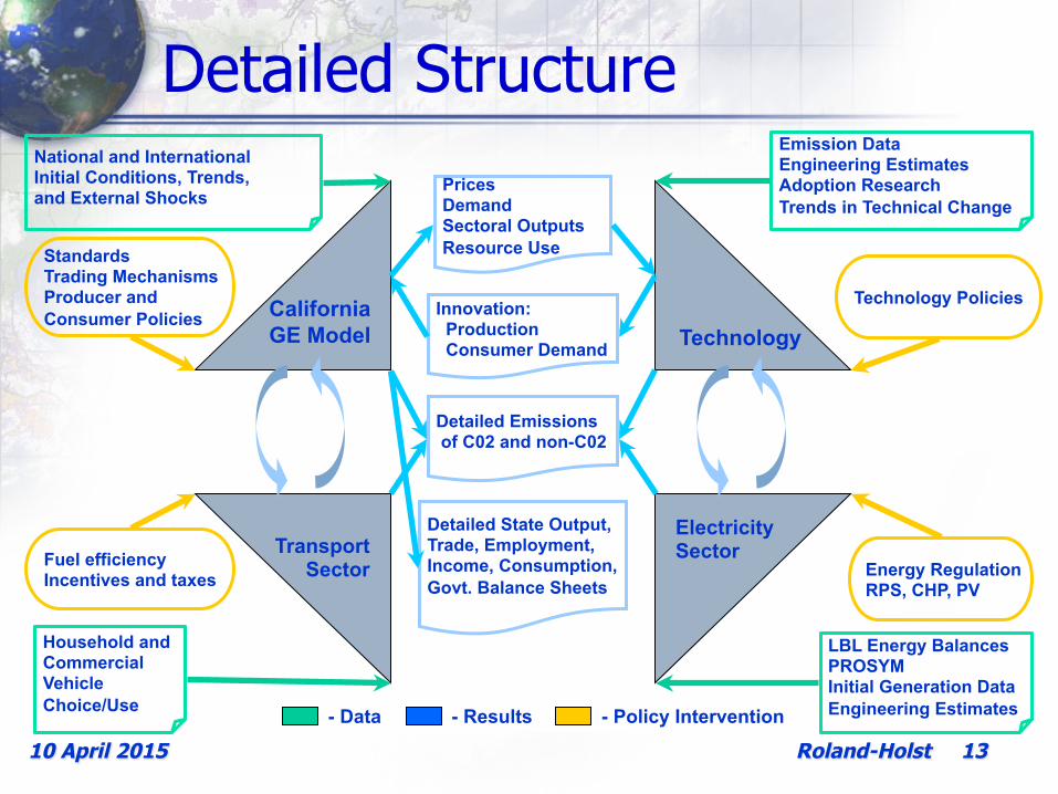
Detailed Structure National and International Initial Conditions, Trends, and External Shocks
Emission Data Engineering Estimates Adoption Research Trends in Technical Change
Prices Demand Sectoral Outputs Resource Use
Detailed State Output, Trade, Employment, Income, Consumption, Govt. Balance Sheets
Standards Trading Mechanisms Producer and Consumer Policies
Technology Policies
California GE Model
Transport Sector
Electricity Sector
Technology
LBL Energy Balances PROSYM Initial Generation Data Engineering Estimates
Innovation: Production Consumer Demand
Energy Regulation RPS, CHP, PV
- Data - Results - Policy Intervention
Household and Commercial Vehicle Choice/Use
Fuel efficiency Incentives and taxes
Detailed Emissions of C02 and non-C02
Roland-Holst 14
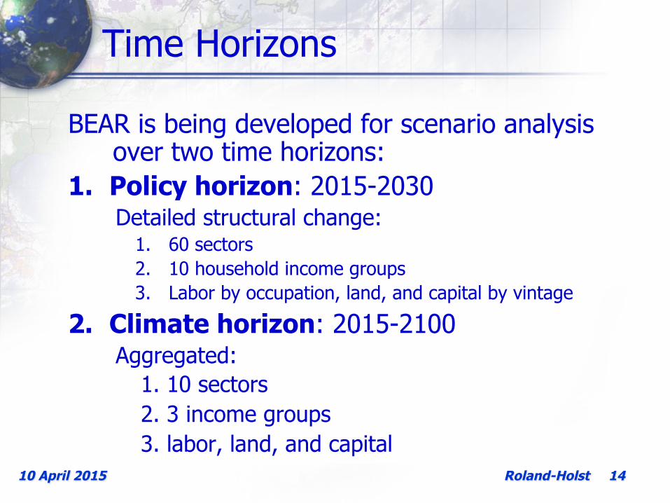
Time Horizons
BEAR is being developed for scenario analysis over two time horizons:
1. Policy horizon: 2015-2030 Detailed structural change:
1. 60 sectors 2. 10 household income groups 3. Labor by occupation, land, and capital by vintage
2. Climate horizon: 2015-2100 Aggregated:
1. 10 sectors 2. 3 income groups 3. labor, land, and capital
10 April 2015

Roland-Holst 15 10 April 2015
BEAR Model Structure
Roland-Holst 16 10 April 2015
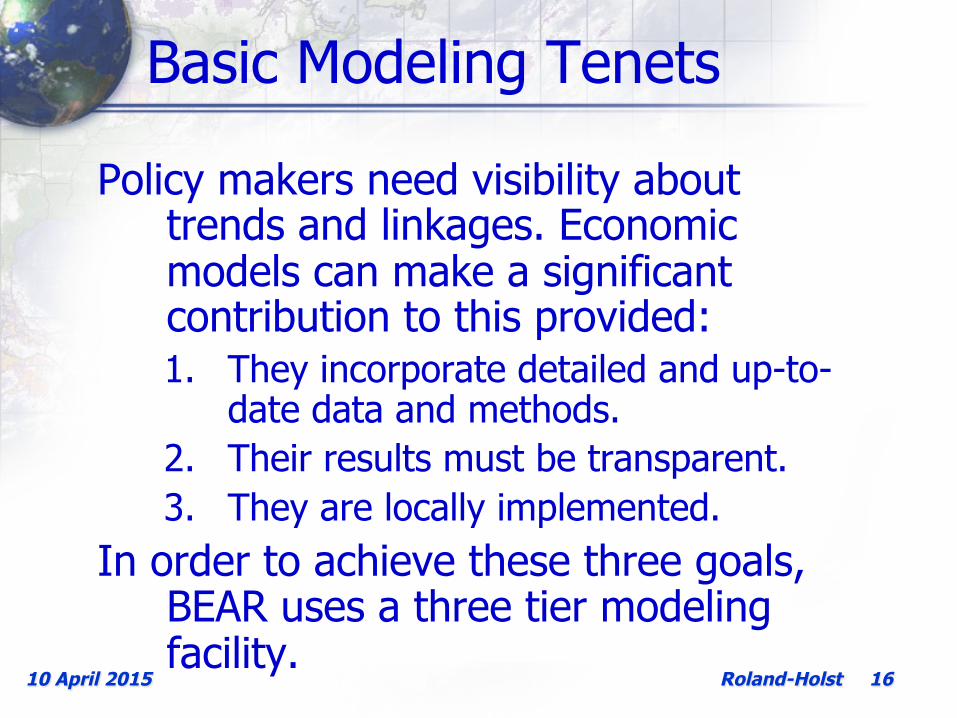
Basic Modeling Tenets
Policy makers need visibility about trends and linkages. Economic models can make a significant contribution to this provided: 1. They incorporate detailed and up-to-
date data and methods. 2. Their results must be transparent. 3. They are locally implemented.
In order to achieve these three goals, BEAR uses a three tier modeling facility.

Roland-Holst 17 10 April 2015
Schematic Modeling Facility
Social Accounting
Matrix
Econometric Parameter Estimates
Policy
Scenarios
CGE Model Baseline
Calibration Data
Numerical Results GIS Mapping
Initial Conditions
Simulation
Dissemination
Software Implementation: Excel GAMS ArcGIS
Roland-Holst 18 10 April 2015
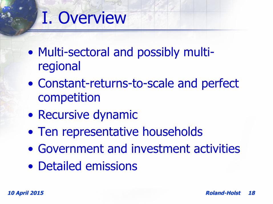
I. Overview
• Multi-sectoral and possibly multi-regional
• Constant-returns-to-scale and perfect competition
• Recursive dynamic • Ten representative households • Government and investment activities • Detailed emissions

Roland-Holst 19 10 April 2015
II. Production
• Supply – Firm-level production technology with Leontief intermediate use.
• Two production archetypes: – Agriculture (extensive vs. intensive),
including land, energy and agricultural chemicals as substitutable inputs
– Other (standard capital-labor substitution) • Labor, Capital, Land, and Energy (by
fuel type) are factors of production

Roland-Holst 20 10 April 2015
Nested Production Structure
Output
Intermediate Demand by Region
Capital Demand Energy Bundle
Labor Demand by Skill Type
Capital-Energy (KE)
Labor Bundle
Capital-Energy-Labor Bundle (KEL) Non-energy Intermediate Bundle
Energy Demand by Fuel Type Capital by Vintage
CES
CES
CES
CES
CES CES CES

Roland-Holst 21 10 April 2015
III. Capital and Land
• Two vintages of capital, old (sector specific) and new (mobile), each with its own productivity and relative price
• Land is specific to agriculture, but “mobile” between agricultural products

Roland-Holst 22 10 April 2015
IV. Labor
• Supplied by households in response to a labor-leisure choice
• Employed by sector and occupation, with perfect mobility between the former and none (currently) between the latter
• Labor markets are perfectly competitive
• Migration is not currently modeled

Roland-Holst 23 10 April 2015
V. Households
• Ten representative household categories, but state income tax bracket
• Income from all factors, enterprises, public and private transfers
• Consumption modeled with the Extended Linear Expenditure System
• Extensive tax and transfer mechanisms • Demographic dynamics (population, labor
force participation)
Roland-Holst 24 10 April 2015
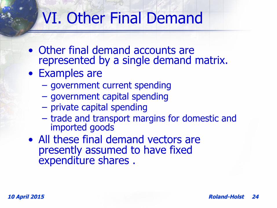
VI. Other Final Demand
• Other final demand accounts are represented by a single demand matrix.
• Examples are – government current spending – government capital spending – private capital spending – trade and transport margins for domestic and
imported goods • All these final demand vectors are
presently assumed to have fixed expenditure shares .

Roland-Holst 25 10 April 2015
VII. Government
• Government is a passive actor in the baseline, adhering to established expenditure patterns and fiscal programs
• The model details extensive accounting for transfer relationships between institutions (fiscal, capital flows, remittances, etc.).
• Government behavior is a primary driver of scenarios, but this behavior remains largely exogenous (subject to fiscal closure)

Roland-Holst 26 10 April 2015
• Demand is thought to combine in-state and imported goods in each product category with a nested CES aggregation
• Output is modeled symmetrically with a dual nested CET structure
VIII. Trade
Imports/Exports In-State Goods
Aggregate Demand/Supply
Rest of USA Rest of World
CES/CET
CES/CET
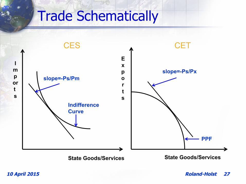
Roland-Holst 27 10 April 2015
Trade Schematically
State Goods/Services
Impor t s
Indifference Curve
slope=-Ps/Pm
State Goods/Services
Exports
PPF
slope=-Ps/Px
CES CET
Roland-Holst 28 10 April 2015
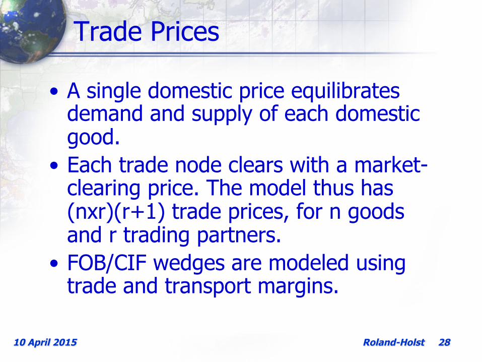
Trade Prices
• A single domestic price equilibrates demand and supply of each domestic good.
• Each trade node clears with a market-clearing price. The model thus has (nxr)(r+1) trade prices, for n goods and r trading partners.
• FOB/CIF wedges are modeled using trade and transport margins.
Roland-Holst 29 10 April 2015
IX. Equilibrium Conditions
• Combined in-state and external demand equal supply for every good and service
• In-state factor (labor, land, capital) supply equals in-state factor demand
• California’s net outflow of goods and services equals its net claims on external financial assets

Roland-Holst 30 10 April 2015
X. Macroeconomic Closure
• Taxes on intermediate inputs and final demand, factors of production, output, trade, and households.
• All taxes are exogenous save household direct taxes. The latter are endogenous to hit a given fiscal balance.
• Investment is driven by savings (private, public and foreign).
• Net external savings are exogenous. • The model numéraire is in-state
manufacturing value added.

Roland-Holst 31 10 April 2015
XI. Dynamics
• Labor force and population growth are currently exogenous.
• Capital stock is driven by past investments and depreciation.
• Total factor productivity is calibrated in baseline to achieve a GDP growth target.
• Productivity is currently exogenous.
Roland-Holst 32 10 April 2015
XII. Emissions
Emissions are modeled as a composite of pollution in use and in process
1. Pollution in Use arises from per unit, intermediate and final consumption of goods and services
2. Pollution in Process is residual pollution, ascribed to production on a per unit of output basis

Roland-Holst 33 10 April 2015
Non-CO2 Emission Categories 1 Suspended particulates2 Sulfur dioxide (SO2)3 Nitrogen dioxide (NO2)4 Volatile organic compounds5 Carbon monoxide (CO)6 Toxic air index7 Biological air index
Air
8 Biochemical oxygen demand9 Total suspended solids
10 Toxic water index11 Biological water index12 Toxic land index13 Biological land index
Water
Land

Roland-Holst 34 10 April 2015
Economy-Environment Linkage
Economic activity affects pollution in three ways: 1. Growth – aggregate growth increases
resource use 2. Composition – changing sectoral composition
of economic activity can change aggregate pollution intensity
3. Technology – any activity can change its pollution intensity with technological change
All three components interact to determine the ultimate effect of the economy on environment.

Roland-Holst 35 10 April 2015
Model Development Priorities
• Cap and Trade • Electricity sector build-out • Better modeling of vehicle and
durable adoption behavior • Renewable Energy Alternatives • Combined Heat and Power –
Moderate gains in statewide efficiency, benefits outweigh costs

Roland-Holst 36 10 April 2015
XIV. Model Extensions
• Carbon sequestration – A complex portfolio choice among alternative storage media, but significant potential benefits
• Conservation – The biggest energy “resource,” but technology adoption needs to be better understood
• Location/mapping • Biofuels – ag. sector linkage
Roland-Holst 37 10 April 2015
Variations
• More labor market structure and conduct (occupations, unemployment, migration, bargaining, rigidities, etc.)
• Increasing returns to scale and imperfect competition markets
• Regional/national model extensions

Roland-Holst 38 10 April 2015
Discussion


