

UNIVERSITÀ POLITECNICA DELLE MARCHE
FACOLTÀ DI ECONOMIA ____________________________________________________________________________________
Dottorato di Ricerca in Mercati Finanziari e Assicurativi XI° Ciclo PhD in Financial and Insurance Markets
Tesi di Dottorato
Behavioural Finance and Financial Markets:
Micro, Macro, and Corporate
Coordinatore: Dottorando:
Prof. GianMario Raggetti Fergus McGuckian
Anno Accademico 2012/2013

i
Abstract
This thesis consists of four chapters that explore different aspects of the relationship between
behavioural finance, financial decisions and financial markets. Behavioural finance has emerged as a
multidisciplinary research approach which addresses the impact of psychology on individual choice
behaviour and financial decisions, and the subsequent implications for financial markets. The
behavioural models posited build upon classical economic theories to develop alternative approaches
to financial problems, by applying concepts from psychology to create an open-minded line of
scientific enquiry that is more flexible in its assumptions. The conceptualisation of homo
oeconomicus, i.e. the always rational economic man, is refuted in behavioural finance: people are
thought to often behave irrationally, due to the fact that when confronted with a range of alternatives,
they do not always select the choice associated with the optimum payoff, and secondly, because they
regularly fail to make utility maximising decisions in reality. Indeed, behavioural finance has emerged
to be much more than a peripheral way to deliberate financial markets. Over last two decades, the
discipline has provided many fascinating insights about economic agents, and these new notions have
aided the advancement of understanding of both individual level financial decisions, and of macro
level financial market dynamics.
The thesis is structured as follows. The introductory chapter discusses the development of the
academic area, and outlines the context of the thesis. The foundations of both traditional and
behavioural finance are compared and contrasted. Chapter two investigates the micro-level
foundations of behavioural finance, with specific regard to the individual investor. Of particular
interest is research about cognitive heuristics and behavioural biases in financial decision making, and
whether or not measures can be taken to reduce mental errors of this nature. The professional
application of behavioural finance findings to modern portfolio theory, to consumer finance, and also
within the financial advisor/retail investor relationship about decisions pertaining to asset allocation,
buying, selling, borrowing, and saving is deliberated, and a framework for testing and categorising
investors according to their personality is proposed. The research in chapter 3 investigates financial
anomalies, macro behavioural finance, and market efficiency. The study adds to the theoretical debate
and examines whether financial markets are affected by mood variables, and if so, if this is reflected in
asset prices. The final essay discusses a focal corporate finance area, the Initial Public Offering, in the
institutional context of the Italian Stock Exchange from a uniquely behavioural perspective. It is
contended that the primary influence on security prices is emotion, not reason, in that market
sentiment rather than fundamental factors is the biggest explanatory factor in IPO share price
performance.

ii
Table of Contents
Chapter 1. Introduction to Behavioural Finance 1. Origins and Evolution ........................................................................................................................ 1
1.1. Theoretical Pillars of Traditional Finance ............................................................................... 2 1.2. Theoretical Pillars of Behavioural Finance ............................................................................. 7
1.2.1. Psychology and Finance: Social Science Divisions .......................................................... 9 1.2.2. Prospect Theory as a Foundation .................................................................................... 10
2. Shifting Paradigm and the Philosophy of Science ........................................................................... 13 3. Discussion ........................................................................................................................................ 16 4. Bibliography .................................................................................................................................... 18
Chapter 2. BF Micro: Individual level 1. Introduction ..................................................................................................................................... 21 2. The Behavioural Biases which affect Financial Decisions ............................................................. 22
2.1. Financial decision making ..................................................................................................... 22 2.2. Decision heuristics and Cognitive Biases .............................................................................. 24 2.3. Investment Heuristics and Biases ......................................................................................... 27
2.3.1. The Dual System Perspective.......................................................................................... 31 2.3.2. Cognitive Load, Capacity and Overload ......................................................................... 34
3. Applied Micro BF ............................................................................................................................ 36 3.1. The Integration of BF into Financial Advice ........................................................................... 37
3.1.1. Bias Blind Spot ............................................................................................................... 38 3.1.2. Caveat Emptor: Let the Buyer Beware ........................................................................... 39
3.2. Practical Steps: can biases be debiased? ................................................................................. 40 3.3. Behavioural Finance and Portfolio Management ................................................................... 49
3.3.1. Behaviouralised Portfolio Theories ................................................................................. 52 3.3.2. How to Measure Risk ...................................................................................................... 54 3.3.3. Risk Tolerance Profiling ................................................................................................. 55
4. Financial Personality ....................................................................................................................... 57 4.1. Personality Profiling ............................................................................................................... 58
4.1.1. Psychological Tests ......................................................................................................... 60 4.1.2. Investor Categorisation Framework ................................................................................ 61
5. Discussion ........................................................................................................................................ 65 6. Bibliography ................................................................................................................................... 67

iii
Chapter 3. BF Macro: Market Level 1. Anomalies in Finance ...................................................................................................................... 73
1.1. What determines Asset Prices? ................................................................................................ 75 1.2. Financial Anomalies ................................................................................................................ 76
1.2.1. Fundamental Anomalies ................................................................................................. 76 1.2.2. Technical Anomalies ....................................................................................................... 78 1.2.3. Calendar Anomalies ........................................................................................................ 78 1.2.4. Mood Variables ............................................................................................................... 79
1.3. Anomaly Explanations ............................................................................................................. 81 2. Friday the 17th .................................................................................................................................. 82
2.1. Data and Research Hypothesis ................................................................................................ 84 2.2. Results ...................................................................................................................................... 85
3. Discussion and Concluding Remarks .............................................................................................. 92 4. Appendices ...................................................................................................................................... 96 5. Bibliography ................................................................................................................................. 100
Chapter 4. BF Corporate: Italian IPO Market 2000-2010 1. Introduction and Paper Scope ........................................................................................................ 105 2. Italian Institutional Context and Background ................................................................................ 108
2.1. Going Public in Italy .............................................................................................................. 110 3. Literature Review of the Main IPO Puzzles .................................................................................. 115
3.1. Positive Initial Returns and Under-Pricing ............................................................................ 115 3.2. IPOs and Market Timing ....................................................................................................... 120 3.3. Long-run underperformance of IPOs ..................................................................................... 121 3.4. Book-building and Price Range ............................................................................................. 123 3.5. Behavioural Explanations ...................................................................................................... 125 3.6. Market Sentiment ................................................................................................................... 128
4. Hypothesis Development ............................................................................................................... 132 5. Research Design ............................................................................................................................ 134
5.1. Data Sample ........................................................................................................................... 134 5.2. Empirical analysis .................................................................................................................. 135
6. Model Set-Up ................................................................................................................................ 158 6.1. Regression Analysis ............................................................................................................... 158 6.2. Market Survey Data Indices vs. IPO Performance ................................................................ 168
7. Discussion of Results ..................................................................................................................... 172 8. Final Remarks ................................................................................................................................ 178 9. Appendices .................................................................................................................................... 181 10. Bibliography .................................................................................................................................. 183


1
Chapter 1. Introduction to Behavioural Finance
1. Origins and Evolution
Financial economics, the dynamics of international markets, and the operation of agents therein
(individuals as well as firms), are topics which are ultimately scrutinised differently by various people.
Over the past 20 years or so an important debate has been on-going between ‘rationalists’ who assume that
economic agents behave rationally, against ‘behaviourists’, who assume that they behave in systematically
irrational ways. There is a certainly plethora of alternative views, with many of these advocating a more
psychologically realistic stance in economics and currently we are in a transition phase between two
paradigms (Stiglitz, 2010). Theories developed by researchers in traditional or classical finance tend to
accept as valid that decisions are a maximisation of objective functions subject to individual budgetary
constraints, and that investors only evaluate risk and expected returns when making investment decisions.
Indeed, standard approaches in financial economics make few assumptions about agents’ psychology, and
typically this has been considered as a great strength.
To supporters of behavioural finance, the role of human conduct in modelling markets is of
fundamental importance, and there is thought to be an innate relationship between the two. It is felt that
contemporary economics seriously under-values and ignores, the importance of emotions, whereas it holds
in high esteem the orderly mathematical models which emphasise the full rationality of decision makers.
The behaviourists consider the rational model to be an unrealistic precept for human judgment. These
people believe that the phrase behavioural finance – the most widely made definition of which, is that it is
fundamentally the application of psychology to understand human behaviour in finance or investing –
itself is a pleonastic expression; finance is inherently behavioural in nature (pleonasm: “the use of more
words than are necessary to express an idea”, Oxford English Dictionary).1 As of late, and in an ever
increasing manner, other disciplines such as psychology have become more included into economics in
pursuit of new and more realistic theories.2 A wider range of factors and subjective elements, which are
important to the financial decision making process of households and the aggregate dynamics of financial
markets, are taken into account by these people (such as psychological, social, and emotional factors,
beliefs, demographic traits, internal factors such as neural processes, cognitive ability, mood states, and
environmental factors like information sources, fashions/fads, social networks, crowd psychology herding,
information cascades, person-to-person, social learning and media contagion of sentiment/behaviour).
1 Behavioural finance is analogous to the phrase ‘wet water’ – it is implicitly known that the water is wet. 2 This has mostly occurred because it is thought by many that evaluating real world economic behaviour without including the findings of psychology is like dealing with quantitative relationships without using readily available techniques of mathematics (Schwartz, 2007).

2
These factors lead economic agents to depart from the rational behaviour that is presumed by traditional
economists and that many of the economic decisions and responses which happen in daily life are not
accurately depicted or accounted for in traditional economic models.
A main contention is that economics has become too theoretical and is not descriptive enough of the
world around us. Subsequently it is thought that theoretical models in finance should be verified against
the actual experimental evidence, i.e. financial data; this necessitates that economists employ more of a
bottom up approach, whereby cognitive and emotional states are taken into consideration when
developing models of human behaviour and decision models for individuals in the real world. This
perspective develops a fundamentally new and important way to understand financial markets and the
behaviour seen in them. Behavioural finance models argue that there are more intrinsically important
factors in the decision making process, pertaining to how we should invest, value assets and adjust for
risk. Psychologically based assumptions, which emanate from individual/collective psychology and
decision making research, are more descriptive and it is thought that a larger variety of factors introduce
distortions and prevent rational financial decision making from taking place on an aggregate scale. In
short, behavioural finance is the study of the influence of psychology on the behaviour of economic agents
and the subsequent effects of this behaviour on financial markets (Sewell, 2007). To make any
comparisons and to understand what behavioural finance is, we should first discuss the main concepts of
classical finance
1.1. Theoretical Pillars of Traditional Finance
“It is not from the benevolence of the butcher, the brewer, or the baker, that we expect our dinner, but from their regard to their own interest”, (Adam Smith, 1776; Book One, Chapter Two)
From the very beginning of modern economic writing by the likes of Adam Smith and David
Ricardo in the 1700s and to later work by John Stuart Mill in the 1800s, the concept of the rational
economic agent or homo oeconomicus, he who is motivated by self-interest and seeks to maximise his
own utility (wealth) in decisions for the lowest possible expenditure of work/labour, has been a central
tenet to understanding the economic system in which we live in. The rational economic man is the
theoretical backbone or according to the economist F.Y. Edgeworth “the first principle of economics is
that every agent is actuated only by self-interest” (1881; p.16). In addition to this however, as a formal
discipline since the 1940s economics has been mostly free of psychological notions; economic agents are
considered to be utility optimisers. Influential economists trained in mathematics such as Paul Samuelson
(1938) John Hicks (1939) and Lionel Robbins (1952) where advocates of this approach for the simple
reason that for the discipline to be initially accepted, it needed to supply empirical evidence without the

3
complications of actual human action.3 Perhaps the main reason for this early development was that
traditional models, with rational and unemotional economic agents, were easier to build (Thaler, 2000).
In truth economics has always attempted to explain economic behaviour and how people choose
under scarcity and at the centre of the traditional mainstream paradigm – and also by association modern
financial economics – lays this assumption of rationality and the belief that agents manage any quantity of
information they receive according to Bayes rule.4 Finance studies decision making under uncertainty and
asks the question of how an individual should choose when faced with uncertain outcomes. To examine
the financial decision making process traditional models have utilised concepts such as conditional
probabilities and the goal of optimisation. When confronted with a choice, the rational agent assesses the
probability and determines the utility payoff of each potential outcome; the option chosen has the optimal
combination of these two factors. In addition, people are thought to be selfish and only interested in their
own welfare (utility function maximisation), to have complete access to all available information, to be
well informed and to possess sufficient reasoning ability to solve complex problems (Schwartz, 2007).
Actually, economists have needed to assume that human behaviour is both rational and predictable so that
economic decisions could be mapped mathematically. Classically trained economists have often employed
thinking from this positivist view, emanating from falsification and instrumentalism advocated by the
likes of Popper and Friedman; specifically that research should use logic in the development of testable
theories, whilst typically avoiding analysis of the realism of the assumptions underpinning their scientific
inquiry (Whalley, 2004). To this end most of the theoretical constructs within modern economics employ
the concept of rationality to some degree or other, in that market participants make balanced
decisions/choices to maximise personal utility based on the best available information.5 From this
scientific worldview, people are thought to make financial decisions based on logical reason, not emotion,
and individuals are deemed to make decisions and behave in a rational manner. Classical economists
believe that theories that are not laden thick with numerical workings, and don’t lend credence to standard
finance assumptions, are considered less academically robust and to a certain degree less relevant.6
Historically, economic constructs have often depicted a stylised representation of the real world in order to 3 According to Slutsky (1915; p.27), “...if we wish to place economic science upon a solid basis, we must make it completely independent of psychological assumptions”. 4 The reference here is an article from the Economist published in 2000 which gives an introduction to Bayes Theorem and probabilities in decision making, available at: www.economist.com/PrinterFriendly.cfm?Story_ID=382968 5 According to List and Haigh (2005), who cite Schoemaker (1982), expected utility or EU theory still endures as the prevailing approach for modelling risky decision-making. In fact, it has been the main decision making paradigm for the last 70 years, being used “predictively in economics and finance, prescriptively in management science, and descriptively in psychology decision making” (p.945). 6 Stanovich (1999) refers to this group as “Panglossians” in homage to a protagonist character in Voltaire’s “Candide”.

4
assemble meaningful and useful hypotheses. It is true to say that since it is not easy to quantify factors –
such as emotion and human thoughts – traditional economic research has usually ignored such influences.
Traditionally, the belief was held that every individual within the free market economic system will
consider all of the information available an act on this to maximise their own utility.
A prime example of an important traditional finance theory is the Efficient Market Hypothesis
(EMH)7 developed by Eugene Fama (1965 and 1970). In this preeminent model, several simplifying
assumptions are made regarding both market conditions and also about the nature of participants within
them. Firstly, markets are assumed to be rational and that rational investors always have the goal of ‘utility
maximisation’. Firstly, this assumption requires that investors always act in an unbiased manner:
expectations of the future are formed and given these expectations, they buy and sell in the securities
markets at prices which they believe will maximise the future value of their portfolios and their wealth
(Fuller, 1998). Secondly, financial market prices are public information and no market frictions are
assumed to exist, i.e. entry into security markets is unlimitedly easy and accessible, and transaction costs
are zero. Under such conditions, security prices equal ‘fundamental values’ whereby they are ‘correct’ in
the sense that all public information has been incorporated into their formation. No free lunches are said to
exist and no investment strategy can consistently earn excess risk adjusted average returns; in other words
investment returns should in theory always reflect the precise amount of compensation for accepting risk
and delaying expenditure. From the behavioural finance standpoint however, although useful as an
abstract tool for analysis, the EMH is widely considered to be largely inaccurate in the context of being
able to describe price movements in world financial markets.8 In other words, markets do not fully reflect
all publicly available information (they are often informationally inefficient) and markets do not perfectly
price assets correctly at all times: this is partly due to the fact that investors given their own specific
preferences and other constraints, are not unfailingly rational utility maximisers.
Another cornerstone of traditional finance is The Law of One Price, which is a key principle on
which some very important finance theories are based upon – for example the Modigliani-Miller capital
structure propositions, the Black-Scholes option pricing formula and the arbitrage pricing theory – Lamont
and Thaler (2003: p.192) stipulate that the Law of One Price is “...the basis of almost all modern financial
theory, including option pricing and corporate capital structure”. Relating to capital markets, the Law
says that identical securities (that is, securities with identical state-specific payoffs) must have identical 7 The efficient markets model can be stated as asserting that the price Pt of a share (or of a portfolio of shares representing an index) equals the mathematical expectation, conditional on all information available at the time, of the present value P*t of actual subsequent dividends accruing to that share (or portfolio of shares). P*t is not known at time t and has to be forecasted. Efficient markets say that price equals the optimal forecast of it (Shiller, 2005). 8 The counter argument to this, as Friedman (1953) has argued, is based upon the idea that all useful theories rely on unrealistic assumptions because they seek simplicity.

5
prices otherwise smart investors could make unlimited profits by buying the cheap one and selling the
expensive one. So in effect there should be an absence of arbitrage opportunities. However, often this
stylised outcome does not play out so seamlessly in actuality.9
One more centrally important theory to modern finance is the CAPM – developed by Sharpe (1964)
and Lintner (1965) – which suggests the relationship between risk and return. The mathematical finance
algorithm proposed in this model is an integral part of the Modern Portfolio Theory of investment (MPT),
which is widely used in portfolio asset allocation to obtain the required compensation for risk. Basically,
the equation prices assets and determines expected returns. Every investor has one single unified
motivation and that is to maximise portfolio value for a given amount of risk. The simple example of a
Two-Asset Portfolio, depicted in figure 1, involves weightings, rates of return, and risk to incorporate the
mathematical formulation of the concept of diversification to investing:
Figure 1: Two Asset Portfolio
E(RP) = w1R1+w2R2
σp = √w12σ1
2 w22σ2
2 +2w1w2σ1σ2ρ1,2
CAPM: E(Ri) = Rf + βi(E(Rm) – Rf
It is true that the majority of economic agents favour a reward now more than a reward in the
future, as the world is uncertain and we don’t know what is going to happen in the future. However it is
widely known that the conditions needed for this model to function properly are too abstract, simplifying,
and unrealistic to be analogous of the real world: in the world of finance, investors cannot actually borrow
all they want at the risk free rate (they have limited borrowing capacity) and they cannot sell- short
without limit. According to the model, investors put all their assets in one portfolio and investors are
always seen as risk averse. What’s more, this theory, and many of the other most prominent models in
financial economics, employ the ceteris paribus (‘all else being equal’) clause in their assumptions. In
other words it is as if the theories stand in a vacuum – as Harry Markowitz himself has stressed (2005;
p.28): “The CAPM is like studying the motion of objects on earth under the assumption that the earth has
no air”. These theories are all primarily based upon the Von Neumann-Morgenstern Expected Utility
framework (EU) – investors evaluate choices and gambles according to this model, and if preferences
9 One example pertains to closed-end funds, where prices and net asset values (NAV) can vary across funds and across times with both discounts and premia of greater than 30 per cent commonly observed; mispricing can persist for long periods. Another example relates to Royal Dutch/Shell which is a merged company that trades on two exchanges as ‘twin shares’. Royal Dutch/Shell is strictly speaking only one firm, and according to the merger contract, the ratio of market value of the Royal Dutch to the market value of Shell should be 1.5 – however this ratio often varies considerably sometimes being too low by as much as 30% in 1981, to sometimes being too bloated, 15 % excessive in 1996 (Lamont and Thaler, 2003).

6
satisfy a number of plausible axioms, namely completeness, transitivity, continuity and independence,
they can be represented by the expectation of a utility function. Most models of asset pricing employ the
rational expectations equilibrium framework (REE), which sequentially means that individual rationality
and consistent beliefs is assumed (agents are thought to process new information correctly).
Fundamentally, the utility function (see Bernoulli, 1738; Von Neumann and Morgenstern, 1944) is a
particular mathematical expression informing about the preference an economic agent shows about
different choice alternatives.10 The utility of a lottery event is given by the average of the utility values of
possible outcomes weighted by their probabilities. Furthermore, the economic theory of choices states that
all choices are basically economic decisions and an investor chooses among the different opportunities by
specifying a series of curves (called utility functions or indifference curves). So, given an opportunity set
and trade-off between the different options an investor can choose among, the preferences the investors
exhibit for the different alternatives allow the building of a set of indifference curves informing about the
investor’s degree of risk aversion (Elton and Gruber, 1995). Figure 2 illustrates the utility of wealth (Max
∑ prob, Ui), which when looked at another way, is basically the psychological response to wealth. At time
t, agents are typically assumed to maximise: . Where U(cs) is the instantaneous
utility of consumption at time s, and b is a constant discount factor (source: Stracca, 2004). If future
consumption is unknown, agents maximize the expectation of the last equation using either the ‘objective’
(or ‘true’) probability distribution for cs, which they are assumed to know (expected utility, EU), or
subjective probabilities (subjective expected utility, SEU): .
Figure 2: The Utility of Wealth
(Source: Elton and Gruber, 1995)
10 Another important paper by Savage (1954) later expanded on the Von Neumann and Morgensten expected utility model by giving it axiomatic foundations.

7
1.2. Theoretical Pillars of Behavioural Finance
"Even apart from the instability due to speculation, there is the instability due to the characteristic of human nature that a large proportion of our positive activities depend on spontaneous optimism rather than mathematical expectations, whether moral or hedonistic or economic. Most, probably, of our decisions to do something positive, the full consequences of which will be drawn out over many days to come, can only be taken as the result of animal spirits – a spontaneous urge to action rather than inaction, and not as the outcome of a weighted average of quantitative benefits multiplied by quantitative probabilities."…“A conventional valuation which is established as the outcome of the mass psychology of a large number of ignorant individuals is liable to change violently as a result of the sudden fluctuation of opinion due to factors which do not really make much difference to the prospective yield; since there will be no strong roots of conviction to hold it steady.” (John M. Keynes, 1936; p.154 and pp.161-162).
These quotes from the seminal work of J.M Keynes, draw attention to a main element of the
behavioural finance doctrine – that ‘animal spirits’, instinct and feeling, are often the most important
drivers in the financial decision making process, financial markets and the economy as a whole. Humans
are emotional creatures and they are cognitively susceptible to a wide range of factors. When a deliberate
action is made (whether it be in stock trading, buying or selling, deciding to spend/save/borrow, the asset
allocation process, real estate market transactions, or futures trading etc.) an internal decision process must
be employed. Additionally it is inherently true that these decision processes cannot be reduced to a series
of mathematical equations: the human condition is much more complex and sporadic in nature. At the
same time, memory and learnt experience may not be fully exploited either. This along with frequent
irrational behaviour, and the existence of systemic errors in judgment and problems in the way all humans
try to recall information, when aggregated across investor groups and world markets, can lead to a range
of inefficient outcomes and systemic mispricing in financial markets. These occurrences are unexplainable
utilising thinking from the ‘modern’ financial economics paradigm.
Some argue that the origins of BF can be traced back to the Friedman and Savage (1948) paper
which discussed why someone might purchase insurance and a lottery ticket concurrently – someone
could be risk-loving and risk-averse at the same time – although most agree that the foundations of BF be
followed back to the concept of bounded rationality11 which asserts that: “…decision makers and their
politics are rational: that is, they are goal orientated and adaptive, but because of human cognitive and
emotional architecture, they sometimes fail occasionally in important decisions” (Jones, p.297). In other
words, this basically means that people attempt to act rationally but they have limitations in terms of the
information they possess (partial expectations and incomplete knowledge of possible outcomes), the
cognitive limitations of their minds, and the finite amount of time they have to make decisions. Herbert
11 The term bounded rationality was first coined by Herbert Simon in the 1950s. See for example the article published in 1955, “A Behavioural Model of Rational Choice” which appeared in the Quarterly Journal of Economics, Vol. 69.

8
Simon in 1955 contended that economic agents, as opposed to always being optimisers on the other hand
often seek to satisfice: survival is seen as the key driver of behaviour. Simon rejected the concept of full
rationality; he stated that individuals reason and choose rationally, but that this is done under the
constraints imposed by their own limited search and mental computation abilities. Decision-makers do not
possess the resources or aptitude to reach optimal solutions; instead they only employ their rationality
after having substantially simplified the available choices. This is in contrast to the mainstream economics
assumption of maximisation, which as Simon thought, can lead to behaviour which is overly risk taking in
nature and can lead to a failure to survive.
More recently however, the field of behavioural economics/finance first started in a more formal
way around the mid-1980s by way of the Russell Sage Foundation which acted as a sponsor for research
(Sent, 2004). Later the field began to formulate in a more recognised way in the 1990s with the formation
of the Behavioural Economics Roundtable which was made up of the most prominent researchers
including the like of Kahneman, Tversky, Thaler, Camerer, Loewenstein, Rabin, and Laibson. Since then
BF has gathered further momentum with increasing research contributions and academic articles in the
2000s. Over the last 15 years there has been a marked increase in the amount of economists, and social
scientists, who are investigating ways in which the traditional vision of humans as rational decision
makers can be adapted to bring in irrational elements.
Behavioural Finance contrasts to traditional finance at a fundamental in that it departs from the REE
approach by relaxing the postulation of individual rationality (EU may be a good approximation to how
people evaluate a risky gamble, such as stock market investing, but it doesn’t explain attitudes to the kinds
of gambles studied in experimental settings).12 After all as Park and Zak contend, “Underneath its
mathematical sophistication, economics is fundamentally the study of human behaviour” (2007; p.47).
Traditionally speaking in economics, understanding this behaviour begins from the basic assumption that
agents have objectives and always chooses the most optimal or correct way to accomplish them (this is
more or less what economists mean they use the term ‘rationality’). However, empirical observations have
demonstrated that the rational choice theory of conceptualising human actions often does a poor job of
depicting actual behaviour and it has been shown that people in the real world violate one or more of the
Von Neumann/Morgenstern assumptions (Glimcher, 2003) which are so core to modern economic
thinking. As Stanovich and West (2000; p.645) have stated: “human responses deviate from the
performance deemed normative according to various models of decision making and rational judgment
(e.g. the basic axioms of utility theory)”. This is partly due to the fact that many important aspects of
12 Meir Statman, a leading finance academic contends (1999; p.20): “In standard finance people are modelled as ‘rational’, whereas behavioural finance people are modelled as normal”

9
human nature are overlooked.13 Research has shown (see for example Larrick, 2004) that descriptive
behaviour of economic agents falls systematically short of the normative ideals: essentially, a gap between
the normative predictions and the descriptive exists.14 Given that the models using expected utility as a
foundational base may not be entirely explanatory of real world financial market outcomes a number of
contrasting non-EU theories have been developed: Weighted utility Theory (Chew and MacCrimmon,
1979), Implicit EU (Chew and Epstein, 1989; Dekel, 1986), Disappointment Aversion (Gul, 1991), Regret
Theory (Bell, 1982), Rank Dependant Utility Theories (Quiggan, 1982; Seagal, 1987) Hyperbolic
Discounting15 (Ainslie, 1992; Loewenstein and Prelec, 1992) and Prospect Theory (Kahneman and
Tversky, 1979). Most of these models recognise, and are critical of the fact, that traditional economics
upholds a mechanistic concept of human actions and reasoning which is too unrealistic and not
empirically sustainable. Unquestionably the most influential and widely acknowledged model in
behavioural finance is Prospect Theory which is discussed in section 1.2.2.
1.2.1. Psychology and Finance: Social Science Divisions
"I think of behavioural finance as simply open-minded finance", (Thaler, 1993; p.17)
This sub-section examines the psychological foundations of behavioural economics/finance, and
how psychological findings have been relevant to financial economics. The two academic areas are not
incompatible as psychology analytically investigates human judgment, behaviour, and well-being, while
economics and finance primarily deals with explaining human economic behaviour and choice under
scarcity. Although, behavioural finance has been more active in this sense than classical finance Statman
(1999; p.19) argues that: “Some people think that behavioural finance introduced psychology into finance,
but psychology was never out of finance. Although models of behaviour differ, all behaviour is based on
13 This facet has been identified by the work of Sanfey et al. (2003;p.1755) who say: “Standard economic models of human decision-making (such as utility theory) have typically minimized or ignored the influence of emotions on people’s decision-making behaviour, idealising the decision-maker as a perfectly rational cognitive machine”. 14 For instance, the endowment effect where a higher value is placed on objects owned than on objects not owned, is a case in point which illustrates how findings from the psychology/economics collaboration are sometimes inconsistent with standard economic theory. Here we can identify that the evidence is in contrast to the foundational concepts behind consumer choice and indifference curves; that is according to traditional economic theory, a person’s willingness to pay for a good should equal their willingness to accept compensation to be deprived of the good. 15 “In behavioural economics, hyperbolic discounting is a particular mathematical model thought to approximate this discounting process; that is, it models how humans actually make such valuations. Given two similar rewards, humans show a preference for one that arrives sooner rather than later. They also show a tendency to prefer smaller payoffs now over larger payoffs later. Humans are said to discount the value of the later reward, by a factor that increases with the length of the delay” (Thaler, 1981; p. 202).

10
psychology”. Correspondingly so, psychology can provide us with important truths about how people
disagree from traditional economic conjectures. In stark contrast to the classical line of thinking, an ever
growing number of academics have argued that financial economics as a discipline has been out of touch
with reality; these people contest the notion commonly held by many economists that simple models of
optimisation are realistic. It must be said however, that criticism of this nature, namely that orthodox
economic theory is unrealistic, is not new as such objections have been around since the 1850s when
economics first became known as the ‘dismal science’ – prior to the mathematical revolution in
economics, prominent economists such as Irving Fisher and John Maynard Keynes in the early 1900s
actually encouraged the role of psychology in explaining economic behaviour (Loewenstein, 1992;
DeBondt, and Thaler, 1985). Part of the responsibility for the underpinnings of traditional theoretical has
been placed upon ‘physics envy’ (Lo and Mueller, 2010) although a more important factor perhaps is the
contribution of Milton Friedman and the Chicago school of neo-classical economics.16 In conflict to his
core assessment written in the 1950s, namely that judgment of a theory should be based upon on the value
of its assumptions, rather, behavioural finance research contends that an economic theory should be
assessed on how accurately it depicts reality.
1.2.2. Prospect Theory as a Foundation
The grand surveys of the BF literature by Thaler (1993, 2005); Simon, (1987); Baberis and Thaler,
(2003); De Bondt and Thaler (1985); Odean (1998); Rabin, (1998) are useful introductions to the field,
which in essence was founded on the work of two Israeli academics, namely Daniel Kahneman and Amos
Tversky. Their Prospect Theory is arguably the jewel in the behavioural finance crown since it has
provided a firm platform and alternative launching pad for new research that helps explain better the
complexities of human behaviour.17 Principally, the main idea behind Prospect Theory is that the manner
in which people make choices and decisions is based on the value function as opposed to the utility
function. As highlighted in the prior section, the rational expected utility concept is the foundation of
modern finance (whereby everybody has a utility function that they use to make decisions). According to
this function a value of utility to each payoff is assigned. It is also thought that agents derive utility from
16 Friedman (1953) argued that all useful theories rely on unrealistic assumptions because they seek simplicity. 17 Effort in this area has made many valuable inputs into the wider field of financial economics; indeed, a key acknowledgment of this statement occurred when Daniel Kahneman won the 2002 Bank of Sweden Prize in Economic Sciences in Memory of Alfred Nobel for his work on prospect theory, despite being a research psychologist and not an economist. This particularly recognition and honour reinforces the fact that cross discipline collaboration can lead to substantial academic contributions; in this case economics and psychology combined to create an innovative model.

11
consumption, and the notion of diminishing marginal utility, which implies that people get more relative
satisfaction with wealth increases, specifies that the utility function is concave.
Prospect theory (Kahneman and Tversky, 1979) is essentially a critique of expected utility theory.
In contrast to the utility function, Prospect Theory’s value function replaces probability with decision
weights (Max ∑WiVi). The value function, depicted in figure 3, is a key tenet of prospect theory and
incorporates the idea that people do not occupy finite wealth states; rather they evaluate different decision
outcomes in terms of gains and losses, value is assigned to gains and losses rather than to final assets. The
possibility and fear of losses dominates actions; losses tend to be given much more significance than
gains.18 In other words, in any but especially risky decisions, there is a greater sensitivity to losses than to
gains – or as Meir Statman (1999) refers to, a ‘Fear of Regret’ is often evident in the human mind. The
value function is determined on deviations from a reference point and is normally concave for gains
(implying risk aversion), commonly convex for losses (risk-seeking)19 and is generally steeper for losses
than for gains (loss aversion). There are two-phases to decision making: an initial editing phase and a
subsequent evaluation phase. The editing phase allows for the information to be organised and
reformulated, thereby simplifying the evaluation phase. Here, the given representation of the decision
problem is transformed into a formal decision. The second evaluation phase is based on the value and the
probability weighting functions (figure 4). From this, the gamble with the highest value is chosen. This
process is based upon the assumption that values are attached to changes rather than final states and that
decision weights do not coincide with stated probabilities. The theory predicts that when outcomes are
framed in a positive manner (gains), there is an n observable propensity for decision makers to be risk-
averse, and conversely when the frame is negative (losses), decision makers are more likely to be risk-
seeking (Kahneman and Tversky, 1979; Tversky and Kahneman, 1981, 1986). This decision framing has
also been related to mental accounting, whereby individuals form psychological accounts of the
advantages and disadvantages of an event or choice; which infers that individuals create mental images
that influence their decision making process (Laing, 2010). The authors found in simple psychological
experiments that we rely too much on reference points, mental frames, and anchors. People tend to distort
probabilities in their mind – see the ‘Allais Paradox’ (Allais, 1953): which draws attention to the violation
of expected utility and shows that we prefer certainty – and because of this, conservative behaviour often
materialises. Furthermore, people put things into mental compartments and they often conduct a form of
mental framing which tends to distort decision making. This kind of behaviour has many applications and
18 For example, if we remember how we felt on a day in the last year in which we gained 5% on our portfolio and compare it to how we felt on a day where when we lost 5%, we would almost certainly report that the unhappiness experienced with the loss was felt much more strongly. 19 A general illustration of risk-seeking behaviour is the case where an investor decides to shift a larger proportion of their portfolio into high risk non-domestic stocks rather than into government bonds.
12
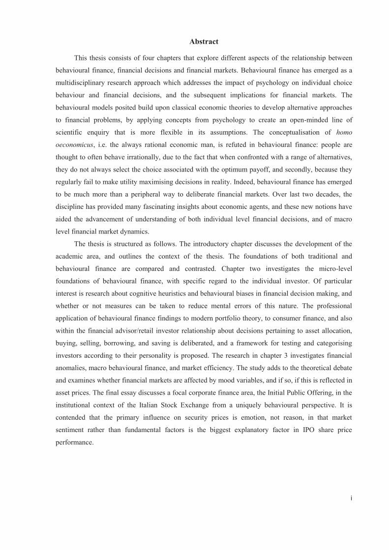
the fact that normal people are unable to ascertain relative qualities and probabilities accurately leads to
market outcome effects not predicted by the EMH. Hence, the manner in which agents form expectations
should be considered a crucial component of any model of financial markets. Prospect theory takes these
thoughts into consideration.
Figure 3: The Hypothetical Value function
(Source: Kahneman and Tversky, 1979)
Figure 4: The Hypothetical Weighting function (1979) and Weighting functions for gains (w+) and losses (w−)
(Source: Kahneman and Tversky, 1979 and 1992)
Later Tversky and Kahneman developed a new version of prospect theory, which they called
cumulative prospect theory (Figure 4 illustrates the weighting function in 1979, left hand side, and then
the newer version created in 1992 on the right hand side). In both versions, which were produced by way
of experiment, probabilities are replaced by decision weights and these decision weights are generally
lower than the corresponding probabilities, except in the range of low probabilities (Sewell, 2007). The
decision weight represents the impact of a given probability valuation of a prospect. It was empirically
found that people usually under weigh outcomes that are merely probable (low probabilities) in
comparison with outcomes that are obtained with certainty. Additionally, they under weigh med-high
probabilities. The newer version, based on median estimates of y and delta, employed cumulative rather

13
than separate decision weights.20 In addition the idea that cumulative weight can apply to uncertain as
well as to risky prospects with any number of outcomes allowing for different weighting functions for
gains and for losses was introduced. The 1992 theory envisaged a unique fourfold pattern of risk attitudes:
risk aversion for gains and risk seeking for losses of high probability; risk seeking for gains and risk
aversion for losses of low probability (Sewell, 2007).
2. Shifting Paradigm and the Philosophy of Science
“Directly testing the validity of a model’s assumptions is not common practice in economics, perhaps because of Milton Friedman’s influential argument that one should evaluate theories based on the validity of their predictions rather than the validity of their assumptions. Whether or not this is sound scientific practice, we note that much of the debate over the past 20 years has occurred precisely because the evidence has not been consistent with the theories, so it may be a good time to start worrying about the assumptions. If a theorist wants to claim that fact X can be explained by behaviour Y, it seems prudent to check whether people actually do Y”. Baberis and Thaler (2003; p.65)
It could be said that the underlying principles behind the philosophy of science are often overlooked
in the research of many academics within a diverse range of scholarly disciplines; no more so is this true
than in financial economics. The basic tenets of why academic research is conducted in the first place are
frequently brushed aside in favour of maintaining the pre-existing accepted generalizations about
economic phenomena. The status quo is preserved longer than it should be. As Thomas Kuhn the
American intellectual and philosopher posited, “Science undergoes periodic paradigm shifts instead of
progressing in a linear and continuous way” (Kuhn, 1996). Moreover, these paradigm shifts open up new
approaches to understanding that scientists would never have considered valid before. The legitimacy of
this statement is concrete and the vast majority of scientists would concur with Kuhn here.21 So, given
that there is much to be gained from scientific disunity and the subsequent paradigm shifts, it should be
useful to examine the potential benefits of a mixed disciplinary approach. From the previous section we
have seen that behavioural economics/finance was born out of the perceived doubts and qualms with
regard to the assumptions of modern neoclassical economics. It has been primarily informed by inputs
from psychology, and from behavioural decision research. In a Kuhnian sense, this new line of thinking
will hopefully be incorporated into a new paradigm which will add to the explanatory power of the
20 A related concept to value weighted theory is the notion of bounded rationality; which implies the retention of individual rationality but relaxation of the consistent beliefs assumption (investors don’t always apply Bayes Law in relation to probability). 21 The counter argument of this thought relates to the famous Charles Darwin saying “Natura non facit saltum”, which is Latin for "nature does not make jumps" – see Alfred Marshall, ‘Principles of Economics’ (1890) for more on this.

14
discipline. This would naturally imply that the basic object of study would have to be changed, which
entails that at a very abstract level, the central economic science axioms must be rethought also.22
An important question posed in the behavioural finance literature is whether economics is a positive
science. The quote above from Baberis and Thaler (2003) readdresses the fact that when discussing any
work within the extensive area of economics academia, it is worthy to reiterate that research can be
positive or normative in nature. Positive research (descriptive and explanatory enquiry) outlines what
economic agents actually do, while normative research stipulates what they should do. In other words,
positive research describes what is, whereas normative research prescribes what should be.23 Let’s take
the investment decision process for instance. Behavioural finance employs positive methods whereas
traditional economic analysis uses more normative methodologies; this key difference entails that BF can
provide more viable explanations about the missing gaps between what we ought do and what we do do.
In fact, the discrepancy between the normative traditional theories and behavioural descriptive models can
be construed to represent systematic irrationalities in human reasoning and cognitive abilities. In an ever
increasing number of empirically based studies in the heuristics and biases literature, which started in the
1970s and 1980s, it has been shown time and time again that individual behaviour strays from the
normative predictions (Stanovich and West, 2000). This division between the normative and the
descriptive is important as the traditional models can be maintained as the normative theory, while the
alternatives provided by behavioural models can be understood as descriptive theory. A prominent
example of this incongruence is the Allais Paradox (1953), which shows that choices regularly violate the
two foundational axioms of expected utility, the independence axiom and the sure-thing principle (Savage,
1954). The search for more realistic alternative assumptions to improve the predictive accuracy of an
economic model requires a testing of which factors make the biggest difference to the underlying variable
under observation: a theory ought to yield predictions about phenomena. For the test of realism,
methodological principles and an understanding of what features of the problem or of the circumstances
have the greatest effect on the accuracy of the predictions yielded by the particular theory are needed. A
key goal is the development of new assumptions that are more realistic as Herbert Simon argued that
Friedman’s idea of ‘Positive Economics’ is fundamentally flawed and that economists should directly test
economic model assumptions in addition to model implications: “In imagining that theories are used in
their simplest idealized form, ignoring real world complications, Friedman has drawn a fictitious picture
of how theories are actually employed in physical science and engineering, and given bad advice as to 22 As highlighted recently by Nobel Prize winner Joseph Stiglitz: “If science is defined by its ability to forecast the future, the failure of much of the economics profession to see the crisis coming should be a cause of great concern....economists must search for new paradigms” (Stiglitz, 2010; p.1). 23 This distinction has its roots in the fact-value distinction in philosophy, for more information in this area the reader is directed towards the work of Karl Popper.

15
how they should be employed in economics” (Simon, 1982; p.19). These apparent strengths lead to a
glaring weakness however: the reliance on traditional finance as a paradigm, and its increased intellectual
flexibility, makes it difficult to disprove and to validate some of the most prevalent behavioural models.
That being said, it is nigh on impossible to fully model every aspect of economic phenomena and human
economic behaviour as they are varied and complex, however that doesn’t entail that one should not
endeavour to do so.
In spite of the opinion expressed by Thaler (1999; p.12): “The controversy surrounding BF is dying
out as scholars accept it as simply a new way of doing economic research”, the battle between the
standard finance camp and other contrasting notions of finance that has raged on for the last two decades,
still continues. Thaler’s statement was made in 1999, however since then it is partly true that the
incorporation of psychology and finance has become more widely tolerated. Many new ideas have been
proffered and a plethora of articles have been written on the debate. Of these, a most famous input came
from Eugene Fama who described behavioural finance as “the anomalies literature” (1998). His
proclamation, at the time, was considered to be derogatory but it could now be deemed legitimate and
complimentary in another sense: the fact that Fama (being the spearhead of traditional finance academia)
dismissed such contrary work to the traditional/modern finance paradigm indicates that he felt that the
status quo was being threatened. What he was referring to was that much of BF is based on weak data and
evidence which was found using inaccurate methodologies. In truth this rebuttal is analogous to much of
the criticism of the discipline – detractors of behavioural economics/finance point to four explanations
which uphold the idea that human behaviour is largely rational and that the gap often found in studies
between rational economic predictions and actual behaviour is due to: performance errors, computational
limitations, the wrong norm being applied by the experimenter, and a different construal of the task by the
subject (Stanovich, 2000).
This denial of is course a common response to anomalies, however Fama’s assessment is incorrect
and calling BF the anomaly literature is a “means of discrediting” important evidence (Frankfurter and
McGoun, 2001). Furthermore, the majority of anomalies (which we will discuss more closely in a
proceeding ‘micro’ and ‘macro’ sections) have undergone rigorous data triangulation (Lucey, 2000).
Therefore, under the light of the scientific process, empirical falsification, and critical rationalism, which
strongly postulates that anomalies contribute significantly to the development of new and ultimately more
successful theories, these findings should not be dismissed. Anomalies can be scientifically significant as
the identification of departures, deviations, and discrepancies from existing theories helps in the
formulation of original improved theories. New and unexpected phenomena can often light the way for
future direction research; therefore if this is indeed the case, then different lines of enquiry and multi
perspective academic research in pursuit of better theories must be encouraged. However, even though

16
this may be so, it should also be remembered that a theory tends to be accepted not only due to the
empirical evidence/test but also because “researchers persuade one another that the theory is correct and
relevant” (Black, 1986; p.537).
3. Discussion The majority of observers would agree that the on-going global financial crisis which started in
2008 has once again highlighted the role of psychology in financial markets, and how susceptible they are
to asset price inflation, market instability, and indeed the overall welfare of society. For example, the sub-
prime mortgage debacle which occurred in the US presents a copious amount of proof of defective
consumer decision-making. In addition, few academics in traditional economics were able to foresee the
massive bubble and tremendous overvaluations which were developing in the US housing market; some
within behavioural finance did (such as Robert Shiller in 2005). With regard to individual investors in this
period, many of those who were deemed risk tolerant by their advisors had investment portfolios over-
weighted towards equity assets. However, once volatility in the markets increased many investors
panicked and sold at the market bottom. This behaviour, which was contrary to that envisioned by the risk
assessments used by the financial advisors to appraise and steer investors, has shown many of the classical
finance tools available to advisors to be lacking. From an ex-post perspective clearly many economic
predictions were disastrously wrong and the mainstream discipline was unable to predict the economic
dynamics of the phenomenon with such a small number of rules and laws. Overconfidence in the power of
traditional economic models that have been out of synch with real-world data, has been shown to be quite
dangerous. Evidence indicates that we depart from rationality in our economic decisions and behaviours in
predictable patterns, but what is required is a more sophisticated explanation of how emotions and relative
reason enable us to perform in the challenges we face. This undermining of homo oeconomicus (i.e. the
economic rational man who acts in his own self-interest and always maximises his own personal payoffs)
has many important consequences. These implications can assist policymakers recognising which
dynamics, apart from solely economic ones, may impact upon the financial behaviour of individuals and
markets. There are other crucial elements within financial economics, and understanding them is
elementarily important to the improvement of both financial market analysis and the formulation of
systemic risk presentation measures by governments.
As touched upon previously, the model most responsible for the emergence of behavioural finance
as a reputable academic area is Prospect Theory. Perhaps the most valuable aspect of prospect theory is
that it is construction model which wholly attempts to incorporate this facet of the human decision making
process into its thinking. Prospect Theory is undoubtedly an important basis of behavioural finance but we
need to ask ourselves whether it is justifiably so. Of course in absence of an alternative theory which can

17
better describe behaviour, decisions and risk attitudes, behavioural finance researchers have used this
model as a main foundation of thinking. To examine how psychology and economics has evolved, it is
evidently clear that the first behavioural economists considered that the mind is an ‘imperfect machine’ of
sorts. From this initial concept they then developed further models based upon the idea that this imperfect
machine is systematically encouraged into error by the duplication by psychological bias mechanisms and
cognitive heuristics (Frey and Stutzer, 2007), many of which will be detailed in chapter two. One main
reason as to why Prospect Theory has attained such approval and admiration is that it codifies these
irrational behavioural processes into a formal decision making model. The anomalies, cognitive heuristics,
emotional biases, psychological traps etc. are converted into more uniform and regular patterns of human
conduct. What’s more, this model has also enhanced our ability to make predictions about how people will
act in a given situation. On the other hand, one largely acknowledged criticism of this model of behaviour
is that it takes a ‘black box’ type approach in its thinking. That is to say it does not specifically consider
the inner workings and cognitive intricacies of the human brain. Prospect theory aims to predict behaviour
rather than to fully understand the mind’s internal processes that generate the behaviour – this perhaps is
where the research of another newer but fundamentally related field called neuroeconomics, which does
consider the internal processes, can be of most use into the future.

18
4. Bibliography
Ainslie, G. 1992, Picoeconomics: The Strategic Interaction of Successive Motivational States Within the Person, New York: Cambridge University Press.
Allais, M. 1953, Le Compartement de l’Homme Rational Devant le Risque, Critique des Postulates et Axiomes de l’Ecole Americaine, Econometrica, no. 21; pp.503-546.
Barberis, N. and Thaler, R.H. 2003, A Survey of Behavioural Finance, in Constantinides, G.M, Harris, M. and Stulz, R. eds., Handbook of the Economics of Finance. North Holland, Amsterdam.
Bell, D.E. 1982, Regret in decision making under uncertainty, Operations Research, Vol. 30, pp.961–981. Belsky, G. and Gilovich, T. 1999, Why Smart People Make Big Money Mistakes and how to correct them: lessons
from the new science of Behavioural Economics, Simon & Schuster: New York, ISBN: 0684844931 Bernoulli, D. 1738, Specimen Theoriae Novae de Mensura Sortis, Commentarri Academiae Scientiarum Imperialis
Petropolitanae, Tomus V, pp.175-92. Black, F. 1986, Noise, Journal of Finance, Vol. 41. No. 3, pp.529-543. Chew, S. H. and MacCrimmon, K.R. 1979, ‘Alpha utility theory, lottery composition and the Allais Paradox’,
University of British Columbia Faculty of Commerce and Business Administration, No. 686. Chew, S. H. and Epstein, L.G. 1989, The Structure of Preferences and Attitudes towards the Timing of the
Resolution of Uncertainty,International Economic Review, Vol. 30, pp.103 117. Dekel, E. 1986, Axiomatic Characterization of Preferences under Uncertainty: Weakening the Independence Axiom,
Journal of Economic Theory 40 304-318 DeBondt, W.F.M. and Thaler, R.H. 1985, Does the stock market overreact?, Journal of Finance, Vol.40, No.3,
pp.793-805. DeBondt, W.F.M. and Thaler, R.H. 1994, Financial Decision-Making in Markets and Firms: A Behavioural
Perspective, NBER Working Papers, 4777, National Bureau of Economic Research, Inc. Edgeworth, F.Y. 1881. Mathematical Psychics: An Essay on the Application of Mathematics to the Moral Sciences,
Publisher: C.K. Paul, London. Elton, E.J. and Gruber, M.J. 1995, Modern portfolio theory and investment analysis, New York: Wiley ISBN: 978-
0470388327. Fama, E.F. 1965, The Behaviour of Stock-Market Prices, Journal of Business, vol. 38, no. 1, pp.34-105. Fama, E.F. 1970, Efficient Capital Markets: A Review of Theory and Empirical Work, Journal of Finance, vol. 25,
no. 2, pp.383-417. Fox C.R 2006, Neuroeconomics: Week 4 Decision Under Risk, UCLA Seminar, available for download
at:www.poldracklab.org/.../neuroeconomics/neuroec-week4-5-risk-uncert.ppt Fox, C.R., & Tversky, A. 1995, Ambiguity Aversion and Comparative Ignorance, The Quarterly Journal of
Economics, Vol. 110, No. 3. Aug., 1995; pp.585-603. Frankfurter, G.M., McGoun, E.G and Allen, D.E, 2004, The prescriptive turn in behavioural finance, Journal of
Socio-Economics, Vol. 33, pp.449-468. Frankfurter, G. M. and McGoun, E. G. 2001, Anomalies in Finance: What Are They and What Are They Good For?,
International Review of Financial Analysis, Vol. 10, No. 4, pp.407 429. Frey, B.S. and Stutzer, A. 2002, What Can Economists Learn from Happiness Research?, Journal of Economic
Literature, Vol. 40, pp.402-35. Friedman, M. and Savage, L.J. 1948, Utility Analysis of Choices Involving Risk, Journal of Political Economy, Vol.
56, No. 4, pp.279–304. Friedman, M. 1953, Essays in Positive Economics, University of Chicago Press Fuller, R.J. 1998. Behavioural Finance and the Sources of Alpha, Journal of Pension Plan Investing, Winter, Vol. 2,
No. 3. Gigerenzer, G. 1993, From metaphysics to psychophysics and statistics, The Behavioural and Brain Sciences, 161,
139-140. Glimcher, P.W. 2003, Decisions, uncertainty, and the brain: The science of neuroeconomics, Cambridge, MA: MIT
Press. Grinblatt, M. and Keloharju, M. 2001, What Makes Investors Trade?, The Journal of Finance, Vol. 56, pp.589-616. Gul, F. 1991, A theory of disappointment aversion, Econometrica, Vol. 59, pp.667-686. Hands, D.W. 2010, Economics, Psychology, and the History of Consumer Choice Theory, Cambridge Journal of
Economics, Vol. 34, no. 4, pp.633-648. Heukelom, F. 2007, Kahneman and Tversky and the Origin of Behavioural Economics, Tinbergen Institute
Discussion Paper, TI 2007-003/1, available at. http://www.tinbergen.nl.

19
Hicks, J.R. 1939, Value and Capital: An Inquiry into Some Fundamental Principles of Economic Theory, Oxford: Clarendon Press.
Jallais, S., and Pradier, P.C., 2005, The Allais Paradox and Its Immediate Consequences for Expected Utility Theory, in P. Fontaine and R. Leonard eds, The Experiment in the History of Economics, London: Routledge, pp.25-49.
Jones, B.D, 1999, Bounded Rationality, Annual Review Political Science, Vol. 2, pp.297-321. Kahneman, D. 2003, A Psychological Perspective on Economics, American Economic Review, Vol. 93, pp.162-68. Kahneman, D. and Frederick, S. 2002, Representativeness Revisited: Attribute Substitution in Intuitive Judgment, in
Gilovich, T., Griffin, D. and Kahneman, D. eds, Heuristics and Biases: The Psychology of Intuitive Judgment pp.49-81, New York: Cambridge Uni Press.
Kahneman, D., Knetsch, J.L. and Thaler, R.H. 1991, The Endowment Effect, Loss Aversion, and Status Quo Bias: Anomalies, Journal of Economic Perspectives, Vol. 5, no. 1, pp.193–206.
Kahneman, D. and Thaler, R.H. 1991, Economic Analysis and the Psychology of Utility: Applications to Compensation Policy, The American Economic Review, Vol. 812, pp.341-346.
Kahneman, D. and Sugden, R. 2005. Experienced Utility as a Standard of Policy Evaluation. Environmental & Resource Economics, 32, 161-181.
Kahneman, D. and Tversky, A 1992, Advances in Prospect theory: Cumulative Representation of Uncertainty, Journal of Risk and Uncertainty, Vol. 5, no. 4.
Kahneman, D. and Tversky, A. 1972. Subjective Probability: A Judgment of Representativeness, Cognitive Psychology, Vol. 3, pp.430-454.
Kahneman, D. and Tversky, A. 1973, On the Psychology of Prediction. Psychological Review, vol. 80, pp.237-251. Kahneman, D. and Tversky, A. 1979, Prospect Theory: An Analysis of Decision under Risk, Econometrica, vol. 47,
pp.313-327. Kahneman, D., Walker, P. and Sarin, R. 1997. Back to Bentham? Explorations of Experienced Utility. The Quarterly
Journal of Economics, Vol. 112, No.2, pp.375-405. Keynes, J.M. 1936, The General Theory of Employment, Interest, and Money, London: Macmillan. Kuhn. T. 1996, The structure of scientific revolutions, 3rded., Chicago: University of Chicago Press. Laibson, D. 1997, Golden Eggs and Hyperbolic Discounting, Quarterly Journal of Economics, Vol. 112, pp.443–
477. Laing, G.K. 2010, Impact of Cognitive Biases on Decision Making by Financial Planners: Sunk Cost, Framing and
Problem Space, International Journal of Economics and Finance, Vol. 2, No. 1. Lamont, O.A. and Thaler, R.H. 2003, Can the market add and subtract? Mispricing in tech stock carve-outs, Journal of Political Economy, Vol. 111, pp.227-268. Larrick, R.P. 2004, Debiasing, Chapter 16 in Blackwell Handbook of Judgment and Decision Making, Koehler, D.J.
and Harvey, N. Eds., Blackwell Publishing Ltd. List, J. A. and Haigh, M.S. 2005, A simple test of expected utility theory using professional traders, Proceedings of
the National Academy of Sciences, January, Vol. 102, no. 3, pp.945–948. Lintner, J. 1965 The valuation of risk assets and selection of risky investments in stock portfolios and capital
budgets, Review of Economics and Statistics, Vol.47, pp.13-37. Lo, A.W. and Mueller, M.T. 2010, Warning: Physics Envy May be Hazardous to Your Wealth!, Available at SSRN:
http://ssrn.com/abstract=1563882 Loewenstein, G. 1992 The Fall and Rise of Psychological Explanations in the Economics of Intertemporal Choice, In
Choice Over Time, Loewenstein, George and Jon Elster, ed. New York: Russell Sage Foundation, pp.3–34 Loewenstein, G., and Prelec, D. 1992, Anomalies in Intertemporal Choice: Evidence and an Interpretation, Quarterly
Journal of Economics, Vol.107, pp.573–597. Lucey, B. 2000, Friday the 13th and the Philosophical Basis of Financial Economics, Journal of Economics and
Finance, Vol. 24, No. 3, Fall, pp.294-301. MacKay. C. 1841, Extraordinary Popular Delusions And The Madness Of Crowds, Harriman House Limited. Marshall, A. 1890, Principles of Economics, Publisher, London: Macmillan and Co. Markowitz, H. 2005,Market Efficiency: A Theoretical Distinction and So What?, Financial Analysts Journal, Vol.
61, No. 5, pp.17-30, September/October Neumann, J. V., and Morgenstern, O. 1944, Theory of Games and Economic Behaviour, Princeton: Princeton
University Press. Odean, T. 1998, Are Investors Reluctant to Realize Their Losses?, The Journal of Finance, Vol.53, no.5,pp.1775-
1798. Quiggin, J. 1982, A theory of anticipated utility, Journal of Economic Behaviour& Organization, Vol. 3,
pp.323 343.

20
Rabin, M. 1998, Psychology and Economics, Journal of Economic Literature, Vol. 36, pp.11-46. Ritter, J. 2003, Behavioural Finance, Pacific-Basin Finance Journal, Vol. 11, No. 4, September; pp.429-437. Sanfey, A.G., Rilling, J.K., Aronson, J.A., Nystrom, L.E., and Cohen, J.D. 2003, The neural basis of economic
decision-making in the Ultimatum Game, Science, Vol. 300, pp.1755–1758. Samuelson, P.A. 1938, A Note on the Pure Theory of Consumer's Behaviour, Economica, Vol. 5, pp.61-71. Robbins, L. 1952, An Essay on the Nature and Significance of Economic Science, 2nd edition, London: Macmillan,
first edition published in1932. Savage, L. J. 1954, The foundations of statistics, John Wiley & Sons Inc., New York. Schoemaker, P. 1982, The expected utility model: its variants, purposes, evidence and limitations, Journal of
Economic Literature, Vol. 20 June, pp.529-563. Segal U. 1989, Anticipated Utility. A Measure Representation Approach, Annals of operations Research, Vol.19,
pp.359-373. Sent, E.M. 2004, Behavioural Economics: How psychology made its limited way back into economics, History of
Political Economy, Vol. 364, pp.735-760. Sewell, M. 2007, An Introduction: Behavioural Finance, University College London, available at
http://www.cs.ucl.ac.uk/staff/M.Sewell/publications.html Schwartz, H.H. 2007, An Introduction to Behavioural Economics: The Complicating but Sometimes Critical
Considerations, Available at SSRN: http://ssrn.com/abstract=960222 Sharpe, W.F. 1964, Capital Asset Prices: A Theory of Market Equilibrium under Conditions of Risk, Journal of
Finance. Vol.19, No. 3, pp.425–442. Shiller, R.J. 2005, Irrational Exuberance, Second Edition, Princeton University Press. Simon, H.A. 1955, A Behavioural Model of Rational Choice, Quarterly Journal of Economics, 69; pp.99-118. Simon, H.A. 1982, Models of bounded rationality 2 vols., Cambridge, MA: MIT Press. Simon, H.A. 1987., Rational Decision Making in Business Organisations, in Advances in Behavioural Economics:
Vol. 1, ed. L. Green and J. H. Kagel, 18–47. Norwood, NJ: Ablex. Simonson, I. and Tversky, A. 1992, Choice in Context: Trade-off Contrast and Extremeness Aversion, Journal of
Marketing Research, Vol. 293, pp.281-295. Slutsky, Eugene E. 1915, Sulla Teoria del Bilancio del Consonatore, Giornale degli Economisti, Vol. 51, pp.1-26, the
translated version in appeared Readings in Price Theory, G. J. Stigler and K. E. Boulding eds., Homewood, IL: R.D. Irwin, 1952, pp.27-56.
Smith, A. 1776, An Inquiry into the Nature and Causes of the Wealth of Nations, London: Methuen & Co., Ltd. Stanovich, K. E. 1999, Who is Rational? Studies of Individual Differences in Reasoning, Mahwah, NJ: Erlbaum. Stanovich, K.E. and West, R. 2000, Individual difference in reasoning: implications for the rationality debate?,
Behavioural and Brain Sciences, no. 23, pp.645–726. Statman, M. 1999, Behavioural Finance: Past Battles and Future Engagements, Financial Analysts Journal,
Association for Investment Management and Research, November/December 1999. Stiglitz, J. 2010, Needed: a new economic paradigm, August 19th 2010, online article available for download at
http://www.ft.com/cms/s/0/d5108f90-abc2-11df-9f0200144feabdc0.html#axzz16Iah8D1R. Stracca, L. 2004, Behavioural finance and asset prices: Where do we stand?, Journal of Economic Psychology, Vol.
25, pp.373–405. Thaler, R.H. 1992, The Winner’s Curse: Paradoxes and Anomalies of Economic Life, NJ: Princeton University Press. Thaler, R.H. 1993, Advances in Behavioural Finance, Vol. I Edition, New York: Russell Sage Foundation. Thaler, R.H. 1999, The End of Behavioural Finance, Financial Analysts Journal, Vol. 56, No. 6, pp.12-17. Thaler, R.H. 2000, From Homo Economicus to Homo Sapiens, Journal of Economic Perspectives, Vol. 14, pp.133–
141. Thaler, R.H. 2005, Advances in Behavioural Finance, Vol. II Edition, NJ: Princeton University Press. Thaler, R., Mullainathan, S. and Kahneman, D. 2008, A Short Course In Behavioural Economics, Edge Masterclass,
Sonoma, California USA, July 25-27. Tversky, A., and Kahneman, D. 1981, The Framing of Decisions and the Psychology of Choice, Science, Vol.
211,No. 4481, pp.453–458. Tversky, A., and Kahneman, D. 1986, Rational Choice and the Framing of Decisions, The Journal of Business, 59,
No.4, pp.251-278. Von Neumann, J. and Morgenstern, O. 1944, Theory of Games and Economic Behaviour, Princeton University. Whalley, J. 2004, Rationality, Irrationality and Economic Cognition, The University of Western Ontario, Peking
University and NBER, CSGR Working Paper, No. 145/04. Websites: www.economist.com/PrinterFriendly.cfm?Story_ID=382968

21
Chapter 2. BF Micro: Individual level
1. Introduction
As discussed in the first chapter of this thesis, much of the chaotic behaviour seen in financial
markets does not make sense conceptually using modern financial theory. A multitude of
discrepancies between actual responses in financial markets and those dictated by normative models
have been documented – individuals have been found to violate the axioms of utility theory in the way
that they behave, financial markets have often been shown to be inefficient and a range of anomalous
phenomena has been recorded. Alternatively, thinking from a more descriptive behavioural viewpoint
has grown in recent years to increase understanding of economics and financial market outcomes. By
extension of the same principles to the micro individual level, behavioural finance has also sought to
explain why and how people make “seemingly irrational or illogical decisions when they spend,
invest, save, and borrow money” (Belsky and Gilovich, 1999; p.2). Financial decision making
involves strong emotional processes and hence behavioural economists have used concepts from
psychology to better understand the patterns regarding how people behave. Research has dealt with
important issues such as the causes behind why people regularly make flawed decisions with money,
and how investors’ actions often conflict with those depicted by the paradigm of rational decision
making and traditional portfolio choice theories; the heuristics and biases research program has
become particularly important in increasing understanding of individual and market behaviour. As a
consequence of heuristics/biases, various negative outcomes can result, like the inappropriate and
often hazardous purchase of financial products by consumers, ill-advised buying and selling decisions,
under saving for retirement, insufficient portfolio diversification and reduced financial well-being. For
example, retail investors in financial markets, who exhibit strong overconfidence bias, i.e. they over-
rate their own abilities, tend to hold riskier portfolios and over-trade to the detriment of their wealth –
this is not the behaviour of a utility maximiser (Odean, 1998).
The question posed in this paper is how behavioural finance findings can be actively applied to
areas such as in the financial advisor client relationship. Motivation for the paper is grounded in the
fact that a gap exists in the literature: behavioural finance has pointed out the weaknesses and failings
of traditional rational models without being able to concretely offer a practical alternative which can
be used in professional settings. Research has focused on demonstrating in what ways we go wrong
rather than detailing how the problems can be avoided or fixed. In actual fact, a popular phrase
repeated in many articles relating to biases is often along the lines of “here we have listed some of the
most prevalent mental biases and we hope that recognising these will help you avoid these pitfalls in
the future”. In this paper I aim to investigate some of the possible ways in which micro-behavioural

22
finance research can be applied to the real world. Through the application of psychology and utilising
learning from other behavioural sciences, micro BF helps to overcome the shortcomings of the
traditional finance approach. The plan of the paper is as follows. Section 2 starts with an overview of
the various mental errors that provide the basis for much of the behavioural finance literature. Section
3 investigates the ways in which behavioural finance concepts can be applied in a practical sense.
Section 4 of the paper examines the link between finance and personality. The paper ends with a
discussion and synopsis of the paper’s major arguments.
2. The Behavioural Biases which affect Financial Decisions
2.1. Financial Decision Making
“To make a decision, emotion is the necessary trigger and without emotion, one would be reduced to the state of an idiot savant who goes on endlessly calculating without the ability to make a choice” (Olsen, 2008; p.3)
A logical starting point for this section is a brief discussion of financial decision making.
Decisions about money and finance are made by various actors in the financial sector from individual
retail investors, families, corporate managers, businesses of all sizes, governments, institutional
investors, professional investors, financial advisors, traders, brokers, dealers, and fund managers. For
instance, throughout their lives individual retail investors will make a wide range of different decisions
(saving, investing, buying, selling and holding) with regard to their own personal finances: where to
deposit savings, how much and when money will be needed to cover current/future consumption
needs, which banking institution to use for day to day transactions, how to pay for their children’s
education, how to arrange home equity loans, whether or not to use credit borrowing for items such as
car purchases and which investments will cater for the highest standard of living for the retirement
years. On the other hand, financial advisors and asset/fund managers act as agents as they are
responsible for making important decisions about other people’s money (e.g. pension funds) on a
frequent basis; they must decide which assets to buy (selection), how much of the portfolio to allocate
(weighting) and when to sell or unwind certain positions.
Decision making is a complex and cross disciplinary area that is particularly germane to
finance.1 The behavioural view and classical view of financial decision making differ in several key
ways. First of all from the classical perspective, decision making theory is based upon expected utility
1 An initial distinction must be made between those decisions requiring cognitive mechanisms which are automatic in their operation, accepting no input from deliberative or effortful processes, and more complicated decisions that employ cognitive mechanisms which require deliberative and conscious processes (Barrett et al., 2006) – this dual process system will be discussed in greater detail in the subsequent section.

23
and is concerned with goal-directed behaviour in the presence of options (Hansson, 1994). It is used to
find optimal solutions in circumstances where a decision maker has to analyse several alternatives
with risk probabilities attached to each before selecting a choice. There are four fundamental elements:
acts, events, outcomes and payoffs. Acts are the alternative actions (options) available for
consideration to the decision maker. Events are occurrences which take place outside the control of the
agent. Outcomes are the product of the occurrence of acts and events. Payoffs are the values the
decision maker is placing on the occurrences – payoffs may be positive or negative (Lapin and
Whisler, 2001). When confronted with the alternative acts, economic agents in the classical model are
thought to decide which is best by applying concepts from the work of Von Neumann and
Morgenstern (1944) on utility. Their model outlines that when a rational decision making procedure is
employed, numbers representing personal values for the alternative outcomes can be derived. When
probabilities of the events are not known, several approaches are available for an agent to use in
developing a criterion to base the choice on. The maximax approach is optimistic and stipulates that
the act with the largest possible outcome is chosen. The conservative maximin approach chooses the
act with the largest minimum payoff: this means that the decision maker is guaranteed to do no worse
than the best of the poorest outcomes. The minimax regret approach involves taking the maximum
payoffs of each event and subtracting the outcome from each event from this maximum payoff. The
act with the smallest maximum regret is then chosen.
Decision approaches are different for situations where probabilities are known and the
probabilities of each event vary (i.e. there is risk of both a positive or negative outcome involved).
Under Maximum Likelihood Decision Making the choice criterion is that the alternative associated
with the most likely event is optimal – the other events and outcomes are excluded and ignored. Using
Bayes’ Decision Rule, the act (the choice or bet made) which maximises the expected payoff (EMP)
is the optimum choice, as it has the highest probability-weighted payoff associated with it. Selection
amongst alternatives with probability and risks attached to them is based upon the size of their
expected utility values (Oliveira, 2007).
Contrastingly, a behavioural finance view of the financial decision-making process (Redhead,
2008) differs from the classical view in several key aspects. Firstly, decision making from the
behavioural perspective relaxes some of key assumptions of the classical model. The Bayes Decision
rule that is so central to traditional finance theory, does have the advantage in that it makes the greatest
use of all available information. If alternative ‘X’ has a higher expected utility than that of ‘Y’ then it
should always be selected. However, it is assumed that the agent is indifferent to risk, and problems
may arise when the alternatives involve different magnitudes of risk – if option ‘X’ has a higher utility
due to high risk but high possible payoff also, taking that high risk gamble may not be the best choice

24
available in reality due to other considerations. Studies in finance deal with decision making under risk
often on the basis of stochastic financial data such as asset price returns (Wu et al., 2005). In
behavioural finance a main assumption is that choice may not be the outcome of a utility maximisation
process; this directly contrasts with traditional finance. Relating to money specifically, sound financial
decision-making is based upon performing a logical cost benefit analysis and a crucial element of such
a cost benefit analysis is determining the value of money over time. However, about issues such as
pension structure saving and for retirement for instance, it has been found that individuals make
flawed decisions consistently due to a lack of self-control, limited information, time, and cognitive
ability (Mitchell and Utkus, 2003). People are often not able to make decisions which are in their own
long term financial interest. One example which highlights this problem well comes from Elan and
Goodrich (2010) who examine an individual’s propensity to choose whether to save or not; in other
words deferring consumption. The study shows that this propensity is dependent on the subjective
discount rate applied to the time value of money: ‘exponential discounters’ have a greater propensity
to save more as they attach higher value to future money than ‘hyperbolic discounters’.
A second difference relates to how information is dealt with. In finance, objective information
which may come in the form of historical prices, public information, private information, or noise is
selected and interpreted. However, in the behavioural model, information overload during the
perception stage could terminate the process. Next when the information comes to be processed, the
behavioural model incorporates the fact that humans will often employ ‘satisficing’ subject to heuristic
simplification, self-deception, social influences, emotion, and mood. The decision to buy, sell, or hold
is then deliberated. However, instead of being acted upon at once, the decision may be hampered by
procrastination or inhibition before it is actually implemented.
2.2. Decision Heuristics and Cognitive Biases
“In summary people trade for both cognitive and emotional reasons: they trade because they think they have information when they have nothing but noise, and they trade because trading can bring the joy of pride. Trading brings pride when decisions turn out well, but it brings regret when decisions do not turn out well. Investors try to avoid the pain of regret by avoiding the realisation of losses, employing investment advisors, and avoiding stocks of companies with low reputations” (Statman, 1988; p.30)
In the majority of the financial decisions, such as financial asset trading mentioned in the quote
above by Statman (1988), a plethora of behavioural biases which afflict human behaviour have been
found. The fact that human nature causes investors to fall prey to biases distinguishes them from the
rational actors depicted in classical economic theory. Furthermore, empirical research has shown that
professional investors as well as private retail investors, are effected by irrational biases in their
investment decisions (e.g. Glaser et al. 2005; Haigh and List, 2005; Menkhoff et al. 2006). Thus, a

25
central goal in which BF strives for involves in analysis at the micro-scale, is to increase our
understanding of how individuals make decisions, form expectations, react to risk, how certain groups
of financial market participants behave, what kinds of portfolios they choose to hold and how they
should trade over time (Olsen, 2008). To achieve this, some of the restrictive assumptions of
traditional economics are loosened to take into account how real heterogenic economic agents make
decisions, and how they evaluate the desirability of alternative choices and then select a particular
option.
Behavioural finance research from the likes of Richard Thaler, Robert Shiller, and Daniel
Kahneman amongst others has shown over the last three decades that economic agents and financial
markets are not rational. Humans are not as smart as standard economic theory would have us believe
and as Kahneman summarised in his Nobel Prize Lecture (2002): “The mind is a system of jumps to
conclusions”. In light of these findings, much value can be obtained from investigating whether
incorporating behavioural based preference patterns has substantial influence on investor's optimal
behaviour. Additionally, and more damning of the rationality view of economic agents, is that people
seldom adhere to the logical models of choice, which suggests that variations in human behaviour
might not find any theoretical basis in normative models (Hoch et al., 2001). Humans don’t always
behave according to the assumptions of utility theory in that they do not search to identify all possible
outcomes, they are not always able to assign accurate probabilities to these outcomes, and they are not
able to unfailingly pick the best payoff from the options considered (Isenberg, 1989). According to
normative decision theory, such as Savage’s (1954) subjective expected utility (SEU), when decision
makers rank one alternative above another they would tend to rank them identically in other occasions
in which these possible choices would be available. However, agents often change preferences in front
of different framing of the same information (Tversky and Kahneman, 1981).
As previously discussed in the introductory chapter, the behavioural approach towards financial
decision making comes from the basic perspective that individuals have a bounded rationality in their
ability to make optimal judgments and choices at all times. Two consequences of this bounded
rationality are decision heuristics and cognitive biases. Results from psychology research, have
indicated that the information processing capacity of individuals is quite often weak; many
psychological phenomena, heuristics and biases are employed when people perform a variety of
complex tasks (Newell and Simon, 1972). The main determinants of many of these biases are
cognitive limitations in perception (Miller, 1956), attention (Kahneman, 1973), memory (Baddeley,
1986) and analytical processing (Simon, 1955). These limitations sharply constrain our ability to make
accurate judgments and to simultaneously consider multiple decisions. One must remember however
that, as argued by Binmore (1994; 1999) the anomalous behaviour can only be deemed economically

26
meaningful if it persists in an environment where individuals repeatedly face the same decision
problems and receive feedback on the outcomes of their decisions. Indeed, the heuristics and biases
unearthed have proven to be pertinent according to this measure, and the area has emerged as a main
paradigm in the psychology of judgment and decision making (Gilovich et al. 2002, Kahneman et al.
1982). A heuristic can be defined as a mental process which “tends to produce efficient solutions to
difficult problems by restricting the search through the space of possible solutions; the restriction on
search is based on evaluation of the structure of the problem” (Braunstein, 1976). It is a type of
prepared problem-solving aptitude and mental shortcut that is used in intuitive judgments of
probability, and to determine the solution to a given problem or make a decision.
Relative to the majority of other animals, the human brain receives a massive amount of
inbound sensory data when it is confronted with a given problem to solve (Shulz and Fregnac, 2010).
The brain detects changes in the environment and then packages the relevant data in an efficient
manner. Much of the data is instantly ignored. Precise compression schemes are used to filter the data
and only a very small percentage of it will be converted into relevant information (Maguire and
Maguire, 2010; Alvager, 1998). Beliefs about the probability that an event will occur are then
developed based upon this information, and the possible event outcomes and their respective payoffs
will be uncertain in nature. Assessing the probabilities and predicting values are complex tasks that are
transformed to simpler judgmental operations (Kahneman, Slovic, and Tversky, 1982). In this process,
the human brain makes associations with previous experiences that are archived in our long-term
memory. However, errors and certain biasing effects often arise as the compression schemes are not
perfect, and because our memory has limited capacity and duration.
Heuristics, which emanate from the complex associative network that is the human brain, are
fast, informal and intuitive ways of thinking that we use in abstract reasoning to produce a rough
answer to a question. In the main, heuristics are valuable as they allow us to make sense of
complicated situations quickly and enable us to make correct decisions under uncertainty. The human
brain uses them to make our lives easier, through clustering data, and by forming habits and patterns.
Heuristics in effect preserve brain processing power by reducing the information searching costs, time
and energy used up in making a decision. In this way heuristic rules act to keep the information
processing demands of a task within the bounds of the individual’s limited cognitive capacity
(Kahneman and Tversky, 1973). Sometimes a misdirection results however, and the ensuing judgment
of the surrounding environment is less than perfect. In effect, a disparity occurs between the reality of
the situation and the mental deduction made.
The constraints of our mental deduction system lead to heuristics, which in turn produce what is
known as cognitive biases. The failure to generate proper reasoning is the cause of cognitive biases,

27
which are “mental errors caused by our simplified information processing strategies” (Heuer, 1999;
p.111) and the tendency to make an incorrect deduction in a certain circumstance based on cognitive
factors. A bias can be thought of as an application of a heuristic. As a bias predominantly emanates
from a heuristic, many of the biases documented are related to each other (Kahneman and Frederick,
2002; 2005).
2.3. Investment Heuristics and Biases
What heuristic ‘shortcuts’ and biases do investors use in making decisions with money? Decision biases influence the way in which decision makers obtain, process, and assess information on which they construct their choices (Hogarth, 1987). They will undoubtedly play a large role in financial decisions. The empirical work in this area has been conducted in a wide range of contexts, from trading floors to laboratory settings. Although, as the same mental processes are employed there is no reason to think that biases would be domain specific (DeMeza, Irlenbusch, and Reyniers, 2008). Evidence has been presented which shows that consumers (Payne, 1976), but also investors of all kinds (DeBondt, 1998) are prone to biased decision making and heuristic cognitive processes. For example, choosing to invest at the wrong time is a regular occurrence for individual participants in financial markets (especially the equity market) – many investors follow the herd by buying at the peak and then proceed to panic sell at the market bottom. Recent examples include the internet bubble in 1999, the bursting of the USA housing bubble which occurred in 2007, and the flight of capital from equity markets in Europe throughout 2012.
The main investor heuristics biases and psychological traps documented in the behavioural finance literature are listed below (collated from Staw, 1976 and 1981; Samuelson and Zeckhauser, 1988; Hammond, Keeney and Raiffa, 1998; Pompian and Longo, 2005; Ware, 2008). To organize the many biases which have been registered, academics have used different categorisation methods. A key distinction, which is echoed throughout the behavioural finance literature, lies between the two major bias archetypes: emotional and cognitive.

28
Figure 1: Twenty of the Most Common Investment Heuristics and Biases
Emotional Cognitive
Endowment: Higher value placed on objects owned than on objects not owned. Overvalue own investments regardless of expected outcome.
Representativeness: Let pre-existing ideas influence how new information is processed. Distorting reality due to mind’s tendency to create patterns; conjunction fallacy.
Loss Aversion: The pain of losses is felt more acutely (twice as strong) than the pleasure of gains, leading to overly conservative behaviour.
Anchoring: The tendency to cling to previous information, such as arbitrary pricing levels when considering a decision, such as an investment.
Inertia and Status Quo: Decision-makers choose option that will keep conditions as they are. Bias toward alternatives that keep the current state.
Mental Accounting: Sums of money are categorised, not as one big pot but as separate buckets, which are treated differently.
Regret: Avoid making a decision because of fear of poor results: taking action and losing feels worse than doing nothing and losing (decision paralysis). Rationalising decisions to avoid negative feelings.
Recency: Overemphasis is placed upon events that are most recent.
Optimism: Investors believe that bad events can happen only to others, wishful thinking.
Hindsight: Investor perceives that an event was predictable, even when it wasn’t – rewriting history to suit a current preference, decision or choice.
Over-Confidence: Investor overestimates own skills and abilities. Failure is attributed to bad luck whilst success is due to skill.
Framing: Bias created in how data are presented with relation to reference points; the context in which the choice is presented unduly influences the decision.
Self-Attribution: Failure is attributed to bad luck whilst success is credited to innate skill.
Cognitive Dissonance: Rationalise a poor decision; distort reality based on need for internal harmony.
Self-Control: Investor spends today at the expense of saving for tomorrow.
Ambiguity Aversion: Preference for ambiguity-free options even when they seem less likely to succeed; stick with the ‘known’ to avoid uncertainty and chaos.
Conservatism: Investor sticks to initial view or forecast despite new information. Availability: Estimate probability of outcome based on the ease of obtaining the information, and the familiarity and prevalence of it. Confirmation: Selective screening and seeking out data to fit the existing position or point of view, whilst avoiding information that undercuts position. Tendency to favour information that affirms already-held beliefs. Illusion of Control Bias: The subject believes that they can control, or at least influence, investment outcomes when, in fact, they cannot.
It suffices to say that there are certain conditions whereby particular biases have a higher
likelihood of appearing. Most of the biases listed in figure 1 above occur before or during the making
of a decision, apart from the confirmation, hindsight and the endowment biases which are committed
after making a decision (Kahneman, Knetsch, and Thaler 1990). Categorisation of these phenomena
has also been conducted by Stracca in 2004. He sorts the most common behavioural biases and
psychological traps into 5 different categories, some of which overlap. The first category is that of
decision heuristics, discussed above, which involve economic agents who make use of shortcuts and

29
simple rules of thumb in making decisions, because they do not (and cannot) solve the (complex)
utility maximisation problems mainly reflecting deliberation and optimization costs (Colisk, 1996).
The second category of biases arises due to the interference of emotions and ‘visceral factors’ in
decisions (Loewenstein, 2000). Choice bracketing is the third category that includes biases regarding
to the way that agents tend to frame decision problems more narrowly than depicted in mainstream
economics (Read, Lowenstein, and Rabin, 1999). The example given in Stracca (2004) is that agents
normally have a shorter time horizon than their lifetime in their decisions. The fourth category is based
upon how individuals exhibit stochastic and context-dependent preferences.
Recent contributions claim that a set of well-defined and deterministic preferences, as the utility
function which is maximised, does not exist altogether. Rather, stochastic and context-dependent
preferences should be considered (Loomes and Sugden, 1995). The final category of biases materialise
due to the usage of reference dependent models. Agents’ preferences for consumption and other
variables (including risk) do not seem to be defined in abstract and general terms as in the standard
approach; rather, they depend on “reference points”. So, the utility function is not defined simply over
ct, but rather on ct - zt, where z is a reference point for the representative agent. One prominent
example of a model taking into account reference dependence is Prospect Theory by Kahneman and
Tversky (1979) which was discussed in the first chapter.
Biases have also been stratified by Virine and Trumper (2008) who group the biases according
to those related to perception (bias blind spot, inertia, illusion of control), biases related to prospect
theory (loss aversion, disposition effect, endowment effect),2 biases relating to estimation of
probability and belief (anchoring, ambiguity, optimism, availability, representativeness), biases which
are social or group based (attribution, groupthink), and memory biases and effects (hindsight). In a
similar manner to Stracca (2004), Lovallo and Sibony (2010) organise behavioural biases according to
five categories that have negative effects for decisions and the planning process. Biases are divided on
the basis of the shared traits inherent in each. Pattern recognition biases involve the misinterpretation
of conceptual relationships or identification of patterns where there are in fact none. Action-orientated
biases relate to the drive to take action too quickly. Stability biases materialise due to the tendency
toward inertia in the presence of uncertainty. Interest biases arise in the presence of conflicting
2 A related and causal aspect in loss aversion is the endowment effect, which was first identified by Thaler (1980) and then later studied by, amongst others, Kahneman, Knetsch and Thaler (1991); Kahneman and Tversky (1992). It basically implies that when a person comes into possession of a good he/she automatically ascribes to it a value which is higher than the value which existed before the property was possessed. People therefore demand considerably more to give up an object they own than they would be willing to pay to buy it. The endowment effect consequently is a contributing factor in loss aversion, which as we have discussed leads people to give more weight to a loss than to a foregone gain.

30
incentives (including non-monetary and even purely emotional ones). Finally, social biases are
founded on humans’ natural preference for harmony over conflict.
One micro anomaly in which we have yet to discuss that is particularly relevant to micro
behavioural finance is the ‘disposition effect’. The work of Daniel Kahneman and Amos Tversky
(1979) on prospect theory – the main insight of which is that pain felt from a loss is about two times as
strong as the feeling associated with realisation of a gain – is a key construct of behavioural finance
that has been fundamental in the development of some of the field’s cornerstone concepts. An example
of a resulting discovery based on the application of this prospect theory to investments is the
aforementioned disposition effect. Shefrin and Statman (1985) developed the term and summarised it
in the phrase as the tendency to “sell winners too early, and ride losers too long” (p.778). A person
can act conservatively when protecting gains (selling winners too soon to realise a profit) but quite
rashly by holding onto investments that have dropped in value for too long (in the hope that the share
will rebound to a breakeven value)3. This apparently irrational preference has been referred to as a
way in which humans seek to avoid regret (Barber and Odean, 1999). For instance, often what
happens is that investors grow attached to a specific company’s share and when it starts to fall in
value, the investor usually doesn’t want to sell and realise the loss. Conversely, the desire to
experience the pleasure from realising a gain makes investors sell the asset too soon. This is especially
true if the stock has been performing poorly in the preceding period. Whether this disposition effect is
due to a cognitive illusion, such as loss aversion, or other irrational behaviour, remains by and large
unsettled (Odean, 1998). However, Barberis and Xiong provide a behavioural finance explanation, that
the most likely cause emanates from the possibility and fear of losses which proceeds to then dominate
future actions. “One of the most striking portfolio puzzles is the disposition effect: the tendency of
individuals to sell stocks in their portfolios that have risen in value since purchase, rather than fallen
in value. A most prominent explanation for this puzzle is based on prospect theory” (2006; p.2).
Losses tend to be given much more significance than gains, as shown by Kahneman and Tversky’s
influential paper on decision making from 1979.In other words, losing money is feared so much by
investors that they’ll hold on to a share even when there is sound rationale to sell: as they don’t realise
a loss, the investor feels better.
The risk preference caused by prospect theory, is not the only explanation of the disposition
effect. The effect may also be motivated by opinions about future performance, the tax incentive to
realise losses, speculative trading motives, margin calls, and portfolio rebalancing incentives (Ben-
David and Hirshleifer, 2012). The use of limit order financial trades are partly to blame also; in the
3 This has been referred to as the “going down with the ship” syndrome (Petersen and Murtha, 2010).

31
case of sell-limit orders, they only become active after a pre-specified price rise, thus encouraging a
sale after a gain rather than a loss (Linnainmaa, 2010). This contrarian aspect to limit orders is a
powerful explanatory factor as often less sophisticated investors are more likely to employ limit
orders, whereas market order trades especially those of institutions tend to be more informed
(Grinblatt and Keloharju, 2001).
Opportunity cost makes the disposition effect particularly damaging as the funds tied up in the
losing investment could be put to more profitable use elsewhere. Empirical evidence confirms that the
effect on individual investors is strong internationally: UK (Richards, et al. 2011), USA (Odean,
1998), China (Chen et al. 2007; Feng and Seasholes, 2005), Taiwan (Barber, et al. 2007; Shu, et al.
2005), Israel (Shapira and Venezia, 2001) Finland (Grinblatt and Keloharju, 2001), Australia (Brown
et al. 2006), France (Broihanne, et al. 2008), Portugal (Leal, et al. 2008) and Germany (Weber and
Welfens, 2008). Several variables have been found to be important in determining the strength of the
disposition effect. With regard to the importance of gender and age, no firm consensus exists. Richards
et al. (2011) prove that women are less prone to the disposition effect. They also state that age is a key
factor and that the disposition effect decreases with age. Barber et al. (2007) found no discernible link
with gender, whereas Feng and Seasholes (2005) and Shu et al. (2005) observed that men are less
inclined to exhibit trading behaviour akin to the disposition effect in their samples of Chinese
investors. An interesting aspect of the disposition effect is that the strength of its impact is variable
over time. Findings from Richards et al. (2011) showed that losses were more likely to be sold within
the first few days of holding a stock, but that this effect decreased over following 30 days.
2.3.1. The Dual System Perspective
In addition to some of the socio-economic factors discussed above, cognitive constraints,
personality and preference-based factors are also important aspects which impact upon economic
behaviour (Rydval, 2011). Hence findings from cognitive psychology ought to be of great value to
those wishing to improve decision making and reduce the impact of biases. Perhaps the most useful
manner to study this issue is via the Dual Process framework as proposed by Stanovich and West
(2000) and Kahneman (2003). Evidence from the pioneering article by Kahneman and Tversky
(1973), shed light on the manner in which people are more likely to use heuristics and ‘rules of thumb’
when they encounter more difficult problems, especially if the feedback is delayed or noisy. This
notion can be also be explained using a different terminology: system-one decisions are simple and
automatic in nature, whereas system-two decisions require more complicated analysis and a longer
deliberation period (Frederick and Kahneman, 2002). This perspective, which has received much

32
attention in economics of late, outlines that humans demonstrate traces of both fast emotion based
decision making and slow choice which is more logically and deliberatively reasoned.4 The most
recent work in the area by Daniel Kahneman has popularised the theory,5 although it must be said that
his main thesis of a divided mind is not new – the concept can be followed back as far as ancient
Greece.6Ancient scholars such as Socrates, Aristotle, Augustine, also had similar philosophies, as did
some other early-modern philosophers such as Spinoza, Leibniz and late modern thinkers like
Schopenhauer and Freud.7The work of Rene Descartes (1664) on dualism is particularly relevant and
may also be considered an early precursor for the two-track-mind model. With specific reference to
modern academia, the dual-process framework was first developed by a number of researchers in
cognitive psychology, by Schneider and Shiffrin (1977), and since then many other researchers have
discussed and studied the concept: for example, Gigerenzer (1997) coined the term ‘fast and frugal
inference’. Figure 2 below adapted from Stanovich and West (2002) shows the plethora of analogous
works in the literature.
Figure 2: Dual-Process Theories
System 1 System 2 Dual-Process Theories: Sloman (1996) Evans (1984;1989) Evans & Over (1996) Reber (1993) Levinson (1995) Epstein (1994) Pollock (1991) Hammond (1996) Klein (1998) Johnson-Laird (1983) Shiffrin & Schneider (1977) Posner & Snyder (1975)
associative heuristic processing tacit thought processes implicit cognition interactional intelligence experiential system quick and inflexible modules intuitive cognition recognition-primed decisions implicit inferences automatic processing automatic activation
rule-based system analytic processing explicit thought processes explicit learning analytic intelligence rational system intellection analytical cognition rational choice strategy explicit inferences controlled processing conscious processing system
Properties:
associative holistic analytic automatic controlled relatively undemanding cognitive capacity relatively fast
rule-based analytic controlled demanding of cognitive capacity relatively slow acquisition by cultural
4 According to Milkman (et al. 2008; p. 4) the distinction made by Stanovich and West (2000) between System 1 and System 2 cognitive functioning provides a “useful framework for organising both what scholars have learned to date about effective strategies for improving decision making and future efforts to uncover improvement strategies”. 5 Daniel Kahneman’s latest book published in 2011 discusses this argument and is titled “Thinking Fast and Slow”. 6 Plato postulated that the human soul is partitioned into three distinct parts, namely reason, spirit, and appetite, with each having its own set of objectives and reasoning functions. 7 For an overview of the evolution of the dual-process throughout history see Evans and Frankish, 2009.

33
acquisition by biology, exposure, and personal experience
and formal tuition
Task Construal:
highly contextualized personalized conversational and socialized
decontextualized depersonalized asocial
Type of Intelligence: interactional (psychometric IQ) analytic, conversational implicature (Source: Stanovich and West, 2002)
In research conducted in collaboration with Frederick in 2002 and in 2005, Kahneman linked
human probability judgment to the traditional existing dual-system theory. He advocates the use of a
two-speed mind framework model, to describe how people make decisions: humans have two
cognitive systems that interact and drive the way we think, choose, decide and ultimately generate
behaviour. Each system employs different procedures that produce distinct results that can often
conflict. System 1 is intuitive, fast, emotional, social, and forms rapid judgments with great ease
without deliberate input. It is more myopic, driven by the affective system, influenced by affective
states and environmental stimuli (Gawronski and Creighton, in press). Previous experience and
memories are used as the information source required as a basis for judgment. As this is the case, the
most accessible and salient memories – those connected with strong emotions such pain, fear, greed
and joy – tend to be more associated with system 1. System 1 responses, which emanate from our
ancestral limbic system, are instinctive and automatic, with little conscious reflection. Because of this,
they are prone to influences that lie outside our awareness; they are in effect hidden from our
conscious selves (Kahneman, 2011). System 2 on the other hand is slower, analytical, reflective, more
rational, deliberative, logical, and requires conscious effort. It is thought to be more goal orientated
and forward looking. The products of system two thinking are closer to what is depicted by standard
economic theory. Ultimately, the outcome behaviour depends on which of the two systems dominates
over the other (Lobel and Loewenstein, 2005). The process is outlined in figure 3: a balance between
the two systems is needed before behaviour is initiated and only when information is new, does it get
passed to system 2 reasoning.
Other similar models developed in the 1980s echo the same basic concept that there are two
distinct processing mechanisms for a given task: the Heuristic-Systematic Model of Information
Processing (Chaiken, 1980) and the Elaboration Likelihood Model (Petty and Cacioppo, 1986).
Stanovich and West (2002) use a similar dichotomy in describing human cognitive processing: the
Intuitive Self and the Deliberative Self. The intuitive self (analogous to system 1) is affective in that it
is relatively fast, undemanding of cognitive capacity, automatic, holistic and associative. In contrast
the deliberative self (analogous to system 2) is relatively slow, demanding of cognitive capacity,
controlled, analytic and rule-based.

34
Figure 3: The Properties of Dual-Process Theories of Reasoning
(Source: Burow, 2010)
2.3.2. Cognitive Load, Capacity and Overload
A related concept in psychology which impacts upon the likelihood of biased and anomalous
behaviour is cognitive load. Cognitive load is the total amount of mental activity imposed on our
working memory in order to understand something. Effectively, it is the amount of brain power
required in perception, problem solving or task completion. In a decision task it is crucial. Humans are
limited in terms of the amount of material that they can process at any one time (i.e. their cognitive
capacity) as the working memory is constrained regarding the volume of information it can store, and
the total operations it can perform on that information (Van Gerven, 2003). As Miller’s Law indicated,
the number of objects an average person can hold in the working memory is approximately seven
(Miller, 1956). Additionally, cognitive load has been shown to have an impact upon behaviour and
personality; subjects under higher cognitive load have reduced self-control (Shiv and Fedorikhin,
1999), higher risk aversion (Benjamin et al., 2006), are less analytical (Duffy and Smith, 2012), and
exhibit higher impulsivity and recklessness (Hinson et al., 2003).
Cognitive load is affected by several factors. Firstly, according to DeSteno et al. (2002)
cognitive load is thought to affect only deliberative system-two processes. Secondly, the ability of
humans to process information is founded on a two channel system that processes auditory/verbal
channel and the visual/pictorial channel input (Mayer and Moreno, 2003). Hence, task complexity

35
increases cognitive load as does the number of distractions, whether it be external noise or visual
stimulations. In this scenario when decisions become more complex, individuals actually have the
tendency to reduce the total effort they expend (Payne, Bettman, and Johnson, 1988); Payne, Bettman,
and Luce, 1996).
As Hick’s Law illustrates (Hick, 1952), there is a direct relationship between having multiple
stimuli and choice reaction time, specifically, the time it takes to make a decision increases with the
number of choices available. If the level of processing required by the task increases over the
cognitive capacity of the decision maker, then cognitive overload occurs. To simulate this in
experiments cognitive load manipulation can be applied. An often used technique in assessing the
impact of cognitive load on decisions is to place one group of subjects under higher cognitive load
which decreases the working memory available by for example asking them to remember a long string
of digits while attempting a set task (Barrett et al., 2006) – this acts to “enhance the influence of
automatic processes on judgment and behaviour through the inhibition of corrective or deliberative
processes reflecting the influence of conscious analysis” (DeSteno et al., 2002, p.1111).
The application of this notion, whereby more information does not necessarily lead to better
judgments, is particularly relevant to financial markets where an enormous amount of information is
available and used to make millions of economic decisions every day. On a personal level, the amount
of information accessible has increased and market participants are usually bombarded by both visual
and audible information daily. Take for example the average trading terminal which is often composed
of several monitors with each showing a multitude of real-time data, technical charts and live news
feeds – much of which is irrelevant and superfluous to the decision being made. The amount of
information that the decision maker has at his disposal to base the judgment upon is directly related to
the level of confidence in the judgment precision. Although most people already “see themselves as
better than average for nearly any subjective and socially desirable dimension" (Myers, 1998, p.440),
greater information, tends to encourage overconfidence and optimism bias even more (Willis, 2008).
In addition, the sunk cost factor involved with the time and effort invested in the attainment of
information causes traders, especially those trading online, to trade too often, and under-diversify
which worsens portfolio performance (Guiso and Jappelli, 2006). Misknowledge of exactly which
pieces of information and variables are pertinent causes even experienced experts to be unaware of the
fact that usually only a few principal factors, rather than the integration of all the available
information, are centrally relevant (Heuer, 1999)
For investors, there is a balance to be struck between too much information and too little – a
larger quantity of information does not mitigate the difficulties involved. The fact that investors have
limited time and skill to make formed decisions is a causal element, as is the number of alternative
36
options in the choice. Investors are more likely to choose the alternative that they understand better
rather than the one which is the most optimal (Iyengar and Kamenica, 2007). Moreover, when
investors are confronted with choices that they do not fully comprehend they are susceptible to the
status quo bias, towards inaction, which creates an ill-formed preference for default options and what
they already have in place (Ritov and Baron, 1992). To counteract these issues advisors should act to
provide only the most essential information that is understandable to clients. Knowing the optimum
amount of information is difficult and due to the effect of Hicks Law, the use of a filtration mechanism
of decision alternatives, to whittle down the number of available options, would be of great benefit.
3. Applied Micro BF
As discussed in section one of this essay, we have seen that BF has done a good job of
highlighting the weaknesses of traditional finance, by explaining the limitation of mainstream
economics in terms of its ability to depict real world behaviour, and by showing how
individuals/markets can often be inefficient in a wide array of ways. To date however, the descriptive
research carried out has still been quite weak in predicting those inefficiencies. For economic policy
making and the welfare of society in general, it would be undoubtedly useful (and also profitable for
some) to understand how we can tell when asset values have become excessively elevated. An
important societal benefit of being able to accurately ascertain this is that it would act towards the
prevention of excessive stock market bubbles and crashes, economic booms and busts, and deep
recessions. There is of course a debate here as to whether or not government should intervene to
remove the causes, reduce the magnitude (prick excessive asset bubbles) or introduce policy changes
to limit the likely associated negative effects. In a more broad sense, findings from BF can help reduce
the irrational financial decisions of investors (and advisors) as a whole. It may be possible to protect
against behavioural biases in investing, which can potentially improve investment performance as a
consequence.
Cognitive errors, social contagion, behavioural traits and basic human nature, dictate that firstly,
investors make irrational decisions/judgments on a regular basis and secondly, they tend to be
generally insufficiently skilled to construct optimal investment portfolios. This is due to the fact that
the investing brain is a battleground between emotion and reason (Zweig, 2007).In other areas of life
these biases and heuristics serve us well. This is why it is hard to avoid them when making choices
and decisions. For instance, in general we tend to overweigh loses as this is important to our survival,
however in the financial realm, this can have a detrimental impact.

37
Psychology applied to finance, particularly in the advising and consulting fields, may be used to
correct client investment choice errors, and to develop better behavioural habits with money.
Behavioural finance can be integrated closely with the wealth management approaches to effectively
deal with clients, by utilising a systematic and repeatable methodology to understand the client's
motivations, irrational behaviours and expectations. Deeper client relationships can create optimal or
best practical allocations for client portfolios by incorporating behavioural biases reduction and
avoidance strategies. It is accurate to say that in the typical investment process many biases are met at
all stages. It is also true that many of the brain function findings from the BF literature have
consequences for investors, and consequently probable implications for practitioners and those who
wish to counteract biased behaviour where it arises (Pompian, 2006). During the asset screening stage
we may look for evidence that confirms our initial thoughts. In portfolio construction, over-
conservatism may rear its head due to risk aversion. Mental accounting is evident in the way we
separate money for retirement from other accounts such as funds we have gained from inheritance.
The hindsight bias will play a large role when we assess performance and reflect on our investment
decisions/choices ex-post. In the realm of financial advising and wealth management the main
objective should be to “guide investors to make decisions that serve their best interest” (Kahneman
and Riepe, 1998). Having said that, BF research will no doubt be relevant to this area. Owing to proper
coaching and training, it may be possible to limit the impact of cognitive heuristics, emotions and the
biases outlined previously so that investors can make sensible investment decisions more often.
Indeed, a signal as to the credibility of BF is that its findings are being actively applied in different
non-academic areas.
3.1. The Integration of BF into Financial Advice
The application of BF to professional services such as wealth management is an interesting case
in point which indicates the extent that alternative views in finance are being embraced (See Pompian
2006; Zweig, 2007). For the purpose of this essay, focus is placed upon the role of a financial advisor
and wealth manager. Nowadays, financial advisors need to know much more about their clients than
just risk tolerance. Professional adoption of BF ideas is increasing and profitable investment strategies
have been devised using BF findings. For instance, firms like Merrill Lynch, Northern Trust and ING
Investment Management have done this by revamping risk profiling methods, analysing the client
decision making process more closely and by adjusting asset-allocation techniques to account for
irrationality (Mitchell, 2010). In other words, a growing proportion of financial service providers in
asset management and private banking are implementing BF principles into financial services

38
provision. The thinking is that, if advisors are able to understand to a greater degree what biases their
clients have, they will be more suitably positioned to advise them. The question that they are
beginning to ask, in respect to the retail client investment advisory process is: can investor biases be
accounted for to build more optimal portfolios, and does being aware of our decision making errors
make us more prone to avoid making the same mistakes in the future. By utilising practices of self-
awareness and emotional intelligence, investors guided by advisors may be able to improve their
effectiveness in avoiding common traps which will assist in fulfilling their specific financial needs.
Clients can develop improved ‘behaviourialised tools’ regarding trading strategy and investment
philosophy (Ricciardi, and Simon, 2000).
A goal of financial advisors in theory is to educate people to address a client’s cognitive biases
so that they are able to make better financial decisions. The first step to undertake is an analysis of the
issues to be resolved before any money is actually invested. This should be a guiding principle as
incentives exist to create an alignment between what the client’s expects and the actual results of the
investment strategy devised by the advisor. Investor education, to increase levels of financial
capability, may be geared toward the correction of evaluation errors emanating from both the
aforementioned cognitive biases and poor financial literacy.8Importantly, advisors versed in
behavioural finance cannot rely upon know-how in this area alone. Specific knowledge of behavioural
finance concepts does not equal action and change. Knowing the numerous errors is not sufficient to
reduce the likelihood of their occurrence.9 Additional instruments, which ought to help in reducing
sub-optimal behaviours, are needed to make lasting and positive modifications. Nevertheless,
awareness is the first step in the process of improving our decision making performance and reducing
negative behavioural biases.
3.1.1. Bias Blind Spot
From the standpoint of a financial advisor, or an individual investor for that matter, correcting
behavioural errors is challenging for several reasons. The upmost contributing factor to the difficulty
of reducing the likelihood and impact of heuristics/biases is, rather ironically, another bias itself: the
bias blind spot. This bias emanates from the fact that individuals can see errors in the behaviour of
others but often fail to see their own. They are in denial about their own biases. The blind spot bias is
perhaps the biggest source of psychological problems and it is a major obstacle to the improvement of
8 Individual investors have been found to have problems in comprehending key financial issues such as percentages, rates of return, inflation, and simple terms like bonds (Lusardi, 2010).

39
investment decision making because it often persists even when the individual is shown undeniable
evidence that it exists. It is particularly prevalent in young males as in fact, the blind spot bias
emanates from over-confidence i.e., perceiving the range or variance of possible outcomes as narrower
than it truly is (Pan and Statman, 2012). Young males believe that their own judgments are superior
and less susceptible to cognitive errors (Pronin, Lin, and Ross, 2002). Furthermore, experts are prone
to this bias also: “experts are less likely than amateurs to admit to (or perhaps understand) their use
of heuristics in producing biased judgments” (Northcraft and Neale, 1987; p.95). This means that if
individuals fail to recognise their own biases then they will not be able to compensate for them
(Fischoff, 1982).
Finding a fix to the blind spot bias and indeed correcting other behavioural errors is difficult
from the perspective of the financial advisor because above all else, advisors themselves are not
immune – they are also prone to cognitive biases. The main reason why people refuse to believe that
they suffer from these problems is because they mostly occur subconsciously during system-one
reasoning. To remedy this bias a number of solutions are available. As individuals find it difficult to
see biases in themselves, taking the opinion of someone else outside of your peer group and mentally
distancing oneself is beneficial in boosting the use of system 2 processing. The external perspective is
thought to diminish the decision maker’s overconfidence about their expertise (Gigerenzer, Hoffrage,
and Kleinbolting, 1991), the time required to complete a task (Kahneman and Lovallo, 1993), and the
odds of entrepreneurial success (Cooper, Woo, and Dunkelberg, 1988).
3.1.2. Caveat Emptor: Let the Buyer Beware
Traditionally speaking, many differences have existed between countries and geographical
regions in terms of the status and affinity of financial advisors. Recently however, the common
distinction between the functions of stockbrokers and financial advisors has been distorted as both
have broadened their product offerings to attract more customers. Indeed, lines between job roles are
longer so obvious. Three main types of advisor are usually denoted, each being classified in terms
commission payment, qualification requirements, the way they can describe themselves, for whom
they work for and how they are compensated. Tied advisors work for one organisation, such as a bank
or wealth manager, and sell only financial products of that company. Multi-tied advisors are associated
with and sell products from several companies. Independent financial advisors (IFA) provide advice
on any company's products and are forced by law to provide clients with the most suitable advice. In
9 For evidence of this fact see Block and Harper (1991) who show about the anchoring bias that warnings about its influence act to reduce the negative effect but cannot eliminate it completely.

40
addition to these three types, advisors also differ in terms of income model used. Three distinctions
can be made on this variable, namely, a fee-only advisor, an advisor who charges a fee and
commission or percentage of assets, and a commission only advisor. IFAs are more likely to rely on
commission from product providers whereas wealth managers, who normally offer a wider range of
services, are more likely to take fees directly from clients.
As in any economic relationship with asymmetric information, conflicts of interest and
damaging incentives can exist. However, in the financial advice realm where most brokerages and
financial advisors are actually salespeople, if advisors are paid by commission they might be more
likely to sell the financial products which pay the highest, as opposed to products which would be
more appropriate for the client. Possible problems and conflicts with regard to impartiality may arise
due to perverse incentive structures caused by the financial firm’s sales process whereby advisor
compensation is linked to commission payments. Ultimately the advisor has superior knowledge and
this position can be exploited resulting in unprofessional conduct such as mis-selling unsuitable
products (Inderst and Ottaviani, 2009). In this respect, a fee based independent financial advisor may
provide more unbiased service as the amount is paid upfront which means the advisor does not need
to recommend a product to earn any money. The client should in theory get more ethical advice in this
case. However, even independent advisors have the incentive to not disclose certain information and
are prone to ‘churning’ whereby they have a reason to give advice to switch products as it generates
further fees. The potential problem exists where even in if an advisor is able to discover a client’s
particular set of biases, the financial services provider may still be interested in exploiting investors’
fallibility for their own financial gain.
3.2. Practical Steps: can biases be debiased?
In this section the main points deliberated concern the following questions: In what ways can
behavioural finance be utilised in a practical sense? How can investors correct mistakes and errors of
judgment in investment choices (i.e. reduce biased decision making) and does insight into the main
tenets of behavioural finance improve investing? As touched upon briefly in the opening paragraph of
this paper, comparatively few research papers exist that directly deliberate whether biases in the
financial context can be eliminated by proper training. Determining how to mitigate or eradicate the
impact of decision biases and heuristics has taken a back seat for researchers in the field of
behavioural finance. Material in this specific area is thus quite sparse. The value of being able to
improve decision making is important not only for the individuals directly involved, who can modify
financial behaviour to enhance their own personal finances, but also by association, for companies,
governments, economic systems and society in general. For example, changing demographics and

41
increasing life expectancy in the western world requires that people must save much more to cater for
retirement years. Biases in judgment often prevent this from happening. Government policy makers
need to limit future debt burdens by reducing gaps in the social security funding available to cover
aging populations and the associated cost increases which will materialise in areas such as healthcare.
The other side of the argument is that perhaps the BF patterns are so hardwired and deeply
rooted to human processes that they cannot be removed. The promise that irrational investors can
teach themselves to become ‘less irrational’ is difficult to properly discuss and test. Moreover,
investors who are most likely to be susceptible to behavioural biases are less likely to seek financial
advice in the first place. Consider on-line traders, who have a higher tendency to be overconfident than
other investor types and are not inclined to assign investment choices to another party (Guiso and
Jappelli, 2006). That being said, the idea that a subject can learn to avoid certain cognitive errors is
alluring and would lead to increased development of usable treatments in the form of training and
education that could diminish a subjects’ sensitivity to biased and performance reducing behaviour.
The degree to which firstly, we are able to improve our own reasoning and that of others by
cognitive strategies alone, and secondly, the efficiency of the possible corrective mechanisms of
cognitive anomalies, is still quite unclear. One existing concern within the literature that does discuss
the problem relates to whether behavioural biases ‘wash out’ or persist after knowledge and
experience of them has been obtained (Menkoff, 2010). Debiasing strategies and prescriptive decision
making – the detection and propagation of better strategies – are thought to be of use in improving
financial decision making, and reducing deep seated cognitive errors and biases like overconfidence
(Arkes, 1991; Fischhoff, 1982; Larrick, 2004; Milkman et. al, 2008). Individuals who have undertaken
cognitive training have been found in some studies – for instance Larrick (1990) or Gigerenzer and
Hoffrage (1995) – to learn and employ fundamental probability rules, in place of previously exhibited
heuristics. This finding is also confirmed by Shapira and Venezia (2001) who demonstrate that
portfolios managed by professionals are closer to what is depicted by mean variance optimisation in
terms of diversification and a reduced disposition effect. Interestingly enough, many successful
multinational businesses have been using debiasing and cognitive repair methods for years.10
Stanovich (1999) structures the normative/descriptive gap argument in terms of three main schools of
thought on the matter: the Meliorists, the Apologists and the Technologists. The first group are
optimists in that they think that thought processes can be improved by education, training and
experience. Evidence supports this perspective as in most decision tasks at least some individuals are
10 For example, Motorola engage in periodic team member rotation to reduce groupthink, shared errors and the chances of false consensus. Toyota urges its employees to ask ‘why’ five times before taking action in relation to decision problems (Larrick, 2004).

42
capable of achieving the normative reaction. The Apologist category of people have the opposite
opinion in that they believe humans are unable to achieve the fully logical reasoning depicted in the
normative models due to bounded rationality, and that system 1 intuitive heuristic thought processes
which humans have developed as short cuts and energy savers rather than being detrimental are
chiefly beneficial. The final Technologist approach is an alternative to the Meliorist-Apologist debate
in that adherents believe that individual reasoning can reach the normative model standards using the
aid of specific tools and via quantitative analysis.
Moving onto the heuristics and biases that are germane to finance, they have different
likelihoods of cropping up more in certain environments and under specific conditions than others.
According to Ware (2008) the occurrence of some biases, such as anchoring and the availability bias,
is more probable relating to the process of information gathering (the collection of data) for
individuals (how a bias affects a person working alone) – see figure 4. Other biases, like framing and
self-attribution, will more likely show up with regard to decision making (the process of reviewing
information and deciding) for team groups (how a bias affects team decision making).
Figure 4: Biases according to situation
Information Gathering Decision Making
Individual Recency
Anchoring Confirmation Availability
Loss Aversion Overconfidence
Regret
Team
Confirmation
Anchoring
Cognitive Dissonance (leading to groupthink)
Framing Illusion of Control
Self-attribution (Source: Ware, 2008)
Errors in judgment resulting from biases and heuristics can be reduced to a certain degree by
having groups instead of individuals make decisions (Larrick, 2004). In fact, decisions made in groups
contain less errors and the likelihood of a correct decision actually increases with the size of the group
(Charness, Karni, and Levin, 2007). Quite often in reality, whether it be in personal or work situations,
decisions have a social context as they are rarely made in secluded circumstances. The more important
the outcome, the more complicated and less known the decision is, the more likely the decision maker
will tend to consult others such as friends, family, colleagues or experts before proceeding. That being

43
said, evidence suggests that although team decision making is able to reduce some errors that
individuals are prone to, others specific to groups are brought into play at the same time.11
Heuristic processes and biases are more likely to occur when we utilise system-one
thinking. The important question for those wishing to improve their decision making
performance is how do we supersede the emotional System 1 brain and employ the rational
System 2 brain process? In order to deem if this is feasible, a decision analysis process is
required which is defined in Virine and Trumper (2008) as "a practical framework of methods
and tools to promote creativity and help people make better decisions" (p.8) and "an
integrated set of procedures, rules, preferences, and tools that help the organisation make a
rational choice" (p.35). Research has shown that heuristic judgments, which then lead to
biases, are mostly associated with System 1 activity. When system 1 is likely to be employed,
deliberate engagement of system 2 analytic reasoning, can help interrupt the heuristic
processes and correct them. These two systems often conflict with each other and as stated in
this theory, individuals are able to alternate between the two decision making modes
(Bossaerts, 2009). According to Tversky and Kahneman several factors dictate which system
we will use in a particular situation. The time and energy needed to apply system 2 reasoning
is greater than that of system 1 and thus, the probability of whether or not we apply system 2
thinking is determined by the urgency (how much time do I have?), importance (how much
depends on this decision outcome?), involvement (how much do I like or am interested in the
process of having to make this decision?), and information (what arguments, evidence, or data
is there for me to judge?).
As asserted recently by Kahneman there are certain situations where individuals are
more likely to make decision errors (Voss, 2012). Kahneman stresses the importance of
context in measuring predisposition to biases. Using system 1 thinking increases our
susceptibility to biases whereas system 2 interrupts the bias and helps improve the decision
performance. The time readily available dictates the amount of logical thinking and system 2
reasoning we can input into the decision process. When time is in short supply, individuals
rely more on system 1 which leads to more biases and costly errors. So in situations where
biases are more likely to crop up, the decision maker should aim to slow himself down. By
11 Whyte and Sebenius (1997) offer results to this end, implying that groups do not de-bias individual judgments.

44
slowing down and taking more time, which shifts people to the more normative system 2,
decision outcomes can be improved as the cognitive process itself is more rule-governed and
emotionally neutral.
To increase the use of higher order cognitive processes in individuals several
researchers have developed manipulation tools. For example, Wilson and Schooler (1991)
found that pushing decision makers to do additional reasoning, e.g. to consider and articulate
reasons for their choices, reduces sub-optimal behaviour. This method was especially
influential amongst individuals with low intelligence. Throughout the rest of the literature
with regard to this topic, the evidence put forward is mixed. An early study by Fischhoff
(1982) examined the effects of four debiasing strategies: offering warnings and concrete
explanations about the possibility of bias and why a judgment may not be as objective as the
decision-maker might believe; describing the direction of a bias; providing a dose of
corrective feedback;12 and offering an extended program of training with feedback, coaching,
and other interventions designed to improve judgment. Fischhoff (1982) also goes on to
stipulate that understanding the underlying mechanisms, like knowing the source of the bias,
is a key factor that dictates which debiasing tool would be more appropriate. The bias source
may emanate from the task itself, e.g. the person may not comprehend the task properly, the
individual making the judgment, e.g. he or she may suffer from a lack of motivation, or the
bias can develop due to incongruity between both. Being overly focused on one topic can
limit awareness meaning that important information can easily be overlooked – this is referred
to as ‘bounded awareness’ by Bazerman and Chugh (2005) who propose that analogical
reasoning which encourages the use of system 2 thinking can reduce cognitive error as
individuals are more able to observe and react to stimuli.
Perhaps the simplest strategy is encouraging people to ‘consider the opposite’ point of view to a
problem or decision. This can be achieved by promoting the production of contradicting evidence to
that held by the investor which shows the underpinnings of the flawed assessments and by suppressing
the generation of supporting evidence (Koriat, Lichtenstein, and Fischhoff, 1980; Rigoni, 2006).
Listing the arguments against a particular financial decision, in conjunction with the points for, is a
useful debiasing strategy which can regulate and balance biased preconceptions which influence the
12 In relation to the debiasing role of feedback in decision making, research by Arkes, Dawes, and Christensen (1986), Sharp et al. (1988), and Alpert and Raiffa (1982), found that feedback improves the performance of subjects making decisions under uncertainty.

45
decision. This solution ought to clarify thinking and reduce errors by promoting system 2 into
operation, whilst avoiding some of the main biases such as overconfidence or anchoring (Milkman et
al., 2008). Lerner and Tetlock (1999) found that making people more accountable for their decisions,
when decision makers are more aware of who is responsible for certain actions and their associated
consequences, has a debiasing effect. Willis (2008) uses the metaphor of supermarket shopping – a
shopper tends to buy in a more impulsive and erroneous manner when he/she enters the supermarket
with no buying plan – to describe how creating a financial shopping list of well-defined preferences
before a choice has to be made can help decreases an investor’s vulnerability to a number of biases.
When we are confronted with multiple options presented simultaneously biases such as the availability
bias, myopic time bias, or even salesperson manipulation can materialise.
According to Redhead (2008), there are five fundamentals of financial fitness: saving enough,
having sufficient liquidity, fully funding pensions, buying the right-sized house, and paying off
consumer debt. To attain these financial rudiments, several important behavioural characteristics can
aid the process such as self-awareness, self-control, commitment, procrastination and patience.
Self-awareness: Knowledge of how decision biases and cognitive heuristics can impact upon
financial performance is the starting point for applying behavioural finance. Through a
personal SWOT analysis (outlining strengths, weaknesses, opportunities and threats) investors
can in effect ‘know themselves better’ so improved rules of thumb can be developed. A more
critical assessment of our own investment behaviour is needed in order to discipline and
rationalise it. However, due to overconfidence and the blind spot bias self-appraisal can be a
difficult and inaccurate process.
Self-control and Commitment: Self-control and the ability to separate emotions from the
thought process should promote better investment decision performance. Thaler and Shefrin
(1981) describe the self-control problem as the interaction between a person’s two selves: the
planner and the doer. It is interesting to see that some people are able to quit smoking with no
chance of relapse, the doer, whereas others procrastinate continuingly and find the process
impossible. A constant struggle exists between consumption now and delaying gratification.
Dieting requires similar characteristics for success and a lack of self-control tends to be the
reason why people often find it difficult to reach their set goals. In the financial world, the
same principles apply to consumption, saving and investing (Thaler and Benartzi, 2004).
Researchers have shown that various measures exist to develop simple affect control (Kuhnen
and Knutson, 2008). Pharmacological remedies such as caffeine painkillers or otherwise are
46
used every day in all walks of life to improve decision making. A specific study by Saal et al.
(2003) showed that glucocorticoid receptor agonists (similar to painkiller drugs) block the
synaptic effects of stress on dopamine neurons in the brain which increases an individual’s
effective discipline ability. Indeed, discipline is a related trait that great investors usually
possess. Successful investors must be committed and adhere to their set investment
philosophy, strategies, and plans in all market conditions. They use more rational thinking
system two processes and are able to limit damaging emotional responses.
Procrastination: Research has shown that there is good procrastination and bad procrastination
for investors. Frequently in financial markets traders tend to trade too often to the detriment of
performance. Indeed, to counteract this investment banks such as Morgan Stanley use a
‘slowing down’ technique (i.e. good procrastination) in practice with regard to the behaviour
of their traders: a mandatory lunch break away from the trading desk for 90 minutes, leads to
more contemplation and rational thinking, whilst promoting cooler heads in times of stress and
superior decision making (Partnoy, 2012). To overcome ‘bad’ procrastination, deadlines and
ultimatums are of benefit as they effectively coerce individuals into action with the threat of
potential penalty.
Patience: In terms of personality, patience and conscientiousness are closely related traits that
have been strongly linked to wealth accumulation. With regard to intertemporal choice –
which is a major factor which affects an individuals' savings behaviour (Knoll, 2010) –
between immediate and delayed rewards, patient people, who can more easily defer
consumption and forgo gratification, are more likely to establish budgets, and pay into savings
plans regularly. Hence, they are more likely to reach their investment goals (Benjamin, Brown
and Shapiro, 2006). The time horizons in which people deal with financial issues have
decreased dramatically and investors have become short sighted – in part due to the
‘hyperbolic discounting’ bias which is the tendency to prefer smaller payoffs sooner to larger
payoffs that come later (Chung and Herrnstein, 1967). For example, average holding periods
for stocks NYSE used to be around 7 years in the 1950s, whilst in recent years it has been only
9 months (Montier, 2007). Counter-intuitively, investors value consumption today but also
want to get rich today. But As Odean (1998) showed, most impatient investors trade too often
which reduces their investment returns and long term wealth. Evidence of the importance of
patience has been provided in a study by Frederick (2005) who showed the relationship
between financial decisions, cognitive ability, patience and time preference to be strong. The

47
Cognitive Reflection Task devised in the study exposes the contrast between system-one and
system-two processes – those subjects who attained higher scores (higher ‘IQ’ and more
correct answers) used the more reflective slower system-two thinking. Moreover, they were
found to be more patient with regard to inter-temporal choices. An often cited example of how
this is relevant in business relates to the project evaluation method of calculating the Net
Present Value (NPV). A manager might prefer a project with an NPV of €500,000 NPV now
to one with a €1 million NPV several years from now. Conversely, choosing between the
same €500,000 NPV project five years from now and the $1 million NPV six years from now,
project managers would choose €1 million in six years (Chung and Herrnstein, 1967). Thus,
over conservatism and risk aversion can shift the risk profile of a company down to the
detriment of economic profit or investment return.
A key idea in behavioural finance, is that the type of investment holdings is not the be-all and
end-all: an important factor is how people manage the investments over time (Peterson, and Murtha,
2010). Research has highlighted is that there is an over-emphasis on buying rather than selling, which
some would argue is an action which deserves more attention. Timing of the asset purchase is key, but
arguably the subsequent decision to sell or under-weigh an asset is more vital in achieving above
average performance and positive alpha. Selling must be highly disciplined, driven by research and
objective criteria, rather than based upon ‘observation’ and ‘trial and error’. People spend more time
thinking about buying and there are few rules or heuristics that are used for selling, but the vast
majority of people do not have discipline or rigor in how they analyse sell choices (Feldman, 2008).
Examining the debate from an aptitude point of view has proven fruitful and a range of studies
have shown the linkage between biased behaviour and intelligence, i.e. cognitive ability, to be strong.
Using standardised intelligence tests to differentiate between subjects, a number of academic articles
(such as Ballinger et al., 2011; Oechssler et al., 2009; Rydval et al., 2011; Burnham et al., 2009;
Toplak et al., 2011; Devetag and Warglien, 2003; Stanovich and West, 2000) have provided evidence
that those with higher scores are more likely to behave in more rationally and nearer to what is
predicted by normative theories. Conversely, low intellectual ability has been associated with risky
decision making (Brand, Heinze, Labudda, and Markowitsch, 2008). Intelligent individuals use more
effective reasoning strategies, such as cost-benefit analysis, than less intelligent people (Larrick,
Nisbett, and Morgan, 1993) and they tend to be less prone to biases and reasoning errors in general.
The level of education (which itself is correlated with cognitive ability and usually measured by
university degree holding) and wealth have a similar, and positive impact upon investment behaviour
(Vissing-Jorgensen and Attanasio, 2003; Karlsson and Norden, 2007). With specific reference to the

48
study of Benjamin, Brown and Shapiro (2006), the more cognitively skilled are less risk averse and
impatient. They found that departures from the rational man thesis are less regular amongst more
cognitively able individuals. Behavioural biases were found to be especially important in contexts
where individuals with low cognitive ability carry the most weight. However, they also state that the
most cognitively able decision makers do not follow normative models perfectly.13 Jensen (1998)
found that, although people with higher intelligence, on average, live longer, earn more, have larger
working memories, and have faster reaction times they still also tend to be more vulnerable to many
biases such as optical illusions. Perhaps the problem emanates from a lack of emotional intelligence,
which is quite different: “To overcome behavioural finance biases, investors must close the gap
between their IQ’s - typically very high - and their EQ’s - emotional intelligence quota - typically
low” (Ware, 2008; p.11). This notion was also observed by Warren Buffet when he said that “…only
when you combine sound intellect with emotional discipline do you get rational behaviour” (Parikh,
2009; p.37). Jensen (1998) found that, although people with higher intelligence, on average, live
longer, earn more, have larger working memories, and have faster reaction times they still also tend to
be more vulnerable to many biases such as optical illusions.
Technologists propose that through clear guidance and by applying a few basic rules, based
upon the application of statistical data, problems associated with human judgment – which is often the
source of detrimental performance – can be removed from the decision. Training individuals in
statistical reasoning has been found to reduce susceptibility to certain biases (Larrick, 2004). By hard-
coding rules that will guide the decision making process, consistency is promoted which reduces the
role of emotions. One practical example is the use of trailing stop loss orders. This type of market
trade is similar to a normal stop loss order; however the point at which at which a market order will be
made, moves up in-sync with increases in asset price. This will limit the impact of the disposition
effect and sunk cost fallacy on portfolio performance, as losing investments are liquidated early so the
amount that an investor can loss is capped, while no limit is placed upon capital gains.
A promising sub area of the BF literature regarding financial decision making regards choice
architecture and ‘nudging’. Research on the benefits of ‘paternal libertarianism’ (Thaler and Sunstein,
2008) has highlighted some potential tools that may be utilised to de-bias and improve decision
making. The advisor could manipulate the available options to direct the client into choosing the
optimum choice by ensuring that the available default is the option that is likely to be best for the
client. Policies can direct individuals by limiting the options available, by restricting access to
13 This fact is evidenced in the Belsky and Gilovich (2000) book titled “Why Do Smart People Make Stupid Mistakes With Money?”

49
products considered very risky like certain derivative contracts, and by creating cost disincentives to
changing the set default option. In terms of consumer protection and financial regulation, making
debiasing by law is a further application of ‘choice architecture’: the limits of investor education can
be reduced by protection measures, information transparency and advisory services which are
enforced within a behaviourally informed framework (Eskridge and Ferejohn, 2002).
Let’s examine a possible situation of selecting investments for an investor deemed to be risk
averse, based on profiling and risk tolerance questionnaires. An investor of this type is often not
willing to take reasonable risks that they ought to given their financial position and goals. Portfolios
tend to be over-weighted towards cash and bonds. However, taxes and inflation make low risk
investments such as these a bad investment over a long time horizon. Indeed the risk averse investor
would be better off choosing financial investments with higher levels of risk and to increase portfolio
return, and overall wealth. Here, the advisor should endeavour to coax the investor into a riskier
option. The advisor can alter the choice architecture (i.e. nudge) to provide a range of riskier
alternatives which will push up the comparative risk of an investment in relation to a reference point
of possible outcomes. For example, given two options, one high and one low risk, introducing a very
high risk option to extend the range of risk upward may push the risk averse investor into choosing the
high risk investment (as this is now in the middle); investors tend to choose the middle choice as it
seems to hedge bets in two directions and places less responsibility for failure on the decision maker.
The design of the investment menu to ‘nudge’ clients in the right direction raises a moral question
however in terms of whether or not it is ethical to direct clients into making a different choice.
Another option is to not provide a range of options at all. The advisor can take all of the reins and limit
the choices available and say ‘given your circumstances this is the best investment you ought to take’.
Having said that, a few potential problems exist about this approach, such as in setting a default option
for retirement savings investment, a compulsory rate of savings needs to established which is highly
subjective depending on the individual (DeMeza et al., 2008).
3.3. Behavioural Finance and Portfolio Management
Portfolio management is an area of finance that has been founded on empirical principles and
mathematical symmetry: in its development there has been little room for the influence of human
behaviour. Many of the findings in micro behavioural finance research detailed above are directly
relevant to portfolio management, to the investment process and to client management in general. The
key fund management tasks (asset selection/buying, unwinding positions/selling, and position
weighting) often owe more to skill, ability and ‘gut feeling’ rather than quantitative methods.

50
Moreover, there are many psychological challenges in the financial advisor/client relationship and
strategies are needed to overcome them. Most financial advisors would testify to the role of controlling
emotions and reducing negative behavioural traits in decision making to improve financial
performance.14 Indeed, one study by Gentile and Siciliano (2009) which has examined the role of
financial advice on correcting of the some common behavioural biases states that people who receive
financial advice are less susceptible to excessive risk aversion and thus are able to hold more
diversified efficient portfolios.
The traditional responsibilities of a wealth manager are mostly associated with planning,
arranging, and managing clients’ investment strategies. Portfolio management directed by the financial
advisor (as opposed to client directed) implies that the practitioner will have the responsibility for the
day-to-day running of the portfolio and will take investment decisions on the client’s behalf. That is to
say that the advisors remit, is based upon the requirements and objectives set by the client.
Understanding a client’s motivations and expectations can be the key to a successful partnership.
Advisors research the marketplace and make recommendations to clients about the best ways to utilise
their money by assisting in product choices. To develop a suitable financial strategy, an advisor will
evaluate the client’s current situation, future objectives, aims and risk tolerance in order to determine
the best investment style that is matched to the client’s unique needs and circumstances. Clients all
have varying financial restrictions and advisors strive to build customised portfolios based upon these
unique situations. A wide variety of objectives are possible and there are ways to achieve those set
targets. At the same time, trade-offs exist and compromises must be made. For example, a goal of high
return for the minimum amount of risk possible may be set, whilst adhering to liquidity, tax and
income requirements that are likely to be conflicting. Shares in small high growth companies may
provide higher returns, but companies of this type also tend to reinvest earnings back into the business
at the expense of dividend payments. The advisor in setting up an asset portfolio will engage in
functional asset allocation, within the available universe of interest earning assets, real estate, mutual
funds, equities, and exchange-traded funds to offer added diversification to the model portfolio.
At the same time, a key responsibly is that regulatory aspects must be met, such as, disclosure
requirements, data protection/privacy, and cost details of the services provided. The advisor will also
need to select a benchmark index to compare the portfolio’s performance. Trading rules for individual
14 Farrow (2006) suggested that financial advisors should recognise the role emotions play in the decision-making of their clients and should help them to manage those emotions.

51
accounts will need to be set up and accounts may require liquidation. Furthermore, models are often
modified by adding alternatives, changing positions. Tax planning and performing administrative
functions such as performance monitoring/reporting are also frequent tasks.
Susceptibility to biases will also change according to the particular stage of the investment
process – figure 5. Thus, advisors should be aware of possible weaknesses at each juncture so that they
can prepare themselves correctly to counteract any potential issues. This can be valuable as knowing
the most appropriate moment to employ a cognitive strategy is important in the effectiveness of the
decision improvement method (Nisbett, Krantz, Jepson, and Kunda, 1983). An encoding strategy of
sorts will enable decision makers to identify the environments where they should use System 1
reasoning (i.e. trust their intuition) and also when they should modify or replace it with System 2
thinking (Hogarth, 2001). Encouraging people to engage in superior decision making techniques
automatically without the need for top down management is important so that the improvements will
be long lasting and to make better decision making more habitual.
Figure 5: Investment Process Phases
(Source: Ware, 2008)
Investment Process Phase Steps in this Phase Common Behavioural Biases 1. Investment Philosophy Clear philosophy and statement of
competitive edge, Product objectives Over-confidence
2. Data collection & Screening Articulation of process Clear screening philosophy Appropriate resources Consistent application
Confirmation
3. Research & analysis Defined process and inputs Good coverage ratios Framework for evaluation Value-added knowledge Efficient communication
Anchoring Recency Confirmation Optimism
4. Issue selection Relative evaluation framework Risk/return objectives for each security Clear selection rationale
Framing Overconfidence Confirmation Cognitive dissonance
5. Portfolio construction Manage product objectives and Security sector weighting rationale Risk parameters are monitored Sell/rebalancing process
Regret aversion Status quo/conservatism Self-control (following disciplines as stated)
6. Feedback and Reflection On-going feedback for each team member: 360’s Post-mortems on winners and losers Journal tracking
Hindsight Cognitive dissonance
52
To counteract the biases at a particular stage of the investment process, the advisor must be on
the lookout for any potential issues. According to Ware (2008) there is a higher probability that the
confirmation bias will manifest itself during the data collection and research stages. Therefore, the
advisor should actively seek out information that may be against his/her preliminary stance, from a
wide variety of sources – when considering a potential investment target, research regarding the
negative risks involved should be actively sought out, not just the positive opinions that will reinforce
the original view. At the same time to reduce the impact of anchoring on previous price levels or
variables like earnings per share, reflecting on a wider range of variables is a useful technique.
Approaching the decision from a technologist perspective, through the use of computer based decision
support systems (George et al., 2000) and long-term statistical analysis with appropriate benchmarks,
biases such as anchoring which crops up at several stages of the process like during performance
assessment or when comparing specific investments, can be reduced.
3.3.1. Behaviourialised Portfolio Theories
Financial advisors employ a number of tools based upon traditional finance in their service
provision. Of these, perhaps the most widely used model in the industry is Modern Portfolio Theory as
developed by Harry Markowitz – see the 'Theoretical Pillars of Traditional Finance' section of chapter
1 for a description. Researchers in behavioural finance however, have documented problems with this
model and have duly attempted to address some of the revealed gaps. Some of the most prevalent
cognitive heuristics identified are the basis for new developments to create a more realistic model of
how investors choice and construct asset portfolios from the available universe.
A pioneering article by Lopes (1987) took insight from Kahneman and Tversky’s (1979)
Prospect Theory and built upon some of the foundations set in the earlier behavioural finance
literature. The SP/A theory proposed a more realistic and psychological view on investment. Three
factors are considered paramount in the manner in which a portfolio is constructed. Firstly, the model
prescribes that a portfolio has an initial security layer where safety comes first, and concerns about
low levels of wealth and fear emotions are dominant. Secondly, the potential component layer codifies
an investor’s general desire to attain high wealth levels (hope emotion). The utility function (u) is
defined over gains and losses, and rank dependent utility (h) is a weighting function of decumulative
probabilities. Thirdly, the upper aspiration level of the portfolio stipulates that investors use a
proportion of their money to reach a goal or target value (money set aside for aspiration is risk
measured in terms of probability). Bringing the components together when we are confronted with a

53
choice, the value (V) of an alternative (aj) is represented by a function on the level of SP and A. Trade-
offs exist between the percentage of wealth assigned to security/potential and aspiration: an increased
amount of the portfolio allocated to the aspiration tier reduces the weighting given to security and
potential.
Figure 6: SP/A theory
V(aj)= f(SP,A)
SP = (h(Di)-h(Di+1))u(xi)
A= Prob{x }
An extension of SP/A theory, Behavioural Portfolio Theory (BPT), was developed by Shefrin
and Statman in 2000. The novel concept is the incorporation of the cognitive mental accounting bias, a
form of bounded rationality, into its model. In BPT the view of investors is distinctly different from
that of modern mean variance portfolio theory (MPT). Mean variance investors consider their
portfolios as one entire set and are always risk averse, while on the contrary, behavioural investors do
not consider their portfolios as a whole and are not always risk averse. Real investors are in fact much
more risk averse than suggested by MPT. The investment strategies suggested by MPT are often
unpalatable to investors as the MPT model elevates risk return optimality over investor comfort.
Moreover, in practice investors have a variety of motivations – not just wealth maximization – and
they structure their investments accordingly (Statman, 1999). In contrast, behavioural investor
portfolios are fragmented and built up as layers with multiple accounts (BPT-MA) and different sub-
portfolios for the different goals an investor may possess (e.g. education, retirement). According to
BPT, investors in real life construct their portfolios in a pyramid formation where the bottom base
layers are for protection against losses, whereas the top ones are designed for high reward and upside
potential. Investors also show instability in terms of portfolio choice preferences and have a different
set of risk attitudes depending on the layer of the portfolio pyramid (Statman, 2004). In this pyramid,
different levels containing particular asset classes exist. For instance, the safety first stratum consists
of lower risk investments such as cash, government bonds, money market funds, certificates of deposit
and so forth. The riskier but potentially higher return middle-level is made up of assets like equity
mutual funds, high income bonds, real estate and large/small cap shares. The top level is comprised of
higher risk but conceivably high return instruments like options and futures derivatives.

54
3.3.2. How to Measure Risk
In the financial services industry many client assessment practices are utilised, the primary of
which involves the examination of risk. Risk is a cornerstone parameter used in financial advice and
portfolio management. Moreover, effective financial decision making requires an accurate
measurement of risk. The measurement of risk is indeed a key point of discussion in the debate
between behavioural and classical finance. All the more, the efficacy of financial advice is based on
this aspect and accuracy in the estimation of a clients’ risk tolerance is fundamental. When investing
in an asset, there is a fundamental trade-off between return and risk. In an investment portfolio where
multiple options can be chosen at one time, important variables are the risk of each individual asset,
the expected returns, and also the covariances between the combinations of assets: the analysis
involves identifying the mix of assets that offer the highest expected returns for the given levels of
risk, based on estimations about the means, volatility, and covariance’s of the components. In the
traditional finance mean variance model developed by Markowitz (1952) – that is used by both
practitioners and researchers in portfolio optimisation – variance and standard deviation are utilised as
measures of risk and asset returns are assumed to follow a normal symmetrical distribution.
The legitimacy of these assumptions is questionable. A standard investor's attitude toward risk
is not accurately described by quadratic utility15 (Cremers, Kritzman and Page, 2003). In reality, asset
return distributions tend to display skewness and have ‘fat tails’ (Taleb, 2010). The manner in which
loses and gains are treated the same is accuse for concern because in truth, unexpected gains are not as
risky as unexpected losses for an investor. MPT puts equal weight on the upside deviations and
downside deviations and it assumes unrealistically that investors should be risk averse by nature – this
is not the case for some investors who indulge in problem or even pathological gambling (Peterson,
2007). As Daniel Kahneman’s work on prospect theory has shown, a loss has much greater impact
than a proportionally sized gain. In fact the pain of loses are thought to be twice as strong as those
associated with gains, often causing conservatism and loss aversion. Regarding volatility, this changes
on a constant basis and there is no way to accurately predict the general movement of prices.
Paradoxically also, the actual relationship itself between risk and return has been found to be weak
(Murphy, 1977). High volatility does not necessarily lead to better returns, nor does lower volatility
always give lesser returns. Higher-risk investments often do not offer higher expected yields and some
assets can provide higher returns even though they aren't actually more volatile(see the ‘value effect’
in the Fundamental Anomalies section of chapter 3). In response to the problems associated with the

55
mean variance approach to measuring risk and traditional portfolio optimization model, other
techniques have been proposed such as absolute deviation, minimax and semi-variance. Alternative
measures such as these may provide better estimations of risk for individuals. In one study by Hoe,
Hafizah, and Zaidi (2010), the minimax model was found to outperform the other models. The
minimax model is suitable for investors who have a strong downside risk aversion as it minimises
possible feelings of extreme regret (Redhead, 2008).
3.3.3. Risk Tolerance Profiling
In financial services, intermediaries and advisors are required by law to acquire certain
information from clients pertaining to their product knowledge, time horizon, investment
objectives and financial situation. Customers are then classified according to this information, which
is most commonly obtained through a questionnaire – market segmentation along these lines is a
conventional approach within the industry to improve service provision and to tailor product offerings
or advice to the diverse customer base (Speed and Smith, 1992). The appropriate asset allocation is
then set. A risk tolerance questionnaire is one of the most fundamental instruments used to guide
investment advisors and client surveys are a common, way to assess client risk tolerance. Based on
responses to hypothetical situations and questionnaires that aim to shed light on financial personality,
advisors group their clients into broad risk profiles, from the aggressive high risk individuals, to
people who want downside protection and low-risk investments that secure wealth. An important
variable here is the investor’s time horizon, and a common rule of thumb in setting the portfolio
composition is 100 minus the client’s age to determine the suggested proportion of the portfolio to be
dedicated to equity investments. Riskier assets are thought to be more appropriate for a younger
investor whereas the portfolio of a client nearing retirement age should be weighted towards safer
investments like government bonds. Several problems arise in reality with regard to risk profiling and with assigning one general
risk tolerance to each client. Owing to the fact that risk tolerance varies across different mental
accounts, over time and by circumstances, many academics have stated that risk tolerance
questionnaires don’t predict investors’ actual investment behaviour and that they fail to accurately
measure a client’s risk tolerance (Bouchey, 2004). In fact Roszkowski, Davey and Grable (2005) find
that risk questionnaires contain too many ‘bad’ questions and not enough ‘good’ questions: the study
15 A quadratic utility function specifies that as an individual’s wealth level increases, their willingness to take on risk decreases i.e. rich people are more willing to take on risk than poor people (Cremers, Kritzman and Page, 2003).

56
highlights, that first of all clients are unable to understand many of the questions set and also that
questionnaires often fail to differentiate between risk tolerance, risk capacity and risk attitude.
Additionally they argue that risk tolerance metrics work much better only after they have been
developed in accordance to psychometric principles, i.e. a mix of psychology and statistics. The finer
point and intricacies involving risk are often glazed over by advisors – for instance, perceived risk
tolerance and actual risk tolerance are too different things and failure to distinguish between the two
can bias the measurement of risk tolerance. Pan and Statman (2012) propose five major shortcomings
of risk tolerance questionnaires: each investor has a multitude of risk tolerances rather than just one;
rules of thumb are used instead of clear theory in the questions, answers and outcome portfolio
allocation verdicts; risk tolerance itself changes according to the circumstances and the associated
range of emotions involved; assessments of risk tolerance are different ex-ante and ex-post, each
perspective carries its own set different biases; investor propensities (such as overconfidence, or trust)
rather than risk tolerance and regret matter more to advisors as they guide investors. Overconfidence
in their own abilities often makes humans overestimate how they would behave in response to risk. As
risk tolerance profiling is conducted in a hypothetical setting, differences between the financial
advisor’s assessment and their clients actual behaviour toward risk can appear as risk
aversion/tolerance/perception vary over time, and are cyclical in nature in that they are subject to
variation over market cycles. A difference in risk tolerance is likely to materialise depending on when
it has been measured, whether in foresight or hindsight. Additionally, a major hurdle to overcome is the fact that individuals are poor judges of how they
will respond to future circumstances. Their own predictions about how they will react are likely to be
inaccurate and overly positive, particularly regarding never encountered scenarios. One client
categorised as risk tolerant or as a risk taker for example may later exhibit characteristics more akin to
a risk averse client in the manner in which they react to volatile markets. Stated and revealed risk
tolerance levels are likely to differ as market conditions fluctuate due to the fact that an individual’s
ability to handle financial risk is primarily state dependant, i.e. one’s current feeling, instead of trait
dependent, i.e. a consistent characteristic that doesn’t change (Peterson and Murtha, 2010). The
control of how decision makers really react in response to crisis and in times of increased financial
market volatility i.e. when they are liable to stray from rational processes, has been attempted by
certain financial institutions who have already introduced a measure along these lines, by employing
timing restrictions on trading platforms. Psychology and brain research shows that biases are created
when choices are pressurised by time restraints and that the amount of time it takes the brain to re-
evaluate gambles after each time new info is presented, i.e. during asset buy/sell/hold decisions, is a
causal factor (Bossaerts, 2009). Another key aspect to improve financial decision making is putting

57
curbs on excessive risk taking. Insights from neuroscience have shed light on the motivations and
mechanics behind biased risk-seeking behaviour. The pleasure circuit of the brain is geared towards
the pursuit of rewards in the form of the neurotransmitter dopamine. The chemical dopamine is
released in response to stimulation – in finance this often takes the form of realising a gain. Thus,
human behaviour often seeks to repeat the same activities in order to activate the circuit. After a while
though, repeated exposure then leads to tolerance. This means that to receive the same effect, more
stimulation is needed which can promote compulsive behaviour. Indeed, much like when a drug
abuser becomes addicted to drugs, financial market traders can become addicted to obtaining pleasure
from risk seeking and profits. When this occurs, the individual’s degree of self-control is reduced as is
their general ability to make balanced decisions. From a biological standpoint, the introduction of
older experienced men and women into decision making is a measure which can be used to regulate
and balance the process. More testosterone has been linked to excessive risk taking behaviour, poorer
judgments and reduced performance amongst market traders and fund managers (Barber and Odean,
2001). Moreover, in a study by Peterson (2007) older adults were found to make less investment
mistakes than younger adults.
4. Financial Personality
Behavioural finance research has described many biases and anomalies in the preferences of
economic agents which subsequently impact upon their economic behaviour. However, relatively little
consideration has been given within the literature regarding which market participants are most
vulnerable to these biases. Private investors are not one large homogeneous group but more accurately,
they have various financial habits along with different levels of experience, concerns and interest in
financial issues. Hence, the spectrum of settled ways in which individuals typically think, feel, react
and behave have been identified as important factors in projecting economic outcomes (Borghans,
Duckworth, Heckman, and terWeel, 2008). It is possible to generate clear profiles by segmenting
private investors in accordance with their self-stated financial attitudes and behaviour.
Each investor personality type is thought to have a set of shared traits which makes them
distinctively susceptible to biases. Through proper investor categorisation and by learning which
biases and heuristics are most likely to influence the decision making process specific to the
personality type detected, subjects can increase decision effectiveness. As stated by Benjamin, Brown
and Shapiro (2006; p.2): “Understanding this heterogeneity is an important step in applying insights
from psychology to markets, because in real-world markets, not all decision-makers carry the same
weight.” The behavioural biases documented are numerous and occur often in a wide array of different
58
contexts. Naturally, they cannot all apply equally to all investors, and people will inevitably vary in
their own vulnerability to certain biases. As financial market conditions go through ups and downs
along with the health of the wider economy, certain investors with each possessing specific sets of
personality traits are likely to be affected in different ways. Furthermore, the impact of different biases
may be less or more pronounced in different people; in fact a behavioural reaction spectrum exists.
Understanding how investing and personality type interact is important as it is perhaps one of the main
determining factors in an investor’s success. Indeed, this was found in the study of Fenton-O’Creevy
et al. (2004) who showed, using a sample of118 traders from investment banks, that traders who are
introverted, emotionally stable and open to new experiences tend to be more successful. Certain
personality traits are associated with financial prosperity, but the value of specific traits depends
greatly on the context: “the same traits that facilitate success in a venture capitalist may impede the
performance of a short-term trader” (Peterson, 2007; p.156).
4.1. Personality Profiling
Researchers in behavioural finance have applied concepts from work on personality and have
begun to apply it to financial services to shed light on several issues that allude to human behaviour
with relation to money and why people manage it in different ways. Of upmost importance is firstly,
the gender of the individual, and secondly, the personality of the agent.16 The main behavioural
differences between the two sexes are also applicable with regard to the world of finance. The ‘gender
effect’ is based upon the simple premise that men take more risks than women. Our integral biological
make-up also entails that men have more testosterone than women and as such, they consequently
exhibit behaviour that is more risk taking in most situations.17 Additionally men on average are more
overconfident than women about their own ability to make optimum choices (Barber and Odean,
2001). Within a prominently male orientated area such as financial market trading, this can lead to
‘groupthink’ and a positive feedback environment [see Janis (1982) for more on this subject]. This
male overconfidence can then lead to excessive trading, high transaction costs and poorer trading
performance than experienced by women (Odean, 1998). This aspect is further evidenced by the
16 According to Webster's Dictionary, personality is defined as a “collective pattern of character, behavioural, temperamental, emotional, and mental traits that distinguishes an individual or group”. 17 The relationship between testosterone, behaviour and returns for a group of male traders in the City of London was studied by Coates and Herbert (2008). The major finding of this research was that a trader’s morning testosterone level predicted his day’s profitability. Moreover, higher testosterone contributed to economic return, whereas cortisol was increased by risk: testosterone and cortisol are known to have cognitive and behavioural effects, and they shift risk preferences and affect a trader’s ability to engage in rational choice.

59
interesting experiment conducted by DaCosta et al. (2006) which shows that women are less prone to
retaining losing stocks, and that they women sell winners as the reference point shifts from the
purchasing price to the previous price. DaCosta et al. (2006) speculate that this might occur because
male and female brains interpret changing reference points differently [for the interested reader, two
more prominent studies concerning this effect include Coates, Gurnell, and Sarnyai (2010), and
Sapienza, Zingales, and Maestripieri (2009)].
Logically, personality traits are not set in stone in the sense that they can be influenced by a
range of external factors, such as social mood and economic sentiment. Nonetheless, personality traits
have been found to impact upon not only on how we perceive and get along in the world generally, but
more specifically regarding wealth and capital, they influence the way in which investors act and
invest. This is especially true about the perception of risk and the eagerness to assume risks.
The origins for modern thinking in the area of psychological profiling owes much to previous
work conducted by ancient Greek philosophers and contemporary psychologists such as Eysenck, Carl
Jung, Benziger, Myers and Briggs. The Greek Four Temperaments or Humours model of Hippocrates
(370 BC), later reinterpreted by Galen in around 190AD, acts as the basis for much of the modern
thinking on personality differences. The Four categories outlined in the model are sanguine (pleasure-
seeking and sociable), choleric (ambitious and leader-like), melancholic (introverted and thoughtful),
and phlegmatic (relaxed and quiet).
More recently, the work of influential psychologist Carl Jung in the early 1900s discussed
Psychological Archetypes which built upon these ideas. His Jungian archetypes, as depicted in
“Psychological Types” (1921), have become central to many modern day theories in psychology. The
primary distinction Jung made was the division of human psychic energy into two basic ‘general
attitude types’: Introverted and Extraverted. These attitudes are basically settled modes of behaviour or
what we now call traits. An introvert will tend to be subjective, inward looking, motivated from
within, with behaviour directed inwardly to understand and manage self and experience. In contrast,
an extravert will have an attitude that is motivated from the outside, will be more objective and
outward looking by nature, with behaviour directed externally to influence outside factors and events.
The second categorisation Jung developed at this time regarded two principal functions: rational and
irrational. The Four Functional Types depicted in the model are thinking, feeling, sensation and
intuition. The first pair of functions allows us to decide and judge in a rational manner, whereas the
second two functions, which enable information gathering and perception, are considered irrational
(Jung, 1923). Importantly, Jung added that two key aspects that make up our behaviour are how we
gather/perceive information and then make judgments/decisions based on that information. Every

60
individual is thought to prefer one of the criteria from each pair over the other (Swope, Cadigan,
Schmitt, and Shupp, 2008).
Thirty years later, Hans Eysenck (1958) built extensively upon the Greek ‘humours’ and the
Jungian four-factor method of identifying personality, when he developed his own ideas about
personality and individual differences. The inventory of trait behaviours was constructed along two
axes according to Jung’s functional types, namely, emotionally stable/unstable (neuroticism) and
introverted/extraverted. An important aspect that Eysenck emphasised was ‘how’ a subject thinks in
addition to ‘what’ the subject is thinking.
4.1.1. Psychological Tests
A number of psychological personality tests can be used to categorise investors, determine
certain behavioural investor types and their susceptibility to various biases. Work has been conducted
in terms of categorising subjects into profile groups based upon which biases are most likely to be
prevalent and influential in decision making. People within the same group are inclined to the same
biases and they are more likely to exhibit similar behavioural patterns. The foremost classification of
personality types developed by psychological researchers is the Five Factor Model (FFM).18 This
model, shown in figure 7, has become the standard description of the most important dimensions of
the human personality (Goldberg, 1972; Digman, 1990; McCrae and Costa, 1996).
Figure 7: Five Factor Model
1 O Openness-to-experience Closed-to-experience 2 C Conscientiousness Heedlessness or Unstructured 3 E Extraversion Introversion 4 A Agreeableness Antagonism or Tough Minded 5 N Neuroticism Emotional sensitivity
The FFM depicts how we view and interact with the world according to the five major
personality traits that indicate an individual’s behavioural propensities. Taking direct insight from
Jung, the factors are bipolar in nature. Although it must be stated first that, relating to finance, no one
trait or combination of traits is consistently correlated with investment profits over time – an investor’s
viewpoint and mood will change in response to movements in market prices. This means that knowing
the traits is not enough and that it is equally important to understand the conditions in which the traits
will become most influential and when which behavioural weaknesses are more likely to be exposed.
The personality traits have been shown to have explanatory power in terms of predicting behavioural
18 Also known as the Big Five personality taxonomy and by the OCEAN acronym.

61
propensities and tendencies. For example, Pan and Statman (2010) found using the FFM that
overconfidence is more common in people with high extraversion and low agreeableness. Their results
also showed that high conscientiousness increases susceptibility to the regret bias. The study
discovered that subjects with high agreeableness, high openness, but low conscientiousness, are more
prone to the self-attribution bias.
In order to assess a subject several tests have been developed over the last few decades which
are able to provide ways to investigate any direct relationship between personality metrics and
behavioural patterns. From these foundations arose several psychological tests to assess personality
traits and likely behaviours. Foremost of these, came the Myers-Briggs Type Indicator in the 1960s
(figure 8), now the most widely used personality test.19 Respondents of the test are required to answer
a series of yes or no questions built around the 4 mental function dichotomies of Jung. The test
consists of around 90 questions, like “You frequently and easily express your feelings and emotion”,
in the US and UK versions.
Figure 8: Myers-Briggs/Jungian Mental Functions
Extroversion E Vs. Introversion I How one interacts with the world and where one directs one’s energy
Sensing S Vs. Intuition N What kind of information one naturally notices
Thinking T Vs. Feeling F How one makes decisions Judging J Vs. Perceiving P Whether one prefers to live in a structured
or a spontaneous way
Takers of the test are then assigned a typology corresponding to their given answers, dominant
preferences and tendencies. Sixteen personality typologies are possible based on the assessment: ISTJ,
ISFJ, INFJ, INTJ, ISTP, ISFP, INFP, INTP, ESTP, ESFP, ENFP, ENTP, ESTJ, ESFJ, ENFJ, and
ENTJ.
4.1.2. Investor Categorisation Frameworks
Several classification systems, with overlapping and parallel aspects, have been proposed as a
result of behavioural finance research and from modern psychology findings. Recently, a model
developed by CFA and academic Michael Pompian, called ‘Behavioural Alpha’ aims to make the
application of behavioural finance easier in practice. The model takes discoveries form personality
testing and correlates them with a number of discernible Behavioural Investor Types (BIT): Passive
19 See also Keirsey (1998) for related work on temperaments.

62
Preserver, Friendly Follower, Independent Individualist, and Active Accumulator. The primary
variable that is used in the Behavioural Alpha model to distinguish between investors is the level of
personal involvement, namely, the participation, contact and control that a person has over their own
finances and whether they take an active or passive role regarding their own financial affairs. The next
main distinction made concerns two investor polar opposites, between individuals who are very risk
tolerant and those who are very risk averse. This thought was touched upon previously by Beckett et
al. (2000) whereby their categorisation model of savers and investors incorporated an individual’s
level of involvement, but ‘consumer confidence’ was also introduced into the equation (individual
attributes regarding uncertainty, perception of risk, complexity, and knowledge) as another variable.
Based upon these two metrics, four categories are outlined: No Purchase, Repeat-Passive, Relational-
Dependent and Rational-Active. Another key factor involved in investor personality mentioned in the
model of Keller and Siegrist (2006) is the extent of the role played by money in a person’s life. For
some, money is of upmost importance (‘Safe players’ and ‘Risk Seekers’) and it figures high in their
thoughts. Others (referred to as ‘Moneydummies’ and ‘Open books’) are not concerned about saving,
investing, or accumulating wealth. In the work of Funfgeld and Wang (2008), a similar segmentation
of private investors is carried out whereby subjects are placed into 5 distinct clusters based on their
shared personality traits and socio-demographic variables such as gender, age, and education level:
Rational Consumers (high need for precautionary saving, and highly interested in financial matters),
Myopic Consumers (low need for precautionary saving and highly interested in financial matters),
Anxious Savers (low interest in financial issues), Gut-feeling Followers (spontaneous and intuitive
decision style and low interest in financial matters), and Anxious Spenders (a mix of the other
clusters). Combining the models together according to common themes and similarities – as the
investor typologies in each are analogous to each other – the associated biases can be stipulated. This
is illustrated in figure 9 below.

63
Figure 9: Investor Categorisation Framework
Involvement Passive Active Risk Tolerance Low Medium High Consumer Con. Low Medium High Money Importance Low Medium High MB Type INFJ INTF ISTP INFP INTJ
ISFJ INTP ISTJ ISFP ENTP ESTJ ENFP ENTJ ENFJ ESFJ
ESTP ESFP
Dominant Jungian Introverted Introverted Extraverted Extraverted Pompian Passive Preserver Friendly Follower Independent
Individualist Active Accumulator
Beckett et al. No Purchase Repeat-Passive Relational-Dependent Rational-Active Keller & Siegrist Open books Money Dummies Safe Players Risk Seekers Funfgeld & Wang Anxious Savers Gut-feeling
Followers Myopic Consumers Rational
Consumers Bias Types Mostly
Emotional Mostly Cognitive Mostly Cognitive Mostly
Emotional Biases Endowment
Loss Aversion Status Quo Anchoring Mental Accounting Regret
Ambiguity Aversion Hindsight Framing Cognitive Dissonance Recency
Conservatism Availability Confirmation Representativeness Self-Attribution
Over-confidence Self-Control Optimism Illusion of control
The application of personality profiling to financial services is in its infancy but results from the
studies mentioned above suggest that there is much potential value to be unearthed. Across the studies
in the literature, the most often cited and beneficial way to reduce biased behaviour appears to be by
employing system-two rather than system-one cognitive processes. Work from the dual system
perspective shows that people who use system-one instead of system-two tend to have a higher
likelihood of biases linked to impulsive behavioural tendencies. Their intrinsic personality, which
favours instinct over thinking based on logic, increases this probability. It must be stated that the
personality tests discussed above should be used to supplement, not as a substitute, for standard risk
tolerance metrics. Other measures should be added when an advisor assesses a client. Regarding
gender, which is the primary factor which needs to be taken into consideration, it has been shown that
women and men have different behavioural propensities, and thus require tailored financial counsel.
Applying the FFM and Myers-Briggs models to finance has highlighted the need for a more holistic
approach. Each mental function category has its own set of strengths and preferences, and owing to the
personality test results, a more appropriate asset allocation can be set – inferring from the provided
information, advice must be varied enough to serve both very risk tolerant investors and very risk
averse investors. The main variable to cater for differences in risk tolerance in asset allocation is the
sliding scale mix between fixed income and equity investments. The portfolio proportion assigned to
each should change depending upon both the sex and personality typology of the individual. The main

64
work in this area by Pompian and Longo (2005) used survey and brokerage data to show that,
regarding risk tolerance and when stratifying investors according to gender, women (with the extreme
personality sub-type INFJ, the least risk tolerant) tend to be more pessimistic and realistic, but less risk
tolerant and overconfident than men (with the extreme personality ESTP, the most risk tolerant sub-
type). Furthermore, the study results indicated that “women are more susceptible to the hot-hand
fallacy than men; men look at their portfolios more often than women; men are more likely to cut
losses immediately, while women are more likely to buy and hold; women are a third more risk averse
than men” (p.281).
In a practical sense, Pompian (2006) advocates that in boundary cases, the most risk-tolerant
gender/personality mix (i.e. men with ESTP subtype) ought to be100% in equity investments, whereas
subjects who are found to have the lowest most risk-averse gender/personality combination (i.e.
women with INFJ subtype) should have a more conservative investment plan of 100% in fixed
income–based investments. The personality trait indicated by the level of emotional stability or
neuroticism, represented clearly in the FFM but also present in the MBTI under NFJ (Gonsowski,
1999) is correlated to gender and biased behaviour. In fact, emotional stability as a behavioural
characteristic is particularly germane to finance: evidence shows that neurotic investors (NFJ types)
are prone to making more investment mistakes than emotionally stable investors (Peterson, 2007).
Thus, key factors in balanced decision making and increased cognitive performance are the levels of
emotional stability and conscientious. Moreover, these variables are most closely correlated to age. As
people get older the strength of their prefrontal cortex increases and they become more emotionally
stable, conscientious, self-disciplined and organised. Conversely, younger people, who are often more
neurotic, are usually more susceptible to disruptive impulses from the ‘emotional limbic system’ of the
brain, meaning that they tend to take more financial risks and make more investment mistakes on
average (Peterson, 2007). An example in reality of this is that a person assessed as emotionally stable
will usually have a higher predisposition of being able to buy undervalued assets (bottom-fish) during
falling markets as they will be less likely to be over influenced by negative news, and are also less
prone to panic selling if conditions worsen before the market recovers (Peterson, 2007).
Further findings about personality types in the same study of Pompian and Longo (2005)
revealed that adding to the willingness to bear risk, the correctness of the manner in which one
comprehends a given situation is also decisively important to an individual’s financial performance:
“Intuitives are more likely to cut losses right away, while Sensing types are more likely to buy and
hold and are twice as risk averse as Intuitives; Introverts are more subject to errors of preference and
care about the path of their wealth (i.e., dislike market drawdowns) to a greater extent than
Extraverts; Judging types are one third more risk averse than Perceiving types”(p.14). Individuals

65
categorised as extraverts, on the one hand, will probably have an above average capacity of accurately
identifying fast-growing companies when volatility is low and the economy is growing. On the other
hand, some studies show that extraverts are more likely to be overconfident and drawn towards short-
term investing, thus increasing their risk of loss, which lowers their overall investment and trading
returns (Mayfield, Perdue and Wooten, 2008). That being said, the bearing on risk that that
extroversion/introversion has is not infallible however, as shown by Filbeck et al. (2005). Their study
did find though that sensing types were generally more risk tolerant than intuition types, thinking
people were more tolerant of risk than feeling people, and that judging types were able to tolerate
more risk than perceiving types.
5. Discussion
The aim of this work is to investigate micro-behavioural finance issues in particular reference to
how the main concepts can be applied in a practical professional sense. Over the last few decades,
many fruitful strides have been taken and the alternative behavioural viewpoint in finance academia
has become more widely accepted. The supposed rational decision making process has been found to
fall prey to our preconceived beliefs, attitudes and assumptions, but it is influenced greatly by our
unconscious emotions and behavioural patterns. Consequently, cognitive reasoning is negatively
impacted upon which results in sub-optimal decision-making, and asset prices that deviate from
fundamental values for sustained periods. Furthermore, these biases/errors in decision making are
costly. Knowledge with regard to how we make these mistakes and the ways in which we can
improve, has benefits for all direct or indirect financial market participants.
The incorporation of psychology with finance is still in its infancy but it has already born much
fruit. Indeed in recent years, financial theory has been enhanced greatly by the study of investor
psychology and behaviour, with many academics20 advocating that the importance of the relationship
between psychological processes, how investors buy/sell, and price movements in financial markets.
Having said that, the controversy about market rationality may not be resolved anytime soon however
as: “only the evidence that it is possible to systematically beat the market would be a bulletproof way
to discredit the hypothesis of market efficiency” (Stracca, 2004; p.398).
The ideas in this paper also have implications for financial economics, which has long struggled
to explain why investors make systematic errors about financial decisions. Moreover, the paper poses
questions with regard to the adequacy of investor profiling in a professional sense. The human
20 A few examples of academics supporting this viewpoint include Barberis, Schleifer, and Vishny (1998); Daniel, Hirshleifer, and Subrahmanyam (1998); Dremen, and Lufkin (2000).

66
decision making mechanism involves non-rational thought processes based on combinations of
emotion, mental shortcuts, perception, intuition, and judgment. We use these to better understand the
world, but when quick rules of thumb are employed an optimal decision outcome is not guaranteed.
Applying psychology to portfolio management in particular has many benefits for both the advisor and
client. Emotions obviously influence our decisions, although since it is not easy to quantify emotions,
traditional economic research has usually ignored such influences. As the findings regarding
personality touched upon previously show, a strong correlation between personality and biases is more
than just plausible and may actually be quite robust. The connection between personality and a
person’s vulnerability to behavioural biases, risk attitude, and time preference, is relevant for the
practical development of investment strategies. Knowing an investor’s risk tolerance alone is not
sufficient enough, owing to the fact that there are other measurable aspects which are of upmost
importance in a person’s propensity to bear risk. Indeed, the information provided by personality tests
about an investor’s characteristics can be used to improve client understanding, and to create
investment portfolios that more closely complement a clients’ financial personality and objectives.
This is where behavioural economics/finance can be of value, as it pays attention to the role that
emotions play in decisions. That being said, a more structured method is needed to incorporate BF in
practice. A financial advisor should seek to debunk misjudgements and misperceptions that result from
the psychological biases of the client. At the same time, advisors themselves must protect against the
biases to which they might be susceptible to.

67
6. Bibliography: Chapter 2
Alpert, M. and Raiffa, H. 1982, A progress report on the training of probability assessors’, in: Kahneman, D. Slovic, P. and Tversky, A. (Eds.), Judgment under Uncertainty: Heuristics and Biases, Cambridge Uni Press, pp.294-305.
Alvager, T. 1998, Data Compression in Brains, Neural Networks Proceedings, IEEE World Congress on Computational Intelligence, Vol. 2, pp.1580-1583.
Anderson, C. A. 1995. Implicit personality theories and empirical data: Biased assimilation, belief perseverance and change, and covariation detection sensitivity, Social Cognition, Vol. 13, pp.25-48.
Arkes, H. R. 1991, Costs and benefits of judgment errors: Implications for debiasing, Psychological Bulletin, No. 110, pp.486–98.
Baddeley, A.D. 1986, Working Memory, Oxford: Oxford University Press. Bailard, T., Biehl, D. and Kaiser, R. 1986, Personal Money Management, 5th ed., Chicago: Science Research
Associates. Ballinger, T.P., Hudson, E., Karkoviata, L., Wilcox, N.T. 2011, Saving Behaviour and Cognitive Abilities,
Experimental Economics, Vol. 14, pp.349-374. Burnham, T.C., Cesarini, D., Johannesson, M., Lichtenstein, P. and Wallace, B. 2009, Higher cognitive ability is
associated with lower entries in a p-beauty contest, Journal of Economic Behaviour & Organization, Elsevier, Vol.72, no.1, pp.171-175.
Toplak, M.E., West, R.F., and Stanovich, K.E. 2011, The Cognitive Reflection Test as a predictor of performance on heuristics-and-biases tasks, Memory & Cognition, Vol. 39, pp.1275-1289.
Barber, B.M. and Odean, T. 1999, The courage of misguided convictions: the trading behaviour of individual Investors, Financial Analysts Journal, Vol. 55, No. 6, pp.41-55.
Barber, B.M.,Yi Tsung, L., Yu Jane, L. and Odean, T. 2007, Is the Aggregate Investor Reluctant to Realize Losses: Evidence from Taiwan, European Financial Management, 2007, Vol. 13, pp.423-447.
Barnewall, M. 1987, Psychological Characteristics of the Individual Investor, in Asset Allocation for the Individual Investor, ed. William Droms, Charlottesville, VA: Institute of Chartered Financial Analysts.
Bazerman, M.H. and Chugh, D. 2005, Bounded Awareness: Focusing Failures in Negotiation. Thompson, L. (ed.), Frontiers of Social Psychology: Negotiations, College Park, Psychology Press.
Beckett, A., Hewer, P. and Howcroft, B. 2000, An Exposition of Consumer Behaviour in the Financial Services Industry, International Journal of Bank Marketing, Vol. 18.
Belsky, G. and Gilovich T. 2000, Why Smart People Make Big Money Mistakes and How to Correct Them: Lessons from the Life-Changing Science of Behavioural Economics, Simon & Schuster, England
Ben-David, I. and Hirshleifer, D.A. 2012, Are Investors Really Reluctant to Realize their Losses? Trading Responses to Past Returns and the Disposition Effect, Review of Financial Studies, Vol.25, no.8, pp.2485-2532.
Benjamin, D.J., Brown, S.A. and Shapiro, J.M. 2006, Who is Behavioural? Cognitive Ability and Anomalous Preferences, Working Paper Series, Available at SSRN: http://ssrn.com/abstract=675264
Binmore, K. 1994, Playing Fair, MIT Press. Binmore, K. 1999, Why Experiment in Economics?, Economic Journal, Vol. 109, pp.16-24. Block, R.A. and Harper, D.R. 1991, Overconfidence in estimation: testing the anchoring-and-adjustment
hypothesis, Organ. Behav. Hum. Decis. Processes, Vol. 49, pp.188–207. Borghans, L., Duckworth, A.L, Heckman, J.J. and terWeel, B. 2008, The Economics and Psychology of
Personality Traits, Journal of Human Resources, Vol. 43, pp.: 972-1059. Bossaerts, P. 2009, What Decision Neuroscience Teaches Us About Financial Decision Making, Annual Review
of Financial Economics, Vol.1, pp.383-404. Bouchey, P. 2004, Questionnaire quest: New research shows that standard questionnaires designed to reveal
investors' risk tolerance levels are often flawed or misleading. Financial Planning, July. Brand M, Heinze K, Labudda K, and Markowitsch HJ. 2008, The role of strategies in deciding advantageously
in ambiguous and risky situations, Cognitive Processes, Vol.9, pp.159–173. Braunstein, M.L. 1976, Depth Perception Through Motion, New York: Academic Press. Broihanne, M. H., Merli, M., and Boolel Gunesh, S. 2008,Are French Individual Investors Reluctant to Realise
Their Losses?, Paper presented at the AFFI/EUROFIDAI Finance International Meeting, Paris. Burow, P. 2010, Making better Decisions: How to counter blind spots in your thinking by understanding
cognitive bias, NeuroPower Journal, September edition.

68
Chaiken, S. 1980, Heuristic Versus Systematic Information Processing and the Use of Source Versus Message Cues in Persuasion, Journal of Personality & Social Psychology, Vol.395, pp.752-766.
Charness, G., Karni, E. and Levin, D. 2007, Individual and Group Decision Making Under Risk: An Experimental Study of Bayesian Updating and Violations of First-order Stochastic Dominance, Journal of Risk and Uncertainty, Vol. 35, No. 2, pp.129-148.
Chen, G., Kim, K. A., Nofsinger, J. R., and Rui, O. M. 2007, Trading performance, disposition effect, overconfidence, representativeness bias, and experience of emerging market investors, Journal of Behavioural Decision Making, Vol. 204, pp.425 451.
Chung, S.H. and Herrnstein, R.J.1967, Choice and delay of reinforcement, J. Exp. Anal. Behav.,Vol.10, no.1, pp.67-74.
Coates, J.M., Gurnell, M. and Sarnyai, Z. 2010, From molecule to market: steroid hormones and financial risk-taking, Philos Trans R Soc Lond B Biol Sci., Vol. 365, pp.331-43.
Colisk, J. 1996, Why Bounded Rationality, Journal of Economic Literature, Vol. 34, pp.669-700 Cooper, A.C., Woo, C.Y., and Dunkelberg, W.C. 1988, Entrepreneurs’ perceived chances for success, Journal of
Business Venturing, Vol. 3, No.2, pp.97-108. Cremers, J.H, Kritzman, M. and Page, S. 2003, Portfolio formation with higher moments and plausible utility,
Revere Street Working Paper Series, Financial Economics, pp.272-12. Daniel, K., Hirshleifer, D. and Subrahmanyam, A. 1998. Investor Psychology and Security Market Under- and
Overreactions, Journal of Finance, Vol. 53, No.6. DeSteno, D., Bartlett, M. Y., Braverman, J., and Salovey, P. 2002, Sex differences in jealousy: Evolutionary
mechanism or artefact of measurement?, Journal of Personality and Social Psychology, Vol. 83, pp.1103–1116.
DeBondt, W.F. 1998, A portrait of the individual investor, European Economic Review, vol. 42, no. 3-5, pp.831–844, 1998.
DeMeza, D., Irlenbusch, B. and Reyniers, D. 2008, Financial Capability: A Behavioural Economics Perspective, FSA Consumer Research, No. 69 July.
Descartes R 1664, Treatise on man, Translated by Cottingham, J., Stoothoff, R. and Murdoch, D., The philosophical writings of Descartes: Volume 1, 1985 pp.99-108. Cambridge University Press, Cambridge.
Devetag, G. and Warglien, M. 2003, Games and phone numbers: Do short-term memory bounds affect strategic behaviour?, Journal of Economic Psychology, Elsevier, Vol. 24, no. 2, pp.189-202.
Dreman, D.N and Lufkin 2000, Investor overreaction: Evidence that its basis is psychology, Journal of Psychology and Financial Market, pp.61 -75.
Duffy, S. and Smith, J. 2012,Cognitive Load in the Multi-player Prisoner’s Dilemma Game: Are There Brains in Games?, Munich Personal RePEc Archive, Paper No. 35906.
Elan, S.L. and Goodrich, M.K. 2010, Behavioural Patterns and Pitfalls of U.S Investors, Securities and Exchange Commission and Library of Congress, Federal Research Division Investor Behaviour August.
Eskridge, W. and Ferejohn, J. 2002, Structuring Law-making to Reduce Cognitive Bias: A Critical View, Cornell Law Review, Vol. 87, pp.616-647.
Eysenck, H. J. 1958, A short questionnaire for the measurement of two dimensions of personality, Journal of Applied Psychology, Vol. 42, pp.14-17.
Evans, J.S. 2003, In two minds: dual-process accounts of reasoning, Trends Cognitive Science, Vol. 7, pp.454–59
Evans, J.S. and Frankish, K. 2009, In Two Minds: Dual Processes and Beyond, Oxford University Press, pp.1-29.
Feldman, A. 2008, Know When to Fold 'Em, The Institutional Investor Magazine, 13th Jun 2008 Edition. Feng and Seasholes, 2005, Do investor sophistication and trading experience eliminate behavioural biases in
finance markets?, Review of Finance, Vol. 9, pp.305–351. Fenton-O’Creevy, M., Nicholson, N., Soane, E. and Willman. P. 2004, Traders: Risks, decisions, and
management in Financial markets, Oxford University Press. Filbeck, G., Hatfield, P. and Horvath, P. 2005, Risk Aversion and Personality Type, Journal of Behavioural
Finance, 64, 170-180. Fischhoff, B. 1982, Debiasing, In: Kahneman, D., Slovic, P., Tversky, A. eds., Judgment under Uncertainty:
Heuristics and Biases. Cambridge: Cambridge University Press, pp.422-444. Funfgeld, B. and Wang, M. 2009, Attitudes and behaviour in everyday finance: evidence from Switzerland,
International Journal of Bank Marketing, Vol. 27 No. 2, pp.108-128

69
Gawronski, B. and Creighton, L.A in press, Dual-Process Theories, In Carlston, D.E. Ed., The Oxford Handbook of Social Cognition, .New York, NY: Oxford University Press.
Gentile M. and Siciliano G. 2009, Le scelte di portafoglio degli investitori retail e il ruolo dei servizi di consulenza finanziaria, Quaderni di Finanza Consob, Studi e Ricerche, no. 64.
George, J.F., Duffy, K. and Ahuja, M. 2000, Countering the anchoring and adjustment bias with decision support systems, Decision Support Systems, Vol. 29, pp.195–206
Gigerenzer, G., Hoffrage, U., and Kleinbolting, H. 1991, Probabilistic mental models: A Brunswikian theory of confidence. Psychological Review, Vol. 98, pp.506–528.
Gigerenzer, G., and Hoffrage, U. (1995), How to improve Bayesian reasoning without instruction: Frequency formats, Psychological Review, Vol. 102, pp.684–704.
Gigerenzer, G. 1997, Bounded Rationality: Models of Fast and Frugal Inference, Swiss Journal of Economics and Statistics, 133 2/2, 1997, 201–218.
Gilovich, T., Griffin, D. and Kahneman, D. 2002, Heuristics and Biases: The Psychology of Intuitive Judgment, pp.49-81, New York, Cambridge University Press.
Glaser, M., Weber, M. and Langer, T. 2005, Overconfidence of professionals and lay men: individual differences within and between tasks?, SSRN-Working Paper No.712583.
Goldberg, L. R. 1972, Parameters of personality inventory construction and utilization: A comparison of prediction strategies and tactics, Multivariate Behavioural Research Monograph, Vol. 7, No. 72-2.
Gonsowski, J. C. 1999, The Myers-Briggs Type Indicator: Mapping to Circumplex and Five-Factor models, Available: http://tap3x/EMBTI/j5gonsowski.html.
Grinblatt, M., and Keloharju, M. 2001, What makes investors trade?, Journal of Finance, Vol. 56, pp.589–616. Guiso, L. and Jappelli, T. 2006, Information Acquisition and Portfolio Performance, CeRP Working Papers 52,
Centre for Research on Pensions and Welfare Policies, Turin Italy. Haigh, M.S. and List, J.A. 2005, Do Professional Traders Exhibit Myopic Loss Aversion? An Experimental
Analysis, Journal of Finance, American Finance Association, Vol. 60, no.1, pp.523-534. Hansson, S.O 1994, Decision Theory: A brief Introduction, Department of Philosophy, Uppsala University. Hammond, Keeney and Raiffa, 1998; Heuer, R.J. 1999, Psychology of Intelligence Analyses, Centre for the Study of Intelligence, Central Intelligence
Agency. Hick, W.E. 1952, On the rate of gain of information, Quarterly Journal of Experimental Psychology, Vol. 4:
pp.11-26. Hinson, J.M., Jameson, T.L., and Whitney, P., 2003, Impulsive decision making and working memory, J. Exp.
Psychol. Learn. Mem. Cogn., Vol. 29, pp.298-306. Hirshleifer, D. 2001, Investor Psychology and Asset Pricing, Journal of Finance, American Finance Association,
vol. 56, no.4, pp.1533-1597. Hoch, S. J., Kunreuther, H. C., and Gunther, R. E. 2001, Wharton on making decisions, New York: John Wiley
& Sons. Hoe, L.W. Hafizah, J.S and Zaidi, I. 2010, An empirical comparison of different risk measures in portfolio
optimisation, Business and Economic Horizons, Vol. 1, no. 1, April: pp.39-45. Hogarth, R. 1987, Judgment and Choice, New York: John Wiley & Sons. Hogarth, R. M. 2001, Educating Intuitions, Chicago and London: The University of Chicago Press. Inderst, R. and Ottaviani, M. 2009, Misselling through Agents, American Economic Review, Vol. 99(3), pp.883–
908. Isenberg, D. 1989, How Senior Managers Think, In Decision Making, Bell, D., H. Raiffa, and A. Tversky,
pp.525-539. Iyengar, S. S. and Kamenica, E. 2007, Choice Overload and Simplicity Seeking, Mimeo, Columbia University Jung, C.G. 1923, Psychological types, New York, NY: Harcourt Brace. Kahneman, D., Slovic P., and Tversky, A., 1982, Judgment Under Uncertainty: Heuristics and Biases, New
York: Cambridge University Press. Kahneman, D. and Riepe, M. 1998, Aspects of investor psychology, The Journal of Portfolio Management, Vol.
24, pp.52-65. Kahneman, D. and Frederick, S. 2002, Representativeness revisited: Attribute substitution in intuitive judgment,
in T. Gilovich, D. Griffin, and D. Kahneman eds., Heuristics and Biases: The Psychology of Intuitive Judgment, pp.49-81, New York., Cambridge University Press.
Kahneman, D. and Frederick, S. 2005, A model of heuristic judgment, in K.J. Holyoak & R.G. Morrison eds.,

70
The Cambridge Handbook of Thinking and Reasoning, Cambridge University Press, pp.267-293. Kahneman, D. and Lovallo, D. 1993, Timid choices and bold forecasts: A cognitive perspective on risk and risk
taking, Management Science, Vol. 39, pp.17-31. Kahneman, D. 2011, Thinking fast and Slow, Publisher: Farrar, Straus and Giroux, ISBN-10: 0374275637 Karlsson, A. and Norden, L. 2007, Home sweet home: Home bias and international diversification among
individual investors, Journal of Banking & Finance, Elsevier, vol. 312, pp.317-33. Keller, C., and Siegrist, M. 2006. Money Attitude Typology and Stock Investment, Journal of Behavioural
Finance, Vol. 7, pp.88-96. Koriat, A., Lichtenstein, S., and Fischhoff, B. 1980, Reasons for overconfidence, Journal of Experimental
Psychology: Human Learning and Memory, Vol. 6, pp.107–118. Lapin, L. and Whisler, W.D. 2001, Quantitative Decision Making with Spreadsheet Applications, South-Western
College Pub. Larrick, R.P. 2004, Debiasing, Chapter 16 in Blackwell Handbook of Judgment and Decision Making, Koehler,
D.J. and Harvey, N. Eds., Blackwell Publishing Ltd. Leal, C.C., Armada, M. J.R. and Duque, J. 2008, Are all individual investors equally prone to the disposition
effect all the time? New evidence from a small market, http://papers.ssrn.com/sol3/papers.cfm?abstract_id=1024763.
Linciano, N. 2010, Cognitive biases and instability of preferences in the portfolio choices of retail investor: Policy implications of behavioural finance, Consob Working Paper, Divisione Studi Economici, January, No 66.
Linnainmaa, J.T. 2010, Do Limit Orders Alter Inferences about Investor Performance and Behaviour?, Journal of Finance, Vol. 65, no.4, pp.: 1473-1506.
Lobel, J. and Loewenstein, G. 2005, Emote control: the substitution of symbol for substance in foreign policy and international law, Chicago Kent Law Review, Vol. 80, No.3, pp.1045-1090.
Lovallo, D. and Sibony, O. 2010, The case for behavioural strategy, McKinsey Quarterly Journal, March 2010. Lusardi, A. 2011, Americans’ Financial Capability, National Bureau of Economic Research, Working Paper No.
17103, Issued in June. Maguire, P., and Maguire, R. 2010, Consciousness is data compression, Proceedings of the Thirty-Second
Conference of the Cognitive Science Society, Portland, Oregon. Mahwah, NJ: Lawrence Erlbaum Associates. Mayer, R.E. and Moreno, R. 2003, Nine Ways to Reduce Cognitive Load in Multimedia Learning, Educational
Psychologist, Vol. 38, no. 1, pp.43-52. Mayfield, C., Perdue, G. and Wooten, K. 2008, Investment management and personality type, Financial Services
Review, Vol. 17, pp.219–236. McCrae, R.R. and Costa, P.T. 1996, Toward a New Generation of Personality Theories: Theoretical Contexts
for the Five-Factor Model, In J.S. Wiggins ed., The Five - Factor Model of Personality: Theoretical Perspectives, New York: Guilford, pp.51 – 87.
Menkhoff, L., Schmidt, U. and Brozynski, T. 2006, The Impact of Experience on Risk Taking, Overconfidence and Herding of Fund Managers: Complementary Survey Evidence, European Economic Review, 50, pp.1753-1766.
Menkhoff, L., Schmeling, M. and Schmidt, U. 2010, Overconfidence, experience, and professionalism: An experimental study, Kiel working paper, No. 1612, http://hdl.handle.net/10419/30261.
Menkhoff, L. and Nikiforow, M. 2008, Professionals’ endorsement of behavioural finance: Does it impact their perception of markets and themselves?, University of Hannover, Discussion Paper Series, No.392, March 2008.
Miller, G.A. 1956, The magical number seven, plus or minus two: Some limits on our capacity for processing information, The Psychological Review, Vol. 63, No 2, pp.81-97.
Mitchell, O.S. and Utkus, S.P. 2003, Lessons from Behavioural Finance for Retirement Plan Design, Pension Design and Structure: New Lessons from Behavioural Finance, Oxford, UK: Oxford University Press, pp.3–41.
Murphy, J.M. 1977, Efficient Markets, Index Funds, Illusion, and Reality, Journal of Portfolio Management, Fall, pp.5-20.
Myers, I.B. 1962, Manual: The Myers-Briggs Type Indicator, Princeton, NJ: Educational Testing Services. Myers, D.G. 1998, Social psychology, 5th ed., New York: McGraw-Hill. Nisbett, R.E., Krantz, D. H., Jepson, C., and Kunda, Z. 1983, The use of statistical heuristics in everyday
inductive reasoning, Psychological Review, 90, 339-363.

71
Newell, A. and Simon, H.A. 1972, Human problem solving, Englewood Cliffs, NJ: Prentice Hall. Northcraft, G.B. and Neale, M.A. 1987, Experts, amateurs, and real estate: An anchoring-and-adjustment
perspective on property pricing decisions, Organizational Behavior and Human Decision Processes, Vol. 39, pp.84–97.
Odean, T. 1998, Volume, Volatility, Price, and Profit When All Traders Are above Average, Journal of Finance, 53, 1887-1934.
Oechssler, J., Roider, A., and Schmitz, P.W. 2009, Cognitive abilities and behavioural biases, Journal of Economic Behaviour & Organization, Vol. 72, pp.147–152.
Oliveira, A.2007, A Discussion of Rational and Psychological Decision-Making Theories and Models: The Search for a Cultural-Ethical Decision-Making Model, Elect. Journal of Business Ethics& Organization Studies, Vol.12, No. 2.
Olsen, R.A. 2008, Cognitive Dissonance: The Problem Facing Behavioural Finance, Journal of Behavioural Finance , Vol. 9, no. 1, pp.1-4.
Pan, C.H. and Statman, M. 2010, Beyond Risk Tolerance: Regret, Overconfidence, Personality and Other Investor Characteristics, Santa Clara University, Working Paper.
Pan, C. H. and Statman, M., 2012, Investor Personality in Investor Questionnaires, Available at SSRN: http://ssrn.com/abstract=2022339 or http://dx.doi.org/10.2139/ssrn.2022339.
Partnoy, F. 2012, Wait: The useful art of procrastination, Profile Books, ISBN-13: 978-1846685941. Parikh, P. 2009, Value Investing And Behavioural Finance: Insights into Indian Stock Market Realities, Tata
McGraw-Hill Education, ISBN-10: 0070680043 Payne, J.W. 1976, Heuristic Search Process In Decision Making, in Advances in Consumer Research, Vol. 3,
eds. Beverlee B. Anderson, Cincinnati, Ohio : Association for Consumer Research, pp.321-327. Payne, J.W., Bettman, J.R., and Johnson, E.J. 1988, Adaptive Strategy Selection in Decision Making, Journal of
Experimental Psychology: Learning, Memory, and Cognition, 14, pp.534-552. Payne, J. W., Bettman, J. R., and Luce, M. F. 1996, When Time is Money: Decision Behaviour Under
Opportunity-Cost Time Pressure, Organizational Behaviour and Human Decision Processes, 66, pp.131-152. Peterson, R.L. 2007, Inside the investor’s brain : the power of mind over money, Publisher: John Wiley & Sons. Peterson, R.L. and Murtha, F.F. 2010,MarketPsych : how to manage fear and build your investor identity,
Publisher: John Wiley & Sons. Petty, R. E. and Cacioppo, J. T. 1986, Communication and Persuasion: Central and Peripheral Routes to
Attitude Change. New York: Springer-Verlag. Pompian, M. 2006, Behavioural Finance and Wealth Management: How to Build Optimal Portfolios That
Account for Investor Biases, John Wiley & Sons, Inc. Pompian, M. and Longo, J. 2005, Incorporating behavioural finance into your practice, Journal of Financial
Planning, Vol. 18 No. 3, pp.58-63. Pronin, E. Lin, D.Y. and Ross, L. 2002, The Bias Blind Spot: Perceptions of Bias in Self Versus Others,
Personality and Social Psychology Bulletin, Vol.28, No. 3, pp.369-381. Read, D., Lowenstein, G. and Rabin, M. 1999, Choice Bracketing, Journal of Risk and Uncertainty, vol. 19, no.
13, pp.171-197. Redhead, K. 2008,Personal Finance and Investments: A Behavioural Finance Perspective, Routledge, New
York. Ricciardi, V. and Simon, H. K. 2000, What is Behavioural Finance?, Business, Education and Technology,
Vol.2, No.2, pp.1-9, Retrieved January 17, 2008, from http://ssrn.com/abstract=256754 Richards, D., Rutterford, J. and Fenton O’Creevy, M. 2011, Do stop losses work? The disposition effect, stop
losses and investor demographics, Behavioural Finance and Economic Psychology: Recent Developments, Cass Business School, 7-8 April.
Ritov, I., and Baron, J. 1992, Status-quo and omission bias, Journal of Risk and Uncertainty, Vol. 5, pp. 49-61. Ross, L., Greene, D., and House, P. 1977, The false-consensus effect: An egocentric bias in social perception
and attribution processes, Journal of Experimental Social Psychology, Vol.13, pp.279–301. Roszkowski , M.J, Davey, G. and Grable J.E., Insights from Psychology and Psychometrics on Measuring Risk
Tolerance, Journal of Financial Planning, Vol.18, pp.66–77. Rydval, O. 2011, The Causal Effect of Cognitive Abilities on Economic Behaviour: Evidence from a Forecasting
Task with Varying Cognitive Load, Max Planck Institute of Economics, Jena Economic Research Papers, 064.

72
Saal D., Dong Y., Bonci, A., and Malenka, R.C. 2003, Drugs of abuse and stress trigger a common synaptic adaptation in dopamine, Neurons Journal, Vol. 37, pp.577–82.
Sapienza, P., Zingales, L. and Maestripieri, D. 2009, Gender differences in financial risk aversion and career choices are affected by testosterone, Proceedings of the National Academy of Sciences U.S.A, Vol.106, no.36, pp.15268-15273.
Shiv, B. and Fedorikhin, A. 1999, Heart and Mind in Conflict: The Interplay of Affect and Cognition in Consumer Decision Making, Journal of Consumer Research, Vol. 26, December, pp.278–92.
Shu, P.G., Yeh, Y.H., Chiu, S.B., and Chen, H.C. 2005, Are Taiwanese individual investors reluctant to realise their losses?, Pacific Basin Finance Journal, Vol. 13, no.2, pp.201 223.
Shulz, D.E. and Fregnac, Y. 2010, From Sensation to Perception, Encyclopaedia of Behavioural Neuroscience, Academic Press, Oxford, 2010, pp.550-558, ISBN 9780080453965.
Simon, H. 1955, A Behavioural Model of Rational Choice, Quarterly Journal of Economics, Vol. 69, pp.99-118. Speed, R. and Smith, G. 1992, Retail financial services segmentation, The Service Industries Journal, Vol.12, No.3, pp. 368-83. Stanovich, K. E. 1999, Who is Rational? Studies of Individual Differences in Reasoning, Mahwah, NJ: Erlbaum. Statman, M. 1988, Investor Psychology and Market Inefficiencies, in K.F. Sherrerd ed., Equity Markets and
Valuation Methods, Charlottesville: Virginia, ICFA Continuing Education Series, No. 2: pp.29-35. Staw, Barry M. 1976, Knee-deep in the Big Muddy: A study of escalating commitment to a chosen course of
action, Organizational Behavior arid Human Performance, Vol. 16 (June), 27-44. Staw, B.M. 1981, The escalation of commitment to a course of action, Academy of Management Review, Vol. 6,
Oct, pp.577-587. Swope, K.J., Cadigan, J., Schmitt, P.A, and Shupp, R. 2008, Personality preferences in laboratory economics
experiments, The Journal of Socio-Economics, Vol. 37, pp.998–1009. Thaler, R.H. and Benartzi, S. 2004, Save More tomorrow: Using Behavioural Economics to Increase Employee
Saving, Journal of Political Economy, 2004, vol.112, no.1. Thaler, R.H. and Sunstein, C.R. 2008, Nudge: Improving Decisions About Health, Wealth, and Happiness, Yale
University Press. Van Gerven, P.W.M. 2003, The efficiency of multimedia learning into old age, British journal of educational
psychology, Vol. 73, No.4, pp.489-505. Virine, L. and Trumper M. 2010, Project Decisions: The Art and Science, Management Concepts Publishing. Von Neumann, J. and Morgenstern, O. 1944, Theory of Games and Economic Behaviour, Princeton University
Press. Vissing-Jorgensen, A., and Attanasio, O.P. 2003, Stock-Market Participation, Intertemporal Substitution, and
Risk-Aversion, American Economic Review, vol.93, no.2, pp.383–391. Voss, J. 2012, Daniel Kahneman: Psychology for Behavioural Finance, Enterprising Investor, CFA Institute,
Weber & Welfens. Whyte, G., and Sebenius, J. K. 1997,The effect of multiple anchors on anchoring in individual and group
judgment, Organizational Behaviour and Human Decision Processes, Vol. 69, pp.75–85. Willis, L.E. 2008, Against financial literacy education, Iowa Law Review, Vol. 94, pp.197-285. Wilson, T. D., and Schooler, J. W. 1991, Thinking too much: Introspection can reduce the quality of preferences
and decisions, Journal of Personality and Social Psychology, Vol. 60, pp.181-192. Ware, J. 2008, Applied Behavioural Finance: From Theory to Practice, Focus Consulting Group Inc., paper
available at www.focuscgroup.com/index.php/download_file/view/69/ Zweig, J. 2007, Your Money and Your Brain: How the New Science of Neuroeconomics Can Help Make You Rich, Simon & Schuster, ISBN-13: 978-0743276689.

73
Chapter 3. BF Macro: Market Level
1. Anomalies in Finance
This chapter deals with behavioural finance issues at the macro market level. As discussed in
the previous section, individual heuristics and biases can lead to sub-optimal investments decisions
and outcomes. These actors then subsequently go on to form financial markets, which are the places
(physical or virtual) where buyers and sellers meet, interact and make economic transactions. The
errors made by people may not be random or independent. When these decisions affected by biases
and heuristic cognitive processes are cumulated to the market group level, and in extreme swings, a
range of inefficient market outcomes can be caused. A few of these outcomes include asset mispricing,
market over-reaction/under-reaction to news, the hazardous purchase of inappropriate financial
products by consumers, ill-advised buying and selling decisions, positive feedback loops, stock market
crashes (resulting from panic selling), asset bubbles, insufficient diversification, excessive trading,
contagion effects, and herd behaviour.1Assets may continue to rise purely due to the fact that they
have already gone up, which is further reinforced when purchases are sustained by borrowed money
and leverage. Although evidence suggests that capital markets generally do a good job of correctly
processing and assimilating information into asset prices, a substantial literature has built up proof
which indicates that this is often not the case. In the face of evidence which suggests that stock
markets are generally ‘weak form efficient’ (according to the terminology introduced by Eugene
Fama, 1970) a large number of long-term historical inefficiencies and anomalies which contradict the
predictions of the Efficient Market Hypothesis, and other influential standard finance models such as
the CAPM, have been documented in global financial market prices over time.2 These inconsistencies
are contrary to rational expectations, illustrating departures from classical theory that are
unexplainable within the mainstream economics paradigm. Conversely, many of these anomalies can
be accounted for using explicit insights from behavioural finance. Indeed over the last thirty years or
so, we have seen a heated debate between two schools of thought: namely, classical or traditional
1 Robert Shiller remarked on this thought in his book titled Irrational Exuberance (2005; p. 207): “The high recent valuations in the U.S. stock market come about for no good reasons. The market is high because of the combined effect of indifferent thinking by millions of people, very few of whom feel the need to perform careful research on the long-term investment value of the aggregate stock market, and who are motivated substantially by their own emotions, random attentions, and perceptions of conventional wisdom”. 2 A prime example of such research is instance Brock, Lakonishok, and LeBaron (1992) who showed that by using technical trading rules one can significantly outperform the DJIA benchmark index over the long term (90 years).

74
finance and behavioural finance. ‘Behaviourists’3 have declared that these systematic anomalies,
demonstrating market informational inefficiency, emanate from ‘noise’4 and irrational human
behaviour. Contrastingly the counter arguers (‘efficient marketists’) maintain that the role of
arbitrageurs will eliminate these anomalies and any of the easy/cheap profit opportunities or
unexploited returns that may consequently exist.
As a starting point for this paper we should ask ourselves the fundamental question as to why
this issue is worthy of deliberation. Perhaps the primary reason pertains to the vital role played by
financial markets in the global economy to allocate capital efficiently. Theory expresses that efficient
capital allocation, emanating from properly functioning financial markets, in turn acts to boost
economic growth and societal welfare – thus it is important to discuss any subject that may hinder this
process. The extent to which allocative efficiency is able to occur is of course based upon a wide range
of factors but one of the main dynamics involved is the manner in which asset markets send the ‘right’
signals to market participants in order to direct capital to its most productive uses. Behaviourists
contend that this process is not as seamless as depicted in most modern finance textbooks. The
occurrence of anomalies, irregular events and puzzles, whereby market outcomes differ from
traditional finance paradigm predictions, has been well documented [for a synopsis of the debate see
Thaler, (1987); Ikenberry and Lakonishok, (1989); Frankfurter and McGoun, (2001)]. The fact that
these incidents are labelled anomalies as such means that the normal scenario predicted, which is
widely acknowledged to be typical, should theoretically occur with much more frequency than it does
in practice. However, many of the known anomalies which will be discussed in the subsequent section
are robust, so much so that many believe that perhaps normal financial theory should be revised.
Evidently so it is thought that the majority of these inconsistencies may stem from the aggregate
effects of individual irrational human behaviour. For example, pertaining to the domestic/home bias
puzzle, information ambiguity5and dislike for uncertainty have been proposed as valid explanations as
to why this behaviour can often dominate in a wide range of financial decisions [see French and
Poterba, (1991); Heath and Tversky, (1991); Coval and Moskowitz, (2001)]. Moreover as the analysis
3 A “behaviourist” is defined here as someone who, in contrast to modern finance ideas, accepts that investors often act irrationally when making investment decisions, which in turn causes market inefficiencies and mispricing of securities. 4 “Noise” is a term used in finance to describe superfluous and insignificant information. It was first brought into prominence by Fischer Black (1986). 5 Two relevant concepts here are the Ellsberg and Allais paradoxes which highlight that ambiguity is difficult for humans to accept. Ambiguity aversion is a characteristic in which the majority of investors exhibit; understanding how people act when the outcomes of gambles have unknown objective probabilities is of pivotal significance (Lui and Colman, 2009).
75
of Lutje and Menkhoff (2004) indicates, the home bias puzzle is mainly related to “relative return
optimism, non-fundamental information and peculiar behaviour towards risk” (these are interpreted as
characteristics of less than fully rational behaviour). There are of course many documented
illustrations of how financial markets and its participants have both individually and aggregately acted
in irrational ways, the most prominent example being the NASDAQ ‘tech-stock bubble’ of the late
1990s, during which approximately $7 trillion of wealth was created and then destroyed. A key
question which we should ask is: was this a logical process of estimating the future cash flows of new
technology or an investing rush based on mass psychology? Anomalies such as these, and other
market ‘effects’, tend to be very difficult to rationalise in a simple consumption based CAPM as
advocated by traditional finance theory.
1.1. What determines Asset Prices?
According to classical financial theory the price of a financial asset (credit and capital assets
such as bonds, shares, and real estate) is based upon several key elements. Simply stated, an asset
price is supposed to equal its expected discounted pay-off (Cochrane, 2005). Most important of all is
the expected/required rate of return, calculated using the Present Value Model, and more specifically
in the CAPM and APT, which is an expression of how the market discounts future incomes dividends
and earnings: a financial asset (such as a bond, share or derivative) by definition provides a stream of
revenues to the holder into the future via a contractual claim of some sort. Thus, the price of an asset
today should be equivalent to the expected value, which is the discounted sum of expected future cash
flows and the payoff of the asset one period into the future. The price ought to reflect all future cash
flow benefits deriving from the retention of that particular asset. Market prices are in fact the
consensus of opinions and the votes of market participants on the ability of assets to provide those
future cash flows distributions and the riskiness of the cash flows. There is a premium earned for
holding risk (shares over government bonds for example) and, demand and supply to claim or obtain
possession of these cash flows will push or pull ask/bid prices higher or lower. Underlying changes in
dividends and earnings should be the main cause of share price variation.
That being said however, a central theme in this paper is that non-fundamental factors are of
equal if not more importance: share prices are the product of fundamental and non-fundamental
components.6 Changes in ‘mood’ caused by economic and political events can affect asset prices in
6 A non-fundamental factor is defined here as a non-financial variable which causes price deviation from the actual price and that of its fundamental component i.e. the discounted value of all future dividends (Bong-Soo, 1998).

76
two ways. Firstly, they can produce extreme swings of optimism or pessimism in market participants
which in turn can lead to biases in expectations of future cash flows, and secondly, over or under-
weighting of the related risks about future cash flows can materialise in investors (Boyle, Hagan,
O’Connor and Whitwell, 2004).
1.2. Financial Anomalies
“Discovery commences with the awareness of an anomaly, i.e., with the recognition that nature has somehow violated the paradigm-induced expectations that govern normal science.” (Kuhn, 1962, p.52)
A financial anomaly can be defined as a price behaviour pattern that is inconsistent with the
predictions of traditional efficient markets and rational expectations asset pricing theory (Brav and
Heaton, 2002). Using empirical tests, many researchers since the 1980s have discovered a wide range
of financial anomalies; although, use of the word itself in a more modern context can be traced back to
Kuhn (1970). The most prominent of these will be briefly outlined in this section – more in depth
appraisals may be found in Thaler (1994), Agrawal and Tandon (1994) or Schwert (2002) amongst
others. For ease of review, anomalies have tended to be sorted according to various criteria.7 An initial
distinction may be made in terms of who the anomaly involves, namely, a difference can be drawn
between macro-perspective puzzles, i.e. anomalies regarding the whole market, and micro-perspective
puzzles, i.e. anomalies related to the investment decisions of a single individual (Frankfurter,
McGoun, and Allen, 2004). In this chapter we will concentrate on the macro variety. Broadly
speaking, ‘macro anomalies’ are usually classified into 4 different categories: fundamental, technical,
calendar and other.
1.2.1. Fundamental Anomalies
Anomalies of this nature involve the fundamental characteristics of the companies traded on
stock markets. Investment returns can be forecasted to a certain extent according to the specific
features of a company; for example, Filbeck and Visscher (1997) found that high dividend yield stocks
tend to outperform the market and low dividend yield stocks. The strongest and perhaps most famous
fundamental anomaly is the value effect (for a good overview of this concept see Chan and
Lakonishok, 2004). Basically put, a value investing strategy involves buying stocks that have low
7 I do not attempt to list all of the documented anomalies in their entirety as this has previously been done with more aplomb by a range of authors – see for example Jacobs and Levy (1988) or Shiller (2003). Here I only wish to briefly outline the most prominent and important observations for sake of contextualising my further argument.

77
market prices relative to earnings, dividends, or book assets.8 Employing an investment strategy based
on this principle is quite common, and many mutual funds are engineered to invest in stocks using the
value/growth premium as their principle raison d’être. Indeed, research is often based on such
fundamental measures and independent investment research houses such as Morningstar incorporate
these characteristics into its widely used fund style box, which features nine possible fund kinds based
upon the value/blend/growth style, and whether the fund invests in small/mid/large market
capitalisation. It has been said that the rationale as to why this anomaly persists and why value companies have
historically outperformed growth companies, is based upon the reasoning that the growth prospects of
value companies are underestimated and can thus yield higher returns9 – according to Lakonishok,
Shleifer and Vishny (1994), value strategies yield higher returns because they exploit the suboptimal
behaviour of the typical investor. These value companies are often neglected and they are frequently
bought by those investors who follow a contrarian strategy of buying stocks that are out of favour.10
However, this gap between value and growth has been shown to be asymmetric across business cycles,
also in terms of risk, value company shares are more (less) risky than growth shares in bad (good)
economic periods when the expected risk premium is high (low) [Petkova and Zhang, 2005]. Human
psychology is also most certainly relevant here. As David Dreman the infamous mutual fund manager
has pointed out investors often pay over the odds for ‘in vogue’ company shares: "....observations that
investors pay too much for trendy, fashionable stocks and too little for companies that are out-of-
favour, was on the money. Why does this profitability discrepancy persist? Because emotion favours
the premium-priced stocks. They are fashionable. They are hot. They make great cocktail party
chatter. There is an impressive and growing body of evidence demonstrating that investors and
speculators don't necessarily learn from experience. Emotion overrides logic time after time."
(Dreman, 1996).
8 Other measures of fundamental value are also often used to make investment allocations: market price-to-book ratio (value stocks = low ratio vs. growth stocks = high ratio); low share price-to-sales stocks outperform both the market, and high price-to-sales ratio stocks; low P/E stocks tend to outperform the market and also high P/E stocks (this ratio is particularly relevant with large stocks). 9 Naturally, on the other hand this means that the prospects of growth stocks can be overestimated also. 10 This has been discovered also in DeBondt and Thaler (1985) who pin-point that, neglected stocks can often outperform more popular and in favour stocks. In their study, DeBondt and Thaler (1985) used a sample of the best and worst stock performers over the preceding five and three year intervals. In a nutshell, they found that the best performers over the previous period subsequently underperformed in the next, while the poor performers from the prior period produced considerably larger returns than the benchmark NYSE index.

78
1.2.2. Technical Anomalies
In finance technical analysis is essentially a term used to describe the investment techniques that
attempt to forecast securities prices by studying past prices and statistics. These statistics and charts
built on previous performance data are analysed to indicate possible future price movements and
potentially profitable trading strategies. Technical analysis and strategies are founded upon methods
which utilise correlations, aggregate return autocorrelation, moving averages, variance measures,
mean reversion, momentum, price figures and trading volume indicators. The key question ‘chartists’
ask is whether strong performance from one period continues (or reverses) in future periods. Ardent
practitioners of this type believe that security prices move in trends that last for long time periods, and
are based on actual shifts in demand and supply. The most pertinent example of a technical anomaly in
which chartists aim to exploit is the momentum anomaly. Studied by Jegadeesh and Titman (1993) the
momentum anomaly occurs when stocks that perform the best in a 3-12 month period tend to continue
to perform well over the subsequent 3-12 month period and vice versa with the worst performing
stocks. In other words, when buying past winners and selling past losers abnormal positive returns can
be obtained. As chartists on the whole believe that market reaction to news is slow, the analysis of past
price information to find recurrent/predictable market anomalies may permit more accurate predictions
of future price evolution. Evidence on the success of such strategies to outperform the market varies
(Vassiliou, Eriotis and Papathanasiou, 2008), and although individual investors are repeatedly told by
financial advisors, fund managers etc. that past returns are no indication of future returns, chartists still
maintain that they can see patterns, take advantage of inefficiencies and are able to predict stock
market movements.
1.2.3. Calendar Anomalies
A range of seasonal patterns and effects have been noted which create either higher or lower
returns depending on the time in which they take place. The list below shows the major calendar
anomalies in the literature that have been found to exist in many worldwide financial markets – a
description of each is given in the second column and a few examples of the corresponding
publications are cited in the third. Some of the possible explanations proposed for market effects
varying with the month of the year include holidays (or their absence), the number of working days in
the month, seasonality in profits announcements, and tax deadlines.

79
Figure 1: Financial Market Calendar Anomalies
Anomaly Description Reference January Effect Higher documented stock market returns for the
month of January in comparison to other months of the year
Rozeff and Kinney (1976) Roll (1983) Gultekin, and Gultekin (1983)
Turn of the Year Effect
Higher stock market returns recorded for the end of December period
Roll (1983), Keim (1983), Hansen and Lunde (2003)
Weekend Effect and Monday Effect
Stock market returns on the last trading day of the week tend to be higher, whereas returns on Monday are significantly more negative
French (1980), Lakonishok and Levi (1982), Jaffe and Westerfield (1985)Haugen and Lakonishok (1988) Jaffe, Westerfield and Ma, (1989)
Pre-holiday Effect Stock market returns are higher for the sample of days classified as ‘pre-holiday’, the directly before a major holiday
Meneu and Pardo (2004) Chong et al. (2005), Brockman and Michayluk (1998)
Sell-in-May and Go-Away
A strategy which is used to exploit the effect which indicates that prices generally fall between May and August.
Bouman, and Jacobsen (2002) Maberly and Raylene (2004)
Mark Twain/October Anomaly
Lower stock market returns, historically based on the rationale that past bad occurrences, have occurred in October: 1929 stock crash leading to depression, 1987 Black Monday, 1997 Asian currency crisis, 1998 Russian loan crisis and Long Term Capital Management.
Cadsby (1989) Balaban (1995) Siegel (2007)
1.2.4. Mood Variables
A major branch of macro behavioural economics/finance research, among others the work of
Arkes, Herren and Isen (1988) or Nygren, Isen, Taylor, and Dulin (1996), has focused on financial
market sentiment and how it influences the pricing and volatility of financial assets. Insights provided
by psychology have shown that peoples’ current sentiment, whether optimistic or negative, influences
their judgment of future events. Asset valuation itself is based upon current estimations of future
revenue streams, and thus anything which impacts upon this process can change market prices:
“Behavioural economics studies reveal that negative sentiment driven by bad mood and anxiety
affects investment decisions and may hence affect asset pricing” (Kaplanski and Levy, 2010).
Market sentiment is the collection of investor attitudes and shared moods (Shiller, 2005). It is
the aggregated feelings, opinions, emotions, fear, anxiety, panic optimism, and confidence of
investors.11 It is the representation of the prevailing emotions which occur frequently or continuously
11 A key distinction is that fear is deemed to be an emotion, whereas anxiety is a considered a mood. Emotions can also be labelled “action schemes" (De Gelder, et al. 2004), that lead to a certain behaviour: for instance in reaction to a threat (fear) the action scheme would seek a survival response. Emotion may be very subjective like bodily feelings, but also unconscious and automatic in nature (Tsuchiya and Adolphs, 2007).

80
to form a dominant ‘mood’ and trend in the market. Mood affects a range of different aspects of us:
perceived health, personal confidence, one's perceptions of the world around us and our actions based
on those perceptions (Clark, 2005). The type of mood will also subsequently have an influence on
decision making processes, behaviour, and general cognitive performance (Matlin, 1989; Isen, 1989).
According to Schwarz, Bless, and Bohner (1991) moods may even induce heuristic patterns of
information processing. Moreover Ackert, Church and Deaves, (2003; p.36) outline that: “A large
body of literature supports the theory that positive mood allows individuals to better organize and
assimilate information and facilitates creative problem solving”.
In the financial context, a mood variable can be defined as an event or set of circumstances
which has an effect upon the current state of mind of economic participants. The effect of investor
mood on market performance may be that of over-reaction or under-reaction to news (Daniel,
Hirshleifer, and Subrahmanyam, 1998). A person in a good mood will be more optimistic about the
future than a person in a bad mood. A good mood will increase the occurrence of positive thoughts,
beliefs, and assessments. Good moods also tend to be closely linked with increased personal
confidence and trust, more positive judgments and choices, which evoke heuristic styles of
information processing (Blake et al., 2004; Dunn and Schweitzer, 2005). With specific reference to
financial decisions, moods can dominate and cause a type of ‘misattribution bias’ in that good moods
lead to overly optimistic investment appraisals which lead to people making make riskier investments
(Nofsinger, 2005). Conversely, a negative mood can cause people to be less risk tolerant which
increases the attraction of asset preservation and safety first investments like government bonds (Yuen
and Lee, 2003; Kavanagh et al., 2005).
In a prolonged extreme case of positive market conditions – where good moods are transmitted
through social contact, herding, and information cascades – contagion between the investing public
can occur which dramatically increases enthusiasm for particular assets. A famous instance of this is
the NASDAQ internet tech stocks during the late 1999s which lead to the formation of a bull market
and huge price bubble. During these periods, the overshadowing perception is one of low-risk and
high-returns. Contrastingly negative or bad mood states lead to overtly pessimistic perspectives, to
slower and less efficient decision making capability (Forgas, 1989), and as stated by Olson (2006)
also, high perceived risk and low anticipated returns. Additionally, individuals in a negative mood
state have been found to engage in less risky decision making than individuals in a positive mood
(Forgas, 1999). Bear markets caused by negative moods and intense fear over the economic future,
lead to excessive gloom, falling markets and sustained recessions.
Notable mood variables uncovered in the literature include days of the week i.e. the weekend
effect, weather, hours of sunlight (Hirshleifer and Shumway, 2003), the results of sporting contests

81
(Edmans, Garcia and Norli, 2007), lunar cycle (Yuan, Zheng and Zhu, 2006) and religious holidays
(Al-Ississ, 2010). In this paper we investigate one particular event which has an impact upon the
sentiment or mood of the Italian market.12 The list of other pertinent anomalies is too long to fully
discuss here so only a brief description along with a recommended citation is provided in the
appendix.
1.3. Anomaly Explanations
Having looked at some of the most significant evidence regarding stock market irregularities, it
is logical to progress to an explanatory stage. Although many of the anomalies and effects can be
partly explained by regular behaviour, such as tax motivated selling and buying, and portfolio
rebalancing regarding the January and Small firm effects (Porter, Powell, and Weaver, 1996), it is true
that a wide range of other factors are plausible. Many believe that a substantial amount of the market
anomalies, effects, bubbles/crashes, economic booms/busts – and at the individual level, irrational
financial decisions – can be explained by behavioural finance. One example already highlighted is the
home bias puzzle, which can be justified by the psychological trait known as ‘ambiguity aversion’.
Another prime example pertains to the value stock premium. The out-performance of the value
investing strategy may emanate from investor overconfidence in exciting growing companies and also
because investors generate pleasure and pride from owning growth stocks (DeBondt and Thaler,
1995). The relevance of all this is that if it is possible to explain why such occurrences happen, it may
also be possible to imagine a situation whereby these anomalies could be predicted and steps taken to
prevent them [see Lo (2004) for more on this point].
Undergraduate finance courses teach that the ability for security asset prices to reflect all
currently available information is a key aspect incorporated into many of the most prominent modern
finance theories. Concurrently a variety of information sources at differing levels of frequency,
availability, and quality exist. An assortment of corporate news events, earnings reports, dividend
announcements, production reports and other incidents, distributed via all types of media,13 impact
upon future company share price performance and investor portfolio return. The speed to which the
market reacts to such relevant information is thought to be important in terms of market ‘informational
efficiency’ and usually the faster a correct readjustment in prices occurs, the more efficient the market
12 A mood can be defined as a prevailing psychological state (habitual or relatively temporary), where a particular emotion or even group of emotions occur frequently or continuously. 13 The interested reader is directed toward an article by Dyck and Zingales (2002), which investigates the role of media in financial markets.

82
is deemed to be. However, over-reaction (excessive readjustment) and under-reaction (the market
responds only gradually to new information) may also occur.14
In the same scenario, the extent to which significant calendar points are perceived and acted
upon by market participants is also influential. Long term historical irregularities, such as the January
effect, have been found in numerous studies and they all seem to contradict the EMH (i.e. financial
markets may not always perfectly capture all the data and price assets correctly). Likewise, markets
might be affected by superstition and if so, this would be reflected in asset prices. As indicated earlier
asset returns in financial markets can also vary depending on different days of the week, before
holidays, months of the year and at the turn of each month (these occurrences are particularly evident
in securities markets and are collectively known as ‘Calendar Anomalies’). Phenomena such as this
allude to a market’s external effectiveness. They cannot be explained by traditional asset pricing
models and they should not exist. Price movements in theory ought to occur in a random walk type
fashion but calendar anomalies on the contrary show that patterns, and to a certain extent,
predictability can be seen in prices. An element of ‘informational inefficiency’ exists in security
markets,15 whereby prices may not necessarily reflect fundamental values because of investor
irrationality. The very existence of anomalies accentuates the belief that markets can react to
unimportant and spurious information, and their persistent continuation is testament to the alternative
viewpoints of finance.
2. Friday the 17th
In this section we will investigate the power of superstition as a mood variable, how it acts as an
influencing factor on stock market return patterns, and the extent to which this type of omen
influences the Italian stock market. Subsequently, this will draw attention to several behavioural
characteristics and psychological aspects of investors which are important to the general workings of
financial markets.
14 A category of finance research known as event studies investigate how different news incidents affect stock prices by calculating CAR (cumulative Abnormal Returns) over a specified period. 15 There is the necessary enquiry of why should we care about market efficiency in the first place. An efficient and well-functioning market exhibits no predictable price movement. The importance of this is that if stock prices accurately reflect future firm performance, then this creates the premises for efficient resource allocation: capital flows into industries with high expected returns related to risk, and out of industries with low risk-adjusted returns (Howells and Bain, 2007). If however stock prices are formed inefficiently, this will create the potential for inappropriate investments in the economy (firms that should face high costs of raising capital are actually able to raise it cheaper); the result can be, according to Varamini and Kalash (2008), severe social costs.

83
To start, the two most relevant questions to ask are: what makes this day in particular special,
and why is the number 17 considered to be unlucky in Italian culture? Basically, the 17th in Italy is the
equivalent of that other more mainstream bad luck day known to many cultures – Friday the 13th. The
more detailed explanation is based on the fact that when translated into Roman numerals, the number
17 is viewed as XVII; which can then be changed anagrammatically to VIXI. This number reminds
Italians of the Latin language phrase which translates to ‘I have lived’, the perfect tense implying ‘my
life is over’. Italy itself has a strongly religious culture which is steeped in tradition and belief in this
superstition is quite strong. Indeed, many Italians aim to avoid the number 17 altogether. For example,
the Italian airline carrier, Alitalia, omits seat number 17 from its airplanes. The car manufacturers
Renault sold its ‘R17’ model in Italy as ‘R177’, and at the Pariol winter sports track in Cesena Italy,
turn 17 is called ‘Senza Nome’ i.e. without name (San Filippo, 2009). This study contends that
perhaps this widespread irrational belief also impacts upon activity within the Italian Stock Exchange.
This is the first study that investigates the existence of a Friday the 17th effect in the ITALIA
MIB STORICO market index. Most of the previous studies analogous to this subject have
concentrated on the highly developed and liquid US, UK and Japanese markets.16Here we look at the
Italian context, primarily because Friday the 17th is a culturally significant calendar date in this
country, whereas it is considered to be less significant elsewhere. Of the previous literature, the most
important related study conducted focusing on Italy is that of Barone (1990). Barone concentrates on
market efficiency, calendar effects and systemic anomalies. The results provide evidence with regard
to the impact of particular dates of the year on stock prices within the Italian MIB index – weekend,
holiday, January and end of year effects are seen to exist, although not in a constant manner over time.
Other studies have looked at Friday the 13th, which in many ways can be considered comparable to
this study. The findings of previous research on Friday 13th though have been on the whole quite
mixed, as summarised well in Lucey (2000). Kolb and Rodriguez (1987) scrutinised the CRSP (Centre
for Research in Security Prices) equal and value weighted indices, from 1962 to 1985, and found
returns to be lower on this day, whereas Dyl and Maberly (1988), looking at the S&P 500 index from
1940-1987, concluded that no time persistent Friday 13th effect exists. Contrastingly however, a
number of researchers have indicated the opposite case to be true. Others such as Chamberlain,
Cheung, and Kwan (1991), Agrawal and Tandon (1994), Mills and Coutts (1995) have shown that
16 One methodological issue which may exist pertains to liquidity. For this market index, previously many of its constituents were state owned and the stock exchange was only privatised in 1997 (operational since January 2nd 1998). It is now also part of the LSE group following an agreement signed in June 2007. Therefore, a two staged study (pre and post privatisation) might be appropriate to highlight any apparent differences that may subsist. However, having considered this type of analysis it would not be of much use given that the index underwent a gradual and uneven privatisation over a period of years, described in Megginson and Scannapieco (2006).

84
mean returns on this day, which is synonymous with bad luck and superstition, are generally higher
than that of other Fridays. Lucey himself states that “internationally almost without exception, and in
many cases statistically significantly, there is a Friday the 13th anomaly” (p.299).
2.1. Data and Research Hypothesis
Daily data was collected for the MIB index via the Thomson DataStream service. The date
range used covers the period 2nd January 1975 to 31st December 2009 (9172 observations). This
frequency of data makes it possible to test any relationship which may exist in stock performance from
one day to the next. Within this time frame there have been 60 such observations of Fridays on
the17thday of the month (see appendix 2) in comparison to 1768 Fridays that fell on days other than
the 17th i.e. all other Fridays. For the empirical test, I calculate the logarithmic first differences
(returns) series for all Fridays, and then proceed to divide this dataset into two separate categories –
Friday 17th and all other/regular Fridays. This is done because logarithmic returns (also referred to as
the continuously compounded return) tend to be more appropriate in stochastic time series modelling
than simple arithmetic return as their distribution is found to be more ‘nearly’ normal. They are
calculated in the econometric software package GRETL according to the following formula: Ln (P1/Pt-
1), whereby P1 is the index closing value today and Pt-1 is yesterday’s index closing value, or more
formally: Rit = Ln [Pt/Pt-1], where Rit is the return of stock index i at time t, and Pt and Pt-1are the
closing values at time t and t-1day for the same index.
In line with other similar studies of this nature, a key analytical step is the formation of a
testable statement that proposes a possible explanation or prediction of the phenomenon in question. It
would be prudent to think that Friday 17th should not exhibit unusual traits or influence people
differently than any other Friday. There is no theoretical reason to assume that Friday the 17th returns
will be lower or higher than those of Fridays that fall on other days of the month. This statement
materialises because the most equivalent literature to this study, relating to the studies conducted with
regard to Friday the 13th, has shown mixed results and no clear indication as to whether superstition
impacts upon stock markets in an aggregately positive or negative way. Therefore no envisaged
outcome or empirical prediction of whether the returns will be higher or lower exists; the null
hypothesis and alternate hypothesis are set accordingly (Figure 2):

85
Figure 2:
Null Hypothesis H0: Mean Returns for Regular Fri = Mean Returns for Fri 17th
Alternate Hypothesis H1: Mean Returns for Regular Fri ≠ Mean Returns for Fri 17th
In essence, the hypothesis testing process aims to answer the following question: are the mean
returns from the two sets of Friday returns, those for Friday the 17th and those from other Fridays,
equal? Based on the experimental evidence, and using the theory of falsification, if it is possible to
disprove H0 using statistical tests, then H1 must be true. The next issue relates to the statistical
significance and level of data confidence regarding these phenomena. In order to ascertain this and to
conduct statistical tests which are inferential and correct, we need to be sure that the methodology
employed is suitable for the task at hand.
A useful way in which to introduce any discussion relating to share index data analysis is to
briefly call attention to a few of the most important fundamentals, the upmost of which pertains to the
very nature of stock market data. Stock prices are principally considered to be random variables,
whereby the time series can be represented as follows: P(t+1) = E(P) + e(t+1), where P(t) is the price
of a security, E(P) is the expectation at time t for the price at time t+1, and e(t+1) is a (zero-mean)
surprise. If the time series data were stationary in nature, no matter what the price today is we would
expect it to revert to P* (mean price) at some point in the future.17 This means that when P(t)>P*, we
can say today’s price P(t) is high. Similarly if P(t)<P*, today’s price would be considered to be low.
Logically in this way, sooner or later the price will drift back to P* as rational investors would want to
sell when prices are deemed to be too high, and conversely buy when they are too low. This means
that, prices should in theory be predictable, whereby they always revert to the mean over time. In
reality however, P(t) does not always equate to P*, meaning that we must conclude that investors are
not fully rational. De facto, stock price time series data is known to be ‘non-stationary’, in that mean
reversion does not necessarily occur. This entails that changes from P(t) are unpredictable.
2.2. Results
Following on from the thinking outlined in the previous section, we should now move on to
look at the groundwork results of the data analysis which are summarised below in figure 3, followed
by a more detailed breakdown of the data in figure 4. When we check the statistics as to whether the
mean returns from the two sets of Friday returns – Friday the 17th and other Fridays – are equal or not
(figure 3), we can see that mean return figures stemming from the dataset (MIB Storico Index from

86
1975 to 2010) show that returns on Friday the 17th are almost 4 times larger –0.23%compared
to0.059%.
Figure 3: Mean Ln Returns
MIB Storico Index Friday Ln Returns (start of 1975 to end of 2009)
Mean return for all Fridays 0.0006734 0.06734%
Mean return for Non-Event Friday 0.0005929 0.05929%
Mean return for Event Day (Friday 17th) 0.0022934 0.22934%
Figure 4: Descriptive Statistics
MIB Storico Data (start of 1975 to end of 2009) Daily Closing Value
MIB Storico Data (start of 1975 to end of 2009) Daily Ln Returns
Mean 11947.11799 Mean 0.00031444 Standard Error 97.45014382 Standard Error 0.000132702 Median 9679 Median 0.00013722 Mode 2969 Mode 0 Standard Deviation 9311.971879 Standard Deviation 0.012679852 Sample Variance 86712820.27 Sample Variance 0.000160779 Kurtosis -0.81606546 Kurtosis 5.910164755 Skewness 0.588065081 Skewness -0.464789214 Range 33199 Range 0.188397826 Minimum 654 Minimum -0.103131202 Maximum 33853 Maximum 0.085266624 Sum 109089134.4 Sum 2.870837195
Count 9131 Count 9130
17 Here the interested reader is directed towards Poterba and Summers (1988).
All Fridays Regular Fridays Friday 17th
Mean 0.00067344 0.00059289 0.0022934
Median 0.00047828 0.00038414 0.0030467
Min. -0.096943 -0.096943 -0.044905
Max. 0.068801 0.068801 0.045120
Std. dev. 0.011835 0.011777 0.014533
C.V. 17.574 19.863 6.3370
Skewness -0.67767 -0.70969 -0.54679
Ex. kurtosis 6.4938 6.7213 2.2494

87
Examining the standard deviations in figure 4 reveals some of the risk characteristics for these
dates – the standard deviation for Friday 17th rates of return are slightly larger at 1.45%, compared to
1.27% for the entire data period, 1.18% for all Fridays and 1.17% for all Fridays excluding the 17th.
However, this slight increase in the variability of returns for Friday the 17th cannot fully justify why
average returns are so much higher on this specific day. In addition, as Figure 5 shows, in comparison
to regular Fridays, Friday the 17th gives a positive return 61.7% of the time, which is more than 10%
higher.
Figure 5:
Sample (observations) % Positive Return % Negative Return
All Fridays (1826) 51.4 (939) 43.5 (795)
Regular Fridays (1768) 51.1(903) 44 (776)
Friday the 17th (60) 61.7 (37) 35 (21)
In terms of the method utilised in this particular study, standard estimation methods such as
ordinary least squares OLS analysis are not appropriate. The use of OLS relies on the stochastic
process being stationary, however, with stock price data the stochastic process is non-stationary which
leads to a well-documented problem which causes OLS to produce invalid estimates.18 This primarily
occurs because time-series data go against the core independence assumption needed for ordinary least
squares (OLS) analysis.19 Hence we must approach the data analysis from another perspective by first
investigating some of the basic characteristics of the data. Taking an initial glance at the descriptive
statistics, we can make preliminary assumptions. But we need to do further analysis to assess the
significance and credibility of the findings.
Firstly a parametric two tailed t-test is conducted to investigate the strength of the findings and
the extent to which the means of Friday the 17th and regular Friday’s returns differ – figure 6. By using
the corresponding table (see appendix 4), we test the significance of the results. They are considered
significant if the calculated t-value is greater than the value in the corresponding cell for a two-tailed
test (at 90%, 95%, and 99% confidence intervals). If we compare the critical value (59 degrees of
18 Most notably, the work of Granger and Newbold (1974) referred to such approximations as these as “spurious regression” results, which have no real economic meanings. 19 The ‘independence’ assumption stipulates that “the error terms corresponding to different points in time are not correlated. When the error terms are serially correlated (auto-correlated), the OLS method produces biased estimates of the standard errors of the regression coefficients. This bias can lead to incorrect hypothesis tests and incorrect conclusions” (Choudhury, Hubata, and St. Louis, 1999; p.1).

88
freedom) with the calculated p-value (which indicates the probability of error involved in accepting
the research hypothesis) from figure 6, we can see that the sample mean is not significantly different
from regular Friday returns. The null hypothesis that there is no difference between the means can
only be rejected with around 63% confidence (this finding is also seen in the Welch Test, figure 7).
We are thus not able to fully reject the null hypothesis; in other words, we can’t be totally confident
that the two means are different.
Figure 6: t-test, null hypothesis is difference of means = 0
Sample 1: Reg Fridays n = 1768, mean = 0.00059289, s.d. = 0.011777 standard error of mean = 0.000280087 95% confidence interval for mean: 4.35525e-005 to 0.00114223 Sample 2: Friday 17th n = 60, mean = 0.0022934, s.d. = 0.014533 standard error of mean = 0.0018762 95% confidence interval for mean: -0.00146087 to 0.00604767
Null hypothesis: Reg Friday mean 0.00059289 Sample size n = 60 Sample mean 0.0022934 std. deviation 0.0145334 Test statistic: t(59) (0.00229341 - 0.00059289)/0.00187626 = 0.906337 Two-tailed p-value = 0.3684 (one-tailed = 0.1842)
Figure 7: Two-Sample t-test Assuming Unequal Variances (Welch test)
Fri 17th Reg Fri Mean 0.002293412 0.000592889 Variance 0.000211221 0.00013869 Observations 60 1768 Hypothesised Mean Difference 0 df 62 t Stat 0.896405474 P(T<=t) one-tail 0.186751835 t Critical one-tail 1.669804163 P(T<=t) two-tail 0.373503671 t Critical two-tail 1.998971498
Many studies after using traditional parametric testing would now progress on to the results discussion
stage of analysis. However, a well-known fact that we should be aware of is that stock price returns do
not follow the normal distribution, i.e. non-normality exists, and because of this the data distribution is

89
asymmetric.20 This in turn affects the hypothesis testing process and as such we need to allow for
possible type I and type II errors which question the statistical reliability and give rise to incorrect
conclusions.21 Tests for non-normality are shown in figure 8 below.
Figure 8: Test for normality of Fri 17th ln_ret
Doornik-Hansen test = 12.7656 with p-value 0.00169041
Shapiro-Wilk W = 0.942589 with p-value 0.00708281
Lilliefors test = 0.118137 with p-value ~ = 0.04
Jarque-Bera test = 15.6396 with p-value 0.000401696
The statistics in figure 8 indicate that the sample data departs from a normally distributed
population. Under the null-hypothesis that the data are from a normal distribution at a 0.05 confidence
interval, we can see that a figure of 15.64 for the Jarque-Bera test –which incorporates the third
(skewness) and fourth (kurtosis) moments–is much greater than the corresponding critical value of
5.99(see appendix 3 for the chi square distribution). Therefore, the null hypothesis of normality is
rejected, which means that the standard t-test to ascertain whether Friday the 17th returns are
significantly different from returns of other Fridays is not appropriate in this case. Evidently, the t-test
is much too vulnerable to deviations from the normal distribution and we require a more robust
approach that is consistent with the empirical aspects of the data set. Of course the most obvious
additional characteristic that should not be overlooked is that the sample size is relatively small (less
than 100). The literature suggests that use of non-parametric tests is more useful and explanatory in
this situation. Given the nature of this study whereby comparison of two separate datasets is required
(we want to check as to whether the mean returns from the two sets of Friday returns, those for Friday
the 13th and those from other Fridays, are in fact equal), the F-test (figure 9) for independent variances
is more appropriate. Previous studies have ignored this important non-normality problem with regard
to method; contrastingly, in this paper the hypothesis testing is based on the F-type test22 and other
non-parametric tests.
20 See For instance Fama (1976) or Brooks (2002). 21 Type I error occurs if a null hypothesis is incorrectly rejected when it is actually true, false positive, and a type II error, false negative, occurs when a null hypothesis is not rejected despite being false (Neyman and Pearson, 1933). 22 As with other statistical tests, it is assumed that a value of P<0.05 refers to statistically significant (95 % confident), a value P<0.01 refers to a 99% confidence level, and P<0.001equates to statistically highly significant (less than one in a thousand chance of being wrong).

90
Figure 9: f-test Two-Sample for Variances
Fri 17th Reg Fri Mean 0.002293412 0.000592889 Variance 0.000211221 0.00013869 Observations 60 1768 df 59 1767 F 1.522967863 P(F<=f) one-tail 0.006956486 F Critical one-tail 1.328651657
The calculated F (the ratio of the two variances) is greater than the critical value and P<0.01.
Thus the outlined null hypothesis can be rejected and the two variances are significantly different at a
99% confidence level. Though, as we can infer opposing findings from the parametric t and f-tests, the
difference between the two means should be evaluated using additional non-parametric alternatives.
This approach is preferable because when using non-parametric procedures, which are often based on
ranked data, no assumptions about the distribution of the data (i.e. normality) are made and we are
able to make deductions from the data with a greater degree of certainty.
Starting with an ordinal test, the Wilcoxon Rank-Sum test, also known as the Mann–Whitney U
test, we investigate whether the two samples are drawn from the same population, and if another
characteristic of the data sets, the medians, are equal. From the figure 10 statistics, we are only able
reject the null hypothesis with around 90% confidence as the test statistic is 1.6154 and the p-value is
0.106224. Hence, the evidence is not strong enough to fully reject the null hypothesis that the two
medians are equal.
Figure 10: Wilcoxon Rank-Sum test: Test for difference between fri_17th_ln_ret and reg_fri_ln_p1_p
Null hypothesis: the two medians are equal
n1 = 60, n2 = 1768 w (sum of ranks, sample 1) = 61365.5 z = (61365.5 - 54870) / 4020.99 = 1.6154 Prob(Z > 1.6154) = 0.0531122 Two-tailed p-value = 0.106224
Another non-parametric test, The Wilcoxon Matched Pairs Signed Ranks (figure 11), is used to
investigate the sizes of the differences in the two data sets. The absolute differences are put in rank
order and sums are made for all positive ranks (W+) and all negative ranks (W-). The test statistic

91
allows us to reject the null hypothesis with almost 100%, as the two-tailed p-value of 3.54943e-011 is
quite small indeed (P<0.001).
Figure 11: Wilcoxon Signed-Rank Test Test for difference between fri_17th_ln_ret and reg_fri_ln_p1_p Null hypothesis: the median difference is zero n = 60 W+ = 1815, W = 15 (zero differences: 0, non-zero ties: 0) Expected value = 915 Variance = 18452.5 z = 6.62176 Prob(Z > 6.62176) = 1.77471e-011 Two-tailed p-value = 3.54943e-011
Finally, the simple Sign test highlights that Fri 17th returns exceed Reg Fri returns in nearly
every instance. In this case, we test the hypothesis that the differences are equally likely to be positive
or negative. The statistics in figure 12 indicate that we can confidently reject the null hypothesis of no
difference (P-value = 1.58814e-015).
Figure 12: Sign Test Test for difference between fri_17th_ln_ret and reg_fri_ln_p1_p Number of differences: n = 60
Number of cases with fri_17th_ln_ret > reg_fri_ln_p1_p: w = 58 (96.67%) Under the null hypothesis of no difference, W follows B(60, 0.5) Prob(W <= 58) = 1 Prob(W >= 58) = 1.58814e-015
Summarising the test outcomes for significance of the differences between the two data sets, the
results utilising parametric tests as well as non-parametric tests reveal a mixed bag of findings. The
initial t-test finds no evidence to reject the null-hypothesis, whereas in the subsequent f-test, we are
able to reject the null-hypothesis that the two variances are statistically the same. However, the
credence of these tests is questionable after testing for normality which reveals that the sample data set
comes from a non-normal distribution. In addition, the null-hypothesis of no difference is further
rejected in the non-parametric Wilcoxon Signed-Rank and Sign tests.
With any study focusing on the data of one country only, concerns about accidental data-mining
will exist. There is the potential methodological danger that the returns seen for Friday 17th might
occur simply by chance. For this reason, to properly interpret the underlying behavioural research
assertion, we need to counteract this risk and to provide further robustness. To achieve this a cross

92
country control for European, American and Asian market movements on this specific day is applied
in the form of a direct matching for each observation against the German DAX 30 index, the London
FTSE All-Share, Dow Jones Industrial Average, S&P 500 Composite, NYSE Composite Indices from
the United States and the Japanese Nikkei 225. Figure 13 shows that the mean returns for non-event
Fridays are mostly similar for each market, whereas for Friday the 17th the MIB market experiences a
sum of 18.15% and mean return of 0.31%,much larger than for the other markets and the mean return
of 0.054%. The t-tests further indicate that the DAX and FTSE all-share indices have statistically
different means from the MIB Storico data.
Figure 13: Comparison between Different Market Indices (Event Day = Fri 17th) %
Ret Figures % MIB DAX FTSE AS DJIN NYSE S&P NIKKEI Mean Sum all Fridays 245.65 270.35 75.96 322.31 206.62 131.31 1.12 179.046
Mean all-Fridays 0.0673 0.0742 0.0210 0.0882 0.0567 0.0362 0.0008 0.0492
Sum Non-Event Fri 116.99 153.54 32.78 167.71 94.03 56.75 2.36 89.16
Mean Non-Event Fri 0.07 0.07 0.02 0.09 0.06 0.04 0.00 0.05 Sum Event Day 18.15 -1.60 -2.41 3.92 2.28 1.28 0.51 3.16 Mean Event Day 0.31 -0.03 -0.04 0.07 0.04 0.02 0.01 0.0543
Comparison between Different Market Indices (Friday 17th (1975 – 2010) % MIB – index DAX FTSE AS DJIN NYSE S&P NIKKEI
sum of diff 20.55 14.23 15.87 16.87 7.55 19.75
ave of diff 0.35 0.25 0.27 0.29 0.13 0.34 t-stat
(critical: 1.672) 1.9528 1.9254 1.2869 1.5037 1.5890 1.4654
p-value 0.0279 0.0296 0.1017 0.0691 0.0588 0.0742
3. Discussion and Concluding Remarks
The research conducted here in this chapter adds to the literature in a new way as an original
stock market anomaly is unearthed. The study contributes to previous work conducted in relation to
calendar anomalies, mood variables, market efficiency, stock market irregularities, and macro
behavioural finance in general. The priority has been to better understand how financial markets work,
rather than identifying a new means of making excess returns. In terms of literature input, the value of
this research lies in the manner in which it highlights the idea that a wider multifaceted range of
societal, traditional economic, and irrational factors influence the behaviour of market actors, and so
consequently by extension, the determination of asset prices also. Market mood affects the trading

93
behaviour of investors which influences prices in a manner that is unrelated to financial valuation
fundamentals. Previous studies in traditional finance have tended to ignore non-fundamental factors
such as these, which have been shown in other behavioural finance studies as well as here, to be
important share price determinants. The points asserted here have repercussions for whoever interacts
with financial markets and instruments whether directly or indirectly. Although the existence of such
anomalies as this is well acknowledged, the question of whether investors can exploit them to earn
superior returns in the future has been subject to much debate.23 It is logical to think that the activity
of arbitrage traders in exploiting inefficiency causes it to disappear.
An important issue regarding methodology exists in finance, namely that share price time series
data sets exhibit ‘non-normality’. As parametric tests are grounded upon the assumption that the data
follows a normal distribution, they are not appropriate. Consequently, hypothesis testing in this paper
is based on the F-type test and other non-parametric tests. The results indicate that Friday the 17th is
largely a day which has experienced returns which are different from that of other Fridays. The-null
hypothesis has been disproved in the statistical tests. Returns are positive on this date 61.7% of the
time and on average, they are four times larger than the returns for regular Fridays. Furthermore, even
if the well-known and documented weekend-effect is perhaps able to account for the numerical sign of
this day of the week, there is no rational reason as to why this particular date should exhibit such
highly unique characteristics. Findings from previous studies help explain that of the positive return
for Friday the 17th evidenced above may partly exist as the market performs better on Fridays in
general – as discussed in the studies of French (1980), Lakonishok and Levi (1982), and Jaffe and
Westerfield (1985) amongst others.
One documented reason for this phenomenon is investor sentiment. The possibility or hope of
good weekend news that could lift markets on Monday means that, in preparation, traders often buy
before the close on Friday, covering short positions or building new ones (Twin, 2005). Nevertheless,
Friday 17th has given more positive returns than other Fridays. In the cross county analysis
comparison, the event day returns in Italy were found to be on average 26 times larger than the
average return of the other markets. The causation as to why returns on Friday 17th are more positive
than those of regular Fridays is unclear: even though previous calendar anomaly studies have found by
and large that Friday tends to be the most positive day of the week in terms of stock performance, the
returns seen for Friday 17th are too large given that the risk/return profile for the index constituents do
23 This thought on whether it might be profitable to trade whilst being self-aware of behavioural finance notions has been dealt with at length in various articles - for example, Chan, Frankel, and Kothari, (2004); Jegadeesh and Titman (2001); Krishnamurti and Vishwanath (2009). Recently, McClean (2012) showed that market mispricing is somewhat corrected (by 35%) once an academic study has documented it.

94
not change dramatically in the intervening periods. We can only speculate that the stock index
performance on this day has been caused by market investors who have treated this day differently and
seemingly changed their behaviour as a result of their own inherent superstitions. Estimations of
potential payoffs have been augmented by the event occurrence. The mood variable effect, caused by
superstition surrounding Friday 17th, is dependent upon emotions and market sentiment, all of which
derive from perceived risks at a certain point in time. Other calendar anomalies can partly be
explained for using reasonable arguments: for example, the January effect has been attributed to tax
year seasonality (Agrawal and Tandon, 1994) and the rebalancing of portfolios (Haugen and
Lakonishok, 1988). However, in this case there is no such vindication. Even if the majority of mood
effects may be too small to exploit for large trading profits, the fact that they exist alone suggests that
many traders are trading poorly as a result of their short term moods (Shumway, 2010). One possible
explanation is that media propagates the superstitious ‘bad luck’ sentiment involved with this day to a
wide audience (information cascade) and this in turn is spread among the institutional/retail investors
who participate within this particular market. The psychological concept of selective thinking and
confirmation bias, which leads superstitious people to attribute misfortune to external factors rather
than to their own actions, is also very much a factor on this day. Human behaviour is founded on the
perception of reality, not on reality itself and one large element that affects perception is mood
(Redhead, 2009). Therefore a change in market mood alters the market’s reaction to information.
Preceding behavioural finance research has found that people with feelings of good sentiment
make optimistic choices, relative to objective probabilities, whereas in conditions of negative
sentiment, people become pessimistic due to more feelings of uncertainty about probabilities. Perhaps
superstitious Italian investors governed by fear choose not to trade on this event day, leaving an
overabundance of more optimistic buyers to participate in the market. As far as a possible biological
explanation is concerned, neuroeconomic research has provided some possible reasons. For instance,
dopamine, a naturally occurring brain neurotransmitter which is involved in the brain’s pleasure
system, has been found to be of upmost importance.24 The sentiment of fear which is based upon
stimulation of the amygdala may increase due to the anxiety problems which materialise with
superstitious belief. This is a possible avenue for further research.
Viewing the research from the context of the debate between classical and behavioural finance,
it is apparent that the anomaly is unexplainable using thinking from the modern finance paradigm. One
important application of this work is that it re-testifies to the notion that human psychology is
undoubtedly a relevant factor in asset allotment decisions. The evidence shown in this paper highlights

95
that other factors, which are not considered in traditional models, are relevant to the dynamics of asset
markets. In addition to aspects, such as financial market competitive structure or the finer details of
financial transaction deal execution, factors such as local customs and culture need to be considered by
both private investors and government regulatory institutions alike. At the heart of the issue is the idea
that individual cognitive biases can have strong effects in aggregate at the market level due to social
contamination of emotions such as greed and fear. Are investors really superstitious and irrational?
Conversely to what is predicted by traditional finance notions, it is undoubtedly apparent that investor
behaviour is more varied in nature. Irrationality should for this very reason be considered a central
facet to the dynamics of financial markets. In this chapter, we have seen that prices within the Italian
MIB Storico stock index have performed in an irregular manner. This may be because of the collected
behaviour of irrational economic agents as it seems that superstition is an area which affects not only
the behaviour of normal people in their daily lives, but it also appears to impact upon the patterns in
which they, both as individuals and in groups, choose to invest. A debate over whether objective
intrinsic value exists and if there is a correct price for financial securities is a recurring topic in this
thesis. After all a security such as a company share, is only worth what someone is willing to pay for
it, and the influences on this willingness to pay are truly numerous.
This chapter’s findings lend credence to the fact that the importance of behavioural models is
becoming more evident – especially in light of the most recent financial crisis. Of course there are still
problems, foremost of those being that alternative views of finance should be given more widespread
room to prosper (a diverse range of commentators have said that behavioural finance should not be
casually dismissed and that it should be regarded as more than just the effects/anomalies literature).
This would undoubtedly be healthy for the entire finance discipline and hopefully this thought will
become more widely accepted. Along these lines, more research funding should be channelled towards
this area as criticism of the status quo is healthy and can often spur on learning. Advisably so,
behavioural concepts should be incorporated into course programmes as there is much promise that
these perspectives may enable us to better understand financial markets on a level which is much
deeper and more descriptive to what actually occurs in real life.
24 See for example the work of Camerer, Loewenstein, and Prelec (2004) for an introductory work on Neuroeconomics.

96
4. Appendices
Appendix 1: Other Important Macro Anomalies
Anomaly Description Reference The Equity Premium Puzzle For equity returns less bond returns, an
annual difference of 6% on average for the past century exists. This is too large to reflect a ‘proper’ level of risk/return compensation
Cornell (1999), Fama and French ( 2002) Siegel (2008)
The S&P Game
Index inclusions create abnormal positive returns from the close on the announcement day to the close on the effective day
Benish and Whaley (1996), Colla (2006)
Announcement based effects Patterns in stock returns associated with certain events such as IPOs, Post earnings drift, and Insider Transactions
Ikenberry, Lakonishok and Vermaelen (1995); Bernard and Thomas (1989); Brav, Geczy, and Gompers (2000); Hirshleifer, Myers, Myers and Teoh, (2004)
The Size effect
A small firm premium exists, whereby returns for small cap stocks have historically outperformed larger cap stocks
Keim, (1983) Banz (1981) Jegadeesh (1992)

97
Appendix 2: Friday 17th Ln Returns
date ln_ret date ln_ret 17/07/2009 0.005496698 17/04/1992 0.009116067 17/04/2009 0.017432581 17/01/1992 -0.006023047 17/10/2008 0.004618946 17/05/1991 0.003373443 17/08/2007 -0.001827492 17/08/1990 -0.039053596 17/11/2006 -0.003121665 17/11/1989 0 17/03/2006 0.002949292 17/03/1989 0.003978714 17/02/2006 0.00746191 17/02/1989 0.004726582 17/06/2005 0.002389192 17/06/1988 0.002109984 17/12/2004 0.001910475 17/07/1987 0.014944003 17/09/2004 0.002940458 17/04/1987 0.006382083 17/10/2003 -0.001805726 17/10/1986 0.010910725 17/01/2003 -0.016919319 17/01/1986 0.024280191 17/05/2002 0.003144169 17/05/1985 0.003413701 17/08/2001 -0.007513306 17/08/1984 0.018838862 17/10/2000 0.00104053 17/02/1984 -0.006269613 17/03/2000 0.026077298 17/06/1983 0.021236655 17/12/1999 0.006694392 17/12/1982 0.020611114 17/09/1999 0.009736593 17/09/1982 0.014140063 17/09/1998 -0.044905083 17/07/1981 -0.021270327 17/04/1998 -0.02186236 17/04/1981 0.045120435 17/10/1997 -0.011049122 17/10/1980 0.008843437 17/01/1997 0.015729611 17/08/1979 0.013947227 17/05/1996 0.007772312 17/11/1978 0.015020502 17/11/1995 0 17/03/1978 -0.004051322 17/03/1995 -0.016078037 17/02/1978 0.014715985 17/02/1995 -0.004022966 17/06/1977 0.005772022 17/06/1994 -0.002865729 17/12/1976 -0.008459265 17/12/1993 0 17/09/1976 0.003335189 17/09/1993 -0.004579661 17/10/1975 -0.001148765 17/07/1992 -0.020765049 17/01/1975 0.000984737

98
Appendix 3: Chi Square Distribution

99
Appendix 4: Values of the t-distribution (two-tailed)
DF A 0.80 0.90 0.95 0.98 0.99 0.995 0.998 0.999
P 0.20 0.10 0.05 0.02 0.01 0.005 0.002 0.001 1
3.078 6.314 12.706 31.820 63.657 127.321 318.309 636.619 2 1.886 2.920 4.303 6.965 9.925 14.089 22.327 31.599 3 1.638 2.353 3.182 4.541 5.841 7.453 10.215 12.924 4 1.533 2.132 2.776 3.747 4.604 5.598 7.173 8.610 5 1.476 2.015 2.571 3.365 4.032 4.773 5.893 6.869 6 1.440 1.943 2.447 3.143 3.707 4.317 5.208 5.959 7 1.415 1.895 2.365 2.998 3.499 4.029 4.785 5.408 8 1.397 1.860 2.306 2.897 3.355 3.833 4.501 5.041 9 1.383 1.833 2.262 2.821 3.250 3.690 4.297 4.781
10 1.372 1.812 2.228 2.764 3.169 3.581 4.144 4.587 11 1.363 1.796 2.201 2.718 3.106 3.497 4.025 4.437 12 1.356 1.782 2.179 2.681 3.055 3.428 3.930 4.318 13 1.350 1.771 2.160 2.650 3.012 3.372 3.852 4.221 14 1.345 1.761 2.145 2.625 2.977 3.326 3.787 4.140 15 1.341 1.753 2.131 2.602 2.947 3.286 3.733 4.073 16 1.337 1.746 2.120 2.584 2.921 3.252 3.686 4.015 17 1.333 1.740 2.110 2.567 2.898 3.222 3.646 3.965 18 1.330 1.734 2.101 2.552 2.878 3.197 3.610 3.922 19 1.328 1.729 2.093 2.539 2.861 3.174 3.579 3.883 20 1.325 1.725 2.086 2.528 2.845 3.153 3.552 3.850 21 1.323 1.721 2.080 2.518 2.831 3.135 3.527 3.819 22 1.321 1.717 2.074 2.508 2.819 3.119 3.505 3.792 23 1.319 1.714 2.069 2.500 2.807 3.104 3.485 3.768 24 1.318 1.711 2.064 2.492 2.797 3.090 3.467 3.745 25 1.316 1.708 2.060 2.485 2.787 3.078 3.450 3.725 26 1.315 1.706 2.056 2.479 2.779 3.067 3.435 3.707 27 1.314 1.703 2.052 2.473 2.771 3.057 3.421 3.690 28 1.313 1.701 2.048 2.467 2.763 3.047 3.408 3.674 29 1.311 1.699 2.045 2.462 2.756 3.038 3.396 3.659 30 1.310 1.697 2.042 2.457 2.750 3.030 3.385 3.646 31 1.309 1.695 2.040 2.453 2.744 3.022 3.375 3.633 32 1.309 1.694 2.037 2.449 2.738 3.015 3.365 3.622 33 1.308 1.692 2.035 2.445 2.733 3.008 3.356 3.611 34 1.307 1.691 2.032 2.441 2.728 3.002 3.348 3.601 35 1.306 1.690 2.030 2.438 2.724 2.996 3.340 3.591 36 1.306 1.688 2.028 2.434 2.719 2.991 3.333 3.582 37 1.305 1.687 2.026 2.431 2.715 2.985 3.326 3.574 38 1.304 1.686 2.024 2.429 2.712 2.980 3.319 3.566 39 1.304 1.685 2.023 2.426 2.708 2.976 3.313 3.558 40 1.303 1.684 2.021 2.423 2.704 2.971 3.307 3.551 42 1.302 1.682 2.018 2.418 2.698 2.963 3.296 3.538 44 1.301 1.680 2.015 2.414 2.692 2.956 3.286 3.526 46 1.300 1.679 2.013 2.410 2.687 2.949 3.277 3.515 48 1.299 1.677 2.011 2.407 2.682 2.943 3.269 3.505 50 1.299 1.676 2.009 2.403 2.678 2.937 3.261 3.496 60 1.296 1.671 2.000 2.390 2.660 2.915 3.232 3.460 70 1.294 1.667 1.994 2.381 2.648 2.899 3.211 3.435 80 1.292 1.664 1.990 2.374 2.639 2.887 3.195 3.416 90 1.291 1.662 1.987 2.369 2.632 2.878 3.183 3.402 100 1.290 1.660 1.984 2.364 2.626 2.871 3.174 3.391 150 1.287 1.655 1.976 2.351 2.609 2.849 3.145 3.357 300 1.284 1.650 1.968 2.339 2.592 2.828 3.118 3.323 500 1.283 1.648 1.965 2.334 2.586 2.820 3.107 3.310
infinity 1.282 1.645 1.960 2.326 2.576 2.807 3.090 3.291

100
5. Bibliography
Ackert, L.F., Church, B.K. and Deaves, R. 2003, Emotion and Financial Markets, Federal Reserve Bank of Atlanta, Economic Review, Second Quarter.
Agrawal, A. and Tandon, K. 1994, Anomalies Or Illusions? Evidence From Stock Markets In Eighteen Countries, Journal of International Money and Finance, Vol.13, pp.83-106.
Al-Ississ, M.M. 2010, The Impact of Religious Experience on Financial Markets, Harvard University, Harvard Kennedy School of Government, available at: http://econ.duke.edu/uploads/assets/Research/ERID/
Arkes, H.R. and Herren, L.T. and Isen, A.M. 1988, The role of potential loss in the influence of affect on risk-taking behaviour, Organizational Behaviour and Human Decision Processes, Vol. 42, No. 2, pp.181-193.
Balaban E. 1995, January Effect, Yes! What About Mark Twain Effect?, The Central Bank of The Republic Of Turkey, Research Department, Discussion Paper No: 9509, May 1995.
Banz, R.W. 1981, The Relationship between Return and Market Value of Common Stocks, Journal of Financial Economics, Vol. 9, 1981, pp.3-18.
Barber B. and Odean, T. 2001, Boys will be Boys: Gender, Overconfidence, and Common Stock Investment, Quarterly Journal of Economics, Vol. 116, 1, pp.261-292.
Barberis, N. and Xiong, W. 2006, What drives the disposition effect? An analysis of a long-standing preference-based explanation, NBER Working Paper No. W12397, Available at SSRN: http://ssrn.com/abstract=921563.
Barone, E. 1990, The Italian Stock Market: Efficiency and Calendar Anomalies, Journal of Banking and Finance, Vol. 14, pp.483-510.
Barrett, H. C., Frederick, D. A., Haselton, M. G., and Kurzban, R. 2006, Can manipulations of cognitive load be used to test evolutionary hypotheses?, Journal of Personality & Social Psychology, Vol.91, no.3, pp.513-518.
Benish, M.D. and Whaley, R.E. 1996, An Anatomy of the S&P Game: The Effects of. Changing the Rules, Journal of Finance, Vol. 51, pp.1909-1930.
Berk, J.B., 1995, A critique of size-related anomalies. Review of Financial Studies, vol. 8 no.2, pp.275-286. Bernard, V. L., and Thomas, J. K. 1989, Post-Earnings-Announcement Drift: Delayed Price Response or Risk
Premium?, Journal of Accounting Research, vol. 27, pp.1-36. Black, F. 1986, Noise, Journal of Finance, Volume 41, Issue 3, Papers and Proceedings of the Forty-Fourth
Annual Meeting of the America Finance Association, New York, December 20-30, Jul., pp.529-543. Bong-Soo, L. 1998, Permanent, Temporary, and Non-Fundamental Components of Stock Prices, Journal of
Financial and Quantitative Analysis, 33 , pp.: 1-32. Boyle, G., Hagan, A., O'Connor, R.S. and Whitwell, N. 2004, Emotion, fear and superstition in the New Zealand
stock market, New Zealand Economic Papers, Vol. 38, no. 1. Bouman, S. and Jacobsen, B. 2002, The Halloween Indicator, Sell in May and Go Away: Another Puzzle,
American Economic Review, no. 92, p.1618. Brav, A., Geczy, C., and Gompers, P. 2000, Is abnormal performance following equity issuances anomalous?,
Journal of Financial Economics, Vol. 56, 2, pp.209-249. Brav, A. and Heaton, J.B. 2002, Competing Theories of Financial Anomalies, Review of Financial Studies, Vol.
15, no.2. Brock, B. Lakonishok, J. and LeBaron, B. (1992, Simple technical trading rules and the stochastic properties of
stock returns, Journal of Finance, Vol. 47, pp.1731-1764. Brockman P. and Michayluk D. 1998, The persistent holiday effect: additional evidence, Applied Economics
Letters, Vol. 5, N. 4, 1 April, pp.205-209. Brooks, C., 2002, Introductory Econometrics for Finance, Cambridge University Press, 1st edition. Cadsby, C. B. 1989, Canadian Calendar Anomalies and the Capital Asset Pricing Model, in R. M. C. Guimaraes,
B.G. Kingsman and S. J. Taylor (eds., A Reappraisal of the Efficiency of Financial Markets. Berlin: Springer-Verlag, pp.199-226.
Camerer, C.F., Loewenstein, G. and Prelec, D. (2004, Neuroeconomics: Why Economics Needs Brains, Scandinavian Journal of Economics, Wiley Blackwell, vol. 106, 3, pp.555-579.
Chamberlain, T.W., Cheung, S.C and Kwan, C.C.Y 1991, The Friday the Thirteenth Effect: Myth or Reality?, Quarterly Journal of Business and Economics, pp.111-117.
Chan, L.K.C. and Lakonishok, J. 2004, Value and Growth Investing: Review and Update, Financial Analysts Journal, Jan/Feb, vol. 60, no. 1, p.71.

101
Chong , R., Hudson R., Keasey, K. and Littler, K. 2005, Pre-holiday effects: International evidence on the decline and reversal of a stock market anomaly, Journal of International Money and Finance, Vol. 24, Issue 8, pp.1226-1236.
Choudhury, A. H., Hubata, R. and St. Louis, R. D. 1999, Understanding Time-Series Regression Estimators, The American Statistician Journal, Vol. 53, November.
Clark, A.V. 2005, Causes, Role, and Influence of Mood States, Nova Biomedical, ISBN-10: 1594542503. Coates, J.M. and Herbert, J. 2008, Endogenous Steroids and Financial Risk Taking on a London Trading, Proc.
Natl. Sci. USA., Vol. 105, 16, pp.6167-72. Coates, J.M., Gurnell, M. and Sarnyai, Z. 2010, From Molecule to market: steroid hormones and financial risk
taking, Phil. Trans. R. Soc. B, Jan, vol. 365, no.1538, pp.331-343. Cochrane, J.H. 2005, Asset Pricing, Princeton University Press, Revised edition. Cornell, B. 1999, The Equity Risk Premium: the Long-Run Future of the Stock Market, Wiley and Sons, Inc.,
NY. Coval, J.D. and Moskowitz, T. J. 2001, The Geography of Investment: Informed Trading and Asset Prices, the
Journal of Political Economy, Vol. 109, No. 4 Aug., 2001, pp.811-841. DaCosta N., Mineto, C., and DaSilva, S. 2006, Disposition effect and gender, Munich Personal RePEc Archive,
MPRA Paper No. 1848, Online at http://mpra.ub.uni-muenchen.de/1848/. Daniel K., Hirshleifer D., and Subrahmanyam A. 1998, Investor psychology and security market under-and
overreactions, Journal of Finance, vol. 53, pp.1839-1885. DeBondt, W. and Thaler, R. 1985, Does the Stock Market Overreact?, Journal of Finance, July 1985. DeBondt, W. and Thaler, R. 1995, Financial Decision-Making in Markets and Firms: A Behavioural Perspective,
in R. Jarrow et al., Eds., Handbooks in OR & MS, Vol. 9, Elsevier Science B.V. De Gelder, B., Snyder, J., Greve, D., Gerard, G. and Hadjikhani, N. 2004, Fear fosters flight: A mechanism for
fear contagion when perceiving emotion expressed by a whole body, Proceedings of the National Academy of Sciences, Vol. 101, No. 47, pp.16701-16706.
Dreman, D. 1996, Ben Graham was right - again, Forbes Magazine, 157, 9, written column: published 5/6/96 Dyck, A. and Zingales, L. 2002, The Corporate Governance Role of the Media, NBER Working Papers 9309,
National Bureau of Economic Research, Inc. Dyl, E. and Maberly, E. 1988, The Anomaly That Isn't There: A Comment on Friday the Thirteenth, Journal of
Finance, Vol. 43, pp.1285-1286. Dunn, J. R. and Schweitzer, M. E. 2005, Feeling and Believing: The Influence of Emotions on Trust, Journal of
Personality and Social Psychology, Vol. 88. Fama, E.F. 1970, Efficient capital markets: a review of theory and empirical work, Journal of Finance, Vol. 25,
pp.383-417. Fama, E.F. 1976, Foundations of Finance: Portfolio Decisions and Security Prices, Publisher: New York, Basic
Books. Fama, E.F. and French, K.R. 2002, The Equity Premium, The Journal of Finance, vol. 57, pp.637-659. Filbeck, G. and Visscher, S. 1997, Dividend Yield Strategies in the British Stock Market, European Journal of
Finance, Vol.3, no.4, pp.1-13. Forgas, J.P. 1989, Mood effects on decision making strategies, Australian Journal of Psychology, Vol. 41, no. 2,
pp.197-214, August. Forgas, J.P. 1999, Feeling and speaking: Mood effects on verbal communication Strategies, Personality and
Social Psychology Bulletin, 25, pp.: 850-863. Frankfurter, G.M and McGoun, E.G. 2001, Anomalies in finance: What are they and what are they good for?,
International Review of Financial Analysis, Vol. 10, pp.407-429. Frankfurter, G.M., McGoun, E.G and Allen, D.E, 2004, The prescriptive turn in behavioural finance, Journal of
Socio-Economics, Vol. 33, pp.449-468. French, K.R. 1980, Stock Returns and the Weekend Effect, Journal of Financial Economics, Vol. 8, no. 1,
March, pp.55-69. French, K. and Poterba, J. 1991, Investor diversification and international equity markets, American Economic
Review, Vol. 81, pp.222-226. Gibbons, M. and Hess, P. 1981,Day of the Week Effects and Assets Returns, Journal of Business, vol. 54,
pp.579-596. Granger, C.W.J., and Newbold, P. 1974, Spurious regressions in econometrics, Journal of Econometrics, Vol. 2,
pp.111-120.

102
Gray, J. 1992, Men are from Mars and Women are from Venus, Publisher: Harper Collins, ISBN: 9780060168483
Gultekin, M.N. and Gultekin, N.B 1983, Stock Market Seasonality: International Evidence, Journal of Financial Economics, Vol. 12, 1983, pp.469-482.
Hansen, P.R. and Lunde, A. 2003, Testing the Significance of Calendar Effects, Brown University: Working Paper, March.
Haugen, R. and Lakonishok, J. 1988, The Incredible January Effect, Dow Jones-Irwin, Homewood III, Illinois. Heath, C. and Tversky, A. 1991, Preference and Belief: Ambiguity and Competence in Choice under
Uncertainty, Journal of Risk and Uncertain, Vol. 4, pp.5-28. Hirshleifer, D., Myers, J.N, Myers, L.A. and Teoh, S.H 2004,Do Individual Investors Drive Post-Earnings
Announcement Drift? Direct Evidence from Personal Trades, Finance 0412003, EconWPA. Howells, P. and Bain, K. 2007, Financial markets and institutions, 5th ed., Prentice Hall: Financial Times,
Pearson Education Limited. Ikenberry, D. and J. Lakonishok 1989, Seasonal Anomalies in Financial Markets: A Survey, in Guimaraes,
R.M.C, Kingsman, B.G. and Taylor, S.J. eds., A Reappraisal of the Efficiency of Financial Markets, Berlin: Springer-Verlag, pp.87-111
Ikenberry, D. and J. Lakonishok and Vermaelen, T. 1995, Market Under-reaction to Open Market Share Repurchases, Journal of Financial Economics, October.
Jacobs, B. and Levy, K. 1988, Calendar Anomalies: Abnormal returns at calendar turning points, Financial Analysts Journal, Vol. 44, November-December, pp.28-39.
Jaffe, J.J. and Westerfiled, R. 1985, The Week-End Effect in Common Stock Returns: The International Evidence, Journal of Finance, Vol. 40, June 1985, pp.433-454.
Jaffe, J.J., Westerfield, R. and Ma, C. 1989, A Twist on the Monday effect in stock prices: Evidence from the U.S. and foreign stock markets, Journal of Banking and Finance, Vol. 13, Iss. 4-5, September, pp.641-650.
Janis, I.L., 1971, Groupthink: Psychological Studies of policy decisions and fiascos, 2nd ed., Boston, MA: Houghton Mifflin.
Jegadeesh, N. 1992, Does market risk really explain the size effect, Journal of Financial and Quantitative Analysis, no. 27, pp.337-351.
Jegadeesh, N. and Titman, S. 1993, Returns to buying winners and selling losers: implications for stock market efficiency, Journal of Finance, Vol. 48, pp.65-91.
Kahneman, D. and Riepe, M.W 1998, Aspects of Investor Psychology: Beliefs, preferences, and biases investment advisors should know about, Journal of Portfolio Management, Vol. 24, No. 4, Summer.
Kahneman, D. and Tversky, A. 1979, Prospect Theory: An Analysis of Decision under Risk, Econometrica, Vol. 47, pp.263-291.
Kaplanski, G. and Levy, H. 2010, Sentiment and Stock Prices: The Case of Aviation Disasters, Journal of Financial Economics , Vol. 95, No. 2, pp.174-201.
Keim, D.B. 1983, Size Related Anomalies and Stock Market Seasonality: Further Empirical Evidence, Journal of Financial Economics, Vol. 12, pp.13-32.
Kim, C.W. and Park, J. 1994, Holiday Effects and Stock Returns: Further Evidence, Journal of Financial and Quantitative Analysis, Vol. 29, No. 1.
Kolb, R. and Rodriguez, R. 1987, Friday the Thirteenth Part VII: A Note, Journal of Finance, Vol. 42, pp.1385-1387.
Krishnamurti, C. and Vishwanath, S.R. 2009, Investment Management: A Modern Guide to Security Analysis, Springer Berlin Heidelberg.
Kuhn, T. 1970, The Structure of Scientific Revolutions, University of Chicago Press, Chicago. Lakonishok, J. and Levi, M. 1982, Weekend Effects on Stock Returns: A Note, the Journal of Finance, Vol. 37,
no. 3, June, pp.883-889. Lakonishok, J. and Schmidt, S. 1988, Are Seasonal Anomalies Real? A Ninety Year Perspective, Journal of
Financial Studies, Vol. 1, pp.403-425. Lakonishok, J., A. Shleifer and R. Vishny 1994, Contrarian investment, extrapolation and risk, Journal of
Finance, Vol. 49, pp.1541-1578. Lo, A. 2004, The adaptive markets hypothesis: market efficiency from an evolutionary perspective, J. Portfolio
Manager, Vol. 30, pp.15–29. Loomes, G. and R. Sugden 1982, Regret theory: an alternative theory of rational choice under uncertainty, The
Economic Journal, Vol. 92, pp.805-824.

103
Lucey, B. 2000, Friday the 13th and the Philosophical Basis of Financial Economics, Journal of Economics and Finance, Vol. 24, No. 3, Fall, pp.294-301.
Lui, H.H. and Colman, A.M. 2009, Ambiguity aversion in the long run: Repeated decisions under risk and uncertainty, Journal of Economic Psychology, Vol. 30, pp.277–284.
Lutje, T. and Menkhoff , L.2004, What Drives Home Bias? Evidence from Fund Managers' Views, EFMA 2004 Basel Meetings Paper. Available at SSRN: http://ssrn.com/abstract=498162.
Maberly, E.D. and Raylene M.P. 2004, Stock Market Efficiency Withstands another Challenge: Solving the Sell in May/Buy after Halloween Puzzle, Econ Journal Watch, Vol. 1, no. 1, pp.29–46.
Matlin, M. W. 1989, Cognition, Chicago: Holt, Rinehart, and Winston, Inc. McLean, R.D. and Pontiff, J.E. 2012, Does Academic Research Destroy Stock Return Predictability?,
AFFI/EUROFIDAI, Paris, December Finance Meetings Paper, Available at SSRN: http://ssrn.com/abstract=2156623
Megginson, W.L and Scannapieco, D. 2006, The Financial and Economic Lessons of Italy’s Privatization Program, Journal of Applied Corporate Finance, Summer, Vol. 18, No. 3.
Meneu, V. and Pardo, A. 2004, Pre-holiday effect, large trades and small investor behaviour, Journal of Empirical Finance, Vol. 11, pp.231-246.
Mills, T.C. and Coutts, J.A. 1995, Calendar effects in the London Stock Exchange FT-SE indices, The European Journal of Finance, Vol.1, pp.79-93.
Petkova, R. and Zhang, L. 2005, Is Value Riskier Than Growth?, Journal of Financial Economics, Vol. 78, pp.187-202.
Neyman, J and Pearson, E.S. 1933, On the Problem of the Most efficient tests of Statistical Hypothesises, Philosophical Transactions of the Royal Society of London, Vol. 231, pp.289-337.
Nofsinger, J.R. 2005. Social Mood and Financial Economics, Journal of Behavioural Finance, Vol. 6, No. 3, pp.144-160.
Nygren, T. E., Isen, A. M., Taylor, P. J., and Dulin, J. 1996,The influence of positive affect on the decision rule in risk situations: Focus on outcome and avoidance of loss rather than probability, Organizational Behaviour and Human Decision Processes, Vol. 66, pp.59–72.
Odean, T. 1998, Are investors reluctant to realize their losses?, Journal of Finance, Vol. 53, pp.1775-1798 Park, J.W. and Zak, P.J. 2007,Neuroeconomics Studies, Analyse and Kritik, Vol. 29, pp.47-59. Porter, D.C., Powell, G.E and Weaver, D.G. 1996, Portfolio rebalancing, institutional ownership, and the small
firm-January effect, Review of Financial Economics, Vol. 5, no. 1, pp.19-29. Poterba, J.M. and Summers, L.H. 1988, Mean Reversion in Stock Prices, Journal of Financial Economics, Vol.
22, pp.27-59. Redhead, K. 2009, Client mistrust of advisers, products and markets, Coventry Business School, Research
Working Paper Series, No.RP09-5. Roll, R. 1983, Vas Ist Das? The turn of the Year Effect and the Return Premia of Small Firms, Journal of
Portfolio Management, 9: pp.18-28. Rozeff, M.S. and Kinney, W.R. 1976, Capital Market Seasonality: The case of stock returns, Journal of
Financial Economics, Vol. 3, pp.379-402. Samuelson, W. and Zeckhauser, R., 1988, Status Quo Bias in Decision Making,’ Journal of Risk and
Uncertainty, Springer, vol. 1, no.1, pp.7-59, March. SanFilippo, M. 2009, Unlucky Friday the 17th, Online Article Titled: Guide to Italian Language, available at
http://italian.about.com/b/2009/04/17/unlucky-friday-the-17th.htm. Sapienza, P., Zingales, L. and Maestripieri, D. 2009, Gender Differences in Financial risk aversion and career
choices are affected by testosterone, Proc. Natl. Acad. Sci USA, Vol. 106, no. 36, pp.15268-15273. Schwarz, N., Bless, H., and Bohner, G. 1991, Mood and persuasion: Affective states influence the processing of
persuasive communications, In M. Zanna Ed., Advances in Experimental Social Psychology, Vol. 24, pp.161-199. San Diego, CA: Academic Press.
Schwert, G. W. 2002, Anomalies and Market Efficiency: Handbook of the Economics of Finance, pp.937-972 Shefrin, H. and M. Statman 1985, The disposition to sell winners too early and ride losers too long, Journal of
Finance, Vol.40, pp.777-790. Shiller, R.J. 2003, From Efficient Markets Theory to Behavioural Finance, Journal of Economic Perspectives,
Vol. 17, No. 1, winter: pp.83–104. Shumway, T. 2010, Mood: Chapter 36, in Behavioural finance: investors, corporations, and markets, by Baker,
H.K and Nofsinger, J.R., Wiley Publishers, 1st edition.

104
Siegel, J.J. 2007, Stocks for the Long Run: the Definitive Guide to Financial Market Returns & Long Term Investment Strategies, McGraw-Hill Companies, 4th edition.
Thaler, R. 1987, Anomalies: The January Effect, Journal of Economic Perspectives, Vol. 1, pp.197-201. Thaler, R. 1994, The winner's curse: paradoxes and anomalies of economic life, Princeton University Press,
ISBN: 0691019347. Tsuchiya, N. and Adolphs, R., 2007, Emotion and consciousness, Trends in Cognitive Sciences, Elsevier Ltd,
Vol.11, No.4, pp.158-167. Twin, A. 2005, Friday, the 13th: Time to invest?, CNN Money, May 13, 2005, available at:
http://money.cnn.com/2005/05/10/markets/friday_13th/index.htm Varamini, H. and Kalash, S. 2008, Testing Market Efficiency for Different Market Capitalization Funds,
American Journal of Business, Vol. 23. no. 2, Fall Vassiliou, D., Eriotis, N. and Papathanasiou, S. 2008, Technical Trading Profitability in Greek Stock Market,
The Empirical Economics Letters, Vol. 7, no. 7, pp.749-56. Wonnacott, R.J. and Wonnacott, T.H 1982, Statistics: Discovering Its Power, John Wiley and Sons, New York. Yuan, K.; Zheng, L.; Zhu, Q. 2006, Are investors moonstruck? Lunar phases and stock returns, Journal of
Empirical Finance, Volume, Vol. 13, Issue 1, January, pp.1-23. Ziemba, W.T. 1991, Japanese Security Market Regularities: Monthly, Turn of the Month and Year, Holiday and
Golden Week effects, Japan and the World Economy, Vol. 3, pp.119-46.

105
Chapter 4. BF Corporate: Italian IPO Market 2000 - 2010
1. Introduction and Paper Scope
Attention paid towards external corporate financing by private Italian companies has increased
dramatically over the past 15 years, as shown by higher aggregate demand for capital and the
significant increase of Italian IPOs since the mid-1990s privatisation of the Milan Stock Exchange.
Recently however the Italian IPO market, much like the rest of Europe, has been characterised by poor
demand and a general malaise for new equity issuance. Although the situation did improve slightly in
2010, IPO activity across European stock exchanges suffered greatly in 2008 and 2009 due to the
global economic crisis and profound loss of investor confidence worldwide.1 Companies have
consequently decided to postpone and wait on the side-lines, or even pursue other financing
mechanisms, in light of the global downturn and lacklustre trading environment. Potential share
issuers have seen these conditions as highly disadvantageous for successful equity offerings.
Contrastingly, a different situation has been witnessed with some of the latest IPO goings on in the
United States pertaining to in vogue segments such as ‘social networking’.2 The largest IPOs in this
sector are recent examples of ‘hot issues’, which highlight with empirical evidence once again to how
quickly moods can change and to just how susceptible financial markets are to investor euphoria and
irrational overreaction. History seems to be repeating itself. It appears as though the exuberant
investors possessing over-optimistic valuations, which are out of synch with the real underlying
earnings potential of the companies involved, have over-powered those in the market holding more
rational predictions of intrinsic company values.3
This leads us to an important concept that is central to the work in this study and which is also a
frequently researched theme within behavioural finance. A variety of behavioural biases can be used
to better explain many financial market dynamics that cannot be fully understood within the rational
framework of the classical paradigm alone. Topics within areas like corporate finance and portfolio
management have been analysed and augmented over the last two decades using behavioural finance
1 An initial public offering is the first sale of company shares (equity) to the public, which are then subsequently traded on secondary stock markets. 2 Such as the IPOs of Groupon, LinkedIn in 2011 and the Facebook IPO in 2012. Shares of LinkedIn were offered to the public on the NYSE at $45 (30 times the previous year’s sales value) then closed the first day of trading at $94.25 a gain of over 100%. Another social media web company from China, Qihoo 360 Technology Co., rose by 124% on its first day of trading on the NYSE in March 2011. 3 Many ‘contrarians’ believe that there may well be a new ‘web company’ bubble as investors flock to these internet offerings due to the enticement of high-growth that these exciting business models may offer [a large number of articles have reported this phenomenon of late, see for example Thakur, Krishnan and Frye (2011) or Wilms (2011).

106
insights to much acclaim and acceptance within the academic community. In parallel to the
developments of behavioural finance in the 1990s and 2000s, an extensive literature reporting
systematic positive initial IPO under-pricing and subsequent negative long-term performance has
evolved. The main vindications for the repeated occurrence of these puzzles have stemmed from ex-
ante uncertainty, the presence of informational inefficiencies or asymmetry, and estimation risk
associated with beta and the risk premium (Oehler, Rummer and Smith, 2005). However other issues
are likely to be of equal or more importance such as investor sentiment, market conditions, the relative
availability of alternative financing sources and the institutional contexts in which the companies are
placed. In fact there still is no comprehensive and concrete reason why these IPO puzzles continue to
happen internationally.
A concept more central to this paper is that market sentiment is considered a causal factor which
firstly acts to move share prices away from the fundamental values calculated by traditional asset
pricing models/valuation metrics (CAPM, APT, P/E ratios and the Gordon Growth model for
example), and then secondly, contributes to subsequent price corrections (Cohen and Lou, 2011).
Discrepancy between price and fundamental valuation often appears for sustained periods, and much
of this gap can be attributed to sentiment effects (Dunne, Forker and Zholos, 2011).
The notion that investor sentiment is part of what propels stock markets is a well-established
idea. It is not new – Dow Jones has published a sentiment index that is calculated by analysis of
national news coverage across 15 daily newspapers for many years.4 What's more, a category of
sentiment investors have been shown to trade based on ‘noise’ instead of using fundamental more
salient information (Black, 1986). On the one hand, according to traditional finance theory, investor
sentiment plays no part in establishing prices. Market participants motivated by arbitrage supposedly
open opposite trading positions to those taken by the ‘noise’ sentiment investors, which in turn forces
the noise investors to exit the market, causing a return to prices much more akin to fundamental values
(see for example the evidence provided in Shiller, 2005). On the other hand, in reality limits to
arbitrage such as short selling restraints impede this process. Consequently, mispricing can materialise
and remain for prolonged periods.
A key point of contention in is chapter is that perhaps these puzzles are the symptoms of
inefficiencies in the market, emanating from the irrational behaviour of market participants (Adams,
4 Dow Jones & Company has published a sentiment index (ESI) since 2009, which is calculated by analysis (based on a propriety algorithm and data mining technologies) of national news coverage across 15 daily newspapers (www.dowjones.com).

107
Thornton and Hall, 2008). This is as opposed to fully efficient markets.5 Whether or not these
anomalies are in direct violation to the EMH and its core principles – such as efficient pricing based
on all pertinent available information, the EMH indicates that IPO prices are correct – is an important
item of discussion. Of course a range of theories have been put forward to justify and give reason for
the continued appearance of under-pricing and long-term underperformance. However, perhaps a
behavioural model can be developed that provides a rationale for this seemingly ine cient pricing
behaviour. Given that classic finance models, using expected utility as a foundational base, may not be
entirely explanatory of real world financial market outcomes, behavioural finance seeks to improve
upon them by introducing a number of more realistic assumptions. Indeed behavioural finance can add
to the existing literature and clarify the puzzles relating to IPO markets.
Following on from previous studies in the literature (such as the seminal work of Loughran and
Ritter, 2004) a main goal here is to investigate whether irrationality on the part of investors and IPO
actors cause some of these outcomes. In the context of Italian capital markets, this paper uses a
multivariate analysis to expand upon existing understanding of new issue puzzles. This chapter
addresses several questions: Can behavioural finance help us to better understand some of the
internationally acknowledged IPO puzzles? A number of ideas from behavioural finance may shed
some light on this subject. Why do IPOs continue to be under-priced (IPO under-pricing anomaly)?
Does the efficient market hypothesis apply to Italian IPOs? Why do companies allow so much wealth
to be transferred to informed investors? Does an over-optimism behavioural bias exist when an IPO
price is set at the upper bound of the indicative book building interval? Conversely, if the IPO price is
set below the interval or price band what does this maintain?
The chapter is organised as follows: the essay opens with an introduction to the main
arguments. Section two outlines the particular aspects of the Italian stock exchange environment and
the new share issue process in Italy. Section three summarises the literature according to the main
themes, namely, IPO under-pricing, long run IPO underperformance and the behavioural perspective.
In the fourth section, the study hypotheses are developed, and in part five, the research plan is stated.
A series of regression analyses are conducted in section six, the results of which are then discussed in
the subsequent section. A summary and final remarks evaluation concludes the chapter.
5 Efficiency here is considered in the Tobin (1984) sense of the word, to denote the fundamental valuation and functional efficiencies of the marketplace.

108
1. Italian Institutional Context and Background
The establishment and first operation of a formal stock exchange in Italy can be traced back to
1808. Since then it has evolved and developed considerably to become one the most important markets
in terms of trading volume in Europe. Particular facets of the market’s recent history which are
relevant include the widespread privatisation of the stock exchange from a state owned entity to a joint
stock company in the mid-1990s (characterised by the large share numbers and significant capital
amounts involved), and the series of technological reforms to the fully electronic trading system with
real-time execution of trades which have occurred over the years to increase transparency and
competiveness. A guiding principal of the Italian exchange has been the separation of regulation and
management – CONSOB acts as the external government authority and public watchdog (akin to the
FSA in the UK or the SEC in the USA) which oversees and supervises listings in the Italian capital
markets. The stock markets in Italy are managed by Borsa Italiana SpA which is a private company
and now part of the London Stock Exchange group (the takeover took place in 2007). Much like other
exchanges in Europe, Italy has a stratified system of market segments which are based upon various
criteria and listing requirements. The Italian Stock Exchange is primarily divided into three markets,
illustrated in figure 2: the main ‘Borsa’ market (Mercato Telematico Azionario MTA) designed for the
listing of large companies (segmented into Blue Chip, Star and Standard), the second market ‘Mercato
Expandi’ – previously known as the ‘Mercato Ristretto’ (MR) – which caters for middle and small
capitalisations, and the ‘Nuovo Mercato’ or ‘New Market’ established in 1999 for small innovation-
driven companies with high growth potential (similar in concept to the NASDAQ market in New
York).6
6 The ‘Nuovo Mercato’ was replaced by the MAC (Mercato Alternativo del Capital) in 2007 and AIM Alternative Investment Market in 2012.

109
Figure 1: Italian Stock Market Segmentation
(Source: Borsa Italiana)
These different sub-markets each with their own listing requirements reflect the heterogeneous nature
and differentiation of Italian companies. By and large, the listing rules are less strict for the mercato
expandi and the nuovo mercato than for the main Borsa (see figure 2 below).

110
Figure 2: Italian Stock Market Listing Requirements
Main Market: Borsa (MTA)
Second Market: Mercato Expandi
New Market: Nuovo Mercato
Blue Chips Market capitalisation > EUR 1 mln High-growth companies Market capitalisation > EUR
800 mln Number of shares distributed to the
public > 10% Market capitalisation > EUR 3
mln Number of shares distributed
to the public > 25% 2 years of accounting records
Issuance > 100,000 shares
3 years of accounting records Filed audited accounts over a
period of 1 year prior to listing Issuance > EUR 5 millions
Filed audited accounts over a
period of 1 year prior to listing Turnover > EUR 750,000
Filed audited accounts over a period of 1 year prior to the
date of the listing Standard/Ordinary Last net earnings > EUR 100,000 Number of shares distributed
to the public > 30% Market capitalisation > EUR 20 mln and < EUR 800 mln
Financial debt / consolidated gross operating margin > 4
Capital increase > 50% of offered shares
Number of shares distributed to the public > 25%
Lock-up period for pre-IPO shareholders and managers: 1 year applicable to 80% of the
shares, 2yrs for start-ups. 3 years of accounting records Filed audited accounts over a period of 1 year prior to the
date of the listing Star
Market capitalisation > EUR 20 million and < EUR 800 mln Number of shares distributed to the public > 35% for newly listed companies (>20% for
transferred companies) 3 years of accounting records Filed audited accounts over a period of 1 year prior to the
date of the listing (Source: Gajewski and Greese, 2006)
2.1. Going Public in Italy
Corporate decision-making is perhaps the riskiest, most important, and most difficult
responsibility of executive level managers. To obtain external capital funding and to become a public
concern, a private company must issue equity securities to external investors for the first time. Before
doing so, there is the fundamental initial choice to be made between issuing new equity and accessing
additional debt finance, a decision which is full of a range of different motives, concerns and
processes. It can be strongly argued that at the microeconomic level, some of the crucial dynamics of
initial public offerings, and the very role played by the stock market itself as a source of capital, are
incorrectly understood. This is so often the case as the subject matter is complex – there are many

111
reasons why companies might or might not decide to utilise the public equity market, and there are a
plethora key relationships between companies, retail and institutional investors, government agencies,
investment banks and other financial intermediaries, fraught with informational asymmetries and
conflicts of interest.
The manner in which new share issues in Italy have been managed and arranged has developed
significantly in recent times. In general, the IPO process typically consists of two main stages: the
preliminary book-building part, which is conducted before the equity issue is priced, and the road
show session where company management and the investment bankers meet with potential investors
(Aggarwal, 2000; Ljungvist, 2002). The first task to complete after the company has decided to ‘go
public’ is the selection of a lead underwriter/manager and book runner – most often a prominent
investment bank – by the issuing company. During the months leading up to the offer, the company
management select the underwriter or underwriters who will be responsible for the new issue. In Italy,
similar to other countries such as the UK, IPO issuers are required by law to use an underwriter.7
Often the same investment bank will take on all the required tasks. However, it is now common for a
number of investment banks to work together in bringing a company to the market.8 Fundamentally,
the role of the investment bank is to help companies list on the chosen market via the completion of a
series of important steps – for example in the due diligence process, they identify issues that are key to
the listing applications and they act to resolve any issues before listing applications are submitted.
Before the book building stage can even begin the underwriting contract between the issuer and
underwriter needs to be decided upon. This is a vitally important aspect of the IPO as the entire
relationship will be governed by the contract type. A range of different agreements exist: best effort
contracts, firm commitment contracts, stand by commitment, all-or-none contracts, and bought deals.
The firm carefully decides which of these to use based on their own individual requirements (best
effort contracts and firm commitment contracts are the two most popular). Under the firm commitment
contract, the underwriter buys all the shares at a small discount of usually around 5% and then sells
these on to the public at the offer price. In the best effort contract the investment bank will attempt to
sell as much of the shares as possible, but it will also return any unsold shares to the company. For
both types of contract they are required by law to conduct a due diligence investigation. In the case of
strong demand for the securities offering a ‘greenshoe’ option will provide an additional allocation of
7 Also known as sponsor, nominated broker, IPO adviser, co-ordinator or book-runner (all interchangeable terms). 8 Depending on the particular arrangement, a syndicate of underwriters may be formed. The biggest benefit of a syndicate is based upon the subsequent increases in demand and marketing reach of the IPO, which in turn acts to reduce the risks involved for the main underwriter.

112
equity to the underwriter. This essentially permits underwriters to sell an extra portion of shares at the
offer price leading to the possibility that more money than planned is actually raised.9
The chosen intermediary firm (usually an investment bank – see figure 17 for details of the
main IPO underwriters in Italy over the last decade) is employed to organise and plan the complex
IPO process. It provides financial and technical advice, and as underwriter it acts as a market maker in
the initial period following the offer. The underwriter in effect buys the stock, supplies and guarantees
liquidity in the secondary market, and then subsequently sells it to the public.10 As going public
means new responsibilities for the issuing company the underwriter it is also contracted to ensure that
the issuing firm complies with the various listing requirements and prerequisites imposed by the
Italian financial markets watchdog CONSOB. Amongst other duties, the underwriter certifies that the
issuing firm complies to the set stringencies, helps in the marketing of the stock, chooses the best
characteristics of the offer (e.g. in terms of stock type and when to list) and assists in creating the IPO
prospectus. Additional underwriters may also be brought in to form an underwriting syndicate which
vouches to the market the financial soundness of the issuer. The underwriter or syndicate together with
the company, organises the finer details of the offering in terms of the pricing of the stock, book-
building mechanism used, the capital structure of the issuing company, the actual allotment of shares
to investors and what the most appropriate sum of money that should be raised should be.
A key characteristic of Italian IPOs, and also of IPOs which occur in most developed markets, is
that the offerings now tend be of a hybrid structure. When a firm decides to go public in Italy it has
three options. It can sell existing shares of the pre-IPO shareholders [Offerta Pubblica di Vendita
(OPV)], issue new shares for subscription to investors [Offerta Pubblica di Sottoscizione (OPS)] in
order to obtain new capital which accrues to the company itself, or decide to make the offer a mixture
of both [Offerta Pubblica di Vendita e Sottoscizione (OPVS)]. Most Italian IPOs fall into this last
category, referred to as a hybrid offering, in that a portion of shares is reserved for institutional
investors (a private placement is allotted) separate from the open offer which is made to smaller retail
investors (comprised of a range of different clients from selected brokers, company employees etc.).
During the offer period which usually lasts between 5 and 10 days (see the subscription period
length data in figure 5) the allocation policy of the underwriters comes into action. In hybrid offerings,
shares are assigned both to the public (with no discrimination among the bidders) and to professional
institutional investors (with discretionary policies typical of book building). The financial
9 The “greenshoe” also acts as a means for an underwriter to stabilise the price of a new issue post-pricing (Boreiko and Lombardo, 2009). 10 Here there are several key variables for the issuer to consider, such as the relative strengths/weaknesses of the underwriter, their client network and their previous IPO experience.

113
advisors/brokers within the underwriter are able to attain access to the new shares for their clients, the
number of which depends upon how large an allocation the advisor’s bank is to receive. After this
takes place, the brokers proceed to put in share requests on behalf of interested clients. The validation
process of the requests then occurs along with the share allocations to be made. The remaining shares
are then allocated on a pro-rata basis. Advisors will allocate shares to their clients based on a range of
factors such as the relationship that the client has with the broker, statistics such as trading frequency –
to reward their best and most profitable customers – and account size. Employees, friends, family and
clients usually have priority in the allocation of shares with set amounts per person imposed. The
number of shares assigned in relation to the number of shares requested will ultimately depend on the
buying power of the client, which manifests itself in the designated purchase limit. But often the
advisors are not able to satisfy client demand. This can be seen in the oversubscription statistics, which
is the difference between the number of shares requested and assigned, shown in figure 5.
How an optimal offer price is reached and then subsequently made public knowledge in the
prospectus is a crucial part of the IPO process. This aspect has seen stark changes over recent years
also. The allocation and pricing of shares can take several different forms and there are a number of
ways to price an IPO: a fixed price which is detailed in the prospectus, a descending price auction
(Dutch auction) or an open range priced IPO (open auction). Previously up until the mid-1990s,
methods such as sealed-bid type auctions and fixed price offerings were the most largely used
mechanisms for reaching an optimal offer price (Dalle Vedove and Giudici, 2006). This situation has
changed recently in line with other international markets and a number of key developments have
taken place over the years regarding new book building methods. Other major innovations include the
introduction of ‘greenshoe provisions’11 and ‘lock-up arrangements’.12 In the 1980s and early 1990s
most IPOs in Italy used the fixed price method, where the offer price would be established after the
publication of the prospectus and after a period of information gathering by the underwriters. This
method has been slowly replaced in Italy and in many of the countries where it was once prominent –
concerning the Italian market see Cogliati, Paleari and Vismara (2011) for an overview of IPO
methodologies. For Italy, the mechanism used by underwriters to bring securities to listing has
11 A ‘greenshoe’ option entitles underwriters with the right to sell additional shares in a securities offering at the offer price, in the event that demand for the securities exceeds the original amount offered. The term originates from the first company, Green Shoe Manufacturing, to allow underwriters to use this practice in an IPO – it is legally referred to an as over-allotment option in the IPO prospectus. The greenshoe can differ in size up to 15% of the original number of shares offered (Jenkinson and Jones, 2005). 12 This is an agreement made between the investment bank and the issuing company which prohibits the company's management and pre-public investors from selling their stock in the aftermarket for a set period of time after the IPO (Brav and Gompers, 2000).

114
developed in line with the United States and rest of Europe.13 The offering strategies used by
underwriters have changed substantially and now the preferred mode of choice is ‘book building’ – a
price interval or range is proposed to initial investors in the prospectus rather than a fixed price alone.
Auction systems in general became quite scarcely utilised during this period and standard practice has
progressed. The U.S. style book-building procedure with an open price estimation range has become
the most widely used method of launching IPOs in primary markets worldwide – it is also deemed to
be the most efficient and transparent means of pricing.14
The book-building process aims to reveal investor demand and reach an optimal price for the
new issue, via information collection and price discovery at the road-shows organized.15 These events
give the investment bank or syndicate the chance to simultaneously resolve uncertainty and market the
IPO to increase demand curve elasticity (O’Connor-Keefe, 2010). Face-to-face meetings with
potential investors are organised to help inform the underwriter of valuations and market signals in
anticipation to setting the offer price. Stated indications of interest and non-binding orders at different
price levels are obtained from institutional clients. These are then documented in a book of demands
by the underwriters to establish a target price range or speculative interval. Methods such as
discounted cash flow are used in the determination of this price range. Contrasting to fixed price book
building, where bids are proposed after the setting of the final issue price, in open price book building
the final price is established after all of the bids are collected and when the order-book is closed (in
reverse). In this case, investors are not aware of the actual offer price at the moment of purchase. After
the price is established, shares are then allocated based on the requests received from both retail and
institutional investors. Where demand exceeds supply (over-subscription occurs) allotments are made
to distribute the shares using a lottery type system or formula.
13 In the case of equity initial public offerings, book-building is now used in over four-fifths of all non-US offerings (Ljungqvist, Jenkinson and Wilhelm, 2003). The United Kingdom is an exception however. Ljungqvist and Wilhelm (2001) show that IPOs in the UK are mainly priced using fixed-price offerings. 14 See Benveniste and Wilhelm (1997), Ritter (1998), and Sherman (1999). 15 Reasons for this movement to bookbuilding are abundant, underwriters can create more demand boosting awareness for instance, but the most main motive is the informative role in which bookbuilding plays. It has been found that more of the informational asymmetries that exist can be reduced (Li, McInish and Wongchoti, 2005) and that bookbuilding is a more accurate method in general as it is able to reach a more optimal price by increasing information disclosure and by allowing underwriters to discriminate in the allocation of shares (Sherman, 2000).

115
3. Literature Review of the Main IPO Puzzles
Examining the vast research previously conducted on international IPO markets shows that
most bodies of work have naturally tended to focus on a narrow range of subjects. To summarise the
key articles in an ordered manner the literature will be grouped into these main areas: firstly, those
studies which investigate the IPO initial returns puzzle, secondly, works which investigate the long
term performance of IPOs, and thirdly, research which looks at IPO market timing. Following the
literature review, explanations from a behavioural finance point of view will then be explored further.
3.1. Positive Initial Returns and Underpricing
It has been widely documented in numerous international studies that when a company offers
new shares in the stock market to the public, a common occurrence will be positive initial/first day
returns i.e. the difference between the offer price and the first day closing price.1Investment bankers
are thought to reward the early investors who have taken on extra risk in setting IPO prices; on
average since 1995 the typical IPO closed the trading first day approximately 15% above the offer
price (Adams et al, 2008). When this happens the initial buyers of the shares reap the rewards as
opposed to the company itself. The original shareholders may deem themselves to be hard done by and
perhaps this is why IPOs have often been referred to as ‘free lunches on wall street’.2 One might think
that the positive initial return occurs to ensure that early investors are duly compensated for the
valuation uncertainty associated with risky IPO deals and as a result of the strong demand, which
cause the first trading day price rise. If the underwriter deliberately positions the issue so that the IPO
is under-priced, then both the company and the initial investors found during the book building
process split the surplus.3However, the causes in reality are much more complex in nature and
explanations of why IPOs have often experienced high initial returns are quite varied. In truth, many
peculiar patterns and frequently contradictory cross-country trends have been found.
IPOs often appear to be under-priced – defined “as the percentage difference between the price
at which the IPO shares were sold to investors (the offer price) and the price at which the shares
subsequently trade in the market” (Ljungqvist, 2005; p.381). In other words, the offer price set by the
underwriter in the initial market tends to be below the actual perceived value of the company.
1 This was first highlighted in the literature by Ibbotson (1975). 2 However this may be entirely the case as most of the investors who get in on the ground floor of an IPO have, in fact, paid for this privilege (Brigham and Ehrhardt, 2004). 3 This fact then tends to be the cause behind why positive price revisions are often followed by positive first-day returns, a phenomenon known as the partial adjustment phenomenon (Hanley, 1993).

116
Worldwide, the under-pricing picture varies from country to country although the actual incidence of
under-pricing itself remains fairly constant: see figure 3 below. Usually investment banks attempt to
price the deal so that the opening day return premium is about 15% (Graham, Smart and Megginson,
2009). Although, the average figure from all the countries detailed below is calculated at 28.44%.
Work conducted with specific regard to Italy includes Arosio, Giudici and Paleari (2000) who deal
with the period up to 2000; Cassia et al. (2004); Fabrizio (2000); Goergen, Khurshed and Renneboog
(2003) and Schuster (2003). More recently Cogliati, Paleari and Vismara (2011) look at the 2002-2009
period – the average initial return recorded for the total period 1985-2009 was 16.4%.
Figure 3: Worldwide IPO Underpricing Studies
Country Source Sample Time
Period Initial Return
Argentina Eijgenhuijsen & van der Valk 20 1991-1994 4.4% Australia Lee, Taylor & Walter; Woo; Pham; Ritter 1103 1976-2006 19.8% Austria Aussenegg 96 1971-2006 6.5% Belgium Rogiers, Manigart & Ooghe; Manigart; DuMortier; Ritter 114 1984-2006 13.5% Brazil Aggarwal, Leal & Hernandez; Saito; Ushisima 264 1979-2010 34.4% Bulgaria Nikolov 9 2004-2007 36.5% Canada Jog & Riding; Jog & Srivastava; Kryzanowski, Lazrak &
Rakita; Ritter 635 1971-2006 7.1%
Chile Aggarwal, Leal & Hernandez; Celis & Maturana; Ritter 65 1982-2006 8.4% China Chen, Choi,and Jiang; Jia & Zhang 2102 1990-2010 137.4% Cyprus Gounopoulos, Nounis, & Stylianides 51 1999-2002 23.7% Denmark Jakobsen & Sorensen; Ritter 145 1984-2006 8.1% Egypt Omran 53 1990-2000 8.4% Finland Keloharju 162 1971-2006 17.2% France Husson & Jacquillat; Leleux & Muzyka; Paliard &
Belletante; Derrien & Womack; Chahine; Ritter; Vismara 686 1983-2009 10.6%
Germany Ljungqvist; Rocholl: Ritter; Vismara 704 1978-2009 25.2% Greece Nounis, Kazantzis & Thomas; Thomadakis, Gounopoulos
& Nounis 373 1976-2009 50.8%
Hong Kong McGuiness; Zhao & Wu; Ljungqvist & Yu; Fung, Gul and Radhakrishnan; Ritter
1259 1980-2010 15.4%
India Marisetty and Subrahmanyam 2811 1990-2007 92.7% Indonesia Suherman 361 1989-2010 26.3% Iran Bagherzadeh 279 1991-2004 22.4% Ireland Ritter 31 1999-2006 23.7% Israel Kandel, Sarig & Wohl; Amihud & Hauser; Ritter 348 1990-2006 13.8% Italy Arosio, Giudici & Paleari; Cassia, Paleari & Redondi;
Vismara 273 1985-2009 16.4%
Japan Fukuda; Dawson & Hiraki; Hebner & Hiraki; Pettway & Kaneko; Hamao, Packer, & Ritter; Kaneko & Pettway
3078 1970-2009 40.5%
Jordan Marmar 53 1999-2008 149.0% Korea Dhatt, Kim & Lim; Ihm; Choi & Heo; Ng; Cho; Joh 1521 1980-2009 63.5%

117
Malaysia Isa; Isa & Yong; Yong 350 1980-2006 69.6% Mexico Aggarwal, Leal & Hernandez; Eijgenhuijsen & van der
Valk 88 1987-1994 15.9%
Netherlands Wessels; Eijgenhuijsen & Buijs; Jenkinson, Ljungqvist & Wilhelm; Ritter
181 1982-2006 10.2%
New Zealand Vos & Cheung; Camp & Munro; Ritter 214 1979-2006 20.3% Nigeria Ikoku; Achua 114 1989-2006 12.7% Norway Emilsen, Pedersen & Saettem; Liden; Ritter 153 1984-2006 9.6% Philippines Sullivan & Unite; Ritter 123 1987-2006 21.2% Poland Jelic & Briston; Ritter 224 1991-2006 22.9% Portugal Almeida & Duque; Ritter 28 1992-2006 11.6% Russia Ritter 40 1999-2006 4.2% Singapore Lee, Taylor & Walter; Dawson; Ritter 519 1973-2008 27.4% South Africa Page & Reyneke; Ali, Subrahmanyam & Gleason; Ritter 285 1980-2007 18.0% Spain Ansotegui & Fabregat; Alvarez Otera 128 1986-2006 10.9% Sri Lanka Samarakoon 105 1987-2008 33.5% Sweden Rydqvist; Schuster; Simonov; Ritter 406 1980-2006 27.3% Switzerland Kunz, Drobetz, Kammermann & Walchli; Ritter 159 1983-2008 28.0% Taiwan Chen 1,312 1980-2006 37.2% Thailand Wethyavivorn & Koo-smith; Lonkani & Tirapat;
Ekkayokkaya & Pengniti 459 1987-2007 36.6%
Turkey Kiymaz; Durukan; Ince; Kucukkocaoglu 315 1990-2007 10.6% United Kingdom Dimson; Levis 4,205 1959-2009 16.3% United States Ibbotson, Sindelar & Ritter; Ritter 12,165 1960-2010 16.8%
(Source: Loughran, Ritter and Rydqvist, 2011)
According to Cassia et al. (2004) there are three main reasons why under-pricing occurs: (i)
informational frictions and agency costs among firms, intermediaries and investors; (ii) choice and
institutional setting of introduction procedures; and (iii) investors’ over-optimism and myopia. These
proposed reasons more or less correspond with those put forward in the earlier paper by Jenkinson and
Ljungqvist (1996), which provides a summary of some of the key reasons why under-pricing occurs.
The question why some initial public offerings are more under-priced than others, for example why do
UK IPOs have a much lower level of under-pricing than Chinese IPOs 16.3 % compared to 137.4%,
has been dealt with in Ljungqvist and Habib (2000). They state very simply that some IPOs are more
under-priced than others because their owners have many incentives to ignore and less reason to care
about under-pricing. Informational frictions such as this are discussed in numerous papers. Beatty and
Ritter (1986) and Baron (1982) declare using information asymmetry theories that IPOs exhibiting
greater valuation uncertainty will be more under-priced. Beatty and Ritter (1986) also highlight that
smaller IPOs tend to exhibit higher under-pricing due to the increased risk thought to be involved.
Bienveniste and Spindt (1989) in their B-S model posit that the cost of gathering investor information

118
is the source of IPO under-pricing. Moreover, the B-S model claims that under-pricing increases as the
information held by potential investors becomes more valuable. For Ritter and Welch (2002)
asymmetric information is the main driving force of the under-pricing phenomenon. Conflicts of
interest and agency problems, emanating from informational frictions, are explanations proposed by
Ljungqvist and Wilhelm (2003), and Loughran and Ritter (2002). This may also in turn illuminate as
to why large IPOs tend to be more under-priced than smaller offerings (seen in evidence provided by
Ritter, 1984; Ritter, 1991; Levis, 1990).
Examining under-pricing from another angle, it is evident that each party in the IPO process has
an incentive to under-price the offer. The management has personal wealth tied up in the company and
they wish to maximise their own pay off once the legal ‘lock-up’ period expires. Correlation between
first day under-pricing and higher ownership by managers has been found to be positive (Aggwaral et
al., 2002). By creating positive information momentum via under-pricing, demand for the shares
increases meaning that insiders can increase their personal wealth payoffs later once they are
eventually allowed to sell their stakes. In contrast however, Habib and Ljungqvist (2000) state that the
strength of the incentive to under-price will depend on the level of insider participation and degree of
the dilution suffered by insiders on retained shares. In essence, the researchers show that firms which
offer a higher number of shares have an incentive to reduce under-pricing: “the degree of equilibrium
under-pricing depends on the extent of insider selling” (p.3). So, the difference in the level of under-
pricing between the UK (lower) and China (higher) is partly due to the fact Chinese insiders sell
substantially less shares than insiders in the UK. They ‘worry’ less about under-pricing.
On the other hand, the incentives for the investment bank to under-price are based on the fact
that under-pricing is basically a form of compensation. A substantial incentive exists to set a lower
offer price than if underwriter compensation merely consisted of the ‘gross spread’ alone (Loughran
and Ritter, 2002). The underwriter takes compensation mainly in the form of this gross spread.4 This
spread represents the largest payment for the primary underwriter tasks, namely, management of the
deal and underwriting i.e. risk-sharing and selling concession (Beckman, et al.2001). Indeed as the
work of Ljungqvist and Wilhelm (2001) illustrates, an inverse correlation between the size of the gross
spread and the level of under-pricing exists: higher spreads charged by U.S. underwriters are
associated with significantly lower levels of under-pricing. However, compensation is also received in
terms of share over-allotments (‘greenshoe provision’) and consultation fees. More importantly, in the
4 The difference between the underwriting price received by the issuing company and the actual price offered to the public – for example if the shares are sold at €17 by the underwriter the issuing company may only get €16 so the gross spread, which is a direct cost and the main form of income for the investment bank, would equate to 5.9% (Torstila, 2001).

119
cases where the underwriter is given warrants as a form of payment, the under-pricing will give these
contracts instant worth. Therefore, in a sense under-pricing can be seen as just another form of
underwriter compensation and as an indirect cost in which the firm must face. On the other side of the
same coin, Sherman (2004) believes that under-pricing is a form of compensation that is related to the
opportunity cost for investors who spend considerable time in researching and appraising an offering.
As suggested by Ritter and Welch (2002; p.1803): “the solution to the under-pricing puzzle has
to lie in focusing on the setting of the offer price, where the normal interplay of supply and demand is
suppressed by the underwriter”. Interestingly, the under-pricing of newly issued stock is thought to be
a deliberate and strategic action by underwriters to provide preliminary investors with a discount on
the offer price (Aggarwal, Krigman and Womack, 2002; Petersen, 2007). Taking into account that a
main conundrum faced by underwriters in pricing an IPO is the arrangement of an offer price that
stimulates both enough interest in the stock, but will also act to create a sufficient capital amount for
the issuing company, then perhaps under-pricing seems logical. When the underwriter deliberately
under-prices the IPO a whole host of factors are taken into consideration to reach the optimal price
that is deemed to be fair to all. If the price is set too low (excessive under-pricing), money is said to be
‘left-on-the-table’.5 Conversely, if the price is too high (overpricing), higher than what investors will
pay, a danger exists for the underwriters in that they might not be able to sell all of the share issue,
failing to meet their contractual commitments. Evidently, even if all of the shares are taken up by
investors, if the offer price is too high then the price may fall on the opening day of trading leading to
adverse news buzz, a further loss of value and reduced marketability. Thus under-pricing seems to be a
conservative goal for the underwriter to seek in this situation as it makes it easier for them to market
the issue. What’s more, the contractual situation between the underwriter and IPO issuer may act as a
basis to why under-pricing occurs. Under-pricing in some ways can be seen as a form of insurance
against future litigation. There is obviously an increased likelihood of potential legal liability if an IPO
breaks below the issue price (Hughes and Thakor, 1992): underwriting firms are biased towards under-
pricing IPOs in order to decrease the probability of lawsuits by investors (Tinic, 1988).
A number of other key dynamics have been proposed in the literature as important causes of
under-pricing. Loughran and Ritter (2002) examine the influencing variables which affect the level of
under-pricing in an IPO namely firm age, firm size, firm type, the asset mix, the intermediaries used,
and evidence of commitment (e.g. lock up provisions). Returns and price revisions are correlated to
these characteristics and also the overall level of ex-ante valuation uncertainty. Ljungqvist and
Wilhelm (2003) outline how that initial returns are not correlated to the returns on the local benchmark

120
market index between the setting of the IPO price range and the final offer price. The influence of
venture capital is also a tell-tale sign of investor confidence in an IPO [usually the figures for venture
backed IPOs are much lower in lean economic times (Brav and Gompers, 1997; Gompers and Lerner,
2001)]. These IPO companies have previously been the recipients of funding from venture capitalists
who are private investors who see the IPO as an exit strategy and as a way of getting a return from
their earlier investment.
3.2. IPOs and Market Timing
Much evidence has been presented attesting that companies aim to time their new offerings
(raise public equity for the first time) for periods when valuations and investor demand for capital is
high. The most recent article to date with an international focus is that of Loughran, Ritter, and
Rydqvist (2011). They detail the extent to which companies act to time their equity offers when
investors are more optimistic, to take advantage of high valuations, favourable market conditions and
the window of opportunity during hot-issue periods (see also Loughran and Ritter, 1995). In a similar
manner to which other markets go through low and high business cycles, IPO activity goes through
boom and slow periods fuelled by positive feedback loops. A mass grouping of IPOs is said to occur
whereby time periods of high IPO activity and euphoria correlates with high levels of initial returns
(Graham and Harvey, 2001; Lowry and Schwert, 2002; Derrien and Womack, 2003). Investors will
take recent IPO pricing and returns into consideration for the potential returns of future issues, so in
turn they are more likely to subscribe to offers in periods of positive price advances. Historical
evidence has shown that activity in the IPO market is susceptible to cyclical movements. Increases in
the respective secondary stock market leads to an upturn in the primary market. Issuing companies
choose the most opportune conditions so that their IPO corresponds with periods of excessive
valuations (Ritter, 1984). In other words, the cost of new capital is lower when new issues can be
made at a higher price, and conversely the cost of capital is higher when share prices are lower. From
the underwriter’s point of view, the packaging of IPOs together in the same period allows them to
share information production costs over a larger number, which thus pushes down the average costs
involved for them (Benveniste, Busaba, and Wilhelm, 2002). Additionally as highlighted in the
literature, a decline in market volatility is likely to lead to an increase in IPO market activity. Deals
and price setting become riskier in highly volatile markets, which highlights that issuing companies
are very much preoccupied by the uncertainty in valuations also, not just about the size (Busaba, Li
5 According to Ritter (2003) money left on the table in an IPO can be defined “as the number of shares offered multiplied by the first day capital gain, measured from the offer price to the closing price” (p.427).

121
and Yang, 2009). Every company wishing to go public will want to partake in the ‘feeding frenzy’
which occurs when the market is full of hot issues and oversubscribed deals. For example, Braun and
Larrain (2005) find that momentum is a robust predictor of returns and they show that IPOs “tend to
cluster around hot markets, that is, after a succession of positive returns” (p.17). In addition, Cornelli,
Goldreich and Ljungqvist (2006) discover that a reliable predictor of high initial returns is the
prevalence of high pre-IPO prices. High pre-IPO prices tend to signify excessively optimistic
investors.
Looking at the data illustrated in figure 4, we can see that IPO activity decreased considerably
from 2002-2004. This resulted from the market uneasiness and the swings in sentiment which where
felt in 2001, after the excessive gains of IPOs during 1999 and 2000. Concerning under pricing,
market return and volatility in the lead up to the IPO date has also been shown to have a large
influence. Derrien and Womack (2003) found this to be the case in France, with the 3 month price
momentum prior to the IPO date being a major ex-ante indicator of IPO performance. This is in line
with the previous findings of a paper by Pagano, Panetta, and Zingales (1998) which shows that
industry standard indicators of over-valuation (such as price to earnings and market to book ratios) are
proxies for predicting IPO activity and performance: IPO clustering tends to occur when these
indicators suggest that the market is buoyant, bullish and overvalued. Lerner (1994) also finds that
IPO volume in a particular industry – he cites the biotech sector – is highly correlated with the
corresponding stock indexes. This is mirrored in the study by Loughran, Ritter, and Rydqvist (1994),
that demonstrates that IPO volume and stock market valuations are highly linked in the majority of
global stock markets.
3.3. Long-run Underperformance of IPOs
Negative long-term abnormal returns have been observed in many academic studies conducted
over the last few decades. Disseminating the literature, the prevailing theme is that the once the initial
IPO euphoria dies down, and real earning figures start to materialise, IPO share prices appear to
correct themselves to values closer to what’s indicated by the financial fundamental. The more
overpriced an IPO is at offer date, the worse its long-run performance has tended to be (Purnanandam
and Swaminathan, 2004). With regard to the post ‘dot-com mania’ period, the work of Ofek and
Richardson (2003) details that such high initial returns tend to be followed by large reversals once the
bubble had burst by the end of 2000 and start of 2001. The fact that IPOs may be greatly over-priced
at the time of offer is also an important aspect. The high expectations and earnings projections made
when the IPO was first valued may not come to fruition. This vein of thought is echoed in the findings

122
of Loughran and Ritter (1995) that show that firms going public during ‘hot markets’ (high number of
oversubscribed IPO deals) are more likely to subsequently exhibit inferior performance than the shares
of companies who go public during low IPO activity periods i.e. ‘cold’ markets. The evidence in
Hoechle and Schmid (2009) backs up this theory further by showing that IPOs with excessively
optimistic growth prospects and high-valuations are inclined to perform worse than IPOs with more
moderate growth forecasts. Likewise, the tendency for IPO markets to be prone to fashion and crazes
is seen in the manner in which IPOs which have relatively small initial returns are more likely to
perform better in the long term than IPOs with large initial returns (Shiller, 1990). Having seen
previously the impact of hot markets on IPO activity, long-term underperformance can be seen as a
correction of over-valuation. Thus, a negative correlation exists between long-run returns and the level
of investor demand at the offer date (Lowry and Schwert, 2002).
A number of previous studies provide some explanations of as to why this underperformance
occurs. An early paper by Leland and Pyle (1977) identifies company ownership structure and agency
theory as powerful explanatory factors of long-run underperformance. The more selling there is by
insiders at the IPO, the worse the long-term performance tends to be. Ritter (1991) notes that the loss
in forgone funds, capital that wasn’t raised in the IPO due to under-pricing, helps lead to the long-run
underperformance typical of IPOs. The institutional context is of also of paramount importance. A
plethora of papers have highlighted conflicting results regarding the long-term performance of IPOs.
In general though, the evidence can be divided into two distinct categories: evidence from developed
markets and evidence from developing markets. Overall it has been found that in the oldest and most
liquid international markets, new equity issues tend to earn lower returns than stocks with comparable
characteristics against which they have been matched. Proof of long-term under performance, when
IPOs are compared to both the overall market portfolio and similar firms, has been seen in studies
concentrating on the US and UK (Ibbotson, 1975; Hanley, 1993; Levis, 1993; Carter, Dark and Singh,
1998) and concerning Italy also (Arosio et al., 2001). Examining the holding periods of US IPOs,
Ritter (1991) found that on average new equity issues underperform the wider market between 20-40%
over the five year holding period following the IPO date.
As with many topics in finance there is often some contradictory evidence giving rise to
continued debate: a sure and explanatory conclusion has not been reached. Contrasting to Ritter’s
work on the U.S., positive long term performance has been found in some less developed countries,
such as Turkey (Kiymaz, 1997), China and Korea (Chen, Choi and Jiang, 2008). A range of other
studies have also shown divergent results. For example in Germany, Sapusek (2000) finds that IPOs
during the 1990s performed comparably to other control portfolios. Relating to Sweden, Loughran,
Ritter and Rydqvist (1994) reveal that IPO returns in the subsequent 3 years after floatation are not

123
significantly different from that of local benchmark index returns. Gompers and Lerner (2003) in a
sample of 3,661 US IPOs between 1935 and 1972, provide evidence of average five-year buy-and-
hold returns that underperform the value-weighted market index by 21% to 35%. However in an
earlier study, Gompers and Lerner (2001) state that the method for calculating returns and
performance of IPOs is of upmost importance in determining the credibility of an IPO effect: evidence
of underperformance exists when buy-and-hold abnormal returns are used, however this
underperformance vanishes when cumulative abnormal returns and CAPM regressions are employed.
Keeping the debate open as to whether or not underperformance should be considered as a
concrete anomaly is a series of studies which account for underperformance using the Fama and
French (1993) three factor model. The research of Brav and Gompers (1997) and Brav, Gezy, and
Gompers (2000) shows that after controlling for size and book to market ratios, new IPO shares do not
perform any worse than other companies who have not undertaken new issues – after all IPOs are
inclined to be small growth firms. Additionally, this style category has been one of the worst
performing in recent decades. IPO companies also usually have high stock turnovers and low leverage
ratios which is what Eckbo and Norli (2005) cite as the main factors as to why IPO underperformance
occurs.
The valuation criteria used has also been found to alter the results giving rise to further
discrepancies in result interpretation. The benchmark used to calculate abnormal returns has been
shown to be a key aspect. Sthele, Ehrhardt, and Przyborowsky (2000) state that three different
benchmark measures may be utilised: the local market index, the market index (adjusted on the basis
of risk, book to market ratios and company size) and a portfolio of listed companies with similar
characteristics. They show that when the benchmark is adjusted for size, this leads to reduced
underperformance. In Loughran and Ritter (2000), when the standard market index return is employed,
the likelihood of no abnormal return is increased due to a fact that the index already contains the IPO
companies. On the other hand, Espenlaub, Gregory, and Tonks (2000) find no difference in abnormal
returns for UK IPOs, whatever benchmark measure is used.
3.4. Book-building and Price Range
The price range detailed in the IPO prospectus is an integral part of the book building method in
Italy and in other developed economies around the world. The adoption of book building as the IPO
method of choice – as opposed to the auction and fixed price methods – has acted to stimulate
increases in information disclosure, reduced asymmetries and overall uncertainties. Bookbuilding has
actually reduced the under-pricing anomaly (Benvensiste and Spindt, 1989). Investors during the road

124
show marketing stages are aware of the price range and they make non-binding indications of interest
based on their own research, knowledge and future profitability projections about the issuing
company. Only institutional investors are invited to attend the road show meetings, where statements
regarding the company’s business prospects are discussed. When the final offer price is eventually
chosen by the underwriters and issuer, the decision is based on all of the relevant information gathered
via the indications of interest and speculative bids tendered by institutional investors. The desired IPO
price will depend upon the proportion of the company to be sold in the IPO and also the particular
exchange’s listing requirements (such as the imposed minimum levels of public float and market
capitalisation). The predicted share demand is also taken into consideration and it is thought that the
width of the price range will reflect this. The more uncertain an underwriter is about the success of the
IPO, the higher the uncertainty and the wider the range will be (Oehler et al., 2005).
Regarding Italy, before 2000 almost every Italian IPO had a final offer price set within the file
price range (Arosio et al., 2000). If the offer price is set at the maximum of the price range, or indeed
higher than the halfway point of the price range, this is deemed to be a positive news event in the eyes
of the market (Hanley 1993). Furthermore, Loughran and Ritter (2002) find that in issues where the
offer price is below the file price range minimum, the average figure for first-day returns is 4%,
whereas in issues priced above the range maximum the average first-day returns is 32%. Contrastingly
when the opposite is true (where the offer is set lower than the minimum price in the range) this puts
forward a negative view attained by investors during this pre-offer stage (Cassia et al., 2004).
Interestingly, in Italy the price has never been set above the maximum price limit – see figure 14.
Previous to 2000 almost every Italian IPO had a final offer price set within the file price range (Arosio
et al., 2000). As Benveniste and Spindt (1989) outline, the fact that the upper bound of the IPO price
range is never exceeded is essentially a form of agreement required to incite private information
disclosure from investors. Moreover as Oehler et al. (2005; p.4) point out: “In Germany an IPO can
only be priced outside the initial price range if the underwriter cancels the actual bargaining and re-
offers the IPO. If this takes place, the underwriter has to state a new price range and new subscription
period which must have a damaging effect on the quality and success of the initial offering”.
In Europe and the USA, IPO prices are rarely set outside of the interval (Jenkinson et al., 2004).
Loughran and Ritter (2002) rationalise that under-pricing is larger when the offer price is set above the
initial file price range because the underwriter has an inherent under-pricing preference. This
preference stems from reducing marketing costs and the associated generation of profitable rent-
seeking operations of investors, such as trading with the underwriter’s brokerage arm.
125
3.5. Behavioural Explanations
There is much to be gained from examining the topic from a behavioural finance perspective.
Behavioural finance advocates the use of both qualitative as well as quantitative analysis and at the
core of this approach is insight provided by psychology and the very nature of human behaviour which
helps to more comprehensively explain and predict how investors, firm managers and other
stakeholders operate. Interest in IPOs and the scale of academic research has been driven, in large part,
by the existence of three anomalies which conflict with the concept of efficient markets: ‘hot issues’,
initial under-pricing and long-term under performance. Traditional studies employing rational
economic models can only explain so much and to date several issues remain unresolved. First and
foremost, the primary IPO market is one which is rife with inefficient pricing behaviour, conflicts of
interest and problems relating to efficient contracting. Why do companies leave so much money ‘on
the table’? How do underwriter syndicates reach an optimal offer price? Do initial investors in the
secondary market suffer from the ‘winner’s curse’? Why do investors buy IPOs shares if it is likely
that they will obtain a loss in the long-run? Does the pre-offer book building process have any bearing
on future returns and investment performance? To what extent does investor over-optimism and
overreaction influence the situation? A key issue to investigate is whether the offer price in IPOs is
deemed to be ‘informative’. The important corporate decision that involves picking a share price level
can reveal inside information on the future prospects of the issuer.
A behavioural perspective is useful in this area of study primarily because there are so many
behaviourally influenced aspects involved. The primary market for new share issues is one that is
characterized by investor sentiment, agency conflicts, different incentives, informational frictions,
trading noise, investor over-confidence, and irrationality in terms of speculative bubbles, market
trends and herding (Cassia, Paleari and Redondi, 2004). Corporate managers also usually tend to be
over-optimistic about their own ability to create value and they will always consider their own firm
equity to be undervalued. Moreover it is thought that IPO underwriters often exhibit excessive risk
aversion.
From the literature examined above we can see that what makes the new issue puzzles so
perplexing from a behavioural perspective is the juxtaposition between firstly, the numerous economic
agents who are contractually connected, and secondly how these agents interact in unison with the
dynamics of the market place. A multitude of explanations exist for the IPO phenomenon observed.
These explanations by and large fall into a few select categories of theories which are those based
upon: asymmetric information, institutional context, and ex-ante uncertainty (see Cassia et al., 2004
for more on this). For example, at the heart of the argument is asymmetrically distributed information.

126
Companies, directors and underwriters are all privy to more information than external investors and
this informational advantage can lead to adverse selection and the ‘winners curse’.6 All of the parties
involved (the underwriters, the investors, the issuers and the actual corporations themselves) are
interested in the company market value. Correspondingly a series of agency problems are created. A
fundamental conflict exists in view of the fact that underwriters want to maintain a low price while the
issuer obviously wants a high IPO price to obtain funding and higher payoffs for insiders. The original
founders of the company and initial investors wish to maximise the value of their ownership stake by
raising capital but do so at the cost of large dispersion of ownership.7 Often money is said to be ‘left
on the table’ whereby intentional under-pricing seeks to increase market liquidity and to generate
excess demand.
The fundamental make-up of the offer itself encourages behavioural biases to reveal themselves
and can help explain the under-pricing phenomenon to a degree, as Rock (1986) highlights. In most
developed and liquid markets IPOs tend to be constructed in the hybrid format whereby a portion of
the shares are set aside for institutional investors separate form those allotted to retail investors – see
the discussion of this on page 111. Fundamentally speaking from an informational perspective there
are two different types of investor: informed and uninformed. In this situation the institutional
‘informed’ investors will only buy under-priced shares. The ‘uniformed’ retail investors cannot
discriminate between issues and therefore receive a small fraction of desirable issues and larger
allotments of the least attractive issues. The informational disadvantage leads to an adverse selection
‘lemons’ problem that leads to a winner’s curse and makes it difficult to determine whether an issue is
in effect is good or bad (Montier, 2003). Consequently, shares must be offered at a discounted price (at
least equal to the risk free rate) to compensate for the added risk involved: IPO returns are required by
uninformed investors as compensation for the risk of trading against superior information (Rock,
1986).
There have been several discussions in the literature with regard to the wider debate as to
whether the puzzles, such as the significant under-pricing which for many is tantamount to mispricing,
are in violation of the EMH. The likes of Miller and Reilly (1987), and Ibbotson, Sindelar, and Ritter
(1994) propose that the price adjustments which take place after initial under-pricing support the EMH
in its semi-strong format. Although in contrast some have argued, such as Bossaerts (2004), that the
6 See Thaler (1988) for more on this topic. It is thought that under-pricing is in fact needed – especially in fixed price offerings – so that uninformed retail investors can be compensated for the winner’s curse they face as informed investors crowd them out of good deals (Rock, 1986). The winners curse is less of a concern in bookbuilding because the underwriter solicits investor information prior to pricing (Busaba and Chang, 2001).

127
application of the EMH to the IPO market is unrealistic because of the inherent informational
limitations involved. However others contend, such as Ljungqvist and Wilhelm (2005), Cook, Jarrell
and Kieschnick (2003), that researchers should really view the argument from more of a behavioural
perspective in terms of discerning as to why these puzzles occur and also why they change over
countries and time periods. It can be argued also that these anomalies are fundamentally based on a
series of behavioural biases. For example Cornelli, Goldreich and Ljungqvist (2006) maintain that the
relatively low returns of an IPO during the initial few years of trading can be accounted for by investor
over pessimism. Moreover, Ritter and Welch (2002) conclude that over enthusiasm of retail investors
can explain both excessive first-day returns and depressed long-term returns.
In essence, under-pricing means that the company loses money and the bulk of the benefits
accrue to whoever first purchased the new shares. Naturally the original shareholders would want a
higher price for their stake in the company, but the fact is that investors are often willing to pay more
for the shares than the company has actually offered them for. This occurs on a systematic basis and
violates one central concept to classical finance, utility maximisation. Why would the company
management allow this to happen? Ideas founded in behavioural science such as bounded rationality
and investor demand can shed light on the matter (Baker, Ruback and Wurgler, 2004; Cornelli,
Goldreich and Ljungqvist, 2006). IPO anomalies can be sourced back to the existence and influence of
a class of irrationally exuberant investors. Indeed, we can observe this in most of the studies conducted
on IPO long-run performance which stress the role of investor sentiment and bounded rationality in
why IPO share prices patterns occur as they do (Ljungqvist, Nanda, and Singh, 2006). A negative
correlation has been found to exist between long-run returns and the level of investor demand at the
time of offering (Lowry and Schwert, 2002).
By employing a fundamental backbone concept of behavioural finance, namely prospect theory,
some academics have highlighted that leaving money on the table due to excessive under-pricing is
not really a major concern. Habib and Ljungvist (2001) propose that opportunity cost is the major
drawback. Rather, the pain of loss, being on average two times as strong than the pleasure of making a
gain, means that issuers will be risk averse and over conservative. This in itself leads to a ‘satisficing’
behaviour at lower value offers. Loss-aversion trumps other traits because the underwriter is unable
remove the risk involved of an undersubscribed issue as it cannot shift some of the burden onto
another group (Adams, Thornton and Hall, 2008). Consider a behavioural explanation for under-
pricing again in terms of the prospect theory value function and reference-point preferences (Loughran
7 It should be noted however that a key aspect of an Italian public listing is that it is scarcely used as a way to sell the company as the controlling shareholders usually maintain majority stakes after the IPO.

128
and Ritter, 2002). A reference point is an irrelevant figure or statistic in which we construct ideas and
base decisions upon.8 Directors of the issuing company when they determine whether their offer was a
success or not have been found to use the price range mid-point as a reference point. The perceived
gain is calculated against this point, however it is offset by the real loss caused by the initial under-
pricing. The evaluation takes place using the prospect theory value function, and if the outcome figure
is positive then the company directors will feel as though they have done well in a net sense even
though this may not be the case. This echoes the thoughts of Daniel (2002), who notes that ‘loss-
averse preferences’ are the reason why under-pricing occurs. Moreover, as the gain made on positive
share revision often outweighs the relatively smaller loss from under-pricing, issuers tend to cumulate
the two together in an irrational manner, thinking that they have done well at the end of the day.
The lead IPO book runners may also fall prey to this bias in the manner in which they anchor to
old information in that the preliminary price range will act as a gauge that orients the setting of the
offer price, even in lieu of new information gathered. Retail investors are also heavily influenced by
the book building price range published in the prospectus and they set expectations dependent upon
this reference. Hence the offer price is commonly set below the market price that prevails after one
day of trading in the secondary market.
3.6. Market Sentiment
The outcomes observed in financial markets (prices, volumes, trading activity etc.) derive from
human behaviour and the psychological principles of individual decision making. With reference to
how this impacts upon the primary IPO and secondary share markets, a main conjecture is that the
biases and heuristics of the actors involved (bank syndicates, institutional and private investors,
issuers, company directors and so forth) will be crucially influential factors.9 In addition, the idea of
market sentiment which is essentially the reflection of heuristic-driven bias (Shefrin, 2000) is innately
fundamental. It is thought that the state of this sentiment will play a direct role in the outcomes
observed. Market sentiment has been defined as “investors belief about future cash flows and risk not
justified by the facts at hand” (Baker and Wurgler, 2007; p.129). As academics, such as Baker and
Wurgler have documented, the general mood in securities markets is of substantial importance for the
8 For example, if a share price goes from 7 to 15 euros due to an increase in yearly profits but then later falls to a current price of 10 (due to the loss of a client contract), we deem the company to be undervalued using the previous high of 15 as an anchor even though the company will experience a drop in revenue streams. 9 IPO markets are also prone to fraudulent behaviour and expropriation of wealth from investors to issuing companies (Teoh, Wong, and Rao, 1995). Issuers may choose to alter accounting practices, to put a positive spin

129
investment decisions of market actors, asset pricing and the state of the wider economy. Indeed, as
Oehler et. al (2005) find: “during periods characterized by the presence of highly optimistic investors,
ex-ante uncertainty is not the dominating source for under-pricing and that investor sentiment
dominates the determination of the initial return”. A negative social mood is associated with risk-
aversion, and the avoidance of stock market investments, whereas, in times of positive social mood,
involvement in higher risk equity markets is thought to increase (Redhead, 2009). Evidence from Neal
and Wheatley (1998), Simon and Wiggins (2001) and Wang (2001), supports the inference that
sentiment has predictive power for returns, although it must be said that the relationship between the
two-variables is most likely self-reinforcing: one can determine the other and vice-versa (Fisher and
Statman, 2000).
A key difference between classical and behavioural finance lies in the fact that classical finance
only takes into consideration that the source of asset price changes is based upon rational investor
behaviour – reactions to changes in company fundamentals characteristics – while behavioural finance
incorporates the notion that irrational investor behaviour, such as herding, may also be pertinent.10
Indeed, as contended by Shiller (1990) IPO markets are very much subject to ‘fads’, and susceptibility
to strong marketing influence whereby hot new issues see big increases in under-priced shares, which
subsequently increases the chances of anomalies such as negative long-run performance occurring.
The influence of marketing practices especially, whereby the ‘hot’ new issues see big increases in their
under-priced shares, is testament to this. These hot periods are said to be characterised by the
increased presence of sentiment investors who possess irrationally over-optimistic expectations
towards IPOs in the short run and are often willing to pay more than fundamental value for new share
issues. They differ to rational investors who hold unbiased beliefs and pay only what they think that
the fundamental value of the share should be. Thus in contrast, during ‘cold market’ periods there are
much less of these exuberant sentiment investors and so prices are established by rational investors
closer to fundamental value (Ljungqvist, Nanda, and Singh, 2006). The assumption is that that when
small investors are excessively optimistic, they will usually be willing to pay a price which that is
greater than the fundamental value. On the other hand, if these investors are excessively pessimistic,
they should be priced out of the market. Managers themselves also tend to be over-confident and over-
optimistic with regard to their estimates of their firm’s value – thus they believe that their firms are
on earning projections (‘window dressing’) which in turn pushes upward the price that retail investors will pay for shares in the issue. 10 ‘Herding’ in the financial markets sense of the word is the tendency for individual investors to buy/sell the same shares or share classes in unison.

130
undervalued which in turn creates excess support for capital funding and investment (Baker et. al,
2004; Barberis and Thaler, 2003).
Retail investors are known to herd trade into particular industries en masse, and returns seen in
these industries also tend to be negatively related to the quantity and buy/sell activity of retail investor
trading in that industry (Jame and Tong, 2009). A prime example of this being the high-tech internet
bubble of the late 1990s which occurred in the NASDAQ market. The assumption is that sentiment-
related shocks will affect the level of IPO activity and subsequent return performances in the
secondary market. Perhaps the most famous case of a ‘hot market’ occurred with the new technology
Internet Bubble of 1998 to 2000. Even though this phenomenon concerned the NASDAQ market, IPO
activity increased astronomically in Italy also.11 Valuations became over inflated (see the average
offer price in 2000 from figure 5) and initial returns increased excessively. With the higher risk
involved with IPOs of the internet bubble – many companies had no previous records of profitability
but it was thought that they possessed high growth potential – suggests that the increased under-
pricing seen in these particular tech company issues compensated investors correctly.12 However, this
classical finance view of the events does not take into consideration the considerable influence of the
collective over-optimism of investors, herding behaviour and media excitement prevalent at the time.
Aggarwal, Krigman, and Womack (2002) argue that IPO pricing has more to do with the fact that
issuers want to attract attention and generate information momentum. This will then go on to benefit
insiders who will be able to sell portions of their shares once the lock up period expires. After all, the
vast majority of insiders do not sell anything at the time of the IPO (Baker and Gompers, 1999).
Relating directly to the Italian IPO climate, it has evidently deteriorated in terms of activity and
volume in recent years as the pipeline of new issues have been put into suspension (see figure 4). This
is a direct consequence of a mixture of falling confidence and increased volatility seen in European
markets in this period. We can see this in most of the studies conducted on IPO long-run performance
which stress the role of investor sentiment and bounded rationality in why IPO share prices perform as
they do (Ljungqvist, Nanda, and Singh, 2006). However, accurately measuring and empirically
gauging this feeling is fraught with difficulties. Usually the case is that “the riskier the firm is or the
more severe the asymmetric information problems are, the higher the probability is that the
underwriter misjudges the institutional demand for shares” (Boreiko and Lombardo, 2011; p.138).
Moreover, there are noted problems in accurately quantifying the demand curves of different investor
11 In fact, during the dot-com boom the European IPO market attracted more IPOs in the years 1998 to 2000 than the U.S. stock market (Ritter, 2003). 12 Ljungqvist and Wilhelm (2003) show that the level of under-pricing (89%) during this period in the US was more or less five times greater than the usual level seen in the mid-1990s.

131
groups (Cornelli, Goldreich and Ljungqvist, 2006). As such an appropriate and widely accepted
indicator of the valuation implications of these sentiment effects remains hard to pin down (Dunne et
al., 2011). To strengthen the analysis, a wide range of other types of data are used.
To proxy for investor sentiment, market attractiveness, and the demand for IPOs, previous
research has utilised a number of different metrics – for a synopsis of those used in the analysis see
figure 22. In order to test the hypotheses in a quantitative way, these sentiment indicators will be
regressed against a number of firm specific variables to see if any meaningful relationship exists – see
Shleifer (2000) Daniel, Hirshleifer, and Subrahmanyam (1998), Barberis, Shleifer, and Vishny (1998)
for a survey of investor sentiment and its theoretical underpinnings. Derrien (2005) uses
oversubscription of the private investor share allotment. Cornelli, Goldreich and Ljungqvist (2006) use
grey pre-IPO market prices (due to data restrictions this variable is not analysed). As a gauge of
momentum, which describes how the acceleration of asset price rises (falls) tend to increase
(decrease), index return performance 180 days before the IPO date is measured (in line with
Ljungqvist, 2002). The volatility of the benchmark MIB Storico index 60 days before the IPO date
which is a further measure of momentum. The condition of the market to control for ‘hot’ or ‘cold’
issue markets phenomenon, is measured via the variable ‘MktCondition’ whereby the MIB Storico
return is calculated for the 15 trading days prior to the first day of trading (Lowry and Schwert, 2002;
Loughran and Ritter, 2002). It is predicted that the impact of investor sentiment will be particularly
strong in hot markets (Ljungqvist, Nanda, and Singh, 2006). In addition to these and based on previous
literature findings other variables are utilised: exercise of the ‘Greenshoe Allotment’ and the level of
‘Institutional Allocation’.
Survey variables are the final metrics of market sentiment used: Consumer Confidence,
Household Confidence and Economic Sentiment. As market statistics, consumer confidence and
investor sentiment are two of the most applicable to behavioural finance as they give insights into
what participants within the economy are thinking. Consumer sentiment indices reflect people’s
psychological factors and attitudes at a particular point in time (Katona, 1977). According to a myriad
of researchers consumer sentiment indices can aid predictions about future economic activity (see
Garner, 1991; Fuhrer, 1993; Carrol et al., 1994; Kumar et al., 1995; Matsusaka and Sbordone, 1995;
Eppright et al., 1998, Bram and Ludvigson, 1998; Delorme et al., 2001). In the Italian case, the
consumer confidence index during the 1980s was mostly driven by inflation and labour market
variables like unemployment levels. Throughout the 1990s, the worsening condition of government
finances proved to be the main influencing variable (Golinelli and Parigi, 2003). Other linked factors
such as an individual’s happiness may also impact upon consumer sentiment. The answers people give
to survey questions about their well-being reflect their perceived personal economic circumstances

132
related to neighbours and also current news events. Specifically related to financial markets, the link
between consumer confidence and investor confidence has been evidenced by above all else Hersh
Shefrin (2002; p.53): “Now sentiment is a very important concept in behavioural finance. A consistent
theme in this book is that sentiment is the reflection of heuristic-driven bias”. When consumers are
feeling fearful (low confidence, with a negative or bearish outlook) and greedy (high confidence, with
a positive or bullish outlook) capital markets are likely to react accordingly. In the case of the Italian
IPO market it is expected that in times of lower (higher) sentiment, lower (higher) IPO activity and
first day returns will be observed.
4. Hypothesis Development
Synthesising the various contributions within the literature reviewed, a number of predictions which
relate to previous research shall be made and then empirically tested. The chief enquiries to be
deliberated are detailed below (i-viii):
i. Sentiment variables rather than Fundamental Firm Specific (Ex-ante uncertainty) variables
are the main determinants of IPO initial returns, IPO activity and long-term performance
As discussed above the main hypothesis is that market sentiment variables have more explanatory
power than other fundamental factors. To measure sentiment, various data are used: see figure 22.
With regard to the survey data, three data sources are utilised: consumer confidence, household
sentiment and economic sentiment (see appendix 1 for an overview of these indicators).
ii. Higher Initial Returns leads to worse long-term share price performance
This projection is based on previous research findings in other countries which indicate that, on
average, price performance for IPO shares in the long-term is negatively correlated with the level of
initial first day returns: the higher first day returns is, the worse the long term performance will be.
iii. The older/larger a firm, the lower the uncertainty, information asymmetry and initial return
As IPOs tend to be from often young firms with short histories, earnings forecasting can be very
imprecise. Hence, an issuing firm with a longer financial history is in theory thought to pose less risk
for potential investors and by consequence this results in less compensation for initial investors in
terms of return.

133
iv. The more positive investor sentiment is at the IPO date, the more IPO shares will be
overpriced and the poorer the long term performance will be
The empirical conjecture of this hypothesis is as follows: in line with Derrien (2005) it is envisioned
that the more positive investor sentiment is at the IPO date, the more IPO shares will be under-priced,
and the worse the long term performance of the issuing company will be (more positive investor
sentiment leads to greater initial return and poorer long term performance). It is hypothesised that
positive momentum (optimistic investor sentiment, measured by the sentiment variables contained
within the regression model) leads to greater initial return and poorer long term performance. It is
supposed that the majority of investors behave like noise traders. Their demand for IPO shares varies
considerably but it is strongly related to measures of market conditions prevailing at the time of the
offering. In other words, the more favourable investor sentiment is at the time of the offering, the more
IPO shares tend to be overpriced. Given the previous and consistent empirical evidence, one must ask
why supposedly rational investors would decide to keep participating in the market for these issues
even when they will most likely lose money.
v. A larger indicative price range leads to greater initial returns
With regard to the bookbuilding interval, it is predicted that when positive sentiment for the IPO is
expected by underwriters, they react by setting a narrower price range for the offer (Oehler et al.,
2005). Developing on this and based on the idea that – ceteris paribus – less available information will
lead to an increase in the bookbuilding range, which in turn increases the level of under-pricing/initial
returns required by investors (Jenkins, Morrison and Wilhelm, 2006). The important question is
whether or not uncertainty in company quality (proxied by bookbuilding interval width) manifests
itself in first day returns. If the underwriter is unsure about the potential demand for the stock to be
issued, they will tend to increase the interval width. This forecast is proposed as it is thought that
bookbuilding ultimately increases the amount of information investors can collect at a lower cost.
vi. A higher ratio of equity sold by insiders leads to lower initial returns
This hypothesis is based on previous research, conducted by Habib and Ljungqvist (2001) in the
context of the US. They discovered that initial returns are likely to decrease as the number of shares
and percentage of equity sold by insider’s increases – managers who have more to lose in the offer are
most preoccupied by under-pricing.
vii. Issues with an offer price set in the price range lower half will have lower first-day returns
Contrary to the findings of Loughran and Ritter (2002) which show that initial returns are larger when
the offer price is set above the initial file price range (due to the underwriter’s inherent under-pricing

134
preference) it is expected that in issues where the offer price is set below the midpoint of the price
range detailed in the prospectus, first-day returns will be lower. Additionally, where the offer price is
placed in the upper half of the price interval, initial returns are predicted to be higher because investors
perceive this information as a positive signal.
viii. The higher the market share of the main underwriter, the lower initial returns will be.
Presence of an International Lead Underwriter will also reduce initial returns.
A number of papers have found that the lead underwriter chosen by the issuing company is a key
factor in IPO performance and that underwriter reputation is an important aspect to be considered
(Carter and Manaster, 1990; Carter, Dark and Singh, 1998; Giudici and Roosenboom, 2006). The
underwriter in effect vouches for and endorses the issuing company, indicating to the market the offer
quality through the due diligence process. This in turn acts to lower the perceived risks involved for
investors. Therefore, when the brand name of a famous and well regarded investment bank is visible
on the IPO prospectus, a certain level of comfort is given to all types of investors. To this end,
underwriter prestige is gauged by the market share of each lead underwriter in terms of the total
proceeds raised in the Italian market over the period. IPO performance is then set against this to test if
any meaningful relationships exist.
5. Research Design and Empirical Analysis
5.1. Data Sample
The data sample comprises all of the Italian IPOs issued during the period 2000-2010. This
study takes data succeeding the segmentation of the Italian exchange in 1999 – when the Nuovo
Mercato was created – after the Borsa Italiana was taken over in 2007 by the London Stock Exchange
Group, up until 2010. For the empirical analysis the universe of IPOs, daily closing share prices and
benchmark index values are obtained from the Thomson Financial DataStream service. The price data
used are the closing prices adjusted for dividends/stocks splits as opposed to the raw unadjusted
historical prices.13 Data with regard to IPO offer composition details are collected by hand from the
Borsa Italiana website and via the respective firm IPO prospectus – the limited availability of a
suitable database meant that this form of primary research had to be employed. Using the Borsa Italiana website as a data source, the initial sample of new listings on the Milan
Exchange between 2000 and 2010 comes to 199. There are a wide range of different types of IPO
13 The DataStream service uses this data type as default (P is the Adjusted Price and UP is the Unadjusted Price, i.e. the closing price as it was historically determined on the stock exchange).

135
(reverse leveraged buyout, spin-offs etc.) hence a filter is put in place and only ‘plain vanilla’ IPOs are
considered. Typically Italian IPOs are of a hybrid nature – i.e. Offerta Pubblica di Vendita e
Sottoscizione (OPVS) – with a private placement taking place alongside the public offering of
ordinary shares. Only IPOs of this type are considered. In line with previous studies, other exclusions
include closed end funds (from the MTF2 and MTF3 markets), real estate funds, mergers, demergers,
equity carve outs, external cross listings, and takeovers. Companies that were previously floated and
existed in foreign or other national markets before going public on the Milan Stock Exchange are also
removed from the sample. After these exclusions, a final sample of 140 companies remains: see figure
4 for an overview.
5.2. Empirical Analysis
Stock return data (first differences) are used as the primary performance measure rather than the
simple price changes in order to increase the analytical tools available. It has been acknowledged that
stock prices follow a non-normal distribution and have non-stationary time series data with unit roots,
which entails the data must be transformed to a stationary form prior to analysis (for more on this
point see Dickey and Fuller, 1979). The actual realised stock return for a particular day is simply the
closing price for that day divided by the closing price for the prior day minus one. This can be
calculated using that simple formula however this only gives the discrete return. It is more intuitive to
use the natural logarithmic returns. The calculation ln( / ) whereby is the share price today and
is the share price of the previous day, is used in accordance with the quantitative finance literature
due to its convenience, time additive qualities and because it calculates continuously compounded
return figures for each day.
Equation 1: Raw Return Equation 2: Initial Performance
Equation 3: Simple Market Adjusted Ret. Equation 4: Buy-and-Hold Returns
For greater robustness, and because results depend on the return calculation method used,
returns are calculated in several different ways. The choice of performance measurement itself is of
136
crucial importance (Brav, Gezy, and Gompers, 2000; Gompers and Lerner, 2001). Measurement of
returns is done on each trading day after listing first using a raw return (in logarithmic terms according
to equation 1 and 2), where the post-issue closing price following the IPO is used. The major
advantage of using LN returns – i.e. ln( / ) – is that to get the n-period log return, we can simply
add the consecutive single period log returns together, which is not the case for discrete returns/raw
returns which are not time additive. The probability distribution of stock returns are closer to a log
normal distribution than they are to a normal distribution. A negative share price is an impossibility
entailing that standard deviations are meaningless unless done in the logarithmic domain. In the case
of initial performance (equation 2), the first difference between the post-listing equilibrium price (EP
which is usually the first-day closing price) and the final offering price (OP) is calculated (Gajewski
and Greese, 2006). Raw initial return is U, P1 designates the closing price on the current day of
trading, P0 closing value the day before, I1 designates the market index closing price on the first
trading day and I0 the index closing value the day before. Control for simultaneous market movements
is carried out in equation 3 by adjusting the IPO company returns using the standard local market MIB
Storico index.
Concerning the calculation of abnormal returns in previous research, this has been achieved by
using either the cumulative method or buy-and-hold method. Both aim to calculate abnormal return
which can be simply defined as difference between the expected return and the actual return of a
security. In the case of equity shares, one refers to the difference between a single companies share
performance in relation to the average benchmark market performance over a set time period.
However, Lyon and Barber (1999) suggest that the buy-and-hold method is more indicative of actual
investor experience and that it is the most appropriate method from the perspective of the individual
investor. Therefore, buy-and-hold abnormal returns BHARt for each company are calculated also,
according to equation 4: where Rit is the return of the IPO i for the holding period year t, and RMt is
the return of the benchmark index portfolio MIB Storico, over the same period t, where t=1.
Figures 4-20 depict a number of statistics and findings as part of the data analysis. Figure 4
breaks the sample down by year and by month. The years 2000-2001 and 2005-2007 were the most
active. In terms of IPO dispersion throughout the year, the first aspect to be noted is that the months
leading up to the summer holiday, June and July, were the busiest times of the year for IPO activity,
followed by November and December – this is predictable as August is time when most bankers and
company directors take their vacations in Italy. To control for the fact that groups of similar firms are
likely to exhibit show similar return patterns and correlations in performance, the sample is also
separated into various groups. Categorisation of the sample is conducted according to market segment
and the general industry macro sectors as used by the Italian Borsa Italiana stock exchange.

137
Data detailing the share offer composition in terms of number, percentages and capital raised is
obtained from company IPO prospectuses and is summarised in figure 5. Since 2000 the average IPO
price has fallen considerably, as has the level of share oversubscription, whereas offer period length
has increased. The average percentage of equity offered to retail investors (meaning the public at large
and small individual investors who trade for their personal account), greenshoe element and allocation
to institutional investors (large investors such as mutual funds, pension funds, banks and insurance
companies) are detailed in figures 9 and 10. Over the period, the average total amount of equity
floated was about 35%, with 24% of this being allocated to institutional investors, 9% to retail
investors, 2.2% as a greenshoe option and 0.33% set aside for employees.
Figure 6 shows the sample performance and volatility by segment, and figure 7 depicts the
sample performance by sector/industry. The market segments dedicated to smaller and younger
companies, namely the ‘Nuovo Mercato’ and ‘Mercato Ristretto’, had on average the highest initial
returns and worst performing abnormal returns in the long run. IPOs in these markets also experienced
the largest share oversubscriptions (shares issued in IPOs in the NM had an average oversubscription
of 8.04), shortest offer period lengths, and lowest amount of equity floated in the offer. IPOs in the
Internet sector had the highest first day returns (likely due to the dot.com euphoria which took place
around the turn of the century) and worst long term share price performance. An interesting finding
shown in figure 8 is that the industries with the highest first day returns and under-pricing, namely
technology and chemicals/raw materials, had the worst long term performance after 3 and 5 years.
IPOs in these industries were also the most oversubscribed (the amount of shares requested in tech
IPOs was 8.54 larger than the actual shares eventually assigned).
Figures 9 and 10 show that the total amount of capital floated in an IPO was circa 35% on
average, with 24% of this being allocate to institutional investors 9% to retail investors. From figure
11 we can observe the bookbuilding practices. For example IPO price range width has remained more
or less constant over the decade at around 20 or 30%. In figure 12, which shows return statistics for
each sample year, we can see that initial or first day return statistics were highest in 2000 and 2005.
Correspondingly, the share price performance of IPOs that took place in these years was the worst in
the sample after three and five years. The share return volatility table (figure 13) shows that the first
week after an issue has the highest standard deviation in prices.
A breakdown of the final offer price position in the IPOs which used an open price range (there
are 140 such companies) is provided in figure 14. Of these, the actual IPO price was lower than the
interval on 29 occasions, whereas in no instance was the IPO price set above the bookbuilding interval
indicated in the prospectus. The years 2000 and 2005 were the most optimistic years for Italian IPOs,

138
in the sense that a higher proportion of offer prices were set in the upper half or at the upper limit of
the bookbuilding interval. In 57 cases the IPO price was placed in the lower half of the interval and in
27 cases of these cases the IPO price was placed at the extreme lower limit. In 46 cases the IPO price
was placed in the upper half of the interval and in 8 cases of these cases the IPO price was placed at
the extreme upper limit. The IPO price was set at the exact mid-point of the target range on 8
occasions. The price performance statistics of each group of IPOs according to Offer Interval Position
is described in figure 15 and 16: first day under-pricing and initial returns were greatest in IPOs where
the offer price was placed at the interval upper limit or within the upper half. Performance after three
and five years was also worse in these cases. Moreover, IPOs were more oversubscribed when the
price was set at the interval upper limit or within the upper half.
Figure 17 details the main new issue underwriters in Italy over the sample period. In the sample,
76.43% of the IPOs was conducted by one lead underwriter, 22.14% was organised by two lead
underwriters and just 1.43% was handled by three. For each lead underwriter the aggregated returns
and volatility of the IPO that they have managed over the sample period are shown. Similar to the
findings of Cassia, Giudici, Paleari and Redondi (2004) – i.e. over the period 1985 to 2001 domestic
and European underwriters in Italy managed more than 75% of the offerings – the sample is
dominated by Italian underwriters. Only 19% of IPOs involved a non-domestic underwriter. The top
four lead underwriters/investment banks active in Italy over the period in terms of number of deals,
capital raised and market share were Mediobanca, Banca IMI, Unicredit and Banca Caboto. IPOs
managed by Banca Caboto, now part of the Intesa SanPaolo Group, had the highest average initial
returns (4.31%) and share oversubscription in the period. Another statistic which stands out, is the
average offer price of IPOs lead by Banca IMI, which is much higher than that of competitors: €62.67
compared to an average of €14.93 for the other top banks.

139
Figu
re 4
: Dat
a Sa
mpl
e of
Fir
ms n
ewly
list
ed o
n th
e It
alia
n E
xcha
nge
betw
een
Janu
ary
2000
and
Aug
ust 2
010
Y
ear
2000
20
01
2002
20
03
2004
20
05
2006
20
07
2008
20
09
2010
T
otal
num
ber o
f new
ly li
sted
firm
s 50
19
14
12
10
18
25
31
8
5 7
199
m
erge
r (‘f
usio
ne’)
1
1
2
1 1
6 de
mer
ger/s
pin-
off,
(‘sc
issi
one’
) 2
3
2 1
1 2
1
12
adm
itted
on
MC
A (i
nstit
utio
nal p
lace
men
t)
3 1
2 5
11
alre
ady
liste
d on
oth
er m
arke
t 1
3
4 1
1
1
11
take
over
s (‘in
corp
oraz
ione
’)
1 1
2 1
5
delis
ted
(‘re
voca
’)
1
1
1
3
priv
ate
plac
emen
ts o
nly
1
4 4
2
11
Sam
ple
of IP
Os (
plai
n va
nilla
) 45
18
5
4 8
14
17
23
3 1
2 14
0
- of w
hich
Ven
ture
Cap
ital B
acke
d 14
4
1 2
3 6
8 11
1
1 0
51
note
s:
in 2
006
(21)
and
200
7 (2
7) a
nd 2
008
(1) a
lread
y lis
ted
stoc
ks w
ere
liste
d on
MTA
in
200
9 (3
8) M
erca
to E
xpan
di a
nd M
TA jo
ined
toge
ther
to fo
rm th
e A
IM m
arke
t in
200
9 (4
) and
201
0 (6
) com
pani
es li
sted
on
the
AIM
mar
ket

140
3%
6%
5%
6% 2%
1%
6%
45%
26%
New
List
ings
Uni
vers
e 20
00 -2
010
mer
ger (
‘fusio
ne’)
dem
erge
r/sp
in-o
ff (‘s
ciss
ione
’)
adm
itted
on
MCA
(ins
titut
iona
l pla
cem
ent)
alre
ady
liste
d in
oth
er m
arke
ts
take
over
s (‘in
corp
oraz
ione
’)
delis
ted
(‘rev
oca’
)
priv
ate
plac
emen
ts o
nly
plai
n va
nilla
IPO
s
vent
ure
capi
tal b
acke
d IP
Os
0 4
8 5
13
23
31
6 0
9
20
21
05101520253035
jan
feb
mar
apr
mag
giu
lug
ago
set
ott
nov
dec
IPO
Sam
ple
by M
onth
-2%0%2%4%6%8%10%
jan
feb
mar
apr
mag
giu
lug
ago
set
ott
nov
dec
Ave.
Firs
t Day
Ret
urns
By
Mon
th

141
Figu
re 5
: IPO
Sam
ple
Sum
mar
y St
atis
tics
Yea
r 20
00
2001
20
02
2003
20
04
2005
20
06
2007
20
08
2009
20
10
mea
n m
edia
n A
vera
ge IP
O p
rice
(eur
o)
67.3
3 10
.60
3.57
2.
58
7.55
6.
05
5.63
5.
30
2.55
4.
3 1.
15
10.6
0 5.
30
Ave
rage
Off
er S
ize
(mln
eur
o)
150.
45
213.
58
123.
47
137.
59
328.
73
184.
04
277.
50
176.
01
24.0
8 12
0.32
11
50.6
5 26
2.40
17
6.01
To
tal P
roce
eds 0
0-10
(mln
eur
o)
6770
.43
3844
.35
617.
37
550.
37
2629
.84
2576
.58
4717
.57
4048
.27
72.2
4 12
0.32
23
01.3
0 25
68.0
6 25
76.5
8 M
arke
t cap
at o
ffer (
mln
) 81
3 57
6 43
4 35
2 72
4 49
6 74
1 46
0 94
20
9 40
37
1016
.34
603.
12
Off
er P
erio
d Le
ngth
(day
s)
2.93
4.
28
5.40
4.
00
6.13
6.
29
9.47
9.
26
10.3
3 25
.00
11.0
0 8.
55
6.29
Pr
e IP
O n
o. sh
ares
(000
s)
5900
0 11
5518
14
5978
23
7392
30
2971
84
042
1340
03
7694
8 31
565
4232
3 25
4529
2 34
3185
11
5518
Sh
ares
Req
uest
ed (0
00s)
66
458
2395
67
5845
0 17
5835
32
4450
16
4958
30
7042
11
9426
11
827
1056
56
9206
14
2267
53
1649
58
no
. sha
res r
etai
l 17
839
1261
8 15
367
7649
8 83
040
3399
7 59
286
1738
2 22
86
2331
63
6256
86
991
1783
9
no. s
hare
s ins
titut
ions
75
8 32
2 90
6 21
40
8762
44
8 24
9 12
6 10
3325
10
640
448
no
. sha
res e
mpl
oyee
s 47
814
2266
26
4308
3 99
337
2414
10
1309
60
2477
56
1020
43
9542
10
3325
28
4358
13
9659
10
3325
Sh
ares
Ass
igne
d (0
00s)
14
605
5621
9 52
326
9960
7 14
9835
38
189
5644
4 32
616
1052
1 27
980
7341
15
1156
78
5232
6
of w
hich
: no.
shar
es n
ew is
sue
3814
34
014
4806
6 62
39
8033
22
278
1329
0 10
734
1023
1 62
40
8250
15
563
1023
1
of w
hich
: no.
exi
stin
g sh
ares
10
857
2220
5 42
60
9336
8 14
1802
15
912
4333
0 21
882
290
1809
1 72
5865
99
806
2188
2
no. s
hare
s allo
cate
d re
tail
6796
13
874
1431
6 39
286
6136
8 85
47
1089
0 52
03
2286
23
31
6362
56
7283
2 10
890
no
. sha
res a
lloca
ted
inst
it.
6365
36
100
3170
4 46
592
6303
1 26
569
4096
4 24
147
8207
25
649
9785
9 37
017
3170
4
no. s
hare
s allo
cate
d em
ploy
. 54
7 32
2 90
6 21
40
8762
68
7 23
6 12
3 n/
a 17
0 n/
a 12
49
322
no
. sha
res a
lloca
ted
gree
nsho
e 90
9 59
23
5400
11
591
1776
9 23
87
4367
31
44
29
3650
n/
a 50
15
3650
Prop
ortio
n R
eque
sted
Ass
igne
d 36
.98%
67
.39%
82
.70%
86
.29%
69
.39%
33
.18%
26
.87%
33
.75%
90
.87%
26
.48%
83
.21%
58
%
67.3
9%
% R
etai
l Req
uest
ed A
ssig
ned
44.7
5%
97.2
0%
91.8
2%
87.3
7%
80.8
2%
36.1
1%
32.2
7%
36.6
8%
100.
00%
10
0.00
%
100.
00%
73
.37%
87
.37%
Mul
tiple
Ret
ail
13.5
3 1.
07
1.14
1.
26
1.77
6.
68
6.16
4.
93
1.00
1.
00
1.00
3.
59
1.26
%
Inst
it. R
eque
sted
Ass
igne
d 34
.62%
60
.51%
75
.29%
78
.96%
59
.14%
34
.16%
24
.80%
31
.52%
87
.73%
24
.82%
56
.99%
51
.69%
56
.99%
Mul
tiple
Inst
it.
7.17
2.
52
1.39
1.
41
2.70
4.
94
7.40
5.
18
1.15
4.
03
2.29
3.
65
7.17
%
Em
ploy
. Req
uest
ed A
ssig
ned
87.7
1%
100.
00%
10
0.00
%
100.
00%
10
0.00
%
95.3
4%
97.3
0%
98.5
5%
n/a
100.
00
n/a
97.6
6%
99.2
8%
Ove
rsub
scrip
tion
tota
l 7.
64
2.03
1.
26
1.24
2.
08
4.75
6.
33
4.45
1.
11
3.78
1.
20
3.26
7.
64
Post
IPO
no.
shar
es (0
00s)
62
814
1495
31
1940
45
2436
31
3110
03
1063
19
1472
94
8768
2 41
796
4856
3 25
5354
2 19
4045
24
3631

142
Figu
re 6
: IPO
sam
ple
by M
arke
t Seg
men
t
A
vera
ge R
aw R
etur
ns %
BH
AR
Ret
urns
%
Mar
ket
Segm
ent
No.
%
IP
O
1st
Day
1s
t W
eek
60 D
ay
120
Day
36
5 D
ay
3 Y
ear
5 Y
ear
1st
Day
1s
t W
eek
60
Day
12
0 D
ay
365
Day
3
Yea
r 5 Y
ear
MT
A
Blu
e C
hip
18
12.9
3.
36
4.73
3.
02
4.48
10
.93
-2.2
5 31
.92
3.85
0.
85
0.14
0.
09
0.09
0.
04
0.04
Stan
dard
29
20
.7
1.92
1.
73
-1.8
0 -8
.29
-9.4
4 -4
6.87
-5
8.28
1.
95
0.29
0.
02
-0.0
5 0.
02
-0.0
2 -0
.03
St
ar
37
26.4
1.
28
3.25
-0
.16
-2.4
8 -1
9.96
-5
2.82
-1
9.01
1.
52
0.46
0.
03
0.00
-0
.03
-0.0
1 0.
00
ME
Exp
andi
(1)
11
7.9
3.62
1.
06
0.86
-9
.28
-30.
10
-73.
80
-107
.18
3.27
0.
06
0.02
-0
.03
-0.0
4 -0
.02
-0.0
4
Exp
andi
(2)
8 5.
7 8.
66
9.01
15
.19
10.8
2 7.
75
-55.
68
-57.
66
8.52
1.
27
0.24
0.
06
0.02
-0
.05
-0.0
3 N
M
NM
37
26
.4
8.03
5.
05
0.42
-1
4.10
-5
3.12
-1
29.6
7 -1
16.2
7 7.
83
0.62
0.
09
-0.0
5 -0
.10
-0.1
0 -0
.07
T
otal
14
0
A
vera
ge
4.48
4.
14
2.92
-3
.14
-15.
66
-60.
18
-54.
41
4.49
0.
59
0.09
0.
00
0.00
-0
.03
-0.0
2
A
vera
ge S
tand
ard
Dev
iatio
n %
(Vol
atili
ty)
Mar
ket
Segm
ent
No.
1s
t Wee
k 60
Day
12
0 D
ay
365
Day
3
Yea
r 5
Yea
r
MT
A
Blu
e C
hip
18
2.71
1.
76
1.78
1.
76
1.88
1.
69
St
anda
rd
29
3.05
2.
33
2.21
2.
24
2.53
2.
35
St
ar
37
3.02
2.
21
2.18
2.
23
2.33
2.
08
ME
Exp
andi
(1)
11
3.16
2.
17
2.28
2.
43
2.34
2.
42
E
xpan
di (2
) 8
4.28
2.
12
1.78
1.
78
2.31
2.
08
NM
N
M
37
7.73
4.
39
4.06
3.
80
3.35
2.
92
T
otal
14
0
Ave
rage
3.99
2.
50
2.38
2.
37
2.46
2.
26

143
Mar
ket
MT
A
ME
NM
M
arke
t Seg
men
t B
lue
Chi
p St
anda
rd
Star
E
xpan
di (1
) E
xpan
di (2
) N
M
min
m
ax
mea
n m
edia
n A
vera
ge IP
O p
rice
(eur
o)
9.32
6.
88
5.33
3.
22
5.53
80
.57
3.22
80
.57
18.4
8 6.
21
Ave
rage
Off
er S
ize
(mln
eur
o)
800.
29
134.
53
126.
91
26.8
2 55
.92
121.
73
26.8
2 80
0.29
21
1.03
12
4.32
To
tal P
roce
eds 0
0–10
(mln
eur
o)
1440
5.25
39
01.3
4 46
95.5
6 29
5.07
44
7.32
45
04.1
29
5.07
14
405.
25
4708
.11
4202
.72
Off
er P
erio
d Le
ngth
(day
s)
7.61
6.
00
7.84
7.
36
5.63
3.
08
7.84
6.
25
6.68
7.
61
Mar
ket c
ap a
t offe
r (m
ln)
3235
.13
487.
51
393.
55
119.
37
176.
72
594.
64
119.
37
3235
.13
834.
48
440.
53
Pre
IPO
no.
shar
es
7620
84
7622
3 63
855
3922
0 40
972
6480
64
80
7620
84
1648
06
5241
3 Sh
are
Subs
crip
tion
Prop
ortio
n R
eque
sted
Ass
igne
d 42
.33%
54
.48%
44
.88%
47
.40%
39
.30%
40
.97%
39
.30%
54
.48%
44
.89%
43
.60%
%
Ret
ail R
eque
sted
Ass
igne
d 63
.31%
67
.66%
54
.08%
44
.18%
38
.73%
49
.12%
38
.73%
67
.66%
52
.85%
51
.60%
Mul
tiple
Ret
ail
2.29
3.
93
3.87
3.
71
7.08
15
.54
2.29
15
.54
6.07
3.
90
% In
stit.
Req
uest
ed A
ssig
ned
32.8
6%
49.3
4%
42.0
0%
48.5
9%
37.3
0%
38.6
0%
32.8
6%
49.3
4%
41.4
5%
40.3
0%
M
ultip
le In
stit.
4.
55
4.50
5.
05
3.25
3.
95
7.00
3.
25
7.00
4.
72
4.52
O
vers
ubsc
riptio
n to
tal
3.39
3.
92
4.26
3.
02
3.90
8.
04
3.02
8.
04
4.42
3.
91
% E
mpl
oy. R
eque
sted
Ass
igne
d 90
.87%
96
.57%
99
.72%
10
0.00
%
100.
00%
89
.56%
89.5
6%
100.
00%
96
.12%
98
.14%
Po
st IP
O n
o. sh
ares
(000
s)
8124
89
9073
3 74
708
4605
9 51
067
8263
8263
81
2489
18
0553
62
887

144
IP
O sa
mpl
e by
Mar
ket S
egm
ent
Mar
ket
MT
A
ME
NM
M
arke
t Seg
men
t B
lue
Chi
p St
anda
rd
Star
E
xpan
di (1
) E
xpan
di (2
) N
M
min
m
ax
mea
n m
edia
n %
Equ
ity fl
oate
d on
mkt
33
.64
30.8
7 40
.89
29.3
5 33
.69
24.5
3 24
.53
40.8
9 32
.16
32.2
6 %
Ret
ail i
nves
tors
10
.67
8.12
8.
99
7.82
4.
79
6.37
4.
79
10.6
7 7.
79
7.97
%
Inst
it. in
vest
ors
19.5
6 20
.75
28.4
3 19
.58
25.8
5 17
.03
17.0
3 28
.43
21.8
7 20
.16
% E
mpl
oyee
s 0.
85
0.38
0.
37
0.05
0.
06
0.31
0.
05
0.85
0.
34
0.34
%
Gre
ensh
oe A
lloca
tion
2.
57
1.62
3.
10
1.90
2.
99
0.82
0.
82
3.10
2.
17
2.23
Mar
ket
MT
A
ME
NM
Mar
ket S
egm
ent
Blu
e C
hip
Stan
dard
St
ar
Exp
andi
(1)
Exp
andi
(2)
NM
m
in
max
m
ean
med
ian
Low
Boo
kbui
ld. I
nter
val
9.22
6.
38
5.06
3.
02
5.13
42
.28
3.02
42
.28
11.8
5 5.
76
Upp
er B
ookb
uild
. Int
erva
l 11
.20
7.95
6.
33
3.68
6.
13
57.9
8 3.
68
57.9
8 15
.54
7.14
D
iff (u
pper
– lo
wer
) 2.
39
1.57
1.
27
0.65
1.
00
20.6
0 0.
65
20.6
0 4.
58
1.42
as %
of I
PO p
rice
23.3
5 25
.13
23.6
2 19
.94
18.8
1 33
.63
18.8
1 33
.63
24.0
8 23
.49
Pric
e ra
nge
wid
tha
0.21
0.
23
0.22
0.
19
0.19
0.
24
0.19
0.
24
0.21
0.
22
% R
evis
ionb
20
18
28
28
40
-9
-9
40
21
24
a. P
rice
Ran
ge W
idth
(Oeh
ler,
2005
) rep
rese
nts t
he d
iffer
ence
bet
wee
n th
e up
per a
nd lo
wer
rang
e di
vide
d by
the
mid
poin
t b.
Rev
isio
n is
cal
cula
ted
as [F
inal
IPO
pric
e –
low
er in
terv
al p
rice)
/(hig
her i
nter
val p
rice
– lo
wer
inte
rval
pric
e)]

145
Figu
re 7
: IPO
Sam
ple
by S
ecto
r
A
vera
ge R
aw R
etur
ns %
BH
AR
%
Sect
or
No.
%
Ip
o 1s
t D
ay
1st
Wee
k
60 D
ay
120
Day
36
5 D
ay
3 Y
ear
5 Y
ear
1st
Day
1s
t W
eek
60
D
ay
120
Day
1 Y
ear
3 Y
ear
5 Yea
r
Alim
enta
re
3 2.
1 -5
.53
-4.6
0 -1
9.24
-1
9.43
-1
4.01
-2
8.03
23
.40
-4.4
9 -0
.53
-0.1
4 -0
.11
0.03
0.
03
0.03
A
ssic
urat
ivo
1 0.
7 -3
.99
1.08
-1
.59
2.15
41
.12
-24.
03
n/a
-3.5
6 -0
.08
-0.1
8 -0
.11
0.09
0.
04
n/a
Ban
cari
o 6
4.3
3.47
-0
.63
9.78
-1
.93
-7.4
1 -6
5.09
-6
5.40
3.
84
0.01
0.
21
0.02
0.
02
-0.0
2 -0
.02
Bio
tecn
olog
ico
5 3.
6 8.
41
4.56
-3
.87
-27.
54
-56.
47
-74.
92
-110
.47
8.18
0.
76
0.00
-0
.13
-0.0
4 -0
.02
-0.0
6 C
him
ico/
Farm
a.
5 3.
6 4.
99
8.25
10
.21
14.7
2 29
.51
23.8
8 -1
13.9
1 5.
59
0.92
0.
12
0.08
0.
11
0.07
-0
.06
Cos
truz
ioni
2
1.4
0.34
-4
.16
-21.
81
-32.
74
-49.
10
-21.
20
81.8
1 0.
79
-0.1
2 -0
.20
-0.1
6 -0
.09
0.02
0.
03
Dis
trib
uzio
ne
6 4.
3 1.
46
1.27
-7
.53
-8.3
0 -1
4.12
-5
3.17
-1
1.03
1.
34
0.29
0.
10
-0.0
1 0.
02
-0.0
4 0.
00
Ele
ttro
mec
cani
co
1 0.
7 3.
51
4.88
8.
22
11.8
6 -1
3.35
n/
a n/
a 2.
81
-0.4
4 -0
.01
0.02
-0
.09
n/a
n/a
Ent
erta
inm
ent
2 1.
4 -2
.47
0.33
-2
.01
-13.
13
-34.
83
-132
.85
-134
.77
-3.0
1 -0
.47
-0.1
6 -0
.11
-0.0
7 -0
.13
-0.1
0 Fi
nanz
iari
/Div
ersi
6
4.3
7.90
4.
39
4.43
5.
01
-12.
59
-17.
95
-16.
51
7.63
0.
54
0.01
0.
00
-0.0
4 0.
03
0.02
Im
pian
ti/M
acch
ine
10
7.1
-0.5
4 -1
.67
2.07
4.
37
-15.
47
-34.
06
-23.
02
-0.9
1 -0
.38
0.15
0.
08
0.04
0.
00
-0.0
1 In
dust
rial
i/div
ersi
16
11
.4
1.32
0.
46
-2.3
2 -8
.63
-27.
66
-65.
81
-12.
41
1.44
0.
10
-0.0
3 -0
.07
-0.0
7 -0
.03
0.01
In
tern
et
12
8.6
14.4
1 10
.82
-2.2
9 -1
.84
-46.
80
-174
.86
-172
.33
13.6
1 1.
33
-0.0
1 0.
04
-0.0
8 -0
.15
-0.1
1 L
usso
/Mod
a/T
essi
le
10
7.1
2.01
2.
57
-7.7
6 -9
.11
-18.
72
-81.
27
-25.
01
2.65
0.
51
-0.0
9 -0
.03
0.01
-0
.04
0.01
M
edia
/edi
tori
a 6
4.3
-0.5
3 -2
.52
0.43
-2
1.86
-4
.24
-45.
08
1.25
-1
.10
-0.5
4 0.
08
-0.1
1 0.
11
0.02
0.
03
Petr
olife
ri/M
at. P
rim
. 2
1.4
1.93
3.
13
-2.9
7 -1
4.57
-1
3.45
-6
3.49
n/
a 1.
56
0.29
-0
.08
-0.1
9 -0
.08
-0.0
1 n/
a Se
rviz
i/Div
ersi
7
5.0
6.35
1.
88
2.89
-1
0.48
14
.73
-27.
31
-53.
26
6.39
0.
43
0.12
-0
.04
0.09
-0
.02
-0.0
4 So
ftw
are
8 5.
7 8.
25
14.0
4 20
.65
8.66
-5
0.66
-1
28.2
7 -1
25.8
2 8.
07
1.81
0.
47
0.16
-0
.10
-0.1
1 -0
.08
Tec
nolo
gico
13
9.
3 0.
27
0.89
2.
47
-6.3
2 -4
2.98
-1
03.9
2 -8
7.20
0.
54
0.16
0.
10
-0.0
1 -0
.11
-0.0
7 -0
.05
Tel
ecom
unic
azio
ni
2 1.
4 12
.95
16.3
5 -1
5.59
-3
7.73
-1
09.1
2 -2
30.7
0 -2
23.0
0 15
.41
2.43
-0
.24
-0.3
2 -0
.34
-0.2
1 -0
.14
Tra
spor
ti 5
3.6
6.33
7.
71
-1.5
4 -1
8.44
-7
.64
-65.
88
-94.
24
6.15
1.
31
0.03
-0
.11
0.02
0.
00
-0.0
4 U
tility
/Ene
rgia
12
8.
6 4.
89
8.61
8.
68
5.72
2.
30
6.21
25
.32
5.30
1.
42
0.19
0.
07
0.05
0.
02
0.02
To
tal
140
100

146
Figu
re 8
: IPO
Sam
ple
by In
dust
ry
Ave
rage
Raw
Ret
urns
%
BH
AR
%
Indu
stry
FT
SE It
alia
N
o.
%
Ipo
1st
Day
1s
t W
eek
60
Day
12
0 D
ay
365
Day
3
Yea
r 5
Yea
r 1s
t D
ay
1st
Wee
k
60
Day
12
0 D
ay
1 Yea
r
3 Yea
r 5 Y
ear
C
onsu
mer
Goo
ds
25
17.9
4.
54
2.51
-3
.40
-9.0
2 -2
7.62
-8
2.03
-3
0.77
4.
86
0.37
-0
.01
-0.0
4 -0
.02
-0.0
4 0.
00
Che
mic
als &
Raw
Mat
. 3
2.1
9.66
13
.07
23.7
1 27
.96
52.7
8 22
.46
-193
.40
10.1
8 1.
58
0.32
0.
16
0.17
0.
08
-0.1
1 E
nerg
y 3
2.1
5.51
2.
77
6.15
2.
54
-12.
00
-37.
49
-43.
73
5.52
0.
39
0.11
0.
02
-0.0
2 0.
01
0.00
Fi
nanc
e 14
10
.0
6.33
2.
62
7.40
2.
75
-6.4
4 -3
7.45
-4
3.73
6.
36
0.40
0.
12
0.02
0.
00
0.00
0.
00
Indu
stry
28
20
.0
-0.9
2 -1
.70
-0.4
2 -5
.94
-10.
65
-25.
85
-12.
29
-1.0
0 -0
.23
0.04
-0
.03
-0.0
1 0.
01
0.00
H
ealth
7
5.0
7.75
4.
54
-7.8
6 -2
2.61
-3
8.85
-3
7.84
-4
7.09
7.
46
0.69
-0
.04
-0.1
1 -0
.01
0.00
-0
.02
Con
sum
er S
ervi
ces
18
12.9
4.
66
3.63
-2
.85
-16.
29
-6.4
7 -8
7.11
-8
3.00
4.
39
0.62
0.
04
-0.0
7 0.
07
-0.0
6 -0
.05
Util
ities
12
8.
6 5.
27
7.79
4.
05
-1.7
2 -3
9.95
-1
04.2
8 -9
3.54
5.
40
1.05
0.
13
0.03
-0
.08
-0.0
8 -0
.06
Tec
hnol
ogy
25
17.9
4.
22
5.27
5.
02
-3.3
3 -5
0.36
-1
22.7
9 -1
09.0
4 4.
02
0.57
0.
16
0.03
-0
.11
-0.1
0 -0
.06
Tel
ecom
unic
atio
ns
5 3.
6 12
.04
21.6
1 -3
.09
2.09
-6
2.77
-2
13.1
2 -1
99.6
5 13
.01
2.93
-0
.01
0.06
-0
.14
-0.1
9 -0
.13
T
otal
14
0 10
0

147
Indu
stry
C
on.
Goo
ds
Che
mic
als
& R
aw M
at.
Ene
rgy
Fina
nce
Indu
stry
H
ealth
C
on.
Serv
ices
U
tiliti
es
Tec
hnol
ogy
Tel
ecom
s. A
vera
ge IP
O p
rice
(eur
o)
9.28
4.
93
16.0
8 18
.29
7.49
19
2.27
14
.92
30.5
0 33
.69
75.6
0 A
vera
ge O
ffer
Siz
e (m
ln e
uro)
15
4.92
56
.91
301.
69
188.
69
145.
49
140.
14
118.
00
283.
27
74.9
0 39
1.13
To
tal P
roce
eds 0
0-10
(mln
eur
o)
3872
.98
170.
74
5128
.65
2641
.63
4073
.85
980.
95
2124
.03
1189
7.44
18
72.4
5 19
55.6
7 M
arke
t cap
at o
ffer (
mln
) 82
0.53
14
6.88
11
27.2
4 72
8.81
46
6.1
851.
02
432.
47
1065
.48
295.
74
1805
.55
Off
er P
erio
d Le
ngth
(day
s)
7.28
6.
00
7.12
5.
64
6.04
5.
57
6.11
4.
81
4.84
2.
20
Shar
e Su
bscr
iptio
n Pr
opor
tion
Req
uest
ed A
ssig
ned
44.0
2%
31.8
2%
29.9
4%
28.7
9%
57.4
7%
52.6
1%
53.2
9%
40.7
7%
42.5
8%
17.9
5%
% R
etai
l Req
uest
ed A
ssig
ned
52.8
5%
43.6
1%
33.7
3%
32.0
8%
63.8
1%
69.9
7%
69.9
4%
51.3
2%
46.9
6%
29.4
6%
M
ultip
le R
etai
l 3.
89
10.7
9 5.
35
4.78
2.
71
3.16
3.
54
14.0
1 20
.40
10.2
4 %
Inst
it. R
eque
sted
Ass
igne
d 42
.83%
33
.31%
27
.72%
26
.81%
53
.22%
50
.24%
46
.90%
36
.18%
41
.06%
16
.78%
Mul
tiple
Inst
it.
4.87
4.
83
6.16
6.
45
3.65
4.
17
4.26
6.
59
6.71
10
.66
Ove
rsub
scrip
tion
tota
l 4.
13
5.26
5.
40
5.49
3.
04
3.79
3.
76
7.24
8.
54
10.1
8 %
Em
ploy
. Req
uest
ed A
ssig
ned
90.9
5%
100.
00%
10
1.51
%
105.
70%
99
.48%
97
.69%
90
.91%
91
.65%
93
.42%
70
.65%
Po
st IP
O n
o. sh
ares
(000
s)
1052
19
4071
3 22
6254
18
0565
57
327
3032
2 56
088
2813
15
1570
2 13
985

148
Figu
re 9
: Off
er C
apita
l Com
posi
tion
(Ave
rage
Num
bers
)
Yea
r 20
00
2001
20
02
2003
20
04
2005
20
06
2007
20
08
2009
20
10
mea
n m
edia
n %
Equ
ity fl
oate
d on
mkt
25
.61%
31
.38%
29
.19%
35
.43%
35
.38%
37
.87%
38
.50%
35
.90%
26
.50%
57
.60%
39
.00%
35
.67%
35
%
% R
etai
l inv
esto
rs
7.88
%
8.19
%
9.86
%
11.2
3%
8.44
%
8.45
%
7.95
%
6.28
%
6.60
%
5.00
%
16.9
0%
8.80
%
8%
% In
stit.
inve
stor
s 16
.12%
21
.79%
18
.75%
21
.75%
23
.88%
25
.96%
26
.60%
26
.30%
19
.60%
45
.10%
22
.11%
24
.36%
22
%
% E
mpl
oyee
s 0.
46%
0.
26%
0.
20%
0.
90%
0.
76%
0.
69%
0.
18%
0.
14%
0.
00%
0.
00%
0.
00%
0.
33%
0%
%
Gre
ensh
oe A
lloca
tion
1.
15%
1.
14%
0.
38%
1.
55%
2.
30%
2.
76%
3.
78%
3.
18%
0.
30%
7.
50%
0.
00%
2.
19%
2%
Figu
re 1
0: A
vera
ge P
erce
nt E
quity
Cap
ital F
loat
ed in
Off
er G
raph
010203040506070
2000
2001
2002
2003
2004
2005
2006
2007
2008
2009
2010
%
Equi
ty F
loat
ed %
R
etai
l inv
esto
rs In
stit.
inve
stor
s E
mpl
oyee
s G
reen
shoe
Allo
catio
n

149
Figu
re 1
1: B
ookb
uild
ing
Cha
ract
eris
tics
Y
ear
2000
a 20
01
2002
20
03
2004
20
05
2006
20
07
2008
20
09
2010
m
in
max
m
ean
med
ian
Low
Boo
kbui
ld. I
nter
val
60.8
3 11
.76
3.67
2.
54
7.13
5.
40
4.99
4.
81
2.62
3.
60
1.25
1.
25
60.8
3 7.
88
4.81
U
pper
Boo
kbui
ld. I
nter
val
81.0
1 14
.96
4.34
2.
99
8.77
6.
71
6.22
6.
11
3.18
4.
50
1.55
1.
55
81.0
1 10
.24
6.11
D
iff (u
pper
– lo
wer
) 16
.99
3.19
0.
67
0.45
1.
64
1.32
1.
23
1.30
0.
57
0.90
0.
30
0.30
16
.99
2.36
1.
23
as
% o
f IPO
pric
e 29
.89
29.7
3 18
.70
16.3
6 19
.46
22.3
6 22
.46
25.9
1 23
.12
20.9
3 30
.80
16.3
6 29
.89
24.0
4 22
.46
Pric
e ra
nge
wid
thb
0.23
0.
23
0.16
0.
15
0.19
0.
22
0.22
0.
24
0.20
0.
22
0.25
0.
15
0.25
0.
22
0.22
%
Rev
isio
nc 10
-3
4 -1
8 13
27
46
46
34
-1
3 78
-3
3 -3
4 78
14
13
a.
Yea
r 200
0 ex
clud
es B
B B
iote
ch w
hich
exh
ibite
d an
unu
sual
ly h
igh
pric
e in
terv
al (o
ver 1
000
euro
s)
b. P
rice
Ran
ge W
idth
(Oeh
ler 2
005)
repr
esen
ts th
e %
diff
eren
ce b
etw
een
the
uppe
r and
low
er ra
nge
divi
ded
by th
e m
idpo
int
c. R
evis
ion
is c
alcu
late
d as
[Fin
al IP
O p
rice
– Pl
ow)/(
Phig
h –
Plow
)]

150
Figu
re 1
2: R
etur
n St
atis
tics
Ave
Raw
Ret
urns
(Ln)
2000
20
01
2002
20
03
2004
20
05
2006
20
07
2008
20
09
2010
M
in
Max
A
ve
Med
1
st d
ay
8.11
%
-1.4
8%
1.28
%
-2.0
5%
2.96
%
9.27
%
1.12
%
2.25
%
-0.7
8%
8.04
%
1.60
%
-2.0
5%
9.27
%
2.76
%
1.60
%
1st
wk
6.72
%
-3.1
0%
-0.7
9%
-4.2
2%
1.41
%
11.9
9%
3.30
%
2.81
%
-5.7
9%
12.8
6%
2.44
%
-5.7
9%
12.8
6%
2.51
%
2.44
%
60 d
ay
4.87
%
-14.
23%
-4
.38%
-9
.78%
4.
77%
22
.02%
1.
99%
-6
.58%
-6
.75%
21
.57%
4.
95%
-1
4.23
%
22.0
2%
1.68
%
1.99
%
120
day
-5.6
7%
-27.
25%
-4
.42%
-2
.03%
8.
90%
21
.55%
4.
45%
-2
0.44
%
-18.
40%
30
.18%
16
.94%
-2
7.25
%
30.1
8%
0.35
%
-2.0
3%
1 Y
ear
-3
8.30
%
-28.
35%
3.
88%
15
.97%
24
.92%
27
.17%
6.
09%
-5
7.93
%
-102
.84%
60
.51%
n/
a n/
a n/
a -8
.89%
4.
99%
3 Y
ear
-107
.19%
-5
4.31
%
7.95
%
48.4
3%
67.7
2%
-51.
88%
-6
2.62
%
-96.
10%
n/
a n/
a n/
a n/
a n/
a -3
1.00
%
-53
.10%
5 Y
ear
-95.
27%
-2
1.03
%
1.70
%
-11.
83%
-3
.60%
-8
3.98
%
n/a
n/a
n/a
n/a
n/a
n/a
n/a
-35.
67%
-
16.4
3%
BH
AR
2000
20
01
2002
20
03
2004
20
05
2006
20
07
2008
20
09
2010
M
in
Max
A
ve
Med
1
st d
ay
7.85
%
-1.2
0%
1.75
%
-2.1
4%
2.91
%
9.21
%
1.31
%
2.53
%
0.01
%
7.83
%
1.90
%
-2.1
4%
9.21
%
2.91
%
1.90
%
1st
wk
0.85
%
-0.3
1%
0.48
%
-0.8
8%
0.24
%
1.59
%
0.40
%
0.51
%
-0.5
5%
1.94
%
-0.0
6%
-0.8
8%
1.94
%
0.38
%
0.40
%
60 d
ay
0.15
%
0.00
%
0.11
%
-0.3
0%
0.04
%
0.26
%
-0.0
1%
-0.0
3%
0.05
%
0.47
%
-0.0
1%
-0.3
0%
0.47
%
0.07
%
0.04
%
120
day
0.01
%
-0.1
1%
0.01
%
-0.1
0%
0.02
%
0.12
%
-0.0
3%
-0.0
9%
0.07
%
0.38
%
0.11
%
-0.1
1%
0.38
%
0.03
%
0.01
%
1 Y
ear
-0.0
4%
0.01
%
0.00
%
0.01
%
0.04
%
0.05
%
0.00
%
-0.0
8%
-0.1
3%
0.28
%
n/a
n/a
n/a
0.01
%
0.01
%
3 Y
ear
-0.0
6%
-0.0
3%
-0.0
3%
0.00
%
0.04
%
-0.0
2%
0.00
%
-0.0
4%
n/a
n/a
n/a
n/a
n/a
-0.0
2%
-0.0
2%
5 Y
ear
-0.0
5%
-0.0
2%
-0.0
3%
-0.0
1%
0.02
%
-0.0
3%
n/a
n/a
n/a
n/a
n/a
n/a
n/a
-0.0
2%
-0.0
2%
Fi
gure
13:
Sha
re R
etur
n V
olat
ility
2000
20
01
2002
20
03
2004
20
05
2006
20
07
2008
20
09
2010
1s
t w
eek
std
dev
7.36
%
2.41
%
1.29
%
1.14
%
3.28
%
4.52
%
2.76
%
2.95
%
1.58
%
5.33
%
1.98
%
60 d
ay st
d. d
ev
4.15
%
2.11
%
1.84
%
1.37
%
1.77
%
2.72
%
1.86
%
2.16
%
1.78
%
2.97
%
1.51
%
120
day
std.
dev
3.
74%
2.
47%
1.
73%
1.
39%
1.
47%
2.
43%
1.
71%
2.
26%
2.
21%
2.
85%
1.
61%
1
Yea
r st
d. d
ev
3.44
%
2.46
%
2.14
%
1.39
%
1.40
%
2.28
%
1.69
%
2.50
%
3.19
%
2.69
%
n/a
3 Y
ear
3.08
%
2.19
%
2.27
%
1.68
%
1.45
%
2.58
%
2.37
%
2.72
%
n/a
n/a
n/a
5 Y
ear
2.67
%
2.10
%
2.05
%
1.99
%
1.94
%
2.61
%
n/a
n/a
n/a
n/a
n/a

151
Figu
re 1
4: IP
O p
rice
rel
ativ
e to
inte
rval
Y
ear
2000
20
01
2002
20
03
2004
20
05
2006
20
07
2008
20
09
2010
T
otal
IP
O p
rice
> In
terv
al
n/a
n/a
n/a
n/a
n/a
n/a
n/a
n/a
n/a
n/a
n/a
n/a
IPO
pri
ce <
Inte
rval
10
10
2
1 0
1 2
1 1
0 1
29
Low
er h
alf o
f int
erva
l 14
7
3 3
6 4
7 10
2
0 1
57
At l
ower
lim
it?
8 1
3 3
3 0
2 4
2 0
1 27
E
xact
ly H
alfw
ay?
1 0
0 0
1 1
1 4
0 0
0 8
Upp
er h
alf o
f int
erva
l 20
1
0 0
1 8
7 8
0 1
0 46
A
t upp
er li
mit?
10
0
0 0
0 1
3 0
0 0
0 14
Fi
gure
15:
IPO
Per
form
ance
Acc
ordi
ng to
Off
er In
terv
al P
ositi
on %
St
anda
rd D
evia
tions
%
Raw
Ret
urns
%
IPO
Pri
ce R
elat
ive
No.
1s
t W
k 60
Day
s 12
0 D
ays
1 Y
ear
3 Y
ear
5 Y
ear
1st
Day
1s
t W
k 60
Day
12
0 D
ay
1 Y
ear
3 Y
ear
5 Y
ear
IPO
pric
e >
Inte
rval
n/
a n/
a n/
a n/
a n/
a n/
a n/
a n/
a n/
a n/
a n/
a n/
a n/
a n/
a IP
O p
rice
< In
terv
al
29
4.06
2.
85
2.97
2.
90
2.54
2.
31
2.70
0.
19
-4.4
5 -3
.19
-31.
70
-72.
59
-58.
47
Low
er h
alf o
f int
erva
l 57
2.
84
2.07
2.
09
2.24
2.
33
2.17
-0
.74
-2.6
1 -4
.30
-15.
97
-20.
11
-56.
03
-32.
97
At l
ower
lim
it 27
2.
42
2.02
2.
09
2.32
2.
37
2.18
-2
.68
-3.8
9 -5
.71
-15.
89
-16.
51
-35.
48
-7.8
0 Ex
actly
Hal
fway
8
4.55
2.
72
2.55
2.
86
3.37
4.
21
0.57
3.
47
-15.
04
-22.
59
-50.
33
-98.
06
-226
.91
Upp
er h
alf o
f int
erva
l 46
6.
26
3.52
3.
07
2.77
2.
82
2.61
11
.50
13.9
5 13
.84
8.58
-1
3.57
-7
3.94
-8
2.84
A
t upp
er li
mit
14
9.21
4.
34
3.57
3.
08
3.08
2.
63
17.4
7 18
.43
18.1
9 17
.66
-21.
38
-101
.49
-97.
21
BH
AR
%
Yea
r N
o.
1st
Day
1s
t W
k 60
Day
12
0 D
ay
1 Y
ear
3 Y
ear
5 Y
ear
IPO
pric
e >
Inte
rval
n/
a n/
a n/
a n/
a n/
a n/
a n/
a n/
a
IP
O p
rice
< In
terv
al
29
2.84
0.
10
0.08
0.
05
-0.0
2 -0
.05
-0.0
4
Lo
wer
hal
f of i
nter
val
57
-0.6
5 -0
.33
-0.0
4 -0
.10
-0.0
2 -0
.03
-0.0
1
A
t low
er li
mit
27
-2.5
0 -0
.52
-0.0
5 -0
.08
0.00
-0
.01
0.01
Ex
actly
Hal
fway
8
0.73
0.
43
-0.2
4 -0
.16
-0.1
1 -0
.06
-0.1
4
U
pper
hal
f of i
nter
val
46
11.4
1 1.
90
0.25
0.
09
0.00
-0
.03
-0.0
4
A
t upp
er li
mit
14
17.1
1 2.
40
0.32
0.
15
-0.0
3 -0
.06
-0.0
5

152
Figu
re 1
6: D
escr
iptiv
e St
atist
ics o
f Sam
ple
Acc
ordi
ng to
Off
er I
nter
val P
ositi
on
Yea
r IP
O p
rice
<
Inte
rval
L
ower
hal
f of
inte
rval
A
t low
er
limit
Exa
ctly
H
alfw
ay
Upp
er h
alf
of in
terv
al
At u
pper
lim
it m
in
max
m
ean
med
ian
% E
quity
floa
ted
on m
kt
29.6
1 31
.80
30.2
5 36
.86
33.6
4 31
.21
29.6
1 36
.86
32.2
3 31
.51
% R
etai
l inv
esto
rs
7.39
9.
44
9.37
6.
78
6.82
6.
83
6.78
9.
44
7.77
7.
11
% In
stit.
inve
stor
s 20
.49
20.5
4 19
.82
27.0
5 23
.39
21.4
3 19
.82
27.0
5 22
.12
20.9
8 %
Em
ploy
ees
0.49
0.
38
0.31
0.
34
0.30
0.
19
0.19
0.
49
0.34
0.
32
% G
reen
shoe
Allo
catio
n
1.23
1.
44
0.76
2.
70
3.12
2.
76
0.76
3.
12
2.00
2.
07
Yea
r IP
O p
rice
<
Inte
rval
L
ower
hal
f of
inte
rval
A
t low
er
limit
Exa
ctly
H
alfw
ay
Upp
er h
alf
of in
terv
al
At u
pper
lim
it m
in
max
m
ean
med
ian
Ave
rage
IPO
pric
e (e
uro)
13
.06
34.1
1 53
.35
18.4
6 25
.11
46.9
0 13
.06
53.3
5 31
.83
29.6
1 A
vera
ge O
ffer
Siz
e (m
ln e
uro)
24
2.33
15
3.08
10
9.75
26
4.56
22
5.63
23
5.44
10
9.75
26
4.56
20
5.13
23
0.53
To
tal P
roce
eds 0
0-10
(mln
eu
ro)
7027
.70
8725
.69
2963
.20
2116
.44
1037
8.81
32
96.1
1 21
16.4
4 10
378.
81
5751
.33
5161
.91
Mar
ket c
ap a
t offe
r (m
ln)
772
597
702
708
717
925
597
925
737
712
Off
er P
erio
d Le
ngth
(day
s)
5.41
6.
28
6.41
7.
50
5.78
4.
36
4.36
7.
50
5.96
6.
03
Shar
e Su
bscr
iptio
n Pr
opor
tion
Req
uest
ed A
ssig
ned
70.1
8%
58.3
4%
72.8
7%
33.5
7%
15.7
6%
9.78
%
9.78
%
72.8
7%
43.4
1%
45.9
5%
% R
etai
l Req
uest
ed A
ssig
ned
82.0
3%
68.3
8%
82.0
9%
40.3
1%
24.2
9%
16.2
5%
16.2
5%
82.0
9%
52.2
2%
54.3
4%
M
ultip
le R
etai
l 1.
74
2.15
1.
63
5.80
16
.33
37.6
6 1.
63
37.6
6 10
.89
3.97
%
Inst
it. R
eque
sted
Ass
igne
d 63
.77%
54
.50%
69
.71%
31
.07%
14
.16%
9.
20%
9.
20%
69
.71%
40
.40%
42
.78%
Mul
tiple
Inst
it.
2.04
2.
47
1.84
4.
62
10.5
8 14
.79
1.84
14
.79
6.06
3.
54
% E
mpl
oy. R
eque
sted
A
ssig
ned
89.8
3%
99.5
9%
99.1
5%
84.7
5%
94.9
9%
83.1
8%
83.1
8%
99.5
9%
91.9
1%
92.4
1%
Ove
rsub
scrip
tion
tota
l 1.
79
2.18
1.
63
4.51
10
.48
17.5
7 1.
63
17.5
7 6.
36
3.34
Po
st IP
O n
o. sh
ares
(000
s)
2911
17
1210
30
8468
2 66
037
1167
78
4663
3 46
633
2911
17
1210
46
1007
30

153
Figu
re 1
7: L
ead
Und
erw
rite
r/M
anag
er R
anki
ng a
nd IP
O S
tatis
tics
T
op T
en
by
Num
ber
of D
eals
Ran
k N
ame
Sole
Jo
int
Tot
al
Mkt
Sha
re %
fo
r pe
riod
Top
Ten
by
C
apita
l R
aise
d
Ran
k N
ame
Tot
al P
roce
eds
(mln
eur
o)
Mkt
Sha
re %
fo
r pe
riod
1.
M
edio
banc
a 23
6
29
16.5
7%
1.
Med
ioba
nca
1050
7.18
37
.20%
2.
B
anca
IMIa
19
6 25
14
.29%
2.
B
anca
IMIa
5393
.10
19.0
9%
3.
Uni
cred
it 11
7
18
10.2
9%
3.
Uni
cred
it 31
43.7
0 11
.13%
4.
B
anca
Cab
otoa
8 4
12
6.86
%
4.
Ban
ca C
abot
oa 29
24.1
1 10
.35%
5.
A
baxB
ank
8 3
11
6.29
%
5.
Inte
rmon
te S
ec.c
2023
.11
7.16
%
6.
Ban
ca A
kros
b 3
4 7
4.00
%
6.
Euro
mob
iliar
ed 92
6.51
3.
28%
7.
In
term
onte
Sec
uriti
esc
1 5
6 3.
43%
7.
B
anca
Inte
sa
861.
17
3.05
%
8.
Ban
ca C
omm
. Ita
liana
a 3
2 5
2.86
%
8.
Ban
ca L
eona
rdo
638.
61
2.26
%
9.
Ban
ca In
tesa
1
3 4
2.29
%
9.
Ban
ca A
kros
b 57
7.84
2.
05%
10
. Eu
rom
obili
ared
2 2
4 2.
29%
10
. M
elio
rban
ca
543.
17
1.92
%
a.
Mer
ged
in 2
007,
par
t of G
rupp
o Ba
nca
Inte
sa S
an P
aolo
b.
Par
t of B
anca
Pop
olar
e di
Mila
no
c. P
art o
f Gru
ppo
Ban
ca M
PS
d. R
enam
ed E
quita
Sim
in 2
008
05101520253035Le
ad U
nder
writ
er N
umbe
r of D
eals
Join
tSo
le

154
R
ank
1 2
3 4
5 6
7 8
9 10
M
edio
ba
nca
Ban
ca
IMI
Uni
cr
edit
Ban
ca
Cab
oto
Aba
x B
ank
Ban
ca
Akr
os
Inte
r-
mon
Sec
B
anca
C
om. I
tal.
Ban
ca
Inte
sa
Eur
o m
ob.
Ave
rage
IPO
pric
e (e
uro)
7.
86
62.6
7 9.
23
9.90
4.
60
17.2
6 46
.59
22.4
7 12
.20
4.23
A
vera
ge O
ffer
Siz
e (m
ln e
uro)
36
2.32
21
5.72
24
1.82
24
3.68
34
.02
82.5
5 28
9.02
87
.88
215.
29
231.
63
Tota
l Pro
ceed
s 00-
10 (m
ln e
uro)
10
507.
18
5393
.1
3143
.7
2924
.11
374.
22
577.
84
2023
.11
439.
39
861.
17
926.
51
Mar
ket c
ap a
t offe
r (m
ln e
uro)
12
94
817
1402
88
8 11
8 32
7 13
28
334
769
659
Pre
IPO
no.
shar
es (0
00s)
33
9912
15
6528
17
9312
12
2248
22
218
2605
1 41
549
4640
7 17
6826
96
144
Off
er P
erio
d Le
ngth
(day
s)
8.38
5.
96
7.15
6.
08
5.73
5.
86
5.14
2.
20
5.50
7.
75
Shar
e Su
bscr
iptio
n %
Pr
opor
tion
Req
uest
ed A
ssig
ned
41.6
1 46
.66
39.1
9 34
.43
81.3
3 57
.80
27.8
3 32
.94
80.8
0 27
.00
% R
etai
l Req
uest
ed A
ssig
ned
56.2
3 58
.17
39.3
3 39
.02
87.1
0 66
.35
27.7
4 50
.22
99.8
9 45
.29
M
ultip
le R
etai
l 4.
01
3.67
5.
00
8.63
1.
36
2.25
9.
35
4.79
1.
00
3.12
%
Inst
it. R
eque
sted
Ass
igne
d 34
.31
41.9
7 38
.07
33.2
6 76
.07
55.4
8 25
.93
25.5
5 71
.00
23.4
9
Mul
tiple
Inst
it.
5.56
4.
68
5.36
6.
47
1.45
3.
30
13.4
2 5.
73
1.52
6.
66
% E
mpl
oy. R
eque
sted
Ass
igne
d 10
0.00
93
.90
90.6
0 10
4.33
10
0.00
10
0.00
80
.05
100.
00
100.
00
100.
00
Ove
rsub
scrip
tion
tota
l 4.
57
4.03
4.
61
6.06
1.
35
2.87
11
.93
4.88
1.
35
5.12
Po
st IP
O n
o. sh
ares
(000
s)
4657
90
2206
21
2413
50
1708
16
3044
8 36
469
5407
7 62
224
2371
02
1509
66

155
Figu
re 1
8: IP
O R
etur
ns b
y L
ead
Und
erw
rite
r/M
anag
er
R
aw R
etur
ns
BH
AR
Ret
urns
1st
Day
1st
Wk
60
day
12
0 D
ay
1Yea
r 3
Yea
r 5
Yea
r 1st
Day
1st
Wk
60
day
12
0 D
ay
1 Y
ear
3 Y
ear
5 Y
ear
Med
ioba
nca
1.98
4.
73
5.15
0.
66
-8.5
3 -5
4.95
-2
7.52
2.
20
0.66
0.
12
0.02
0 0.
011
-0.0
06
0.00
2 B
anca
IMI
3.72
2.
68
2.13
-6
.45
-29.
15
-83.
69
-72.
08
3.71
0.
39
0.07
0.
002
-0.0
15
-0.0
48
-0.0
37
Uni
cred
it 1.
59
1.82
-7
.95
-7.3
9 -1
7.56
-2
9.88
13
.23
1.90
0.
26
-0.1
0 -0
.045
-0
.015
-0
.009
0.
028
Ban
ca C
abot
o
4.31
3.
54
3.43
-3
.33
-20.
05
-67.
98
-84.
11
4.31
0.
54
0.13
0.
004
-0.0
09
-0.0
22
-0.0
41
Aba
xBan
k 2.
08
0.07
1.
93
-3.7
1 -1
7.08
-3
1.93
-3
0.46
1.
55
0.01
0.
05
-0.0
25
-0.0
31
-0.0
35
-0.0
26
Ban
ca A
kros
-1
.87
-2.9
0 -3
.28
-18.
52
-47.
35
-77.
54
-135
.92
-1.5
8 -0
.43
0.05
-0
.108
-0
.121
-0
.058
-0
.097
In
term
onte
Sec
. 3.
89
3.79
16
.42
0.61
-5
1.09
-1
19.8
5 -7
3.22
4.
47
0.60
0.
27
0.03
2 -0
.124
-0
.096
-0
.043
B
anca
Com
. Ita
17
.87
11.1
6 17
.62
10.6
3 -2
9.37
-1
23.1
1 -1
32.3
3 17
.49
1.75
0.
42
0.16
2 -0
.006
-0
.082
-0
.077
B
anca
Inte
sa
-2.3
8 -3
.46
-11.
99
-11.
33
-0.0
2 41
.53
106.
57
-0.6
1 -0
.26
0.03
-0
.042
0.
056
0.04
8 0.
066
Eur
omob
. SIM
6.
45
4.48
-4
.72
-11.
41
-19.
34
-89.
17
-90.
08
6.67
0.
58
-0.0
8 -0
.088
-0
.052
-0
.029
-0
.029

156
Figu
re 1
9: F
irst
Day
Ret
urns
vs.
IPO
Ran
ge W
idth
Des
crip
tive
Stat
istic
s
N
M
inim
um
Max
imum
M
ean
Std.
Dev
iatio
n
Firs
t Day
Ret
urns
14
0 -.1
996
.871
3 .0
4069
5 .1
3921
23
Pric
e R
ange
Wid
th
140
.090
9 1.
4595
.2
4574
6 .1
3492
64
Val
id N
(lis
twis
e)
140
C
orre
latio
ns
Firs
t Day
Ret
urns
Pr
ice
Ran
ge W
idth
Firs
t Day
Ret
urns
Pe
arso
n C
orre
latio
n 1
.239
**
Sig.
(2-ta
iled)
.004
N
140
140
Pric
e R
ange
Wid
th
Pear
son
Cor
rela
tion
.239
**
1 Si
g. (2
-taile
d)
.004
N
140
140
**. C
orre
latio
n is
sign
ifica
nt a
t the
0.0
1 le
vel (
2-ta
iled)
.

157
Figu
re 2
0: S
catt
er P
lot F
irst
Day
Ret
urns
vs.
IPO
pri
ce r
ange
wid
th

158
6. Model Set-Up The following model is estimated in the study. The initial return value of an IPO depends upon
the values of other variables and constants. Thus, in the regression analysis the dependent variable is
set first as (y)‘first_day_returns’ percentage, a proxy for the level of under-pricing measured as the
change from the offer price to the first-day market closing price, in the relationship (y)=f(x). Here it is
expected that the initial return of a new issue share will be influenced by various firm specific
variables which provide information regarding ex-ante uncertainty (such as company age, the fraction
of capital maintained by controlling shareholders, the ratio of equity capital sold by insiders at the
IPO, relative price range width and company value size), and also market sentiment variables (such as
market condition, secondary market price volatility and pre-IPO benchmark index volatility).
6.1. Regression Analysis To measure the effect of the main variables involved in the IPO issue that are thought to
impact upon the issue performance, a series of ordinary least squares (OLS) regressions are estimated -
definitions of the explanatory variables used in the regressions are provided below in figure 22. These
variables are seen as signals that investors focus on and take into account when they gauge the quality
of an IPO. In addition, a well-known concern with regard to regression estimation is the impact of
multicolinearity which can cause distortion of results. Hence, to test for this and to discover if the
independent variables are significantly correlated, a correlation matrix was calculated and any highly
correlated variables were removed.
Figure 21: Regression Dependent Variables
Raw Returns Buy Hold Abnormal Returns (market adjusted)
1st day 1st day 1st week 1st week
60 day 60 day 120 day 120 day 1 Year 1 Year 3 Year 3 Year 5 Year 5 Year

159
Figure 22: Model Independent Explanatory Variables
Description Fundamental firm specific (Ex-ante Uncertainty) Variables 1. Company Age Difference between company foundation and the IPO date. 2. Relative Price Range Width Price Range Width, as in Oehler (2005), represents the difference between
the upper and lower range divided by the midpoint. 3. Company Value size To measure the effect that size of the issue has, market capitalisation at the
time of the IPO is used, as in Beatty and Ritter (1986). 4. Revision IPO price – lower range/(higher range – lower range) 5. Offer size Amount of Capital Raised in the IPO. 6. Subscription Period Length Difference between start and end of the offer period. 7. Equity sold by insiders Number of shares sold by existing shareholders. 8. Capital Floated Measures retained stock and the degree of the share dilution suffered by
insiders. Firms which offer the higher number of shares have an incentive to decrease under-pricing.
Market Sentiment Variables 9. Market condition MIB Storico returns for the 15 trading days prior to the first day of trading.
To control for the ‘hot issue market’ phenomenon. 10. Index Performance MIB benchmark 180 days before IPO. 11. Pre-IPO index Volatility Volatility of index returns 60 days before IPO, proxy for mkt momentum. 12. Institutional Allocation Presence of institutional investors (% allocated to large investors). 13. IPO Oversubscription Measures excess demand for shares.
Survey Indicators (See Appendix) 14. Consumer Confidence Provided by the Directorate General for Economic and Financial Affairs
(DG ECFIN). Based on answers to the following four questions with five answer alternatives to each question.
15. Household Confidence Complied by ISTAT. 15 qualitative questions on four main topics: opinions on the overall situation, on the households’ financial situations, plans to purchase durable goods, plans to purchase cars or homes.
16. Economic Sentiment Indicator Provided by DG ECFIN: Volume index that is Seasonally Adjusted. Dummy Variables 17. Internet
Firms within the internet sector (1) are considered to be riskier than other IPO firms and are therefore expected to have higher initial returns associated with higher demand uncertainty thus higher initial returns
18. Greenshoe If over-allotment has been used = 1 and zero otherwise. In the case of under-priced issues underwriters usually exercise the greenshoe option and assign the additional shares to institutions (Pons-Sanz, 2005).
19. International Lead Underwriter
International underwriters are thought to have greater expertise, reach and power. Indicator of 1 for the presence of an international lead underwriter.
20. Venture Capitalist Indicator Venture Capitalist Indicator = 1 (0) if backed by venture capitalist private equity. An indicator of confidence. Reduction of under-pricing usually for IPO companies which have received venture capital backing in the past (Megginson and Weiss, 1991). Data obtained from The Italian Private Equity and Venture Capital Association.

160
The model specification is as follows. The independent variables detailed above are regressed against the
raw initial returns (dependent variable). This leads to the following formula:
Internet + Greenshoe Int.LeadUnderwriter VCB + Ei
Figure 23: Dependent Variable First Day Returns
Model Summary
Model R R Square Adjusted R
Square Std. Error of the
Estimate 1 .501a .251 .145 .1295463
Coefficientsa
Model
Unstandardized Coefficients Standardized Coefficients
t Sig. B Std. Error Beta
1 (Constant) -.103 .086 -1.206 .230
Age .000 .000 -.076 -.875 .383
Price Range Width .163 .098 .158 1.669 .098
Company Value 2.099E-11 .000 .202 1.105 .271
Revision .030 .024 .124 1.230 .221
Offer Size -9.809E-5 .000 -.270 -1.268 .207
Subscription period length -.006 .003 -.171 -1.772 .079
Equity sold by Insiders 1.218E-10 .000 .134 1.000 .320
Capital Floated .031 .133 .025 .234 .815
Market Condition .497 .336 .129 1.481 .141
Index Performance -.021 .087 -.025 -.244 .807
Market Volatility 1.364 2.939 .042 .464 .643
Institutional Allocation .102 .093 .117 1.102 .273
Oversubscription .002 .002 .132 1.317 .190
Internet .079 .044 .158 1.770 .079
Greenshoe .063 .026 .225 2.411 .017
Int. Lead Underwriter .015 .031 .043 .494 .623
Venture Capital Backing .004 .026 .015 .166 .868 a. Dependent Variable: Raw First Day Returns

161
The regression is repeated with the first week, 60 day, 120 day, 365 day, 3 year, and 5 year BHAR periods as the dependent variable.
Coefficientsa
Model
Unstandardized Coefficients Standardized Coefficients
t Sig. B Std. Error Beta
1 (Constant) -.026 .016 -1.599 .112
Age -4.178E-5 .000 -.060 -.659 .511
Price Range Width .021 .019 .111 1.112 .269
Company Value 4.854E-12 .000 .259 1.350 .180
Revision .007 .005 .163 1.541 .126
Offer Size -1.464E-5 .000 -.223 -1.000 .320
Subscription period length .000 .001 -.117 -1.155 .250
Equity sold by Insiders 1.273E-11 .000 .078 .552 .582
Capital Floated .027 .025 .119 1.080 .283
Market Condition .069 .064 .100 1.088 .279
Index Performance -.004 .016 -.024 -.223 .824
Market Volatility .291 .557 .050 .523 .602
Institutional Allocation .019 .018 .123 1.097 .275
Oversubscription .000 .000 .112 1.061 .291
Internet .005 .008 .060 .635 .526
Greenshoe .009 .005 .171 1.751 .083
Int. Lead Underwriter -.001 .006 -.021 -.227 .821
Venture Capital Backing -.002 .005 -.042 -.452 .652 2.3. Dependent Variable: BHAR_First_Week_Return

162
Coefficientsa
Model
Unstandardized Coefficients Standardized Coefficients
t Sig. B Std. Error Beta
1 (Constant) -.004 .003 -1.424 .157
Age -4.982E-6 .000 -.039 -.421 .674
Price Range Width -.001 .003 -.029 -.290 .772
Company Value 3.744E-13 .000 .108 .558 .578
Revision .000 .001 -.054 -.507 .613
Offer Size -1.955E-6 .000 -.162 -.715 .476
Subscription period length -8.590E-5 .000 -.072 -.705 .482
Equity sold by Insiders 2.620E-12 .000 .087 .609 .544
Capital Floated .001 .005 .028 .247 .805
Market Condition .017 .012 .136 1.460 .147
Index Performance .006 .003 .226 2.087 .039
Market Volatility .189 .104 .175 1.816 .072
Institutional Allocation .005 .003 .157 1.388 .168
Oversubscription 3.716E-5 .000 .064 .597 .551
Internet -.001 .002 -.081 -.856 .394
Greenshoe .002 .001 .199 2.001 .048
Int. Lead Underwriter -.001 .001 -.092 -1.000 .320
Venture Capital Backing -.001 .001 -.131 -1.383 .169 a. Dependent Variable: BHAR_60_Day_Return

163
Coefficientsa
Model
Unstandardized Coefficients Standardized Coefficients
t Sig. B Std. Error Beta
1 (Constant) -.002 .002 -1.269 .207
Age -4.188E-7 .000 -.006 -.059 .953
Price Range Width .000 .002 -.022 -.219 .827
Company Value 3.295E-13 .000 .161 .822 .412
Revision .000 .001 -.092 -.846 .399
Offer Size -1.540E-6 .000 -.215 -.944 .347
Subscription period length -8.635E-6 .000 -.012 -.119 .906
Equity sold by Insiders 1.964E-12 .000 .110 .765 .446
Capital Floated .003 .003 .106 .939 .349
Market Condition .014 .007 .179 1.913 .058
Index Performance .001 .002 .048 .442 .660
Market Volatility .074 .062 .116 1.193 .235
Institutional Allocation 8.713E-5 .002 .005 .044 .965
Oversubscription 4.320E-5 .000 .125 1.164 .247
Internet .001 .001 .089 .929 .355
Greenshoe .001 .001 .224 2.231 .028
Int. Lead Underwriter .000 .001 -.093 -.996 .321
Venture Capital Backing .000 .001 -.020 -.205 .838 a. Dependent Variable: BHAR_120_Day_Return
Coefficientsa
Model
Unstandardized Coefficients Standardized Coefficients
t Sig. B Std. Error Beta
1 (Constant) -.001 .001 -.872 .385
Age 2.824E-6 .000 .051 .553 .581
Price Range Width -.002 .001 -.166 -1.647 .102
Company Value 3.682E-13 .000 .218 1.240 .217
Revision -5.084E-5 .000 -.014 -.136 .892
Offer Size -7.394E-7 .000 -.126 -.597 .551
Subscription period length -6.580E-5 .000 -.127 -1.243 .216
Equity sold by Insiders -7.371E-13 .000 -.037 -.285 .776
Capital Floated .003 .002 .175 1.565 .120

164
Market Condition .006 .005 .117 1.259 .210
Index Performance .000 .001 -.059 -.549 .584
Market Volatility .033 .045 .070 .729 .467
Institutional Allocation 9.561E-5 .001 .007 .067 .946
Oversubscription -3.178E-6 .000 -.013 -.118 .906
Internet 7.751E-5 .001 .011 .115 .909
Greenshoe .001 .000 .272 2.735 .007
Int. Lead Underwriter .000 .000 -.093 -1.007 .316
Venture Capital Backing .000 .000 -.049 -.516 .607 a. Dependent Variable: BHAR_365_Day_Return
Coefficientsa
Model
Unstandardized Coefficients Standardized Coefficients
t Sig. B Std. Error Beta
1 (Constant) .000 .001 -1.014 .313
Age 4.563E-6 .000 .132 1.460 .147
Price Range Width -.001 .001 -.153 -1.557 .122
Company Value 2.451E-13 .000 .232 1.353 .179
Revision .000 .000 .050 .482 .630
Offer Size -3.810E-7 .000 -.104 -.495 .622
Subscription period length -7.065E-5 .000 -.196 -1.849 .067
Equity sold by Insiders -2.011E-13 .000 -.016 -.128 .898
Capital Floated .002 .001 .180 1.646 .103
Market Condition .002 .003 .047 .516 .607
Index Performance .000 .001 -.066 -.631 .529
Market Volatility -.018 .031 -.058 -.582 .562
Institutional Allocation .001 .001 .074 .706 .481
Oversubscription -7.472E-6 .000 -.047 -.454 .651
Internet .000 .000 -.157 -1.697 .092
Greenshoe .001 .000 .277 2.882 .005
Int. Lead Underwriter .000 .000 -.064 -.717 .475
Venture Capital Backing .000 .000 -.073 -.793 .429 a. Dependent Variable: BHAR_3_Year

165
Coefficientsa
Model
Unstandardized Coefficients Standardized Coefficients
t Sig. B Std. Error Beta
1 (Constant) .000 .001 -.807 .422
Age 4.178E-6 .000 .171 1.575 .119
Price Range Width -.001 .001 -.176 -1.445 .153
Company Value 2.183E-13 .000 .294 1.489 .141
Revision .000 .000 -.128 -1.041 .301
Offer Size -2.168E-7 .000 -.076 -.305 .761
Subscription period length -8.389E-5 .000 -.194 -1.699 .093
Equity sold by Insiders 8.252E-14 .000 .010 .064 .949
Capital Floated .002 .001 .228 1.620 .109
Market Condition .001 .003 .032 .286 .776
Index Performance .000 .001 -.024 -.184 .854
Market Volatility -.035 .025 -.156 -1.397 .167
Institutional Allocation .001 .001 .148 1.141 .258
Oversubscription -4.115E-6 .000 -.039 -.319 .751
Internet .000 .000 -.151 -1.390 .169
Greenshoe .001 .000 .304 2.753 .007
Int. Lead Underwriter .000 .000 -.124 -1.186 .239
Venture Capital Backing .000 .000 -.186 -1.515 .134 a. Dependent Variable: BHAR_5_Year

166
Figure 24: Dependent Variable BHAR First Day Returns
Model Summary
Model R R Square Adjusted R
Square Std. Error of the
Estimate
1 .867a .751 .735 .0822745
Coefficientsa
Model
Unstandardized Coefficients Standardized Coefficients
t Sig. B Std. Error Beta
1 (Constant) .017 .009 1.749 .084
BHAR First Week Return 4.571 .401 .848 11.397 .000
BHAR 60 Day Return .450 2.668 .015 .169 .867
BHAR 120 Day Return .353 4.917 .007 .072 .943
BHAR 365 Day Return -8.118 6.812 -.109 -1.192 .236
BHAR 3 Year 23.355 17.981 .197 1.299 .197
BHAR 5 Year -46.893 22.199 -.282 -2.112 .037 a. Dependent Variable: BHAR First Day Returns

167
Regression: Initial Return based on Offer Price Position
OfferPrice<Interval LowerHalf LowerLimit UpperLimit
Figure 25: Initial Return based on Offer Price Position
Model
Unstandardized Coefficients Standardized Coefficients
t Sig. B Std. Error Beta
1 (Constant) .010 .023 .427 .670
OfferPrice<Interval .018 .034 .051 .520 .604
LowerHalf -.081 .023 -.287 -3.525 .001
LowerLimit -.037 .034 -.105 -1.079 .283
UpperHalf .079 .033 .267 2.412 .017
UpperLimit .086 .041 .186 2.083 .039
Halfway -.004 .051 -.007 -.084 .933 a. Dependent Variable: Raw First Day Returns
Coefficientsa
Model
Unstandardized Coefficients Standardized Coefficients
t Sig. B Std. Error Beta
1 (Constant) .010 .023 .441 .660
OfferPrice<Interval .019 .033 .054 .558 .578
LowerHalf -.080 .023 -.290 -3.555 .001
LowerLimit -.035 .034 -.102 -1.049 .296
UpperHalf .079 .032 .272 2.457 .015
UpperLimit .082 .041 .180 2.022 .045
Halfway -.003 .050 -.005 -.058 .954 a. Dependent Variable: BHAR First Day Returns

168
6.2. Market Survey Data Indices vs. IPO Performance
Consumer Confidence, Household Confidence, Economic Sentiment
The following multiple linear OLS regression model is set up:
HH_Confidence Econ_Sentiment
In order to make the indices comparable they were rebased according to this formula: P = price at day t; P0 = price at rebase date (i.e. Jan 2000); formula RPt = P / P0 x 100.
A one sided t-test is conducted as the relationship is expected to be positive.
Figure 26: Survey Data Indices Coefficients vs. First Day, 1, 3 and 5 Year Return
Model
Unstandardized Coefficients Standardized Coefficients
t Sig. B Std. Error Beta
1 (Constant) -.108 .085 -1.281 .203
Consumer_Confidence -.002 .004 -.231 -.552 .291
HH_Confidence .001 .004 .098 .233 .204
Econ_Sentiment .002 .001 .336 3.277 .001
a. Dependent Variable: BHAR_First_Day_Ret

169
Survey Data Indices Coefficients vs. First Day Return
One-sided test is run as regression relationships are expected to be negative:
1 Year BHAR Returns
Coefficientsa
Model
Unstandardized Coefficients Standardized Coefficients
t Sig. B Std. Error Beta
1 (Constant) .006 .003 2.042 .023
Consumer_Confidence .000 .000 .555 .929 .179
HH_Confidence -9.091E-5 .000 -.404 -.684 .249
Economic_Sentiment -9.851E-5 .000 -.437 -2.744 .004
a. Dependent Variable: BHAR_1_Year
-0,15
-0,1
-0,05
0
0,05
0,1
0,15
0,2
0,25
0,3
0,35
0,4
0
20
40
60
80
100
120
Jan-
00Ju
n-00
Nov
-00
Apr-
01Se
p-01
Feb-
02Ju
l-02
Dec-
02M
ay-0
3O
ct-0
3M
ar-0
4Au
g-04
Jan-
05Ju
n-05
Nov
-05
Apr-
06Se
p-06
Feb-
07Ju
l-07
Dec-
07M
ay-0
8O
ct-0
8M
ar-0
9Au
g-09
Jan-
10Ju
n-10
Nov
-10
BHAR First Day Ret Consumer Confidence
HH Confidence Economic Sentiment Indicator

170
3 Year Returns
Coefficientsa
Model
Unstandardized Coefficients Standardized Coefficients
t Sig. B Std. Error Beta
1 (Constant) .005 .002 2.388 .011
Consumer_Confidence .000 .000 .694 1.134 .131
HH_Confidence .000 .000 -.682 -1.126 .133
Economic_Sentiment -5.667E-5 .000 -.361 -2.211 .016
a. Dependent Variable: BHAR_3_Year
5 Year Returns
Coefficientsa
Model
Unstandardized Coefficients Standardized Coefficients
t Sig. B Std. Error Beta
1 (Constant) .003 .001 2.098 .022
Consumer_Confidence 7.184E-5 .000 .853 1.032 .155
HH_Confidence -7.321E-5 .000 -.844 -1.028 .156
Economic_Sentiment -3.389E-5 .000 -.391 -1.920 .032
a. Dependent Variable: BHAR_5_Year

171
A similar regression model is set for IPO activity:
HH_Confidence Econ_Sentiment
Figure 27: Survey Data Indices Coefficients/IPO Activity
Model
Unstandardized Coefficients Standardized Coefficients
t Sig. B Std. Error Beta
1 (Constant) -11.186 3.596 -3.111 .003
Consumer_Confidence .123 .032 .456 3.803 .000
Household_Confidence .113 .035 .395 3.188 .002
Econ_Sentiment .135 .035 .457 3.810 .000
a. Dependent Variable: No_of_IPOs
Survey Data Indices Coefficients/IPO Activity
0
2
4
6
8
10
12
60
65
70
75
80
85
90
95
100
105
110
Jan-
00M
ay-0
0Se
p-00
Jan-
01M
ay-0
1Se
p-01
Jan-
02M
ay-0
2Se
p-02
Jan-
03M
ay-0
3Se
p-03
Jan-
04M
ay-0
4Se
p-04
Jan-
05M
ay-0
5Se
p-05
Jan-
06M
ay-0
6Se
p-06
Jan-
07M
ay-0
7Se
p-07
Jan-
08M
ay-0
8Se
p-08
Jan-
09M
ay-0
9Se
p-09
Jan-
10M
ay-1
0Se
p-10
No. Of IPOs Consumer Confidence HH Confidence Economic Sentiment Indicator

172
7. Discussion of Results
The regression models in Figures 23-27 aim to discover the main factors and pieces of public
information which dictate the quality and likely success to the market of initial share offerings in Italy. To
achieve this, we need to firstly determine the probability of whether a relationship between the dependent
and independent variables exists. Secondly if this relationship does exist, we must ascertain how strong it
actually is. The regression coefficients (beta) obtained from the multivariate analysis are of particular
interest as they help us determine the existence of any causal link between the variables in question. For
comparative purposes, the standardised beta is used to evaluate the strength of the independent variables
which have different units of measure (rational integers versus percentages for instance). The beta
coefficients can be interpreted simply as the amount of change in the dependent variable that is coupled
with a change in one unit of the independent variable. So a beta of 0.35 for example, would mean that for
one unit increase in the independent variable, the dependent increases by 0.35 units. The danger however
is always that any relationship between two variables may be just due to chance, therefore the significance
of the relationships must also be measured. To conclude that a relationship between two variables is
significant, a p-value requirement of 0.10 or less (i.e. 90% certainty) is applied. A value of 0.20 (80%
certainty) is indicative of a weaker but still noteworthy relationship.
i. Sentiment variables rather than Fundamental Firm Specific (Ex-ante uncertainty) variables
are the main determinants of IPO initial returns, activity and long-term performance
The primary research question posed is whether market sentiment has a strong influence on IPO
market outcomes. Ex-ante uncertainty as to true firm value is a key factor in the new issue process; it is
logical to reason that the greater uncertainty there is regarding the future performance of the IPO
company, the more investors will request in terms of compensation for taking on the extra risks involved.
Therefore, any aspect of the issuing firm which impacts upon this uncertainty will influence prices in the
primary and secondary market. Similarly if a company has a relatively short operating history with less
financial records, then this is likely to increase the level of uncertainty and the level of initial returns.
Looking at the regression results for company age, an ex-ante uncertainty variable, which is simply
calculated as the difference between the date that the company was established and the IPO date, no
significant relationship is seen (beta -0.076 and t-score -0.875). The width of the indicative filing price
range is a significant factor (t-score 1.669) with a positive link (beta 0.158) with initial return. Moreover,

173
examining the data in figure 19 and graph in figure 20 we can see that a positive relationship between first
Day Returns and the IPO Range Width (beta 0.239 and p-value 0.04) exists in the sample – the width of
the IPO bookbuilding interval increases uncertainty and the level of under-pricing. Subscription period
length has a negative correlation with initial return (-0.171 beta) which is contrary to the predicted sign.
Similar to the findings of Habib and Ljungqvist (1998), under-pricing seems to be intrinsically linked to
‘offer size’. In line with the hypothesis, as the offer increases in size the level of first day returns
decreases. A weak negative (-0.270 beta) relationship is found.
The next ex-ante uncertainty variable of interest is ‘revision’, which is the percentage difference
between the final offer price and the halfway point of the filing price range. Financial theory suggests that
IPO prices are likely to be inelastic and ‘sticky’ in that an underwriter is often reluctant to set the price
above or below the indicative range, so it is always unclear as to whether or not all relevant information
has been incorporated into the final setting of the offer price. In addition, when demand is strong during
‘hot markets’ underwriters are hesitant to revise prices upward (Benvensiste and Spindt, 1989). The
regression beta for revision indicates that a weakly positive relationship exists meaning that an upward
revision in price leads to slightly higher initial return. These findings correspond with the partial
adjustment phenomenon of Hanley (1993). Contrastingly, a downward revision of an offer price (as seen
in the Nuovo Mercato) is most likely to be interpreted as a negative feedback from the book building
activity (Giudici and Roosenboom, 2006). For ‘subscription period length’ a beta of nearly -0.2 indicates a
negative relationship between first day returns and the number of days in which the offer is open for
investor subscription. The significance is 0.079 which corresponds to a 92.1% certainty that the
relationship is true and not due to chance. Interestingly also, the Internet dummy gave a beta of 0.158, t-
score 1.77, and p-value of 0.079 meaning that it has some predictive power as an ex-ante variable in the
sample.
Market Sentiment Variables: A unique aspect of this study is the analysis of the IPO puzzles using
empirical data which are founded on behavioural finance concepts. In particular, the investigation of
behavioural indicators (i.e. market sentiment) against IPO puzzles gives some intriguing new insights. IPO
performance is undoubtedly correlated with market sentiment (measured by market index volatility for
example). To pry deeper, we know that sentiment is basically the manifestation of the market’s ‘mood’
and the aggregated opinion of its main actors at any given point. New equity issues within the sample are
of a hybrid nature in that both a public and private placement of shares is made. This is the most diffused
offer method, however it is not without its problems. One of the biggest criticisms made of this hybrid
174
IPO process is that investment banks show little regard for a company’s long term prospects by ‘flipping’
new stocks (shares come to be sold immediately after the IPO) for big and easy profits – the institutional
investors with longer attention spans become crowded out (Aggarwal, 2002). As stated by Sherman
(2004): “...for decades it (hybrid offer) has generated controversy because it allows shares to be
preferentially allocated Investors complain that they are shut out of the allocation process, calling for
changes that will give everyone a fair chance” (p.616). Regulation which penalises such behaviour has
been brought in to counteract the problems to some success, but undoubtedly the practice still continues.
Examining results for the ‘institutional allocation’ variable, a weak positive relationship appears to exist
(beta 0.117, t-score 1.102 and 0.273 significance).
The greenshoe dummy is the most statistically significant variable in the model. For initial
performance, the ‘greenshoe’ beta is 0.225, t-score of 2.411, and p-value 0.017. In the long term
performance regression, the use of a greenshoe option is even more significant in predicting future
performance (1 year beta 0.272, t-score 2.735, and p-value 0.007; 3 year beta 0.277, t-score 2.882, p-value
0.005; 5 year beta 0.304, t-score 2.753, p-value 0.007). It must be noted however, that the greenshoe
variable should be deemed an ex-post sentiment indicator owing to the fact that it is usually only activated
to satisfy excess demand and when the new issue is oversubscribed. In many cases, the greenshoe
mechanism acts as a way in which the underwriters act to prop up the share price in the secondary market.
Regression results of the survey data show several interesting correlations, which explain the
variation of IPO price performance in the sample to a greater degree than the ex-ante variables. With First
Day Returns as the dependent variable (figure 26), the most significant predictor is ‘Econ_Sentiment’. A
positive correlation is found (beta 0.336, t-score 3.277 and p-value 0.001). ‘Consumer Confidence’ and
‘Household Confidence’ seem to have no significant bearing on initial returns. Regarding long term
returns, ‘Econ_Sentiment’ is the strongest predictor. Results in Figure 27 indicate that IPO activity is
positively correlated to all three sentiment survey variables: beta coefficient figures of 0.456 (consumer
confidence), 0.395 (household confidence), 0.457 (economic sentiment) are all significant at the 99%
level. Changes in sentiment directly influenced pricing activities and volume in the Italian IPO market
over the sample period. From these results, it appears as though underwriters in Italy selectively prices
IPOs after monitoring investor sentiment, most likely to maximize the issuing company’s capital
raising and their own monetary compensation. When people are more positive about the economy,
and when the market is more bullish, investors expect prices to increase, which in turn increases
underpricing, IPO demand and IPO volume.

175
ii. Higher Initial Returns leads to worse long-term share price performance
From figure 24, which utilises market adjusted returns, the beta of -0.282 shows that the higher the first
day return is the worse the long term (5 year) performance of the company will be. Additionally, the
corresponding t-score of -2.112 indicates that this is a significant relationship.
iii. The older and larger a firm, the lower the uncertainty, information asymmetry and initial
return
Regression results with regard to age and company value variables give no indication that the above
statement is a valid one. Firm age has a beta of -0.070 and t-score of -0.805, whilst company value gives a
beta of 0.240 and a more significant t-score of 1.311
iv. The more positive investor sentiment is at the IPO date, the poorer the long term performance
will be
As IPO shares are more likely to be overpriced when issued during buoyant market wide sentiment
conditions, price reversal and poorer long term performance will be more probable in this instance.
Investor sentiment is measured by survey variables, and they are regressed against IPO long term
performance (3 year and 5 year BHAR). The ‘Economic Sentiment’ variable is the strongest predictor of
future IPO firm performance at 1, 3 and 5 year holding intervals: a negative and statistically significant
relationship is found over all three time periods.
v. A larger indicative price range leads to greater initial returns
Results detailed in Figure 23 show the beta of 0.158 and t-score of 1.669 which indicates that there is a
relationship between the two variables. However, this relationship is not found to be very significant
vi. Higher Ratio of Equity sold by insiders leads to lower initial returns
A beta of 0.134 and a t-score of 1.000 alludes to a weak positive linkage which is not statistically
significant, between the ratio of equity sold by insiders and initial returns.
vii. Issues with an offer price set in the lower (upper) half of the price range will have lower
(higher) first-day returns.

176
As a predictor in the regression model in figure 25, an IPO offer price placed in the lower half of the range
was found to be of high significance. The regression analysis identified that initial returns are higher when
the IPO offer price is placed within the upper half of the indicative price range published in the prospectus
(positive correlation beta of 0.272 and 2.457 t-score). Conversely, a strongly negative relationship exists
between initial return and IPOs offered within the price range lower half (-0.290 beta and -3.555 t-score).
viii. Presence of an International Lead Underwriter will reduce initial returns
The bargaining power of the issuing company in relation to the prestige of the underwriter will dictate IPO
proceedings considerably (Hanley, 1993). This is particularly salient in terms of how the offer price is set
and how much capital is actually raised. In the regression analysis against initial returns, the ‘International
Lead Underwriter’ dummy variable gave a beta of 0.043 and 0.494 t-score, which is a weak positive
relationship with low-significance: no notable statistical correlation is found.

177
Figure 28: Significant Regression Variables
Hypothesis Description Variable Beta T-score P-value
1.
Sentiment variables rather than
Fundamental Firm Specific (Ex-ante
uncertainty) variables are the main determinants
i. IPO initial returns
Econ Sent. 0.336 3.277 0.001* Greenshoe 0.223 2.381 0.019**
Price Range Width .180 1.887 0.062*
Subscription period length -.165 -1.707 0.090*
ii. IPO activity Econ Sent. .457 3.810 0.000** Cons Con. .456 3.803 0.000** HH Con. .395 3.188 0.002**
iii. Long-term
performance
1 Year Econ Sent. -0.437 -2.744 0.004** Greenshoe .272 2.735 0.007**
3 Year Econ Sent. -0.361 -2.211 0.016** Greenshoe 0.277 2.882 0.005**
Internet -.157 -1.697 0.092*
5 Year
Econ Sent. -0.391 -1.920 0.032** Greenshoe .304 2.753 0.007**
Subscription period length -.194 -1.699 0.093*
2. Higher Initial Returns leads to worse long-term (5 year) share price performance First Day Ret. -0.282 -2.112 0.037**
3. The older the firm, the lower the uncertainty, information asymmetry and initial return Firm Age -0.070 -0.805 0.422
The larger the firm, the lower the uncertainty, information asymmetry and initial return Firm Value 0.240 1.311 0.192
4.
The more positive investor sentiment is at the IPO date, the poorer the long term performance will be
i. 1 Year Econ Sent. -.437 -2.744 0.004** Greenshoe .272 2.735 0.007**
ii. 3 Year Econ Sent. -.361 -2.211 0.016** Greenshoe .277 2.882 0.005**
iii. 5 Year Econ Sent. -.391 -1.920 0.032** Greenshoe .304 2.753 0.007**
5. A larger indicative price range leads to greater initial returns
Price Range Width 0.158 1.669 0.098*
6. Higher Ratio of Equity sold by insiders leads to lower initial returns
Equity sold by Insiders 0.134 1.000 0.317
7.
i. Issues with an offer price set in the lower half of the price range will have lower first-day
returns
offer price lower -0.290 -3.555 0.001**
ii. Issues with an offer price set in the upper half of the price range will have higher first-day
returns
offer price upper 0.272 2.457 0.015**
8. Presence of an International Lead Underwriter will reduce initial returns
International Lead
Underwriter 0.043 0.494 0.623
* Statistically significant at 10% level (one-tailed test) ** Statistically significant at 5% level (one-tailed test)

178
8. Final Remarks This paper addressed the initial public offering market of Italy over the period 2000 to 2010 from a
unique behavioural finance position. Adding to previous knowledge, this study revisited some of the key
topics in this corporate finance area: using a hand collected database and original empirical data, factors
regarding several IPO phenomena (i.e. initial under-pricing, long-term under performance, and market
timing cycles), the book-building mechanism, share allocation policies and other equity-capital dynamics
of newly listed Italian companies were analysed. Concepts core to behavioural finance such as investor
irrationality, behavioural biases, prospect theory and market sentiment were applied within a multivariate
methodological framework to give new insight into these highly discussed themes. The multivariate
statistical analysis conducted indicates that many of the key aspects relating to the IPO ‘puzzles’ are also
found to be consistent with some of the main tenets of behavioural finance models: investor sentiment, as
opposed to company fundamentals and ex-ante uncertainty about firm value, is the main determinant of
new issue share price performance.
The themes discussed in this thesis show that behavioural finance can stimulate analysis from a
unique perspective. A holistic approach to studying finance is more suitable in terms of explanatory
power because research reveals that people are irrational and that financial markets often reflect this.
Rigor in finance is difficult as we are dealing with human behaviour, and for this reason, the field of
behavioural finance has become increasingly relevant over the years – although the commercial and
political application of behavioural finance still lags behind the academic progress. As we have seen in the
final chapter, traditional theories and models do not take into consideration a number of important
influences on equity issuing practices. In many ways the debate about the IPO puzzles studied in the final
chapter has been perpetuated by the large amount of disagreement with regard to even the most basic
functioning of stock markets. Their effectiveness is highly significant for the welfare of wider society –
stock markets impact upon not only social policies and but also major economic decisions implemented by
governments that affect our world as a whole. A simple and key concept for us to keep in mind is that due
to a scarcity of resources, if too much investment is made in overvalued securities then there will be less
available for other more essential targets such as education and economic infrastructure. Given that the
world economy is so positively correlated with the operative state of these financial markets, more
discussion of the core fundamental concepts should be conducted. In contrast to classical economic
doctrine, many learned academics and economists believe that to fully and realistically understand them

179
financial markets it is imperative that the idea of the always rational investor and always ‘efficient’ market
is at the very least relaxed. Indeed during the most recent recessions throughout Europe and the USA, this
has occurred to a certain extent.
A key idea put forward here is that the behaviour of investors impacts price formation in financial
markets. Two findings of this paper reinforce one of the key constructs of behavioural finance theory, that
over or under valuations can often occur for extended periods. Firstly, the analysis results indicate that
companies appear to time their IPOs in relation to the market’s attractiveness. The market sentiment,
which is to some extent an aggregated measure of market participants’ behavioural biases, plays an
important role. In this respect the survey data acts as a ‘mood barometer’ for the primary market. IPO
activity over the sample period is very cyclical in nature to the extent that, activity closely follows buoyant
market conditions where sentiment is positive, under-pricing is high and when market prices in general are
greater. This of course is understandable as companies can lower the cost of capital financing. But of
equal explanatory power is the fact that moods make markets – this seems especially true for the primary
market. How the market is evaluated by companies and IPO banking syndicates will decide whether or not
a new issue will go ahead. For investor participation, a key factor is their expectations of the public offer
which is influenced by the prevailing sentiment. Secondly, the higher the level of under-pricing is, the
worse the long-term performance of the IPO tends to be. After the initial fever of many hot issues have
settled down and the true earning ability of the firms comes to light (estimates of future earnings tend to
be over optimistic in periods of high market sentiment), share prices correct themselves and start to reflect
more modest valuations that are much closer to company fundamentals.
Several key issues have abounded for years with regard to market efficiency and the ‘new issue
puzzles’ in the traditional finance literature. However, the influence of sentiment has been underestimated.
With regard to studies of the primary new equity issue market, existing models have by and large kept to a
narrow set of variables when discussing what factors have explanatory power. The link between high
market valuations and IPO volume has been attributed to rational explanations and to the market-timing
ability of managers. Work on initial under-pricing mostly considers ex-ante uncertainty as the main causal
factor. For long-term IPO under performance, company ownership structure, agency theory and
institutional context have been popular explanations provided in the literature. In contrast, the results
shown in this study suggest that unstable and irrational complexities (emotions, instincts, impulses etc.)
underlying human choice can dominate financial markets. Ultimately, the quality and success of the initial
offering depends a number of factors, the upmost of these in this study being market sentiment which is a

180
more realistic explanatory variable – future research could utilise other proxies for market sentiment such
as put/call ratios or social media trend analysis for example.
This chapter discusses whether a behavioural analysis can shed more light on the IPO process in an
efficient stock market? Traditional theory posits that markets don’t have a ‘memory’ in the sense that a
stock’s past price behaviour is no indication of its future price performance (Shefrin, 2000). However, this
appears to be untrue in practice. Regarding the ‘market timing’ view of security issuance top managers
exploit temporary windows of opportunity provided by market mispricing. Deviations of share prices from
fundamental values can be used to aid tactical corporate decisions (Ritter, 2003). The fact that irrational
investors (who suffer from swings of over-optimism and over pessimism can cause mispricing, means that
rational managers should attempt to issue additional share capital when the firm is overpriced (too much
value attached to the company’s shares by the market) and repurchase equity when the firm is under-
priced (relative to the intrinsic value). Growth strategies should also be altered according to the level of
over or under pricing. Acquisitions should be funded with shares rather than made in cash payment (stock-
financed acquisitions) when the company’s shares seem to be over-priced by the market. Selling or
divesting particular businesses when transaction multiples (such as EV/EBI) are relatively high (or higher
than shown by fundamental value indicators) is logical as it is a way in which an organization can profit
and reduce its cost of capital.
The evidence put forward here shows that the process of offering primary or secondary shares (or a
mixture of both) is intricate and rife with behavioural interactions. For example, insiders and outsiders
want to maintain good relations with the investment bankers and their analysts who create market buzz
about their company (they may receive payment ‘kickbacks’ from clients in the form of inflated
commissions). Conflicts of interest which may manifest themselves in activities such as illegal price
manipulation, flipping stocks on the first day of market negotiation, and shareholder lock-up provisions,
materialise at multiple levels. The informational disadvantage at the core of IPOs means that the new issue
puzzles should really be renamed the ‘new issue valuation problems’. Systematic market mispricing
occurs in both the short-term and long-term sense. Italian IPOs seem to have been priced away from the
intrinsic value by investment bankers, and the level to which overvaluations or undervaluations have
occurred is dependent on the prevailing market sentiment at the time.

181
9. Appendix
Italian Market Sentiment Survey Indicators
The Economic Sentiment Indicator (ESI) provided by the EG ECFIN is a weighted average of the balances of selected questions addressed to firms and consumers in five sectors covered by the EU Business and Consumer Surveys Programme. The sectors covered are industry (weight 40 %), services (30 %), consumers (20 %), retail (5 %) and construction (5 %). Figures relate to the Italian Economy. The Consumer Confidence Indicator provided by the EG ECFIN is based on answers to the following four questions with five answer alternatives to each question (a lot better, a little better, the same, a little worse, a lot worse). (1) Expected change in financial situation of household over the next 12 months; (2) Expected change in general economic situation over next 12 months; (3) Expected change in unemployment over the next 12 months; (4) Expected change in savings of household over next 12 months. The confidence indicator is expressed as the balance of positive over negative results. The confidence indicator published by the EC is constructed with double weights on the extremes. Responses ‘a lot better’ and ‘a lot worse’ get the weight 1 and ‘ a little better’ and ‘ a little worse’ get the weight 1/2, and ‘the same’ has zero weight. Source: http://ec.europa.eu/economy_finance/db_indicators/surveys/index_en.htm Household Confidence provided by ISTAT comprises (apart from some information on households’ structures and incomes) fifteen qualitative questions characterised by three-to-five reply options (for example, Much increased, Rather increased, Slightly increased, Stable, Diminished) based on four main topics: notably, opinions on the overall situation, opinions on the households’ financial situations, plans to purchase durable goods, plans to purchase cars or homes. For each question, the results are expressed in terms of the relative frequency of each reply option. Balances (differences between favourable and unfavourable answers) provide the indications on the observed phenomena. Balances may be simple (options are aggregated without weighting) or weighted (by attaching double weight to extreme options. The weights adopted are: 2,1,1,2). Central options (for example, Stable) are not considered in the computation. Source: www.istat.it

182
Survey Questionnaire: A OVERALL SITUATION GENERAL ECONOMIC SITUATION over last 12 months Improved 18 Stable 38 Worsened 43 Don’t know 1 Balance -25 over next 12 months Improved 28 Stable 43 Worsened 24 Don’t know 5 Balance 4 PRICE TRENDS a) over last 12 months b) over next 12 months More rapidly increasing Increasing at same rate Increasing at lower rate Stable Diminishing Don’t know UNEMPLOYMENT over next 12 months Sharply increasing Slightly increasing Stable Falling Don’t know
B HOUSEHOLDS’ FINANCIAL SITUATION HOUSEHOLDS’ BUDGET The Household: Runs into debt/draws on saving Balances the budget Is able to save Don’t know FINANCIAL SITUATION OF HOUSEHOLDS a) over last 12 months b) over next 12 months Improved Stable Worsened Don’t know SAVINGS future opportunity Yes, certainly Yes, probably No, probably No, certainly Don’t know present convenience Yes, certainly Yes, probably No, probably No, certainly Don’t know
C PURCHASING PLANS OF CONSUMER DURABLES MAJOR PURCHASES a)_at present The present time is: Favourable About the same Unfavourable Don’t know b) over next 12 months More Same Less No purchases Don’t Know MAJOR PURCHASES FOR HOME IMPROVEMENTS over next 12 months Very likely Fairly likely Fairly unlikely Very unlikely Don’t Know
D PURCHASING PLANS WITHIN THE NEXT 2 YEARS CAR Very likely Fairly likely Fairly unlikely Very unlikely Don’t Know HOME Yes, definitely Possibly Probably not No Don’t know

183
10. Bibliography: Chapter 4 Adams, M., Thornton, B. and Hall, G. 2008, IPO Pricing Phenomena: Empirical Evidence Of Behavioural Biases,
Journal of Business & Economics Research, Vol. 6, no. 4, pp.67-74. Aggarwal, R. 2000, Stabilization activities by underwriters after initial public offers, Journal of Finance, Vol. 55,
pp.1075-1103. Aggarwal, R. 2002, Allocation of initial public offerings and flipping activity, Journal of Financial Economics, vol.
68; pp.111-135. Aggarwal, R., Krigman, L. and Womack, K 2002, Strategic IPO Underpricing, Information Momentum, and Lockup
Expiration Selling, Journal of Financial Economics,Vol.66, pp.105-137. Arosio R., G. Giudici and S. Paleari, 2000, What Drives the Initial Market Performance of Italian IPOs? An
Empirical Investigation on Underpricing and Price Support, Working Paper Series: University of Bergamo. Baker, M., Ruback, R.S. and Wurgler, J. 2004, Behavioural Corporate Finance: A Survey, Appears in: Handbook in
Corporate Finance: Empirical Corporate Finance, Eckbo, E., 2007, North Holland, ISBN: 0444508988. Barberis, N.C and Thaler, R.H. 2003, A Survey of Behavioural Finance. In: Constantinides, G.M., Harris, M. and
Stulz, R. eds. Handbook of the Economics of Finance: Volume 1B, Financial Markets and Asset Pricing, Elsevier North Holland, Chapter 18, pp.1053-1128
Baron, D. P. 1982, A model of the demand for investment banking advising and distribution services for new issues, Journal of Finance, Vol.37; pp.955-976
Beatty, R.P. and Ritter, J.R 1986, Investment Banking, Reputation, and Underpricing of Initial Public Offerings, Journal of Financial Economics, no.15; pp.213-232
Beckman, J., Garner, J., Marshall B. and Okamura, H. 2001, The influence of underwriter reputation, keiretsu affiliation, and financial health on the under-pricing of Japanese IPOs, Pacific-Basin Finance Journal, Vol. 9, No. 5, pp.513-53422.
Benvensiste, L. and Spindt, P. 1989, How investment bankers determine the offer price and allocation of new issues, Journal of Financial Economics, Vol. 24, pp.343–361.
Benveniste, Lawrence M. and William J. Wilhelm, 1997, Initial Public Offerings: Going by the Book, Journal of Applied Corporate Finance 10, 98-108.
Boreiko, D. and Lombardo, S. 2009, Stabilization Activity in Italian IPOs, ECGI Working Paper Series in Finance, No. 270
Boreiko, D. and Lombardo, S. 2011, Italian IPOs: Allocations and claw back clauses, Int. Fin. Markets, Inst. and Money, Vol.21; pp.127–143.
Bossaerts, P. 2004, Filtering Returns for Unspecified Biases in Priors When Testing Asset Pricing Theory, Review of Economic Studies, vol. 71, no.1, pp.63-86.
Bram, J. and Ludvigson, S. 1998, Does consumer confidence forecast household expenditure? a sentiment index horse race, Economic Policy Review, Federal Reserve Bank of New York, June Issue, pp.59-78
Brau, J.C. and Fawcett, S. E., 2004, Initial Public Offerings: An Analysis of Theory and Practice, Brigham Young University, Working Paper, Available at SSRN: http://ssrn.com/abstract=530924
Braun, M. and Larrain, B. 2005, Supply Matters for Asset Prices: Evidence from IPOs in Emerging Markets, Federal Reserve Bank of Boston Working Paper Series, No. 06 4
Brav, A., Gezy, C. and Gompers, P.A 2000, Is the abnormal return following equity issuance anomalous?, Journal of Financial Economics, Vol. 56, pp.209-249.
Brav, A. and Gompers, P. 1997, Myth or reality? The long-run underperformance of initial public offerings: Evidence from venture and non-venture-backed companies, Journal of Finance, Vol. 52, pp.1791–1821.
Brav, A. and Gompers, P.A. 2000, Insider Trading Subsequent to Initial Public Offerings: Evidence from Expirations of Lock-Up Provisions, Available at SSRN: http://ssrn.com/abstract=204094.
Brigham, E.F. and Ehrhardt, M.C. 2004, Financial Management: Theory and Practice, Publisher: South-Western College Pub, ISBN: 978-0-324259-68-1
Busaba, W.Y and Chang, C. 2001, Bookbuilding vs. Fixed Price Revisited: The Effect of Aftermarket Trading, EFA 2003,Conference Paper 694.
Busaba, W.Y., Li, D. and Yang, G. 2009, Market Volatility and the Timing of IPO Filings, November 1, 2009. Available at SSRN: http://ssrn.com/abstract=1539226

184
Carroll, C. D., Fuhrer, J. C. and Wilcox, D.W. 1994, Does Consumer Sentiment Forecast Household Spending? If So, Why?, American Economic Review, Vol.84.
Carter R.B., Dark, F. And Singh, A. 1998, Underwriter reputation, initial returns, and the long run performance of IPO stocks, Journal of Finance, Vol. 53, pp.285-311.
Carter, R.B. and Manaster, S. 1990, Initial Public Offerings and Underwriter Reputation, Journal of Finance, no. 45, pp.1045-1067.
Cassia L., G. Giudici, S. Paleari and R. Redondi, 2004, IPO Underpricing in Italy, Applied Financial Economics, vol. 14 no.3, pp.179-194.
Chahine, S. 2004, Long-run abnormal return after IPOs and optimistic analysts' forecasts, International Review of Financial Analysis, Vol. 13, no. 1, Spring 2004, Pages 83-103
Chen, Z., Choi, J.J. and Jiang, C. 2008, Private Benefits in IPOs: Evidence from State-Owned Firms, Second Singapore International Conference on Finance 2008, AFA San Francisco Meetings Paper, Available at SSRN: http://ssrn.com/abstract=1089563
Cogliati, G. M., Paleari, S. and Vismara, S. 2011, IPO Pricing: Growth Rates Implied in Offer Prices, Annals of Finance, vol.7, no. 1,pp.53-82
Cohen, L. and Lou, D. 2011, Complicated Firms, Journal of Financial Economics, June 2011 Cook, D., Jarrell, S. and Kieschnick, R., 2003, Investor sentiment and IPO cycles, Unpublished Working Paper,
University of Mississippi. Cornelli, F., Goldriech, D. and Ljungvist, A. 2006, Investor Sentiment and Pre-IPO Markets, The Journal of
Finance, Vol. 61, no. 3,pp.1187-1216 Dalle Vedove, F. and Giudici, G. 2006 Allocazione delle azioni e performance delle Offerte Pubbliche Iniziali in
Italia, Working Paper Series, Politecnico di Milano, Dipartimento di Ingegneria Gestionale Daniel, K. 2002, Why Don’t Issuers Get Upset about Leaving Money on the Table in IPOs?, Review of Financial
Studies, Vol. 15, pp.445- 454. Daniel, K., Hirshleifer, D. and Subrahmanyam, A. 1998, Investor psychology and security market under- and over-
reactions, Journal of Finance, vol. 53; pp.1839-1885. Derrien, F. 2005, IPO pricing in ‘hot’ market conditions: Who leaves money on the table?, Journal of Finance,
Vol.60, pp.487–521. Derrien, F. and Womack, W.L. 2003, Auctions vs. Book-building and the Control of Underpricing in Hot IPO
markets, Review of Financial Studies, no. 16 2003: 31-61. Dickey, D. and W. Fuller 1979, Distribution of the Estimators for Autoregressive Time Series with a Unit Root,
Journal of the American Statistical Association, 74; pp.427-431. Delorme, C., Kamerschen, D. and Voeks, L. 2001. Consumer confidence and rational expectations in the United
States compared with the United Kingdom, Applied Economics, Vol. 33, pp.863-869. Draho, J. 2004, IPO Decision: Why and How Companies Go Public, Edward Elgar Publishing; illustrated edition
June 1, 2004 ISBN-10: 1843766132. Dunne, P.G., Forker, J. and Zholos, A. 2011, The Value Relevance of Sentiment, Research Technical Paper, no.
05/RT/1, Central Bank of Ireland. Eckbo, B.E. and Norli, O. 2005, Liquidity risk, leverage and long-run IPO returns, Journal of Corporate Finance,
Vol. 11, pp.1–35. Eppright, D.R., Arguea, N.M. and Huth, W.L. 1998, Aggregate consumer expectation indexes as indicators of future
consumer expenditures, Journal of Economic Psychology, Vol. 19, pp.215-235. Espenlaub, S. Gregory, A. and Tonks, I. 2000, Re-assessing the Long-term Underperformance of UK Initial Public
Offerings, European Financial Management, vol. 6, pp.319-342. Fabrizio S., 2000, Asymmetric Information and Underpricing of IPOs: the Role of the Underwriter, the Prospectus
and the Analysts – An Empirical Examination of the Italian Situation, Economic Research Department of the Italian Securities Exchange Commission.
Fama, E, and French, K 1993, Common risk factors in the returns on stocks and bonds, Journal of Financial Economics, vol. 33; pp.3-56.
Fisher, K.L. and Statman, M. 2000, Investor sentiment and stock returns, Financial Analysts Journal, Vol. 56, pp.16–23.

185
Fuhrer, J. C. 1993, On the information content of consumer survey expectations, Federal Reserve Board Special Studies Paper, No. 204.
Garner, A. 1991, Forecasting Consumer Spending: Should Economists Pay Attention to Consumer Confidence Surveys?, Federal Reserve Bank of Kansas City Economic Review, May/June.
Gajewski, J.L. and Gresse, C. 2006, A Survey of the European IPO Market, ECMI Paper, No. 2, August 2006, ISBN 92-9079-658-8.
Giudici, G. and Roosenboom, P. 2006, Pricing Initial Public Offerings in Europe: What has changed?, in Giancarlo Giudici and Peter Roosenboom ed. The Rise and Fall of Europe's New Stock Markets Advances in Financial Economics, Volume 10, Emerald Group Publishing Limited, pp.25-59.
Goergen, M., Khurshed, A. and Renneboog, L. 2003, Why are the French so different from the Germans? Underpricing of IPOs on the Euro New Markets, International Review of Law and Economics vol., pp.260–271.
Golinelli, B. and Parigi, G. 2003,What is this thing called confidence? A comparative analysis of consumer confidence indices in eight major countries, Bank of Italy Paper, Number 484, September.
Gompers, P. and Lerner, J. 2001, The Venture Capital Revolution, Journal of Economic Perspectives, vol. 15, pp.145-168.
Gompers, P. and Lerner, J. 2003, Equity financing, in Handbook of Entrepreneurship Research, edited by Z.J. Acs and D.B. Audretsch. Kluwer Academic Publishers, pp.267-298.
Graham, J., Smart, S.B. and Megginson, W.L. 2009, Corporate Finance: Linking Theory to What Companies Do, South Western Educational Publishing.
Habib, M., and Ljungqvist, A.P. 2001, Underpricing and Entrepreneurial Wealth Losses: Theory and Evidence, Review of Financial Studies, Vol. 436, pp.433-458.
Hanley, K.W. 1993, The under-pricing of initial public offerings and the partial adjustment phenomenon, Journal of Financial Economics, no. 34: pp.231-250.
Hoechle, D. and Schmid, M.M. 2009, Predicting and Explaining IPO Underperformance, University of St. Gallen, presented at EFMA IPO Symposium, Oxford University.
Hughes, P., and Thakor, A., 1992, Litigation risk, intermediation, and the under-pricing of initial public offerings, Review of Financial Studies, 5, pp.709–742.
Ibbotson, R.G. 1975, Price performance of common stock new issues, Journal of Financial Economics, vol. 2, pp.232–272.
Ibbotson, R.G., Sindelar, J.L. and Ritter, J.R 1994, The market's problems with the pricing of initial public offerings, Journal of Applied Corporate Finance, vol. No.1; pp.66-74.
Jansen, W.J. and Nahuis, N. J. 2003, The stock market and consumer confidence: European evidence, Economics Letters, Elsevier, vol. 79 no. 1; pp.89-98.
Jame, R. and Tong, Q. 2009, Retail Investor Industry Herding, Working paper, SMU. Jenkinson, T. and Jones, H. 2005, The naked short puzzle, syndicate conflicts and IPO under-pricing, Available at
SSRN: http://ssrn.com/abstract=676354. Jenkinson, T. and Ljungqvist, A. P. 1996, Going Public: Theory and Evidence on How Companies Raise Equity
Finance, Oxford: Oxford University Press. Jenkinson, T., Morrison, A.D and Wilhelm, W.J 2006, Why are European IPOs so rarely priced outside the
indicative price range?, Journal of Financial Economics, Vol. 80, Issue 1, April ; pp.185-209 Katona, G. 1977, Psychological Economics, New York, Elsevier. Kahneman, D., and Tversky, A. 1979, Prospect theory: An analysis of decision under Risk, Econometrica, 47,
pp.263-291. Kim, W. and Weisbach, M.S. 2008, Motivations for public equity offers: An international perspective, Journal of
Financial Economics, Elsevier, vol. 87, no.2; pp.281-307. Kiymaz, H. 1997, Analysis of factors affecting the performances of Turkish financial IPOs, ISE Review, April, 59-
77. Kumar, V., Leone, R. P. and Gaskins, J.N., 1995, Aggregate and Disaggregate Sector Forecasting Using Consumer
Confidence Measures, International Journal of Forecasting, Vol.11, pp.361-77. Leland, H.E. and Pyle, D.H. 1977, Informational asymmetries, financial structure, and financial intermediation,
Journal of Finance, Vol. 32, pp.371-387.

186
Lerner, J. 1994, The syndication of venture capital investments, Financial Management 23, 16-27. Levis, M. 1990, The Winner´s Curse Problem, Interest Costs, and the Underpricing of Initial Public Offerings,
Economic Journal, no. 100, pp76-89. Levis, M. 1993, The long-run performance of initial public offerings: The UK experience 1980-1988, Financial
Management, no. 22,pp.1-28. Li, M., McInish, T. H. and Wongchoti, U. 2005, Asymmetric Information in the IPO Aftermarket, Financial Review,
Vol. 40, No. 2, available at SSRN: http://ssrn.com/abstract=695361. Ljungqvist, A. 2005, IPO Underpricing, in Eckbo, B.E. ed, Handbook of Corporate Finance: Empirical Corporate
Finance, Volume 2, Elsevier/North-Holland Handbook of Finance Series, Chapter 7. Ljungqvist, A. and Habib, M. A., 2000, Underpricing and Entrepreneurial Wealth Losses in IPOs: Theory and
Evidence, Review of Financial Studies, Vol.14, No. 2. Ljungqvist, A. Jenkinson, T. and Wilhelm, W.J. 2003, Global Integration in Primary Equity Markets: The Role of
U.S. Banks and U.S. Investors, Review of Financial Studies, 16, 63–99. Ljungqvist, A. and Wilhelm, W.J. 2001, The seven percent solution? An international perspective on underwriting
spreads, Centre for Economic Policy Research, Discussion Paper No. 2736: www.cepr.org/pubs/dps/DP2736.asp Ljungqvist, A. and Wilhelm, W.J. 2003, IPO pricing in the dot-com bubble, Journal of Finance vol.58, pp.723-752. Ljungqvist, A. and W.J. Wilhelm 2005, Does prospect theory explain IPO market behaviour?, Journal of Finance,
vol. 60; pp.1759-1790. Ljungqvist, A. Nanda, V. and Singh, R. 2006, Hot markets, investor sentiment, and IPO pricing, The Journal of
Business, Vol. 79, No. 4 July. Loughran, T., Ritter, J.R and Rydqvist, K. 1994, Initial Public Offerings: International Insights, Pacific-Basin
Finance Journal, vol.2; pp.165-199. Loughran, T. and Ritter, J.R 2002, Why Don't Issuers Get Upset about Leaving Money on the Table in ÏPOs?,
Review of Financial Studies, no. 15, pp.413-443. Loughran, T. and Ritter, J.R 2004, Why Has IPO Underpricing Changed Over Time?, Financial Management, vol.
33, no. 3, Publisher JSTOR, pp.5–37. Loughran, T., Ritter, J.R and Rydqvist, K. 2011, Initial Public Offerings: International Insights, originally published
in the June 1994, Pacific-Basin Finance Journal, Vol. 2, pp.165-199, Updated February 22, 2011. Lowry, M. and Schwert, G.W. 2002, IPO Market Cycles: Bubbles or Sequential Learning, The Journal of Finance
vol.57, no.3; pp.1171-1200. Lyon, D.J. and Barber, B.M., 1999, Improved methods for tests of long-run abnormal stock returns, Journal of
Finance, 54, pp.165–200. Matsusaka, J.G. and Sbordone, A.M. 1995, Consumer Confidence and Economic Fluctuations, Economic Inquiry,
Vol. 33, No. 2. Megginson, W. and Weiss, K. 1991, Venture capitalist certification in initial public offerings, Journal of Finance,
vol. 46, pp.879-904. Miller, R. and Reilly, F. 1987, An examination of mispricing, returns, and uncertainty for initial public offerings,
Financial Management, Vol. 16, pp.33- 38. Montier, J. 2003, Behavioural Finance: Insights into Irrational Minds and Markets, John Wiley & Sons, ISBN-10:
0470844876. Neal, R. and Wheatley, S.M. 1998, Do measures of sentiment predict returns? Journal of Financial and Quantitative Analysis, Vol. 33, No. 4, pp.523– 547. O’Connor-Keefe, M. 2010, The Effect of Differences of Opinion and Valuation Uncertainty on the Pricing of IPOs
by Investment Banks, Victoria University of Wellington School of Economics and Finance, Electronic copy available at: http://ssrn.com/abstract=1364807.
Oehler, A., Rummer, M. and Smith P.N 2005, IPO Pricing and the Relative Importance of Investor Sentiment – Evidence from Germany, Department of Economics and Management, Bamberg University, Germany. Available at SSRN: http://ssrn.com/abstract=592302.
Ofek, E. and Richardson, M. 2003, DotCom Mania: The rise and fall of Internet stock Prices, Journal of Finance, vol. 58; pp.1113-1137.

187
Pagano, M., Panetta, F. and Zingales, L. 1998, Why do companies go public? An empirical analysis, Journal of Finance, vol. 53, pp.27-64.
Petersen, M. 2007, Is under-pricing a deliberate choice? Evidence from Germany, European Business School, Working Paper Series Available at SSRN: http://ssrn.com/abstract=1017352
Pons-Sanz, V. 2005, Who Benefits from IPO Underpricing? Evidence From Hybrid Bookbuilding Offerings, Working Paper Series, No. 428, ECB-CFS Research Network Capital Markets & Financial integration Europe.
Purnanandam, A.K and Swaminathan, B. 2004, Are IPOs Underpriced?, Review of Financial Studies, no. 17, pp.811-848.
Redhead, K. 2009, Client mistrust of advisers, products and markets, Coventry Business School, Research Working Paper Series, No. RP09-5.
Ritter, J.R., 1984 The 'Hot issue' market of 1980, Journal of Business, vol. 57, pp.215-240. Ritter, J. R., 1998, Initial Public Offerings, Contemporary Finance Digest, 2; pp.5-30. Ritter, J.R. 2003, Differences between European and American IPO markets, European Journal of Management,
vol.9, pp.421-434. Ritter, J.R. and Welch, I. 2002, A review of IPO activity, pricing, and allocations, Journal of Finance, vol.57, no.4;
pp1795-828. Rock, K., 1986, Why new issues are under-priced, Journal of Financial Economics, vol. 15, pp.187–212. Sapusek A. 2000, Benchmark-sensitivity of IPO long-run performance: An empirical study for Germany,
Schmalenbach Business Review, vol. 52,pp.374-405. Schuster, J.A. 2003,The cross-section of European IPO returns, London School of Economics Discussion paper, No.
460 Shefrin, H. 2000, Beyond Greed and Fear, Boston, MA: Harvard Business School Press. Sherman, A.E. 2000, IPOs and long-term relationships: an advantage of book building, Review of Financial Studies,
Vol. 13, pp.697–714. Sherman, A.E. 2004, Global trends in IPO methods: Book building versus auctions with endogenous entry, Journal
of Financial Economics,78, pp.615–649 Statman, M. and Fisher, K.L. 2002, Consumer confidence and stock returns, Santa Clara University Dept. of Finance
Working Paper No. 02-02, Available at SSRN: http://ssrn.com/abstract=317304. Shiller, R.J. 1990, Speculative prices and popular models, Journal of Economic Perspectives vol. 4, pp.55-65. Shiller, R.J. 2005, Irrational Exuberance, Second Edition, Princeton University Press. Simon, D.P. and Wiggins, R. A. 2001, S&P futures returns and contrary sentiment indicators, Journal of Futures
Markets, Vol. 21, pp.447–462. Stehle, R., Ehrhardt, O. and Przyborowsky, R., 2000, Long-run performance of German initial public offerings and
seasoned equity issues, European Financial Management,vol.6, pp.173-196. Thaler, R.H. 1988, Anomalies: Seasonal Movements in Security Prices, Journal of Economic Perspectives, 12:
pp.169-177 Tinic, S. 1988, Anatomy of IPOs of the common stock, Journal of Finance, 44, 723-739. Tobin, J. 1984, On the Efficiency of the Financial System, Fred Hirsch Memorial Lecture, New York, Lloyds Bank
Review, no. 153, July, pp.282-296. Torstila, S. 2001, What determines IPO gross spreads in Europe, European financial management, vol.7, no.4;
pp.523-541 Thakur, P., Krishnan, U. and Frye, A. 2011, Buffett Says Social-Networking Sites Overpriced Ahead of IPOs,
Published: March 25th, 2011, available at http://www.businessweek.com/news/2011-03-25/buffett-says-social-networking-sites-overpriced-ahead-of-ipos.html.
Wang, C. 2001, Investor sentiment and return predictability in agricultural futures markets, Journal of Futures Markets, Vol. 21, pp.929–952.
Wilms, T. 2011, Social Media IPOs: The Next Bubble or Economic Salvation?, Business Section, Forbes Magazine, published 6/13/2011, available at: http://www.forbes.com/sites/sap/2011/06/13/social-media-the-next-bubble-or-economic-salvation/.
Websites: www.borsaitaliana.it, www.dowjones.com


