
Benchmarking and Control Indicators for Electrical Substation Projects
Submitted by: Justin R. Nettesheim
A thesis submitted in partial fulfillment of the requirements for the degree of
Master of Civil and Environmental Engineering (Construction Engineering Management Emphasis)
at the UNIVERSITY OF WISCONSIN-MADISON
Fall of 2015
i
ABSTRACT
It is estimated that over the next two decades nearly $880 billion will be spent to build and
upgrade high-voltage and distribution electrical facilities, such as substations and power
lines. A major contributor to this cost can be attributed to the industry’s large construction
labor component, which can account for more than half of total expenditures. One way to
improve labor cost efficiency is by establishing productivity benchmarking and control
indicators for project performance. However, despite the size of this industry, there is
general lack of published literature regarding labor control mechanisms in relation to
constructing substation and transmission line projects.
This paper establishes typical benchmark indicators by using comprehensive data tracked
daily or weekly for 14 well-executed high-voltage electrical substation projects. The input
data collected was limited to projects completed for owner in the upper Midwest by two
different construction contractors. The data analysis from these inputs yielded initial
manpower loading curves and S-curves trends for the typical labor associated with above-
grade substation construction. In addition, the paper provides a percent breakdown of the
typical labor hours per above-grade activity. The paper also provides practitioners with
practical input for managing substation construction projects by providing examples of
Work Breakdown Structure, timesheets, and productivity tracking. The typical
benchmarking and control indicators presented in this paper are expected to aid substation
practitioners better plan and track labor performance, and also provide a framework for
future research into benchmarking and control indicators in this industry sector.
ii
TABLE OF CONTENTS
ABSTRACT ......................................................................................................................... i
LIST OF FIGURES ........................................................................................................... iv
LIST OF TABLES ............................................................................................................. vi
CHAPTER ONE: INTRODUCTION ................................................................................. 1
1.1 Background and Introduction .................................................................................... 1
1.2 Definitions ................................................................................................................. 2
Electrical Substation .................................................................................................... 2
Construction Industry Terms ....................................................................................... 5
1.3 Problem Statement .................................................................................................... 6
1.4 Research Objectives .................................................................................................. 7
1.5 Research Scope ......................................................................................................... 7
1.6 Research Methodology ............................................................................................ 10
1.7 Research Assumptions ............................................................................................ 12
1.8 Summary ................................................................................................................. 13
CHAPTER TWO: LITERATURE REVIEW ................................................................... 14
2.1 Introduction ............................................................................................................. 14
2.2 Manpower Loading Curve: Definition, Use, and Trends in Other Industries ......... 14
2.3 S-Curve: Definition, Use, and Trends in Other Industries ...................................... 18
2.4 Summary ................................................................................................................. 21
CHAPTER THREE: DATA CHARACTERISTICS ........................................................ 23
3.1 Introduction ............................................................................................................. 23
3.2 Project Types, Locations, Use, and Voltages .......................................................... 23
3.3 Project Labor Hours ................................................................................................ 24
3.4 Project Equipment Quantities .................................................................................. 25
3.5 Summary ................................................................................................................. 27
CHAPTER FOUR: DATA ANAYLSIS - CONTROL INDICATOR RESULTS ........... 28
4.1 Introduction ............................................................................................................. 28
4.2 Overall Manpower Loading Curve ......................................................................... 29
4.3 Minitab© Residual Analysis for Overall Manpower Loading Curves.................... 33

iii
4.4 Manpower Loading Curves by Above-grade Activity ............................................ 35
Activity Manpower Features ..................................................................................... 36
Project Milestones ..................................................................................................... 36
Activity Progression Principles ................................................................................. 37
4.5 Overall Project S-Curve .......................................................................................... 37
4.6 Minitab© Residual Analysis for Substation Above-grade Scope S-curves ............ 42
4.7 S-curves by Above-Grade Activity ......................................................................... 44
4.8 Activity Contribution Factors (ACFs) ..................................................................... 45
4.9 Typical Substation Schedule Durations (Box-and-Whisker Plots) ......................... 49
4.10 Summary ............................................................................................................... 51
CHAPTER FIVE: BEST PRACTICES ............................................................................ 52
5.1 Introduction ............................................................................................................. 52
5.2 Work Breakdown Structure (WBS) and Substation WBS Example ....................... 52
5.3 Field Tracking and Timesheet Reporting ................................................................ 54
5.4 Substation Progress Reporting ................................................................................ 59
5.5 Summary ................................................................................................................. 61
CHAPTER SIX: APPLICATIONS, RECOMMENDATIONS, & CONCLUSION ........ 63
6.1 Summary ................................................................................................................. 63
6.2 Applications ............................................................................................................ 66
6.3 Recommendations for Future Research .................................................................. 66
6.4 Conclusion ............................................................................................................... 69
APPENDIX A. REFERENCES ........................................................................................ 70
APPENDIX B. GLOSSARY ............................................................................................ 74
Abbreviations: ............................................................................................................... 74
CB = Circuit Breaker ................................................................................................. 74
kV = 1,000 Volts, kilo-volts ...................................................................................... 74
Labor Hours = Man-hours ......................................................................................... 74
SS = Substation or Substation Electrical Facility ...................................................... 74
WBS = Work Breakdown Structure .......................................................................... 74
Definitions: .................................................................................................................... 74
Above-grade Conduit ................................................................................................ 74

iv
Above-grade Grounding ............................................................................................ 75
Benchmarking ............................................................................................................ 76
Benchmark Indicators ................................................................................................ 76
Buswork Installation (bus - rigid and strain, and jumpers) ....................................... 76
Circuit Breakers (High-voltage Circuit Breakers, (CB)) ........................................... 78
Control Cable (or cable) ............................................................................................ 78
Distribution Step-Down Substation ........................................................................... 78
Power Transformer (XFRM) ..................................................................................... 79
Production (Productivity) .......................................................................................... 80
Step-down Substation (Change in Voltage Substation) ............................................ 80
Support Steel (Steel Stand and Lattice Steel Structures) ........................................... 80
Transmission Switchyard Substation (Switching Substation) ................................... 83
Work Breakdown Structure (WBS) ........................................................................... 83
APPENDIX C. PROJECT SURVEY TEMPLATE (Microsoft Word File)..................... 84
APPENDIX D. RESEARCH TEMPLATE FOR EXCEL DATA INPUT....................... 94
APPENDIX E. SUMMARY OF EXCEL DATA – PROJECT CHARACTERISTICS .. 95
APPENDIX F. MINITAB© RESULTS ........................................................................... 96
Appendix F1. Manpower Loading Curve Minitab© Analysis and Report ................... 96
Appendix F2. S-Curve Minitab© Analysis and Reports ............................................... 98
APPENDIX G. REPORTING TOOL EXAMPLES ....................................................... 100
Appendix G1. Substation Timesheet Example ........................................................... 100
Appendix G2. Substation Production Tracking Sheet Example ................................. 101
Appendix G3. Substation Progress Reporting Example ............................................. 102
LIST OF FIGURES Figure 1.1 - Key Components of the Electric Power Grid .................................................. 3 Figure 1.2 - Substation Layout with Above-grade Components Identified ........................ 4 Figure 1.3 - Influence Curve for Construction Projects ...................................................... 7 Figure 1.4 - Process for Substation Benchmark Indicator Research ................................ 10 Figure 2.1 – Manpower Loading Curve Example for Planned Labor Hours .................... 15 Figure 2.2 - Electrical Building Contractor Manpower Loading Ex ................................ 16 Figure 2.3 - Sheet Metal Contractor Manpower Loading Curve ...................................... 17 Figure 2.4 - Mechanical Contractor Manpower Loading Curve ....................................... 17

v
Figure 2.5 - S-Curve Example for Planned Cumulative Labor Hours .............................. 18 Figure 2.6 - S-Curve with Actual vs. Planned Progress ................................................... 19 Figure 2.7 - Typical S-Curve for Sheet Metal Contractors ............................................... 20 Figure 2.8 - S-Curve and Control Points Transportation Projects .................................... 21 Figure 3.1 - Researched Substation Project Characteristics ............................................. 24 Figure 3.2 - Histogram Distribution of Substation Projects Researched by Labor Hours 25 Figure 3.3 - Histogram Distribution of Substation Projects Included by Circuit Breaker 26 Figure 3.4 - Histogram Distribution of Substation Projects Included by Transformers ... 27 Figure 4.1 - Manpower Loading Curve for Overall Above-grade Construction .............. 30 Figure 4.2 - Minitab© Regression Analysis for Overall Above-grade Construction ....... 31 Figure 4.3 - Overall Manpower Loading Curve for Above-grade Construction .............. 32 Figure 4.4 - Minitab© Residual Plots for Above-grade Manpower Loading Curves ...... 34 Figure 4.5 - Individual Manpower Loading Curves by Above-grade Activity ................ 35 Figure 4.6 - Simplified Linear Sequence of the Start of Above-grade Activities ............. 37 Figure 4.7 - S-Curve for Overall Above-grade Activities ................................................ 38 Figure 4.8 - S-Curve for Overall Above-grade Activities with Control Points ................ 40 Figure 4.9 - S-curve Minitab© Regression Analysis for Overall Above-grade Activities 41 Figure 4.10 - Minitab© Residual Plot for Overall Above-grade S-Curve ........................ 43 Figure 4.11 - Sequence Control Points for Above-grade Activities ................................. 44 Figure 4.12 - S-curve for Above-grade Construction of Substations ............................... 44 Figure 4.13 - Typical Percentage of Labor Hours per Above-grade Activities ................ 46 Figure 4.14 - Activity Contribution Factors (ACFs) of the Above-grade Activities ........ 48 Figure 4.15 – Box-and-whisker of Substation Schedule Durations by Primary Voltage . 50 Figure 5.1 - WBS Example for Typical New Substation Above-grade Activities ........... 53 Figure 5.2 - Timesheet Example for Tracking of Labor Hours and Production Units ..... 55 Figure 5.3 - Productivity Tracking Sheet Example for Tracking of Units Completed ..... 57 Figure 5.4 - Tracking Sheet Example for Typical New Substation .................................. 60 Figure 5.5 - Performance Factor Profile Example ............................................................ 61 Figure B1 - Above-grade Conduit to Breaker Cabinet ..................................................... 74 Figure B2 - Above-grade Grounding on Steel Structure .................................................. 75 Figure B3 - Rigid Bus within a Low-profile Substation ................................................... 76 Figure B4 - Lattice Box Structure with Strain Bus ........................................................... 77 Figure B5 - Jumpers to Circuit Breaker ............................................................................ 77 Figure B6 - High-voltage Circuit Breaker; Gas Type ....................................................... 78 Figure B7 - One-Line example of a 138kV to Distribution Step-Down Substation ......... 79 Figure B8 - Example of a High-voltage Power Transformer ........................................... 79 Figure B9 - One-Line example of a 345 to 138kV Step-Down Substation ...................... 80 Figure B10 - Equipment Steel Support ............................................................................. 81 Figure B11 - Steel Support Structures for Disconnect Switch ......................................... 81 Figure B12 - Steel Lattice Structure for Ring Bus Configuration .................................... 82 Figure B13 - Steel Dead-end “H- frame” ......................................................................... 82 Figure B14 - One-Line example of a Transmission Switchyard Facility ......................... 83

vi
Figure B15 - WBS Example for a Project in Visual Hierarchical Structure .................... 83
LIST OF TABLES Table 4.1 - Control Points Calculated for the 14 Sample Substation Projects. ................ 40 Table 4.2 – Percentage of Labor Hours per Above-grade Activities ................................ 47

1
CHAPTER ONE: INTRODUCTION
1.1 Background and Introduction As of 2015, the construction industry accounted for around $650 billion of the U.S. gross
domestic product (GDP) (U.S. Bureau of Economic Analysis 2015) and employed more
than 4% of the U.S. labor force (U.S. Bureau of Labor Statistics 2015). Despite its
economic significance, productivity of the construction industry has been declining at a
rate of −0.5% per year since the 1960s. Moreover, only about 30-40% of work on a typical
construction project is considered productive, resulting in the frequent failure of delivering
construction projects on time and on budget (Hanna 2010). Since this issue is most relevant
to labor-intensive trades like electrical contracting, it is essential to establish productivity
benchmarking and control indicators for electrical work.
There are several construction industries that already have started to gather benchmark
indicators to help improve project performance. These include the electrical and
mechanical building industries research done by Hanna (Hanna et al. 2002) along with
transportation industry research done by WISDOT (CMCS 2012). However, while labor
productivity and control indicators in the electrical construction industry has been studied
closely over the last two decades, there is a general lack of research dedicated specifically
to the substation sector.

2
This paper defines benchmark indicators as control points generated by analyzing actual
quantitative labor data from recently completed substation projects. In order to establish
typical benchmark indicators, this paper uses comprehensive data tracked daily or weekly
from 14 well-executed1 high-voltage electrical substation projects. The goal of this
research is to therefore establish initial labor hour control indicators for high-voltage
substation construction projects thru the use of benchmarking tools, and provide a
framework for future research and data analysis within this industry.
1.2 Definitions Prior to discussing the research goals and objectives, key terms for substation projects and
general construction industry terms that will be referenced within this research paper will
be discussed. The next few paragraphs will discuss the overall electrical grid, function of
an electrical substation facility, types of electrical components within a substation, and key
construction industry terms associated with labor tracking and production tools. These
include key definitions such as benchmarking, manpower loading, and S-curves. Along
with the definitions below, further definitions are provided in Appendix B-Glossary.
Electrical Substation Electrical substation construction facilities are main components and destination points of
electricity in the electrical grid. Figure 1.1 below shows the overall electrical grid layout,
from generation, to transmission lines, to high-voltage substations, and finally to customer
1 See Chapter 1.5 for definition of “well-executed” projects.

3
homes (distribution voltages). The substation facility is circled in red, and is the
component within the electrical grid that this research is being completed for. The main
function of a high-voltage substation facility is to change the voltage type that is received
or sent out on the transmission line, or to serve as a switching station to add more flexibility
on the electrical grid. (University of Wisconsin – Madison 2014)
Figure 1.1 - Key Components of the Electric Power Grid (NCEP 2004)
There are three (3) main types of substation facilities installed within the electrical grid,
each serving a different purpose and or function. These include the Step-Down Substation,
Switchyard Substation, and Distribution Step-Down Substation.2 These different
substation types are achieved by arranging electrical components in different
configurations to improve the flexibility and reliability of the electrical grid. (USDA 2001)
Electrical components or major electrical equipment include items such as power
transformers for step-down substations, circuit breakers for breaking and isolating
2 See Appendix B-Glossary for definitions of main substation facility types.

4
voltages, disconnect switches for visual open, and buswork for carrying the electrical
current.3 Figure 1.2 below shows the overall site layout of a substation facility with the
above-grade components identified. Along with these items, substations can typically be
identified as a fenced in area containing gravel with various electrical equipment, steel
supports, and other metal/conductive elements. For the purpose of this research, only
above-grade components is being explained as the research focuses solely on above-grade
activities.
Figure 1.2 - Substation Layout with Above-grade Components Identified (University of Wisconsin-Madison 2014)
3 See Appendix B-Glossary for definitions of above grade substation components.

5
Construction Industry Terms Productivity is one of the primary methods for defining and measuring labor efficiency in
the construction industry. (AACE 2011) Productivity, or production, is generally defined
within the construction industry as the output of work per a measured amount of labor
hours. (Shehata 2012) It can also be seen or known in the industry as a unit rate, where
labor hours are described per unit of installation (Labor Hours/ Units). (Shehata 2012)
Several factors that could impact labor production are crew ratio, design complexity,
climate, etc.. (Shehata 2012)
Utilizing effective project labor control tools, such as benchmarking indicators, is one way
project teams can have significant impacts on controlling labor hours and the overall cost
performance of a project. Benchmarking indicators for controlling labor, such as
manpower loading curves, standard S-curves, and other trends are defined for this paper o
be established by researching actual data from “well-executed”4 projects to identify labor
trends and control points. (Hanna et al. 2002) The benchmark data can then be used as
inputs or verification tools to check against estimates or actuals. (Bradshaw 2008)
Benchmarking can also include research and development of standard manpower loading
curves and S-curves for projects to identify project milestones and or labor control points.
(Hanna 2010) Specific benchmarking tools, such as manpower loading curves and S-
curves, will be further defined and discussed within the Literature review section (Chapter
2) of this paper.
4 “Well-executed” projects defined further in Chapter 1.3 and 1.5.
6
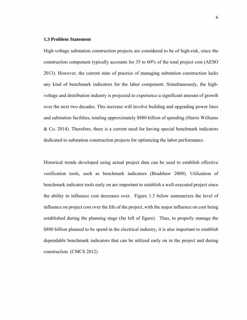
1.3 Problem Statement High-voltage substation construction projects are considered to be of high-risk, since the
construction component typically accounts for 35 to 60% of the total project cost (AESO
2013). However, the current state of practice of managing substation construction lacks
any kind of benchmark indicators for the labor component. Simultaneously, the high-
voltage and distribution industry is projected to experience a significant amount of growth
over the next two decades. This increase will involve building and upgrading power lines
and substation facilities, totaling approximately $880 billion of spending (Harris Williams
& Co. 2014). Therefore, there is a current need for having special benchmark indicators
dedicated to substation construction projects for optimizing the labor performance.
Historical trends developed using actual project data can be used to establish effective
verification tools, such as benchmark indicators (Bradshaw 2008). Utilization of
benchmark indicator tools early on are important to establish a well-executed project since
the ability to influence cost decreases over. Figure 1.3 below summarizes the level of
influence on project cost over the life of the project, with the major influence on cost being
established during the planning stage (far left of figure). Thus, to properly manage the
$880 billion planned to be spend in the electrical industry, it is also important to establish
dependable benchmark indicators that can be utilized early on in the project and during
construction. (CMCS 2012)

7
Figure 1.3 - Influence Curve for Construction Projects (CMCS 2012)
1.4 Research Objectives This study has two primary objectives. The first objective is to use comprehensive labor
hour data from actual electrical substation construction projects to establish typical labor
hour control points. These include using items defined further in Chapter 2 such as S-
curves, manpower loading curves, and other items like typical labor hour % per activity to
establish project labor control points. The second major objective is to identify other best
practices used to improve substation construction and overall project outcomes. These
include items such as typical project Work Breakdown Structure (WBS)5 and project
tracking tools.
1.5 Research Scope This study is focused on gathering qualitative labor hour data for completed high-voltage
substation projects only; high-voltage defined here as voltage levels greater than 69kV
5 Work Breakdown Structure (WBS) is a hierarchical breakdown of a project into manageable components. See Appendix B-Glossary for further definition and example.
8
including and up to 345kV, projects with voltages less than 69kV are not considered.
Labor, material, and equipment costs (in dollars) were not gathered for the research; this
was labor hour research only. The data collection and analysis process was also conducted
for “well-executed” projects only. A project was considered as “well-executed” if it was
identified to have the following characteristics:
0. Minimal to no change orders or requests for changes.
1. Minimal to zero safety recordable.
2. Minimal deviation in schedule duration.
3. Utilized contractor project management, tracking, and production reporting
throughout construction.
Actual data was provided from upper Midwest transmission owner for projects recently
completed by two different construction contractors. A total of 14 projects had labor data
collected for projects of various size and scope. The average size of the projects was
around 7,500 labor hours, with a range from about 1,000 - 22,000 labor hours. Substation
project types included step-down (change in voltage) and switching substations. The scope
of the substations included installing grass root substations (brand new facilities) and
addition or expansions to existing substation sites. The voltages of the substation projects
included in the study consisted of 345kV, 138kV, and 69kV. The configurations of the
substations also varied, including straight bus, ring bus, and breaker and a half
configurations.
9
As mentioned above, the scope of this study focused on above-grade activities for high-
voltage substation construction only, starting typically with setting of steel and ending on
above-grade scope substantial completion. Below ground activities were not included as
these typically are subcontracted out to various contractors, making labor hours difficult to
include and analyze consistently. The six (6) main above-grade substation activities that
were included within the research include:
1. Installing above-grade ground connections to equipment, steel structures, and
fencing.
2. Installing above-grade conduit, connections, and junction boxes.
3. Pulling and terminating of control cable and power cable (cable installation).
4. Setting steel supports for equipment, bus and switch supports, static masts,
dead-end H-frame or A-frame assemblies, etc. (steel installation).
5. Installing major equipment such as power transformers, circuit breakers,
disconnect switches, and all other minor above-grade equipment components.
6. Installing substation bus, bus connections, and hardware. This includes
installation of both rigid and strain bus, jumper connections to equipment,
insulators, and static shielding.
The majority of the collected projects utilized a design-assist delivery system in which the
owner, contractor, and engineering were engaged throughout the process. (Hart 2007) The
project contracts for projects involved were also primarily time and material (time and
equipment) contract type. The contractors considered in this study were also members of
major organizations such as the National Electrical Contractors Association (NECA),
Occupational Safety and Hazard Administration (OSHA), and the IBEW.

10
1.6 Research Methodology The process for gathering and analyzing the research data was completed in two stages.
The flowchart shown in Figure 1.4 below illustrates the two stages needed to facilitate the
research objectives outlined above. The first stage involved developing a survey, gathering
survey results, and inputting the data. The survey was initially put into word, and was then
transferred into an excel database for inputting the project data gathered. A template of the
survey that was put together is attached in Appendix C. This survey can be used as a
reference and template for future research within this line of study.
Stage 1: Data Collection and Inputs
Stage 2: Analysis and Benchmarks
Figure 1.4 - Process for Substation Benchmark Indicator Research
The most important information in the survey to gather was contractor actual data sheets,
such as actual labor hours for entire project by above-grade activity. This data was needed
to generate the outcomes listed within objective 1. Additional items requested in the survey
to be provided are highlighted below.
Project information, such as type, voltage, etc.;
Actual and planned contractor labor hours;
Actual and planned schedule durations;
Actual and planned peak manpower;
Actual and planned average manpower;
Develop Survey
Gather Survey Results
Input Data
Model Input Data
Check Model
Adequacy
Identify Benchmarking
& Control Indicators
11
Daily and/or weekly production and time reports
Timesheets for cost code breakout. (if available)
Scope summary documents or construction plans
The quantitative labor data collected from the contractor sheets for several projects was
also served as inputs into objective 2. Once the survey data and contractor input sheets
were gathered, the next step was to consolidate the data and establish a working database.
This involved inputting data such as project labor hours over the project lifecycle. This
was then used to derive the independent variables “Percent Complete of Project Duration”
and the dependent variables “Period of manpower as percentage of overall labor hours”.
For this research, a Microsoft Excel template sheet was established for inputting the data
into Microsoft Excel. An example of the template used for inputting the data can be found
in Appendix D.
The second stage of the research included developing model results, checking the adequacy
of the model thru the use of Minitab, and establishing typical benchmarks and control
indicators from the collected data. Model curves of the data were established with trend
lines, regression equations, and R2 values thru use of regression analysis. The regression
plots helped determine typical S-curve and manpower loading curves for substation above-
grade activities. Along with regression analysis, box-and-whisker plots were also
generated at this time to help define the average percent of labor hours per major substation
above-grade activity. The qualitative data was also inputted into excel for helping evaluate
the trends.

12
The next steps in stage 2 were to review the data analysis and report out on the findings.
Review of the data analysis involved initial checking the models generated for adequacy
and to review the model assumptions. This involved reviewing the R2 value closer, running
residual analysis within Minitab©, and summarizing the validation of the model. The final
step was to report out typical labor hour curves along with other trends and best practices
that were developed throughout the typical research findings.
1.7 Research Assumptions There were a few assumptions made during the collection and analysis of the data in the
research. The main assumptions that were used are bulleted below.
1. The weeks that had low labor hours reported during holidays (such as Christmas
and New Year’s, and or hunting season) were typically combined together.
2. For developing the manpower loading curve trends, the data was combined and
looked at on a monthly overall hours and durations.
3. Percent project time duration used on X-axis for the analysis is equivalent to
physical percent complete of project. Projects are assumed to have good production
as they were characterized as well-executed.
4. Design model analysis using linear regression analysis and the following model
assumptions.
a. Variables within the data is normally distributed.
b. Constant variance of the error predicted value, i.e. equal variance.
c. Samples are random, independent samples.

13
1.8 Summary With the electrical industry forecasted to rapidly grow, there is a need for research into
substation labor metrics to develop initial control indicators and to help practitioners
improve project performance. Having previous research conducted in other industries,
such as the mechanical and electrical building industries, sets the framework for outcomes
of the research and how the benchmark indicators developed can be used to improve the
overall project performance. Chapter 2 will further discuss literature review within the
industry, past benchmark indicators that have been developed, and how they have been
used. It will also briefly discuss the lack of labor trend research within the electrical
substation industry for labor trends and need for initial research.

14
CHAPTER TWO: LITERATURE REVIEW
2.1 Introduction Literature review was done within the construction industry to determine sectors that have
already begun to implement control indicators, typical benchmarking tools to utilize, and
how they can be used to improve project performance. Several electronic research tools
were utilized, including scholarly article search engines, past thesis documents, and other
searches such as via google.
The following section will provide examples of manpower loading curves and S-curves
found within other industries. The substation industry was also researched to identify the
need for project benchmarks and project control best practices, but no major labor hour
benchmark indicators were identified to be published in previous research.
2.2 Manpower Loading Curve: Definition, Use, and Trends in Other Industries Manpower loading curves provide a graphical representation on how the project labor
resources (in terms of labor hours or full time equivalent employees) are planned or
actually being expended throughout the time of the project (duration of the project in
percent of time or percent complete). (Hanna 2010) Having initial manpower curves at
the beginning of the project establishes a baseline plan for the project team to monitor and
evaluate as percent complete increases.

15
Figure 2.1 – Manpower Loading Curve Example for Planned Labor Hours (Chen 2006)
Figure 2.1 above shows a typical manpower loading curve, with the X-axis representing
the duration of the project (percent time) and the Y-axis representing the number of people
(or labor hours). (Chen 2006) The manpower curve above was developed using the
Trapezoidal Technique (TT). The TT is a simple, yet useful tool in helping show the
manpower buildup over the project, as well as show the typical cumulative resources that
are needed for the project. The cumulative resources that are needed are calculated by
taking the area under the trapezoidal curve. (Chen 2006) For planning purposes, this allows
the project team to initially forecast labor resources, see when the project will ramp up,
peak, and then run down, and provide justification for resource time and cost. (Clark 1985)
As stated earlier in the introduction, research into standardized manpower loading curves
provides specific control points, such as at what percent complete the project will peak and
what percent of labor hours are consumed at this point of the project. Standard manpower
curves, or calibration/benchmarking curves, can be put together by researching completed
projects that follow repeated work or patterns. (Clark 1985) Several other construction

16
industries, including the electrical building, HVAC contractors, and sheet metal contractors
have conducted research into manpower curves for their associated line of work. For
example, Awad S. Hanna and et. al conducted research of 59 projects within the Electrical
and Mechanical building contractors.
The trends of the manpower consumption for the electrical building projects researched
can be seen below in Figure 2.2. The figure shows the project duration on the X-axis in
terms of percentage of total time, and the Y-axis with the overall manpower as a percentage
of the peak manpower vs. the average manpower of the project. This shows that on
average, for the projects researched that at about 50-70% of the project duration is when
the peak to average ratio is greatest at around 160% calculated using the Allen trapezoidal
technique. (Hanna et al. 2002) This should be the primary timeframe of the project in
which the contractor (or owner) tracks, monitors, and reacts in better detail as it is the
critical time frame of the project. (Hanna et al. 2002)
Figure 2.2 - Electrical Building Contractor Manpower Loading Ex. (Hanna et al. 2002)

17
Similar to the research above, Hanna also has developed research into the HVAC and sheet
metal contractors using the trapezoidal technique. (Hanna et al. 2002) Hanna developed
specific control points along the project that indicated how many labor hours typically
should be consumed and at what durations for both types of projects. The data analysis
showed that on average, at about 50% of the project duration around 65% of the total labor
hours of the project should be consumed for sheet metal projects, and about 40% used at
50% of the time for mechanical projects. (Hanna et al 2002) Figures 2.3 and 2.4 below
show the trends that were developed for sheet metal and mechanical construction
respectively. These control points are important to help not only plan the project, but to
help the team gauge performance as the project takes place and react more proactively to
reduce cost and schedule overruns. (Hanna et al. 2002)
Figure 2.3 - Sheet Metal Contractor Manpower Loading Curve (Hanna et al. 2002)
Figure 2.4 - Mechanical Contractor Manpower Loading Curve (Hanna et al. 2002)

18
2.3 S-Curve: Definition, Use, and Trends in Other Industries
S-curves are similar to the manpower loading curves described above in that they are also
used to track planned labor over time. (Hanna et al. 2002) However, S-curves look at the
data on a cumulative scale to show how the labor progresses over time. (Chen 2006) When
plotted, the cumulative data over time typically resembles an “S” curve shape, hence the
typical “S-curve” name used in the industry. Figure 2.5 below shows an example of a
typical S-curve profile for a project with the different build-up, peak, and run-down stages.
The S-curve is developed by taking the area under the curve of the TT output, and then
plotting the cumulative labor hours on the Y-axis over time on the X-axis.
Figure 2.5 - S-Curve Example for Planned Cumulative Labor Hours (Chen 2006)
The planned S-curve can also then include actuals as the project progresses over time to
identify any variances in the planned labor hours. (Hanna et.al 2010) This provides

19
additional project controls for team members to evaluate from real time, and make
informed decisions based off especially if deviations occur. (Chen 2006) Figure 2.6 below
shows an example of this with the actual labor hours lagging over time when compared
against the plan. This could either mean that the project is behind schedule with low
production, or delayed. The project team members should use this data validation tool to
then properly analyze the project performance and take any corrective action as needed.
(Chen 2006)
Figure 2.6 - S-Curve with Actual vs. Planned Progress
(University of Wisconsin – Madison 2012)
Additional data, such as earned value technique could be used to determine project
performance, where earned value is the calculated by taking the base or estimated planned
hours multiplied by the percent complete. This can be done for the entire project, or by
main construction activities. (Hanna 2010) By adding the actual and earned value
components to the S-curve, the project management team can find ways to mitigate losses
before the project gets out of hand. (Hanna 2010)

20
Similar to the manpower loading curves produced above for sheet metal and electrical
building contractors, Hanna also produced a typical S-curve for sheet metal contractors
within the research. (Hanna 2010) Figure 2.7 below shows the typical cumulative labor
hours burned for sheet metal projects, with duration in time on the X-axis and cumulative
labor hours on the Y-axis. From the chart, it can be seen that at roughly 50% of the project
duration, the team should have expended only roughly 65% of the projects total labor
hours, which is consistent with the manpower loading trends shown earlier. This is a useful
visual tool to use for not only planning a project and cross checking of an estimate, but to
track actuals against for deviations as noted earlier.
Figure 2.7 - Typical S-Curve for Sheet Metal Contractors (Hanna et. al 2010)
Research into S-curve literature also showed that the transportation industry has developed
trends and control points as well. In 2012, the University of Wisconsin-Madison
Construction and Materials Support Center teamed up with WIS-DOT to research over 280
transportation construction projects. (CMCS 2012) From the research, the team was able
to develop a typical S-curve profile for cost instead of labor hours with a very high

21
statistical correlation (R2 value). The WIS-DOT research team also established a range of
control points based on the standard deviations of the averages calculated. (CMCS 2012)
Figure 2.8 below shows the S-curve and control points that were established from the WIS-
DOT research. The figure shows a fairly linear S-curve, with about 60% of the cost being
expended at around 60% of the project duration. This linear trend seems fairly accurate as
transportation road projects are fairly linear in nature with how they are constructed and
sequenced. (CMCS 2012)
Figure 2.8 - S-Curve and Control Points Transportation Projects (CMCS 2012)
2.4 Summary The literature review discussed above provides a framework for understanding manpower
loading curves and S-curves further, and how other industries are utilizing them. Even
though other industries have these benchmarks for high level trends, they still don’t provide
adequate correlations for substation construction sector, specifically since the activities and

22
equipment installations are different. Research was conducted on several major scholarly
article search engines, and labor hour control points could not be found for electrical
substation projects. Therefore, the research being conducted in this paper will provide a
missing component to the high-voltage industry and aid in establishing initial typical
control indicators for substation projects and establish a framework for future research in
this industry. The following chapter (Chapter 3) will discuss the characteristics of the
substation projects included within this research.
23
CHAPTER THREE: DATA CHARACTERISTICS
3.1 Introduction For this research, a total of 14 “well-executed” projects were gathered from an upper
Midwest transmission owner for projects completed by two different construction
contractors. As stated earlier, the focus of this research involved installation of substation
above-grade components only. The projects had various voltage types, scope (new,
expansion, size), and project labor hours. These projects were all conducted with the
contractor acting as the prime contractor for the above-grade scope of work being
researched. The sections below will further define the project types, voltage classes,
equipment types and equipment quantity ranges, along with project labor hour ranges.
3.2 Project Types, Locations, Use, and Voltages As mentioned above, 14 total “well-executed” electrical substation projects from the upper
Midwest were used within the research analysis. The 14 projects provided a sample from
two different substation contractors for substation projects with various type of substation
(new or expansion), overall functionality of the substation, location, and voltage class of
the project. The research included 8 new substations and 6 existing substations that were
being expanded. The majority of these projects involved installing a step-down substation6.
For example, 9 out of the 14 projects were characterized from the survey data as change in
voltage substations, while the remaining 5 were switching substations.
6 See Appendix B – Glossary for further definition of “step-down substation”. This is also commonly known as a “change in voltage” substation type.
24
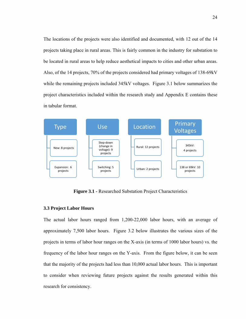
The locations of the projects were also identified and documented, with 12 out of the 14
projects taking place in rural areas. This is fairly common in the industry for substation to
be located in rural areas to help reduce aesthetical impacts to cities and other urban areas.
Also, of the 14 projects, 70% of the projects considered had primary voltages of 138-69kV
while the remaining projects included 345kV voltages. Figure 3.1 below summarizes the
project characteristics included within the research study and Appendix E contains these
in tabular format.
Figure 3.1 - Researched Substation Project Characteristics
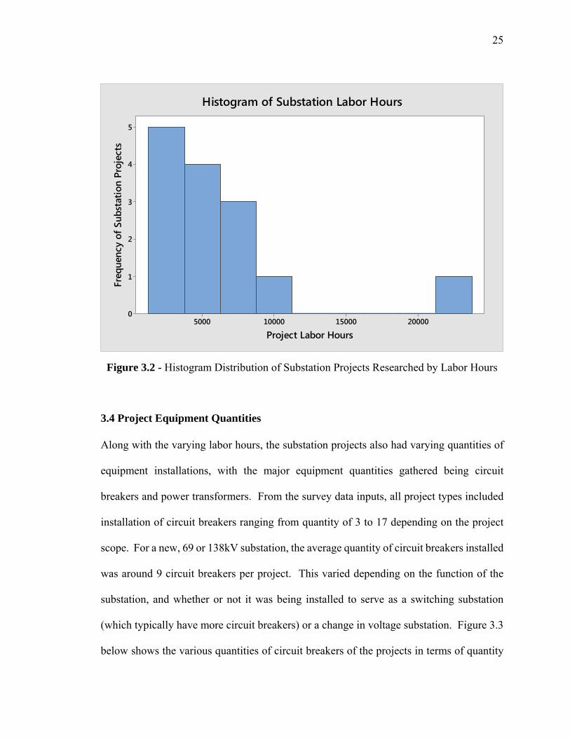
3.3 Project Labor Hours The actual labor hours ranged from 1,200-22,000 labor hours, with an average of
approximately 7,500 labor hours. Figure 3.2 below illustrates the various sizes of the
projects in terms of labor hour ranges on the X-axis (in terms of 1000 labor hours) vs. the
frequency of the labor hour ranges on the Y-axis. From the figure below, it can be seen
that the majority of the projects had less than 10,000 actual labor hours. This is important
to consider when reviewing future projects against the results generated within this
research for consistency.
Type
New: 8 projects
Expansion: 6 projects
Use
Step‐down (change in voltage): 9 projects
Switching: 5 projects
Location
Rural: 12 projects
Urban: 2 projects
Primary Voltages
345kV:
4 projects
138 or 69kV: 10 projects
25
Figure 3.2 - Histogram Distribution of Substation Projects Researched by Labor Hours
3.4 Project Equipment Quantities Along with the varying labor hours, the substation projects also had varying quantities of
equipment installations, with the major equipment quantities gathered being circuit
breakers and power transformers. From the survey data inputs, all project types included
installation of circuit breakers ranging from quantity of 3 to 17 depending on the project
scope. For a new, 69 or 138kV substation, the average quantity of circuit breakers installed
was around 9 circuit breakers per project. This varied depending on the function of the
substation, and whether or not it was being installed to serve as a switching substation
(which typically have more circuit breakers) or a change in voltage substation. Figure 3.3
below shows the various quantities of circuit breakers of the projects in terms of quantity
2000015000100005000
5
4
3
2
1
0
Project Labor Hours
Freq
uenc
y of
Sub
stat
ion
Proj
ects
Histogram of Substation Labor Hours

26
of circuit breakers on the X-axis (Each) vs. the frequency of the number of projects that
had that range of circuit breakers on the Y-axis. From this, it can be seen that the majority
of the substation projects had 4-10 circuit breakers.
Figure 3.3 - Histogram Distribution of Substation Projects Included by Circuit Breaker
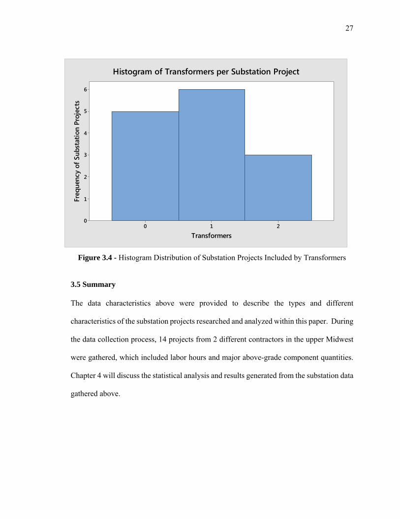
The number of voltage transformers were also requested within the survey and documented
for research analysis. The range of number of transformers on the projects ranged from 0
(primarily for switching substations) to 2 (primarily for new 345 and 138 kV substations).
Figure 3.4 below shows the distribution of transformer ranges from 0, 1, to 2 on the X-axis
and frequency of the transformer quantity ranges on the Y-axis. From this, it can be seen
that the sample size was fairly uniformly distributed (bell-shaped).
161284
4
3
2
1
0
Circuit Breakers
Freq
uenc
y of
Sub
stat
ion
Proj
ects
Histogram of Circuit Breakers per Substation Project
27
Figure 3.4 - Histogram Distribution of Substation Projects Included by Transformers
3.5 Summary The data characteristics above were provided to describe the types and different
characteristics of the substation projects researched and analyzed within this paper. During
the data collection process, 14 projects from 2 different contractors in the upper Midwest
were gathered, which included labor hours and major above-grade component quantities.
Chapter 4 will discuss the statistical analysis and results generated from the substation data
gathered above.
210
6
5
4
3
2
1
0
Transformers
Freq
uenc
y of
Sub
stat
ion
Proj
ects
Histogram of Transformers per Substation Project

28
CHAPTER FOUR: DATA ANAYLSIS - CONTROL INDICATOR RESULTS
4.1 Introduction After documenting the project characteristics in Chapter 3, the next step of the research
was to develop typical benchmark indicators for substation labor as set out in the
objectives. Tools such as manpower loading curves, S-curves, and boxplots were used to
identify typical benchmark indicators. The primary method for analyzing the data involved
plotting the actual labor hours and then running a regression analysis (as noted earlier in
the assumptions section) for the data points.
To recap what was discussed earlier in Chapter 1 under the “Research Methodology”
section, a regression analysis was used to plot a typical regression curve (or model) for the
manpower over time and also to derive prediction equations for standard substation curves.
These results were then used to show how well the predicted equation can be used to
generate a response variable. For our models, the response variable (Y-axis) is “percent
cumulative labor hours” for the S-curve and “percent of above-grade hours/average hours”
for the manpower loading curves. The response variables mentioned above are dependent
on the independent variable (X-axis), which for this research is “percent time” defined as
the duration of time for completing the above-grade scope of work.
Along with the regression analysis, additional statistical analysis was ran in Minitab© to
determine S-value, P-values, F-values, and to also check the adequacy of the regression
model using residual analysis plots. Boxplots (also known as box-and-whisker plots) were
29
completed for the average percent of labor hours by task, which will further be defined as
the activity contribution factor (ACF), and schedule durations. This was done to provide
a range of typical values versus reporting out a single average. The benchmark indicator
results were developed either through the use of Microsoft Excel (primarily for Regression
analysis) or Minitab© statistical software (for additional statistical analysis values,
checking model adequacy, and box plots).
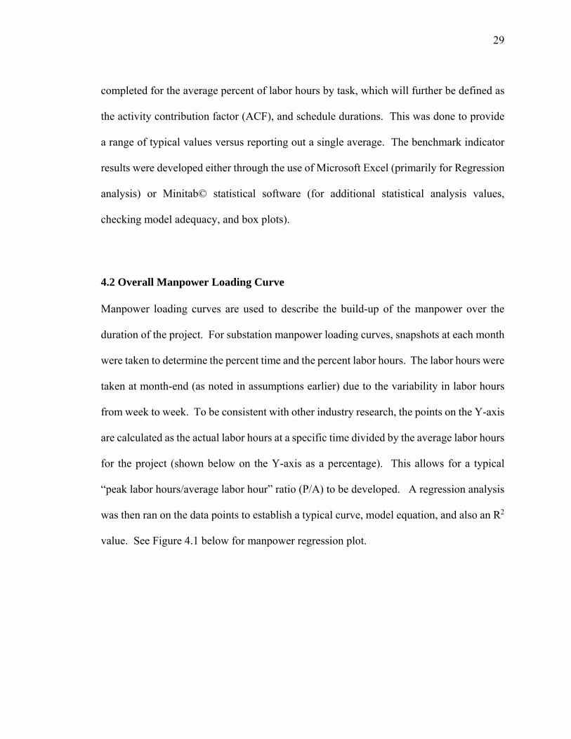
4.2 Overall Manpower Loading Curve Manpower loading curves are used to describe the build-up of the manpower over the
duration of the project. For substation manpower loading curves, snapshots at each month
were taken to determine the percent time and the percent labor hours. The labor hours were
taken at month-end (as noted in assumptions earlier) due to the variability in labor hours
from week to week. To be consistent with other industry research, the points on the Y-axis
are calculated as the actual labor hours at a specific time divided by the average labor hours
for the project (shown below on the Y-axis as a percentage). This allows for a typical
“peak labor hours/average labor hour” ratio (P/A) to be developed. A regression analysis
was then ran on the data points to establish a typical curve, model equation, and also an R2
value. See Figure 4.1 below for manpower regression plot.

30
Figure 4.1 - Manpower Loading Curve for Overall Above-grade Construction
Figure 4.1 above shows the individual points that were plotted (blue dots) for the project
along with the regression analysis trend line (solid blue line). From the regression analysis,
the bell shaped trend shows that the labor hours typically peak around 50% with a ~180%
peak to average ratio. The R2 value, which is shown under the equation in Figure 4.1 for a
fourth order polynomial, was calculated as R2 = 0.7605. The higher the R2 value, the better
the model generally fits with the data set. The 0.7605 value that was calculated is consistent
with similar mechanical manpower loading curves published in the mechanical and
electrical building industry. (Hanna et al. 2002) This will be checked initially in section
4.3 with residual analysis.

31
Figure 4.2 - Minitab© Regression Analysis for Overall Above-grade Construction
In addition to the Microsoft Excel analysis shown above in figure 4.1, the data points were
plotted within Minitab© to confirm the manpower loading curve research findings and
regression analysis. As shown in Figure 4.2, the results of the cubic regression analysis in
Minitab© are consistent to the Excel fourth order analysis with a R2 value of 0.728. Again,
this R2 value falls in line with other research. Along with model fit, dotted lines are also
included to represent prediction intervals (PIs). The PI lines are provide a range of values
for outputs (+/-) 5% from the typical value of interest. The results from Minitab© also
include the calculated S-value which indicates the standard error of the estimate. For model
fits, a smaller S-value is desired as it further indicates that the data points fit close to the
fitted line. (Frost 2014) As seen above in the right hand side of Figure 4.2, the S-value for
the cumulative substation manpower curve was calculated as S=0.42. From the analysis,
1.00.80.60.40.20.0
300.00%
200.00%
100.00%
0.00%
-100.00%
S 0.420094R-Sq 72.8%
x
y
Regression95% CI95% PI
Manpower Loading Plots for Substation Above-Grade y = - 0.1003 + 7.897 x
- 9.671 x^2 + 1.774 x^3
32
we conclude that the model appears to be adequate for a typical, high level trend.
Additional data collection and statistical analysis could be done in future research to help
improve the R2 and statistical values shown above.
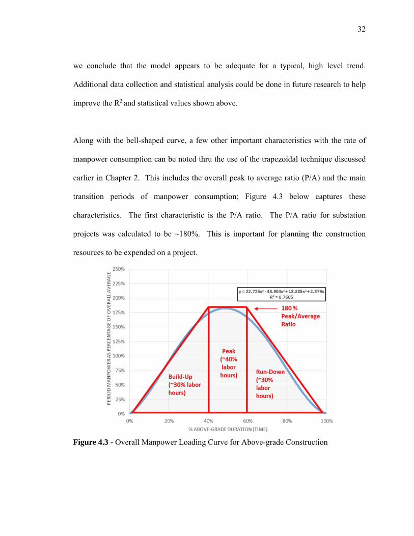
Along with the bell-shaped curve, a few other important characteristics with the rate of
manpower consumption can be noted thru the use of the trapezoidal technique discussed
earlier in Chapter 2. This includes the overall peak to average ratio (P/A) and the main
transition periods of manpower consumption; Figure 4.3 below captures these
characteristics. The first characteristic is the P/A ratio. The P/A ratio for substation
projects was calculated to be ~180%. This is important for planning the construction
resources to be expended on a project.
Figure 4.3 - Overall Manpower Loading Curve for Above-grade Construction

33
The second characteristic is that the trapezoidal technique divides the manpower loading
curve into three main stages: build-up, peak, and run-down. The build-up of manpower
occurs between 0% – 40% of the project duration, accounting for approximately 30% of
the project labor hours. The peak stage occurs between 40 – 60% of the project duration,
accounting for approximately 40% of the project labor hours. This is consistent with the
industry research results presented earlier in Chapter 2 in which mechanical and electrical
building researched showed 40% labor hours during peak time. During the peak stage, the
project team should carefully plan, track, and monitor the labor component of the project
because the bulk of labor hours is expended over a short timeframe (Hanna et al. 2002).
Lastly, the run-down stage typically occurs between 60% – 100% of the project duration,
accounting for the remaining 30% of the project labor hours.
4.3 Minitab© Residual Analysis for Overall Manpower Loading Curves After plotting the manpower loading curves in excel and Minitab©, further analysis was
conducted in Minitab© to run initial checks on the model curve for adequacy and to check
the assumptions made earlier. This involved performing a residual analysis with plots to
analyze the residuals. A residual represents how much the actual response deviates from
the fitted model. (Kouiden 2012) For the analysis, a smaller residual is desired as this
indicates a well fit model. Figure 4.4 below shows the residual plot analysis for the
manpower loading curve presented in section 4.2. See Appendix F1 for more Minitab©
report results.
34
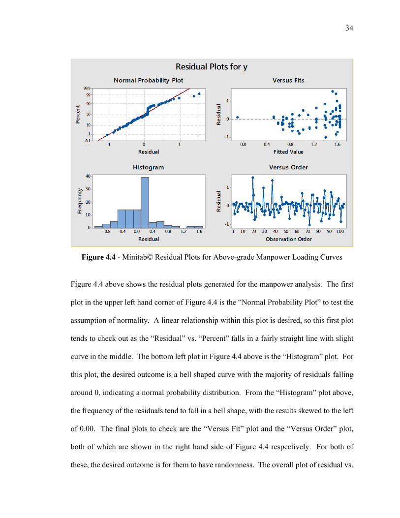
Figure 4.4 - Minitab© Residual Plots for Above-grade Manpower Loading Curves
Figure 4.4 above shows the residual plots generated for the manpower analysis. The first
plot in the upper left hand corner of Figure 4.4 is the “Normal Probability Plot” to test the
assumption of normality. A linear relationship within this plot is desired, so this first plot
tends to check out as the “Residual” vs. “Percent” falls in a fairly straight line with slight
curve in the middle. The bottom left plot in Figure 4.4 above is the “Histogram” plot. For
this plot, the desired outcome is a bell shaped curve with the majority of residuals falling
around 0, indicating a normal probability distribution. From the “Histogram” plot above,
the frequency of the residuals tend to fall in a bell shape, with the results skewed to the left
of 0.00. The final plots to check are the “Versus Fit” plot and the “Versus Order” plot,
both of which are shown in the right hand side of Figure 4.4 respectively. For both of
these, the desired outcome is for them to have randomness. The overall plot of residual vs.

35
fits is used to check the assumption of constant variance. From the analysis, the fitted plot
does tend to be random, but also does sort of have an increasing in residuals to the right.
This could suggest that further analysis and statistical plots be conducted to improve the
model and check the assumption of constant variance. The residual vs. order is used to
check the assumption of independent samples. This plot changes signs rapidly (but not one
right after the other), but also does have random fluctuation pattern around the centerline
which help indicate randomness. Further statistical analysis, transformations, and data
collection should be done with future research to help confirm the initial model findings
provided above with the regression analysis and to verify the assumptions made initially.
4.4 Manpower Loading Curves by Above-grade Activity Along with the manpower loading curve for the entire substation project, the research also
looked into manpower loading curves for individual above-grade activities. The resulted
individual manpower curves, shown in Figure 4.5, highlight three main findings: activity
manpower features, project milestones, and activity progression principles.
Figure 4.5 - Individual Manpower Loading Curves by Above-grade Activity

36
Activity Manpower Features
The building up of individual activities along with their P/A ratios are illustrated in Figure
4.5. Data analysis shows that steel, conduit, and cable installations have fairly steep
manpower build-ups. Accordingly, practitioners should anticipate a high build-up rate for
steel installation during the first 15% of project duration. Likewise, a high build-up rate for
the conduit installation should be foreseen roughly in the time period between 15% and
30% of project duration. Similarly, a high build-up rate for cable installation should
typically be expected in the time period between 20% and 40%. Moreover, Figure 4.5
reveals that steel installation usually has the highest P/A ratio (235%) at 20% of project
duration, followed by conduit installation (230%) at 40% of project duration. On the other
hand, grounding typically has the lowest P/A ratio (150%) achieved at 50% of project
duration. This aligns with the fact that grounding completion does not typically impact the
start of other activities.
Project Milestones
Based on data analysis, this paper deduces that all major project activities should start in
the first 30% of project duration. This benchmark indicator should be used by practitioners
as an early warning sign of poor project performance in order to mitigate negative impacts.
Moreover, data analysis shows that steel installation, major equipment installation, and
grounding typically start in the time period between 0% and 5% of the project duration.
The time period between 10% and 25% of project duration typically experiences the start
of the remaining three activities: conduit installation, cable installation, and bus work.

37
Activity Progression Principles
From a scheduling perspective, this paper provides sequencing principles for above-grade
substation construction activities. Figure 4.6 shows a simplified linear sequencing pattern
for the start of activities. Normally, steel and major equipment installations should start
early in the project timeframe since remaining activities are dependent on them. Similarly,
conduit installation needs to start prior to cable installation. However, these findings do not
dictate a finish-to-start relationship between activities. Instead, reasonable overlapping
normally takes place as shown in Figure 4.5.
Figure 4.6 - Simplified Linear Sequence of the Start of Above-grade Activities
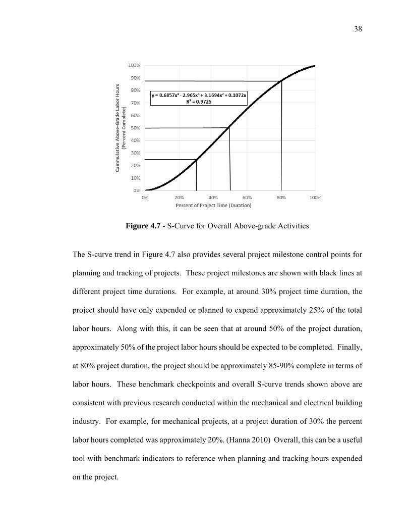
4.5 Overall Project S-Curve Along with the manpower loading curves, typical S-curves are another means for
illustrating how labor hours can be planned or expended over time and to develop
benchmark indicators. For the substation research, this was done by plotting cumulative
labor hours for the 14 projects over time in Microsoft Excel, and then running a regression
analysis for the plotted points. Figure 4.7 below shows the analysis that was conducted,
with the regression trend line plotted as a solid blue line. From this, it can be seen that the
trend line fits well with the data points with a high R2 value of 0.972.
Steel (Red)
Major Equipment (Orange)
Grounding (Blue)
Conduit Installation (Black)
Cable Installation (Green)
Bus Installation (Purple)
38
Figure 4.7 - S-Curve for Overall Above-grade Activities
The S-curve trend in Figure 4.7 also provides several project milestone control points for
planning and tracking of projects. These project milestones are shown with black lines at
different project time durations. For example, at around 30% project time duration, the
project should have only expended or planned to expend approximately 25% of the total
labor hours. Along with this, it can be seen that at around 50% of the project duration,
approximately 50% of the project labor hours should be expected to be completed. Finally,
at 80% project duration, the project should be approximately 85-90% complete in terms of
labor hours. These benchmark checkpoints and overall S-curve trends shown above are
consistent with previous research conducted within the mechanical and electrical building
industry. For example, for mechanical projects, at a project duration of 30% the percent
labor hours completed was approximately 20%. (Hanna 2010) Overall, this can be a useful
tool with benchmark indicators to reference when planning and tracking hours expended
on the project.
39
Along with the milestone checkpoints, the S-curve can also be plotted with typical upper
and lower bounds across the duration of the project. The control points for this research
were done in Excel by using a similar process previously established in the WDOT
research. (CMCS 2012) This involved taking blocks of time ranges, calculating the average
percent of time, and the average percent of hours for those specific time ranges. The block
of time ranges were then plotted along the X-axis. The control points were then calculated
by adding and subtracting the standard deviation to the average labor hours. The control
points were then plotted along the Y-axis and combined within the chart shown earlier in
Figure 4.7.
The data for this procedure can be seen below in Table 4.1 with the plot of the data then
shown below that in Figure 4.8. From these control points, a range approach can be used
to further identify deviations in the labor hours. For example, if a project is being
monitored at time duration of 30% (X-axis) and is determined to have expended 40% of
the labor hours, this should be a red-flag to the project team to review as it is already outside
the typical upper bound for labor hours. This allows for earlier detection of deviations and
potential mitigation of future labor overruns. These ranges can also be adjusted for different
deviations depending on the risk of the project.
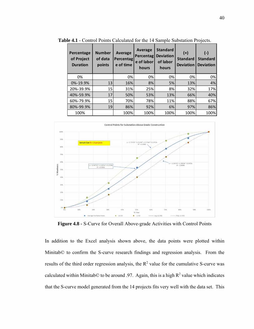
40
Table 4.1 - Control Points Calculated for the 14 Sample Substation Projects.
Figure 4.8 - S-Curve for Overall Above-grade Activities with Control Points
In addition to the Excel analysis shown above, the data points were plotted within
Minitab© to confirm the S-curve research findings and regression analysis. From the
results of the third order regression analysis, the R2 value for the cumulative S-curve was
calculated within Minitab© to be around .97. Again, this is a high R2 value which indicates
that the S-curve model generated from the 14 projects fits very well with the data set. This
Percentage
of Project
Duration
Number
of data
points
Average
Percentag
e of time
Average
Percentag
e of labor
hours
Standard
Deviation
of labor
hours
(+)
Standard
Deviation
(‐)
Standard
Deviation
0% 0% 0% 0% 0% 0%
0%‐19.9% 13 16% 8% 5% 13% 4%
20%‐39.9% 15 31% 25% 8% 32% 17%
40%‐59.9% 17 50% 53% 13% 66% 40%
60%‐79.9% 15 70% 78% 11% 88% 67%
80%‐99.9% 19 86% 92% 6% 97% 86%
100% 100% 100% 100% 100% 100%
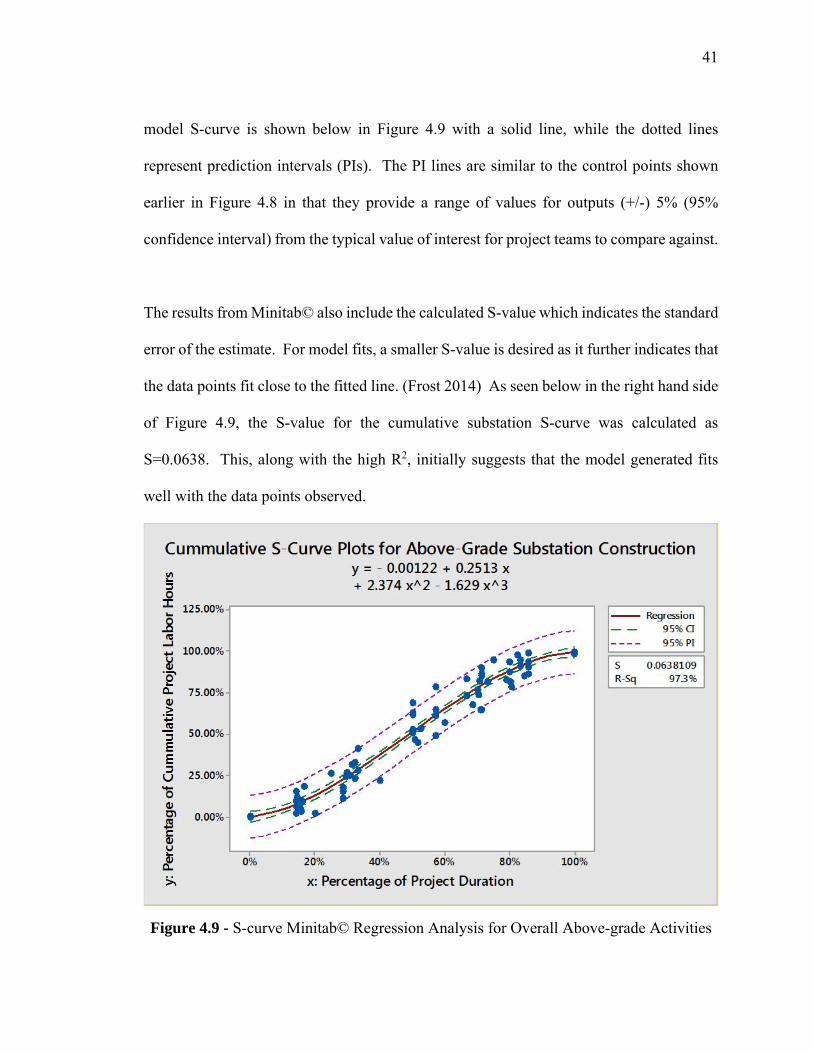
41
model S-curve is shown below in Figure 4.9 with a solid line, while the dotted lines
represent prediction intervals (PIs). The PI lines are similar to the control points shown
earlier in Figure 4.8 in that they provide a range of values for outputs (+/-) 5% (95%
confidence interval) from the typical value of interest for project teams to compare against.
The results from Minitab© also include the calculated S-value which indicates the standard
error of the estimate. For model fits, a smaller S-value is desired as it further indicates that
the data points fit close to the fitted line. (Frost 2014) As seen below in the right hand side
of Figure 4.9, the S-value for the cumulative substation S-curve was calculated as
S=0.0638. This, along with the high R2, initially suggests that the model generated fits
well with the data points observed.
Figure 4.9 - S-curve Minitab© Regression Analysis for Overall Above-grade Activities

42
Along with the S-curve Minitab© plot, Minitab© reports were also ran to calculate the
statistical P and F-values which can be further used to check the results generated from the
data set. From Minitab©, the P-value and F-Values for the cumulative S-curve cubic model
were calculated as 0.000 and 43.14 respectively. For this research, our null hypothesis (Ho)
(devil’s advocate) would be that the model fitted has no correlation (no predictive
capability) with the data collected. Our alternative hypothesis (Ha) would then be that there
is a correlation within the data collected. If the P-value is low, we reject our null
hypothesis and state that our model fit does provide a correlation to the data set. With the
P-value from the analysis at 0.000, we initially conclude that our model fits well with the
data set, reject our null hypotheses and accept our alternative hypothesis.
Similarly, a large F-value indicates that we would reject our null hypothesis. With an F-
value from the analysis of 43.14, we reject our null hypothesis again and conclude that the
model again has initial predictive capability. So with both the P and F values checking out,
we conclude that our model once again tends to fit well with the data set for the substation
cumulative S curves. Please see Appendix F2 for additional Minitab© report summary
with the P and F-values.
4.6 Minitab© Residual Analysis for Substation Above-grade Scope S-curves Similar to the residual plots discussed in Section 5.2.2, this was also done for the S-curve
results above to initially check the model for adequacy and to check the assumptions made
earlier. Figure 4.10 below shows the residual plots generated for the S-curve analysis. The

43
first plot in the upper left hand corner of Figure 4.10 is the “Normal Probability Plot”. A
linear relationship within this plot is desired, so this first plot appears to check out as the
“Residual” vs. “Percent” tends to fall in a fairly straight line. The bottom left plot in Figure
4.10 above is the “Histogram” plot. For this plot, the desired outcome is a bell shaped
curve with the majority of residuals falling around 0, indicating a normal probability
distribution. From the “Histogram” plot, the frequency of the residuals primarily fall along
0.00 with a bell shaped pattern, so this tends to check out as well. The final plots to check
are the “Versus Fit” plot and the “Versus Order” plot, both of which are shown in the right
hand side of Figure 4.10 respectively. For both of these, the desired outcome is for them
to have randomness. The overall plot of residual vs. order appears to be random around
the centerline and doesn’t seem to have any glaring patterns. The fitted value vs. residual
also appears to be constant with a somewhat of a horizontal pattern, and minimal fanning.
This helps support and initially indicates the assumption of constant variances to be true.
Additional data collection, statistical analysis, and model checks should be done to further
test the initial model results presented above and assumptions provided in this research.
Figure 4.10 - Minitab© Residual Plot for Overall Above-grade S-Curve
0.20.10.0-0.1-0.2
99.999
90
50
10
1
0.1
Residual
Perc
ent
1.000.750.500.250.00
0.2
0.1
0.0
-0.1
-0.2
Fitted Value
Residu
al
0.150.100.050.00-0.05-0.10-0.15
40
30
20
10
0
Residual
Freq
uenc
y
9080706050403020101
0.2
0.1
0.0
-0.1
-0.2
Observation Order
Residu
al
Normal Probability Plot Versus Fits
Histogram Versus Order
Residual Plots for y
44
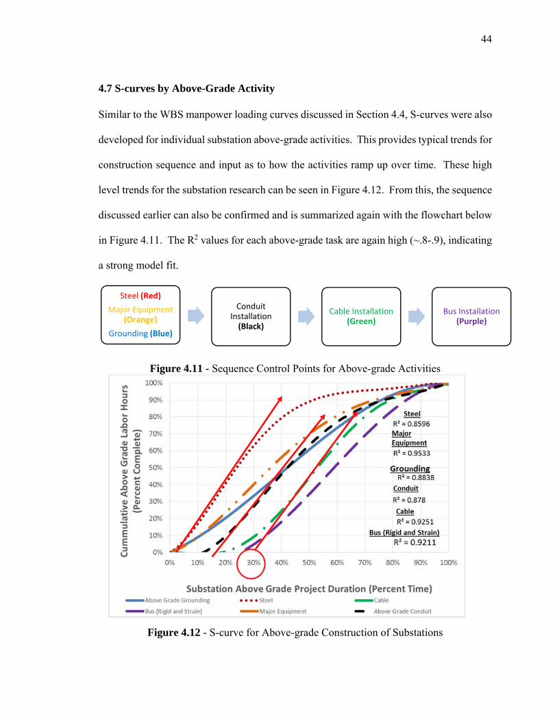
4.7 S-curves by Above-Grade Activity Similar to the WBS manpower loading curves discussed in Section 4.4, S-curves were also
developed for individual substation above-grade activities. This provides typical trends for
construction sequence and input as to how the activities ramp up over time. These high
level trends for the substation research can be seen in Figure 4.12. From this, the sequence
discussed earlier can also be confirmed and is summarized again with the flowchart below
in Figure 4.11. The R2 values for each above-grade task are again high (~.8-.9), indicating
a strong model fit.
Figure 4.11 - Sequence Control Points for Above-grade Activities
Figure 4.12 - S-curve for Above-grade Construction of Substations
Steel (Red)
Major Equipment (Orange)
Grounding (Blue)
Conduit Installation (Black)
Cable Installation (Green)
Bus Installation (Purple)
45
From Figure 4.12 above, it can again be seen that steel, conduit, and cable installations
typically have a fairly steep ramp of cumulative manpower with both of these having a
fairly steep-linear line. Also, the figure above again demonstrates that at 30% project
duration, all above-grade activities should typically be started and/or in progress. Once the
project is around 50% time duration, steel and conduit should primarily be done, and the
cable and bus installations should be about 45% and 35% completed respectively. These
project duration points can again be used as a high-level milestone check for planning and
tracking of a project. For example, during the planning of a project if all activities are
shown to start around 15% time duration, the project team could question if the schedule
is too aggressive and discuss why that might be. It also can be used for tracking of a project
to check for production issues as labor hours are actualized. For example, if a typical
substation project is ongoing and reporting at 50% time duration that the steel is only at
30% labor hours complete, this should initiate a warning sign to the project team for them
to stop and review the projects production performance as it might be critically falling
behind a typical schedule.
4.8 Activity Contribution Factors (ACFs) The results above provide a good means for checking how the labor is planned and tracked
over the duration of the project with typical control point indicators. One other method to
check the overall project during the planning stage for estimate accuracy is to determine
the activity contribution factor (ACF). For this paper, ACF is defined as the typical labor
hour percentages per construction activity. The ACF can be used not only for determining
high level estimates, but to also run a quick check of an estimate.

46
For this research, this was initially done within Excel by taking a ratio of the above-grade
activity labor hours divided by the total above-grade labor hours of the project. The
calculated percentages for each project were then averaged together and plotted in the pie
chart below in Figure 4.13. From this, it can be seen that the installation of major
equipment (~23%), bus installation (~25%), and cable installations make (~24%) up ~75%
of the project labor hours. With only 25% of the other areas compiling the rest of the labor
hours, a typical 80-20 percent rule should generally be used for planning and monitoring
of tasks.
Figure 4.13 - Typical Percentage of Labor Hours per Above-grade Activities
Along with the pie chart above, which contains information based on all types of substation
projects, a table was set up to see if the type of project has significant impact on the
averages per task. Table 4.2 below summarized these findings. From the results presented
below, the type of project doesn’t seem to significantly impact the averages lists as the
major above-grade activities, such as cable installations, major equipment, and bus
% Above Grade Grounding
10%% Above Grade Conduit and Junction Box
6%
% Control/Power Cable (Pull and Termination)
24%
% Setting Support Steel
12%
% Installing Major
Equipment 23%
% Bus (strain, rigid, connectors)
25%

47
installation still comprise the majority percentage of the labor hours. From this, it can be
seen that for the majority of the projects, around 75% of the labor hours should fall within
these activities. These items are boxed in red below in Table 4.2.
Table 4.2 – Percentage of Labor Hours per Above-grade Activities
One additional statistical analysis that can be done for ACFs is to develop a box-and-
whisker plot analysis, also known as a boxplot. A box-and-whisker plot is used as a visual
plot to understand the distribution of the averages and to show the median. This plot also
shows variability of the averages, typical tendencies of the data set, outliers, and upper and
lower quartiles. (Minitab 2014) This can be beneficial to project teams as it provides more
of a range of values approach for them to review against instead of a straight, single point
average. For this substation research, the data calculated within Excel was taken and
copied into the Minitab© statistical software package. Using Minitab’s© boxplot
generating tool, the following results shown in Figure 4.14 were generated.
Calculation% Above
Grade Grounding
% Above Grade
Conduit and Junction Box
% Control/Pow
er Cable (Pull and
% Setting Support
Steel
% Installing Major
Equipment
% Bus (strain, rigid, connectors)
Average New (Greenfield) N = 8 10% 7% 23% 11% 23% 26%
Average Addition or Expansion N = 6 8% 5% 24% 15% 23% 25%
Average Change in Voltage N = 9 8% 6% 24% 12% 24% 26%
Average Substation Switching N = 5 12% 5% 24% 13% 21% 24%

48
Figure 4.14 - Activity Contribution Factors (ACFs) of the Above-grade Activities
From the Minitab© boxplot above, the results infer that bus (~25%), cable (~25%), and
major equipment (~23%) installations have the highest ACFs, collectively comprising
approximately 75% of above-grade project labor hours. Therefore, it is recommended that
practitioners should utilize more time for planning and tracking these activities. Moreover,
the upper and lower quartiles of the box-and-whisker plots show that these activities have
high variability with regard to their ACF. This variability can be attributed to the fact that
these activities are typically impacted by different substation types, voltage classes, and
design configurations.
Bus Ins
ta llatio
n
Major E
quipmen
t
Steel Ins
tallatio
n
Cable In
stalla
tion
Above-G
rade C
onduit
Above-G
rade G
rounding
35.00%
30.00%
25.00%
20.00%
15.00%
10.00%
5.00%
0.00%
Perc
ent L
abor
Hou
rs p
er C
onst
ruct
ion
Activ
ity
Activity Contribution Factor for Above-Grade Substation Activities
*75% of project labor hours circled in red.
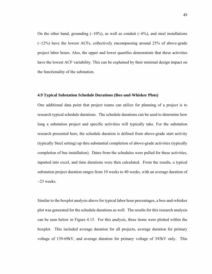
49
On the other hand, grounding (~10%), as well as conduit (~6%), and steel installations
(~12%) have the lowest ACFs, collectively encompassing around 25% of above-grade
project labor hours. Also, the upper and lower quartiles demonstrate that these activities
have the lowest ACF variability. This can be explained by their minimal design impact on
the functionality of the substation.
4.9 Typical Substation Schedule Durations (Box-and-Whisker Plots) One additional data point that project teams can utilize for planning of a project is to
research typical schedule durations. The schedule durations can be used to determine how
long a substation project and specific activities will typically take. For the substation
research presented here, the schedule duration is defined from above-grade start activity
(typically Steel setting) up thru substantial completion of above-grade activities (typically
completion of bus installation). Dates from the schedules were pulled for these activities,
inputted into excel, and time durations were then calculated. From the results, a typical
substation project duration ranges from 10 weeks to 40 weeks, with an average duration of
~23 weeks.
Similar to the boxplot analysis above for typical labor hour percentages, a box-and-whisker
plot was generated for the schedule durations as well. The results for this research analysis
can be seen below in Figure 4.15. For this analysis, three items were plotted within the
boxplot. This included average duration for all projects, average duration for primary
voltage of 139-69kV, and average duration for primary voltage of 345kV only. This
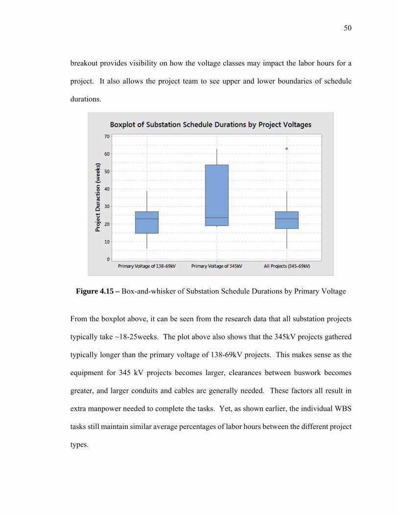
50
breakout provides visibility on how the voltage classes may impact the labor hours for a
project. It also allows the project team to see upper and lower boundaries of schedule
durations.
Figure 4.15 – Box-and-whisker of Substation Schedule Durations by Primary Voltage
From the boxplot above, it can be seen from the research data that all substation projects
typically take ~18-25weeks. The plot above also shows that the 345kV projects gathered
typically longer than the primary voltage of 138-69kV projects. This makes sense as the
equipment for 345 kV projects becomes larger, clearances between buswork becomes
greater, and larger conduits and cables are generally needed. These factors all result in
extra manpower needed to complete the tasks. Yet, as shown earlier, the individual WBS
tasks still maintain similar average percentages of labor hours between the different project
types.
51
Also, the boxplots above provide upper and lower quartiles for the different project
voltages to check against. For example, for the 138-69kV primary voltage projects, it could
be more common to see projects with a range of 15-25 weeks. If a project is initially
scheduled for primary voltages of 138-69kV to only take 10 weeks, this schedule might be
too compressed and needing longer workdays to complete within the time period. A
compressed schedule, which can involve working 6-10 hour days or 7-10 hour days,
typically results in loss of production and inefficiencies. (Whiteside 2006) The project
team should question this schedule as it tends to be aggressive when compared against
these typical results, and determine if it changes are needed and adjust accordingly.
4.10 Summary Chapter 4 discussed the major findings of the substation above-grade scope research. The
regression analysis ran within the labor hour data over time produced manpower loading
curves and S-curves that allowed typical benchmark indicators and control points to be
identified. Results for typical percentages of labor hours per above-grade activity and
schedule durations were also developed with boxplots used to further display the results.
Chapter 5 will highlight best practices that were identified to be used for the projects
research.
52
CHAPTER FIVE: BEST PRACTICES
5.1 Introduction
Along with developing standard manpower loading curves and S-curves, the research
identified other typical Best Practices to complete objective 2 of the research. Best
Practices include tools that the project teams utilized to help aid in establishing project
success, such as reporting and tracking mechanisms, and establishing a Work Breakdown
Structure (WBS). The following sections will discuss additional Best Practices that were
identified and how they could potentially be used to improve substation project outcomes.
5.2 Work Breakdown Structure (WBS) and Substation WBS Example Work Breakdown Structure (WBS) can be used to break down a project into manageable
work components. This allows for better overall scope management and provides a visual
structure of the work to be completed. Once a WBS is set up and understood by the team
members, it can then be used to establish accountability, plan the project, and provide a
framework for managing cost and schedule control.
For the substation projects researched, establishing a WBS was identified as a useful tool
for either the electrical owner or contractor to put together. Based on the research and data
collected, a sample WBS structure was put together for the above-grade scope for a typical
new substation project. Figure 5.1 below provides a typical substation WBS example. The
example provided bellow lists the above-grade activities that need to be completed. With
substation WBS tasks of cable pulling, bus installation, and major equipment making up
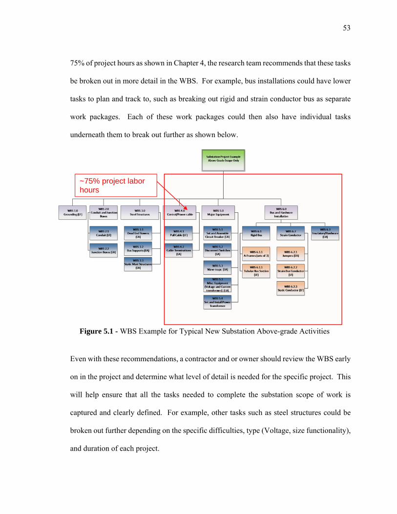
53
75% of project hours as shown in Chapter 4, the research team recommends that these tasks
be broken out in more detail in the WBS. For example, bus installations could have lower
tasks to plan and track to, such as breaking out rigid and strain conductor bus as separate
work packages. Each of these work packages could then also have individual tasks
underneath them to break out further as shown below.
Figure 5.1 - WBS Example for Typical New Substation Above-grade Activities
Even with these recommendations, a contractor and or owner should review the WBS early
on in the project and determine what level of detail is needed for the specific project. This
will help ensure that all the tasks needed to complete the substation scope of work is
captured and clearly defined. For example, other tasks such as steel structures could be
broken out further depending on the specific difficulties, type (Voltage, size functionality),
and duration of each project.
~75% project labor hours

54
5.3 Field Tracking and Timesheet Reporting Once the WBS is set up early on in a project, the contractor should begin to determine how
to then plan the project, track, and report out on the construction progress. The WBS can
be used as an input to determine the level of detail to track to, and what specific items
should be tracked and monitored closer.
From the research, several best practices in terms of tracking and monitoring were
identified to help improve substation project performance. From the contractors
researched, the best practices included establishing a resource and manpower plan to
establish a baseline to track against for combined labor hours, establish a field report tool
with timesheets by cost code to gather actual progress, and report status out to project team
members and owner.
The contractors for the projects in this research typically established progress tracking tools
that were populated in the field. Progress tracking of the project is important as it allows
inputs into reports that management can use to evaluate progress, such as thru S-curves as
discussed earlier. There are two components to the field tracking. This includes gathering
the labor hours charged by the crews and the production units completed in the field for a
certain time period.
The first step involves gathering labor hour information from the field in forms of time
sheets. From the research, the two contractors had timesheets that documented the labor
hours for each crew member, along with information on the work completed. This was

55
done by coding the labor hours by a certain cost code that the contractor established within
the WBS activity. For example, for conduit installation shown above as WBS level 2.1,
the contractors might have assigned a cost code (or even multiple cost codes) of 2100 to
have within their accounting system.
Along with the labor hours on the timesheets and associating them with a cost code or WBS
task, small write-ups were also included at times on the timesheets to summarize the work
that the crew did for the day. This can be valuable for later confirming that hours that were
charged to certain cost codes on the time sheets are accurate when compared to the work
that was actually taking place. Along with this, the general foreman or crew foreman should
be reviewing the descriptions of work completed to make sure that they accurately describe
the work completed for the associated time period. Figure 5.2 below illustrates a timesheet
example that could be used as a reference for filling out the hours and associated task. A
more complete timesheet example has also been provided in Appendix G1.
Figure 5.2 - Timesheet Example for Tracking of Labor Hours and Production Units
Employee Information
ST OT ST OT ST OT ST OT ST OT ST OT ST OT ST OT
Sample Person 1111 Apprentice 2 8
Description WBS # Cost Code
Grounding 1.0 1000 LF
Conduit 2.1 2100 LF 50Installed 50' of conduit. 30' at CB position 3 and 20' up steel support X
Description, WBS activity, and Accounting Code Unit of
Measure
Units Completed Description of Work Completed (Location, Qty, etc)
30Installed 3-10' tails of grounding for steel cirbuit breakers at position 3
Production Units Completed for Date XX
Name of Employee Employee # Class
EX: 1000 EX: 2100
Daily Report - SS Timesheet Tracking ExampleDate: Sample WO#: Sample
Crew Foreman: Research Team Sample Project Desciption: SS Research SampleProduction Codes & Hrs Worked - List Cost Code with Hrs (see codes below)

56
The second step in gathering field data is to determine how much work has been completed
within a certain time period and to date. Tracking the units completed is important as it is
used as a primary input in determining how productive the crews are. Productivity, or
production was defined earlier in Chapter 1 as the ratio of units completed over the number
of labor hours completed.
From the research, the contractors typically tracked production of work completed by
actually measuring the physical units completed in the field. There were a few methods in
which the contractor tracked these actual units completed. One method involved listing
the number of units completed on the timesheets for each cost code. The crew foreman
should take responsibility of reviewing and verifying these quantities before submitting the
timesheets. This can be seen in the bottom right side of Figure 5.2 shown above. In this
example, the quantity (LF) of grounding and conduit was filled out, along with a
description of work completed for those tasks. This requires there to be clear description
as to what work was completed as this can often cause some confusion for those later on
that have to decipher and input the data on the timesheets, and what units within the site
(actual location) were physically completed. Once the timesheets are submitted, these
could be used by management staff to transfer the units completed over to a progress
tracking.
Another alternative for tracking production that the research team identified is to establish
a project productivity tracking sheet or chart. This can be done in several forms. One
method is to set up a simple excel spreadsheet that identifies each WBS activity that has

57
units to track. This sheet can be put up within the project trailer for crew members to see
daily as a visual tool to see and track work completed. A sample of a productivity tracking
sheet can be seen below in Figure 5.3.
Figure 5.3 - Productivity Tracking Sheet Example for Tracking of Units Completed
The sample sheet above contains the WBS activity to track (with example of cost codes
listed), the units that were planned, and then columns for tracking actual units completed
by week. Along with the actual units to be populated, the project management team could
also include planned units to be completed per week. This provides the crews with a visual
target for tracking and monitoring the planned schedule of activities. If major changes
occur with the plan, the team could then identify this and update the baseline plan date as
needed.
Description WBS #Cost Code
Total Baseline
Units Planned Planned Actual Planned Actual
Grounding 1.0 1000 LF
Conduit 2.1 2100 LF
Junction Box 2.2 2200 EA
Dead End Tower 3.1 3100 EA
Bus Support 3.2 3200 EA
Static Mast 3.3 3300 LF
Pull Cable 4.1 4100 LF
Cable Terminations 4.2 4200 EA
Circuit Breaker 5.1 5100 EA
Disconnect Switches 5.2 5200 EA
Transformer 5.3 5300 EA
Misc. Equipment 5.4 5400 EA
A-Frames (set of 3) 6.1.1 6110 Set
Tubular Bus (rigid) 6.1.2 6120 EA
Jumpers (per phase) 6.2.1 6210 EA
Strain Bus 6.2.2 6220 LF
Static Conductor (shielding) 6.2.3 6230 LF
Insulators (set of 3) 6.3 6300 Set
SS Productivity Tracking Sheet (Units Completed and Planned Units Example Sheet)
Week 1 Week 2Description, WBS activity, and Accounting Code
Unit of Measure
Total Actual
Units to Date
58
Instead of using an excel sheet, one other visual tool that the team could use to track units
completed is to utilize a general arrangement drawing (or drawing per each major WBS
activity) that shows the substation above-grade scope of work to be completed. For
example, a conduit plan could be plotted out on large drawing paper and placed up on the
wall of the trailer. The crews could go in each day (or week ending timeframe) and
highlight and date the progress of conduit work as it is completed. The General Foreman
or management staff could then gather the results from these drawings onsite each week to
summarize the production progress as it occurs. This tool might be more intuitive for the
crews in the field to use, and also does a good project of showing what work needs to still
be completed. The office personal could also use this sheet to go out into the field and
quickly do a visual inspection of the items the crew highlighted as completed for accuracy.
This could take some of the guesswork or uncertainty of the field in trying to determine
how to track a unit as complete, and leaves it up to the management staff determine the
inputs based on what is shown as completed.
One additional best practice further identified from this research is to establish definition
of the activity cost codes for the field to use when tracking production. From this, the
research team recommends (especially for larger substation projects) that the project team
establish a list of the cost codes and describes what unit is being used to track it. For
example, for setting of steel, the cost code for installing a bus support could be 3200 as
shown in the figures above. The management team should then define to the crew what
constitutes a completed unit for the activity. For example, it could be defined that 3200 is
defined by units of EA, where one completed unit of EA involves installation of 1 steel bus

59
support, per single phase. This can help avoid confusion for the crew and more clearly
establish expectations for tracking of production. Also, it is recommended that the General
Foreman go over the tracking expectations established by the team at the beginning of the
project. This is important to do early on in the project to establish buy-in from the crews.
The above section discussed the inputs (labor hours and production units) that are needed
for reporting of project progress and how they can be gathered. The following Section 5.4
will further discuss how the data collected is then typically used, and provide best practice
examples for progress reporting sheets and timeframe of progress reporting.
5.4 Substation Progress Reporting The next step after gathering the project date from the field is to summarize the project
data, condense it down, and report out the current status project performance to team
members. The goal of the progress reporting is to determine deviations or trends that can
be drawn on a week to week basis or other reporting period. This would allow the team to
find poor production trends, labor hour issues, etc. and take action as needed.
From the substation research, it was identified that progress reports were typically put
together on a weekly basis by the contractor. These reports were put together by the
contractors project controls (with assistance from the contractors accounting team),
reviewed by the project manager, and then sent to the owner and other team members for
review and analysis. Typical items that were considered to be included within the reporting
tool as a best practice include the following: WBS activity code (or contractor code) and
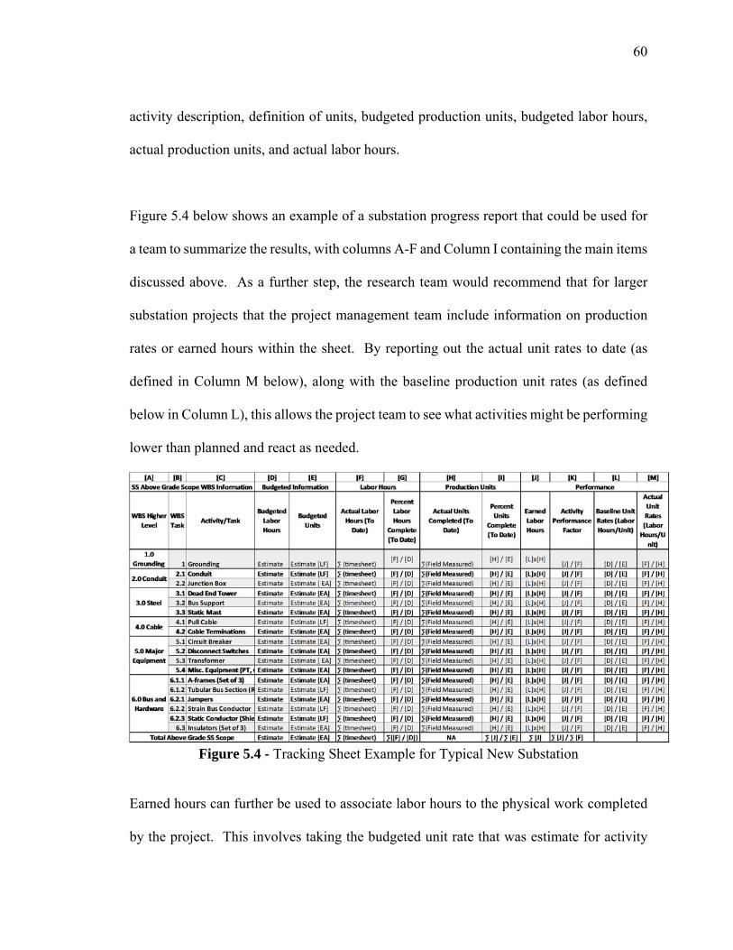
60
activity description, definition of units, budgeted production units, budgeted labor hours,
actual production units, and actual labor hours.
Figure 5.4 below shows an example of a substation progress report that could be used for
a team to summarize the results, with columns A-F and Column I containing the main items
discussed above. As a further step, the research team would recommend that for larger
substation projects that the project management team include information on production
rates or earned hours within the sheet. By reporting out the actual unit rates to date (as
defined in Column M below), along with the baseline production unit rates (as defined
below in Column L), this allows the project team to see what activities might be performing
lower than planned and react as needed.
Figure 5.4 - Tracking Sheet Example for Typical New Substation
Earned hours can further be used to associate labor hours to the physical work completed
by the project. This involves taking the budgeted unit rate that was estimate for activity

61
(Column L) and multiplying it by the actual units completed to date (Column H). Once
the earned hours are calculated (Column J), the team can use the earned hours to determine
the activity performance factor. The activity performance factor (Column K) is calculated
by dividing the Earned Hours (Column J) by the Actual Hours (Column F). If the ratio
value calculated in column K is greater than 1, the activity is producing better than planned.
If the ratio in column K is less than 1, this is an indicator that the activity is producing
worse than planned. The performance values can also be plotted over time to show the
productivity trends for an activity. An example of a Performance Factor Profile is provided
below in Figure 5.5 with the values greater than 1showing production better than planned.
(Hanna 2010)
Figure 5.5 - Performance Factor Profile Example (Hanna 2010)
5.5 Summary The section above highlighted a few other best practices that were identified within the
substation research. Along with establishing S-curves and manpower loading curves to

62
plan and monitor against, the project team should utilize a WBS throughout project
planning and tracking. An example of a typical substation WBS was provided for a new
substation project. The research team recommends that the project team utilize the WBS
to establish a framework for timesheet and progress reporting. In addition, weekly progress
reporting sheets containing actual labor hours, units complete, and other production rates
should be utilized weekly by a project team to monitor project performance.
63
CHAPTER SIX: APPLICATIONS, RECOMMENDATIONS, & CONCLUSION
6.1 Summary Labor control on construction projects is an important project management and team
function to reduce project cost and improve crew production. Successful control of labor
hours during estimating and tracking of a project actuals early on can have a significant
impact on the overall success of a project.
Chapter 1 of the paper discussed the need to establish labor control indicators within the
electrical substation sector via benchmarking tools. The first section of definitions defined
substation project types and function, how they are integrated within the electrical
transmission grid, and provided an overview of the above-grade equipment components.
The second portion of the definitions provided the reader with key construction industry
definitions that were applicable to understanding the research presented. These included
definitions such as production, benchmarking, S-curves, and manpower loading curves.
The problem statement, objectives, scope, and methodology were then all highlighted. The
problem within the electrical industry is that there is a lack of labor hour benchmarks and
control points when compared to other industries. This is becoming more critical to
establish for substation projects as the electrical industry is projected to have approximately
$880 billion of projects within the next two decades. As a result, the goal of this research
was to utilize actual project labor hours and identify typical labor control points. The scope
involved a comprehensive data collection for the above-grade activities of “well-executed”
substation projects from upper Midwest owner completed by two different construction

64
contractors. The methodology used for researching the projects involved developing a
survey, gathering contractor input from survey information and contractor data input
sheets, populating data into excel, analyzing the data for specific model trends, checking
the analysis for adequacy, and reporting of research results. Assumptions were also
documented within this section.
Chapter 2 discussed literature that was reviewed within the industry to help establish the
need and typical use of benchmark indicators. Prior research results established within the
HVAC and WI-DOT were presented to show what has been done in other industries to
date, and how benchmark indicators can be utilized by project teams to improve project
performance. For example, standard manpower loading curves and S-curves have already
been established for mechanical contractors. These can then be used as control points for
estimating and tracking of actual labor hours. The end of this chapter re-iterated the need
for electrical industry labor benchmarks as there is a general lack of research for labor
hours and control indicators in this sector.
Chapter 3 summarized the project data that was collected. A total of 14 projects from an
upper Midwest owner completed by two different contractors had data gathered based on
the survey results and input sheets provided. Specific project characteristics, such as
voltage class, number of labor hours, and type of project were discussed. The major types
of equipment characteristics, such as quantities of circuit breakers and transformer, were
also presented to provide input as to the type of projects for future comparison.
65
Chapter 4 presented the analysis and the model trends developed for the researched
electrical substation data that was discussed in Chapter 3. The analysis provided initial
manpower loading curve and S-curve model trends with R2 values of 0.760 and 0.970
respectively. This was done cumulatively for total above-grade labor, but also broken out
for individual above-grade activities provide input on the sequence and build-up of work
activities. Control points were also added to the typical S-curve generated to provide upper
and lower typical boundaries. In addition to the model curves and control points, typical
breakout of project labor hours by WBS activity and schedule durations were also
established. Boxplots were utilized used for these benchmarks to provide a more visual
average and range of values. The section also provided initial statistical checks for the
model results by conducting regression analysis and residual analysis plots via excel and
Minitab©, and identified recommendation for future statistical research and checking of
the models.
Chapter 5 presented additional best practices that were identified to be used or
recommended for electrical substation projects. Best practices discussed included the need
for a project Work Breakdown Structure (WBS). A WBS example was also provided as a
starting point for a typical new substation project. Methods for gathering actual labor data
and production from the field via timesheets and tracking sheets, along with examples,
were also discussed. The last item within this section went over the typical frequency of
reporting, a progress reporting sheet example, and a few additional reporting items that
could be beneficial to the project team.
66
6.2 Applications
The research findings presented within this paper can be beneficial for electrical substation
practitioners. The research provides typical labor control points that project team members
can utilize to check initial estimates for adequacy and to better control labor on projects.
The results also provide typical, high level control indicators for planning and tracking of
actual labor hours. When planning a project, a contractor can compare their labor plan to
that of the typical S-curve and benchmark indicators and see if they might be too
aggressive. This similar process can also be done during construction by plotting the actual
labor against the typical benchmark indicators. This provides baseline control points for
the project team to identify and react (as needed) to poor performance earlier.
The research also ultimately provides contractors with a mechanism and framework for
establishing their own in-house benchmarks to compare against. It would be highly
recommended for contractors to establish their own in-house benchmarks and control
indicators for their specific niche of projects by using this similar research process
provided. The examples of the WBS along with the timesheet and progress tracking tools
can also be used as starting points if a contractor doesn’t currently utilize these tools. These
can be refined, modified, and improved upon within the organization as projects evolve.
6.3 Recommendations for Future Research There are several recommendations for future research that could benefit the electrical
substation industry. The first major recommendation would be to increase the substation
67
above-grade scope project sample size of projects researched and increase the number of
contractors included as the research here is limited to 14 projects from only two different
contractors. By increasing the project sample size (greater than 30 projects) and adding
more contractors to the database, further statistical analysis and review of the assumptions
made can be done to check the validity of the models and typical results provided. In
addition to adding to the project sample size, projects could be used and tested within the
model as another method to check model validity. It would be recommended that two or
more projects be used and ran within the model to validate this. Along with this, the
additional data might help improve the manpower loading curves R2 value and peak to
average ratios.
Further statistical analysis could also be done to determine which characteristics of the
project are statistically significant, or which activities have more statistical impacts on
project outcomes. For example, it could be researched further to see if location, contract
type, or bus design type have a significant impact on the labor production for these projects.
In addition to this, the research could further be broken out to establish specific manpower
loading curves for individual project types, such as S-curves solely for 138kV new
substation projects based on the specific additional projects that are gathered.
Along with the recommendations above, future research could include the remaining scope
of substation projects. This could include similar research for the below-grade scope of
work activities such as site grading, foundations, stone installation, storm water
management, below-grade conduit installation, etc.. Future research could also look into
68
the breakout percentages for an entire substation project, such as percentage of above-grade
scope to below-grade scope, and typical subcontractors involved. Along with this, typical
equipment (tools) used for constructing substation projects could be researched along with
their typical loading over the project. This could help determine how equipment affects
crew production and project performance.
Further research could also be done with regards to the contract type of the substation
projects. The research presented in this paper, as stated earlier in Chapter 1, was for time
and material contract type. Additional research for other contracts, such as lump sum
contract projects, could be done to see if the control points are in-line with each other. This
could help project teams more specialize their control points for the specific type of project
contract.
Finally, research into Earned Value Management and contractor reporting, similar to that
conducted by Hanna previously in the HVAC industry, could be conducted. This could
include a few case studies of substation project utilizing earned value management,
establish tips for forecasting of labor hours, and identify typical performance factor profiles
for substation activities and substation projects. By having a few case studies researched,
it could be better understood whether or not substation construction labor follows the
typical performance profiles identified in other industries, and how earned value can
improve project forecasting.

69
6.4 Conclusion Due to the large increases in planned capital funds for the electrical grid industry, it is vital
to monitor and control the substation construction resources expended. This paper provides
substation practitioners with initial typical control indicators to better plan and track their
labor performance for above-grade activities, and provides the framework and
recommendations for future additional research in this industry. These control indicators
were developed through comprehensive data collection and analysis of 14 well-executed
substation projects completed in the upper Midwest by two different contractors.
The research from these projects indicate initially that well-executed substation projects
typically consume 30% of the total above-grade labor hours between 0 and 40% of the
project duration. An additional 40% of the labor hours is consumed between 40 and 60%
of the project duration. The final 40% of the project time consumes the remaining 30% of
the above-grade project labor hours. The developed manpower loading curves further
revealed that labor hours typically peak at around 50% project duration with an
approximate peak to average ratio of 180%. Furthermore, data analysis shows that all
above-grade project activities should commence by 30% of project duration. Finally, the
results from the data analysis show that major equipment, bus, and cable installations have
large activity contribution factors, comprising 75% of the substation above-grade labor
hours. Best practices were also discussed to help substation contractors establish consistent
labor reporting and tracking tools.

70
APPENDIX A. REFERENCES
AACE International (AACE). (2011). “AACE International Certified Cost Technician
Primer” AACE International, <http://www.aacei.org/cert/CCT/CCT_Primer.pdf> (June 2015).
Alberta Electric System Operator (AESO).(2014) “Capital Cost Benchmark Study.” Harris Williams,<http://www.aeso.ca/downloads/AESO_Capital_Cost_Benchmark_Study_for_240kV_Projects.pdf> (Oct. 27, 2015).
Barone, Brooke. (2014). “3 Common Steel Structures Found Inside a Substation.” DIS-TRAN High-voltage Specialist, <http://web.distran.com/blog/bid/91964/A-Cheat-Sheet-for-Electrical-Substations-0>. (May 2, 2015).
Bradshaw, George B. (2008). “Establishing a First Class Project Controls Organization for Managing Large Complex Projects.” AACE International Transactions, TCM.01.1-TCM.01.9.
Chen, Mark T. (2006). “Applying Trapezoidal Technique in Resource Management.” AACE International Transactions, PS.03.1-03.7.
Clark, Forrest D. (1985). “Labor Productivity and Manpower Forecasting.” AACE Transactions, A.1.1-A.1.7.
Commonwealth Associates. (2015) <http://www.cai-engr.com/services/images/proj-joppa.jpg> (June 2015).
Construction and Materials Support Center(CMCS). (2012). “Best Practices from WisDOT Mega and ARRA Projects - Statistical Analysis and % Time vs. % Cost Metrics,” University of Wisconsin – Madison, WI.
Fabrimet. (2008). <http://www.fabrimet.com/photos/distri2.jpg> (May 7, 2015).
Frost, Jim. (2014). “Regression Analysis: How to Interpret S, the Standard Error of the Regression.” The Minitab Blog, <http://blog.minitab.com/blog/adventures-in-statistics/regression-analysis-how-to-interpret-s-the-standard-error-of-the-regression> (July 31, 2015).
Gharaibeh, Hani M. (2014). “Cost Control in Mega Projects Using the Delphi Method.” ASCE, pp. 04014024-1 - 04014024-7.
Hanna, Awad S., Peterson, Pehr, and Lee, Min-Jae. (2002). “Benchmarking Productivity Indicators for Electrical/Mechanical Projects.” Journal of Construction Engineering and Management, pp. 331-337.
Hanna, Awad S.. (2010). Providing Vision and Leadership for the Future of the HVAC and Sheet Metal Industry: Project Tracking to Improve Labor Productivity For

71
Mechanical, HVAC, and Sheet Metal Contractors, New Horizon Foundation, Chantilly, Virginia.
Harris Williams & Co..(2014) “Transmission and Distribution Infrastructure.” Harris Williams, <http://www.harriswilliams.com/sites/default/files/industry_reports/ep_td_white_paper_06_10_14_final.pdf?cm_mid=3575875&cm_crmid=e5418e44-29ef-e211-9e7f-00505695730e&cm_medium=email> (May 7, 2015).
Hart, David H. (2007). “The Basics of Design-Assist Contracting.” AIA Best Practices, <http://www.aia.org/aiaucmp/groups/secure/documents/document/aiap029127.pdf> (Oct. 27, 2015).
Heinemann, Jedd, and Scheid, Mark. (2012). “Applying the National Electrical Code to Substation.” Ulteig Engineering, Surveying and Consulting Services, <http://www.ulteig.com/MediaHandler.ashx?id=2342> (May 7, 2015).
Hyde, Marlene M., Orr, John P., and Peek, Michael A.. (2010). “Best Practices by Owners for Controlloing Cost and Schedules on Large Projects.” AACE International Transactions, OWN.06.1 – OWN.06.14.
Kouiden, Redouane. (2012). “Residual Plots Revelations.” The Minitab Blog, <http http://blog.minitab.com/blog/statistics-for-lean-six-sigma/residual-revelations> (July 31, 2015).
Idaho Power Company. (2011). “Appendix B - transmission line and substation components.” Boardman to Hemingway Transmission Line Project, <http://www.boardmantohemingway.com/documents/2011_Nov_POD_AppB.pdf> (May 2, 2015).
JL Malone. (2015). <http://www.jlmalone.com/images/Full%20Size%20Images/wLwELDED%20BUS.jpg> (May 7, 2015).
LGE Electrical Sales. (2015). LGE Electrical Sales. <http://www.lgesales.com/images/projects/01_02.jpg> (June 2, 2015).
Minitab. (2014). “What is a Boxplot” Minitab 17 Support, <http://support.minitab.com/en-us/minitab/17/topic-library/basic-statistics-and-graphs/graphs/graphs-that-compare-groups/boxplots/boxplot/> (July 31, 2015).
National Council on Electric Policy (NCEP). (2004). “Electricity Transmission A Primer.” June 2004. ENERGY.GOV, <http://energy.gov/sites/prod/files/oeprod/DocumentsandMedia/primer.pdf> (Oct. 27, 2015).
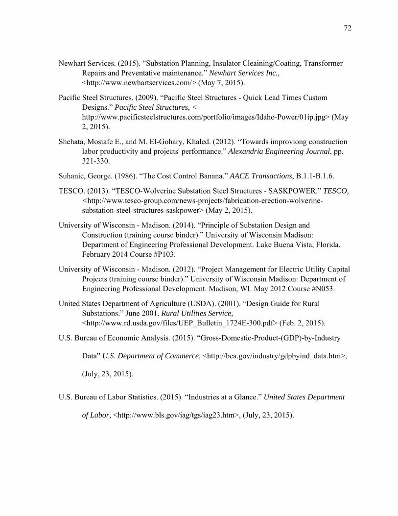
72
Newhart Services. (2015). “Substation Planning, Insulator Cleaining/Coating, Transformer Repairs and Preventative maintenance.” Newhart Services Inc., <http://www.newhartservices.com/> (May 7, 2015).
Pacific Steel Structures. (2009). “Pacific Steel Structures - Quick Lead Times Custom Designs.” Pacific Steel Structures, < http://www.pacificsteelstructures.com/portfolio/images/Idaho-Power/01ip.jpg> (May 2, 2015).
Shehata, Mostafe E., and M. El-Gohary, Khaled. (2012). “Towards improviong construction labor productivity and projects' performance.” Alexandria Engineering Journal, pp. 321-330.
Suhanic, George. (1986). “The Cost Control Banana.” AACE Transactions, B.1.1-B.1.6.
TESCO. (2013). “TESCO-Wolverine Substation Steel Structures - SASKPOWER.” TESCO, <http://www.tesco-group.com/news-projects/fabrication-erection-wolverine-substation-steel-structures-saskpower> (May 2, 2015).
University of Wisconsin - Madison. (2014). “Principle of Substation Design and Construction (training course binder).” University of Wisconsin Madison: Department of Engineering Professional Development. Lake Buena Vista, Florida. February 2014 Course #P103.
University of Wisconsin - Madison. (2012). “Project Management for Electric Utility Capital Projects (training course binder).” University of Wisconsin Madison: Department of Engineering Professional Development. Madison, WI. May 2012 Course #N053.
United States Department of Agriculture (USDA). (2001). “Design Guide for Rural Substations.” June 2001. Rural Utilities Service, <http://www.rd.usda.gov/files/UEP_Bulletin_1724E-300.pdf> (Feb. 2, 2015).
U.S. Bureau of Economic Analysis. (2015). “Gross-Domestic-Product-(GDP)-by-Industry
Data” U.S. Department of Commerce, <http://bea.gov/industry/gdpbyind_data.htm>,
(July, 23, 2015).
U.S. Bureau of Labor Statistics. (2015). “Industries at a Glance.” United States Department
of Labor, <http://www.bls.gov/iag/tgs/iag23.htm>, (July, 23, 2015).

73
Utility Products. (2014). “Circuit Breaker Replacement Project Carries Environmental Benefit." < http://www.utilityproducts.com/articles/print/volume-7/issue-10/product-focus/substation-management-maintenance/circuit-breaker-replacement-project-carries-environmental-benefit.html> (Oct. 27, 2015).
Watts Electric Company. (2015). <http://wattselectriccompany.com/wp-content/uploads/2014/05/KBR-Rural-Public-Power-District-Substations-3.jpg> (May 7, 2015).
Whiteside, Mr. James D. (2006). “Construction Productivity.” AACE International Transactions, EST.08.01-EST.08.08.
Zink, Dwight A.. (1980). “Monitoring the Adequacy of the Amount and Productivity of Engineering and Construction Manpower.” AACE Transactions, C.B.1-C.B.8.
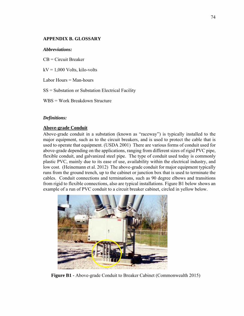
74
APPENDIX B. GLOSSARY
Abbreviations:
CB = Circuit Breaker
kV = 1,000 Volts, kilo-volts
Labor Hours = Man-hours
SS = Substation or Substation Electrical Facility
WBS = Work Breakdown Structure
Definitions:
Above-grade Conduit Above-grade conduit in a substation (known as “raceway”) is typically installed to the major equipment, such as to the circuit breakers, and is used to protect the cable that is used to operate that equipment. (USDA 2001) There are various forms of conduit used for above-grade depending on the applications, ranging from different sizes of rigid PVC pipe, flexible conduit, and galvanized steel pipe. The type of conduit used today is commonly plastic PVC, mainly due to its ease of use, availability within the electrical industry, and low cost. (Heinemann et al. 2012) The above-grade conduit for major equipment typically runs from the ground trench, up to the cabinet or junction box that is used to terminate the cables. Conduit connections and terminations, such as 90 degree elbows and transitions from rigid to flexible connections, also are typical installations. Figure B1 below shows an example of a run of PVC conduit to a circuit breaker cabinet, circled in yellow below.
Figure B1 - Above-grade Conduit to Breaker Cabinet (Commonwealth 2015)

75
Above-grade Grounding Above-grade grounding is also needed for the above-grade scope of work. This is done to ground steel structures, such as those for equipment stands or bus supports, ground major equipment such as circuit breakers, and ground perimeter fencing. (USDA 2001) Above-grade grounding, which typically consists of 4/0 copper, is tied to the steel structure and then connected to the installed ground grid that is part of the below grade substation work. (USDA 2001) Grounding is used within the substation to provide human safety by allowing individuals within the substation to not be exposed to an electric shock. Along with this, the grounding system is used to take electrical currents from faults to the ground where it is dissipated and also provides reduction in damages caused by lightning strikes. (USDA 2001) Figure B2 below shows an example of structure steel being grounded with copper (circled below in figure).
Figure B2 - Above-grade Grounding on Steel Structure (Watts Electric 2015)

76
Benchmarking Benchmarking of past data includes gathering project cost metrics and labor to establish high level milestones and control points. The benchmark data can then be used as inputs or verification tools to check against estimates or actuals. (Bradshaw 2008) Benchmarking can also include research and development of standard manpower loading curves and S-curves for projects to identify project milestones (benchmark indicators) and or labor control points. (Hanna 2010)
Benchmark Indicators Benchmarking indicators, or benchmark control points, are the key outputs from benchmarking that can be used to validate project estimates and actuals. This process involves utilizing past project data, such as labor hours, to establish typical project trends. The labor hour trends established can then be used by future project teams to serve as control points within the planning stage, and also used as monitoring of actual construction progress.
Buswork Installation (bus - rigid and strain, and jumpers) Buswork (or bus) are the main structural components used in the substation for carrying the electrical current thru the substation facility. As discussed earlier, buswork can be arranged in different configurations to create several substation layout options. This includes ring bus configurations, breaker-and-a-half, single bus, etc. There are two main types of bus used within the different substations facility types, which include rigid and strain bus. Rigid bus (rigid conductors), as shown in Figure B3 below, are typically used in low profile type substations with lower steel structure supports. (USDA 2001) Rigid bus can be found within the site in different shapes and sizes, such as with the use of tubular aluminum as shown below in Figure B3. Selection of the size and type of bus used within the system depends on the current capacity needed for the design of the substation. (USDA 2001)
Figure B3 - Rigid Bus within a Low-profile Substation (JL Malone 2015)

77
Strain bus are also used for carrying current in the substation facility. The strain bus is typically composed of flexible conductors, such aluminum strand conductor. (USDA 2001) The size of the wire, along with the type of conductive material used all impact the overall ampacity of the substation. (USDA 2001) Strain conductors are typical within a lattice box structure to carry the electrical current within the structure. Figure B4 below shows an example of strain conductor used for carrying current within the box structure. Flexible conductors are also commonly used as “jumpers” within a substation. Similar to strain bus, jumpers consist of electrical conductor (such as aluminum strands of conductor) to serve as the electrical path connection from the rigid bus to the major piece of equipment. Figure B5 below shows jumper material used to connect from the main bus to a circuit breaker.
Figure B4 - Lattice Box Structure with Strain Bus (Fabrimet 2008)
Figure B5 - Jumpers to Circuit Breaker (University of Wisconsin-Madison)

78
Circuit Breakers (High-voltage Circuit Breakers, (CB)) A Circuit Breaker (CB), as defined in the RUS design for high-voltage applications, is a “device that closes and interrupts (opens) an electric circuit between separable contacts under both load and fault conditions.” (USDA 2001) Figure B6 below shows a typical CB commonly seen inside a substation facility. This breaker type uses SF6 gas as the medium to interrupt the electrical current, whereas existing breakers typically used oil filled tanks. A CB is commonly seen for each phase, sits on a concrete foundation, and typically has disconnect switches on each side of the breaker for visual isolation. (USDA 2001)
Figure B6 - High-voltage Circuit Breaker; Gas Type (Utility Products 2014)
Control Cable (or cable) Installation of control cable is another above-grade component of substation facilities. Within a substation yard, the above-grade scope of work involves pulling cable thru the conduit from the equipment cabinet and terminating it within the control house (equipment enclosure building). Control cable serves the function of sending metering and protection information for the major piece of equipment, and for providing backup DC power to the equipment. (Idaho Power Company 2011) Copper conductor is typically used within substations as the terminations can be made fairly easy with it.
Distribution Step-Down Substation Distribution step-down substation facility is another type of substation found on the electrical grid system. These facilities are a key connection point within the electrical grid system to step down the high-voltage on the transmission line (69kV and greater) to the distribution voltage (12.5kV typical). They contain power transformers to step-down the voltage as noted above, and feeder exits on the distribution side. The distribution feeders provide multiple sources of power to the distribution facilities. (University of Wisconsin-Madison 2014) Figure B7 below illustrates this configuration in a plan view form, with the incoming/outgoing transmission voltage at 138kV being step-down via a power transformer to the distribution voltage. (University of Wisconsin-Madison 2014) This is the final transmission facility in the high-voltage grid system and the rest of power delivery is handled by the distribution system.

79
Figure B7 - One-Line example of a 138kV to Distribution Step-Down Substation (University of Wisconsin-Madison 2014)
Power Transformer (XFRM) A power transformer (XFRM) is a 3-phase electrical component that uses various windings to change (step-down or step-up) the voltage from one level to another, such as going from 138kV to 69kV. (USDA 2001) Figure B8 below shows a typical XFRM that might commonly be seen inside a substation facility. As seen in Figure B8 below, XFRMs are typically one of the largest pieces of equipment within the substation site and sit on a large concrete foundation pad. They contain large fans for cooling and dissipating heat, and have large tanks for oil to be used as a cooling mechanism as well. (USDA) Along with this, the XFRM has an oil containment system (typical sunken foundation with metal grate on top) for mitigating environmental impacts due to potential oil spill.
Figure B8 - Example of a High-voltage Power Transformer (Newhart Services 2015)

80
Production (Productivity) Productivity, or production, is generally defined within the construction industry as the output of work per a measured amount of labor hours. (Shehata 2012) It can also be seen or known in the industry as a unit rate, where labor hours are described per unit of installation (Labor hours/ Units). (Shehata 2012)
Step-down Substation (Change in Voltage Substation) Step-down substation is also commonly known as a change in voltage substation. These facilities are very common in high-voltage (69-345kV) transmission applications. The primary function of these facilities is to change the voltage along the transmission line path from one voltage level, such as higher voltage of 345kV on the primary side, down to 138kV level on the secondary side via a 3-phase power transformer. Figure B9 below illustrates this configuration in a plan view form with the power transformer dropping the voltage down from 345kV to 138kV.
Figure B9 - One-Line example of a 345 to 138kV Step-Down Substation (University of Wisconsin-Madison 2014)
Support Steel (Steel Stand and Lattice Steel Structures) Steel structure types are primarily used within the substation facility to hold up electrical equipment. Other materials can be used, but steel is typically the most commonly used. There are several design functions that the steel supports provide. First, it it provides overall structure support to withstand appropriate structural loads (wind, ice, etc). Second, structural steel supports are used to provide clearances from the equipment to the ground or other objects. Also, steel can be galvanized which prevents corrosion and longer lifespan. (University of Wisconsin-Madison 2014) A few examples of the different structural steel types used within a substation facility are shown below. Figure B10 shows common steel support stands for a rigid bus design. The steel supports shown in the picture are used to hold up the rigid bus (circled in Figure B10). Figure B11 below also shows stands being used tp hold up smaller equipment items such as disconnect switches (circled in the figure) or other components. (USDA 2001)
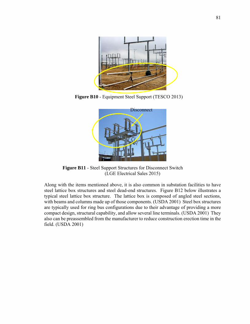
81
Figure B10 - Equipment Steel Support (TESCO 2013)
Figure B11 - Steel Support Structures for Disconnect Switch (LGE Electrical Sales 2015)
Along with the items mentioned above, it is also common in substation facilities to have steel lattice box structures and steel dead-end structures. Figure B12 below illustrates a typical steel lattice box structure. The lattice box is composed of angled steel sections, with beams and columns made up of those components. (USDA 2001) Steel box structures are typically used for ring bus configurations due to their advantage of providing a more compact design, structural capability, and allow several line terminals. (USDA 2001) They also can be preassembled from the manufacturer to reduce construction erection time in the field. (USDA 2001)
Disconnect
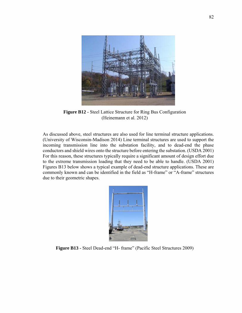
82
Figure B12 - Steel Lattice Structure for Ring Bus Configuration (Heinemann et al. 2012)
As discussed above, steel structures are also used for line terminal structure applications. (University of Wisconsin-Madison 2014) Line terminal structures are used to support the incoming transmission line into the substation facility, and to dead-end the phase conductors and shield wires onto the structure before entering the substation. (USDA 2001) For this reason, these structures typically require a significant amount of design effort due to the extreme transmission loading that they need to be able to handle. (USDA 2001) Figures B13 below shows a typical example of dead-end structure applications. These are commonly known and can be identified in the field as “H-frame” or “A-frame” structures due to their geometric shapes.
Figure B13 - Steel Dead-end “H- frame” (Pacific Steel Structures 2009)
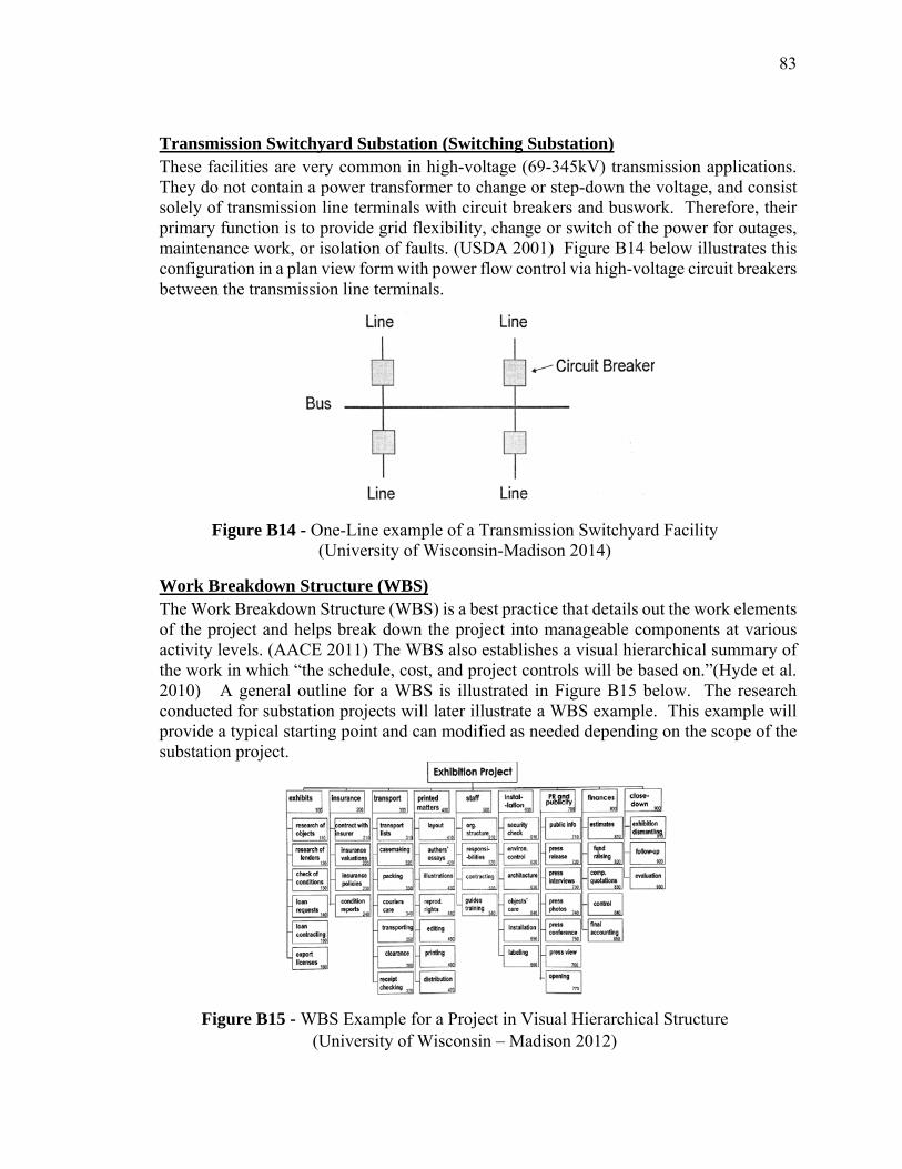
83
Transmission Switchyard Substation (Switching Substation) These facilities are very common in high-voltage (69-345kV) transmission applications. They do not contain a power transformer to change or step-down the voltage, and consist solely of transmission line terminals with circuit breakers and buswork. Therefore, their primary function is to provide grid flexibility, change or switch of the power for outages, maintenance work, or isolation of faults. (USDA 2001) Figure B14 below illustrates this configuration in a plan view form with power flow control via high-voltage circuit breakers between the transmission line terminals.
Figure B14 - One-Line example of a Transmission Switchyard Facility (University of Wisconsin-Madison 2014)
Work Breakdown Structure (WBS) The Work Breakdown Structure (WBS) is a best practice that details out the work elements of the project and helps break down the project into manageable components at various activity levels. (AACE 2011) The WBS also establishes a visual hierarchical summary of the work in which “the schedule, cost, and project controls will be based on.”(Hyde et al. 2010) A general outline for a WBS is illustrated in Figure B15 below. The research conducted for substation projects will later illustrate a WBS example. This example will provide a typical starting point and can modified as needed depending on the scope of the substation project.
Figure B15 - WBS Example for a Project in Visual Hierarchical Structure (University of Wisconsin – Madison 2012)

84
APPENDIX C. PROJECT SURVEY TEMPLATE (Microsoft Word File)
Substation Electrical Contractor Construction ‐ High-voltage Substation Projects for “Electrical Scope of Work”. ‐ “Electrical” contractor scope of work defined as: o Not including grading, foundations, site work, and other below grade activities such as installing conduit
and trenches. o Not including Transmission line scope for the project.
Instructions This survey is for the Construction phase of the substation project only, starting at the end of below grade work (foundations and grading) and concluding with final construction in-service and commissioning. This therefore covers only the electrical scope of work for the project and doesn’t include any below grade activities. There are 7 sections in the survey, with the summary of each section bulleted below. The items noted with an “*” in the survey include additional information and description at the base of the survey. It is preferred that this survey form be filled out based on a “new large High-voltage Substation construction project” for projects considered good or better than average for you company. (High-voltage meaning >69kV, and large meaning > 8,000 labor hours, “good” project characterized within +10 -30 % labor hours). (Need to define “good” yet further”
1. General Information 2. Project Characteristics 3. Project Labor, Cost, and Schedule Data – Baseline and Actual Data 4. Project Change Order 5. Contract Document and Contract Type 6. Project Management: Resource Tracking and Physical Tracking 7. Construction Labor Crew Makeup
The intent of the survey is to be completed by the members of the project team that were managing the on-site construction. Questions should be answered to the best of your team’s ability, with data provided to support results as noted in the survey. (Specifically labor hours over the life of the project for manpower information)
All data collected and provided for the survey that the team member and organizations provide is confidential. The data will not be viewed by any party other than those of the University of Wisconsin Construction Engineering and Management (CEM) Research staff members. Should you have any questions with the survey, please contact Dr. Hanna via email ([email protected]) or by phone xxxxx. The UW CEM Research staff members thanks you for your participation in this initiative to gather substation electrical construction data.

85
SECTION 1: GENERAL INFORMATION Person completing this part of the survey: Your Name: Address: Your Company Name: Your Cumulative Years of Experience in Capital Projects: Telephone Fax Email Would you prefer correspondence by email or telephone (please circle one)? What is the best time to reach you (indicate time zone)? What position do you hold within your construction company?
Owner President Vice president Superintendent Project manager Other (specify) ________
Owner Company Name: Project Construction Location: City: _________, State: ______, Project Location Type: Urban_____ Rural______ Other_______ Lead Construction Contractor: Name: ____Contractor ____State:
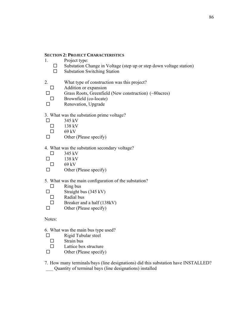
86
SECTION 2: PROJECT CHARACTERISTICS 1. Project type:
Substation Change in Voltage (step up or step down voltage station) Substation Switching Station
2. What type of construction was this project? Addition or expansion Grass Roots, Greenfield (New construction) (~80acres) Brownfield (co-locate)
Renovation, Upgrade 3. What was the substation prime voltage?
345 kV 138 kV 69 kV
Other (Please specify)
4. What was the substation secondary voltage? 345 kV 138 kV 69 kV
Other (Please specify)
5. What was the main configuration of the substation? Ring bus
Straight bus (345 kV) Radial bus Breaker and a half (138kV)
Other (Please specify) Notes: 6. What was the main bus type used?
Rigid Tubular steel Strain bus Lattice box structure
Other (Please specify) 7. How many terminals/bays (line designations) did this substation have INSTALLED? ___ Quantity of terminal bays (line designations) installed

87
8. How many terminals/bays (line designations) did this substation have designed total for FUTURE? ____ Quantity of terminal bays (line designations) future
9. How many large voltage step-up/step-down transformers did this substation have? ___ Quantity of large voltage transformers
None, this was a switching station Other (Please specify)
10. How many circuit breakers did this project have? ___ Quantity of breakers
11. Was any part of your project executed on an existing operating unit/brownfield site?
Yes X No If yes, was this Partial site or Majority of Site? Partial Majority
12. How many OSHA recordable occurred on this project?
0 1-3 3-6 6+ SECTION 3: PROJECT LABOR, COST, AND SCHEDULE DATA
1. The contract budgeted crew labor hours7 at the notice to proceed for the project:
(Note this is for “electrical installation scope only”: installing steel supports/structures, setting equipment, setting control house, wiring, terminations, grounding, installing above-grade conduit. Not including any below grade work of trenching for conduit, installation of duct banks, installing conduit in trenway/ducts, civil work of foundations, grading, and any removals hours and any PMO or superintendent/GF costs. Direct crew labor hours only, those procuring the work no oversight)
Direct electrical scope baseline labor hours hrs. * Please provide example of construction estimate if available. 2. The actual labor hours utilized at completion of the project, including change orders:
7 Contract budgeted labor hours – The total estimated labor hours (man-hours) that the contractor used to allocate labor resources.

88
(Note this is for “electrical scope only”: installing steel supports/structures, setting equipment, setting control house, wiring control house, etc., not including below grade work of conduit install/trenway/ducts, foundations)
Actual electrical scope direct labor hour’s hrs. Please provide example of budget vs. actual that was used for this data if available
3. The estimated planned project duration at contract award for electrical scope: (From electrical start (Setting Steel Structures Start, receive and assemble transformers, or setting control house if new house set first) to construction completion of electrical scope planned construction calendar weeks __ planned electrical construction start
__ planned electrical construction finish (construction of electrical scope complete)
4. The actual project duration at completion for electrical scope: (From electrical start (Setting Steel Structures Start, receive and assemble transformers, or setting control house if new house set first) to construction completion of electrical scope) Actual construction calendar weeks ____ Actual construction start ____ Actual construction finish (in service date) 5. The estimated project construction cost for electrical work: (Labor and Equipment Only (L&E)) Estimate electrical scope L&E construction *Note, please provide cost data sheet or example of estimate if available Excluding foundation, site work, grading (below grade scope) 6. The actual electrical project L&E construction cost: (Labor and Equipment Only) Actual electrical scope L&E construction $ (excluding foundation, site work, grading (below grade scope)) *Note, please provide cost data sheet of budget/actual if available SECTION 4. PROJECT CHANGE ORDER SECTION 1. The total submitted requested change order labor hours for electrical scope of work? (Requests documenting the changes but not approval yet to the Purchase Order) Direct labor hours requested for changes hrs.
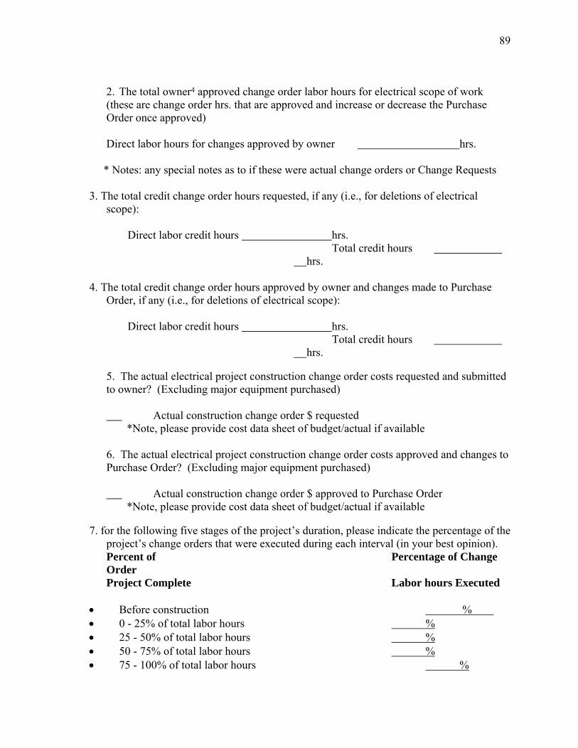
89
2. The total owner4 approved change order labor hours for electrical scope of work (these are change order hrs. that are approved and increase or decrease the Purchase Order once approved) Direct labor hours for changes approved by owner hrs. * Notes: any special notes as to if these were actual change orders or Change Requests
3. The total credit change order hours requested, if any (i.e., for deletions of electrical
scope): Direct labor credit hours hrs. Total credit hours
hrs.
4. The total credit change order hours approved by owner and changes made to Purchase Order, if any (i.e., for deletions of electrical scope):
Direct labor credit hours hrs. Total credit hours
hrs. 5. The actual electrical project construction change order costs requested and submitted to owner? (Excluding major equipment purchased) Actual construction change order $ requested
*Note, please provide cost data sheet of budget/actual if available 6. The actual electrical project construction change order costs approved and changes to Purchase Order? (Excluding major equipment purchased) Actual construction change order $ approved to Purchase Order
*Note, please provide cost data sheet of budget/actual if available
7. for the following five stages of the project’s duration, please indicate the percentage of the project’s change orders that were executed during each interval (in your best opinion). Percent of Percentage of Change Order Project Complete Labor hours Executed
Before construction % 0 - 25% of total labor hours % 25 - 50% of total labor hours % 50 - 75% of total labor hours % 75 - 100% of total labor hours %

90
(Total percentages should sum to 100 %.)
8. Number of owner initiated change items: #
9. Number of contractor initiated change items: #
11. Number of change items requested: # 12. Number of change items approved for PO Change by Owner: # 13. The following are possible reasons for change orders. For each reason that applies to your project, indicate the percent of actual executed labor hours of change orders.
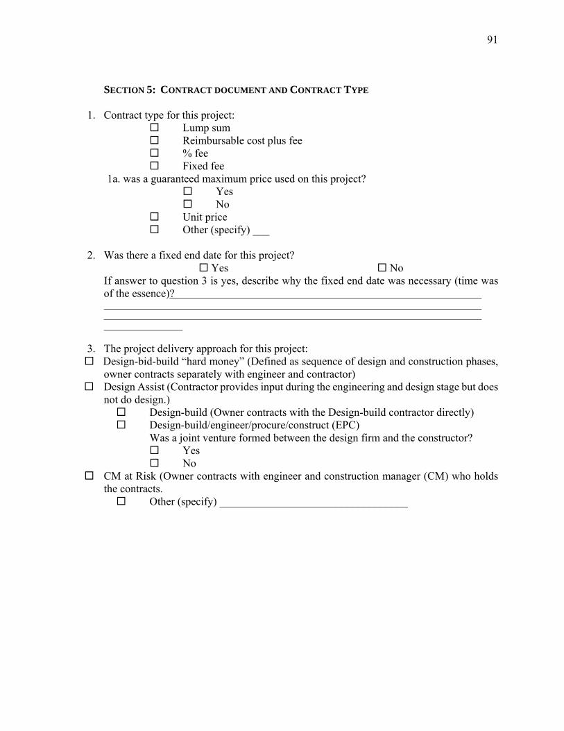
91
SECTION 5: CONTRACT DOCUMENT AND CONTRACT TYPE
1. Contract type for this project: Lump sum Reimbursable cost plus fee % fee Fixed fee
1a. was a guaranteed maximum price used on this project? Yes No Unit price Other (specify) ___
2. Was there a fixed end date for this project?
Yes No If answer to question 3 is yes, describe why the fixed end date was necessary (time was of the essence)?
3. The project delivery approach for this project: Design-bid-build “hard money” (Defined as sequence of design and construction phases,
owner contracts separately with engineer and contractor) Design Assist (Contractor provides input during the engineering and design stage but does
not do design.) Design-build (Owner contracts with the Design-build contractor directly) Design-build/engineer/procure/construct (EPC)
Was a joint venture formed between the design firm and the constructor? Yes No CM at Risk (Owner contracts with engineer and construction manager (CM) who holds
the contracts. Other (specify) __________________________________
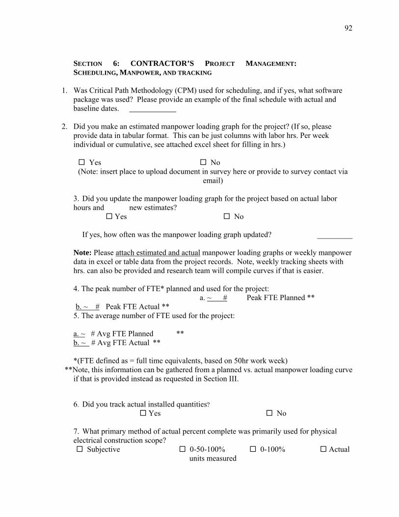
92
SECTION 6: CONTRACTOR’S PROJECT MANAGEMENT:
SCHEDULING, MANPOWER, AND TRACKING
1. Was Critical Path Methodology (CPM) used for scheduling, and if yes, what software package was used? Please provide an example of the final schedule with actual and baseline dates.
2. Did you make an estimated manpower loading graph for the project? (If so, please
provide data in tabular format. This can be just columns with labor hrs. Per week individual or cumulative, see attached excel sheet for filling in hrs.) Yes No (Note: insert place to upload document in survey here or provide to survey contact via
email) 3. Did you update the manpower loading graph for the project based on actual labor hours and new estimates? Yes No If yes, how often was the manpower loading graph updated? _________ Note: Please attach estimated and actual manpower loading graphs or weekly manpower data in excel or table data from the project records. Note, weekly tracking sheets with hrs. can also be provided and research team will compile curves if that is easier. 4. The peak number of FTE* planned and used for the project: a. ~ # Peak FTE Planned ** b. ~ # Peak FTE Actual **
5. The average number of FTE used for the project: a. ~ # Avg FTE Planned ** b. ~ # Avg FTE Actual ** *(FTE defined as = full time equivalents, based on 50hr work week)
**Note, this information can be gathered from a planned vs. actual manpower loading curve if that is provided instead as requested in Section III.
6. Did you track actual installed quantities? Yes No
7. What primary method of actual percent complete was primarily used for physical electrical construction scope? Subjective 0-50-100% 0-100% Actual
units measured

93
8. Did you track performance productivity (input [labor hours]/output [units installed]) for the project?
Yes No SECTION 7: CONSTRUCTION LABOR AND CREW MAKEUP
1. What were the approximate Apprentice to Journeyman crew makeup ratios? (observe time sheet data for this) 0-25% 30-65% 75-100%
2. Was a General Forman used on the project? Yes No (Check percentage utilized below)
0-25% 30-65% 75-100%
3. Was a Superintendent used on the project? Yes No (Check percentage utilized below) 0-25% 30-65% 75-100%
4. What was the typical foreman to craft ratio used on the project: (actual observed or typical for project calculated as ratio = foreman hrs. /total electrical crew hrs.)
<5:1 6:1 ~ 8:1 9:1 ~ 12:1 >13:1 Specific Notes:
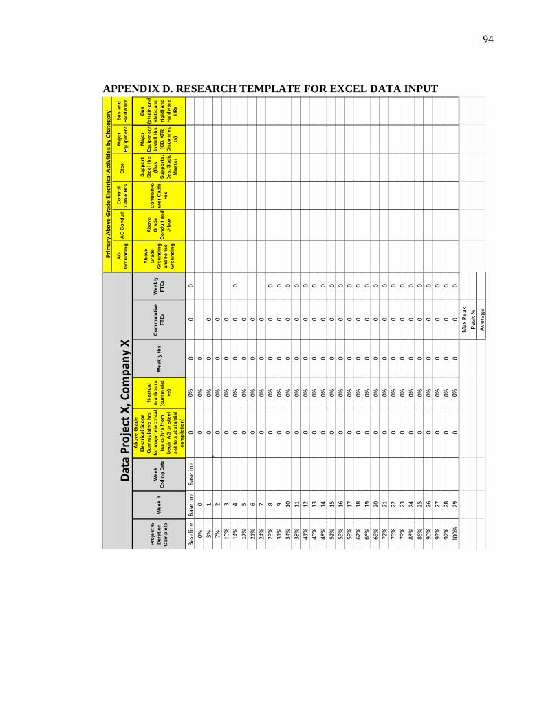
94
APPENDIX D. RESEARCH TEMPLATE FOR EXCEL DATA INPUT
AG
G
rou
nd
ing
AG
Co
nd
uit
Co
ntr
ol
Cab
le H
rsS
tee
lM
ajo
r Eq
uip
me
nt
Bu
s a
nd
H
ard
war
e
Pro
ject
%
Du
rati
on
C
om
ple
teW
ee
k #
We
ek
En
din
g D
ate
Ab
ove
Gra
de
El
ect
rica
l Sco
pe
C
um
mu
lati
ve h
rs
for
maj
or
ele
ctri
cal
tas
ks
(hrs
fro
m
be
gin
AG
or
ste
el
se
t to
su
bs
tan
tial
co
mp
leti
on
)
% a
ctu
al
man
ho
urs
(c
um
mu
lati
ve)
We
ek
ly H
rsC
um
mu
lati
ve
FTEs
We
ek
ly
FTEs
Ab
ove
G
rad
e
Gro
un
din
g
and
Fe
nce
G
rou
nd
ing
Ab
ove
G
rad
e
Co
nd
uit
an
d
J-b
ox
Co
ntr
ol/P
ow
er
Cab
le
Hrs
Su
pp
ort
S
tee
l Hrs
(B
us
S
up
po
rts
, D
es
, Sta
tic
Mas
ts)
Maj
or
Equ
ipm
en
t In
sta
ll H
rs
(CB
, XFR
, D
isco
nn
ec
ts)
Bu
s
(str
ain
an
d
sta
tic
and
ri
gid
) an
d
Har
dw
are
H
Rs
Baseline
Baseline
Baseline
00%
00
0
0%0
00%
0
3%1
00%
00
7%2
00%
00
10%
30
0%0
0
14%
40
0%0
00
17%
50
0%0
0
21%
60
0%0
0
24%
70
0%0
0
28%
80
0%0
00
31%
90
0%0
00
34%
100
0%0
00
38%
110
0%0
00
41%
120
0%0
00
45%
130
0%0
00
48%
140
0%0
00
52%
150
0%0
00
55%
160
0%0
00
59%
170
0%0
00
62%
180
0%0
00
66%
190
0%0
00
69%
200
0%0
00
72%
210
0%0
00
76%
220
0%0
00
79%
230
0%0
00
83%
240
0%0
00
86%
250
0%0
00
90%
260
0%0
00
93%
270
0%0
00
97%
280
0%0
00
100%
290
0%0
00
Max Peak
Peak %
Average
Data Project X, Compan
y X
Primary Above
Grade Electrical A
ctivities by Chategory

95
APPENDIX E. SUMMARY OF EXCEL DATA – PROJECT CHARACTERISTICS
LocationProject Type
New, Addition or expansion
Primary Voltage
RuralChange in Voltage
Grass Roots (new)
345 kV
RuralSubstation Switching
Grass Roots (new)
138 kV
RuralChange in Voltage
Addition or expansion
138 kV
UrbanSubstation Switching
Addition or expansion
345 kV
RuralChange in Voltage
Grass Roots (new)
138 kV
UrbanSubstation Switching
Addition or expansion
138 kV
RuralSubstation Switching
Grass Roots (new)
69 kV
RuralChange in Voltage
Addition or expansion
345 kV
RuralChange in Voltage
Grass Roots (new)
138 kV
RuralChange in Voltage
Grass Roots (new)
138 kV
RuralChange in Voltage
Grass Roots (new)
138 kV
RuralChange in Voltage
Addition or expansion
138 kV
RuralChange in Voltage
Addition or expansion
138 kV
RuralSubstation Switching
Grass Roots (new)
345 kV

96
APPENDIX F. MINITAB© RESULTS
Appendix F1. Manpower Loading Curve Minitab© Analysis and Report
Polynomial Regression Analysis: y versus x The regression equation is y = - 0.1003 + 7.897 x - 9.671 x^2 + 1.774 x^3 S = 0.420094 R-Sq = 72.8% Analysis of Variance Source DF SS MS F P Regression 3 47.2328 15.7443 89.21 0.000 Error 100 17.6479 0.1765 Total 103 64.8808 Sequential Analysis of Variance Source DF SS F P Linear 1 0.1150 0.18 0.671 Quadratic 1 46.9153 265.45 0.000 Cubic 1 0.2025 1.15 0.287
1.00.80.60.40.20.0
300.00%
200.00%
100.00%
0.00%
-100.00%
S 0.420094R-Sq 72.8%
x
y
Regression95% CI95% PI
Manpower Loading Plots for Substation Above-Grade y = - 0.1003 + 7.897 x
- 9.671 x^2 + 1.774 x^3
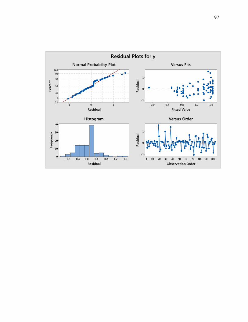
97
10-1
99.999
90
50
10
1
0.1
Residual
Perc
ent
1.61.20.80.40.0
1
0
-1
Fitted Value
Resi
dual
1.61.20.80.40.0-0.4-0.8
40
30
20
10
0
Residual
Freq
uenc
y
1009080706050403020101
1
0
-1
Observation Order
Resi
dual
Normal Probability Plot Versus Fits
Histogram Versus Order
Residual Plots for y

98
Appendix F2. S-Curve Minitab© Analysis and Reports Minitab© Results
The regression equation is y = - 0.00122 + 0.2513 x + 2.374 x^2 - 1.629 x^3 S = 0.0638109 R-Sq = 97.3% Analysis of Variance Source DF SS MS F P Regression 3 13.3365 4.44549 1091.77 0.000 Error 91 0.3705 0.00407 Total 94 13.7070 Sequential Analysis of Variance Source DF SS F P Linear 1 13.1538 2211.38 0.000 Quadratic 1 0.0070 1.18 0.281 Cubic 1 0.1757 43.14 0.000
100%80%60%40%20%0%
125.00%
100.00%
75.00%
50.00%
25.00%
0.00%
S 0.0638109R-Sq 97.3%
x: Percentage of Project Duration y: P
erce
ntag
e of
Cum
mul
ativ
e Pr
ojec
t Lab
or H
ours
Regression95% CI95% PI
Cummulative S-Curve Plots for Above-Grade Substation Constructiony = - 0.00122 + 0.2513 x+ 2.374 x^2 - 1.629 x^3
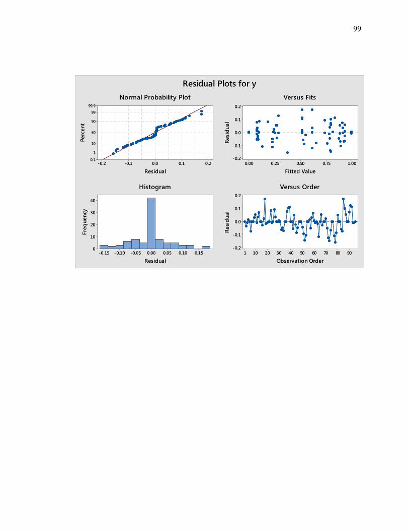
99
0.20.10.0-0.1-0.2
99.999
90
50
10
1
0.1
Residual
Perc
ent
1.000.750.500.250.00
0.2
0.1
0.0
-0.1
-0.2
Fitted Value
Resi
dual
0.150.100.050.00-0.05-0.10-0.15
40
30
20
10
0
Residual
Freq
uenc
y
9080706050403020101
0.2
0.1
0.0
-0.1
-0.2
Observation Order
Resi
dual
Normal Probability Plot Versus Fits
Histogram Versus Order
Residual Plots for y
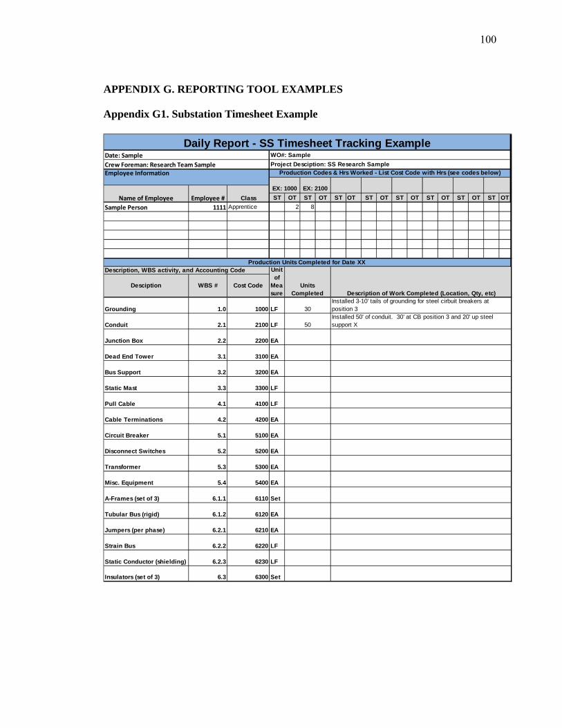
100
APPENDIX G. REPORTING TOOL EXAMPLES
Appendix G1. Substation Timesheet Example
Employee Information
ST OT ST OT ST OT ST OT ST OT ST OT ST OT ST OT
Sample Person 1111 Apprentice 2 8
Desciption WBS # Cost Code
Grounding 1.0 1000 LF
Conduit 2.1 2100 LF
Junction Box 2.2 2200 EA
Dead End Tower 3.1 3100 EA
Bus Support 3.2 3200 EA
Static Mast 3.3 3300 LF
Pull Cable 4.1 4100 LF
Cable Terminations 4.2 4200 EA
Circuit Breaker 5.1 5100 EA
Disconnect Switches 5.2 5200 EA
Transformer 5.3 5300 EA
Misc. Equipment 5.4 5400 EA
A-Frames (set of 3) 6.1.1 6110 Set
Tubular Bus (rigid) 6.1.2 6120 EA
Jumpers (per phase) 6.2.1 6210 EA
Strain Bus 6.2.2 6220 LF
Static Conductor (shielding) 6.2.3 6230 LF
Insulators (set of 3) 6.3 6300 Set
Daily Report - SS Timesheet Tracking ExampleWO#: Sample
Project Desciption: SS Research Sample
Date: Sample
Crew Foreman: Research Team Sample
Unit of
Measure
Units Completed Description of Work Completed (Location, Qty, etc)
Name of Employee Employee # Class
EX: 1000 EX: 2100
Production Codes & Hrs Worked - List Cost Code with Hrs (see codes below)
30
50
Installed 3-10' tails of grounding for steel cirbuit breakers at position 3Installed 50' of conduit. 30' at CB position 3 and 20' up steel support X
Description, WBS activity, and Accounting CodeProduction Units Completed for Date XX
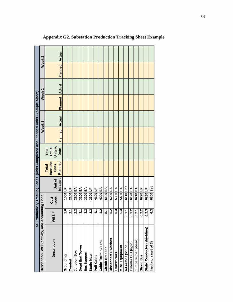
101
Appendix G2. Substation Production Tracking Sheet Example
De
scri
pti
on
WB
S #
Co
st
Co
de
To
tal
Ba
seli
ne
U
nit
s P
lan
ne
d
Planned
Actual
Planned
Actual
Planned
Actual
Gro
un
din
g1.
010
00L
F
Co
nd
uit
2.1
2100
LF
Jun
ctio
n B
ox
2.2
2200
EA
De
ad
En
d T
ow
er
3.1
3100
EA
Bu
s S
up
po
rt3.
232
00E
A
Sta
tic
Ma
st3.
333
00L
F
Pu
ll C
ab
le4.
141
00L
F
Ca
ble
Te
rmin
ati
on
s4.
242
00E
A
Cir
cuit
Bre
ake
r5.
151
00E
A
Dis
con
ne
ct S
wit
che
s5.
252
00E
A
Tra
nsf
orm
er
5.3
5300
EA
Mis
c. E
qu
ipm
en
t5.
454
00E
A
A-F
ram
es
(se
t o
f 3)
6.1.
161
10S
et
Tu
bu
lar
Bu
s (r
igid
)6.
1.2
6120
EA
Jum
pe
rs (
pe
r p
ha
se)
6.2.
162
10E
A
Str
ain
Bu
s6.
2.2
6220
LF
Sta
tic
Co
nd
uct
or
(sh
ield
ing
)6.
2.3
6230
LF
Insu
lato
rs (
set
of
3)6.
363
00S
et
SS
Pro
du
ctiv
ity
Tra
ckin
g S
he
et
(U
nit
s C
om
ple
ted
an
d P
lan
ne
d U
nit
s E
xa
mp
le S
he
et)
Week 1
Week 2
Week 3
De
scri
pti
on
, W
BS
act
ivit
y, a
nd
Acc
ou
nti
ng
Co
de
Un
it o
f M
ea
sure
To
tal
Act
ua
l U
nit
s to
D
ate
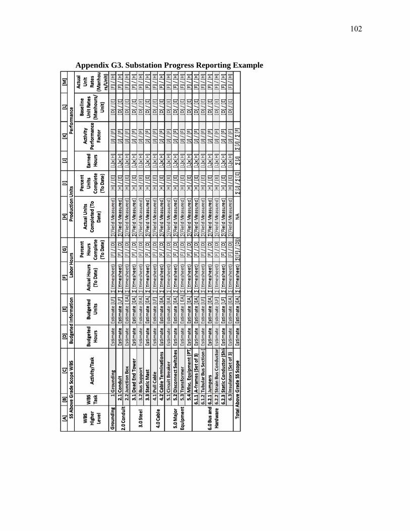
102
Appendix G3. Substation Progress Reporting Example


