

Bifurcations in Forced Taylor–Couette Flow
Anthony John Youd
Thesis submitted for the degree of
Doctor of Philosophy
NEWCASTLE
UN IVERS ITY OF
School of Mathematics and Statistics
University of Newcastle upon Tyne
Newcastle upon Tyne
United Kingdom
November 2005

Acknowledgements
Firstly, and above all, I would like to thank my supervisor Carlo Barenghi for his
guidance and help over the past three years. I would also like to thank Ashley Willis
for the use of his numerical code — many of the results in this thesis would not have
been possible without it.
I would also like to acknowledge the financial support of the Engineering and Phys-
ical Sciences Research Council and the School of Mathematics and Statistics.
Finally, I would like to thank my family for all their support and encouragement
during my time at University.
In memory of Doreen Youd
Abstract
The transition from azimuthal Couette flow to a cellular Taylor vortex flow pattern has
long been recognised as a cornerstone of hydrodynamic stability theory since the work
of Taylor in 1923.
Much of the work done has been concerned with steadily rotating cylinders and
the various transitions that take place as the rotation rate of the cylinders is steadily
increased. This thesis will be concerned with forced variations of the Taylor–Couette
problem.
In the simplest case of a temporally forced geometry where the outer cylinder is
fixed and the inner cylinder oscillates harmonically about a zero mean we shall examine
the flow patterns that can occur and reveal the existence of new axisymmetric and non-
axisymmetric solutions.
The pioneering work of Benjamin in the late ’70s highlighted the importance of end
effects in the Taylor–Couette geometry, non-uniqueness of solutions and the existence
of the so-called ‘anomalous’ modes. We extend our initial investigation of temporally
forced flows into the regime where we take into account the presence of the ends.
The problem of the stability of Couette flow in the presence of a magnetic field has
only recently been returned to after the work of Chandrasekhar in 1961. The motivation
for most of the recent investigations has been the astrophysical implications such as
the magnetorotational instability but the work in this thesis will examine the effect of
a magnetic field on the 1- and 2-cell flows that exist between very short cylinders.

Contents
1 Introduction 1
I Hydrodynamic 8
2 Governing equations and boundary conditions 9
2.1 Rayleigh’s stability criterion . . . . . . . . . . . . . . . . . . . . . . . . . 10
3 Numerical formulation I 12
3.1 Numerical tests . . . . . . . . . . . . . . . . . . . . . . . . . . . . . . . . 14
4 Axisymmetric modulated Couette flow between infinite cylinders 16
4.1 Axisymmetric reversing and non-reversing flows . . . . . . . . . . . . . . 16
4.1.1 Reversing Taylor vortex flow . . . . . . . . . . . . . . . . . . . . 16
4.1.2 Non-reversing Taylor vortex flow . . . . . . . . . . . . . . . . . . 20
4.1.3 Wavy modes . . . . . . . . . . . . . . . . . . . . . . . . . . . . . 29
4.2 Summary . . . . . . . . . . . . . . . . . . . . . . . . . . . . . . . . . . . 30
5 Non-axisymmetric modulated Couette flow between infinite cylinders 32
5.1 Non-axisymmetric reversing and non-reversing flows . . . . . . . . . . . 32
5.2 Summary . . . . . . . . . . . . . . . . . . . . . . . . . . . . . . . . . . . 39
6 Anomalous modes 42
6.1 Schaeffer’s homotopy parameter . . . . . . . . . . . . . . . . . . . . . . . 45
6.2 Generating an anomalous mode . . . . . . . . . . . . . . . . . . . . . . . 46
6.3 Stability curves . . . . . . . . . . . . . . . . . . . . . . . . . . . . . . . . 47
6.4 Very small aspect ratio . . . . . . . . . . . . . . . . . . . . . . . . . . . . 47
7 Numerical formulation II 52
7.1 Numerical tests . . . . . . . . . . . . . . . . . . . . . . . . . . . . . . . . 54
i

Contents
8 Axisymmetric modulated Couette flow between finite cylinders 58
8.1 Reversing and non-reversing flows . . . . . . . . . . . . . . . . . . . . . . 59
8.1.1 Low frequency modulation, intermediate aspect ratios . . . . . . 59
8.1.2 Low frequency modulation, large aspect ratios . . . . . . . . . . 67
8.1.3 High frequency of modulation . . . . . . . . . . . . . . . . . . . . 72
8.1.4 Non-integer, non-even aspect ratios . . . . . . . . . . . . . . . . . 72
8.2 Very small aspect ratio . . . . . . . . . . . . . . . . . . . . . . . . . . . . 76
8.3 Summary . . . . . . . . . . . . . . . . . . . . . . . . . . . . . . . . . . . 80
II Hydromagnetic 81
9 The equations of magnetohydrodynamics 82
9.1 The small magnetic Prandtl number limit . . . . . . . . . . . . . . . . . 83
9.2 Numerics . . . . . . . . . . . . . . . . . . . . . . . . . . . . . . . . . . . 84
10 Hydromagnetic axisymmetric Couette flow between finite cylinders 86
10.1 Steady flows . . . . . . . . . . . . . . . . . . . . . . . . . . . . . . . . . . 87
10.2 Time-dependent flows . . . . . . . . . . . . . . . . . . . . . . . . . . . . 90
10.3 Summary . . . . . . . . . . . . . . . . . . . . . . . . . . . . . . . . . . . 97
11 Conclusions and further work 100
A Purely azimuthal motion: viscous wave 104
B Boundary conditions 107
C Critical wavenumbers and Reynolds numbers 109
D Graphics and visualisation 112
D.1 Time-series plots . . . . . . . . . . . . . . . . . . . . . . . . . . . . . . . 112
D.2 Contour plots . . . . . . . . . . . . . . . . . . . . . . . . . . . . . . . . . 113
D.3 IDL contour plots . . . . . . . . . . . . . . . . . . . . . . . . . . . . . . . 114
D.4 jpeg.pro . . . . . . . . . . . . . . . . . . . . . . . . . . . . . . . . . . . . 115
D.5 jpeg vcsect.pro . . . . . . . . . . . . . . . . . . . . . . . . . . . . . . . . 118
ii
List of Figures
1.1 Schematic of the Couette apparatus. In general, Ω1 and Ω2 can inde-
pendently be positive, negative or zero. The height of the cylinders h
is often taken to be very large (or even infinite) to minimise end ef-
fects. The infinite cylinder approximation does not, however, allow for
the existence of some interesting solutions. . . . . . . . . . . . . . . . . 2
1.2 Schematic of Taylor vortex flow (TVF). (a) When circular Couette flow
becomes unstable, axisymmetric vortices form, which are stacked on
top of each other in the axial direction. The resulting velocity has an
azimuthal component on top of the existing CCF velocity component,
and radial and axial components which produce a rotational motion in
the (r, z)-plane. (b) Stability diagram for the onset of TVF. Couette
flow is stable in the unshaded region of the (Re , α)-plane (where Re is
a measure of the rotation rate of the inner cylinder) and unstable to
axisymmetric perturbations in the shaded region. The critical Reynolds
number and wavenumber for the onset of TVF is given by the minimum
of this curve. . . . . . . . . . . . . . . . . . . . . . . . . . . . . . . . . . 3
1.3 Schematic of Wavy vortex flow (WVF) — a secondary transition above
TVF. The Taylor vortices become unstable to non-axisymmetric per-
turbations and rotate with some wavespeed around the axis of rotation. 3
1.4 Flow regimes in the (Re1,Re2)-plane after Andereck et al. (1986) (where
Re1 and Re2 are the Reynolds numbers of the inner and outer cylinders
respectively). . . . . . . . . . . . . . . . . . . . . . . . . . . . . . . . . . 4
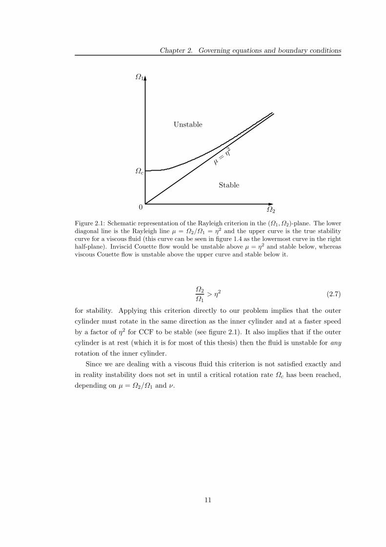
2.1 Schematic representation of the Rayleigh criterion in the (Ω1, Ω2)-plane.
The lower diagonal line is the Rayleigh line µ = Ω2/Ω1 = η2 and the
upper curve is the true stability curve for a viscous fluid (this curve can
be seen in figure 1.4 as the lowermost curve in the right half-plane).
Inviscid Couette flow would be unstable above µ = η2 and stable below,
whereas viscous Couette flow is unstable above the upper curve and
stable below it. . . . . . . . . . . . . . . . . . . . . . . . . . . . . . . . 11
iii
List of Figures
4.1 Steady Taylor–Couette flow. Critical wavenumber αc0 versus radius ratio
η. ( ) our results, ( ) Roberts’ (1965) results. . . . . . . . . 17
4.2 Steady Taylor–Couette flow. Critical Reynolds number Re0 versus ra-
dius ratio η. ( ) our results, ( ) Roberts’ (1965) results. . . 17
4.3 Radial velocity ur versus time in the middle of the gap at the outflow
computed at the (dimensionless) position z = π/α, r = (1 + η)/2(1 − η)
for reversing Taylor vortex flow. N = 16, K = 12, M = 1, η = 0.75,
Remod = 154.71 (which is Remod = 1.1Remod,c with Remod,c = 140.65),
ω = 3, αc = 2.86. Horizontal lines show ±Re0 = 85.78 and the dashed
curve is Re(t). . . . . . . . . . . . . . . . . . . . . . . . . . . . . . . . . 18
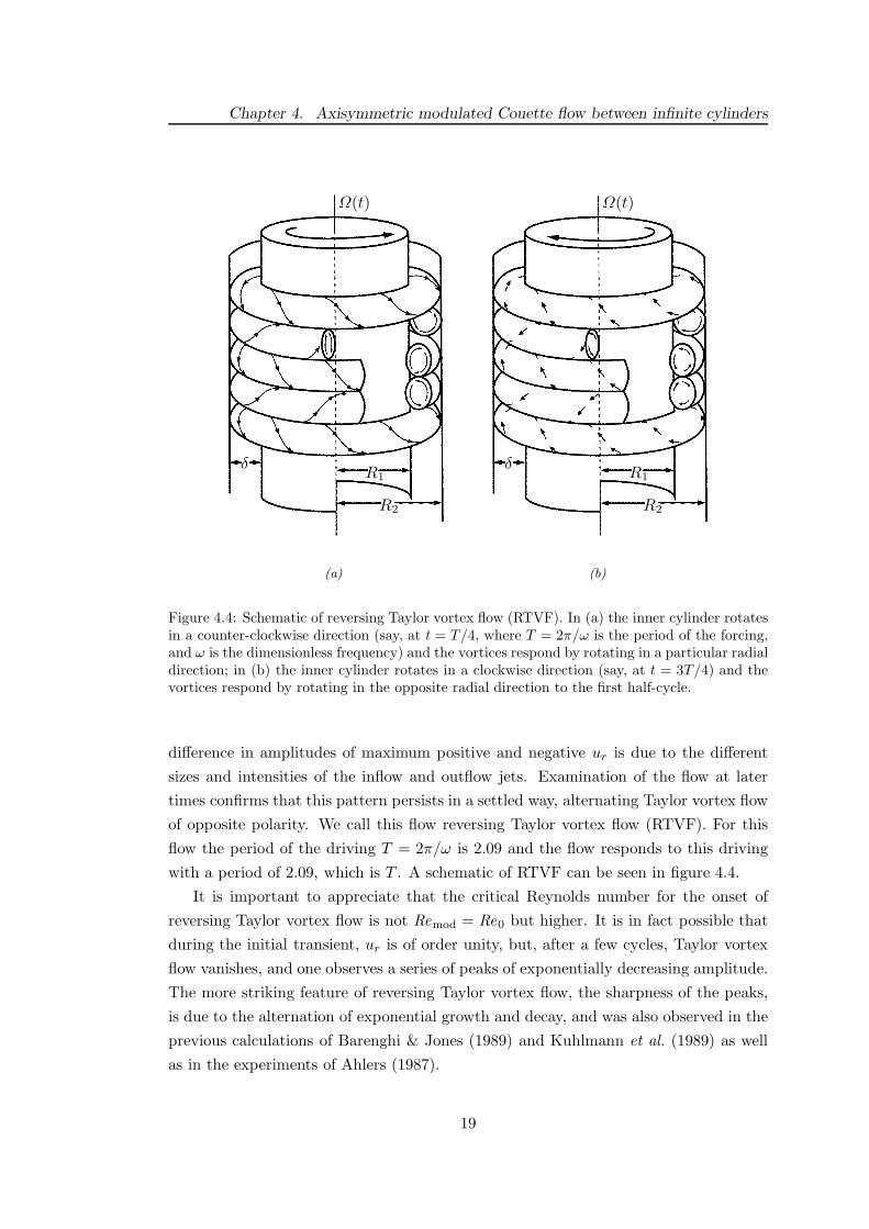
4.4 Schematic of reversing Taylor vortex flow (RTVF). In (a) the inner cylin-
der rotates in a counter-clockwise direction (say, at t = T/4, where
T = 2π/ω is the period of the forcing, and ω is the dimensionless fre-
quency) and the vortices respond by rotating in a particular radial di-
rection; in (b) the inner cylinder rotates in a clockwise direction (say, at
t = 3T/4) and the vortices respond by rotating in the opposite radial
direction to the first half-cycle. . . . . . . . . . . . . . . . . . . . . . . . 19
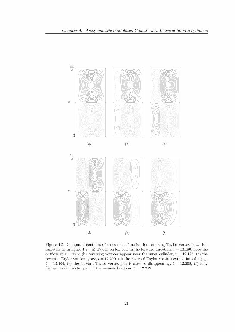
4.5 Computed contours of the stream function for reversing Taylor vortex
flow. Parameters as in figure 4.3. (a) Taylor vortex pair in the forward
direction, t = 12.180; note the outflow at z = π/α; (b) reversing vor-
tices appear near the inner cylinder, t = 12.196; (c) the reversed Taylor
vortices grow, t = 12.200; (d) the reversed Taylor vortices extend into
the gap, t = 12.204; (e) the forward Taylor vortex pair is close to dis-
appearing, t = 12.208; (f) fully formed Taylor vortex pair in the reverse
direction, t = 12.212. . . . . . . . . . . . . . . . . . . . . . . . . . . . . 21
4.6 Radial velocity ur versus time in the middle of the gap at the out-
flow computed again at the (dimensionless) position z = π/α, r =
(1 + η)/2(1 − η) for non-reversing Taylor vortex flow. Parameters as
in figure 4.3 except Remod = 170.41 (which is Remod = 1.1Remod,c with
Remod,c = 154.91), ω = 5, α = 3.73. Horizontal lines show ±Re0 = 85.78
and the dashed curve is Re(t). . . . . . . . . . . . . . . . . . . . . . . . 22
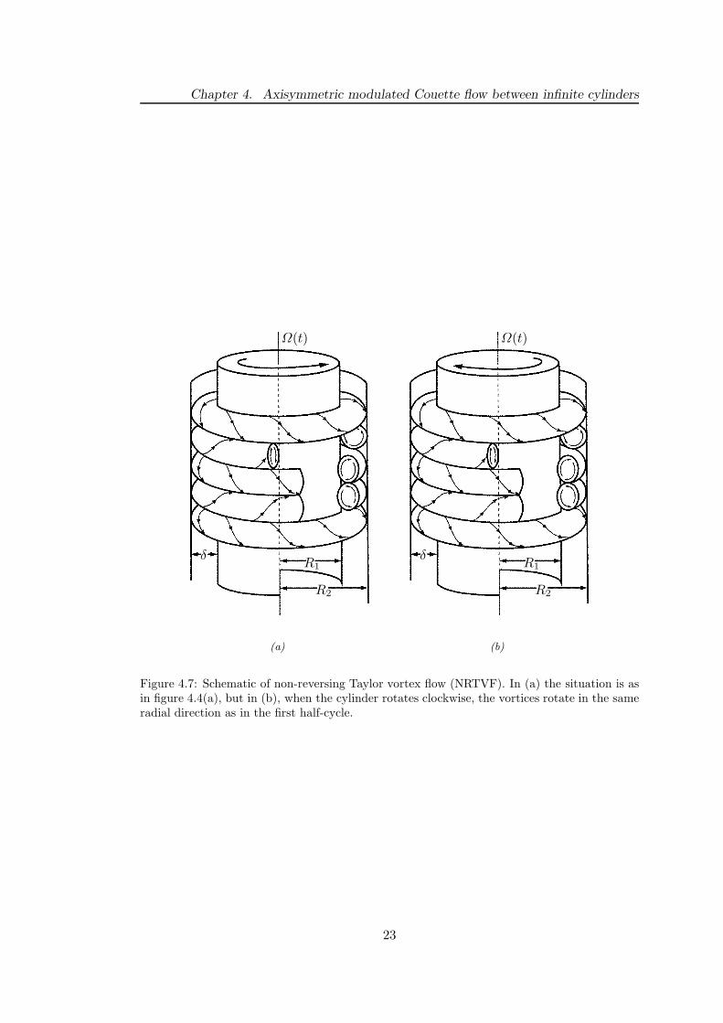
4.7 Schematic of non-reversing Taylor vortex flow (NRTVF). In (a) the situa-
tion is as in figure 4.4(a), but in (b), when the cylinder rotates clockwise,
the vortices rotate in the same radial direction as in the first half-cycle. 23
4.8 Critical wavenumber αc versus frequency of modulation ω for RTVF and
NRTVF at different radius ratios.
: η = 0.3, : η = 0.5, : η = 0.6,
: η = 0.7, : η = 0.75, : η = 0.8, and : η = 0.9. . . . . . . . . . 25
iv

List of Figures
4.9 Critical modulation amplitude Remod,c of the inner cylinder versus wavenum-
ber α for RTVF and NRTVF at three frequencies. . . . . . . . . . . . . 25
4.10 Critical Reynolds number Remod,c versus frequency ω for RTVF and
NRTVF at radius ratios η = 0.5–0.9.
: η = 0.5, : η = 0.6, :
η = 0.7,
: η = 0.75, : η = 0.8, : η = 0.9. Leftmost curves are
RTVF; rightmost curves are NRTVF. . . . . . . . . . . . . . . . . . . . 26
4.11 Critical frequency of intersection ω∗c of RTVF and NRTVF versus radius
ratio η. . . . . . . . . . . . . . . . . . . . . . . . . . . . . . . . . . . . . 27
4.12 Critical Reynolds number of intersection Re∗mod/Re0 versus radius ratio
η. . . . . . . . . . . . . . . . . . . . . . . . . . . . . . . . . . . . . . . . 28
4.13 Logarithm of the kinetic energy (in arbitrary units as in Willis & Barenghi,
2002a) of the first azimuthal modes m = 0 ( ), 1 ( ), 2
( ), and 3 ( ) versus time for RTVF. Parameters as in fig-
ure 4.3 but with M = 4. . . . . . . . . . . . . . . . . . . . . . . . . . . 30
4.14 Logarithm of the kinetic energy (in arbitrary units as in Willis & Barenghi,
2002a) of the first azimuthal modes m = 0 ( ), 1 ( ), 2
( ), and 3 ( ) versus time for NRTVF. Parameters as in
figure 4.6 but with M = 4. . . . . . . . . . . . . . . . . . . . . . . . . . 31
5.1 Contour plot of radial velocity ur for non-axisymmetric non-reversing
flow at a fixed azimuthal position. Choosing a different azimuthal posi-
tion has the effect of shifting the cells up or down slightly in the axial
direction. Note the trapezoidal deformation. Dashed lines represent
positive ur, solid lines represent negative ur. . . . . . . . . . . . . . . . 33
5.2 Radial velocity ur computed by tracking the Taylor vortex as explained
in the text, versus radial position r for non-axisymmetric reversing flow
(η = 0.8, ω = 4, Remod = 250). Each curve is plotted for a different
time with 195.704 6 t 6 195.749. The curves show ur < 0, initially,
and ur > 0 after the nodal line has crossed the gap. The filled circles
indicate the radial position where ur = 0. . . . . . . . . . . . . . . . . . 34
5.3 Contours of the radial velocity component for non-axisymmetric revers-
ing flow at one particular azimuthal position. (a) at t = 195.704, (b) at
t = 195.726, (c) at t = 195.749. Dashed lines represent positive ur, solid
lines represent negative ur. . . . . . . . . . . . . . . . . . . . . . . . . . 35
5.4 Radial velocity ur (measured at the dimensionless position z = π/α,
r = (1 + η)/2(1 − η)), versus t, for non-axisymmetric reversing flow
(η = 0.8, ω = 4, Remod = 250) over two forcing periods. Also shown is
the Reynolds number Re(t). The period of the forcing is 2π/4 ≈ 1.57
which the flow responds to synchronously. The time step is ∼ O(10−4). 36
v
List of Figures
5.5 Isosurfaces of helicity H = |u · (∇ ∧ u)| for non-axisymmetric reversing
flow with parameters as in figure 5.2 shown over two axial periods. The
predominant azimuthal mode is m = 1. The times of the plots are:
(a) t = 41.012, (b) t = 41.425, (c) t = 41.489, (d) t = 41.886. The
isosurface levels are taken at: (a) H ≈ 12, 000, (b) H ≈ 5, (c) H ≈ 30,
(d) H ≈ 6, 000. . . . . . . . . . . . . . . . . . . . . . . . . . . . . . . . . 37
5.6 Radial velocity ur versus radial position r for non-axisymmetric NRTVF
(η = 0.8, ω = 5, Remod = 400). Each curve is plotted for a different time
with 171.92 6 t 6 172.00. The curves show that ur < 0 for all times. . 38
5.7 Radial velocity ur (measured at the dimensionless position z = π/α,
r = (1 + η)/2(1 − η)), versus t, for non-axisymmetric non-reversing flow
(η = 0.8, ω = 5, Remod = 400) over two forcing periods. Also shown is
the Reynolds number Re(t). The period of the forcing is 2π/5 ≈ 1.26
which the flow responds to synchronously. The time step is ∼ O(6 ×
10−5). . . . . . . . . . . . . . . . . . . . . . . . . . . . . . . . . . . . . . 38
5.8 Isosurfaces of helicity H = |u · (∇ ∧ u)| for non-axisymmetric non-
reversing flow with parameters as in figure 5.6 shown over two axial
periods. The predominant azimuthal mode is m = 1. The times of
the plots are: (a) t = 171.738, (b) t = 171.936, (c) t = 171.955, (d)
t = 172.407. The isosurface levels are taken at: (a) H ≈ 18, 000, (b)
H ≈ 40, (c) H ≈ 5, (d) H ≈ 9, 000. . . . . . . . . . . . . . . . . . . . . 40
5.9 Logarithm of the kinetic energy of the m = 0 ( ) axisymmetric
mode and the m = 1 ( ), 2 ( ), and 3 ( ) azimuthal
modes versus time. . . . . . . . . . . . . . . . . . . . . . . . . . . . . . 41
6.1 Taylor–Couette flow at finite aspect ratio, η = 0.615. (a) 3-cell anoma-
lous mode with Γ = 3, Re = 240 and (b) 4-cell anomalous mode with
Γ = 4, Re = 240. . . . . . . . . . . . . . . . . . . . . . . . . . . . . . . 44
6.2 Stability curves for the 2- ( ), 3- ( ), and 4-cell ( )
anomalous modes at η = 0.615 for different values of the aspect ratio. . 48
6.3 Computed contours of the stream function of the (a) 1-cell and (b) 2-cell
flows at Γ = 1.2, η = 0.5, and Re = 400. . . . . . . . . . . . . . . . . . 49
6.4 Critical steady Reynolds number Rec versus aspect ratio Γ for the tran-
sition between 1- and 2-cell flows for η = 0.5. The arrows denote whether
the boundaries can be found by a quasi-static increase (↑) or decrease (↓)
of the Reynolds number. The inset is an enlargement of the hysteresis
region. . . . . . . . . . . . . . . . . . . . . . . . . . . . . . . . . . . . . 50
vi
List of Figures
6.5 Schematic bifurcation diagrams for the interaction between the 1- and
2-cell states after Pfister et al. (1988). The vertical axis shows the am-
plitude of the axial velocity uz in the middle of the gap at z = h/2 which
distinguishes between symmetric and asymmetric flows. The Reynolds
number is on the horizontal axis. Rec1 and Rec2 are the critical Reynolds
numbers for the onset of the 1-cell and 2-cell flows respectively. C1 de-
notes (stable) 1-cell branches; C2 denotes (stable) 2-cell branches. In (a)
the 1-cell solution branch is connected (the curve AB in figure 6.4); in (b)
there is hysteresis between the 1- and 2-cell flows (BC); in (c) the 1-cell
solution branch is disconnected (BE). Stable branches are shown as solid
lines; unstable branches as dashed lines. . . . . . . . . . . . . . . . . . . 51
8.1 Maximum positive amplitude (solid) and maximum negative amplitude
(dashed) of the radial velocity ur (at the midpoint r = 1 + η/2(1 − η)
and z = Γ/2) versus amplitude of modulation Remod for NRTVF at
η = 0.75, Γ = 8, and ω = 3. . . . . . . . . . . . . . . . . . . . . . . . . 60
8.2 Radial velocity ur (at the midpoint r = 1 + η/2(1 − η) and z = Γ/2)
versus time over a cycle for NRTVF at η = 0.75, Γ = 8, ω = 3, and
Remod = 140 (solid). Also shown (dashed) is the Reynolds number
Re(t) — see vertical axis on the right. In this and subsequent time-
series figures, we plot the achieved settled oscillations past the initial
transient; t is the time taken from the initial time t = 0. . . . . . . . . 61
8.3 Computed contour plots of the stream function over the whole length of
the cylinder 0 6 z 6 8 showing the problems presented by the choice
of contour levels. In (a) the number of contour levels is chosen so as to
capture the structure at the ends, but this hides the structure close to
the midplane; in (b) the number of contour levels is chosen so as to show
the structure at the midplane, but now the contours are too dense close
to the ends. . . . . . . . . . . . . . . . . . . . . . . . . . . . . . . . . . 62
8.4 Computed contours of the stream function for a non-reversing flow at
Γ = 8, η = 0.75, ω = 3, Remod = 140, plotted only for 1 6 z 6 7.
When the vortices form there are Γ = 8 cells within the gap. The flow
responds to the driving (period T = 2π/ω) with period T/2. The times
of the snapshots are (a) t = 4.246 (which corresponds to 0.308T during
a cycle which begins at t = 3.600), (b) t = 4.318 (0.343T ), (c) t = 4.495
(0.427T ), (d) t = 4.856 (0.600T ), (e) t = 4.887 (0.614T ), (f) t = 4.939
(0.639T ). . . . . . . . . . . . . . . . . . . . . . . . . . . . . . . . . . . . 63
8.5 Radial velocity ur versus time over a cycle as in figure 8.2 for NRTVF
with the same parameters except Remod = 155. . . . . . . . . . . . . . 64
vii

List of Figures
8.6 Computed contours of the stream function for a non-reversing flow at
Γ = 8, η = 0.75, ω = 3, Remod = 155, and for 1 6 Γ 6 7. When the
vortices form there are Γ = 8 cells within the gap. The flow responds
to the driving with period T/2. The times of the snapshots are (a)
t = 5.254 (which corresponds to 0.312T during a cycle which begins at
t = 4.600), (b) t = 5.410 (0.387T ), (c) t = 5.629 (0.491T ), (d) t = 5.906
(0.624T ), (e) t = 5.938 (0.639T ), (f) t = 6.042 (0.689T ). . . . . . . . . . 66
8.7 Radial velocity ur versus time over a cycle as in figure 8.2 for NRTVF
with the same parameters except Remod = 180. . . . . . . . . . . . . . 67
8.8 Computed contours of the stream function for a non-reversing flow at
Γ = 8, η = 0.75, ω = 3, Remod = 180, and for 1 6 Γ 6 7. When
the vortices form there are Γ + 2 = 10 cells within the gap. The flow
responds to the driving with period T/2. The times of the snapshots
are (a) t = 4.156 (which corresponds to 0.256T during a cycle which
begins at t = 3.620), (b) t = 4.198 (0.276T ), (c) t = 4.281 (0.316T ), (d)
t = 4.777 (0.552T ), (e) t = 4.870 (0.597T ), (f) t = 4.933 (0.627T ). . . . 68
8.9 Maximum positive amplitude (solid) and maximum negative amplitude
(dashed) of the radial velocity ur (measured at r = 1 + η/2(1 − η) and
z = Γ/2) versus amplitude of modulation Remod for RTVF at η = 0.75,
Γ = 14, and ω = 3. . . . . . . . . . . . . . . . . . . . . . . . . . . . . . 69
8.10 Radial velocity ur versus time over a cycle as in figure 8.2 for RTVF
with the same parameters except Γ = 14 and Remod = 170. The flow
responds synchronously to the driving with a period of T . . . . . . . . 70
8.11 Computed contours of the stream function for a reversing flow at Γ = 14,
η = 0.75, ω = 3, Remod = 170, plotted in the region 0 6 z 6 7 only.
When the vortices form there are (a) Γ = 14 cells within the gap in the
first part of the cycle and (b) Γ + 2 = 16 cells in the second part of the
cycle. The flow responds to the driving with period T . . . . . . . . . . 71
8.12 Computed contours of the stream function for a reversing flow at Γ = 14,
η = 0.75, ω = 3, Remod = 170, plotted in 3 6 z 6 11 only as the reversal
process takes place. The flow responds to the driving with period T . The
times of the snapshots are (a) t = 6.916 (which corresponds to 0.581T
during a cycle which begins at t = 5.700), (b) t = 6.956 (0.600T ), (c)
t = 6.962 (0.603T ), (d) t = 6.966 (0.604T ), (e) t = 6.970 (0.606T ), (f)
t = 7.006 (0.624T ). Note how the B cells are pushed radially out until
they disappear. . . . . . . . . . . . . . . . . . . . . . . . . . . . . . . . 73
viii
List of Figures
8.13 Computed contours of the stream function showing the appearance of
extra cells in the second part of the cycle of a reversing flow with non-
even aspect ratio Γ = 15, Remod = 150, and ω = 3. The appearance of
the extra cells means that 18 cells try to fit in the gap, but the aspect
ratio is not large enough and they are squeezed out leaving 14 cells. The
flow responds to the driving with period T . The times of the snapshots
are (a) t = 12.812 (which corresponds to 0.497T during a cycle which
begins at t = 11.771), (b) t = 12.874 (0.527T ), (c) t = 12.979 (0.577T ),
(d) t = 13.000 (0.587T ), (d) t = 13.104 (0.636T ), (f) t = 13.209 (0.687T ). 75
8.14 Computed contours of the stream function for the oscillation between
1- and 2-cell flows at Γ = 1, η = 0.5, ω = 4, Remod = 400. The
times of the snapshots are (a) t = 17.059 (which corresponds to 0.006T
during a cycle which begins at t = 17.050), (b) t = 17.355 (0.194T ), (c)
t = 17.433 (0.244T ), (d) t = 17.612 (0.358T ), (e) t = 17.729 (0.432T ),
(f) t = 17.807 (0.482T ). . . . . . . . . . . . . . . . . . . . . . . . . . . . 77
8.15 Computed contours of the stream function for the oscillating ‘side-by-
side’ flow at Γ = 0.7, η = 0.5, ω = 3, Remod = 1500. The times of
the snapshots are (a) t = 12.177 (which corresponds to 0.207T during a
cycle which begins at t = 11.743), (b) t = 12.239 (0.237T ), (c) t = 12.721
(0.467T ), (d) t = 13.025 (0.612T ), (e) t = 13.088 (0.642T ), (f) t = 13.161
(0.677T ). . . . . . . . . . . . . . . . . . . . . . . . . . . . . . . . . . . . 79
10.1 Critical Reynolds number Rec versus aspect ratio Γ for the transition
between the 1- and 2-cell flows (as figure 6.4) in the presence of various
applied magnetic fields Q. Q = 0 ( ), Q = 5 ( ), Q = 10
( ), Q = 50 ( ), Q = 100 ( ). . . . . . . . . . . . . . . 89
10.2 Critical aspect ratio Γc versus Q (the point at which the 1-cell flow is no
longer realisable by a quasi-static increase of Re across the curve AB or
decrease across the curve CD). . . . . . . . . . . . . . . . . . . . . . . . 90
10.3 Computed contours of various fields for a 2-cell flow for Q = 100, Re =
500, Γ = 0.97. (a) radial velocity ur, (b) azimuthal velocity uθ (including
the underlying circular Couette flow), (c) axial velocity uz, (d) stream
function ψ, (e) azimuthal magnetic field Bθ, (f) azimuthal current Jθ. . 91
10.4 Contour plots as in figure 10.3 with the same parameters but now for a
1-cell flow. . . . . . . . . . . . . . . . . . . . . . . . . . . . . . . . . . . 92
ix
List of Figures
10.5 Critical Reynolds number Retd versus aspect ratio Γ for the transition to
time-dependent motion at various strengths of magnetic field Q. To the
left of the vertical bar on each curve (which corresponds to the aspect
ratio of the point C) the time-dependent boundary can be realised by a
quasi-static increase or decrease of the Reynolds number; to the right it
can only be found by a quasi-static decrease. . . . . . . . . . . . . . . . 93
10.6 Schematic bifurcation diagrams (a) to the left and (b) to the right of
the intersection point of curves CD and XY. The arrows denote the
critical Reynolds number at which the 2-cell flow loses stability to (a)
the time-dependent flow and (b) the 1-cell flow. . . . . . . . . . . . . . 94
10.7 Frequency f of the oscillations at the onset of axisymmetric time-dependence
versus aspect ratio Γ at various strengths of magnetic field Q. f is non-
dimensionalised with respect to the inner cylinder angular frequency
Ω. The relation between f and ω, the frequency which has been non-
dimensionalised with respect to the diffusion time δ2/ν is ω = Re(1 −
η)f/η. . . . . . . . . . . . . . . . . . . . . . . . . . . . . . . . . . . . . 95
10.8 Snapshots of the stream function over one period for the time-dependent
flow for Q = 10, Re = 400, and Γ = 1.7. (a) t = 25.9857, (b) t =
25.9962, (c) t = 25.9998, (d) t = 26.0034, (e) t = 26.0091, (f) t =
26.0142. . . . . . . . . . . . . . . . . . . . . . . . . . . . . . . . . . . . 96
10.9 Snapshots of the stream function over one period for the time-dependent
2-cell flow for Q = 10, Re = 700, and Γ = 1.3. (a) t = 4.0453, (b)
t = 4.0477, (c) t = 4.0500, (d) t = 4.0524, (e) t = 4.0548, (f) t = 4.0572. 97
10.10Reynolds number versus aspect ratio highlighting the boundary (ST) for
the transition to the 2-cell time-dependent flow, for Q = 0. . . . . . . . 98
10.11Reynolds number versus aspect ratio as in figure 10.10 but now for Q =
10. . . . . . . . . . . . . . . . . . . . . . . . . . . . . . . . . . . . . . . 98
x
List of Tables
3.1 Error in the linear growth rates σ as the truncation N → ∞ compared to
the value of σ = 0.430108693 obtained by Barenghi (1991). η = 1/1.444,
α = 3.13, Re = 80. . . . . . . . . . . . . . . . . . . . . . . . . . . . . . . 14
3.2 Radial velocity at the outflow jet at r = (R1 + R2)/2, z = π/α at
three different Reynolds numbers for the time step ∆t → 0. η = 0.5,
α = 3.1631. The values found by Jones (1985a) at the three Reynolds
numbers are 4.23363, 17.9705, and 33.6805. . . . . . . . . . . . . . . . . 14
3.3 Wavespeeds of the (m = 6) azimuthal waves in non-axisymmetric wavy
vortex flow as a fraction of the rotation rate of the inner cylinder for
η = 0.868, Re0 = 115.1. . . . . . . . . . . . . . . . . . . . . . . . . . . . 15
7.1 Growth rates σ and percentage errors at various mesh sizes and time
steps. The number of axial grid points is twice the number of radial
grid points Nr. The radius ratio is η = 1/1.444, the axial wavenumber
α = 3.13, the Reynolds number is Re = 80, and the growth rate as
calculated by Barenghi (1991) using a spectral code is σ = 0.430108693. 55
7.2 Radial velocity at the outflow jet r = (R1 +R2)/2, z = π/α and percent-
age errors at three different Reynolds numbers for different time steps
and spatial resolutions Nr compared to the values obtained by Jones
(1985a) (4.23363, 17.9705, and 33.6805). . . . . . . . . . . . . . . . . . 56
9.1 Comparison of our results (under the small Prandtl number limit) and
those of Rudiger & Shalybkov (2002) (for Pm = 10−5) for critical wavenum-
bers and Reynolds numbers at the onset of Taylor vortex flow in the
presence of various strengths of applied axial magnetic field at η = 0.25.
Nr = 40 radial grid points, Nz = 2Nr axial grid points and the time
step is ∆t = 10−4. In their paper they state the magnetic field strength
in terms of the Hartmann number Ha and the relation to Q is Ha2 =
ηQ/(1 − η). They also state a different form of wavenumber k and the
relation to our α is α = k√
(1 − η)/η. . . . . . . . . . . . . . . . . . . . 85
xi

List of Tables
9.2 Comparison of our results and those of Chen & Chang (1998) and Chan-
drasekhar (1961) for critical wavenumbers and Reynolds numbers at the
onset of Taylor vortex flow in the presence of various strengths of applied
axial magnetic field at η = 0.95 but now allowing for counter-rotation
of the cylinders. Mesh sizes and time steps as in table 9.1. The critical
Reynolds numbers of Chandrasekhar and Chen & Chang were originally
stated in terms of the Taylor number Ta. The relation to our Reynolds
number is Re =√
ηTa/4(1 − η). . . . . . . . . . . . . . . . . . . . . . . 85
C.1 Steady critical wavenumbers αc0 and Reynolds numbers Re0 of our code
and those of Roberts (1965) for the onset of Taylor vortex flow at various
radius ratios η. . . . . . . . . . . . . . . . . . . . . . . . . . . . . . . . . 109
C.2 Critical wavenumbers αc and critical modulation amplitudes Remod,c for
the onset of RTVF and NRTVF at various frequencies ω. . . . . . . . . 110
C.3 Critical Reynolds numbers at various aspect ratios for the interaction
between the 1- and 2-cell flows in the absence of a magnetic field (Q = 0).
The labels AB, CD, and BE denote the parts of the curves shown in
figure 6.4. The points close to the hysteresis region are found to a higher
degree of accuracy. . . . . . . . . . . . . . . . . . . . . . . . . . . . . . 111
xii
Chapter 1
Introduction
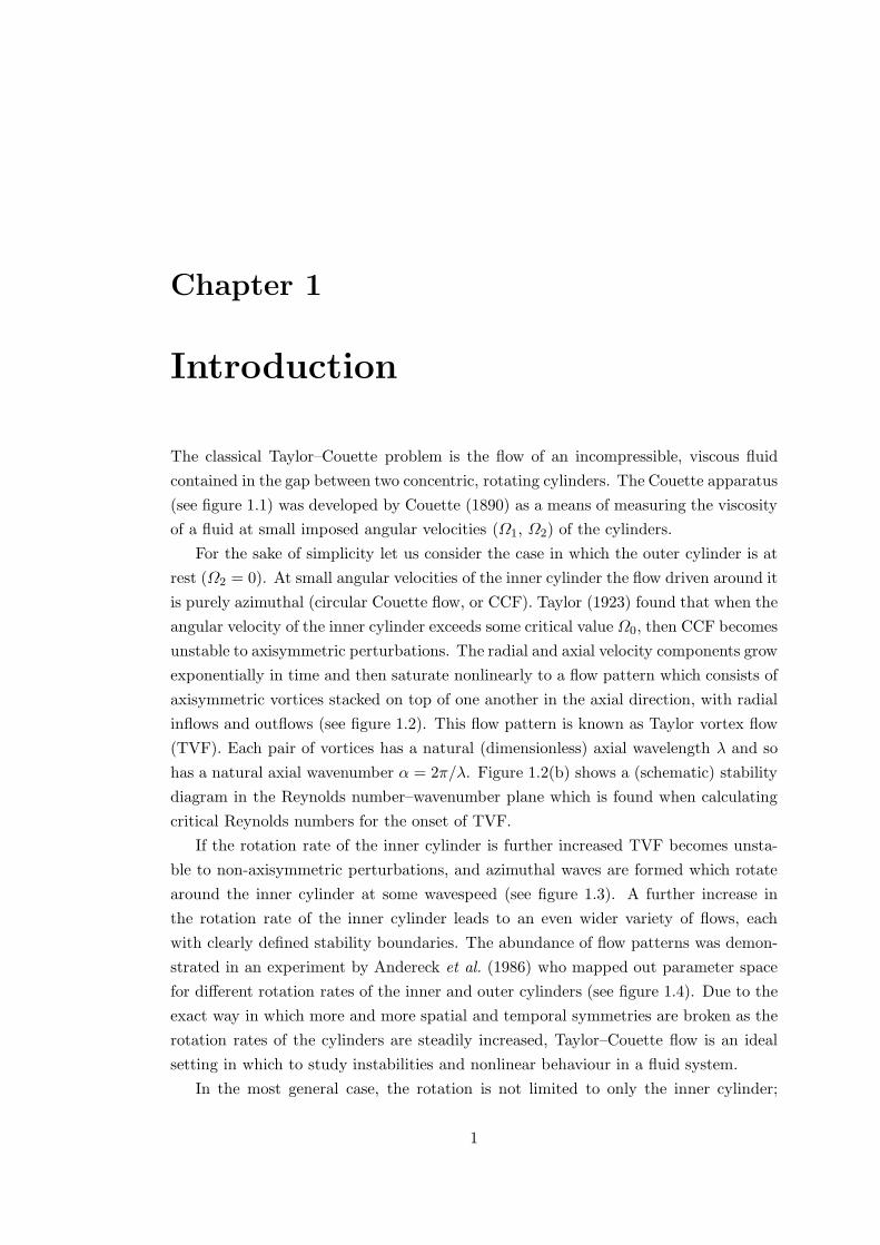
The classical Taylor–Couette problem is the flow of an incompressible, viscous fluid
contained in the gap between two concentric, rotating cylinders. The Couette apparatus
(see figure 1.1) was developed by Couette (1890) as a means of measuring the viscosity
of a fluid at small imposed angular velocities (Ω1, Ω2) of the cylinders.
For the sake of simplicity let us consider the case in which the outer cylinder is at
rest (Ω2 = 0). At small angular velocities of the inner cylinder the flow driven around it
is purely azimuthal (circular Couette flow, or CCF). Taylor (1923) found that when the
angular velocity of the inner cylinder exceeds some critical value Ω0, then CCF becomes
unstable to axisymmetric perturbations. The radial and axial velocity components grow
exponentially in time and then saturate nonlinearly to a flow pattern which consists of
axisymmetric vortices stacked on top of one another in the axial direction, with radial
inflows and outflows (see figure 1.2). This flow pattern is known as Taylor vortex flow
(TVF). Each pair of vortices has a natural (dimensionless) axial wavelength λ and so
has a natural axial wavenumber α = 2π/λ. Figure 1.2(b) shows a (schematic) stability
diagram in the Reynolds number–wavenumber plane which is found when calculating
critical Reynolds numbers for the onset of TVF.
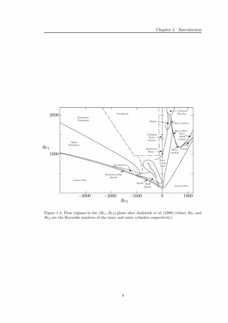
If the rotation rate of the inner cylinder is further increased TVF becomes unsta-
ble to non-axisymmetric perturbations, and azimuthal waves are formed which rotate
around the inner cylinder at some wavespeed (see figure 1.3). A further increase in
the rotation rate of the inner cylinder leads to an even wider variety of flows, each
with clearly defined stability boundaries. The abundance of flow patterns was demon-
strated in an experiment by Andereck et al. (1986) who mapped out parameter space
for different rotation rates of the inner and outer cylinders (see figure 1.4). Due to the
exact way in which more and more spatial and temporal symmetries are broken as the
rotation rates of the cylinders are steadily increased, Taylor–Couette flow is an ideal
setting in which to study instabilities and nonlinear behaviour in a fluid system.
In the most general case, the rotation is not limited to only the inner cylinder;
1
Chapter 1. Introduction
h δ
R1 R2
Ω1 Ω2
Figure 1.1: Schematic of the Couette apparatus. In general, Ω1 and Ω2 can independently bepositive, negative or zero. The height of the cylinders h is often taken to be very large (or eveninfinite) to minimise end effects. The infinite cylinder approximation does not, however, allowfor the existence of some interesting solutions.
2

Chapter 1. Introduction
Ω1
δ
R2
R1
(a)
Stable
Stable
Unstable
Re
Rec
ααc
(b)
Figure 1.2: Schematic of Taylor vortex flow (TVF). (a) When circular Couette flow becomesunstable, axisymmetric vortices form, which are stacked on top of each other in the axialdirection. The resulting velocity has an azimuthal component on top of the existing CCFvelocity component, and radial and axial components which produce a rotational motion in the(r, z)-plane. (b) Stability diagram for the onset of TVF. Couette flow is stable in the unshadedregion of the (Re, α)-plane (where Re is a measure of the rotation rate of the inner cylinder) andunstable to axisymmetric perturbations in the shaded region. The critical Reynolds numberand wavenumber for the onset of TVF is given by the minimum of this curve.
δ
Ω1
R2
R1
Figure 1.3: Schematic of Wavy vortex flow (WVF) — a secondary transition above TVF.The Taylor vortices become unstable to non-axisymmetric perturbations and rotate with somewavespeed around the axis of rotation.
3
Chapter 1. Introduction
Couette Flow
Couette Flow
Unexplored
FeaturelessTurbulence
TurbulenceSpiral
Interpenetrating
Intermittency
Wavelets
FlowVortex
Ripple
ModulatedWaves
Wavy
Wavy
Wavy
WavyInflow
+Twists
Wavy Inflow
Wavy Vortices
Corkscrew
Spirals
Spirals
Spirals
TurbulentTaylor
Vortices
Modulated
Waves
Twists
Outflow1000
2000
Re1
Re2
10000−1000−2000−3000
Figure 1.4: Flow regimes in the (Re1,Re2)-plane after Andereck et al. (1986) (where Re1 andRe2 are the Reynolds numbers of the inner and outer cylinders respectively).
4
Chapter 1. Introduction
many experiments and calculations have been performed where both cylinders rotate,
and in the counter-rotating case it is possible for non-axisymmetric perturbations to
go unstable first.
Much computational and theoretical work on Taylor–Couette flow assumes that the
cylinders are very long; more precisely, that the ratio of the height of the cylinders to
the gap width is large. In this case, effects due to the presence of the ends can be
ignored and the flow pattern has a natural axial wavenumber. It has long been noted,
however, that the ends of the top and bottom of the cylinders do have significant effects
on the flow, especially when the cylinders are short, and this problem was addressed in
detail by Benjamin (1978a,b). Indeed, Benjamin & Mullin (1981) found flow structures
(termed the ‘anomalous’ modes) that only exist when end effects are taken into account.
See chapter 6 for a detailed description of these solutions.
Plan of the thesis
For much of this work we shall be concerned with the case in which the outer cylinder
is held fixed Ω2 = 0 and Ω1 is not constant but oscillates harmonically in time. (To
simplify notation we shall generally drop the subscript 1 when it is clear that we are
only talking about inner cylinder rotation; if both cylinders are rotating the subscript
will be reinstated.) This modulated Taylor–Couette problem has been the subject of a
number of investigations which attempted to answer the natural question as to whether
the modulation makes the flow more or less stable to the onset of vortices than in the
steady case. The problem can also be tackled in the context of spherical Couette flow,
as recently done by Zhang (2002). The oscillating boundary induces a damped viscous
wave which penetrates into the fluid a distance of the order of the thickness of the
Stokes layer δs = (2ν/ω)1/2 where ν is the kinematic viscosity and ω is the frequency of
modulation. See appendix A for a detailed calculation of the form of the viscous wave.
In this thesis we are concerned with the basic case in which the frequency is low enough
so that the size of the Stokes layer is comparable to the gap between the cylinders. The
high frequency limit of a thin Stokes layer, which was studied for example by Barenghi
et al. (1980) in cylindrical geometry and by Hollerbach et al. (2002) in spherical Couette
flow, will not be addressed here.
The most studied case of modulated Couette flow is that in which the angular
velocity of the inner cylinder oscillates about some mean value Ωm with some given
amplitude Ωa
Ω(t) = Ωm +Ωa cos (ωt), (1.1)
such that the peak angular velocity Ωm +Ωa is of the order of the onset of vortices in
the steady case Ω0. In particular, we note the experiments of Donnelly (1964), Walsh
5
Chapter 1. Introduction
et al. (1987), and Walsh & Donnelly (1988), who discovered that at low frequency of
modulation the stability of the flow is greatly enhanced. On the theoretical side, the
problem was tackled in the narrow gap limit by Hall (1983), who derived an amplitude
equation, and by Riley & Laurence (1976, 1977), who used Floquet theory. Carmi &
Tustaniwskyj (1981) extended the Floquet approach to finite values of radius ratio.
Barenghi & Jones (1989) and Barenghi (1991) solved the Floquet problem as well as
the fully nonlinear time-dependent Navier–Stokes equation, and compared their finite-
amplitude, time-dependent solutions against measurements. A similar approach was
followed by Kuhlmann et al. (1989), who also developed a mode truncation model.
Mode truncation was also used by Hsieh & Chen (1984) and Bhattacharjee et al.
(1986). Almost all these authors did not limit themselves to the most studied case
(equation (1.1) with Ωm + Ωa ≈ Ω0), but studied other variations of the problem,
including steady and periodic motions of the outer cylinder. More recently a new
class of time modulated Taylor–Couette problems in which the inner cylinder moves
periodically in the axial direction has been introduced and studied by Marques & Lopez
(1997) and Lopez & Marques (2001).
In chapter 2 we set up the governing equations and boundary conditions and chap-
ter 3 details a numerical formulation suitable for studying modulated flows under the
infinite cylinder approximation. In chapter 4 we look at a simple variation of the mod-
ulated problem where the outer cylinder is held fixed and the inner cylinder oscillates
around zero mean
Ω(t) = Ωa cos (ωt). (1.2)
We begin by presenting a new class of solutions in this regime. Initially, the results are
all axisymmetric. Chapter 5 focuses on non-axisymmetric results in the same setting.
The next chapters are concerned with the more realistic setting of finite length
cylinders. Chapter 6 gives a brief outline of flow solutions which do not exist under
the infinite cylinder approximation — the so-called ‘anomalous’ modes. Chapter 7
describes a new numerical formulation which allows for the existence of end-plates
which are attached to the (fixed) outer cylinder.
The goal of chapter 8 is to extend the axisymmetric results of chapter 4 to the case
where the cylinders have finite height. We attempt to answer the question whether the
presence of the ends suppresses the results found assuming infinite height cylinders.
We also explore an extreme example of finite height cylinders where the height of the
cylinders is on the order of the gap between them. In this regime we want to examine
the effect of a modulation on the 1- and 2-cell flow patterns that exist here.
For the second part of the thesis we turn our attention away from modulation of the
inner cylinder to look at the effect of a body force on the existence of the 1- and 2-cell
6

Chapter 1. Introduction
flows that exist when the cylinders are very short. An applied axial magnetic field will
provide the body force, and so in chapter 9 we set up the hydromagnetic equations,
before describing the results in this regime in chapter 10. Finally, chapter 11 draws
some conclusions and points to future work.
The material in chapters 4 and 5 is published in Youd et al. (2003) and Youd et al.
(2005). The material in chapter 10 will be published in Youd & Barenghi (2005a) and
the material in chapter 8 will be published in Youd & Barenghi (2005b).
7
Part I
Hydrodynamic
8
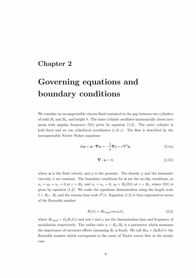
Chapter 2
Governing equations and
boundary conditions
We consider an incompressible viscous fluid contained in the gap between two cylinders
of radii R1 and R2, and height h. The inner cylinder oscillates harmonically about zero
mean with angular frequency Ω(t) given by equation (1.2). The outer cylinder is
held fixed and we use cylindrical coordinates (r, θ, z). The flow is described by the
incompressible Navier–Stokes equations
∂tu + u · ∇u = −1
ρ∇p+ ν∇2
u, (2.1a)
∇ · u = 0, (2.1b)
where u is the fluid velocity and p is the pressure. The density ρ and the kinematic
viscosity ν are constant. The boundary conditions for u are the no-slip conditions, so
ur = uθ = uz = 0 at r = R2, and ur = uz = 0, uθ = R1Ω(t) at r = R1, where Ω(t) is
given by equation (1.2). We make the equations dimensionless using the length scale
δ = R2−R1 and the viscous time scale δ2/ν. Equation (1.2) is then expressed in terms
of the Reynolds number
Re(t) = Remod cos (ωt), (2.2)
where Remod = ΩaR1δ/ν and now t and ω are the dimensionless time and frequency of
modulation respectively. The radius ratio η = R1/R2 is a parameter which measures
the importance of curvature effects (assuming R1 is fixed). We call Re0 = Ω0R1δ/ν the
Reynolds number which corresponds to the onset of Taylor vortex flow in the steady
case.
9
Chapter 2. Governing equations and boundary conditions
Another parameter in the problem is the aspect ratio Γ = h/δ (the ratio of the
height of the cylinders to the gap between them). Initial calculations will assume that
h δ and so we shall assume the infinite cylinder approximation Γ → ∞ where we
ignore end effects. We shall examine the more realistic setting of Γ < ∞ (i.e. finite
height cylinders) in later chapters.
In the steady case, when the inner cylinder rotation does not depend on time, CCF
(u = uθ(r)θ) is a solution of the Navier–Stokes equations. It takes the form
uθ(r) = Ar +B
r, (2.3)
where A and B are constants which (in general) depend on the angular frequencies and
radii of both cylinders.
In the most general case where both the inner and outer cylinders are allowed to
rotate, CCF has the dimensionless form
uθ(r) =Re2 − ηRe1
1 + ηr +
η (Re1 − ηRe2)
(1 + η)(1 − η)21
r, (2.4)
where Re i = ΩiRiδ/ν is the steady Reynolds number of the inner (i = 1) and outer
(i = 2) cylinder.
In the modulated case the basic state is no longer circular Couette flow; instead the
solution takes the form of a viscous wave which penetrates into the gap a distance of
the Stokes layer δs = (2ν/ω)1/2. Appendix A gives details as to the exact form of this
solution.
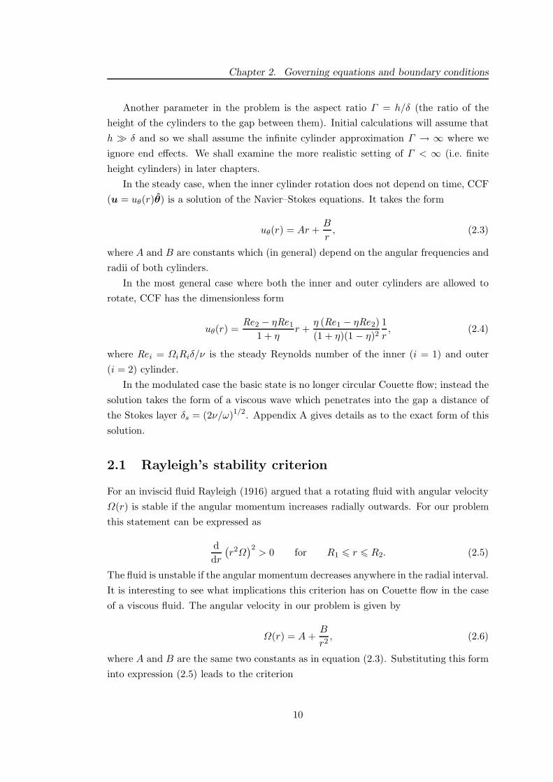
2.1 Rayleigh’s stability criterion
For an inviscid fluid Rayleigh (1916) argued that a rotating fluid with angular velocity
Ω(r) is stable if the angular momentum increases radially outwards. For our problem
this statement can be expressed as
d
dr
(
r2Ω)2> 0 for R1 6 r 6 R2. (2.5)
The fluid is unstable if the angular momentum decreases anywhere in the radial interval.
It is interesting to see what implications this criterion has on Couette flow in the case
of a viscous fluid. The angular velocity in our problem is given by
Ω(r) = A+B
r2, (2.6)
where A and B are the same two constants as in equation (2.3). Substituting this form
into expression (2.5) leads to the criterion
10
Chapter 2. Governing equations and boundary conditions
0
Ω1
Ωc
Ω2
Stable
Unstable
µ=η2
Figure 2.1: Schematic representation of the Rayleigh criterion in the (Ω1, Ω2)-plane. The lowerdiagonal line is the Rayleigh line µ = Ω2/Ω1 = η2 and the upper curve is the true stabilitycurve for a viscous fluid (this curve can be seen in figure 1.4 as the lowermost curve in the righthalf-plane). Inviscid Couette flow would be unstable above µ = η2 and stable below, whereasviscous Couette flow is unstable above the upper curve and stable below it.
Ω2
Ω1> η2 (2.7)
for stability. Applying this criterion directly to our problem implies that the outer
cylinder must rotate in the same direction as the inner cylinder and at a faster speed
by a factor of η2 for CCF to be stable (see figure 2.1). It also implies that if the outer
cylinder is at rest (which it is for most of this thesis) then the fluid is unstable for any
rotation of the inner cylinder.
Since we are dealing with a viscous fluid this criterion is not satisfied exactly and
in reality instability does not set in until a critical rotation rate Ωc has been reached,
depending on µ = Ω2/Ω1 and ν.
11
Chapter 3
Numerical formulation I
Full details of the numerical method used for the first part of this thesis can be found
in Willis & Barenghi (2002a). In this chapter we provide an outline of the numerical
code which allows for fully non-axisymmetric simulations under the infinite cylinder
approximation. The code also allows for the application of an axial magnetic field; in
this thesis, however, we do not study hydromagnetic Couette flow under the infinite
cylinder approximation, and so we do not describe the magnetic parts of the code.
We first rewrite (the dimensionless form of) equations (2.1) with u = u + u′ and
p = p+ p′ where u is the underlying circular Couette flow, p is the basic pressure, and
u′ and p′ are perturbations. u′ then satisfies the Dirichlet boundary condition u′ = 0
at r = R1 and R2. The dimensionless equations for u′ are
(
∂t −∇2)
u′ = N − ∇p′, (3.1a)
∇ · u′ = 0, (3.1b)
where the nonlinear term is N = (u · ∇) u′ + (u′· ∇) u. Hence, the calculations are
fully nonlinear and linear growth rates are obtained by using a small initial seed on the
order of 10−10.
The code uses a primitive variable, toroidal–poloidal potential formulation in which
variables are expanded in the form
A = ψ0θ + φ0z + ∇ ∧ (ψr) + ∇ ∧ ∇ ∧ (φr) . (3.2)
ψ(r, t, z) and φ(r, t, z) contain the periodic parts of the solution and ψ0(r) and φ0(r)
contain the non-periodic parts. r is the cylindrical-polar radius.
The expansion (3.2) for the velocity field is substituted into equation (3.1a) and
12

Chapter 3. Numerical formulation I
then the non-periodic part satisfies
∂t −
(
∇2 −1
r2
)
ψ0 = θ · N , (3.3a)
(
∂t −∇2)
φ0 = z · N , (3.3b)
with ψ0 = φ0 = 0 at r = R1 and R2.
For the periodic part the first curl of the momentum equation is used and since
the pressure has not been eliminated we also take the divergence. The equations are
(dropping all primes)
2
r2∂θzψ −∇2
c
(
∂t − ∇2)
φ−2
r3∂rθθφ =
1
r2r · (N − ∇p) , (3.4a)
−∇2c
(
∂t − ∇2)
ψ −2
r3∂rθθψ +
2
r2(
∂t − 2∇2)
∂θzφ =1
r2r · ∇ ∧ N , (3.4b)
∇2p = ∇ · N , (3.4c)
where ∇2 = ∇2 + (2/r) ∂r and ∇2c = 1/r2 + ∂zz.
The boundary conditions uθ = uz = 0 at the walls lead to
r∂zψ + ∂rθφ = 0, (3.5a)
−∂θψ + (2 + r∂r) ∂zφ = 0, (3.5b)
and the Poisson equation for the pressure is solved using the boundary condition ur = 0,
which leads to
∇2cφ = 0. (3.6)
Equations (3.4) are time stepped using a combination of the second order accurate
implicit Crank–Nicolson scheme for the linear terms and the explicit Adams–Bashforth
scheme for the nonlinear terms. The velocity components are expanded spectrally over
Fourier modes in the azimuthal and axial directions and over Chebyshev polynomials
in the radial direction, for which a generic field A(x, θ, z, t) has the form
13
Chapter 3. Numerical formulation I
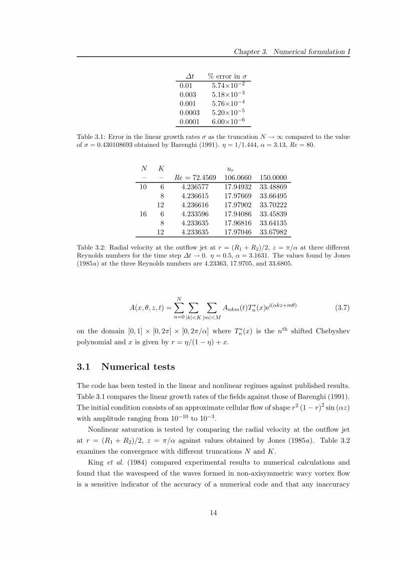
∆t % error in σ
0.01 5.74×10⁻²
0.003 5.18×10⁻³
0.001 5.76×10⁻⁴
0.0003 5.20×10⁻⁵
0.0001 6.00×10⁻⁶
Table 3.1: Error in the linear growth rates σ as the truncation N → ∞ compared to the valueof σ = 0.430108693 obtained by Barenghi (1991). η = 1/1.444, α = 3.13, Re = 80.
N K ur
– – Re = 72.4569 106.0660 150.0000
10 6 4.236577 17.94932 33.488698 4.236615 17.97669 33.66495
12 4.236616 17.97902 33.7022216 6 4.233596 17.94086 33.45839
8 4.233635 17.96816 33.6413512 4.233635 17.97046 33.67982
Table 3.2: Radial velocity at the outflow jet at r = (R1 + R2)/2, z = π/α at three differentReynolds numbers for the time step ∆t → 0. η = 0.5, α = 3.1631. The values found by Jones(1985a) at the three Reynolds numbers are 4.23363, 17.9705, and 33.6805.
A(x, θ, z, t) =
N∑
n=0
∑
|k|<K
∑
|m|<M
Ankm(t)T ∗n(x)ei(αkz+mθ) (3.7)
on the domain [0, 1] × [0, 2π] × [0, 2π/α] where T ∗n(x) is the nth shifted Chebyshev
polynomial and x is given by r = η/(1 − η) + x.
3.1 Numerical tests
The code has been tested in the linear and nonlinear regimes against published results.
Table 3.1 compares the linear growth rates of the fields against those of Barenghi (1991).
The initial condition consists of an approximate cellular flow of shape r2 (1 − r)2 sin (αz)
with amplitude ranging from 10−10 to 10−3.
Nonlinear saturation is tested by comparing the radial velocity at the outflow jet
at r = (R1 + R2)/2, z = π/α against values obtained by Jones (1985a). Table 3.2
examines the convergence with different truncations N and K.
King et al. (1984) compared experimental results to numerical calculations and
found that the wavespeed of the waves formed in non-axisymmetric wavy vortex flow
is a sensitive indicator of the accuracy of a numerical code and that any inaccuracy
14

Chapter 3. Numerical formulation I
Re/Re0 2π/α Marcus Measured
3.98 2.40 0.3443±0.0001 0.3440±0.00083.98 3.00 0.3344±0.0001 0.3347±0.00075.97 2.20 0.3370±0.0001 0.3370±0.0002
Table 3.3: Wavespeeds of the (m = 6) azimuthal waves in non-axisymmetric wavy vortex flowas a fraction of the rotation rate of the inner cylinder for η = 0.868, Re0 = 115.1.
in a numerical code will change the wavespeed by several percent. We show some
wavespeed values obtained by Marcus (1984) in table 3.3. His results were well within
experimental error and we find that our results are within 0.1% of his values.
15
Chapter 4
Axisymmetric modulated
Couette flow between infinite
cylinders
In this chapter we present a simple variation of the modulated Couette flow problem
outlined in the introduction where the inner cylinder oscillates harmonically about zero
mean, equation (1.2), and the outer cylinder is held fixed.
4.1 Axisymmetric reversing and non-reversing flows
Our calculations are performed at radius ratios of η = 0.3, 0.5, 0.6, 0.7, 0.75, 0.8,
and 0.9. Figures 4.1 and 4.2 show the dependence of the steady critical (dimension-
less) wavenumber αc0 and Reynolds number Re0 on radius ratio for the radius ratios
explored. Roberts (1965) also calculated steady critical wavenumbers and Reynolds
numbers and they are shown as dashed curves in these figures. The agreement be-
tween the results is excellent. The critical values are also shown in table C.1. There
is a much stronger dependence of the wavenumber on the frequency in the modulated
case, so the calculations were all performed with variable α to determine the criti-
cal axial wavenumber at each frequency. Non-axisymmetric calculations in the range
of Reynolds numbers explored showed that the wavy modes always decayed and the
resulting solution was axisymmetric.
4.1.1 Reversing Taylor vortex flow
Typical results at small frequency of modulation (ω > 4) are shown in figure 4.3. The
solid curve represents the radial velocity component ur(t) computed at the outflow jet
(z = π/α) in the middle of the gap (r = (R1 + R2)/2). Since ur vanishes when the
16

Chapter 4. Axisymmetric modulated Couette flow between infinite cylinders
3.12
3.14
3.16
3.18
3.20
3.22
0.2 0.3 0.4 0.5 0.6 0.7 0.8 0.9 1.0
αc0
η
Figure 4.1: Steady Taylor–Couette flow. Critical wavenumber αc0 versus radius ratio η.( ) our results, ( ) Roberts’ (1965) results.
60
100
140
180
0.2 0.3 0.4 0.5 0.6 0.7 0.8 0.9 1.0
Re0
η
Figure 4.2: Steady Taylor–Couette flow. Critical Reynolds number Re0 versus radius ratio η.( ) our results, ( ) Roberts’ (1965) results.
17

Chapter 4. Axisymmetric modulated Couette flow between infinite cylinders
−10
−5
0
5
10
15
20
11 12 13 14 15 16 17 18 19 20−200
−100
0
100
200
ur Re(t)
t
Figure 4.3: Radial velocity ur versus time in the middle of the gap at the outflow computedat the (dimensionless) position z = π/α, r = (1 + η)/2(1 − η) for reversing Taylor vortex flow.N = 16, K = 12, M = 1, η = 0.75, Remod = 154.71 (which is Remod = 1.1Remod,c withRemod,c = 140.65), ω = 3, αc = 2.86. Horizontal lines show ±Re0 = 85.78 and the dashedcurve is Re(t).
flow is purely azimuthal (circular Couette flow), by monitoring its value we detect the
existence of Taylor vortex flow. Note that we plot ur only for t > 11, ignoring the initial
transient. The dashed curve in the figure represents the driving Reynolds number Re(t)
which peaks at ±Remod = ±154.71. We shall compare the values of Re(t) against the
horizontal line at Re = Re0 which, in the steady case, denotes the onset of Taylor
vortex flow with cells which rotate in one particular direction. The second horizontal
line at Re = −Re0 corresponds to the onset of Taylor vortex flow where the Taylor
cells rotate in the opposite direction, which is created when the cylinder rotates in the
opposite direction.
Initially, the Reynolds number Re(t) increases starting from the left of figure 4.3.
Quasi-statically, we expect that, when Re(t) reaches a value of the order of Re0, az-
imuthal flow becomes unstable and ur grows exponentially; then, as Re(t) becomes
smaller than Re0, ur peaks and quickly drops toward zero. The phase lag between the
maxima values of Re(t) and ur is expected, as it takes a certain time for the fluid in
the middle of the gap to respond to the drive. Soon afterward the motion of the inner
cylinder becomes supercritical again but in the opposite direction, and a new Taylor
vortex pair is formed starting from the vanishingly small remains of the previous cycle.
Note that this time the flow has opposite polarity, so ur is negative (inflow jet). The
18
Chapter 4. Axisymmetric modulated Couette flow between infinite cylinders
Ω(t)
δ
R2
R1
(a)
Ω(t)
δ
R2
R1
(b)
Figure 4.4: Schematic of reversing Taylor vortex flow (RTVF). In (a) the inner cylinder rotatesin a counter-clockwise direction (say, at t = T/4, where T = 2π/ω is the period of the forcing,and ω is the dimensionless frequency) and the vortices respond by rotating in a particular radialdirection; in (b) the inner cylinder rotates in a clockwise direction (say, at t = 3T/4) and thevortices respond by rotating in the opposite radial direction to the first half-cycle.
difference in amplitudes of maximum positive and negative ur is due to the different
sizes and intensities of the inflow and outflow jets. Examination of the flow at later
times confirms that this pattern persists in a settled way, alternating Taylor vortex flow
of opposite polarity. We call this flow reversing Taylor vortex flow (RTVF). For this
flow the period of the driving T = 2π/ω is 2.09 and the flow responds to this driving
with a period of 2.09, which is T . A schematic of RTVF can be seen in figure 4.4.
It is important to appreciate that the critical Reynolds number for the onset of
reversing Taylor vortex flow is not Remod = Re0 but higher. It is in fact possible that
during the initial transient, ur is of order unity, but, after a few cycles, Taylor vortex
flow vanishes, and one observes a series of peaks of exponentially decreasing amplitude.
The more striking feature of reversing Taylor vortex flow, the sharpness of the peaks,
is due to the alternation of exponential growth and decay, and was also observed in the
previous calculations of Barenghi & Jones (1989) and Kuhlmann et al. (1989) as well
as in the experiments of Ahlers (1987).
19

Chapter 4. Axisymmetric modulated Couette flow between infinite cylinders
Figure 4.5 confirms that the observed change of sign of ur at a particular position
is significant, and that we are truly dealing with vortex pairs of opposite polarity. The
figure shows snapshots of the stream function ψ which is defined in terms of the radial
and axial velocities as
ur = −1
r
∂ψ
∂z, (4.1a)
uz =1
r
∂ψ
∂r. (4.1b)
(ψ has now been redefined after its use as a potential in the numerical formulation of
chapter 3.) The height of each plot extends to one wavelength 2π/α and the parameters
are as in figure 4.3. In this figure, and subsequent contour plots throughout the rest of
this thesis, the (moving) inner cylinder is on the left and the (fixed) outer cylinder is
on the right. In the contour plots of the stream function dashed lines represent vortices
rotating clockwise and solid lines represent vortices rotating counter-clockwise. At (a)
we have a fully formed Taylor vortex pair in the forward direction, the outflow being
at z = π/α. At (b) we see the first appearance of reversed vortices close to the inner
cylinder. At (c) and (d) the reversed Taylor vortex pair grows and extends across the
gap. At (e) the forward Taylor vortex pair has moved across the gap and has nearly
disappeared, and at (f) we have a fully formed Taylor vortex pair in the reversed
direction with an inflow at z = π/α. Figure 4.5 thus shows a smooth transition from
forward rotation vortices to reverse rotation vortices. Note that at stages (b), (c),
(d), and (e) there are four cells within a wavelength. This situation is similar to the
traditional case of (steady) counter-rotating Taylor vortex flow (Chandrasekhar, 1961).
The difference is that in our (time-dependent) case the nodal line (the locus of points
in the (r, z)-plane where ur = 0), which separates the reversed pair from the forward
pair, is not at a fixed radial position but moves across the gap during a cycle.
4.1.2 Non-reversing Taylor vortex flow
Figure 4.6 shows typical results at higher frequency of modulation. The parameters are
now Remod = 170.41 and ω = 5. It is apparent that the direction of the radial velocity
ur remains the same (the peaks are always positive), despite the change of direction
of the driving inner cylinder. By examining contour plots similar to figure 4.5, we
conclude that there is no sign of forming a reversed vortex pair. We call this flow
non-reversing Taylor vortex flow (NRTVF). In this case the period of the driving is
T = 1.26 but the flow responds with a period of 0.63 which is T/2. A schematic of
NRTVF can be seen in figure 4.7.
Many papers have reported the existence of synchronous and subharmonic solu-
20
Chapter 4. Axisymmetric modulated Couette flow between infinite cylinders
2πα
0
z
(a)
(b)
(c)
2πα
0
z
(d)
(e)
(f)
Figure 4.5: Computed contours of the stream function for reversing Taylor vortex flow. Pa-rameters as in figure 4.3. (a) Taylor vortex pair in the forward direction, t = 12.180; note theoutflow at z = π/α; (b) reversing vortices appear near the inner cylinder, t = 12.196; (c) thereversed Taylor vortices grow, t = 12.200; (d) the reversed Taylor vortices extend into the gap,t = 12.204; (e) the forward Taylor vortex pair is close to disappearing, t = 12.208; (f) fullyformed Taylor vortex pair in the reverse direction, t = 12.212.
21

Chapter 4. Axisymmetric modulated Couette flow between infinite cylinders
0
4
8
12
16
20
15 16 17 18 19 20−200
−100
0
100
200
ur Re(t)
t
Figure 4.6: Radial velocity ur versus time in the middle of the gap at the outflow computedagain at the (dimensionless) position z = π/α, r = (1 + η)/2(1 − η) for non-reversing Taylorvortex flow. Parameters as in figure 4.3 except Remod = 170.41 (which is Remod = 1.1Remod,c
with Remod,c = 154.91), ω = 5, α = 3.73. Horizontal lines show ±Re0 = 85.78 and the dashedcurve is Re(t).
22
Chapter 4. Axisymmetric modulated Couette flow between infinite cylinders
Ω(t)
δ
R2
R1
(a)
Ω(t)
δ
R2
R1
(b)
Figure 4.7: Schematic of non-reversing Taylor vortex flow (NRTVF). In (a) the situation is asin figure 4.4(a), but in (b), when the cylinder rotates clockwise, the vortices rotate in the sameradial direction as in the first half-cycle.
23
Chapter 4. Axisymmetric modulated Couette flow between infinite cylinders
tions in the modulated Taylor–Couette problem; see for example, Barenghi (1991) and
Kuhlmann et al. (1989). Synchronous solutions are those whose frequency responses are
integer multiples, n (n = 0, 1, 2, . . .) of the driving frequency. These are in contrast to
subharmonic solutions whose frequency responses are multiples of 1/n (n = 0, 1, 2, . . .)
of the driving frequency. In the case of modulation of the outer cylinder around zero
mean with a constantly rotating inner cylinder Lopez & Marques (2002) found that the
synchronous solutions are non-reversing and the subharmonic solutions are reversing.
In our problem we have found that both RTVF and NRTVF solutions are synchronous;
to confirm it we calculated the radial velocity in the centre of the axial period, which
is a symmetric position, and at various other non-symmetric points. We found that
our solutions are indeed synchronous, with NRTVF being a harmonic of the imposed
driving Reynolds number with frequency twice the driving frequency.
The two flows that we have found (RTVF and NRTVF) occur at different wavenum-
bers, and figures 4.8 and 4.9 make the selection of the wavenumber clear. In figure 4.8
we show the critical wavenumber αc versus the frequency of modulation ω for all radius
ratios explored (the critical values are also tabulated in table C.2): we see that α is
always smaller for RTVF than NRTVF, and for both RTVF and NRTVF α decreases
as ω increases. The critical wavenumber remains nearly constant for frequencies greater
than 5 for NRTVF, and frequencies less than 3 for RTVF. As ω → 0 the RTVF branch
tends to the steady critical wavenumber αc0. Figure 4.9 shows the stability boundaries
in the (Remod, α)-plane for both RTVF and NRTVF at various values of the frequency
ω. For each frequency there are two curves — one corresponding to RTVF and one
corresponding to NRTVF, and each flow has its own critical wavenumber and critical
Reynolds number. Whether the latter is higher or lower for RTVF than NRTVF (or
vice versa) depends on ω. It is apparent from figure 4.9 that, if we increase the Reynolds
number at a given frequency (say ω = 4) holding the same value of wavenumber (say
α = 3), then circular Couette flow is followed by RTVF (say at Remod ≈ 152) and then
by NRTVF (say at Remod ≈ 178).
Figure 4.10 shows how the critical Reynolds number Remod,c depends on frequency
ω at various radius ratios (the critical values are also tabulated in table C.2). Each
point on the figure represents the result of a separate run of the code starting from
seed. The axial expansions eiαkz contain multiples of the critical wavenumber shown
in figure 4.8. It is apparent that at low frequencies RTVF is the first flow to set in
but at higher frequencies NRTVF is the first. The intersection point of the critical
Reynolds number of reversing and non-reversing flow changes with η. This change in
the intersection point will be further explored below. The large difference between the
critical Reynolds numbers at η = 0.8 and η = 0.9 is to be expected, and corresponds to
the enhanced stability in the steady case as the narrow-gap limit (η → 1) is approached.
24

Chapter 4. Axisymmetric modulated Couette flow between infinite cylinders
1.5
2.0
2.5
3.0
3.5
4.0
4.5
2 3 4 5 6 7 8
αc
ω
NRTVF
RTVF
Figure 4.8: Critical wavenumber αc versus frequency of modulation ω for RTVF and NRTVFat different radius ratios. : η = 0.3, : η = 0.5, : η = 0.6, : η = 0.7, : η = 0.75, :η = 0.8, and : η = 0.9.
140
150
160
170
180
190
200
2.0 2.5 3.0 3.5 4.0 4.5 5.0
Remod,c
α
ω = 3, RTVF
ω = 3, NRTVF
ω = 4, RTVF
ω = 4, NRTVF
ω = 5, RTVF
ω = 5, NRTVF
Figure 4.9: Critical modulation amplitude Remod,c of the inner cylinder versus wavenumber αfor RTVF and NRTVF at three frequencies.
25
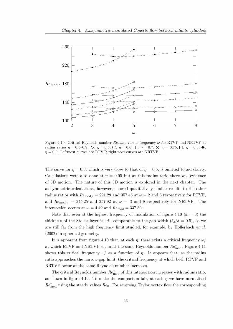
Chapter 4. Axisymmetric modulated Couette flow between infinite cylinders
100
140
180
220
260
2 3 4 5 6 7 8
Remod,c
ω
Figure 4.10: Critical Reynolds number Remod,c versus frequency ω for RTVF and NRTVF atradius ratios η = 0.5–0.9. : η = 0.5, : η = 0.6, : η = 0.7, : η = 0.75, : η = 0.8, :η = 0.9. Leftmost curves are RTVF; rightmost curves are NRTVF.
The curve for η = 0.3, which is very close to that of η = 0.5, is omitted to aid clarity.
Calculations were also done at η = 0.95 but at this radius ratio there was evidence
of 3D motion. The nature of this 3D motion is explored in the next chapter. The
axisymmetric calculations, however, showed qualitatively similar results to the other
radius ratios with Remod,c = 291.29 and 357.45 at ω = 2 and 5 respectively for RTVF,
and Remod,c = 345.25 and 357.92 at ω = 3 and 8 respectively for NRTVF. The
intersection occurs at ω = 4.49 and Remod = 337.80.
Note that even at the highest frequency of modulation of figure 4.10 (ω = 8) the
thickness of the Stokes layer is still comparable to the gap width (δs/δ = 0.5), so we
are still far from the high frequency limit studied, for example, by Hollerbach et al.
(2002) in spherical geometry.
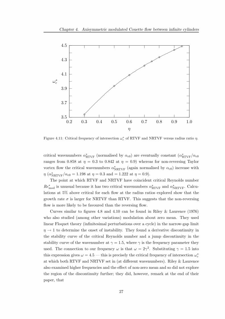
It is apparent from figure 4.10 that, at each η, there exists a critical frequency ω∗c
at which RTVF and NRTVF set in at the same Reynolds number Re∗mod. Figure 4.11
shows this critical frequency ω∗c as a function of η. It appears that, as the radius
ratio approaches the narrow-gap limit, the critical frequency at which both RTVF and
NRTVF occur at the same Reynolds number increases.
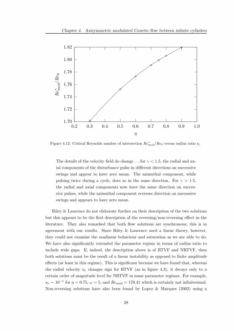
The critical Reynolds number Re∗mod of this intersection increases with radius ratio,
as shown in figure 4.12. To make the comparison fair, at each η we have normalised
Re∗mod using the steady values Re0. For reversing Taylor vortex flow the corresponding
26
Chapter 4. Axisymmetric modulated Couette flow between infinite cylinders
3.5
3.7
3.9
4.1
4.3
4.5
0.2 0.3 0.4 0.5 0.6 0.7 0.8 0.9 1.0
ω∗c
η
Figure 4.11: Critical frequency of intersection ω∗
c of RTVF and NRTVF versus radius ratio η.
critical wavenumbers α∗RTVF (normalised by αc0) are eventually constant (α∗
RTVF/αc0
ranges from 0.858 at η = 0.3 to 0.842 at η = 0.9) whereas for non-reversing Taylor
vortex flow the critical wavenumbers α∗NRTVF (again normalised by αc0) increase with
η (α∗NRTVF/αc0 = 1.198 at η = 0.3 and = 1.222 at η = 0.9).
The point at which RTVF and NRTVF have coincident critical Reynolds number
Re∗mod is unusual because it has two critical wavenumbers α∗RTVF and α∗
NRTVF. Calcu-
lations at 5% above critical for each flow at the radius ratios explored show that the
growth rate σ is larger for NRTVF than RTVF. This suggests that the non-reversing
flow is more likely to be favoured than the reversing flow.
Curves similar to figures 4.8 and 4.10 can be found in Riley & Laurence (1976)
who also studied (among other variations) modulation about zero mean. They used
linear Floquet theory (infinitesimal perturbations over a cycle) in the narrow-gap limit
η → 1 to determine the onset of instability. They found a derivative discontinuity in
the stability curve of the critical Reynolds number and a jump discontinuity in the
stability curve of the wavenumber at γ = 1.5, where γ is the frequency parameter they
used. The connection to our frequency ω is that ω = 2γ2. Substituting γ = 1.5 into
this expression gives ω = 4.5 — this is precisely the critical frequency of intersection ω∗c
at which both RTVF and NRTVF set in (at different wavenumbers). Riley & Laurence
also examined higher frequencies and the effect of non-zero mean and so did not explore
the region of the discontinuity further; they did, however, remark at the end of their
paper, that
27
Chapter 4. Axisymmetric modulated Couette flow between infinite cylinders
1.70
1.72
1.74
1.76
1.78
1.80
1.82
0.2 0.3 0.4 0.5 0.6 0.7 0.8 0.9 1.0
Re∗ m
od/R
e0
η
Figure 4.12: Critical Reynolds number of intersection Re∗
mod/Re0 versus radius ratio η.
The details of the velocity field do change . . . for γ < 1.5, the radial and ax-
ial components of the disturbance pulse in different directions on successive
swings and appear to have zero mean. The azimuthal component, while
pulsing twice during a cycle, does so in the same direction. For γ > 1.5,
the radial and axial components now have the same direction on succes-
sive pulses, while the azimuthal component reverses direction on successive
swings and appears to have zero mean.
Riley & Laurence do not elaborate further on their description of the two solutions
but this appears to be the first description of the reversing/non-reversing effect in the
literature. They also remarked that both flow solutions are synchronous; this is in
agreement with our results. Since Riley & Laurence used a linear theory, however,
they could not examine the nonlinear behaviour and saturation as we are able to do.
We have also significantly extended the parameter regime in terms of radius ratio to
include wide gaps. If, indeed, the description above is of RTVF and NRTVF, then
both solutions must be the result of a linear instability as opposed to finite amplitude
effects (at least in this regime). This is significant because we have found that, whereas
the radial velocity ur changes sign for RTVF (as in figure 4.3), it decays only to a
certain order of magnitude level for NRTVF in some parameter regimes. For example,
ur ∼ 10−1 for η = 0.75, ω = 5, and Remod = 170.41 which is certainly not infinitesimal.
Non-reversing solutions have also been found by Lopez & Marques (2002) using a
28

Chapter 4. Axisymmetric modulated Couette flow between infinite cylinders
Floquet theory for modulation of the outer cylinder’s rotation.
Subsequent work on modulated Couette flow was done by Carmi & Tustaniwskyj
(1981) who also used a linear Floquet theory. They did not detect the existence of
the discontinuities in the stability curves found by Riley & Laurence nor did they
mention differences in flow solutions. They attributed this discrepancy partially to an
approximation in the theory made by Riley & Laurence that they claimed is invalid
in the modulated case. In the related problem of modulation around non-zero mean,
however, their results were later shown to be in error by Barenghi & Jones (1989) who
conjectured that they had used too large a time step. It appears that this time step was
used in all their calculations and, if this is the case, then it may not be possible to draw
any meaningful conclusions from the fact that they did not find the discontinuity. The
time step is especially important in the modulated case because the velocities can decay
to very small values when the time-dependent Reynolds number becomes subcritical
during the cycle. When the frequency is very low this issue is an even greater factor
because the solution has longer to decay. If the time step is too large then the small
velocities are not computed accurately enough.
It is important to note that the existence of either flow is not a consequence of
the initial seeding conditions we use in our numerical code. In the steady-state case,
and using periodic boundary conditions (with the constraint that uz = 0 at the ends
of our computational domain), the bifurcation to a cellular flow (Taylor vortex flow)
is a pitchfork, with one branch corresponding to cells which rotate in one direction,
and the other branch corresponding to cells rotating in the opposite direction. The
smooth transition to a cellular flow is due to some seeding ‘noise’ which breaks the
perfect pitchfork bifurcation symmetry. Changing the sign of this noise would select the
opposite branch. The initial seeding noise is necessary to start up the flow and changing
the sign of the initial condition merely changes the direction of rotation of the first cell.
We cannot use the above argument in our modulated problem. The Reynolds number
changes sign periodically, and the flow is a time-dependent solution of the Navier–Stokes
equation which develops self-consistently, independently of some arbitrary noise. As
shown in figures 5.5 and 5.8 in chapter 5, depending on the parameters, this flow is
different in the reversing and non-reversing cases. The situation is the same in a related
time-dependent problem (Lopez & Marques, 2002).
4.1.3 Wavy modes
The preceding calculations were performed including a sufficient level of truncation so
as to capture any possible three-dimensional nature of the flow. Azimuthal spectral
truncations as high as M = 8 were used. In all cases the flow was always found to be
axisymmetric.
29
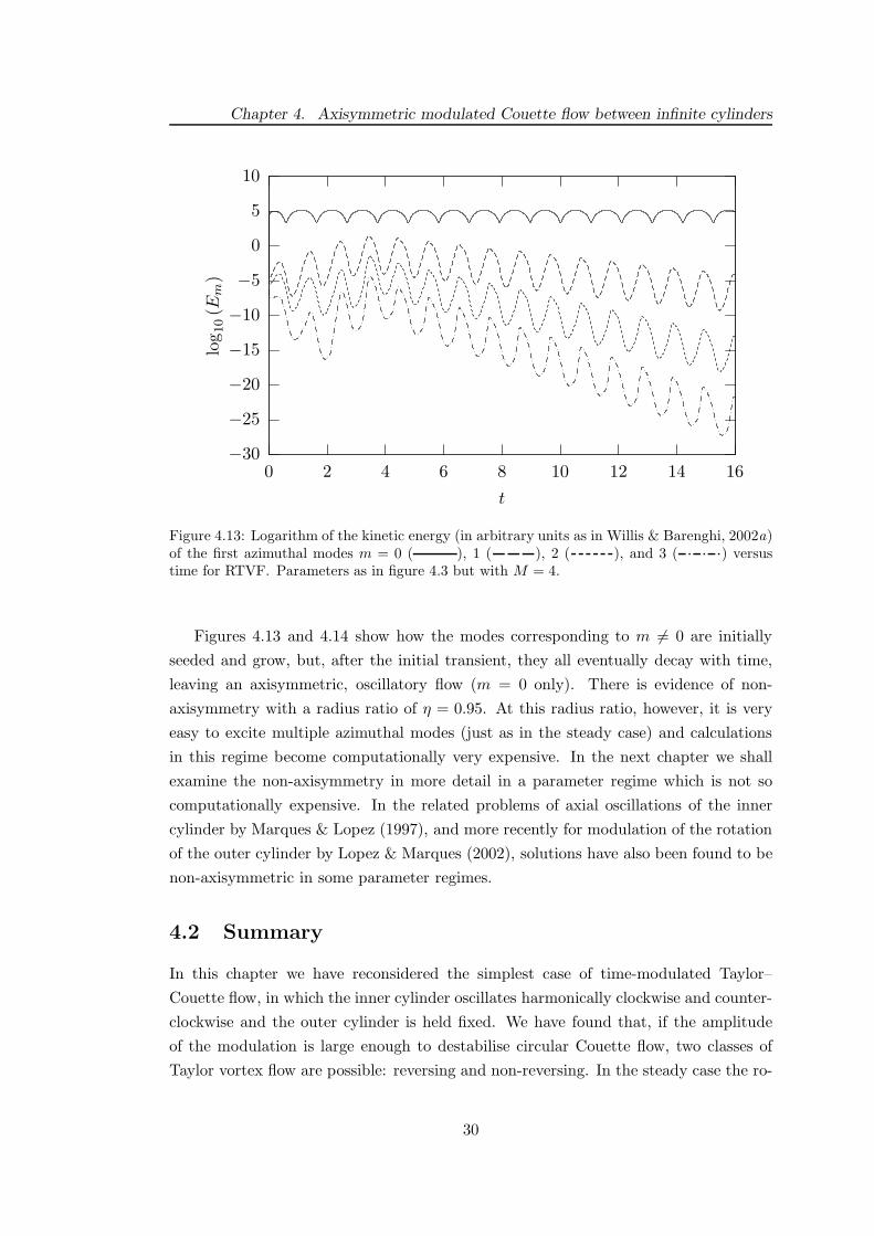
Chapter 4. Axisymmetric modulated Couette flow between infinite cylinders
−30
−25
−20
−15
−10
−5
0
5
10
0 2 4 6 8 10 12 14 16
log
10(E
m)
t
Figure 4.13: Logarithm of the kinetic energy (in arbitrary units as in Willis & Barenghi, 2002a)of the first azimuthal modes m = 0 ( ), 1 ( ), 2 ( ), and 3 ( ) versustime for RTVF. Parameters as in figure 4.3 but with M = 4.
Figures 4.13 and 4.14 show how the modes corresponding to m 6= 0 are initially
seeded and grow, but, after the initial transient, they all eventually decay with time,
leaving an axisymmetric, oscillatory flow (m = 0 only). There is evidence of non-
axisymmetry with a radius ratio of η = 0.95. At this radius ratio, however, it is very
easy to excite multiple azimuthal modes (just as in the steady case) and calculations
in this regime become computationally very expensive. In the next chapter we shall
examine the non-axisymmetry in more detail in a parameter regime which is not so
computationally expensive. In the related problems of axial oscillations of the inner
cylinder by Marques & Lopez (1997), and more recently for modulation of the rotation
of the outer cylinder by Lopez & Marques (2002), solutions have also been found to be
non-axisymmetric in some parameter regimes.
4.2 Summary
In this chapter we have reconsidered the simplest case of time-modulated Taylor–
Couette flow, in which the inner cylinder oscillates harmonically clockwise and counter-
clockwise and the outer cylinder is held fixed. We have found that, if the amplitude
of the modulation is large enough to destabilise circular Couette flow, two classes of
Taylor vortex flow are possible: reversing and non-reversing. In the steady case the ro-
30
Chapter 4. Axisymmetric modulated Couette flow between infinite cylinders
−25
−20
−15
−10
−5
0
5
10
0 2 4 6 8 10 12 14 16
log
10(E
m)
t
Figure 4.14: Logarithm of the kinetic energy (in arbitrary units as in Willis & Barenghi, 2002a)of the first azimuthal modes m = 0 ( ), 1 ( ), 2 ( ), and 3 ( ) versustime for NRTVF. Parameters as in figure 4.6 but with M = 4.
tation direction of the Taylor vortices is not influenced by the rotation direction of the
inner cylinder. There is no reason to suggest that the situation should be any different
in the modulated case since the inner cylinder spends an equal period of time rotating
in both clockwise and counter-clockwise directions. NRTVF is most consistent with
this view — the vortices do not alter their rotation direction when the inner cylinder
does. In contrast to this, however, the rotation direction of the Taylor cells in RTVF
does depend on the rotation direction of the inner cylinder, so when the inner cylinder
changes its rotation direction so do the Taylor cells. NRTVF takes place at sufficiently
high modulation frequencies for which there is not enough time for the toroidal motion
to vanish to sufficiently small values (still these frequencies are small enough that δs is
comparable to δ).
In the next chapter we continue our discussion of reversing and non-reversing Taylor
vortex flow but we allow for non-axisymmetric motion and the existence of wavy modes.
31
Chapter 5
Non-axisymmetric modulated
Couette flow between infinite
cylinders
It is well known that, in the steady Taylor–Couette problem, if the Reynolds number Re
is sufficiently larger than Re0, at some critical value which depends on the radius ratio,
Taylor vortex flow (TVF) loses its azimuthal symmetry and becomes time-dependent
wavy modes (WM). In the modulated Taylor–Couette problem the natural question
to ask is thus whether or not the appearance of the wavy modes instability in the
θ-direction destroys the existence of non-reversing solutions. Is there a distinction
between reversing and non-reversing wavy modes (RWM and NRWM) similar to the
distinction between RTVF and NRTVF? We are thus lead to the study of what happens
at large amplitudes of modulation Remod.
Because of the large computational costs of solving the Navier–Stokes equations
in the wavy modes regime, we do not attempt to determine the stability boundary of
possible non-reversing wavy flows (which would require minimising Remod as a function
of α), but restrict our task to determining the existence (or non-existence) of non-
reversing wavy flows.
5.1 Non-axisymmetric reversing and non-reversing flows
It is important to note that, in the wavy modes regime, a change of sign of ur versus r
at fixed z during the time evolution is not enough to guarantee that a reversal has taken
place. This is because in the wavy modes regime the Taylor vortices oscillate up and
down in the axial z direction, so the value of ur at a fixed location in the (r, z)-plane
can change sign even when a reversal is not taking place. To counteract this effect we
32
Chapter 5. Non-axisymmetric modulated Couette flow between infinite cylinders
2πα
0
z
Figure 5.1: Contour plot of radial velocity ur for non-axisymmetric non-reversing flow at afixed azimuthal position. Choosing a different azimuthal position has the effect of shifting thecells up or down slightly in the axial direction. Note the trapezoidal deformation. Dashed linesrepresent positive ur, solid lines represent negative ur.
plot ur versus r in a frame of reference moving with a particular vortex, tracking the
location where ur is maximal/minimal within the entire Taylor vortex cell. If the flow
is non-reversing then the profile of ur computed in this way is always positive/negative.
If the flow is reversing then the profile of ur is positive for the first part of the cycle
and negative for the second part (or vice-versa), with a smooth transition between the
two as the nodal line crosses the gap.
The reason for tracking the maximal/minimal value of ur over the entire Taylor
vortex cell is that, if the axial position is fixed, then it is still possible for ur to be
positive in one part of the gap but negative in another. This is because of deformations
of the Taylor vortex cells from a square to trapezoidal shape which occurs during the
evolution. An example of this deformation can be seen in figure 5.1.
The figure shows a vertical cross-section of the radial velocity through a pair of
Taylor vortices. The inner cylinder is on the left and the outer cylinder on the right.
The plot extends to one wavelength, λ = 2π/α in the axial direction. It can clearly be
seen that at z ≈ 3π/2α and z ≈ π/2α, where the radial velocity changes sign in the
axial direction, it also changes sign in the radial direction. A plot of ur against time
would then suggest that a reversal had occurred, which is not the case.
Having taken these necessary precautions, plots of ur versus r computed as de-
scribed can reveal whether a flow is reversing or non-reversing. Figure 5.2 shows a
reversing flow for example at η = 0.8, ω = 4, and Remod = 250. Here, we see the radial
33

Chapter 5. Non-axisymmetric modulated Couette flow between infinite cylinders
0.0 0.2 0.4 0.6 0.8 1.0r 195.70
195.71195.72
195.73195.74
195.75
t
−0.006
−0.004
−0.002
0.000
0.002
ur
Figure 5.2: Radial velocity ur computed by tracking the Taylor vortex as explained in the text,versus radial position r for non-axisymmetric reversing flow (η = 0.8, ω = 4, Remod = 250).Each curve is plotted for a different time with 195.704 6 t 6 195.749. The curves show ur < 0,initially, and ur > 0 after the nodal line has crossed the gap. The filled circles indicate theradial position where ur = 0.
velocity versus radial position at nine different times when the actual reversal takes
place. The curves should be read from the bottom (where ur < 0) to the top (where
ur > 0) with time increasing in that direction. Initially, ur is negative everywhere
across the gap. As time progresses, however, ur becomes positive in parts of the gap
(shown by the dashed parts of the curve in the figure), until eventually ur is positive
everywhere within the gap, as the new vortices appear from the inner cylinder. The
filled circles, which mark the location where ur = 0, represent the passage of the nodal
line across the gap, hence prove that a reversal has taken place. The three contour plots
of ur in the (r, z)-plane over a full wavelength at fixed θ shown in figure 5.3 capture
the passage of the nodal line.
In 5.3(a) we have a radial inflow at the centre-line at t = 195.704, at (b) we have
four vortices within the gap at t = 195.726, and finally, at (c) we now have a radial
outflow at the centre-line at t = 195.749. The whole reversal process is completed in
only hundredths of a diffusion time.
Figure 5.4 shows a time-series plot of the radial velocity ur over two forcing periods
for the non-axisymmetric reversing flow. The period of the forcing is T = 2π/ω which
is 1.57 for the frequency of ω = 4 shown. The reversing flow responds to this forcing
synchronously and also has a period of 1.57. This synchronous response was also found
34
Chapter 5. Non-axisymmetric modulated Couette flow between infinite cylinders
2πα
0
z
(a)
(b)
(c)
Figure 5.3: Contours of the radial velocity component for non-axisymmetric reversing flow atone particular azimuthal position. (a) at t = 195.704, (b) at t = 195.726, (c) at t = 195.749.Dashed lines represent positive ur, solid lines represent negative ur.
in the axisymmetric regime of chapter 4, and is again in contrast to the (axisymmetric)
results of Lopez & Marques (2002) who, in modulated Taylor–Couette flow with a
constantly rotating inner cylinder and sinusoidally modulated outer cylinder, found
that the reversing solutions were subharmonic with a period of twice that of the forcing.
Figure 5.5 shows 3D perspective views of the non-axisymmetric reversing flow at
four different times during a cycle. Values of the instantaneous Reynolds number and
radial velocity at these times can be seen from the time-series plot of the radial velocity,
figure 5.4. Shown are isosurfaces of helicity H = |u · (∇ ∧ u)| over two axial periods.
It is apparent that the flow is predominantly m = 1, only looking the same after a full
360 rotation about the axis. In chapter 4 we found that there is a phase-lag between
the change of rotation direction of the inner cylinder and when the flow intensity is at
a minimum, because the flow across the gap takes a certain amount of time to respond
to the drive. Consequently, where figures 5.5(b) and (c) show the flow intensity at
a minimum, the instantaneous Reynolds number is not close to zero. Helicity is a
convenient quantity to represent the flow graphically, since it highlights the location of
the Taylor vortex cells behind the layer of vorticity near the outer cylinder. It should
be noted that there is a contribution from the helicity on the inner cylinder which is
visible in the figures, but which does not obscure the cellular structure.
Figure 5.6 shows radial profiles as in figure 5.2 but now for a case which corresponds
35
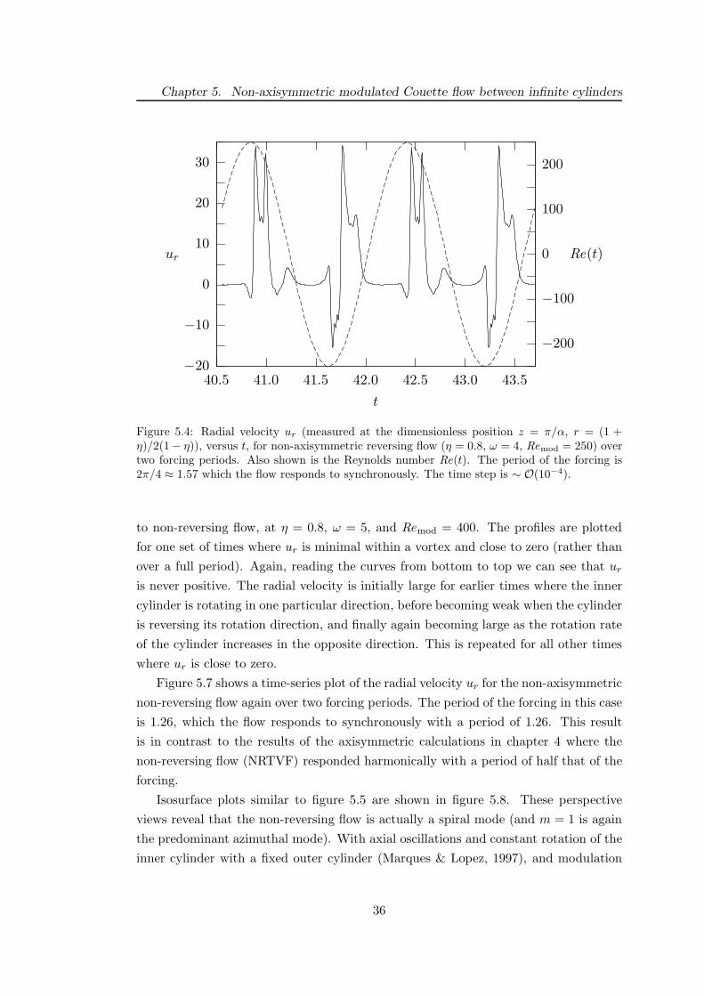
Chapter 5. Non-axisymmetric modulated Couette flow between infinite cylinders
−20
−10
0
10
20
30
40.5 41.0 41.5 42.0 42.5 43.0 43.5
−200
−100
0
100
200
ur Re(t)
t
Figure 5.4: Radial velocity ur (measured at the dimensionless position z = π/α, r = (1 +η)/2(1− η)), versus t, for non-axisymmetric reversing flow (η = 0.8, ω = 4, Remod = 250) overtwo forcing periods. Also shown is the Reynolds number Re(t). The period of the forcing is2π/4 ≈ 1.57 which the flow responds to synchronously. The time step is ∼ O(10−4).
to non-reversing flow, at η = 0.8, ω = 5, and Remod = 400. The profiles are plotted
for one set of times where ur is minimal within a vortex and close to zero (rather than
over a full period). Again, reading the curves from bottom to top we can see that ur
is never positive. The radial velocity is initially large for earlier times where the inner
cylinder is rotating in one particular direction, before becoming weak when the cylinder
is reversing its rotation direction, and finally again becoming large as the rotation rate
of the cylinder increases in the opposite direction. This is repeated for all other times
where ur is close to zero.
Figure 5.7 shows a time-series plot of the radial velocity ur for the non-axisymmetric
non-reversing flow again over two forcing periods. The period of the forcing in this case
is 1.26, which the flow responds to synchronously with a period of 1.26. This result
is in contrast to the results of the axisymmetric calculations in chapter 4 where the
non-reversing flow (NRTVF) responded harmonically with a period of half that of the
forcing.
Isosurface plots similar to figure 5.5 are shown in figure 5.8. These perspective
views reveal that the non-reversing flow is actually a spiral mode (and m = 1 is again
the predominant azimuthal mode). With axial oscillations and constant rotation of the
inner cylinder with a fixed outer cylinder (Marques & Lopez, 1997), and modulation
36
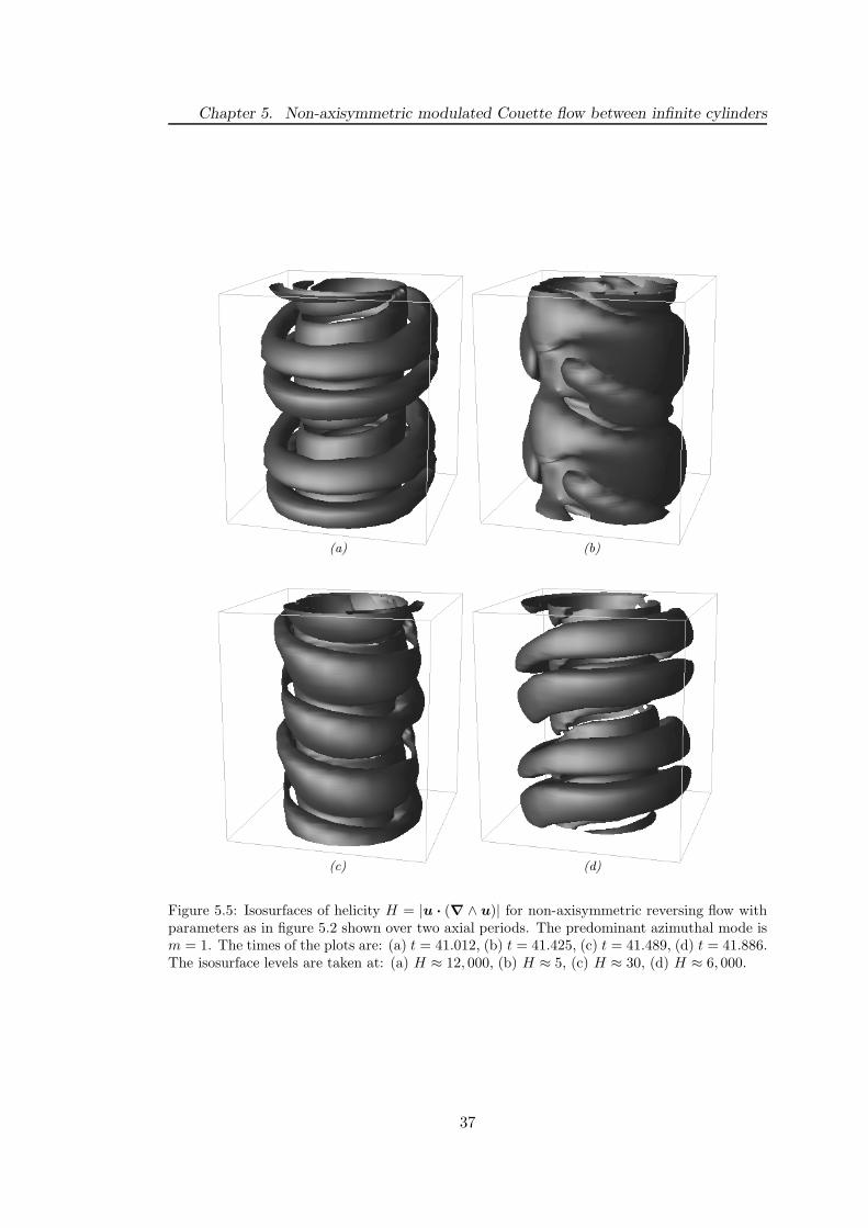
Chapter 5. Non-axisymmetric modulated Couette flow between infinite cylinders
(a) (b)
(c) (d)
Figure 5.5: Isosurfaces of helicity H = |u · (∇ ∧ u)| for non-axisymmetric reversing flow withparameters as in figure 5.2 shown over two axial periods. The predominant azimuthal mode ism = 1. The times of the plots are: (a) t = 41.012, (b) t = 41.425, (c) t = 41.489, (d) t = 41.886.The isosurface levels are taken at: (a) H ≈ 12, 000, (b) H ≈ 5, (c) H ≈ 30, (d) H ≈ 6, 000.
37
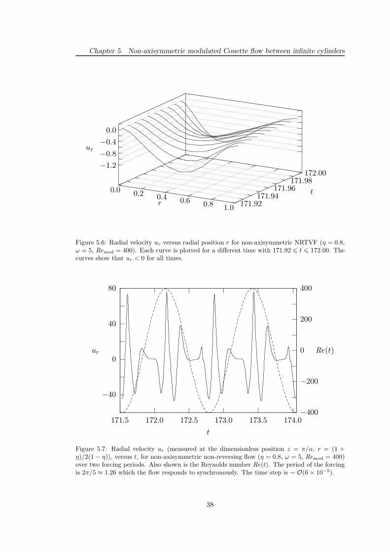
Chapter 5. Non-axisymmetric modulated Couette flow between infinite cylinders
0.0 0.2 0.4 0.6 0.8 1.0 171.92171.94
171.96171.98
172.00−1.2
−0.8
−0.4
0.0
ur
r
t
Figure 5.6: Radial velocity ur versus radial position r for non-axisymmetric NRTVF (η = 0.8,ω = 5, Remod = 400). Each curve is plotted for a different time with 171.92 6 t 6 172.00. Thecurves show that ur < 0 for all times.
−40
0
40
80
171.5 172.0 172.5 173.0 173.5 174.0−400
−200
0
200
400
ur Re(t)
t
Figure 5.7: Radial velocity ur (measured at the dimensionless position z = π/α, r = (1 +η)/2(1 − η)), versus t, for non-axisymmetric non-reversing flow (η = 0.8, ω = 5, Remod = 400)over two forcing periods. Also shown is the Reynolds number Re(t). The period of the forcingis 2π/5 ≈ 1.26 which the flow responds to synchronously. The time step is ∼ O(6 × 10⁻⁵).
38
Chapter 5. Non-axisymmetric modulated Couette flow between infinite cylinders
of the outer cylinder with a constant rotation of the inner cylinder (Lopez & Marques,
2002), it was found that Neimark–Sacker bifurcations to a quasiperiodic solution were
possible. Lopez & Marques found that the Neimark–Sacker bifurcation results in the
formation of a family of spiral solutions, a left-hand spiral with azimuthal wavenumber
+m, and a right-hand spiral with azimuthal wavenumber −m. They found that these
spirals precess in the same sense as the cylinder rotation, but much slower, and also
remarked that these solutions are generally quasiperiodic, but that strong resonances
are found along the Neimark–Sacker curve. In our case we have found that the spiral
also precesses in the same sense as the inner cylinder rotation but at the same rate.
Poincare sections reveal that the flow is periodic, and a Fourier transform of the radial
and axial velocities reveal that there is only one frequency in the solution — that of the
forcing frequency. There is no evidence of quasiperiodic motion in our case. Indeed,
we should not expect quasiperiodic motion since the inner cylinder spends an equal
amount of time rotating both clockwise and counter-clockwise.
Figure 5.9 confirms that we are indeed dealing with a non-axisymmetric flow (cf.
figures 4.3 and 4.6 in chapter 4). The figure shows the contribution of each wavy mode
component (m = 0, 1, 2, . . .) to the total kinetic energy plotted versus time for a
reversing flow (plots for non-reversing flows are similar). We can see that the kinetic
energy of the wavy modes does not decay after the initial seeding. To aid clarity only
the first three non-axisymmetric modes are shown, but the calculation includes spectral
truncations of up to M = 8 in the azimuthal direction. A few words on the choice of
radius ratio and truncation for the non-axisymmetric flows are relevant at this point.
Jones (1985b) found that, in the steady case, as the narrow-gap limit is approached, it
becomes easier to excite modes with higher and higher azimuthal wavenumber. This
is also true in our modulated case and thus fully-resolved 3-dimensional calculations in
the narrow-gap limit η → 1 require CPU times too large to be practical. On the other
hand, if the radius ratio is too small — but not so small as to be out of the (steady)
wavy regime, η < 0.70, say — then due to the large modulation amplitudes involved,
the Reynolds number is not in the wavy regime for long enough and the wavy modes
decay quickly. Consequently, finding a convenient regime to study in which wavy modes
exist is a balancing act between azimuthal truncation at narrow gaps and exciting the
azimuthal modes in wider gaps.
5.2 Summary
The goal of this chapter was to extend the axisymmetric investigation of chapter 4 into
the non-axisymmetric regime to see whether the presence of an azimuthal instability
would lead to the existence of reversing and non-reversing wavy modes. Calculations in
39
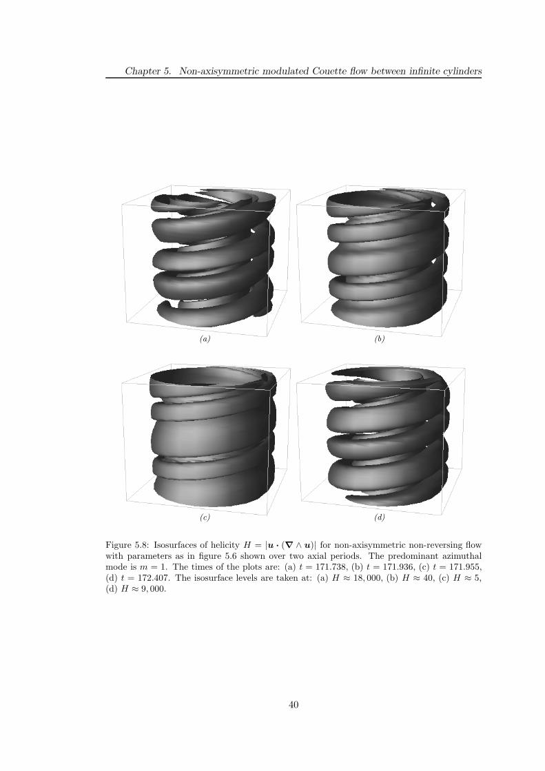
Chapter 5. Non-axisymmetric modulated Couette flow between infinite cylinders
(a) (b)
(c) (d)
Figure 5.8: Isosurfaces of helicity H = |u · (∇ ∧ u)| for non-axisymmetric non-reversing flowwith parameters as in figure 5.6 shown over two axial periods. The predominant azimuthalmode is m = 1. The times of the plots are: (a) t = 171.738, (b) t = 171.936, (c) t = 171.955,(d) t = 172.407. The isosurface levels are taken at: (a) H ≈ 18, 000, (b) H ≈ 40, (c) H ≈ 5,(d) H ≈ 9, 000.
40
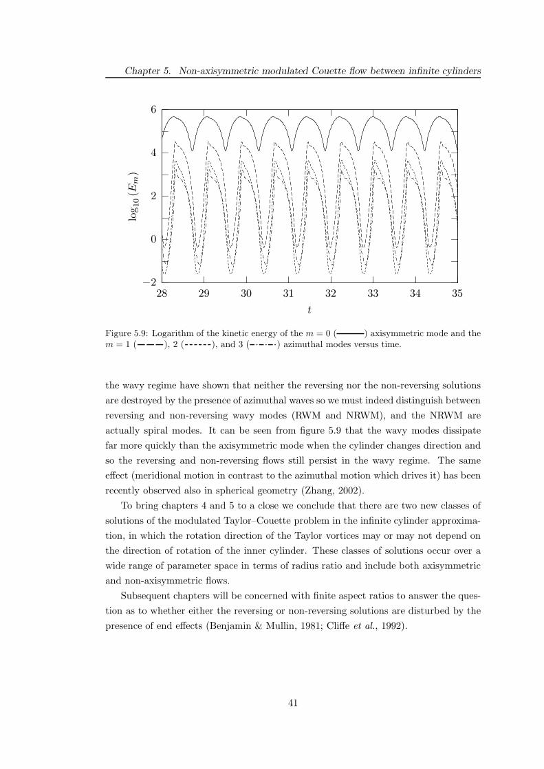
Chapter 5. Non-axisymmetric modulated Couette flow between infinite cylinders
−2
0
2
4
6
28 29 30 31 32 33 34 35
log
10(E
m)
t
Figure 5.9: Logarithm of the kinetic energy of the m = 0 ( ) axisymmetric mode and them = 1 ( ), 2 ( ), and 3 ( ) azimuthal modes versus time.
the wavy regime have shown that neither the reversing nor the non-reversing solutions
are destroyed by the presence of azimuthal waves so we must indeed distinguish between
reversing and non-reversing wavy modes (RWM and NRWM), and the NRWM are
actually spiral modes. It can be seen from figure 5.9 that the wavy modes dissipate
far more quickly than the axisymmetric mode when the cylinder changes direction and
so the reversing and non-reversing flows still persist in the wavy regime. The same
effect (meridional motion in contrast to the azimuthal motion which drives it) has been
recently observed also in spherical geometry (Zhang, 2002).
To bring chapters 4 and 5 to a close we conclude that there are two new classes of
solutions of the modulated Taylor–Couette problem in the infinite cylinder approxima-
tion, in which the rotation direction of the Taylor vortices may or may not depend on
the direction of rotation of the inner cylinder. These classes of solutions occur over a
wide range of parameter space in terms of radius ratio and include both axisymmetric
and non-axisymmetric flows.
Subsequent chapters will be concerned with finite aspect ratios to answer the ques-
tion as to whether either the reversing or non-reversing solutions are disturbed by the
presence of end effects (Benjamin & Mullin, 1981; Cliffe et al., 1992).
41
Chapter 6
Anomalous modes
So far we have looked at the case in which the cylinders are assumed to be infinite so
that end effects can be ignored. The calculations assuming this condition are extremely
helpful in gaining an insight into the results observed in experiments. This approxi-
mation is valid when the cylinders are very long but as we have already mentioned in
the introduction, end effects cannot be ignored when the condition Γ δ/R1 is not
satisfied.
The work of Benjamin (1978a,b); Benjamin & Mullin (1981); Cliffe (1983); Bolstad
& Keller (1987); Pfister et al. (1988); Cliffe et al. (1992); Mullin et al. (2002); Furukawa
et al. (2002); Lopez & Marques (2003) has shown that end effects play a key role in
selecting the steady cellular vortex pattern and that an important parameter of the
problem is the aspect ratio Γ (the ratio of the height of the cylinders to the width
of the gap). There are generally two options to consider when working with finite
cylinders. The first is the case where the end-plates are attached to the inner cylinder
and so rotate with it (see, for example, Tavener et al., 1991); here, it is found that the
cells closest to the ends rotate in such a way so as to give rise to a radial outflow at the
endwalls. The second is the case where the end-plates are attached to the (stationary)
outer cylinder, and this is the case we shall be concentrating on for the rest of this thesis;
here, it is found that there is usually a radial inflow at the endwalls (but see below).
Other possibilities for the arrangement of the end-plates include one rotating end and
one fixed end (see, for example, Mullin & Blohm, 2001). The existence of the (fixed)
ends gives rise to the so-called ‘anomalous’ modes where the cells close to the ends
have a direction of rotation which is apparently opposite to what is initially expected.
The classical thinking is that the centrifugal force exerted by the rotation of the inner
cylinder pushes the fluid outwards at mid-height due to the braking effect of the ends,
then, to conserve mass, the fluid must flow inwards near the ends. The ‘anomalous’
modes appear to have an outflow at one or both of the ends; closer inspection reveals
the existence of small vortices in the corners near to the inner cylinder (in fact, in
42
Chapter 6. Anomalous modes
some cases it is possible for there to be small vortices in the corners next to the outer
cylinder as well), but the name ‘anomalous’ has not been changed and has remained in
the literature to distinguish this remarkable flow pattern. We define the primary flow
to be that developed as the Reynolds number is gradually increased from values small
enough for the flow to be unique (Benjamin, 1978b), and then in terms of bifurcation
theory, anomalous modes are always disconnected from the primary flow and appear
at Reynolds numbers much higher (sometimes an order of magnitude higher) than the
threshold for normal modes; only one exception is known: as the aspect ratio is reduced
such that the height of the cylinders is of the order of the gap between the cylinders,
an anomalous 1-cell state is found which is connected to the primary flow and can be
realised by a quasi-static increase in the Reynolds number.
Figure 6.1(a) shows an example of a 3-cell anomalous mode. Plotted is the stream
function ψ, equation (4.1). The inner cylinder is on the left and the aspect ratio is
Γ = 3, so that there are three full-size cells and a small cell in the top corner. In
this case there is radial inflow at the bottom boundary z = 0 and what would appear
to be outflow at the top boundary z = Γ = 3. The presence of the small cell in the
corner next to the inner cylinder, however, ensures that there is in fact radial inflow at
this boundary. There is actually a small cell in the opposite corner next to the outer
cylinder as well, but this is very much weaker than the other vortices. Consequently,
this extra cell never appears on any contour plots. The vortices are asymmetric about
the midplane, and this is the most likely situation whenever the aspect ratio is odd.
A mirror image flow obtained by reflecting about the midplane is also possible for
anomalous modes with an odd number of cells. Which of the two forms of solution
is found depends on the sign of the initial condition. Figure 6.1(b) shows a 4-cell
anomalous mode. In this case Γ = 4. Now there are four full-size vortices and two
smaller cells in the top and bottom corners near to the inner cylinder. Here, there
is radial outflow at the midplane, suggesting radial outflow at the top and bottom
ends; the presence of the small cells in the corners close to the inner cylinder, however,
ensures that we have radial inflow at the boundaries. In this case there are also extra
cells in the corners next to the outer cylinder but again, they never show up in contour
plots. In contrast to any anomalous mode with an odd number of cells, anomalous
modes with an even number of cells are symmetric about the midplane. This is the
case whenever the aspect ratio is even.
Strictly speaking, we should not call these examples 3- and 4-cell anomalous modes
because they actually have 4 and 6 cells respectively, although of different sizes. Never-
theless, the terminology has stuck and has become standard in the literature. Whenever
we describe anomalous modes with an odd number of cells we are actually referring to
the number of large, fully formed cells.
43

Chapter 6. Anomalous modes
3
z
0
(a)
4
0
(b)
Figure 6.1: Taylor–Couette flow at finite aspect ratio, η = 0.615. (a) 3-cell anomalous modewith Γ = 3, Re = 240 and (b) 4-cell anomalous mode with Γ = 4, Re = 240.
44
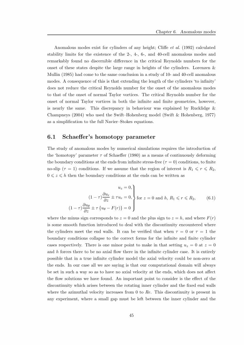
Chapter 6. Anomalous modes
Anomalous modes exist for cylinders of any height; Cliffe et al. (1992) calculated
stability limits for the existence of the 2-, 4-, 6-, and 40-cell anomalous modes and
remarkably found no discernible difference in the critical Reynolds numbers for the
onset of these states despite the large range in heights of the cylinders. Lorenzen &
Mullin (1985) had come to the same conclusion in a study of 10- and 40-cell anomalous
modes. A consequence of this is that extending the length of the cylinders ‘to infinity’
does not reduce the critical Reynolds number for the onset of the anomalous modes
to that of the onset of normal Taylor vortices. The critical Reynolds number for the
onset of normal Taylor vortices in both the infinite and finite geometries, however,
is nearly the same. This discrepancy in behaviour was explained by Rucklidge &
Champneys (2004) who used the Swift–Hohenberg model (Swift & Hohenberg, 1977)
as a simplification to the full Navier–Stokes equations.
6.1 Schaeffer’s homotopy parameter
The study of anomalous modes by numerical simulations requires the introduction of
the ‘homotopy’ parameter τ of Schaeffer (1980) as a means of continuously deforming
the boundary conditions at the ends from infinite stress-free (τ = 0) conditions, to finite
no-slip (τ = 1) conditions. If we assume that the region of interest is R1 6 r 6 R2,
0 6 z 6 h then the boundary conditions at the ends can be written as
uz = 0,
(1 − τ)∂ur
∂z± τur = 0,
(1 − τ)∂uθ
∂z± τ uθ − F (r) = 0
for z = 0 and h, R1 6 r 6 R2, (6.1)
where the minus sign corresponds to z = 0 and the plus sign to z = h, and where F (r)
is some smooth function introduced to deal with the discontinuity encountered where
the cylinders meet the end walls. It can be verified that when τ = 0 or τ = 1 the
boundary conditions collapse to the correct forms for the infinite and finite cylinder
cases respectively. There is one minor point to make in that setting uz = 0 at z = 0
and h forces there to be no axial flow there in the infinite cylinder case. It is entirely
possible that in a true infinite cylinder model the axial velocity could be non-zero at
the ends. In our case all we are saying is that our computational domain will always
be set in such a way so as to have no axial velocity at the ends, which does not affect
the flow solutions we have found. An important point to consider is the effect of the
discontinuity which arises between the rotating inner cylinder and the fixed end walls
where the azimuthal velocity increases from 0 to Re. This discontinuity is present in
any experiment, where a small gap must be left between the inner cylinder and the
45
Chapter 6. Anomalous modes
end walls to prevent a temperature gradient building up, which is what would happen
if the boundaries were allowed to meet. The exact form of the relevant boundary
condition to model this would be very difficult to determine and so many numerical
calculations use a small parameter ε 1 which allows the azimuthal velocity to vary
smoothly between the boundary values along the endwalls. It is also common to use
mesh refinement in the corners but it is generally found that provided the mesh size is
small enough in the corners the disturbance caused by the discontinuity is local to the
corners and does not extend significantly into the fluid. Lucke et al. (1984) remarked
that no anomalies could be found within a distance of 0.2 mm of the corners of their
experimental apparatus with a gap width of δ = 1.126 cm.
6.2 Generating an anomalous mode
Generating an anomalous mode is non-trivial and so below we outline a systematic way
of finding an anomalous mode in our new numerical code as described in chapter 7.
Details on how to generate anomalous modes in numerical simulations are also given in
Cliffe & Mullin (1985) and Bolstad & Keller (1987) who used Euler–Newton pseudo-
arclength continuation in their steady solvers. Details on this procedure can be found
in Keller (1977).
To generate an N -cell anomalous mode in our time-dependent code it is first nec-
essary to set Γ = N and τ = 0. In general, Γ need not be an integer, but the following
procedure ensures that the resulting anomalous mode has N cells. Once the anomalous
flow pattern has been established Γ can be continuously altered to any desired value.
The Reynolds number is adjusted to a value just below steady critical Re0 and the
flow is left to decay for a short time to allow an approximate flow structure to appear.
Then, if N is odd, the Reynolds number is increased to a value just above critical and
the flow is left to saturate. If N is even, to produce an anomalous mode we must fol-
low the branch of the ‘perfect’ supercritical pitchfork bifurcation which corresponds to
Taylor vortex flow with radial outflows at the ends. There are standard techniques for
following specific branches at bifurcation points, and in this code it is simply a matter
of switching the sign of the Reynolds number before restarting the time stepping to
ensure that the branch followed is the correct one. The flow is then left to saturate.
After the saturation in both cases of N even and odd, the Reynolds number is in-
creased to some adequately large value that allows the existence of anomalous modes.
If N is even then the Reynolds number is switched sign again and the flow is left to
saturate. At this point τ is continuously varied from 0 to 1 while keeping the Reynolds
number unchanged. Once τ = 1 we have the desired N -cell anomalous mode. Finally,
to find the critical Reynolds number for the onset of the anomalous mode we decrease
46
Chapter 6. Anomalous modes
the Reynolds number until the anomalous mode collapses catastrophically into another
flow pattern. In most cases this new pattern is a normal cell mode; it is possible,
however, that the new flow is another anomalous mode with a different number of cells
to the original. How many cells the new normal or anomalous mode has depends on
whether N is odd or even and on the value of Γ .
6.3 Stability curves
Figure 6.2 shows stability curves for the 2-, 3-, and 4-cell anomalous modes at η = 0.615.
Each curve is calculated separately and so the apparent intersections of the curves
are not significant. For Γ → ∞ and η = 0.615 the critical Reynolds number for
the onset of Taylor vortices is 73, so the size of the Reynolds number shows how far
removed these anomalous modes are from the primary branch of the bifurcation. These
curves were originally experimentally determined by Benjamin & Mullin (1981) but
their critical Reynolds numbers were on the order of 30% lower due to imperfections
in their apparatus. The curves were re-calculated by Cliffe & Mullin (1985) and also
by Bolstad & Keller (1987) where it emerged that the original results were erroneous.
Figure 6.2 was calculated by our numerical code and it agrees well to graphical accuracy
with the results of Cliffe & Mullin and Bolstad & Keller. Bolstad & Keller extended the
curves to include the boundaries for the 5- and 6-cell anomalous modes. They found
that these boundaries had a very unusual shape which is not evident in the curves
for the 2-, 3-, and 4-cell anomalous modes. For the 5- and 6-cell anomalous modes
the left-hand side of the curves was almost vertical leading to a cusp at the lower-left
corner. The right-hand side of the curves was similar to the other anomalous modes.
6.4 Very small aspect ratio
One of the most significant effects of cylinders of finite height is to give rise to non-
unique solutions. Despite all parameters being the same the final flow pattern can
depend strongly on the route taken through parameter space. This was shown strikingly
in the experimental study of Benjamin & Mullin (1982) who demonstrated no fewer
than 39 different steady solutions at the same fixed parameters. They also remarked
that this number could quite probably be increased to 43 but for some difficulties in
experimental control of the apparatus.
To counteract this high degree of multiplicity one solution is to restrict the height
of the cylinders to be on the order of the gap width (so the aspect ratio Γ ≈ 1). In
this very small aspect ratio regime a wide variety of flows have been discovered in-
cluding axisymmetric time-dependent and ‘side-by-side’ flows, depending on the route
taken through parameter space. The final flow pattern can depend strongly on sudden
47

Chapter 6. Anomalous modes
220
260
300
340
380
1.5 2.0 2.5 3.0 3.5 4.0 4.5 5.0 5.5
Re
Γ
Figure 6.2: Stability curves for the 2- ( ), 3- ( ), and 4-cell ( ) anomalousmodes at η = 0.615 for different values of the aspect ratio.
starts of the cylinder or discontinuous jumps of the aspect ratio. For sufficiently small
Reynolds numbers the basic flow is a symmetric 2-cell state composed of an Ekman
circulation induced by the ends. For a large range of aspect ratios the primary bifur-
cation from this 2-cell state is to an asymmetric 1-cell flow comprising one large cell
with a smaller one in the corner next to the inner cylinder. Figure 6.3 shows these
two flow patterns at the same parameters; only the route taken through parameter
space to arrive at these states is different. Much work has been done in the very small
aspect ratio regime and Benjamin & Mullin (1981) were the first to study this regime
experimentally and confirm the existence of the 1- and 2-cell states. They mapped out
the different flow patterns in the (Re, Γ )-plane at η = 0.615. Cliffe (1983) carried out
a numerical study at the same radius ratio and also found the 1- and 2-cell patterns.
At roughly the same time as Cliffe’s work Lucke et al. (1984) numerically and experi-
mentally studied the problem, although they only considered one aspect ratio Γ = 1.05
at η = 0.5066. A further study was carried out by Pfister et al. (1988), at η = 0.5,
who also discovered axisymmetric time-dependent solutions. The works of Benjamin &
Mullin, Cliffe, and Pfister et al. all produced bifurcation diagrams similar to figure 6.4
which shows our own results for the interaction of the 1- and 2-cell states.
Mullin et al. (2002) further explored the parameter space by considering larger
Reynolds numbers and other radius ratios and found bifurcations of 1- and 2-cell flows
(at η = 0.5) for Γ > 0.7. There are also time-dependent flows in this region (which we
48
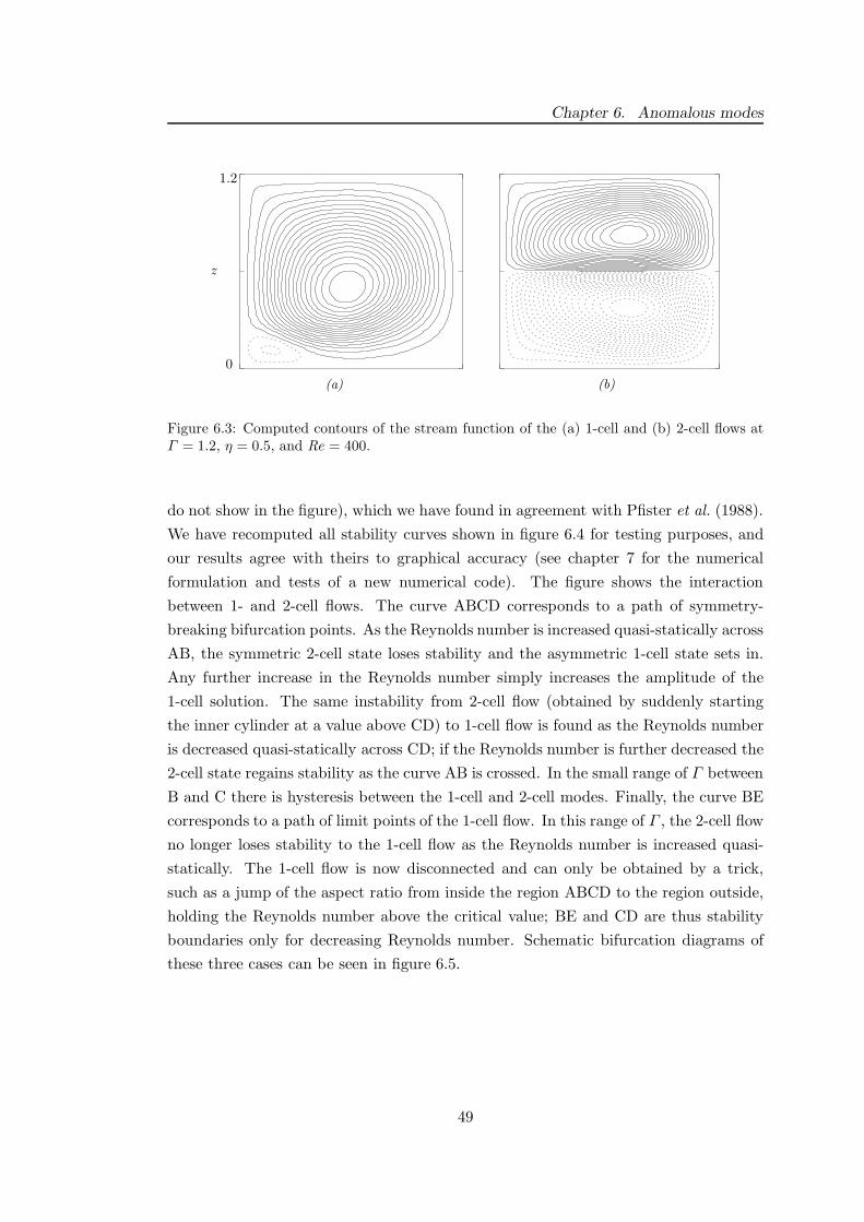
Chapter 6. Anomalous modes
0
z
1.2
(a)
(b)
Figure 6.3: Computed contours of the stream function of the (a) 1-cell and (b) 2-cell flows atΓ = 1.2, η = 0.5, and Re = 400.
do not show in the figure), which we have found in agreement with Pfister et al. (1988).
We have recomputed all stability curves shown in figure 6.4 for testing purposes, and
our results agree with theirs to graphical accuracy (see chapter 7 for the numerical
formulation and tests of a new numerical code). The figure shows the interaction
between 1- and 2-cell flows. The curve ABCD corresponds to a path of symmetry-
breaking bifurcation points. As the Reynolds number is increased quasi-statically across
AB, the symmetric 2-cell state loses stability and the asymmetric 1-cell state sets in.
Any further increase in the Reynolds number simply increases the amplitude of the
1-cell solution. The same instability from 2-cell flow (obtained by suddenly starting
the inner cylinder at a value above CD) to 1-cell flow is found as the Reynolds number
is decreased quasi-statically across CD; if the Reynolds number is further decreased the
2-cell state regains stability as the curve AB is crossed. In the small range of Γ between
B and C there is hysteresis between the 1-cell and 2-cell modes. Finally, the curve BE
corresponds to a path of limit points of the 1-cell flow. In this range of Γ , the 2-cell flow
no longer loses stability to the 1-cell flow as the Reynolds number is increased quasi-
statically. The 1-cell flow is now disconnected and can only be obtained by a trick,
such as a jump of the aspect ratio from inside the region ABCD to the region outside,
holding the Reynolds number above the critical value; BE and CD are thus stability
boundaries only for decreasing Reynolds number. Schematic bifurcation diagrams of
these three cases can be seen in figure 6.5.
49

Chapter 6. Anomalous modes
100
300
500
700
900
0.2 0.4 0.6 0.8 1.0 1.2 1.4 1.6
Rec
Γ
A
B C
D
E
120
160
200
1.20 1.28 1.36
BC
Figure 6.4: Critical steady Reynolds number Rec versus aspect ratio Γ for the transitionbetween 1- and 2-cell flows for η = 0.5. The arrows denote whether the boundaries can befound by a quasi-static increase (↑) or decrease (↓) of the Reynolds number. The inset is anenlargement of the hysteresis region.
50
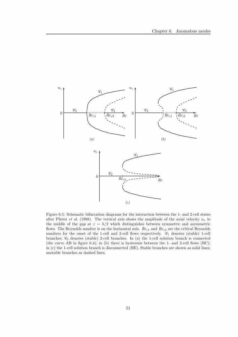
Chapter 6. Anomalous modes
0
uz
ReRec1 Rec2
C1
C2C2
(a)
0
uz
ReRec1 Rec2
C1
C2C2
(b)
0
uz
ReRec1
C1
C2
(c)
Figure 6.5: Schematic bifurcation diagrams for the interaction between the 1- and 2-cell statesafter Pfister et al. (1988). The vertical axis shows the amplitude of the axial velocity uz inthe middle of the gap at z = h/2 which distinguishes between symmetric and asymmetricflows. The Reynolds number is on the horizontal axis. Rec1 and Rec2 are the critical Reynoldsnumbers for the onset of the 1-cell and 2-cell flows respectively. C1 denotes (stable) 1-cellbranches; C2 denotes (stable) 2-cell branches. In (a) the 1-cell solution branch is connected(the curve AB in figure 6.4); in (b) there is hysteresis between the 1- and 2-cell flows (BC);in (c) the 1-cell solution branch is disconnected (BE). Stable branches are shown as solid lines;unstable branches as dashed lines.
51
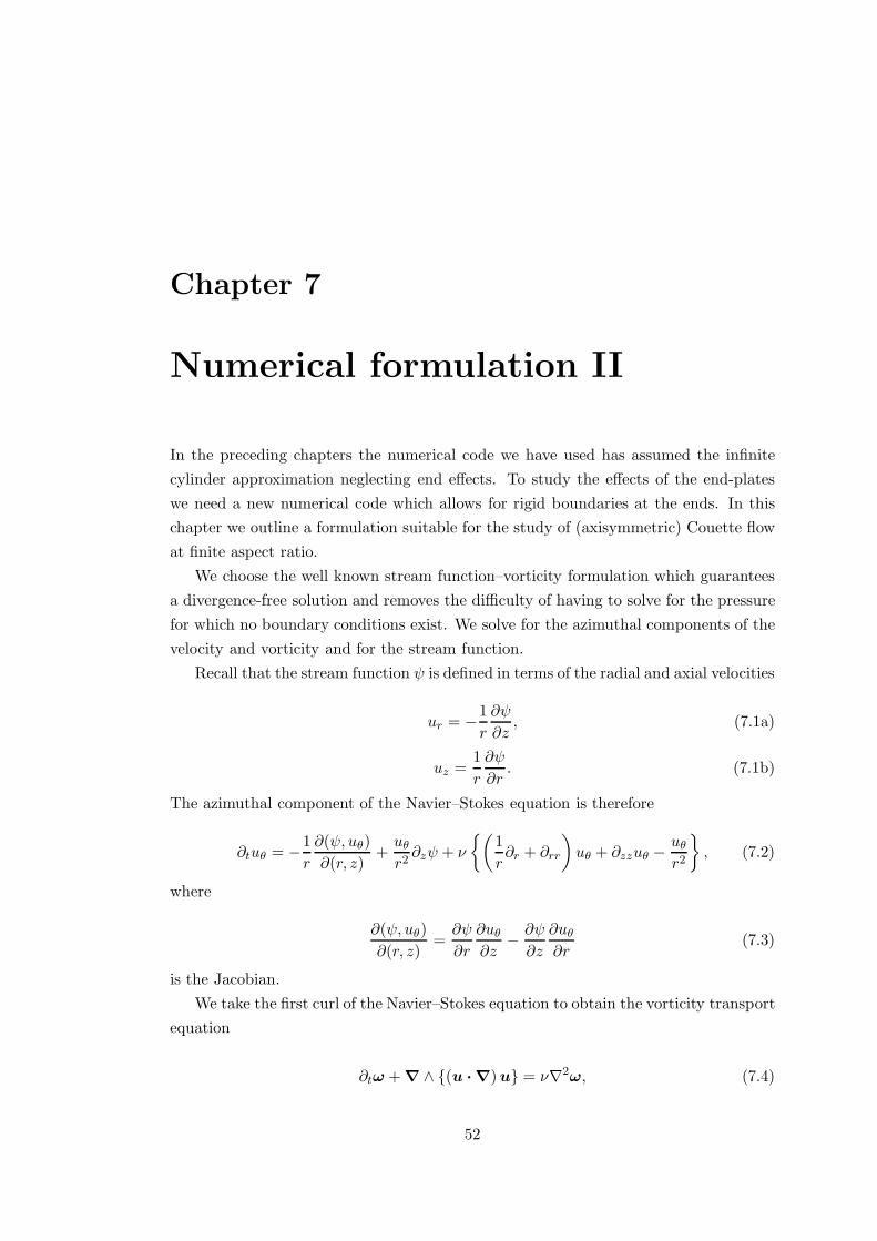
Chapter 7
Numerical formulation II
In the preceding chapters the numerical code we have used has assumed the infinite
cylinder approximation neglecting end effects. To study the effects of the end-plates
we need a new numerical code which allows for rigid boundaries at the ends. In this
chapter we outline a formulation suitable for the study of (axisymmetric) Couette flow
at finite aspect ratio.
We choose the well known stream function–vorticity formulation which guarantees
a divergence-free solution and removes the difficulty of having to solve for the pressure
for which no boundary conditions exist. We solve for the azimuthal components of the
velocity and vorticity and for the stream function.
Recall that the stream function ψ is defined in terms of the radial and axial velocities
ur = −1
r
∂ψ
∂z, (7.1a)
uz =1
r
∂ψ
∂r. (7.1b)
The azimuthal component of the Navier–Stokes equation is therefore
∂tuθ = −1
r
∂(ψ, uθ)
∂(r, z)+uθ
r2∂zψ + ν
(
1
r∂r + ∂rr
)
uθ + ∂zzuθ −uθ
r2
, (7.2)
where
∂(ψ, uθ)
∂(r, z)=∂ψ
∂r
∂uθ
∂z−∂ψ
∂z
∂uθ
∂r(7.3)
is the Jacobian.
We take the first curl of the Navier–Stokes equation to obtain the vorticity transport
equation
∂tω + ∇ ∧ (u · ∇) u = ν∇2ω, (7.4)
52
Chapter 7. Numerical formulation II
then taking the azimuthal component we have
∂tωθ =2uθ
r∂zuθ −
1
r
∂(ψ,ωθ)
∂(r, z)−ωθ
r2∂zψ + ν
(
1
r∂r + ∂rr
)
ωθ + ∂zzωθ −ωθ
r2
. (7.5)
Then using ω = ∇∧u we obtain a Poisson equation which allows us to determine the
stream function ψ from the azimuthal vorticity ωθ
ωθ = −1
r∂rrψ +
1
r2∂rψ −
1
r∂zzψ. (7.6)
Equations (7.4), (7.5), and (7.6) are made dimensionless with the transformations t→
δ2t/ν, z → δz, u → νu/δ, ω → νω/δ2, and ψ → νR2ψ, and with an adjusted radial
range r = R1 + δx with x ∈ [0, 1], which leads to the following dimensionless equations:
∂tuθ = ∂xxuθ +(1 − η)
s∂xuθ −
(1 − η)2
s2uθ + ∂zzuθ −
1
s
∂(ψ, uθ)
∂(x, z)+
(1 − η)
s2uθ∂zψ, (7.7)
∂tωθ = ∂xxωθ +(1 − η)
s∂xωθ −
(1 − η)2
s2ωθ + ∂zzωθ+
+2(1 − η)
suθ∂zuθ −
(1 − η)
s2ωθ∂zψ −
1
s
∂(ψ,ωθ)
∂(x, z), (7.8)
ωθ = −1
s∂xxψ +
(1 − η)
s2∂xψ −
1
s∂zzψ, (7.9)
where s = η + (1 − η)x.
Equations (7.7) and (7.8) are time stepped using a combination of second-order ac-
curate implicit Crank–Nicolson and explicit Adams–Bashforth methods. The Poisson
equation (7.9) for the stream function is solved using parallel ScaLAPACK linear alge-
bra routines (Blackford et al., 1997). The equations are discretised using second-order
centred finite differences.
With the time stepping and discretisation as above the equations can be written as
(1 − L1r − L1z)up+1θ = (1 + L1r + L1z) u
pθ + N1(u
pθ , u
p+1θ , ψp, ψp+1), (7.10)
(1 − L2r − L2z)ωp+1θ = (1 + L2r + L2z)ω
pθ + N2(u
pθ, u
p+1θ , ψp, ψp+1, ωp
θ , ωp+1θ ), (7.11)
53
Chapter 7. Numerical formulation II
ωp+1θ = (L3r + L3z)ψ
p+1, (7.12)
where Lir and Liz (i = 1, 2, 3) are linear operators that consist of r- and z-derivatives
respectively. N1 and N2 are nonlinear operators that operate on the variables in paren-
theses and p is the time index corresponding to time t = p∆t where ∆t is the time
step.
Equations (7.10)–(7.12) can be immediately written in matrix form; the left-hand
side matrices in the two diffusion equations are then banded due to the way in which
r- and z-derivatives appear in the linear operators. This is not so much of a problem
as there are many computational routines which are available for solving banded sys-
tems; nevertheless, storage requirements and execution times can be reduced by using
operator factorisation. This involves replacing the linear operator 1 − Lr − Lz with
(1 − Lr) (1 − Lz). The extra terms which arise in doing this have sizes less than or
equal to the time step error (∆t)2. We can now solve a tridiagonal system of equations,
firstly at each fixed position in z to give an intermediate solution, and then at each
fixed position in r to give the solution at the next time. The algorithm used to solve
the system then only requires the storage of the lower-diagonal, diagonal, and upper-
diagonal elements of the matrices, and, since the time step is fixed, these entries are
precomputed before the time stepping begins.
The Poisson equation for the stream function is solved using machine-optimised
parallel ScaLAPACK routines. This involves distributing the left-hand side (banded)
matrix over a process grid in block-column format (more details can be found in Black-
ford et al., 1997). A special low storage scheme is used to avoid storing the whole
matrix which is very sparse. An LU factorisation is performed on this distributed
matrix which is computed before the time stepping begins since the matrix does not
depend on time. The resulting factorisation is then used in a solver routine at each
time step.
The boundary conditions at the cylinder walls are the same as those detailed in
chapter 2. At the top and bottom ends, however, we implement the homotopy pa-
rameter of Schaeffer (1980), equation (6.1), to allow for a smooth transition between
stress-free and no-slip boundary conditions.
7.1 Numerical tests
Tests of the code have been performed in both the infinite and finite cylinder regimes.
In the infinite regime appropriate tests of the code are calculating linear growth rates,
nonlinear saturation and critical Reynolds numbers. The code has been tested against
the results of the code we use in the first part of this thesis (Willis & Barenghi, 2002a),
54

Chapter 7. Numerical formulation II
Nr ∆t σ % error
20 0.001 0.366853703 14.70670.0005 0.385106859 10.46290.0001 0.399699761 7.070060.00005 0.401520891 6.646650.00001 0.402941592 6.31633
40 0.0005 0.401071959 6.751020.0001 0.416512351 3.161140.00005 0.418439737 2.713020.00001 0.419990225 2.35254
60 0.0001 0.421393160 2.026360.00005 0.423365644 1.567750.00001 0.424886512 1.21415
80 0.0001 0.423321195 1.578090.00005 0.425300243 1.117960.00001 0.426899771 0.74607
100 0.00001 0.427742006 0.55025
Table 7.1: Growth rates σ and percentage errors at various mesh sizes and time steps. Thenumber of axial grid points is twice the number of radial grid points Nr. The radius ratio isη = 1/1.444, the axial wavenumber α = 3.13, the Reynolds number is Re = 80, and the growthrate as calculated by Barenghi (1991) using a spectral code is σ = 0.430108693.
which was in turn tested against known results as detailed in chapter 3. Table 7.1
compares our linear growth rates at a particular radius ratio and Reynolds number to
those of Barenghi (1991) who used a spectral code. This is a slightly unfair comparison
because a finite-difference code cannot be expected to attain the accuracy of a spectral
code without increasing the spatial resolution significantly; the figures do, however, give
an idea of how the accuracy scales with the time step and spatial resolution. Table 7.2
shows tests of nonlinear saturation by comparing the radial velocity at the outflow jet
r = (R1 + R2)/2, z = π/α against the results of Jones (1985a) for different spatial
resolutions and time steps. Even for low resolutions and large time steps the values are
well within 0.3% of his values.
In the finite cylinder regime an excellent test of the code is calculating critical
Reynolds numbers for the onset of the anomalous modes, and even more so for the
interaction of the 1- and 2- cell flows where end effects and the effects of the discon-
tinuity in the corners could be more apparent owing to the very short cylinders. In
the previous chapter we remarked that provided the mesh size is small enough in the
corners then the disturbance caused by the discontinuity is local to the corners. To test
this we increased the number of radial grid points from 80 to 160. We calculated the
critical Reynolds numbers of figure 6.4 at Γ = 0.25 on the curve AB, and at Γ = 0.97
on the curve CD, where the greatest inaccuracies lie in our code. The critical Reynolds
55

Chapter 7. Numerical formulation II
∆t Nr ur % error
Re = 72.4569
0.0001 20 4.22482008 0.2080940 4.22325946 0.2449680 4.22586180 0.18349
0.00001 20 4.23010942 0.0831640 4.22878916 0.1143480 4.23151505 0.04996
Re = 106.0660
0.0001 20 18.0064082 0.1998240 17.9732765 0.0154580 17.9667069 0.02111
0.00001 40 17.9780947 0.0422680 17.9716684 0.00650
Re = 150.0000
0.0001 20 33.7266734 0.1370940 33.6852613 0.0141480 33.6760509 0.01321
0.00001 40 33.6917453 0.0333980 33.6827541 0.00669
Table 7.2: Radial velocity at the outflow jet r = (R1 +R2)/2, z = π/α and percentage errors atthree different Reynolds numbers for different time steps and spatial resolutions Nr comparedto the values obtained by Jones (1985a) (4.23363, 17.9705, and 33.6805).
56

Chapter 7. Numerical formulation II
numbers are altered by 0.1% with the increase in the number of mesh points. There-
fore, in our numerical code we do not implement mesh refinement or give any special
treatment to the discontinuity in the corners. It is unfortunate that in the literature
critical Reynolds numbers are usually displayed as graphs, but are rarely tabulated.
Cliffe (1983) gives actual numerical values of critical Reynolds numbers at three differ-
ent aspect ratios Γ = 0.67, 1.00, and 1.187 (Γ = 0.67 and 1.187 were where the greatest
inaccuracies lay in his finite-element code) but his radius ratio is different to ours so
a direct comparison is not possible. Instead, we compare the critical values obtained
by our code to graphically estimated values of Pfister et al. (1988). At Γ = 0.67 (on
AB) our critical Reynolds number is 202.8, at Γ = 1.00 (on AB) it is 132.8, and at
Γ = 1.187 (on CD) it is 292.6. Pfister et al.’s corresponding (graphically estimated
∼ ±7%) critical values are 200, 132, and 295. Our results differ from theirs by ap-
proximately 1.4%, 0.6%, and 0.8% at the three values of Γ considered. A graphical
estimate (∼ ±2%) of the critical Reynolds number of Mullin et al. (2002) at Γ = 0.67
is Rec = 205 which differs from that of Pfister et al. by 2.5% and from ours by 1.1%.
The hysteresis region BC of figure 6.4 may be particularly sensitive to imperfections in
an experimental apparatus and also to inaccuracies in a numerical code. Pfister et al.
explicitly state the range of Γ for which the hysteresis is present and they determined
it to be 1.267 6 Γ 6 1.304; using our numerical code we have found the phenomenon to
exist for 1.267 6 Γ 6 1.294. The agreement is excellent. Some of our calculated critical
values for the interaction between the 1- and 2-cell modes can be seen in table C.3. As
explained in chapter 6, generating anomalous modes is a non-trivial task and so the
agreement of results in figures 6.2 and 6.4 with those already in the literature is an
indication that the code is capable.
57
Chapter 8
Axisymmetric modulated
Couette flow between finite
cylinders
The aim of the work in this chapter is two-fold. Firstly, we want to determine whether
or not, in the case of a temporally modulated flow, the presence of the ends and
the resulting Ekman circulation can prevent the occurrence of the reversing or non-
reversing flows found in chapters 4 and 5. Secondly, we want to explore the very small
aspect ratio regime. In this case we examine the effect of a temporal modulation on
the selection of the 1- and 2-cell flow structures that have been observed in the steady
case. Essentially we want to determine whether the transition from RTVF to the newly
discovered NRTVF depends on the cylinders’ finite height in an actual experimental
apparatus.
In the infinite cylinder approximation, and in relatively long cylinders, the vortices
which form are true Taylor vortices in the sense that each pair of vortices has a fixed
wavelength over (most of) the length of the cylinders. Strictly speaking, however, once
the cylinders become shorter it is no longer appropriate to describe the formation of
Taylor vortices due to the presence of the Ekman circulation, which can cause the
wavelength of a pair of vortices to vary along the length of the cylinders; instead we
describe the formation of cells. Because of the difficulty in knowing exactly when we
have the formation of Taylor vortices or the formation of cells we use the two words
‘vortices’ and ‘cells’ interchangeably throughout this chapter.
58
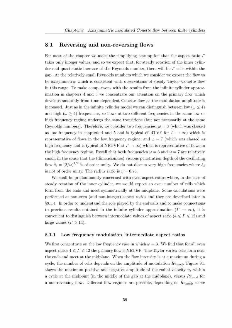
Chapter 8. Axisymmetric modulated Couette flow between finite cylinders
8.1 Reversing and non-reversing flows
For most of the chapter we make the simplifying assumption that the aspect ratio Γ
takes only integer values, and so we expect that, for steady rotation of the inner cylin-
der and quasi-static increase of the Reynolds number, there will be Γ cells within the
gap. At the relatively small Reynolds numbers which we consider we expect the flow to
be axisymmetric which is consistent with observations of steady Taylor–Couette flow
in this range. To make comparisons with the results from the infinite cylinder approx-
imation in chapters 4 and 5 we concentrate our attention on the primary flow which
develops smoothly from time-dependent Couette flow as the modulation amplitude is
increased. Just as in the infinite cylinder model we can distinguish between low (ω > 4)
and high (ω ? 4) frequencies, so flows at two different frequencies in the same low or
high frequency regime undergo the same transitions (but not necessarily at the same
Reynolds numbers). Therefore, we consider two frequencies, ω = 3 (which was classed
as low frequency in chapters 4 and 5 and is typical of RTVF for Γ → ∞) which is
representative of flows in the low frequency regime, and ω = 7 (which was classed as
high frequency and is typical of NRTVF at Γ → ∞) which is representative of flows in
the high frequency regime. Recall that both frequencies ω = 3 and ω = 7 are relatively
small, in the sense that the (dimensionless) viscous penetration depth of the oscillating
flow δs = (2/ω)1/2 is of order unity. We do not discuss very high frequencies where δs
is not of order unity. The radius ratio is η = 0.75.
We shall be predominantly concerned with even aspect ratios where, in the case of
steady rotation of the inner cylinder, we would expect an even number of cells which
form from the ends and meet symmetrically at the midplane. Some calculations were
performed at non-even (and non-integer) aspect ratios and they are described later in
§8.1.4. In order to understand the role played by the endwalls and to make connections
to previous results obtained in the infinite cylinder approximation (Γ → ∞), it is
convenient to distinguish between intermediate values of aspect ratio (4 6 Γ 6 12) and
large values (Γ > 14).
8.1.1 Low frequency modulation, intermediate aspect ratios
We first concentrate on the low frequency case in which ω = 3. We find that for all even
aspect ratios 4 6 Γ 6 12 the primary flow is NRTVF. The Taylor vortex cells form near
the ends and meet at the midplane. When the flow intensity is at a maximum during a
cycle, the number of cells depends on the amplitude of modulation Remod. Figure 8.1
shows the maximum positive and negative amplitude of the radial velocity ur within
a cycle at the midpoint (in the middle of the gap at the midplane), versus Remod for
a non-reversing flow. Different flow regimes are possible, depending on Remod, so we
59

Chapter 8. Axisymmetric modulated Couette flow between finite cylinders
−10
0
10
20
30
40
100 120 140 160 180 200
amp(u
r)
Remod
Figure 8.1: Maximum positive amplitude (solid) and maximum negative amplitude (dashed)of the radial velocity ur (at the midpoint r = 1 + η/2(1− η) and z = Γ/2) versus amplitude ofmodulation Remod for NRTVF at η = 0.75, Γ = 8, and ω = 3.
distinguish between small, intermediate, and large amplitudes of modulation.
Small amplitude of modulation
To illustrate this regime we choose Remod = 140 at Γ = 8. Figure 8.2 shows the
radial velocity ur at the midpoint versus time over a cycle for NRTVF. The period of
the forcing is T = 2π/ω and the flow responds synchronously with a period of T/2.
This is in agreement with the results of chapters 4 and 5 under the infinite cylinder
approximation.
The primary flow developing from oscillating azimuthal flow is a non-reversing flow
with an inflow at the midplane. When the cells have fully formed there are Γ = 8
cells within the gap, inflows near the endwalls, and, since Γ/2 = 4 is even, an inflow
at the midplane. Figure 8.4 shows computed contour plots of the stream function for
NRTVF at various times over half a cycle with parameters as in figure 8.1 and for
Remod = 140. For the sake of graphical clarity, we do not plot the stream function
over the entire range 0 6 z 6 Γ = 8. The reason for this is that the cells close to the
endwalls are always visible even at very low rotation rates, so when the radial velocity
at the midplane is very small it may be much larger near the endwalls. Consequently,
using the same number of contour levels over the whole length of the cylinders would
either hide the structure close to the midplane as shown in figure 8.3(a) or make the
60
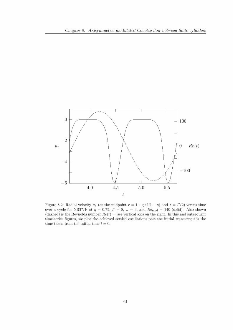
Chapter 8. Axisymmetric modulated Couette flow between finite cylinders
−6
−4
−2
0
4.0 4.5 5.0 5.5
−100
0
100
ur Re(t)
t
Figure 8.2: Radial velocity ur (at the midpoint r = 1 + η/2(1 − η) and z = Γ/2) versus timeover a cycle for NRTVF at η = 0.75, Γ = 8, ω = 3, and Remod = 140 (solid). Also shown(dashed) is the Reynolds number Re(t) — see vertical axis on the right. In this and subsequenttime-series figures, we plot the achieved settled oscillations past the initial transient; t is thetime taken from the initial time t = 0.
61
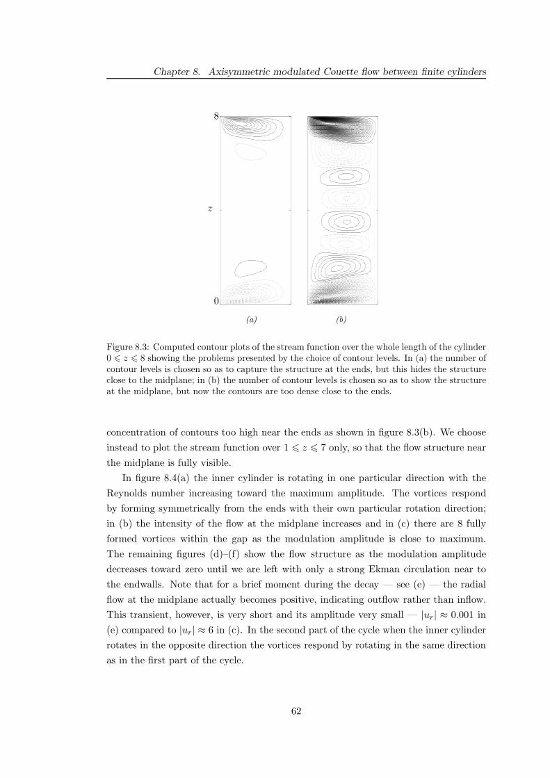
Chapter 8. Axisymmetric modulated Couette flow between finite cylinders
0
z
8
(a)
(b)
Figure 8.3: Computed contour plots of the stream function over the whole length of the cylinder0 6 z 6 8 showing the problems presented by the choice of contour levels. In (a) the number ofcontour levels is chosen so as to capture the structure at the ends, but this hides the structureclose to the midplane; in (b) the number of contour levels is chosen so as to show the structureat the midplane, but now the contours are too dense close to the ends.
concentration of contours too high near the ends as shown in figure 8.3(b). We choose
instead to plot the stream function over 1 6 z 6 7 only, so that the flow structure near
the midplane is fully visible.
In figure 8.4(a) the inner cylinder is rotating in one particular direction with the
Reynolds number increasing toward the maximum amplitude. The vortices respond
by forming symmetrically from the ends with their own particular rotation direction;
in (b) the intensity of the flow at the midplane increases and in (c) there are 8 fully
formed vortices within the gap as the modulation amplitude is close to maximum.
The remaining figures (d)–(f) show the flow structure as the modulation amplitude
decreases toward zero until we are left with only a strong Ekman circulation near to
the endwalls. Note that for a brief moment during the decay — see (e) — the radial
flow at the midplane actually becomes positive, indicating outflow rather than inflow.
This transient, however, is very short and its amplitude very small — |ur| ≈ 0.001 in
(e) compared to |ur| ≈ 6 in (c). In the second part of the cycle when the inner cylinder
rotates in the opposite direction the vortices respond by rotating in the same direction
as in the first part of the cycle.
62
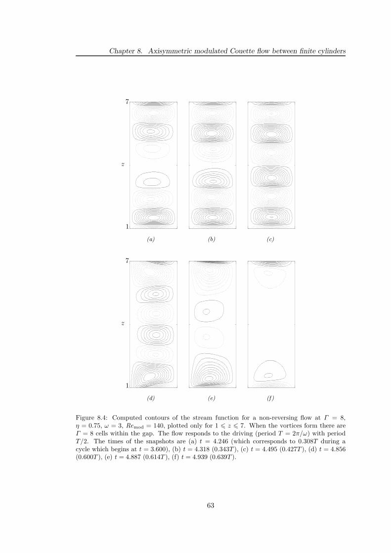
Chapter 8. Axisymmetric modulated Couette flow between finite cylinders
1
z
7
(a)
(b)
(c)
1
z
7
(d)
(e)
(f)
Figure 8.4: Computed contours of the stream function for a non-reversing flow at Γ = 8,η = 0.75, ω = 3, Remod = 140, plotted only for 1 6 z 6 7. When the vortices form there areΓ = 8 cells within the gap. The flow responds to the driving (period T = 2π/ω) with periodT/2. The times of the snapshots are (a) t = 4.246 (which corresponds to 0.308T during acycle which begins at t = 3.600), (b) t = 4.318 (0.343T ), (c) t = 4.495 (0.427T ), (d) t = 4.856(0.600T ), (e) t = 4.887 (0.614T ), (f) t = 4.939 (0.639T ).
63
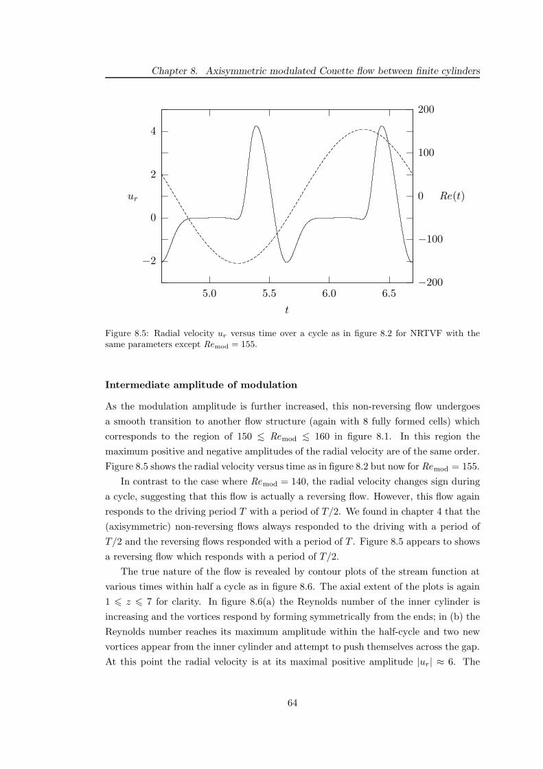
Chapter 8. Axisymmetric modulated Couette flow between finite cylinders
−2
0
2
4
5.0 5.5 6.0 6.5−200
−100
0
100
200
ur Re(t)
t
Figure 8.5: Radial velocity ur versus time over a cycle as in figure 8.2 for NRTVF with thesame parameters except Remod = 155.
Intermediate amplitude of modulation
As the modulation amplitude is further increased, this non-reversing flow undergoes
a smooth transition to another flow structure (again with 8 fully formed cells) which
corresponds to the region of 150 > Remod > 160 in figure 8.1. In this region the
maximum positive and negative amplitudes of the radial velocity are of the same order.
Figure 8.5 shows the radial velocity versus time as in figure 8.2 but now for Remod = 155.
In contrast to the case where Remod = 140, the radial velocity changes sign during
a cycle, suggesting that this flow is actually a reversing flow. However, this flow again
responds to the driving period T with a period of T/2. We found in chapter 4 that the
(axisymmetric) non-reversing flows always responded to the driving with a period of
T/2 and the reversing flows responded with a period of T . Figure 8.5 appears to shows
a reversing flow which responds with a period of T/2.
The true nature of the flow is revealed by contour plots of the stream function at
various times within half a cycle as in figure 8.6. The axial extent of the plots is again
1 6 z 6 7 for clarity. In figure 8.6(a) the Reynolds number of the inner cylinder is
increasing and the vortices respond by forming symmetrically from the ends; in (b) the
Reynolds number reaches its maximum amplitude within the half-cycle and two new
vortices appear from the inner cylinder and attempt to push themselves across the gap.
At this point the radial velocity is at its maximal positive amplitude |ur| ≈ 6. The
64
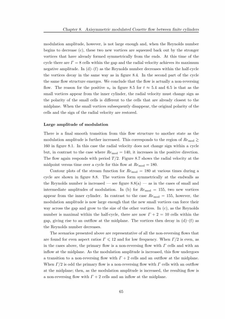
Chapter 8. Axisymmetric modulated Couette flow between finite cylinders
modulation amplitude, however, is not large enough and, when the Reynolds number
begins to decrease (c), these two new vortices are squeezed back out by the stronger
vortices that have already formed symmetrically from the ends. At this time of the
cycle there are Γ = 8 cells within the gap and the radial velocity achieves its maximum
negative amplitude. In (d)–(f) as the Reynolds number decreases within the half-cycle
the vortices decay in the same way as in figure 8.4. In the second part of the cycle
the same flow structure emerges. We conclude that the flow is actually a non-reversing
flow. The reason for the positive ur in figure 8.5 for t ≈ 5.4 and 6.5 is that as the
small vortices appear from the inner cylinder, the radial velocity must change sign as
the polarity of the small cells is different to the cells that are already closest to the
midplane. When the small vortices subsequently disappear, the original polarity of the
cells and the sign of the radial velocity are restored.
Large amplitude of modulation
There is a final smooth transition from this flow structure to another state as the
modulation amplitude is further increased. This corresponds to the region of Remod ?
160 in figure 8.1. In this case the radial velocity does not change sign within a cycle
but, in contrast to the case where Remod = 140, it increases in the positive direction.
The flow again responds with period T/2. Figure 8.7 shows the radial velocity at the
midpoint versus time over a cycle for this flow at Remod = 180.
Contour plots of the stream function for Remod = 180 at various times during a
cycle are shown in figure 8.8. The vortices form symmetrically at the endwalls as
the Reynolds number is increased — see figure 8.8(a) — as in the cases of small and
intermediate amplitudes of modulation. In (b) for Remod = 155, two new vortices
appear from the inner cylinder. In contrast to the case Remod = 155, however, the
modulation amplitude is now large enough that the new small vortices can force their
way across the gap and grow to the size of the other vortices. In (c), as the Reynolds
number is maximal within the half-cycle, there are now Γ + 2 = 10 cells within the
gap, giving rise to an outflow at the midplane. The vortices then decay in (d)–(f) as
the Reynolds number decreases.
The scenarios presented above are representative of all the non-reversing flows that
are found for even aspect ratios Γ 6 12 and for low frequency. When Γ/2 is even, as
in the cases above, the primary flow is a non-reversing flow with Γ cells and with an
inflow at the midplane. As the modulation amplitude is increased, this flow undergoes
a transition to a non-reversing flow with Γ + 2 cells and an outflow at the midplane.
When Γ/2 is odd the primary flow is a non-reversing flow with Γ cells with an outflow
at the midplane; then, as the modulation amplitude is increased, the resulting flow is
a non-reversing flow with Γ + 2 cells and an inflow at the midplane.
65

Chapter 8. Axisymmetric modulated Couette flow between finite cylinders
1
z
7
(a)
(b)
(c)
1
z
7
(d)
(e)
(f)
Figure 8.6: Computed contours of the stream function for a non-reversing flow at Γ = 8,η = 0.75, ω = 3, Remod = 155, and for 1 6 Γ 6 7. When the vortices form there areΓ = 8 cells within the gap. The flow responds to the driving with period T/2. The times ofthe snapshots are (a) t = 5.254 (which corresponds to 0.312T during a cycle which begins att = 4.600), (b) t = 5.410 (0.387T ), (c) t = 5.629 (0.491T ), (d) t = 5.906 (0.624T ), (e) t = 5.938(0.639T ), (f) t = 6.042 (0.689T ).
66
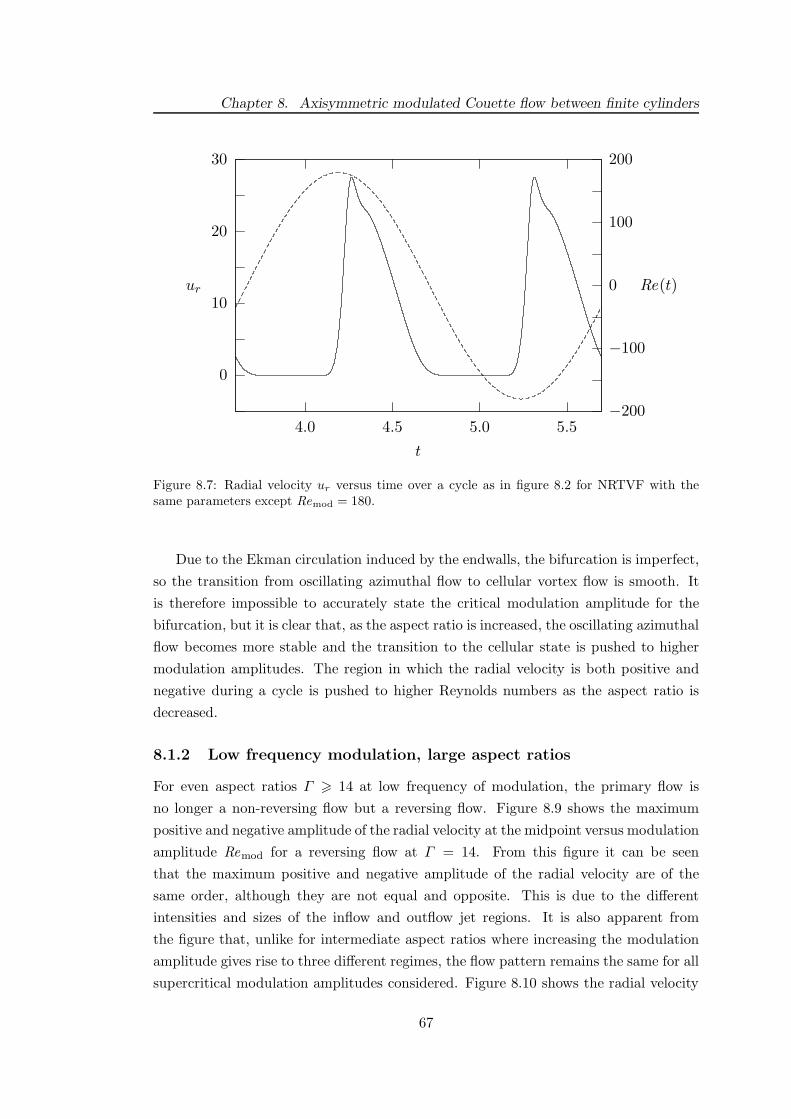
Chapter 8. Axisymmetric modulated Couette flow between finite cylinders
0
10
20
30
4.0 4.5 5.0 5.5−200
−100
0
100
200
ur Re(t)
t
Figure 8.7: Radial velocity ur versus time over a cycle as in figure 8.2 for NRTVF with thesame parameters except Remod = 180.
Due to the Ekman circulation induced by the endwalls, the bifurcation is imperfect,
so the transition from oscillating azimuthal flow to cellular vortex flow is smooth. It
is therefore impossible to accurately state the critical modulation amplitude for the
bifurcation, but it is clear that, as the aspect ratio is increased, the oscillating azimuthal
flow becomes more stable and the transition to the cellular state is pushed to higher
modulation amplitudes. The region in which the radial velocity is both positive and
negative during a cycle is pushed to higher Reynolds numbers as the aspect ratio is
decreased.
8.1.2 Low frequency modulation, large aspect ratios
For even aspect ratios Γ > 14 at low frequency of modulation, the primary flow is
no longer a non-reversing flow but a reversing flow. Figure 8.9 shows the maximum
positive and negative amplitude of the radial velocity at the midpoint versus modulation
amplitude Remod for a reversing flow at Γ = 14. From this figure it can be seen
that the maximum positive and negative amplitude of the radial velocity are of the
same order, although they are not equal and opposite. This is due to the different
intensities and sizes of the inflow and outflow jet regions. It is also apparent from
the figure that, unlike for intermediate aspect ratios where increasing the modulation
amplitude gives rise to three different regimes, the flow pattern remains the same for all
supercritical modulation amplitudes considered. Figure 8.10 shows the radial velocity
67

Chapter 8. Axisymmetric modulated Couette flow between finite cylinders
1
z
7
(a)
(b)
(c)
1
z
7
(d)
(e)
(f)
Figure 8.8: Computed contours of the stream function for a non-reversing flow at Γ = 8,η = 0.75, ω = 3, Remod = 180, and for 1 6 Γ 6 7. When the vortices form there areΓ + 2 = 10 cells within the gap. The flow responds to the driving with period T/2. The timesof the snapshots are (a) t = 4.156 (which corresponds to 0.256T during a cycle which begins att = 3.620), (b) t = 4.198 (0.276T ), (c) t = 4.281 (0.316T ), (d) t = 4.777 (0.552T ), (e) t = 4.870(0.597T ), (f) t = 4.933 (0.627T ).
68

Chapter 8. Axisymmetric modulated Couette flow between finite cylinders
−20
0
20
40
100 120 140 160 180
amp(u
r)
Remod
Figure 8.9: Maximum positive amplitude (solid) and maximum negative amplitude (dashed)of the radial velocity ur (measured at r = 1 + η/2(1 − η) and z = Γ/2) versus amplitude ofmodulation Remod for RTVF at η = 0.75, Γ = 14, and ω = 3.
at the midpoint versus time over a full cycle: note that ur changes sign with Re(t).
The number of cells that fill the gap now depends on the Reynolds number within
a cycle. For the first part of the cycle, when the Reynolds number is positive, there
are Γ = 14 cells within the gap; for the second part of the cycle, when the Reynolds
number is negative, there are Γ +2 = 16 cells within the gap. In the most general case
it would be possible for there to be Γ + 2 cells when the Reynolds number is positive
and Γ cells when the Reynolds number is negative. This is again just a matter of the
sign of the initial condition. As for the case of infinite cylinders (chapters 4 and 5),
there is a smooth transition between these two states as the nodal line crosses the
gap. The key difference between the case of finite but large aspect ratio and the limit
Γ → ∞ is that, for finite Γ , not all the vortices reverse their rotation direction. We
find that the cells closest to the endwalls always rotate in the same direction during
a cycle, leaving a reversing flow in a section away from the endwalls. Two new cells
appear symmetrically about the midplane at the boundary between the reversing and
non-reversing cells. This is why there are Γ cells for the first part of the cycle and
Γ + 2 cells for the second part.
We illustrate the low frequency, large aspect ratio regime with Remod = 170 which
is representative of the flows found for Remod ? 140. Figure 8.11 shows contours of
the stream function for a reversing flow at Γ = 14 and Remod = 170 at two different
69
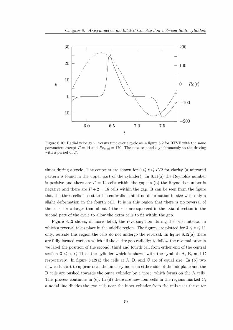
Chapter 8. Axisymmetric modulated Couette flow between finite cylinders
−10
0
10
20
30
6.0 6.5 7.0 7.5−200
−100
0
100
200
ur Re(t)
t
Figure 8.10: Radial velocity ur versus time over a cycle as in figure 8.2 for RTVF with the sameparameters except Γ = 14 and Remod = 170. The flow responds synchronously to the drivingwith a period of T .
times during a cycle. The contours are shown for 0 6 z 6 Γ/2 for clarity (a mirrored
pattern is found in the upper part of the cylinder). In 8.11(a) the Reynolds number
is positive and there are Γ = 14 cells within the gap; in (b) the Reynolds number is
negative and there are Γ + 2 = 16 cells within the gap. It can be seen from the figure
that the three cells closest to the endwalls exhibit no deformation in size with only a
slight deformation in the fourth cell. It is in this region that there is no reversal of
the cells; for z larger than about 4 the cells are squeezed in the axial direction in the
second part of the cycle to allow the extra cells to fit within the gap.
Figure 8.12 shows, in more detail, the reversing flow during the brief interval in
which a reversal takes place in the middle region. The figures are plotted for 3 6 z 6 11
only; outside this region the cells do not undergo the reversal. In figure 8.12(a) there
are fully formed vortices which fill the entire gap radially; to follow the reversal process
we label the position of the second, third and fourth cell from either end of the central
section 3 6 z 6 11 of the cylinder which is shown with the symbols A, B, and C
respectively. In figure 8.12(a) the cells at A, B, and C are of equal size. In (b) two
new cells start to appear near the inner cylinder on either side of the midplane and the
B cells are pushed towards the outer cylinder by a ‘nose’ which forms on the A cells.
This process continues in (c). In (d) there are now four cells in the regions marked C;
a nodal line divides the two cells near the inner cylinder from the cells near the outer
70
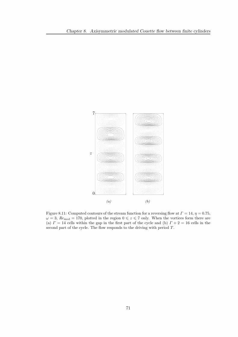
Chapter 8. Axisymmetric modulated Couette flow between finite cylinders
0
z
7
(a)
(b)
Figure 8.11: Computed contours of the stream function for a reversing flow at Γ = 14, η = 0.75,ω = 3, Remod = 170, plotted in the region 0 6 z 6 7 only. When the vortices form there are(a) Γ = 14 cells within the gap in the first part of the cycle and (b) Γ + 2 = 16 cells in thesecond part of the cycle. The flow responds to the driving with period T .
71

Chapter 8. Axisymmetric modulated Couette flow between finite cylinders
cylinder, exactly as in our previous calculations with the infinite cylinder model. The
nodal line moves quickly across the gap; the cells at B are pushed radially out by the
growing cells at A. Finally, in (f) there are now fully formed vortices which extend
across the gap with opposite polarity to those in (a).
The reversal process takes place in a fraction of a diffusion time and the time scale
on which it occurs is comparable to the time scale based on the modulation amplitude
Ωa of the inner cylinder. The relation between the time based on the diffusion time
scale tdiff and the time based on the modulation amplitude of the inner cylinder tmod
is tmod = Remod(1 − η)tdiff/η.
As the aspect ratio is increased, the number of vortices undergoing a complete
reversal increases; the number of vortices close to the ends which do not undergo a
reversal remains roughly constant at about 3–5. This is true for all aspect ratios up to
the largest we examined at Γ = 40, and at this aspect ratio most of the vortices within
the gap are free from the influence of the Ekman circulation.
8.1.3 High frequency of modulation
At the higher frequency of ω = 7 there is no evidence of any reversing flow for all aspect
ratios considered 4 6 Γ 6 40. This is in agreement with the infinite cylinder model
where only non-reversing flows were found at higher frequencies. The only interesting
feature of the high-frequency case is the number of cells that are formed when the
Reynolds number is supercritical. For even aspect ratios 4 6 Γ 6 8 the primary flow
is a non-reversing flow with Γ cells but for Γ > 10 the primary flow is a non-reversing
flow with Γ + 2 cells. As in the low frequency case, these non-reversing flows respond
to the driving with period T/2.
In the high frequency case it is straightforward to find a secondary disconnected
flow. To begin with, a flow on the primary branch is found with modulation amplitude
+Remod; for 4 6 Γ 6 8 this flow has Γ cells, for Γ > 10 it has Γ +2 cells. Then, within
the cycle, the sign of the modulation amplitude is instantaneously switched to −Remod.
This corresponds to an instantaneous change of rotation direction of the inner cylinder.
The resulting flow is on the disconnected branch of the bifurcation and for 4 6 Γ 6 8
this flow has Γ + 2 cells, whereas for Γ > 10 it has Γ + 4 cells. All these flows respond
to the driving with period T/2.
8.1.4 Non-integer, non-even aspect ratios
Some calculations have been done to determine the transition between flows as the
aspect ratio is increased but the modulation amplitude is fixed.
For intermediate aspect ratios and low frequencies the flow patterns observed are
qualitatively similar to those when fixing the aspect ratio and varying the modulation
72

Chapter 8. Axisymmetric modulated Couette flow between finite cylinders
3
z
11
A
A
B
B
C
C
(a)
A
A
B
B
C
C
(b)
A
A
B
B
C
C
(c)
3
z
11
A
A
B
B
C
C
(d)
A
A
C
C
(e)
A
A
C
C
(f)
Figure 8.12: Computed contours of the stream function for a reversing flow at Γ = 14, η = 0.75,ω = 3, Remod = 170, plotted in 3 6 z 6 11 only as the reversal process takes place. The flowresponds to the driving with period T . The times of the snapshots are (a) t = 6.916 (whichcorresponds to 0.581T during a cycle which begins at t = 5.700), (b) t = 6.956 (0.600T ), (c)t = 6.962 (0.603T ), (d) t = 6.966 (0.604T ), (e) t = 6.970 (0.606T ), (f) t = 7.006 (0.624T ). Notehow the B cells are pushed radially out until they disappear.
73
Chapter 8. Axisymmetric modulated Couette flow between finite cylinders
amplitude as in figures 8.4, 8.6 and 8.8. If we let Γ1 and Γ2 > Γ1 be two consecutive
even aspect ratios (and for not too large modulation amplitude) then when Γ = Γ1 the
primary flow consists of Γ1 cells and when Γ = Γ2 the primary flow consists of Γ2 cells.
These flows are non-reversing flows. As the aspect ratio is increased from Γ1 to Γ2 two
new cells start to appear from the inner cylinder just as in the case of intermediate
amplitude of modulation with fixed aspect ratio (figure 8.6). When the aspect ratio is
not large enough these two new cells are squeezed back out by the existing cells leaving
a flow with Γ1 cells; when the aspect ratio is larger, however, these two new cells are
able to extend across the gap and grow to the size of the existing vortices leaving a flow
with Γ2 cells (figure 8.8). This is a smooth process as the aspect ratio is increased and
there is no definite aspect ratio at which the two new cells appear. The same process
occurs for higher modulation amplitudes where the flow consists of Γ + 2 cells.
For larger aspect ratios and low frequencies a slightly different transition takes place
as the aspect ratio is increased from Γ1 to Γ2. When Γ = Γ1 the flow is reversing with
Γ1 cells in the first part of the cycle and Γ1 +2 cells in the second part of the cycle. As
the aspect ratio is increased toward Γ2 the flow is still reversing but now has Γ2 cells in
the first part of the cycle and Γ2+2 cells in the second part of the cycle. Describing the
transition as the aspect ratio is increased is most easily undertaken using an example
and with reference to figure 8.13 where Γ = 15, Remod = 150, and ω = 3. Let Γ1 = 14
and Γ2 = 16, then when Γ = 14 there are 14 cells in the first part of the cycle and
16 in the second part of the cycle; when Γ = 16 there are 16 cells in the first part of
the cycle and 18 in the second part of the cycle. If the aspect ratio is increased but is
not large enough then there is still an oscillation of 14 and 16 cells within the cycle. If
the aspect ratio is further increased 18 cells try to fit in the gap creating an oscillation
between 16 and 18 cells. This attempt is seen as two new cells appearing from the
inner cylinder as in figure 8.13(a) but not at the midplane — the two new cells try
to fit in two cells away from the midplane and they are incredibly compressed in the
axial direction. Figure 8.13(b) shows the two new cells pushing further across the gap.
If the aspect ratio is still not large enough, however, these two new cells are squeezed
out (figure 8.13(c)) and the two cells that were either side of them coalesce to form a
new cell leaving 14 cells in the gap (figures 8.13(d)– (f)). Once the aspect ratio is large
enough the two new cells are robust enough to survive and the flow does indeed show
an oscillation between 16 and 18 cells. Just as for intermediate aspect ratios this is
also a smooth process and there is no definite aspect ratio where the oscillation can be
seen to be between 16 and 18 cells rather than between 14 and 16.
The picture is not so clear for aspect ratios in the range 12 < Γ < 14. In this range
of aspect ratios it is very difficult to obtain critical modulation amplitudes or aspect
ratios for transitions between reversing and non-reversing flows and also for transitions
74

Chapter 8. Axisymmetric modulated Couette flow between finite cylinders
3
z
12
(a)
(b)
(c)
3
z
12
(d)
(e)
(f)
Figure 8.13: Computed contours of the stream function showing the appearance of extra cells inthe second part of the cycle of a reversing flow with non-even aspect ratio Γ = 15, Remod = 150,and ω = 3. The appearance of the extra cells means that 18 cells try to fit in the gap, but theaspect ratio is not large enough and they are squeezed out leaving 14 cells. The flow respondsto the driving with period T . The times of the snapshots are (a) t = 12.812 (which correspondsto 0.497T during a cycle which begins at t = 11.771), (b) t = 12.874 (0.527T ), (c) t = 12.979(0.577T ), (d) t = 13.000 (0.587T ), (d) t = 13.104 (0.636T ), (f) t = 13.209 (0.687T ).
75
Chapter 8. Axisymmetric modulated Couette flow between finite cylinders
of flows with different numbers of cells. The main reason for this is that there is now
competition between the reversing and non-reversing flows. Some progress has been
made, however, in determining a general picture of the transitions. For most of the
range the primary flow is a non-reversing flow which initially has 12 cells but which
undergoes a smooth transition to 14 cells as the modulation amplitude is increased (just
as in the intermediate aspect ratio regime Γ 6 12). However, a sufficient discontinuous
jump in the modulation amplitude close to the critical region for the onset of the
primary flow causes the flow to become a reversing flow with an oscillation between
14 and 16 cells (just as in the large aspect ratio regime Γ > 14). For example, at
Γ = 13 the non-reversing flow is the primary flow at Remod ≈ 140. If the modulation
amplitude is increased suddenly to 147 the flow remains as a non-reversing flow; if the
modulation amplitude is increased suddenly from 140 to 148, however, the flow is a
reversing flow.
When the frequency is higher, the reversing flows no longer exist and the transitions
between non-reversing flows as the aspect ratio is increased are the same as for the low
frequency case.
8.2 Very small aspect ratio
Now we turn our attention to the case where the height of the cylinders is of the order
of the gap width (and Γ is no longer restricted to being an integer). In this regime
reversing and non-reversing flows do not exist and we no longer discuss transitions
between them. For the rest of this chapter we consider a radius ratio of η = 0.5,
and figure 6.4 shows the region of parameter space examined for steady flows which is
relevant to our investigation of modulated flows. (See chapter 6 for a detailed discussion
of the steady flows in this regime.)
If the inner cylinder does not rotate at constant angular velocity but is modulated
as in equation (1.2), a direct comparison with figure 6.4 is not possible. The reason
is that there is no equivalent to a sudden start of the cylinder — the time-dependent
Reynolds number changes smoothly during a cycle. We should not expect to be able to
find boundaries such as CD or BE, which are realised by sudden jumps in the Reynolds
number above the boundaries in the steady case.
At subcritical modulation amplitudes the basic flow is a symmetric 2-cell flow,
similar to the steady case as shown in figure 6.3(b). The only effect of the modulation
is to cause a slight deformation of the cells and to make the vortex cores shift slightly
during the cycle. The midplane region is always an outflow (the cells do not switch
sign).
As in the steady case, the bifurcation from the oscillatory 2-cell flow is to an asym-
76

Chapter 8. Axisymmetric modulated Couette flow between finite cylinders
0
z
1
(a)
(b)
(c)
0
z
1
(d)
(e)
(f)
Figure 8.14: Computed contours of the stream function for the oscillation between 1- and2-cell flows at Γ = 1, η = 0.5, ω = 4, Remod = 400. The times of the snapshots are (a)t = 17.059 (which corresponds to 0.006T during a cycle which begins at t = 17.050), (b)t = 17.355 (0.194T ), (c) t = 17.433 (0.244T ), (d) t = 17.612 (0.358T ), (e) t = 17.729 (0.432T ),(f) t = 17.807 (0.482T ).
metric state with non-zero axial velocity at the midplane. For various modulation
frequencies ranging from ω = 3 to ω = 50 we have found that only when the modula-
tion amplitude is large enough can a definite asymmetric flow pattern be recognised;
an example is shown in figure 8.14, where Γ = 1, ω = 4, and Remod = 400.
Over the period T/2 (where T is the period of the forcing) an oscillation between
the two states shown in figure 6.3 occurs. The flow responds to the driving with period
T/2. When the time-dependent Reynolds number is less than the critical modulation
amplitude the flow is a symmetric 2-cell state, but when it is greater than critical the
flow is an asymmetric 1-cell state, with a smooth transition between the two states.
As the modulation frequency is increased significantly, the flow has less time to os-
cillate fully between the symmetric and asymmetric states, and so for larger frequencies
the flow remains in an asymmetric state as in figure 6.3(a), with slight deformations of
the cells and movement of the vortex cores.
Although it is not possible to accurately calculate the critical modulation amplitude
of the onset of this asymmetry, it is clear that the modulation has a stabilising effect
77

Chapter 8. Axisymmetric modulated Couette flow between finite cylinders
and so the symmetry-breaking bifurcation occurs at larger Reynolds numbers than in
the steady case.
We have also found that, as expected, in the range of aspect ratios given by BE in
figure 6.4 there is no symmetry-breaking bifurcation and the flow pattern remains as a
2-cell symmetric state.
Further exploration of the parameter space has revealed the existence of an oscil-
lating ‘side-by-side’ flow where the cells are positioned radially instead of axially. In
the steady case Pfister et al. (1988) mention observing a ‘side-by-side two-cell state’ at
a Reynolds number of Re = 2000 and aspect ratio of Γ = 0.68. This state was later
confirmed to exist by Furukawa et al. (2002) in a region of parameter space given by
approximately 0.6 > Γ > 0.9 and 700 > Re > 1400; the radius ratio in this case was
η = 0.667. We have found this flow to exist at Γ = 0.7, ω = 3, and Remod = 1500.
Contour plots are shown in figure 8.15. When the time-dependent Reynolds number
is supercritical the flow pattern has the ‘side-by-side’ structure as in the steady case,
where the two cells are positioned radially instead of axially; there is still a small vortex
in the corner next to the inner cylinder. When the Reynolds number is subcritical, the
flow has the familiar 2-cell symmetric pattern. As in the oscillation of the 1- and 2-cell
patterns the side-by-side flow responds to the driving with period T/2. The process by
which the radially positioned cells appear is as follows: in figure 8.15(a) the Reynolds
number is subcritical within the cycle and we have a 2-cell state. As the Reynolds
number increases in (b) the lower (clockwise rotating) cell begins to split the upper
(counter-clockwise rotating) cell; in (c) as the Reynolds number is close to maximal
the upper cell has been split in two, with one part forming the small cell close to the
inner cylinder, and the other part forming a second radial cell. This process is reversed
in (d)–(f) as the Reynolds number becomes subcritical within the cycle. The whole
process is then repeated in the second half of the cycle.
We have also found a very similar side-by-side flow structure which responds to
the driving with a period T at the same parameters as in the previous case except at
a slightly higher frequency of ω = 4. For the first part of the cycle the flow pattern
is exactly as in figure 8.15. In the second part of the cycle, however, it is the upper
(counter-clockwise rotating) cell which splits the lower (clockwise rotating) cell so that,
whereas in figure 8.15(c) the small cell is in the upper-left corner of the cylinder, it is
now in the lower-left corner of the cylinder, and the polarity of the two large radial
cells is switched.
78

Chapter 8. Axisymmetric modulated Couette flow between finite cylinders
0
z
0.7
(a)
(b)
(c)
0
z
0.7
(d)
(e)
(f)
Figure 8.15: Computed contours of the stream function for the oscillating ‘side-by-side’ flow atΓ = 0.7, η = 0.5, ω = 3, Remod = 1500. The times of the snapshots are (a) t = 12.177 (whichcorresponds to 0.207T during a cycle which begins at t = 11.743), (b) t = 12.239 (0.237T ), (c)t = 12.721 (0.467T ), (d) t = 13.025 (0.612T ), (e) t = 13.088 (0.642T ), (f) t = 13.161 (0.677T ).
79
Chapter 8. Axisymmetric modulated Couette flow between finite cylinders
8.3 Summary
The motivation of the work in this chapter was to determine whether the reversing and
non-reversing flow solutions of the Navier–Stokes equations, found between infinitely
long cylinders in chapters 4 and 5, exist in experimentally realistic geometry which
includes the top and bottom ends. We have found that not only is the answer pos-
itive, but non-reversing flows are actually favourite, unless the aspect ratio is rather
large. In this case — see §8.1.2 — we recover results known from the infinite cylinder
approximation.
We have also examined the very small aspect regime and revealed a large variety
of flow patterns which are induced by the Ekman circulation, including ‘side-by-side’
vortices.
80

Part II
Hydromagnetic
81
Chapter 9
The equations of
magnetohydrodynamics
In the final part of this thesis we move away from modulations of the inner cylinder
and turn our attention to the effect of a body force on the existence of 1- and 2-cell
flow solutions which exist in the very small aspect ratio regime.
We now consider an electrically conducting incompressible viscous fluid of constant
kinematic viscosity ν, magnetic diffusivity λ, magnetic permeability µ0, and density
ρ contained in the gap between the two cylinders which are of finite height h. We
continue to assume that the outer cylinder is at rest and the inner cylinder rotates
with prescribed constant angular frequency Ω.
A magnetic field B0 = B0z is applied in the axial direction, and we make our
equations dimensionless using δ = R2 − R1 as the length scale, δ2/ν as the time
scale, ν/δ as the velocity scale and B0 as the scale of magnetic field strength. The
additional dimensionless parameters in the problem are the Chandrasekhar number
Q = B20σδ
2/ (ρν) (where σ = (λµ0)−1) and the magnetic Prandtl number Pm = ν/λ.
The (dimensionless) hydromagnetic equations are therefore
∂tu + (u · ∇) u = −∇p+ ∇2u +
Q
Pm(∇ ∧ B) ∧ z + (∇ ∧ B) ∧ B , (9.1a)
∇ · u = 0, (9.1b)
∂tB =1
Pm∇2
B + ∇ ∧ (u ∧ z) + ∇ ∧ (u ∧ B) , (9.1c)
∇ · B = 0, (9.1d)
where p is the pressure.
The boundary conditions for the stream function and vorticity can be derived from
82
Chapter 9. The equations of magnetohydrodynamics
the usual no-slip conditions, so ur = uz = 0 at r = R1 and R2, uθ = Re at r = R1, and
uθ = 0 at r = R2. Here, the Reynolds number is simply defined as Re = ΩR1δ/ν where
Ω is the prescribed constant angular frequency of the inner cylinder. Additionally, we
require boundary conditions at the top and bottom endwalls, so we enforce Schaeffer’s
boundary conditions in terms of the homotopy parameter τ as in equation (6.1). The
boundary conditions for the magnetic field depend on the conductivity of the cylinders
as discussed in Roberts (1964). Hereafter, we assume perfectly conducting cylinders and
so the boundary conditions for the azimuthal magnetic field and current J (which we
need for our numerical formulation, §9.2) at the cylinder walls are (1/r)Bθ + ∂rBθ =
0 and Jθ = 0 at r = R1 and R2. At the endwalls we need to choose boundary
conditions which are consistent with the use of the homotopy parameter for the velocity
components and so we set
(1 − τ)Bθ ± τ∂Bθ
∂z= 0,
(1 − τ)∂Jθ
∂z± τJθ = 0
for z = 0 and h, R1 6 r 6 R2, (9.2)
where again the minus sign corresponds to z = 0 and the plus sign to z = h. Defin-
ing the boundary conditions in this way allows for a smooth transition between the
boundary conditions for the infinite and finite cylinder cases just as for the boundary
conditions for the velocity components.
Appendix B gives a more complete description of the no-slip boundary conditions
for both the velocity components and the magnetic field and current.
9.1 The small magnetic Prandtl number limit
Laboratory liquid metals have very small magnetic Prandtl numbers, for example,
Pm ∼ O(10−5) and O(10−7) for liquid sodium and gallium respectively. The smallness
of Pm can cause numerical difficulties in solving the equations due to the term 1/Pm
multiplying the Laplacian in equation (9.1c). We therefore assume the small Prandtl
number limit where we expect that B ∼ O(Pm) and u ∼ O(1). Letting B = Pmb we
have the following hydromagnetic equations:
∂tu + (u · ∇) u = −∇p+ ∇2u +Q (∇ ∧ b) ∧ z, (9.3a)
∇ · u = 0, (9.3b)
∇2b = −∇ ∧ (u ∧ z) , (9.3c)
∇ · b = 0. (9.3d)
It should be noted that these equations are approximate in the sense that we have
83

Chapter 9. The equations of magnetohydrodynamics
neglected terms of order Pm. We assume that all fields are axisymmetric, in agreement
with experimental findings at low and moderate Reynolds numbers (the exception being
an experiment by Pfister et al. (1991) at high Reynolds numbers mentioned in §10.2).
9.2 Numerics
We assume a formulation analogous to the formulation for the hydrodynamic parts
of the code so we solve for the azimuthal components of the magnetic field and its
first curl i.e. the azimuthal current jθ. Due to the addition of the magnetic field extra
terms appear in the equations for the azimuthal velocity and vorticity, equations (7.7)
and (7.8). In equation (7.7) the term Q∂zbθ appears on the right-hand side, and
in equation (7.8) the term Q∂zjθ appears on the right-hand side. In the numerical
formulation these terms are treated in the same way as the existing nonlinear terms
and so are time stepped using the Adams–Bashforth scheme.
The azimuthal components of the Poisson equations for the magnetic field and
current are
∂xxbθ +(1 − η)
s∂xbθ + ∂zzbθ −
(1 − η)
s2bθ = −∂zuθ, (9.4)
and
∂xxjθ +(1 − η)
s∂xjθ + ∂zzjθ −
(1 − η)2
s2jθ =
1
s∂zzzψ +
1
s∂xxzψ −
(1 − η)
s2∂xzψ. (9.5)
These equations are solved in exactly the same way as the Poisson equation for the
stream function, equation (7.9), using parallel ScaLAPACK routines.
The magnetic parts of the code have been tested in the infinite cylinder approxima-
tion against the results of Rudiger & Shalybkov (2002) and Chen & Chang (1998) and
also Chandrasekhar (1961). Table 9.1 compares our critical wavenumbers and Reynolds
numbers for the onset of Taylor vortex flow in the presence of various applied magnetic
fields at η = 0.25 to those of Rudiger & Shalybkov (2002). The critical values were
calculated using Nr = 40 radial grid points and Nz = 2Nr axial grid points with a time
step of ∆t = 10−4. In general, most of the results in the subsequent sections were calcu-
lated with at least these parameters, with many runs of the code using Nr = 80 radial
grid points. The results of Rudiger & Shalybkov (2002) were calculated at a magnetic
Prandtl number Pm = 10−5 so some discrepancy between our results (under the small
Prandtl number limit) and theirs should be expected. However, the agreement is, in
general, good.
Table 9.2 shows a comparison of our results and those of Chen & Chang (1998) as
84
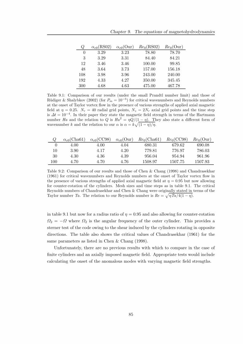
Chapter 9. The equations of magnetohydrodynamics
Q αc0(RS02) αc0(Our) Re0(RS02) Re0(Our)
0 3.29 3.23 78.80 78.703 3.29 3.31 84.40 84.21
12 3.46 3.46 100.00 99.8548 3.64 3.73 157.00 156.18
108 3.98 3.96 243.00 240.00192 4.33 4.27 350.00 345.45300 4.68 4.63 475.00 467.78
Table 9.1: Comparison of our results (under the small Prandtl number limit) and those ofRudiger & Shalybkov (2002) (for Pm = 10−5) for critical wavenumbers and Reynolds numbersat the onset of Taylor vortex flow in the presence of various strengths of applied axial magneticfield at η = 0.25. Nr = 40 radial grid points, Nz = 2Nr axial grid points and the time stepis ∆t = 10−4. In their paper they state the magnetic field strength in terms of the Hartmannnumber Ha and the relation to Q is Ha2 = ηQ/(1 − η). They also state a different form ofwavenumber k and the relation to our α is α = k
√
(1 − η)/η.
Q αc0(Cha61) αc0(CC98) αc0(Our) Re0(Cha61) Re0(CC98) Re0(Our)
0 4.00 4.00 4.04 680.31 679.62 690.0810 3.90 4.17 4.20 779.81 776.97 786.0330 4.30 4.36 4.39 956.04 954.94 961.96
100 4.70 4.70 4.76 1508.97 1507.75 1507.93
Table 9.2: Comparison of our results and those of Chen & Chang (1998) and Chandrasekhar(1961) for critical wavenumbers and Reynolds numbers at the onset of Taylor vortex flow inthe presence of various strengths of applied axial magnetic field at η = 0.95 but now allowingfor counter-rotation of the cylinders. Mesh sizes and time steps as in table 9.1. The criticalReynolds numbers of Chandrasekhar and Chen & Chang were originally stated in terms of theTaylor number Ta. The relation to our Reynolds number is Re =
√
ηTa/4(1 − η).
in table 9.1 but now for a radius ratio of η = 0.95 and also allowing for counter-rotation
Ω2 = −Ω where Ω2 is the angular frequency of the outer cylinder. This provides a
sterner test of the code owing to the shear induced by the cylinders rotating in opposite
directions. The table also shows the critical values of Chandrasekhar (1961) for the
same parameters as listed in Chen & Chang (1998).
Unfortunately, there are no previous results with which to compare in the case of
finite cylinders and an axially imposed magnetic field. Appropriate tests would include
calculating the onset of the anomalous modes with varying magnetic field strengths.
85
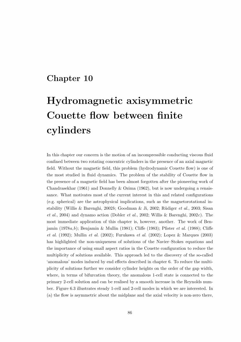
Chapter 10
Hydromagnetic axisymmetric
Couette flow between finite
cylinders
In this chapter our concern is the motion of an incompressible conducting viscous fluid
confined between two rotating concentric cylinders in the presence of an axial magnetic
field. Without the magnetic field, this problem (hydrodynamic Couette flow) is one of
the most studied in fluid dynamics. The problem of the stability of Couette flow in
the presence of a magnetic field has been almost forgotten after the pioneering work of
Chandrasekhar (1961) and Donnelly & Ozima (1962), but is now undergoing a renais-
sance. What motivates most of the current interest in this and related configurations
(e.g. spherical) are the astrophysical implications, such as the magnetorotational in-
stability (Willis & Barenghi, 2002b; Goodman & Ji, 2002; Rudiger et al., 2003; Sisan
et al., 2004) and dynamo action (Dobler et al., 2002; Willis & Barenghi, 2002c). The
most immediate application of this chapter is, however, another. The work of Ben-
jamin (1978a,b); Benjamin & Mullin (1981); Cliffe (1983); Pfister et al. (1988); Cliffe
et al. (1992); Mullin et al. (2002); Furukawa et al. (2002); Lopez & Marques (2003)
has highlighted the non-uniqueness of solutions of the Navier–Stokes equations and
the importance of using small aspect ratios in the Couette configuration to reduce the
multiplicity of solutions available. This approach led to the discovery of the so-called
‘anomalous’ modes induced by end effects described in chapter 6. To reduce the multi-
plicity of solutions further we consider cylinder heights on the order of the gap width,
where, in terms of bifurcation theory, the anomalous 1-cell state is connected to the
primary 2-cell solution and can be realised by a smooth increase in the Reynolds num-
ber. Figure 6.3 illustrates steady 1-cell and 2-cell modes in which we are interested. In
(a) the flow is asymmetric about the midplane and the axial velocity is non-zero there,
86
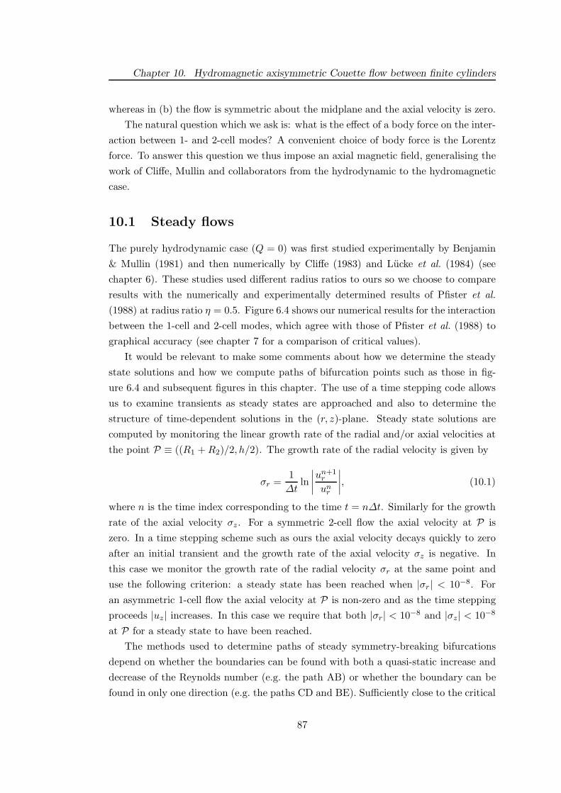
Chapter 10. Hydromagnetic axisymmetric Couette flow between finite cylinders
whereas in (b) the flow is symmetric about the midplane and the axial velocity is zero.
The natural question which we ask is: what is the effect of a body force on the inter-
action between 1- and 2-cell modes? A convenient choice of body force is the Lorentz
force. To answer this question we thus impose an axial magnetic field, generalising the
work of Cliffe, Mullin and collaborators from the hydrodynamic to the hydromagnetic
case.
10.1 Steady flows
The purely hydrodynamic case (Q = 0) was first studied experimentally by Benjamin
& Mullin (1981) and then numerically by Cliffe (1983) and Lucke et al. (1984) (see
chapter 6). These studies used different radius ratios to ours so we choose to compare
results with the numerically and experimentally determined results of Pfister et al.
(1988) at radius ratio η = 0.5. Figure 6.4 shows our numerical results for the interaction
between the 1-cell and 2-cell modes, which agree with those of Pfister et al. (1988) to
graphical accuracy (see chapter 7 for a comparison of critical values).
It would be relevant to make some comments about how we determine the steady
state solutions and how we compute paths of bifurcation points such as those in fig-
ure 6.4 and subsequent figures in this chapter. The use of a time stepping code allows
us to examine transients as steady states are approached and also to determine the
structure of time-dependent solutions in the (r, z)-plane. Steady state solutions are
computed by monitoring the linear growth rate of the radial and/or axial velocities at
the point P ≡ ((R1 +R2)/2, h/2). The growth rate of the radial velocity is given by
σr =1
∆tln
∣
∣
∣
∣
un+1r
unr
∣
∣
∣
∣
, (10.1)
where n is the time index corresponding to the time t = n∆t. Similarly for the growth
rate of the axial velocity σz. For a symmetric 2-cell flow the axial velocity at P is
zero. In a time stepping scheme such as ours the axial velocity decays quickly to zero
after an initial transient and the growth rate of the axial velocity σz is negative. In
this case we monitor the growth rate of the radial velocity σr at the same point and
use the following criterion: a steady state has been reached when |σr| < 10−8. For
an asymmetric 1-cell flow the axial velocity at P is non-zero and as the time stepping
proceeds |uz| increases. In this case we require that both |σr| < 10−8 and |σz| < 10−8
at P for a steady state to have been reached.
The methods used to determine paths of steady symmetry-breaking bifurcations
depend on whether the boundaries can be found with both a quasi-static increase and
decrease of the Reynolds number (e.g. the path AB) or whether the boundary can be
found in only one direction (e.g. the paths CD and BE). Sufficiently close to the critical
87
Chapter 10. Hydromagnetic axisymmetric Couette flow between finite cylinders
Reynolds number for the onset of asymmetry σz at P is approximately constant. If
σz > 0 then |uz| is increasing and an asymmetric state sets in; if σz < 0 then |uz|
is decreasing and a symmetric state sets in. The boundary AB was found in the
following way: the Reynolds number is set to a value just below critical and once σz
is constant (i.e. σz varies by less than 10−8 between successive time steps) the sign
of σz is checked. The Reynolds number is then automatically stepped in arbitrarily
small increments until a change of sign in σz is detected. Once this change of sign
occurs a bisection method is employed to determine the critical Reynolds number. At
the critical Reynolds number |σz| is found to be less than 10−6. Finding the boundary
CD is a little more difficult since it can be found only by a quasi-static decrease of the
Reynolds number after a sudden start of the cylinder to a Reynolds number above the
critical value. The Reynolds number is automatically decreased in small steps until σz
switches sign from negative to positive (indicating a transition from a symmetric to an
asymmetric state). It is then no longer possible to increase the Reynolds number again,
since CD can only be found by a decrease in the Reynolds number. To overcome this
difficulty the Reynolds number is instantaneously set to zero and then to a value above
critical after the axial velocity has decayed sufficiently. In this way it is possible to carry
out the bisection method using the two Reynolds numbers between which a change of
sign of σz occurs, approaching the critical value only from above the boundary CD. At
the critical Reynolds number |σz| is again found to be less than 10−6. The path BE
and the hysteresis region are found in similar ways with further minor modifications.
Figure 10.1 shows the same bifurcation diagram as in figure 6.4 but now including
various strengths of applied magnetic field (Q 6= 0). The general trend is that, by
increasing the magnetic field, the instability to 1-cell flows is pushed to higher Reynolds
numbers, so 2-cell flows are more likely. In a qualitative sense, this is consistent with
the findings of Chandrasekhar (1961) that, for Γ → ∞ and Q > 100, the characteristic
axial wavelength decreases. Schulz et al. (2003) considered the effect of outer cylinder
rotation on the transition between the 1- and 2-cell states and found that symmetric
2-cell flows were stabilised by co-rotation of the cylinders with the stabilising effect
being greater the larger the rotation rate of the outer cylinder; in fact for a certain
value of the outer cylinder Reynolds number (at Γ = 1) the 2-cell state remained stable
for all rotation rates of the inner cylinder examined. We have found a similar effect
with the application of a magnetic field; for the same aspect ratio (Γ = 1) there is a
critical Q at which the 1-cell state is no longer realisable. This can be seen in figure 10.1
where, with Q = 100, the 1-cell state no longer exists for a quasi-static increase of the
Reynolds number.
This destabilisation of the 2-cell flow is less pronounced as the aspect ratio is de-
creased and all curves seem to tend to an asymptote at approximately Γ = 0.2. It was
88

Chapter 10. Hydromagnetic axisymmetric Couette flow between finite cylinders
100
300
500
700
900
0.2 0.4 0.6 0.8 1.0 1.2 1.4 1.6 1.8
Rec
Γ
Figure 10.1: Critical Reynolds number Rec versus aspect ratio Γ for the transition between the1- and 2-cell flows (as figure 6.4) in the presence of various applied magnetic fields Q. Q = 0( ), Q = 5 ( ), Q = 10 ( ), Q = 50 ( ), Q = 100 ( ).
shown by Mullin et al. (2002) at various radius ratios that there is a critical value of Γ
below which the 1-cell flow no longer exists, and the flow is symmetric and unique, at
least for not too large Reynolds numbers. The left-hand side of figure 10.1 shows that
the application of a magnetic field does not alter Mullin et al.’s critical aspect ratio.
There is another critical aspect ratio Γc (corresponding to the point C in figure 6.4)
at which the 1-cell flow is no longer realisable by a quasi-static increase of the Reynolds
number across AB or decrease across CD. Figure 10.2 shows Γc versus Q; Γc increases
with increasing Q for Q > 10 but then for Q ? 10 it decreases with increasing Q.
Figures 10.3 and 10.4 show contour plots of various fields in the presence of an
applied magnetic field, Q = 100. The aspect ratio of Γ = 0.97 is chosen to allow both
the 1- and 2-cell flows to exist at the same Reynolds number, Re = 500, ensuring a
fairer comparison, with only the route taken through parameter space differing in each
case. It is apparent from both sets of figures that the cells are compressed toward the
inner cylinder. This is in contrast to the case of no magnetic field, Q = 0, as in figure 6.3
(albeit at slightly different aspect ratio and Reynolds number) where the cells are much
more centrally located. Goodman & Ji (2002) show similar contour plots of the stream
function and azimuthal magnetic field (as well as the flux function and azimuthal
velocity perturbation) with both perfectly conducting and insulating boundaries for
the infinite cylinder case. From their plots (with conducting boundaries) it is also
89
Chapter 10. Hydromagnetic axisymmetric Couette flow between finite cylinders
0.95
1.05
1.15
1.25
1.35
1.45
0 20 40 60 80 100
Γc
Q
Figure 10.2: Critical aspect ratio Γc versus Q (the point at which the 1-cell flow is no longerrealisable by a quasi-static increase of Re across the curve AB or decrease across the curve CD).
evident that the cells are compressed toward the inner cylinder under the influence of
a magnetic field.
10.2 Time-dependent flows
The previous section detailed only steady flows. Time-dependent 1- and 2-cell states at
aspect ratios up to Γ ≈ 0.5 have been described in the literature. Pfister et al. (1988)
discovered axisymmetric oscillations for Γ ? 0.35; this time-dependence disappeared
for Γ ? 0.55. Furukawa et al. (2002) confirmed the existence of time-dependence in
this region. Lopez & Marques (2003) extended the study to include non-axisymmetric
motion for a fixed aspect ratio of Γ = 0.5 and found interesting dynamics including
double Hopf bifurcations, Neimark–Sacker bifurcations to a modulated rotating wave,
and saddle-node-infinite-period bifurcations. These time-dependent solutions for Γ >
0.5 are not included in figure 6.4 for clarity. In this chapter we concentrate on what
happens to the right-hand side of figure 6.4, where we have discovered that the magnetic
field induces time-dependence at relatively small Reynolds numbers.
Figure 10.5 shows the critical Reynolds number Retd for the onset of time-dependent
flow versus aspect ratio at various strengths of magnetic field. For Q = 0, the 1-cell
mode realised by a quasi-static increase in the Reynolds number across AB undergoes
a Hopf bifurcation to the unsteady state across the curve XY. The transition between
90
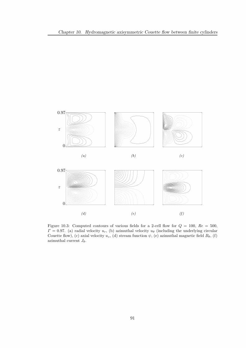
Chapter 10. Hydromagnetic axisymmetric Couette flow between finite cylinders
0.97
z
0
(a)
(b)
(c)
0.97
z
0
(d)
(e)
(f)
Figure 10.3: Computed contours of various fields for a 2-cell flow for Q = 100, Re = 500,Γ = 0.97. (a) radial velocity ur, (b) azimuthal velocity uθ (including the underlying circularCouette flow), (c) axial velocity uz, (d) stream function ψ, (e) azimuthal magnetic field Bθ, (f)azimuthal current Jθ.
91
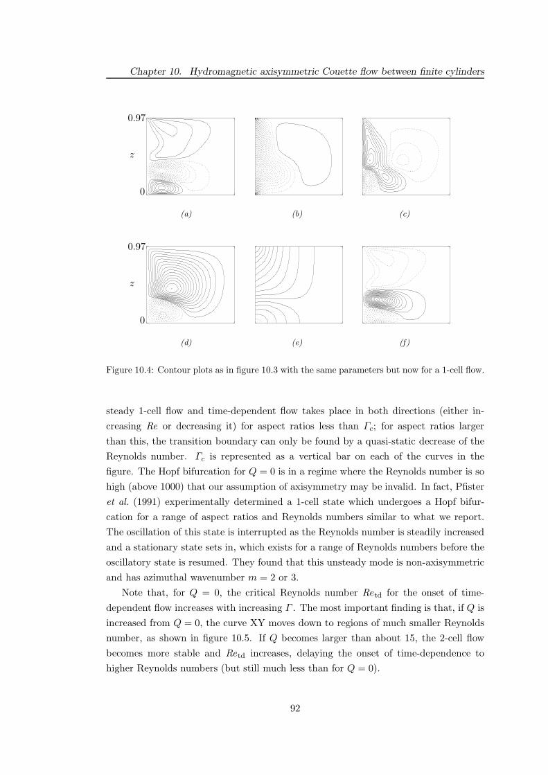
Chapter 10. Hydromagnetic axisymmetric Couette flow between finite cylinders
0.97
z
0
(a)
(b)
(c)
0.97
z
0
(d)
(e)
(f)
Figure 10.4: Contour plots as in figure 10.3 with the same parameters but now for a 1-cell flow.
steady 1-cell flow and time-dependent flow takes place in both directions (either in-
creasing Re or decreasing it) for aspect ratios less than Γc; for aspect ratios larger
than this, the transition boundary can only be found by a quasi-static decrease of the
Reynolds number. Γc is represented as a vertical bar on each of the curves in the
figure. The Hopf bifurcation for Q = 0 is in a regime where the Reynolds number is so
high (above 1000) that our assumption of axisymmetry may be invalid. In fact, Pfister
et al. (1991) experimentally determined a 1-cell state which undergoes a Hopf bifur-
cation for a range of aspect ratios and Reynolds numbers similar to what we report.
The oscillation of this state is interrupted as the Reynolds number is steadily increased
and a stationary state sets in, which exists for a range of Reynolds numbers before the
oscillatory state is resumed. They found that this unsteady mode is non-axisymmetric
and has azimuthal wavenumber m = 2 or 3.
Note that, for Q = 0, the critical Reynolds number Retd for the onset of time-
dependent flow increases with increasing Γ . The most important finding is that, if Q is
increased from Q = 0, the curve XY moves down to regions of much smaller Reynolds
number, as shown in figure 10.5. If Q becomes larger than about 15, the 2-cell flow
becomes more stable and Retd increases, delaying the onset of time-dependence to
higher Reynolds numbers (but still much less than for Q = 0).
92
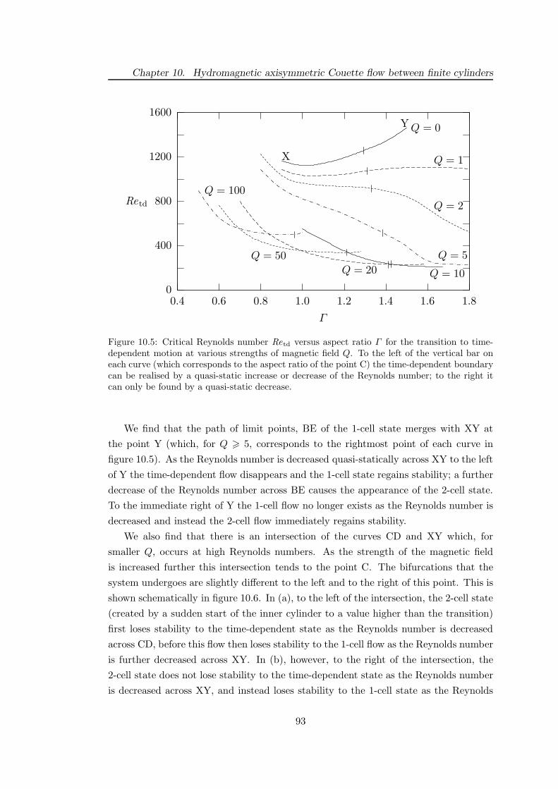
Chapter 10. Hydromagnetic axisymmetric Couette flow between finite cylinders
0
400
800
1200
1600
0.4 0.6 0.8 1.0 1.2 1.4 1.6 1.8
Retd
Γ
X
YQ = 0
Q = 1
Q = 2
Q = 5
Q = 10Q = 20
Q = 50
Q = 100
Figure 10.5: Critical Reynolds number Retd versus aspect ratio Γ for the transition to time-dependent motion at various strengths of magnetic field Q. To the left of the vertical bar oneach curve (which corresponds to the aspect ratio of the point C) the time-dependent boundarycan be realised by a quasi-static increase or decrease of the Reynolds number; to the right itcan only be found by a quasi-static decrease.
We find that the path of limit points, BE of the 1-cell state merges with XY at
the point Y (which, for Q > 5, corresponds to the rightmost point of each curve in
figure 10.5). As the Reynolds number is decreased quasi-statically across XY to the left
of Y the time-dependent flow disappears and the 1-cell state regains stability; a further
decrease of the Reynolds number across BE causes the appearance of the 2-cell state.
To the immediate right of Y the 1-cell flow no longer exists as the Reynolds number is
decreased and instead the 2-cell flow immediately regains stability.
We also find that there is an intersection of the curves CD and XY which, for
smaller Q, occurs at high Reynolds numbers. As the strength of the magnetic field
is increased further this intersection tends to the point C. The bifurcations that the
system undergoes are slightly different to the left and to the right of this point. This is
shown schematically in figure 10.6. In (a), to the left of the intersection, the 2-cell state
(created by a sudden start of the inner cylinder to a value higher than the transition)
first loses stability to the time-dependent state as the Reynolds number is decreased
across CD, before this flow then loses stability to the 1-cell flow as the Reynolds number
is further decreased across XY. In (b), however, to the right of the intersection, the
2-cell state does not lose stability to the time-dependent state as the Reynolds number
is decreased across XY, and instead loses stability to the 1-cell state as the Reynolds
93

Chapter 10. Hydromagnetic axisymmetric Couette flow between finite cylinders
replacemen
0
uz
ReRec1 Rec2Re td
C1
C2C2
Ctd
(a)
0
uz
ReRec1 Rec2 Re td
C1
C2C2
Ctd
(b)
Figure 10.6: Schematic bifurcation diagrams (a) to the left and (b) to the right of the inter-section point of curves CD and XY. The arrows denote the critical Reynolds number at whichthe 2-cell flow loses stability to (a) the time-dependent flow and (b) the 1-cell flow.
number is decreased across CD.
Figure 10.7 shows the frequency f of the oscillations at the onset of time-dependence
versus the aspect ratio Γ at various strengths of applied magnetic field Q. Here, f is
non-dimensionalised with respect to the inner cylinder angular frequency Ω.
Note that the curves of f versus Γ follow the same trend as the curves of Retd versus
Γ of figure 10.5: f is lower the higher Q is. All frequencies f which we have found
are much higher (at least one order of magnitude higher) than values of f reported by
Pfister et al. (1988) in the absence of a magnetic field.
The nature of these time-dependent flows is revealed by figure 10.8, which shows
contour plots of the stream function at various times over one period for Q = 10.
Initially, in (a), the flow has the familiar 1-cell structure with a large main vortex
and a smaller vortex in the corner near to the inner cylinder. Then the large vortex is
deformed slightly and a very weak third vortex begins to appear near the inner cylinder
at the upper-left corner (not visible in the contour plot). As the third vortex travels
down the inner cylinder it becomes stronger as shown in (b). In (c) the third vortex
begins to merge with the second vortex in the lower-left corner until a vortex roughly
twice the size of the original second small vortex is produced in (d). In (e) this new
vortex spreads across the gap towards the outer cylinder and splits in two in (f), before
the process is repeated again. Although there is no direct evidence that this flow is
the same as the one observed by Lensch (1988) and Pfister et al. (1991) the spatial–
temporal dependence does bear a qualitative resemblance to their non-axisymmetric
time-dependent flow; the main difference being that the third vortex which appears
near the inner cylinder can travel all the way around the first vortex.
We have also discovered the existence of a time-dependent 2-cell flow which exists
for both Q = 0 and Q 6= 0. Contour snapshots of this flow can be seen in figure 10.9
94

Chapter 10. Hydromagnetic axisymmetric Couette flow between finite cylinders
0.2
0.4
0.6
0.8
0.4 0.6 0.8 1.0 1.2 1.4 1.6 1.8
f
Γ
Q = 0Q = 1
Q = 2
Q = 5
Q = 10Q = 20Q = 50
Q = 100
Figure 10.7: Frequency f of the oscillations at the onset of axisymmetric time-dependenceversus aspect ratio Γ at various strengths of magnetic field Q. f is non-dimensionalised withrespect to the inner cylinder angular frequency Ω. The relation between f and ω, the frequencywhich has been non-dimensionalised with respect to the diffusion time δ2/ν is ω = Re(1−η)f/η.
for Q = 10, Re = 700, and Γ = 1.3. The effect is quite subtle and not as easy to see as
the 1-cell time-dependence; the oscillation is caused by each cell, in turn, tilting and
growing larger across the midplane. Figures 10.10 and 10.11 show enlarged views of
the right-hand side of the transition diagrams for Q = 0 and Q = 10. They show the
interaction of the 1-cell and 2-cell steady flows, the 1-cell time-dependent flow (XY) and
also the 2-cell time-dependent flow (ST). We found this flow by instantaneously setting
the Reynolds number, from seed, to a value above the transition, and then decreasing
the Reynolds number until a new flow structure emerged. For the case Q = 0, and
for the aspect ratios considered, the time-dependent 2-cell flow has a critical Reynolds
number below that of the time-dependent 1-cell flow. For Q = 10 the situation is
reversed. For both Q = 0 and Q = 10, as the Reynolds number is decreased across
ST, the time-dependent 2-cell flow loses stability to the steady 2-cell flow. There is one
exception to this for Q = 0 at the point S. Here, the curve takes a sharp upturn and
the time-dependent 2-cell flow immediately loses stability to the steady 1-cell flow as
ST is crossed (ST and CD do not actually meet). Further to the left of this point it
is increasingly difficult to find the boundary of either CD or ST as the curves become
nearly vertical. Because of this, any critical Reynolds numbers found are likely to be
inaccurate. A similar situation arises for Q = 10 although it does not appear that
95

Chapter 10. Hydromagnetic axisymmetric Couette flow between finite cylinders
1.7
z
0
(a)
(b)
(c)
1.7
z
0
(d)
(e)
(f)
Figure 10.8: Snapshots of the stream function over one period for the time-dependent flowfor Q = 10, Re = 400, and Γ = 1.7. (a) t = 25.9857, (b) t = 25.9962, (c) t = 25.9998, (d)t = 26.0034, (e) t = 26.0091, (f) t = 26.0142.
96

Chapter 10. Hydromagnetic axisymmetric Couette flow between finite cylinders
1.3
z
0
(a)
(b)
(c)
1.3
z
0
(d)
(e)
(f)
Figure 10.9: Snapshots of the stream function over one period for the time-dependent 2-cellflow for Q = 10, Re = 700, and Γ = 1.3. (a) t = 4.0453, (b) t = 4.0477, (c) t = 4.0500, (d)t = 4.0524, (e) t = 4.0548, (f) t = 4.0572.
the curve ST becomes too steep. To the left of the points D and S in both figures,
a decrease of 0.01 in the aspect ratio does not allow the boundaries CD or ST to be
extended further. Further calculations have shown the existence of the time-dependent
2-cell flow at Q = 5, but more work is necessary to explore the existence of this flow
at other strengths of applied magnetic field and to better understand the transition
boundaries for Q = 0 and Q = 10.
10.3 Summary
To summarise the results in this chapter, the presence of a body force, such as an
axially imposed magnetic field, does not reduce the multiplicity of solutions available
even at small aspect ratio, which was revealed by Benjamin, Mullin, Pfister and others.
If one increases the magnetic field, however, the general trend is that a larger Reynolds
97

Chapter 10. Hydromagnetic axisymmetric Couette flow between finite cylinders
0
400
800
1200
1600
0.8 1.0 1.2 1.4 1.6
Re
Γ
B C
D
E
ST
X
Y
Figure 10.10: Reynolds number versus aspect ratio highlighting the boundary (ST) for thetransition to the 2-cell time-dependent flow, for Q = 0.
100
300
500
700
0.8 1.0 1.2 1.4 1.6 1.8
Re
Γ
BC
D
E
ST
X
Y
Figure 10.11: Reynolds number versus aspect ratio as in figure 10.10 but now for Q = 10.
98

Chapter 10. Hydromagnetic axisymmetric Couette flow between finite cylinders
number is necessary to obtain steady 1-cell states, that is, steady 2-cell states are more
stable. We have also found that, under an applied magnetic field, it is easy to excite
time-dependent flows at relatively small Reynolds numbers.
99
Chapter 11
Conclusions and further work
At the beginning of this thesis (chapters 2 and 3) we set up the governing equations
and a suitable numerical formulation for the study of modulated Taylor–Couette flow
between cylinders of infinite height.
In chapter 4 we looked at a simple variation of the modulated problem where the
inner cylinder’s rotation was modulated harmonically about zero mean (as opposed to
the more widely studied problem of modulation about a non-zero mean) and the outer
cylinder was held at rest. The consequence of the modulation was to give rise to two
classes of solution — reversing Taylor vortex flow (RTVF) and non-reversing Taylor
vortex flow (NRTVF). In RTVF the Taylor vortices that form always reverse their
rotation direction when the inner cylinder changes its direction; in NRTVF the Taylor
vortices always rotate in the same direction despite the change in rotation direction of
the inner cylinder. The initial (axisymmetric) investigation into these two flows was
carried out over a wide range of modulation frequencies, amplitudes and radius ratios
and the reversing/non-reversing effect was found to be robust in the sense that it exists
over the range of parameter values explored.
Chapter 5 was an extension of the reversing and non-reversing results of chapter 4
to allow for the possibility of non-axisymmetric motion. In the steady problem it is
well known that Taylor vortices become unstable to non-axisymmetric perturbations
at some critical Reynolds number which depends on the radius ratio; this instability
gives rise to azimuthal waves (the wavy modes) which rotate around the inner cylinder
at some wavespeed. The goal of chapter 5 was to determine whether the presence of
the azimuthal instability destroyed either of the reversing/non-reversing solutions. The
answer to this question is negative — both reversing and non-reversing solutions exist
in the wavy modes regime, the most interesting discovery being that the non-reversing
solution is a spiral mode.
The results obtained under the infinite cylinder approximation are very helpful in
gaining an insight to the flow structures which may be possible but it has been shown
100
Chapter 11. Conclusions and further work
that the effects of the end-plates which are necessarily attached in an experimental
apparatus cannot be ignored and, in fact, some solutions which exist in the realistic
geometry do not exist under the infinite cylinder approximation.
Chapter 6 gave an introduction to the so-called ‘anomalous’ modes which only exist
in finite geometry. They are disconnected from the primary flow and exist at much
higher Reynolds numbers than the onset of Taylor vortex flow in the infinite cylinder
case. They are distinguished by the apparent counter-intuitive rotation direction of the
end cells and also by the existence of flows which are asymmetric about the midplane.
We also used the homotopy parameter τ which was introduced by Schaeffer (1980)
to theoretically continuously deform the end boundary conditions from the infinite
cylinder case to the finite cylinder case. We also remarked on the non-uniqueness of
the solutions which exist in finite geometry and how very short cylinders are used to
attempt to combat this non-uniqueness.
Chapter 7 detailed a second numerical formulation which allows the existence of
fixed end-plates using the well-known stream function–vorticity formulation which we
used in the subsequent chapters.
Chapter 8 was another extension to the (axisymmetric) results of chapter 4. Here,
we attempted to determine what effect (if any) the presence of the end-plates had
on the reversing and non-reversing solutions. We found that, again, both solutions
still exist but that there is a now a strong dependence on the height of the cylinders.
For cylinders which are of ‘intermediate’ height (see the chapter for the definition of
intermediate) there are no reversing solutions for any of the frequencies we explored
and only non-reversing solutions exist. There is then a further dependence on the
modulation amplitude which gives rise to non-reversing solutions with different numbers
of cells. Only when the cylinders are sufficiently long do reversing solutions become
possible, and then the most interesting aspect of these solutions is that not all the
cells in the gap reverse their rotation direction. Furthermore, the number of cells in
the reversing solution now depends on the Reynolds number within the cycle rather
than on the modulation amplitude. For higher frequencies we recovered the results
from the infinite cylinder approximation whereby no reversing flows are possible. The
dynamics were found to be quite complicated for the range of cylinder heights where
there is competition between the reversing and non-reversing solutions. We concluded
the chapter with a look at cylinders with heights of the order of the gap width and
found flow structures which consisted of oscillations between one and two cells and
also novel (time-dependent) ‘side-by-side’ flows where the cells are positioned radially
instead of axially.
The final part of this thesis moved away from temporal forcing and looked at the
effect of a body force in the form of an externally applied axial magnetic field. Chapter 9
101

Chapter 11. Conclusions and further work
extended the numerical code of chapter 7 to include the magnetic field and this was used
in chapter 10. In trying to reduce the multiplicity of solutions we restricted ourselves
to looking at very short cylinders where only 1- and 2-cell flows exist. There were
two main results of this chapter. The first was to find that the stability of the 2-cell
flow is greatly enhanced under the influence of the magnetic field except in incredibly
compressed cylinders where the enhancement of stability is much less. The second
was that axisymmetric time-dependent solutions are much easier to excite under the
influence of a magnetic field, in some cases reducing the Reynolds number for the onset
from about 1500 to about 300.
There is plenty of scope for further work on the results in this thesis. The existence
of Taylor vortices whose meridional circulation is not affected by the direction of the
basic azimuthal flow is visible in some of the recent nonlinear numerical simulations of
Zhang (2002) of time modulated spherical Couette flow. In light of this and also the
results of the flows between finite height cylinders NRTVF is probably a robust effect
which should be investigated experimentally.
In cylindrical geometry it should be possible to control the Ekman circulation by
using a non-uniform gap which produces a spatial ramp of the Reynolds number (as
done by Ning et al., 1990; Wiener et al., 1999, for example) so that the flow is subcritical
near the top and bottom ends. This may enable some connection to be made between
the reversing and non-reversing solutions in finite and infinite geometries.
In finite geometry it is also possible to vary the motion of the end-plates to provide
different boundary conditions. They can either be attached to the outer cylinder (and
so at rest as in this thesis) or they can rotate with the inner cylinder. (A combination
of these is also possible.) It would be interesting to examine the effect of these different
boundary conditions on the reversing and non-reversing flows.
Hydromagnetic Couette flow seems to be a very rich system, and the work presented
here is only an initial investigation of axisymmetric flows in a restricted region of
parameter space. Further work should consider time-dependent 2-cell flows under a
larger magnetic field, what happens in cylinders which are very compressed where
the flow solutions appear to be unique, the effect of electrically insulating boundary
conditions and the possibility of non-axisymmetric motion. There is also the possibility
of applying the external magnetic field in the azimuthal direction as another variation.
As well as the above extensions to the work presented in this thesis there are other
opportunities for forcing the flow, for example, spatial forcing where the cylinders’ walls
are not straight but vary in a sinusoidal shape in the axial direction (see Koschmieder,
1975; Li & Khayat, 2004, for example). This spatial forcing could be combined with
temporal forcing as described in this thesis and/or with the body force of an applied
magnetic field. The ultimate goal would be to allow non-axisymmetric motion for any
102

Chapter 11. Conclusions and further work
of the problems in this thesis and also the problems outlined above.
103
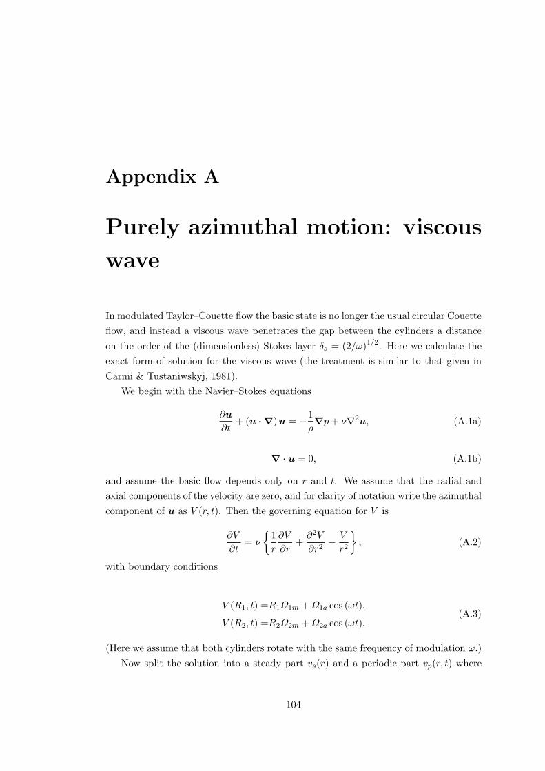
Appendix A
Purely azimuthal motion: viscous
wave
In modulated Taylor–Couette flow the basic state is no longer the usual circular Couette
flow, and instead a viscous wave penetrates the gap between the cylinders a distance
on the order of the (dimensionless) Stokes layer δs = (2/ω)1/2. Here we calculate the
exact form of solution for the viscous wave (the treatment is similar to that given in
Carmi & Tustaniwskyj, 1981).
We begin with the Navier–Stokes equations
∂u
∂t+ (u · ∇)u = −
1
ρ∇p+ ν∇2
u, (A.1a)
∇ · u = 0, (A.1b)
and assume the basic flow depends only on r and t. We assume that the radial and
axial components of the velocity are zero, and for clarity of notation write the azimuthal
component of u as V (r, t). Then the governing equation for V is
∂V
∂t= ν
1
r
∂V
∂r+∂2V
∂r2−V
r2
, (A.2)
with boundary conditions
V (R1, t) =R1Ω1m +Ω1a cos (ωt),
V (R2, t) =R2Ω2m +Ω2a cos (ωt).(A.3)
(Here we assume that both cylinders rotate with the same frequency of modulation ω.)
Now split the solution into a steady part vs(r) and a periodic part vp(r, t) where
104

Appendix A. Purely azimuthal motion: viscous wave
vs(r) is the underlying Couette flow. So
V (r, t) = vs(r) + vp(r, t). (A.4)
The steady Couette flow vs(r) satisfies
1
r
∂vs
∂r+∂2vs
∂r2−vs
r2= 0, (A.5)
with boundary conditions
vs(R1) =R1Ω1m,
vs(R2) =R2Ω2m,(A.6)
and thus has solution
vs(r) = Ar +B
r, (A.7)
where
A =Ω2mR
22 −Ω1mR
21
R22 −R2
1
, B =(Ω1m −Ω2m)R2
1R22
R22 −R2
1
. (A.8)
The periodic part vp(r, t) then satisfies
∂vp
∂t= ν
1
r
∂vp
∂r+∂2vp
∂r2−vp
r2
, (A.9)
with boundary conditions
vp(R1, t) =Ω1aR1 cos (ωt),
vp(R2, t) =Ω2aR2 cos (ωt).(A.10)
We now look for periodic solutions of the form
vp(r, t) = v(r)eiωt, (A.11)
with boundary conditions
v(R1) =R1Ω1a,
v(R2) =R2Ω2a.(A.12)
We then substitute expression (A.11) into equation (A.9) so
105
Appendix A. Purely azimuthal motion: viscous wave
d2v
dr2+
1
r
dv
dr−
iω
ν+
1
r2
v = 0. (A.13)
Now we make the transformation y = βr where β =√
iω/ν then d/dr ≡ βd/dy and
r = y/β, so equation (A.13) becomes
β2 d2v
dy2+β
yβ
dv
dy−
β2 +β2
y2
v = 0, (A.14)
which leads to
d2v
dy2+
1
y
dv
dy−
1 +1
y2
v = 0, (A.15)
which is a modified Bessel equation of order one. The solutions are a linear combination
of modified Bessel functions I1 and K1
v(y) = CI1(y) +DK1(y). (A.16)
Then C and D are found so as to satisfy the boundary conditions
v(βR1) =R1Ω1a,
v(βR2) =R2Ω2a.(A.17)
We then solve the linear system of equations
[
K1(βR1) I1(βR1)
K1(βR2) I1(βR2)
][
C
D
]
=
[
R1Ω1a
R2Ω2a
]
, (A.18)
which has the solution
C =I1(βR1)Ω2aR2 − I1(βR2)Ω1aR1
∆,
D =K1(βR2)Ω1aR1 −K1(βR1)Ω2aR2
∆,
(A.19)
where ∆ ≡ K1(βR2)I1(βR1) −K1(βR1)I1(βR2).
The full solution of the viscous wave is then
V (r, t) = vs(r) + <
v(βr)eiωt
. (A.20)
106

Appendix B
Boundary conditions
Using cylindrical coordinates, the stream function ψ is defined by ur = −(1/r)∂zψ and
uz = (1/r)∂rψ.
From the no-slip boundary condition at the cylinder walls, ur = 0 at r = R1 and
R2, we find that ∂zψ = 0 at r = R1 and R2. Integrating and setting the arbitrary
constant equal to zero we conclude that ψ = 0 at r = R1 and R2. Similarly, from the
condition uz = 0 at z = 0 and h we conclude that ψ = 0 at z = 0 and h.
Boundary conditions for the azimuthal vorticity ωθ must be derived from those for
ψ. The equation for the azimuthal vorticity is
ωθ = −1
r
∂2ψ
∂z2−
1
r
∂2ψ
∂r2+
1
r2∂ψ
∂r. (B.1)
The first r- and second z-derivatives vanish at the cylinder walls due to the no-slip
boundary conditions for uz, and hence, ωθ = (−1/r)∂rrψ at r = R1 and R2. Similarly,
ωθ = (−1/r)∂zzψ at z = 0 and h.
The electric field E must be continuous at the cylinder walls, so n ∧ (Ec − Ef ) =
0, where the superscript c and f refer to the electric field in the cylinder and fluid
respectively, and n is the unit normal to a cylinder wall (n = ±r).
In general, r ∧E = (0,−Ez , Eθ), so to match the electric field across the boundary
we require Ecz = Ef
z and Ecθ = Ef
θ . Using Ohm’s law J = σE, where J is the
current and σ the electrical conductivity, we then have (1/σc)Jcz = (1/σf )Jf
z and
(1/σc)Jcθ = (1/σf )Jf
θ .
Assuming that the cylinders are perfectly conducting, we take σc → ∞ and, from
the second equation we conclude that Jfθ = 0 at r = R1 and R2.
The boundary condition for the azimuthal magnetic field is obtained from the equa-
tion J = ∇ ∧ B; using (1/σc)Jcz = (1/σf )Jf
z with σc → ∞ we have (1/r)Bfθ + ∂rB
fθ −
(1/r)∂θBfr = 0, where the superscript f has the same meaning as before; assuming
axisymmetry we conclude that (1/r)Bfθ + ∂rB
fθ = 0 at r = R1 and R2.
107
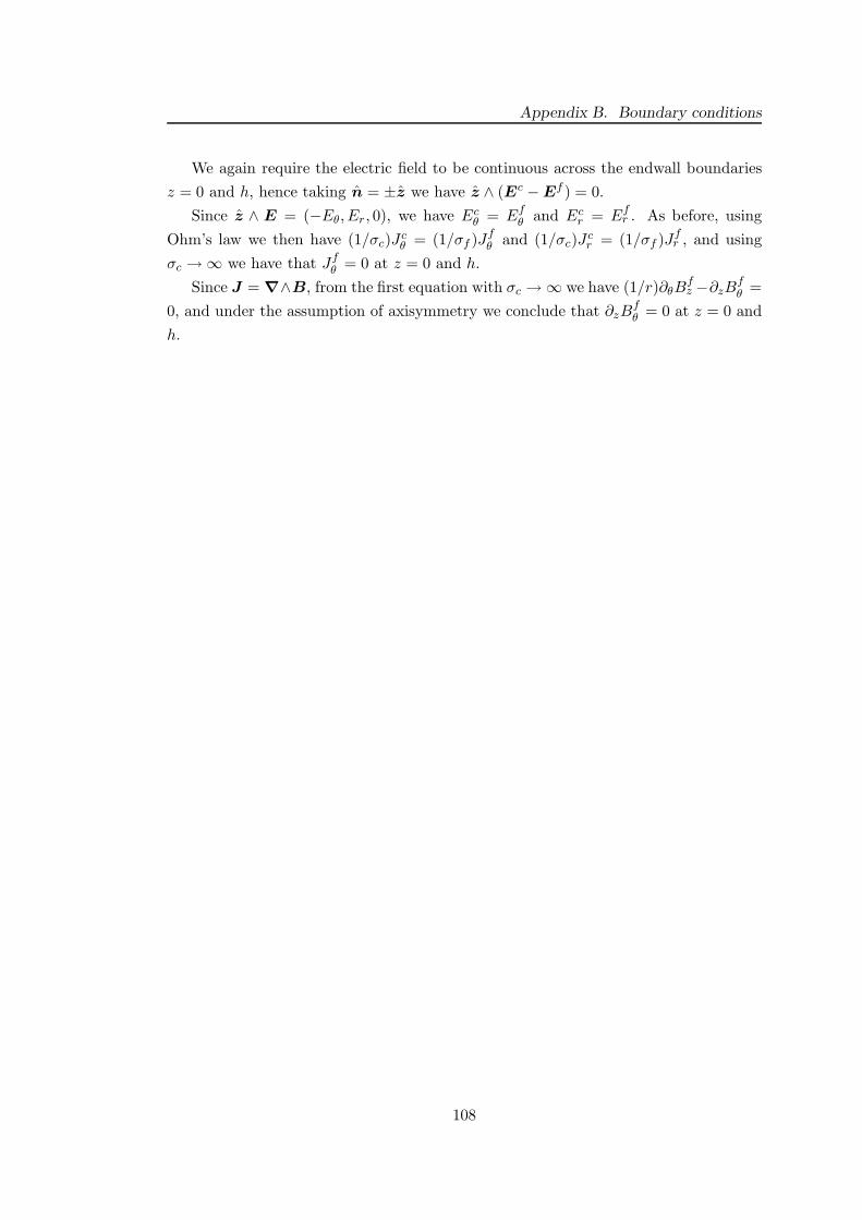
Appendix B. Boundary conditions
We again require the electric field to be continuous across the endwall boundaries
z = 0 and h, hence taking n = ±z we have z ∧ (Ec − Ef ) = 0.
Since z ∧ E = (−Eθ, Er, 0), we have Ecθ = Ef
θ and Ecr = Ef
r . As before, using
Ohm’s law we then have (1/σc)Jcθ = (1/σf )Jf
θ and (1/σc)Jcr = (1/σf )Jf
r , and using
σc → ∞ we have that Jfθ = 0 at z = 0 and h.
Since J = ∇∧B, from the first equation with σc → ∞ we have (1/r)∂θBfz −∂zB
fθ =
0, and under the assumption of axisymmetry we conclude that ∂zBfθ = 0 at z = 0 and
h.
108

Appendix C
Critical wavenumbers and
Reynolds numbers
Here, we give tables showing critical wavenumbers and Reynolds numbers for the onset
of steady and modulated Taylor vortex flow at various radius ratios and frequencies.
We also tabulate some critical values for the interaction between the 1- and 2-cell states
given in figure 6.4.
η αc0(Our) αc0(Rob65) Re0(Our) Re0(Rob65)
0.2 – 3.253 – 88.1280.28 – 3.222 – 75.0990.3 3.216 – 73.223 –0.36 – 3.195 – 69.5410.5 3.163 3.163 68.186 68.1860.6 3.149 – 71.715 –0.65 – 3.143 – 74.9620.7 3.140 – 79.490 –0.75 3.136 3.136 85.775 85.7760.8 3.133 – 94.733 –0.85 – 3.130 – 108.3120.875 – 3.130 – 118.1570.9 3.129 3.129 131.614 131.6130.925 – 3.128 – 151.4760.95 3.128 3.128 184.984 184.9810.9625 – 3.127 – 213.2270.975 – 3.127 – 260.948
Table C.1: Steady critical wavenumbers αc0 and Reynolds numbers Re0 of our code and thoseof Roberts (1965) for the onset of Taylor vortex flow at various radius ratios η.
109
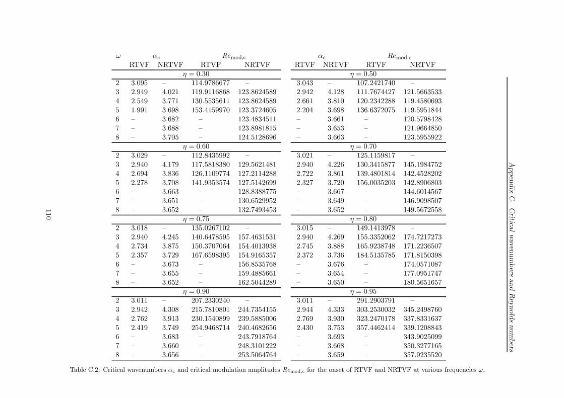
Appen
dix
C.
Critica
lw
aven
um
bers
and
Rey
nold
snum
bers
ω αc Remod,c αc Remod,c
RTVF NRTVF RTVF NRTVF RTVF NRTVF RTVF NRTVFη = 0.30 η = 0.50
2 3.095 – 114.9786677 – 3.043 – 107.2421740 –3 2.949 4.021 119.9116868 123.8624589 2.942 4.128 111.7674427 121.56635334 2.549 3.771 130.5535611 123.8624589 2.661 3.810 120.2342288 119.45806935 1.991 3.698 153.4159970 123.3724605 2.204 3.698 136.6372075 119.59518446 – 3.682 – 123.4834511 – 3.661 – 120.57984287 – 3.688 – 123.8981815 – 3.653 – 121.96648508 – 3.705 – 124.5128696 – 3.663 – 123.5955922
η = 0.60 η = 0.702 3.029 – 112.8435992 – 3.021 – 125.1159817 –3 2.940 4.179 117.5818380 129.5621481 2.940 4.226 130.3415877 145.19847524 2.694 3.836 126.1109774 127.2114288 2.722 3.861 139.4801814 142.45282025 2.278 3.708 141.9353574 127.5142699 2.327 3.720 156.0035203 142.89068036 – 3.663 – 128.8388775 – 3.667 – 144.60145677 – 3.651 – 130.6529952 – 3.649 – 146.90985078 – 3.652 – 132.7493453 – 3.652 – 149.5672558
η = 0.75 η = 0.802 3.018 – 135.0267102 – 3.015 – 149.1413978 –3 2.940 4.245 140.6478595 157.4631531 2.940 4.269 155.3352062 174.72172734 2.734 3.875 150.3707064 154.4013938 2.745 3.888 165.9238748 171.22365075 2.357 3.729 167.6598395 154.9165357 2.372 3.736 184.5135785 171.81503986 – 3.673 – 156.8535768 – 3.676 – 174.05710877 – 3.655 – 159.4885661 – 3.654 – 177.09517478 – 3.652 – 162.5044289 – 3.650 – 180.5651657
η = 0.90 η = 0.952 3.011 – 207.2330240 – 3.011 – 291.2903791 –3 2.942 4.308 215.7810801 244.7354155 2.944 4.333 303.2530032 345.24987604 2.762 3.913 230.1540899 239.5885006 2.769 3.930 323.2470178 337.83316375 2.419 3.749 254.9468714 240.4682656 2.430 3.753 357.4462414 339.12088436 – 3.683 – 243.7918764 – 3.693 – 343.90250997 – 3.660 – 248.3101222 – 3.668 – 350.32771658 – 3.656 – 253.5064764 – 3.659 – 357.9235520
Table C.2: Critical wavenumbers αc and critical modulation amplitudes Remod,c for the onset of RTVF and NRTVF at various frequencies ω.
110
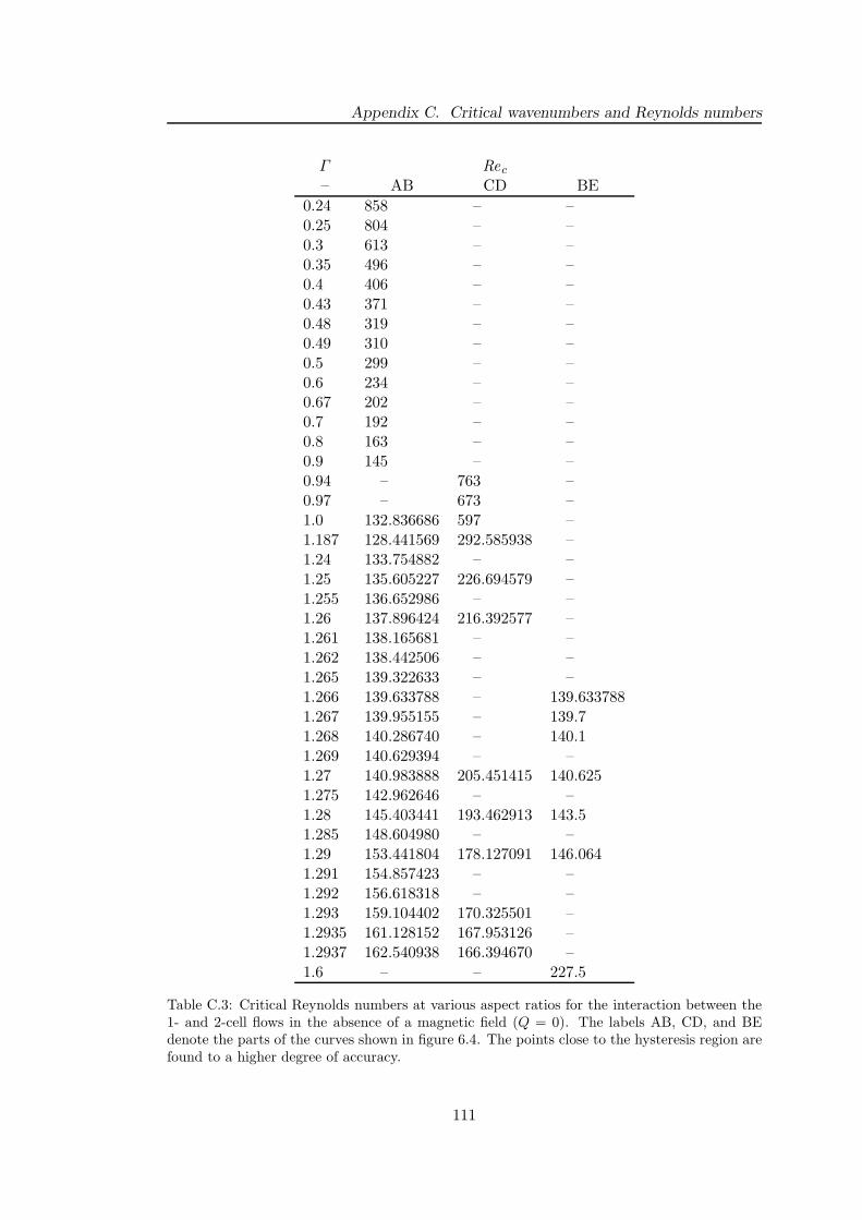
Appendix C. Critical wavenumbers and Reynolds numbers
Γ Rec
– AB CD BE
0.24 858 – –0.25 804 – –0.3 613 – –0.35 496 – –0.4 406 – –0.43 371 – –0.48 319 – –0.49 310 – –0.5 299 – –0.6 234 – –0.67 202 – –0.7 192 – –0.8 163 – –0.9 145 – –0.94 – 763 –0.97 – 673 –1.0 132.836686 597 –1.187 128.441569 292.585938 –1.24 133.754882 – –1.25 135.605227 226.694579 –1.255 136.652986 – –1.26 137.896424 216.392577 –1.261 138.165681 – –1.262 138.442506 – –1.265 139.322633 – –1.266 139.633788 – 139.6337881.267 139.955155 – 139.71.268 140.286740 – 140.11.269 140.629394 – –1.27 140.983888 205.451415 140.6251.275 142.962646 – –1.28 145.403441 193.462913 143.51.285 148.604980 – –1.29 153.441804 178.127091 146.0641.291 154.857423 – –1.292 156.618318 – –1.293 159.104402 170.325501 –1.2935 161.128152 167.953126 –1.2937 162.540938 166.394670 –1.6 – – 227.5
Table C.3: Critical Reynolds numbers at various aspect ratios for the interaction between the1- and 2-cell flows in the absence of a magnetic field (Q = 0). The labels AB, CD, and BEdenote the parts of the curves shown in figure 6.4. The points close to the hysteresis region arefound to a higher degree of accuracy.
111

Appendix D
Graphics and visualisation
The following is a brief outline of how to visualise the data which is output from the
numerical code. The descriptions that follow are tailored specifically for the output of
the codes used in this thesis, but it should be relatively straightforward to alter the
commands to cope with files in different formats.
D.1 Time-series plots
Time-series data is output in such a way so as to be readable by the free plotting
program gnuplot (http://www.gnuplot.info/). The commands which follow are based
on version 4.0 of gnuplot. The time-series data is output to the file u_growth.dat. It
contains 12 columns which are:
1. time
2. radial velocity at mid-height, mid-gap
3. radial velocity at z = 0, mid-gap
4. growth rate of the radial velocity
5. growth rate of the axial velocity
6. axial velocity at mid-height, mid-gap
7. stream function at mid-height, mid-gap
8. total azimuthal velocity at mid-height, mid-gap
9. azimuthal vorticity at quarter-height, mid-gap
10. azimuthal magnetic field at quarter-height, mid-gap
112
Appendix D. Graphics and visualisation
11. azimuthal current at mid-height, mid-gap
12. Reynolds number
Any one or more of these columns can be plotted using gnuplot with a command of
the form:
p "u_growth.dat" u m:n w l
which plots column n versus column m using lines as the style. Nearly all of the com-
mands in gnuplot can be shortened; the command above is the shortened form of
plot "u_growth.dat" using m:n with lines
Gnuplot will warn you if the shortened command is ambiguous.
Other common tasks include plotting two columns on the same graph which can be
done with:
p "u_growth.dat" u m:n w l, "" u p:q w l
which plots column n versus column m and column q versus column p on the same
graph with the same axis range. A more sophisticated command which does the same
plot but uses the left-hand y-axis for the column n data and the right-hand y-axis for
the column q data is as follows:
p "u_growth.dat" u m:n ax x1y1 w l, "" u p:q ax x1y2 w l
D.2 Contour plots
Data for contour plots is stored in numerous files containing a sequence of numbers.
The sequence of numbers represents the time at which a particular snapshot was taken.
The actual (dimensionless) diffusion time at which the snapshots are taken can be found
by multiplying by the time step.
All files except xsect*.dat contain data which can be plotted using gnuplot. The
prefix of the file determines what data is contained within, e.g. j for current, vr for
radial velocity, p for the stream function ψ, etc.
To plot the data use the command
113
Appendix D. Graphics and visualisation
sp "<filename>" u 1:2:3 w l
which by default shows a surface plot with no contours. Contours can be enabled with
set contour
and the number of contour levels can be set with
set cntrparam level n
where n is the number of levels. In gnuplot v4.0 the surface can be shaded with the
command
set pm3d
or the contours themselves can be shaded using
set pm3d map
which then disables the surface and shows a 2D (shaded) contour plot.
There are many other options to control the display of surface/contour plots. Gnu-
plot’s built-in help (accessed with the help command) has good descriptions of all the
possibilities. Start with help splot for a description of surface plots.
D.3 IDL contour plots
Additional files named xsect*.dat are also output which allows the possibility of
animations of contour plots using IDL (Interactive Data Language). These files are
read in to IDL using the jpeg.pro and jpeg_vcsect.pro IDL procedures which are
given below. These procedures can be used to output JPEG images of the contour plots
which can then be converted into an animation using either mencoder or convert, or
any other software that can combine JPEG images.
To convert a series of JPEG images into an AVI animation using mencoder (mainly
so that animations can easily be played in Windows) use the command
mencoder "mf://*.jpg" -mf fps=25 -o out.avi -ovc lavc -lavcopts
vcodec=msmpeg4v2:vhq (pass=n) -nosound -noaspect
114

Appendix D. Graphics and visualisation
The option pass=n (without parentheses) allows two passes of the input files to enable
better quality output. First call mencoder with pass=1 and no output option; then
call it again with pass=2 and the output option.
A similar task can be performed if the animation has already been created in MPEG
format. Then the command
mencoder -ovc lavc -lavcopts vcodec=msmpeg4v2:vhq (pass=n) -nosound
-ofps 25 -noaspect in.mpg -o out.avi
will convert in.mpg to out.avi (again with the option of two passes).
Another option for converting the JPEG files into an animation is to use the
convert command which is part of the ImageMagick (http://www.imagemagick.org)
set of programs for Linux. The simple command is
convert -quality n *.jpg out.mpg
which converts all JPEG files into out.mpg with a quality option where n is an in-
teger between 0 and 100, with 100 being best quality. There is a caveat with using
convert, however, in that an MPEG codec must be installed. ImageMagick seems to
like the MPEG-2 video codec which can be found at http://www.mpeg.org/MSSG/. If
this is not installed you will get error messages relating to missing delegate’s. The
convert command is not limited to outputting only MPEG files — see the man page
(man convert) for more options.
The mencoder option generally gives smaller file sizes but lower quality output.
D.4 jpeg.pro
This IDL procedure sets up parameters and calls jpeg_vcsect.pro which performs
the actual contour plot.
pro jpeg
;procedure to convert *.isuffix files into *.jpg files
;in IDL type ‘jpeg’, ’odir’ must exist
;aspect ratio
gamma = 0.48
;aspect ratio at bottom of image
115

Appendix D. Graphics and visualisation
bottom = 0.00
;aspect ratio at top of image
top = 0.48
;no. digits (including leading 0’s) in filename
digits = 7
;no. of start filename
nstart = 62040L
;no. of end filename
nend = 65010L
;diff. between filenames
skip = 30
;resolution of image in x direction
xres = 400
;resolution of image in z direction
zres = 400
;no. levels of contours
lev = 1000
;max psi value
pmax = 8.0
;min psi value
pmin =-10.0
;input dir of files
idir = ’./’
;output dir of files
odir = idir+’/jpeg/’
;prefix of input filenames
iprefix = ’xsect’
;prefix of output filenames
oprefix = ’psi’
;suffix of input filenames
isuffix = ’dat’
;suffix of output filenames
osuffix = ’jpg’
;The current graphics device, eg in Linux this
;is ‘X’ for X11
thisDevice = !D.Name
116

Appendix D. Graphics and visualisation
;Set the output device to be the Z-buffer and
;copy colour table from IDL’s internal colour table
Set_Plot, ’Z’, /COPY
;Set the Z-buffer resolution, and set the Z-buffer
;to a standard 2D device
Device, Set_Resolution=[xres,zres], Z_Buffer=0
;Clear any previous contents of the Z-buffer
Erase
;loop over all data files from ‘nstart’ to ‘nend’
;in steps of ‘skip’
for i = nstart, nend, skip do begin
;let ‘n’ be a string corresponding to the integer ‘digits’
n = string(digits)
;format code - ‘n’ integers with any blanks filled with zeros
format_str = ’(I’ + n + ’.’ + n +’)’
;the digits in the i’th filename converted to a string
index = string(format = format_str, i)
;input file with all whitespace removed
ifile = idir + iprefix + $
strcompress(index, /remove_all) + ’.’ + isuffix
;output file with all whitespace removed
ofile = odir + oprefix + $
strcompress(index, /remove_all) + ’.’ + osuffix
;the following line does the plot
jpeg_vcsect, ifile, lev, pmax, pmin, bottom, top, gamma
;return the entire display device area as a byte array
snapshot = TVRD()
;return the RGB values from the internal colour table
;into TVLCT
TVLCT, r, g, b, /Get
;setup a 24-bit image as a byte array
image24 = BytArr(3, xres, zres)
;read the colour values from the image into
117
Appendix D. Graphics and visualisation
;correct part of ‘image24’
image24[0,*,*] = r[snapshot]
image24[1,*,*] = g[snapshot]
image24[2,*,*] = b[snapshot]
;write the image to a jpeg file
;True=1 specifies that the image is pixel
;interleaved with dim (3,m,n)
;Quality varies from 0 (bad) to 100 (excellent).
;75 (v. good) is default
Write_JPEG, ofile, image24, True=1, Quality=75
endfor
end
Any lines beginning with ; are comments and are ignored by IDL. Each line is
explained in the code above.
D.5 jpeg vcsect.pro
This routine reads in the data and performs the contour plot.
pro jpeg_vcsect, infile, lev, pmax, pmin, bottom, top, gamma
;set up some default values
zero = 0D
t = zero
N = 0L
K = 0L
;read in binary (unformatted) data
openr, 5, infile, /F77
readu, 5, t
readu, 5, N, K
;create some double arrays
nx = N+1 ;x-resolution
ny = K+1 ;y-resolution
ur = dblarr(nx,ny) ;radial velocity
uz = dblarr(nx,ny) ;axial velocity
118

Appendix D. Graphics and visualisation
psi = dblarr(nx,ny) ;stream function
ut = dblarr(nx,ny) ;azimuthal velocity
zt = dblarr(nx,ny) ;azimuthal vorticity
bt = dblarr(nx,ny) ;azimuthal magnetic field
jt = dblarr(nx,ny) ;azimuthal current
x = dblarr(nx) ;radial position
y = dblarr(ny) ;axial position
;read the data into the arrays
readu, 5, ur
readu, 5, uz
readu, 5, psi
readu, 5, ut
readu, 5, zt
readu, 5, bt
readu, 5, jt
readu, 5, x
readu, 5, y
close, 5
;determine how much of the height of the cylinders
;should be plotted
if (gamma LE 1.0) then begin
from = 0
to = K
endif else begin
from = fix(K*bottom/gamma)
to = fix(K*top/gamma)
endelse
;determine the maximum value of psi over the range to be plotted
xmax=abs(max(psi(*,from:to))) > abs(min(psi(*,from:to)))
;various labelling options
!x.margin = [3,3]
!y.ticks = 1
!x.ticks = 1
!x.minor = 1
!y.minor = 1
119
Appendix D. Graphics and visualisation
!y.tickname = [’ ’,’ ’]
!x.tickname = [’ ’,’ ’]
!y.tickv = [bottom,(bottom+top)/2,top]
!x.tickv = [0,1]
;q enables dashed contours for those that are less than zero
xmin = -xmax
q=findgen(lev-1)*((abs(xmax)+abs(xmin))/(lev-1))-abs(xmin)
;create an interpolated field
var_smooth=tri_surf(psi,nx=100,ny=100)
;interpolated contour plot
contour, var_smooth(*,*), NLEVELS=60
;contour plot with all contours of the same style
contour, psi(*,from:to), x, y(from:to), yrange=[bottom,top], $
NLEVELS=60
;contour plot with dashed curves for contours less than zero
contour, psi(*,from:to), x, y(from:to), yrange=[bottom,top], $
LEVELS=q, C_LINESTYLE=(q LT 0.0)
;plot where contours are replaced by velocity vectors
velovect, ur(*,*), uz(*,*), XSTYLE=5, color=1,background=255
end
The various plot commands at the end of the procedure enable different ways of
viewing the data.
120

Bibliography
Ahlers, G. 1987 Private communication to C. F. Barenghi.
Andereck, C. D., Liu, S. S. & Swinney, H. L. 1986 Flow regimes in a circular
Couette system with independently rotating cylinders. J. Fluid Mech. 164, 155–183.
Barenghi, C. F. 1991 Computations of transitions and Taylor vortices in temporally
modulated Taylor–Couette flow. J. Comput. Phys. 95, 175–194.
Barenghi, C. F. & Jones, C. A. 1989 Modulated Taylor–Couette flow. J. Fluid
Mech. 208, 127–160.
Barenghi, C. F., Park, K. & Donnelly, R. J. 1980 Subharmonic destabilization
of Taylor vortices near an oscillating cylinder. Phys. Lett. A 78, 152–154.
Benjamin, T. B. 1978a Bifurcation phenomena in steady flows of a viscous fluid. I.
Theory. Proc. R. Soc. Lond. A 359, 1–26.
Benjamin, T. B. 1978b Bifurcation phenomena in steady flows of a viscous fluid. II.
Experiment. Proc. R. Soc. Lond. A 359, 27–43.
Benjamin, T. B. & Mullin, T. 1981 Anomalous modes in the Taylor experiment.
Proc. R. Soc. Lond. A 377, 221–249.
Benjamin, T. B. & Mullin, T. 1982 Notes on the multiplicity of flows in the Taylor
experiment. J. Fluid Mech. 121, 219–230.
Bhattacharjee, J. K., Banerjee, K. & Kumar, K. 1986 Modulated Taylor–
Couette flow as a dynamical system. J. Phys. A: Math. Gen. 19, L835–L839.
Blackford, L. S., Choi, J., Cleary, A., D’Azevedo, E., Demme, J., Dhillon,
I., Dongarra, J., Hammarling, S., Henry, G., Petitet, A., Stanley, K.,
Walker, D. & Whaley, R. C. 1997 ScaLAPACK Users’ Guide. Philadelphia,
PA: Society for Industrial and Applied Mathematics.
Bolstad, J. H. & Keller, H. B. 1987 Computation of anomalous modes in the
Taylor experiment. J. Comput. Phys. 69, 230–251.
121
Bibliography
Carmi, S. & Tustaniwskyj, J. I. 1981 Stability of modulated finite-gap cylindrical
Couette flow: linear theory. J. Fluid Mech. 108, 19–42.
Chandrasekhar, S. 1961 Hydrodynamic and hydromagnetic stability . Clarendon.
Chen, C.-K. & Chang, M. H. 1998 Stability of hydromagnetic dissipative Couette
flow with non-axisymmetric disturbance. J. Fluid Mech. 366, 135–158.
Cliffe, K. A. 1983 Numerical calculations of two-cell and single-cell Taylor flows.
J. Fluid Mech. 135, 219–233.
Cliffe, K. A., Kobine, J. J. & Mullin, T. 1992 The role of anomalous modes in
Taylor–Couette flow. Proc. R. Soc. Lond. A 439, 341–357.
Cliffe, K. A. & Mullin, T. 1985 A numerical and experimental study of anomalous
modes in the Taylor experiment. J. Fluid Mech. 153, 243–258.
Couette, M. F. A. 1890 Etudes sur le frottement des liquides. Annales de Chimie et
de Physique 21, 433–510.
Dobler, W., Shukurov, A. & Brandenburg, A. 2002 Nonlinear states of the
screw dynamo. Phys. Rev. E 65, 036311.
Donnelly, R. J. 1964 Experiments of the stability of viscous flows between rotating
cylinders. III. Enhancement of stability by modulation. Proc. R. Soc. Lond. A 281,
130–139.
Donnelly, R. J. & Ozima, M. 1962 Experiments on the stability of flow between
rotating cylinders in the presence of a magnetic field. Proc. R. Soc. Lond. A 226,
272–286.
Furukawa, H., Watanabe, T., Toya, Y. & Nakamura, I. 2002 Flow pattern
exchange in the Taylor–Couette system with a very small aspect ratio. Phys. Rev. E
65, 036306.
Goodman, J. & Ji, H. T. 2002 Magnetorotational instability of dissipative Couette
flow. J. Fluid Mech. 462, 365–382.
Hall, P. 1983 On the nonlinear stability of slowly varying time-dependent viscous
flows. J. Fluid Mech. 126, 357–368.
Hollerbach, R., Wiener, R. J., Sullivan, R. J., Donnelly, I. S. & Barenghi,
C. F. 2002 The flow around a torsionally oscillating sphere. Phys. Fluids 14, 4192–
4205.
122
Bibliography
Hsieh, D. Y. & Chen, F. 1984 On a model study of Couette flow. Phys. Fluids 27,
321–322.
Jones, C. A. 1985a Numerical methods for the transition to wavy Taylor vortices.
J. Comput. Phys. 61, 321–344.
Jones, C. A. 1985b The transition to wavy Taylor vortices. J. Fluid Mech. 157, 135–
162.
Keller, H. B. 1977 Numerical solution of bifurcation and nonlinear eigenvalue prob-
lems. In Applications of bifurcation theory (ed. P. Rabinowitz), p. 359. Academic
Press, New York.
King, G. P., Le, Y., Lee, W., Swinney, H. L. & Marcus, P. S. 1984 Wave
speeds in wavy Taylor vortex flow. J. Fluid Mech. 141, 365–390.
Koschmieder, E. L. 1975 Effect of finite disturbances on axisymmetric Taylor vortex
flow. Phys. Fluids 18, 499–503.
Kuhlmann, H., Roth, D. & Lucke, M. 1989 Taylor vortex flow under harmonic
modulation of the driving. Phys. Rev. A 39, 745–762.
Lensch, B. 1988 Uber die dynamik der einwirbelstromung im Taylor-Zylinder. Diplo-
marbeit, University of Kiel, Germany.
Li, Z. & Khayat, R. E. 2004 Pattern formation in weakly forced Taylor–Couette
flow. Phys. Rev. E 69, 046305.
Lopez, J. M. & Marques, F. 2001 Dynamics of three-tori in a periodically forced
Navier–Stokes flow. Phys. Rev. Lett. 85, 972–975.
Lopez, J. M. & Marques, F. 2002 Modulated Taylor–Couette flow: Onset of spiral
modes. Theor. Comput. Fluid Dyn. 16, 59–69.
Lopez, J. M. & Marques, F. 2003 Small aspect ratio Taylor–Couette flow: Onset
of a very-low-frequency three-torus state. Phys. Rev. E 68, 036302.
Lorenzen, A. & Mullin, T. 1985 Anomalous modes and finite-length effects in
Taylor–Couette flow. Phys. Rev. A 31, 3463–3465.
Lucke, M., Mihelcic, M., Wingerath, K. & Pfister, G. 1984 Flow in a small
annulus between concentric cylinders. J. Fluid Mech. 140, 343–353.
Marcus, P. S. 1984 Simulation of Taylor vortex flow. Part 1. Numerical methods and
comparison with experiment. J. Fluid Mech. 146, 45–64.
123
Bibliography
Marques, F. & Lopez, J. M. 1997 Taylor–Couette flow with axial oscillations of the
inner cylinder: Floquet analysis of the basic flow. J. Fluid Mech. 384, 153–175.
Mullin, T. & Blohm, C. 2001 Bifurcation phenomena in a Taylor–Couette flow with
asymmetric boundary conditions. Phys. Fluids 13, 136–140.
Mullin, T., Toya, Y. & Tavener, S. J. 2002 Symmetry breaking and multiplicity
of states in small aspect ratio Taylor–Couette flow. Phys. Fluids 14, 2778–2787.
Ning, L., Ahlers, G. & Cannell, D. S. 1990 Wavenumber selection and travelling
vortex waves in spatially ramped Taylor–Couette flow. Phys. Rev. Lett. 64, 1235–
1238.
Pfister, G., Schmidt, H., Cliffe, K. A. & Mullin, T. 1988 Bifurcation phenom-
ena in Taylor–Couette flow in a very short annulus. J. Fluid Mech. 191, 1–18.
Pfister, G., Schulz, A. & Lensch, B. 1991 Bifurcations and a route to chaos of a
one-vortex-state in Taylor–Couette flow. Eur. J. Mech., B/Fluids 10, 247–252.
Rayleigh, L. 1916 On the dynamics of rotating fluids. Proc. R. Soc. Lond. A 93,
148–154.
Riley, P. J. & Laurence, R. L. 1976 Linear stability of modulated circular Couette
flow. J. Fluid Mech. 75, 625–646.
Riley, P. J. & Laurence, R. L. 1977 Energy stability of modulated circular Couette
flow. J. Fluid Mech. 79, 535–552.
Roberts, P. H. 1964 The stability of hydromagnetic Couette flow. Proc. Cambridge
Phil. Soc. 60, 635–651.
Roberts, P. H. 1965 Appendix to Experiments on the stability of viscous flow between
rotating cylinders. VI. Finite-amplitude experiments. Proc. R. Soc. Lond. A 238,
531–556.
Rucklidge, A. M. & Champneys, A. R. 2004 Boundary effects and the onset of
Taylor vortices. Physica D 191, 282–296.
Rudiger, G., Schultz, M. & Shalybkov, D. 2003 Linear magnetohydrodynamic
Taylor–Couette instability for liquid sodium. Phys. Rev. E 67, 046312.
Rudiger, G. & Shalybkov, D. 2002 Stability of axisymmetric Taylor–Couette flow
in hydromagnetics. Phys. Rev. E 66, 016307.
Schaeffer, D. G. 1980 Analysis of a model in the Taylor problem.
Math. Proc. Camb. Phil. Soc. 87, 307–337.
124
Bibliography
Schulz, A., Pfister, G. & Tavener, S. J. 2003 The effect of outer cylinder rotation
on Taylor–Couette flow at small aspect ratio. Phys. Fluids 15, 417–425.
Sisan, D. R., Mujica, N., Tillotson, W. A., Huang, Y. M., Dorland, W.,
Hassam, A. B., Antonsen, T. M. & Lathrop, D. P. 2004 Experimental obser-
vation and characterization of the magnetorotational instability. Phys. Rev. Lett. 93,
114502.
Swift, J. & Hohenberg, P. C. 1977 Hydrodynamic fluctuations at the convective
instability. Phys. Rev. A 15, 319–328.
Tavener, S. J., Mullin, T. & Cliffe, K. A. 1991 Novel bifurcation phenomena in
a rotating annulus. J. Fluid Mech. 229, 483–497.
Taylor, G. I. 1923 Stability of a viscous liquid contained between two rotating cylin-
ders. Proc. R. Soc. Lond. A 223, 289–343.
Walsh, T. J. & Donnelly, R. J. 1988 Taylor–Couette flow with periodically coro-
tated and counterrotated cylinders. Phys. Rev. Lett. 60, 700–703.
Walsh, T. J., Wagner, W. T. & Donnelly, R. J. 1987 Stability of modulated
Couette flow. Phys. Rev. Lett. 58, 2543–2546.
Wiener, R. J., Dolby, D. C., Gibbs, G. C., Squires, B., Olsen, T. &
Smiley, A. M. 1999 Control of chaotic pattern dynamics in Taylor vortex flow.
Phys. Rev. Lett. 83, 2340–2343.
Willis, A. P. & Barenghi, C. F. 2002a Hydromagnetic Taylor–Couette flow: nu-
merical formulation and comparison with experiment. J. Fluid Mech. 463, 361–375.
Willis, A. P. & Barenghi, C. F. 2002b Magnetic instability in a sheared azimuthal
flow. Astron. Astrophys. 388, 688–691.
Willis, A. P. & Barenghi, C. F. 2002c A Taylor–Couette dynamo. Astron. Astro-
phys. 393, 339–343.
Youd, A. J. & Barenghi, C. F. 2005a Hydromagnetic Taylor–Couette flow at very
small aspect ratio. To appear in J. Fluid Mech.
Youd, A. J. & Barenghi, C. F. 2005b Reversing and non-reversing modulated
Taylor–Couette flow at finite aspect ratio. To appear in Phys. Rev. E .
Youd, A. J., Willis, A. P. & Barenghi, C. F. 2003 Reversing and non-reversing
modulated Taylor–Couette flow. J. Fluid Mech. 487, 367–376.
125

Bibliography
Youd, A. J., Willis, A. P. & Barenghi, C. F. 2004 Hydromagnetic instabilities
in Taylor–Couette flow at finite and infinite aspect ratios. In MHD Couette flows:
Experiments and models, AIP conference proceedings 733, pp. 83–99.
Youd, A. J., Willis, A. P. & Barenghi, C. F. 2005 Non-reversing modulated
Taylor–Couette flows. Fluid Dyn. Res. 36, 61–73.
Zhang, P. 2002 Simulations of nonlinear flows in a spherical system. PhD thesis,
University of Exeter.
126


