
Biodiversity, Abundance, and Breeding Success of Amphibians
in Urban, Suburban, and Rural Ponds
in San Joaquin and Stanislaus County, California, USA
Felicia C. De La Torre
Advisor: Dr. Marina Gerson
Internship from January through July 2013
California State University, Stanislaus
One University Way
Turlock, CA 95382
Final Report Submission Date: July 31, 2013

2
TABLE OF CONTENTS
PAGE
ACKNOWLEDGEMENTS ................................................................................................... 3
EXECUTIVE SUMMARY ................................................................................................... 5
PROJECT OBJECTIVES ...................................................................................................... 7
Introduction ............................................................................................................................ 7
Project Goals .......................................................................................................................... 8
Project Tasks .......................................................................................................................... 8
Potential Career Pathway ....................................................................................................... 9
PROJECT APPROACH ........................................................................................................ 10
Site Selection ......................................................................................................................... 10
Timing of Surveys.................................................................................................................. 11
Amphibian Surveys ................................................................................................................ 11
Potential Predator Surveys ..................................................................................................... 14
Voucher Specimens ............................................................................................................... 14
Habitat Variables ................................................................................................................... 14
Data Analysis ......................................................................................................................... 15
PROJECT OUTCOMES ........................................................................................................ 17
Amphibian Abundance .......................................................................................................... 17
Amphibian Species Richness ................................................................................................. 17
Amphibian Breeding Success ................................................................................................ 17
Amphibian Deformities ......................................................................................................... 18
Potential Predators and Other Wildlife .................................................................................. 18
Habitat Variables and Water Quality ..................................................................................... 19
CONCLUSIONS.................................................................................................................... 21
REFERENCES ...................................................................................................................... 22
APPENDICES
Backyard Pond Flyers ............................................................................................................ 25
Other Sites (Not Included in This Project) With Evidence of Breeding Attempts………… 26
TABLES ................................................................................................................................ 27
FIGURES ............................................................................................................................... 30

3
ACKNOWLEDGEMENTS
First and foremost, I would like to express my gratitude to all of the field technicians of
my “Frog Team” that volunteered their time and efforts to help me during night and day surveys:
Kelly Baker, Esther Buie, Paul Coates, Mitchell Court, Breanna Crist-Hill, Rick De La Torre,
Yolanda De La Torre, Dr. Marina Gerson, Elizabeth Grolle, Michelle Lopez, Alison Loux,
Adam Parikh, Jacob Pohl, Loren Pohl, Sandy Pohl, Nicole Siemens, and Felisha Walls.
I am especially grateful of my advisor and chair of my thesis committee, Dr. Marina
Gerson, who always set aside time to meet with me, help me shape the project, and ultimately get
it into motion. I would also like to thank my other committee members, Dr. Ann Kohlhaas and
Dr. Kenneth Schoenly, who have also provided on-going support and loaned me materials for
fieldwork.
In addition, Dr. Matthew Cover, coordinator of the Master Program of Ecology and
Sustainability, has also been a huge part of this project. He allowed me to borrow his water
quality equipment for the extent of the project and even set aside time to train me in using all of
it. This aspect of the project would not have been possible without his assistance.
I want to also extend my appreciation to all of the landowners, managers, and
organizations that allowed me to use their ponds, lakes, and/or other water bodies for my
research. Without the sites, I obviously would not have been able to complete my project. In no
specific order: Duane Johnson and Norm Winchester - US Army Corps of Engineers (Knights
Ferry Unit), Ray and Geri Hamilton, Steve Dutra and Kathy Grant - Lodi Lake Park, Michael
Blevins - Turlock Golf and Country Club, Phil Brown - Spring Creek Golf and Country Club,
Matt Rascoe - Micke Grove Golf Links, Karen Honer - White Slough Water Pollution Control
Facility, Steve Wilson - Turlock Water Quality Control, Kayo Armstrong - Woodbridge by Del
Webb, David Henry - IPC International Corporation, Laurie Barton and Darren Teeples -
Stanislaus County Public Works Department, Jami Aggers and Mae Song - Stanislaus County
Parks and Recreation, Cheryl Jackson - Woodward Reservoir, Tom Dias - Modesto Reservoir,
Dan Madden and Michael Cooke - City of Turlock (Municipal Services Department), Susan
Maxwell - Timberlake Condominium Association, Dan Keyser and Ray Thatcher - Grupe
Commercial Company (University Park), Steven Jaureguy and Staff - CSU Stanislaus (Police

4
Department), Bill Burke, Debbie Burke, Joel Burke, Debbra Hunt, Bob Loux, Judy Loux, Loren
Pohl, and Sandy Pohl.
Last, but definitely not least, I want to recognize specific people and organizations that
referred me to other contacts, contributed to resource development, provided research advice,
allowed me to post notices/talk to the public about my project, etc. In no specific order: Kevin
Lunde - Regional Water Quality Control Board and UC Berkeley, Claudia Hidahl – Modesto
Irrigation District (Water Quality Lab), Sal Salerno – Stanislaus Audubon Society, Anita Young
– Sierra Club (Yokuts Group), Edgar Ortega – Central Valley Herpetological Society, Pete
Mostoufi and Amos Snider – IEH-JL Analytical, Matthew Grieger, John Maguire, and Sameer
Sharideh – San Joaquin County Public Works, Keith Nienhuis - San Joaquin Mosquito Vector
Control, Rhiannon Pintabona – East Side Mosquito Abatement District, Monica Patterson -
Turlock Mosquito Abatement District, Rob Edmundson – Modesto Reservoir, Bill Bischoff –
Bischoff Custom Design, Kyle Nelson – Swenson Park and Van Buskirk Golf Courses, Christine
and Zac White, Monica Della Maggiorre, Dave Williams, Deni Sullivan – Creative Water
Gardens, Monte Corley, Bethanie Martinez, Thomas and Rebecca Miller, Chris Mathis, Elena
Lombardo, Jeremy Shuman, and local Starbucks, Panera, Jamba Juice, Modesto Feed Store,
Tropical Haven Fish and Pet Supply Store, Pet’s Choice Store, and Discount Pet Food Store.
This project was supported by Agriculture and Food Research Initiative
Competitive Grant no. 2011-38422-31204 from the USDA National Institute of Food and
Agriculture. Additional grants from California State University, Stanislaus, that helped
support included: the Center for Excellence in Graduate Education (CEGE) Graduate
Assistantship Award (spring 2012) and the Biology Research Committee (BRC) Award
(granted in fall 2012 and summer 2013).
All work was carried out under California Department of Fish and Wildlife
Scientific Permit SC-12035 and with approval of the California State University, Stanislaus
Animal Welfare Committee.
5
EXECUTIVE SUMMARY
This report summarizes findings from the field work season (March through May 2013)
for a Master’s thesis project entitled: Biodiversity, Abundance, and Breeding Success of
Amphibians in Urban, Suburban, and Rural Ponds in San Joaquin and Stanislaus County,
California, USA.
San Joaquin and Stanislaus Counties are generally known for their productive agricultural
status and high rate of human population growth (California’s Central Valley. 2006. Just the
Facts, Public Policy Institute of California. Available from www.ppic.org [Accessed 1 June
2013]). In areas such as these which are converted or human-dominated, wildlife is often
ignored—especially flora and fauna that are typically hidden from the public eye. The lack of
documentation for the effects of urban development on the wildlife in my hometown sparked a
project idea: I wanted to document current wildlife populations and collect baseline data on the
statuses of these populations. The presence of Western toads (Anaxyrus boreas) in the ponds at
my apartment complex led me to ask whether amphibian populations are able to persist despite
development.
The purpose of my project was to document biodiversity, abundance, and breeding
success of amphibians in urban and suburban ponds via visual encounter surveys, auditory
surveys, egg mass counts, and presence of larvae, in order to direct future decisions on urban and
suburban waterway management and development. This project took place at scattered sites in
San Joaquin County and Stanislaus County. Surveys took place an average of five to six nights a
week from March 3, 2013 through April 20, 2013 and intermittently thereafter until May 23,
2013.
I found that amphibian presence was greater than expected (including at 12 sites where
the landowners/managers stated they had never seen amphibians). Twenty-one out of 25 sites
had presence of at least one amphibian species. Four species of anurans (frogs) were documented
by my study: Western toad (Anaxyrus boreas), Pacific treefrog (Pseudacris regilla), Western
Spadefoot (Spea hammondii), and American bullfrog (Lithobates catesbeiana).
In terms of highest amphibian biodiversity, one site had presence of all four anuran
species simultaneously. Unfortunately, even with evidence of breeding attempts, that is at least
two individuals were heard calling or observed in amplexus (the mating embrace performed by
6
most anurans; Fig. 1), at 17 of the sites, the number of sites showing breeding success to the
larval stage was low (only six).
The results of this study could vary from other years since amphibians are highly
dependent on rain. For the past few years, rain has been scarce in the Central Valley and summer
conditions have come earlier. Thus, it would be useful to repeat this study over time to establish
general trends and see how breeding success is related to yearly rainfall. Another factor at play
was the water quality and habitat characteristics at each site. These have been known to have
effects on amphibian presence and abundance (Dodd 2010; Egan and Paton 2008; Hamer and
MacDonnell 2008; Heyer et al. 1994). Breeding success has also been tied to the presence of
predators and/or invasive species presence and may even be negatively correlated with the
abundance of these species (e.g. Donnelly Park had hundreds of carp fish and no presence of
amphibians, this could be due to the fact that the carp seem to be voracious and will consume
whatever they can).
In conclusion, amphibians are indeed found in multiple urban and suburban ponds in the
Stanislaus and San Joaquin area. Their abundance, biodiversity, and breeding success, compared
to that in rural areas or even those that are not accessed by humans as much, are definitely lower,
therefore showing that natural areas provide better habitat for these creatures. These results do
not negate the fact that water bodies located in urban and suburban areas can help large
populations disperse and may add connectivity of meta-populations at a landscape level.

7
PROJECT OBJECTIVES
Introduction
Today there are 7,100 living species of amphibians in existence globally (Worldwide
Amphibian Declines. 2009. Amphibiaweb. Available from http://amphibiaweb.org/declines/
declines.html [Accessed 9 June 2013]). The three orders of amphibians are: Anura (frogs and
toads), Caudata (salamanders and newts), and Gymnophiona (caecilians). While many people
don’t tend to think about these magnificent creatures, they serve a vital role in many
communities. They are an important part of the food web as natural pest control. They also serve
as prey for higher trophic level predators, such as large birds. Anuran larvae have also been
found to help break down leaf and tree matter in streams to provide extra sources of energy
(Conrad, J. 2010. Backyard Nature. Available from
http://www.backyardnature.net/n/a/tadpole.htm [Accessed 9 June 2013]). In addition, native
amphibian presence in most areas serves as an indicator of a healthy environment. Since their
skin is permeable, they can show the effects of any pollutants sooner than do humans and other
wildlife (Lannoo 2005). More important to look for than just presence is species biodiversity,
also known as species richness.
While species richness varies by area, it is evident that the majority of countries and
continents support a minimum of one amphibian species to over 100 amphibian species
(excluding Greenland and Antarctica; Worldwide Amphibian Declines. 2009. op. cit.). Despite
this high presence, nearly one-third (32%) of the world’s amphibians are considered to be
threatened. (IUCN, Conservation International, and NatureServe. 2006. Global Amphibian
Assessment. Available from http://www.globalamphibians.org [Accessed 1 June 2013]). The
declines have been attributed to a combination of direct and indirect anthropogenic factors such
as: habitat destruction, chemical pollution, chytridiomycosis (an amphibian-specific fungal
disease), unsustainable harvesting, and introduction of invasive species (Lannoo 2005; Hamer
and MacDonnell 2008; Vitt and Caldwell 2009). The Central Valley of California, comprised of
three regions (i.e. Sacramento Valley, San Joaquin Valley, and Coastal Region), is no exception
to the declining amphibian trend. Fisher and Shaffer’s (1996) study of amphibians in California’s
Central Valley showed that only 3 of 28 counties surveyed in 1990-1992 retained all of their
historical native amphibian fauna. While exotic species were one of the main factors correlated

8
with the decline, it was surprising that the San Joaquin Valley had the fewest exotic species
introduced, yet still experienced drastic declines. This was most likely due to the San Joaquin
Valley being converted from open grasslands with wetlands to the top-producing agricultural
area of the three regions and the state overall (Umbach 1997). In addition, the San Joaquin
Valley also contains two counties (San Joaquin and Stanislaus) that have ranked third and fourth
place, respectively, in terms of greatest human population growth in California in the past decade
(Epodunk. 2007. U.S. Census Bureau. Available from
http://www.epodunk.com/top10/countyPop/coPop5.html [Accessed 9 June 2013]; Stanislaus
MLS. 2012. Available from http://www.free-mls-online.com/real-estate/stanislaus.html
[Accessed 9 June 2013]). In light of these changes, it is not surprising that amphibian diversity
has dwindled, but studying the amphibians that are still present is necessary to give insight to
those that are more resilient than others to urbanization.
Project Goals
The specific goals of my study were to:
1) Document diversity and abundance of pond-breeding adult amphibians at urban,
suburban, and rural sites in San Joaquin and Stanislaus Counties.
2) Correlate landscape and pond features to presence and abundance of pond-breeding
amphibians.
3) Measure breeding success based on anuran courtship calls, observations of amplexus,
and/or egg-mass counts, to be followed by larval presence.
4) Determine the effect of exotic species and predators on the presence and abundance of
native pond-breeding amphibians and their breeding efforts.
Project Tasks
The following tasks were completed for my internship (continued analysis of results, research of
journal articles, and thesis development will continue beyond the internship period):
1) Used Google Earth and GIS Software to locate and map out pond locations.
2) Contacted city and county advisors and landowners for land use permission and access.
9
3) Ordered and gathered necessary materials for fieldwork; contacted water testing lab to
determine pricing and efficiency for submitting samples for pesticide analyses1.
4) Performed preliminary site visitations to determine suitability of the site characteristics
(whether it was most likely be an active site, inactive site, or if the conditions were too
hazardous).
5) During breeding season – performed auditory surveys (listened for anuran courtship calls),
visual encounter surveys, collected morphological data on individual adult amphibians
(snout to vent length, weight, and sex determination (if possible) based on features such
as: size, thumb pads, and throat color), and estimated abundance (individuals per square
meter).
6) Collected and euthanized individuals as permitted for submission as voucher specimens to
the Museum of Vertebrate Zoology, University of California Berkeley.
7) Followed-up surveys at sites with evidence of adult amphibian breeding, to look for egg
masses and performed egg mass counts (estimated using random quadrat placement).
8) Followed-up surveys of sites with egg masses to determine larval success and estimated
counts.
9) After conclusion of data collection, data organization and analysis was performed using
Microsoft Excel and statistical programs such as PC-ORD, Ecosim, and Piface.
10) Letters of appreciation with summary of site results were sent to all persons involved
with site permissions of access.
Potential Career Pathway
My career goal is to become a wildlife biologist and preferably to work with animal
communities within urban and agricultural settings to facilitate conservation. I have gained much
experience with herptofauna (reptiles and amphibians) through this project and previous work
and would not mind furthering my development in this specific field of study. On the other hand,
I am also open to broadening my horizons and learning to work with wildlife of all sorts. The
USDA is an excellent organization in which I can fulfill this career goal because there are
components within the agency that require research on wildlife and habitat effects, especially
1 Due to financial constraints, all water quality tests were limited and performed on-site with borrowed equipment.
10
when dealing with agricultural development. I would love to work through the NRCS (Wildlife
Habitat Incentive Program or related), APHIS (Wildlife Services), or the USFS (Wildlife
Biology) in which I can attain hands-on experience with animals and take part in monitoring,
restoration, and habitat development and creation.
PROJECT APPROACH
Site Selection
Survey sites were identified using satellite images from Google Earth (Google Earth.
2012. Available from http://www.google.com/earth/index.html [Accessed 23 May 2012]),
recommendations from colleagues and organizations (e.g. Mosquito Abatement District), and
public outreach at relevant local club meetings (i.e. Sierra Club, Audubon Society, and Central
Valley Herpetological Society). Contacts for privately-owned pond sites were obtained by word-
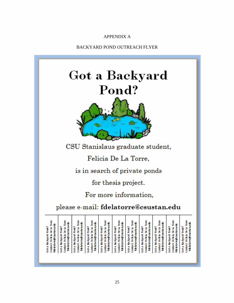
of-mouth and by posting flyers (Appendix A) at local coffee shops, cafés, pet stores, feed stores,
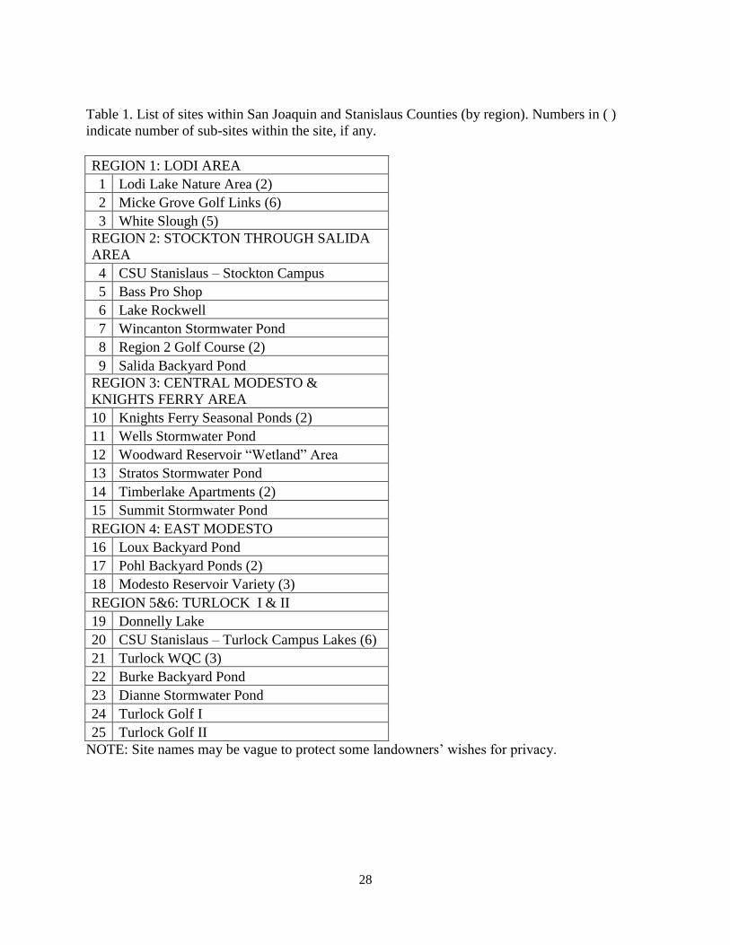
etc. Sites were regionalized to determine which would be feasible to travel to and between,
especially for the time-restrained night surveys (Table 1). Initial contact with land owners and
managers was attempted via e-mail or phone call to discuss what the project entailed.
Once permissions were granted by city, county, and/or department officials, site locations
near permitted areas were targeted in order to create clustered regions of sites. Sites were also
categorized (i.e. urban, suburban, rural) and tallied in order to be sure to have enough
experimental units. Access was granted to approximately 90 water bodies within San Joaquin
County and Stanislaus County of California. Realistically, in order to be able to handle and
sufficiently monitor sites, the list was filtered down to a maximum of 40 sites. An arbitrary
minimum of 20 sites was set in order to gather enough data for statistical significance. As sites
were grouped and routed, some remote sites were removed from the list; these sites would have
required excessive travel time and reduced the number of total sites that could be sampled. Other
site features that were taken into consideration for inclusion in the project were: site safety
(especially during evening hours), access to perimeter of the water body, and hydroperiod (how
long water body holds water throughout the season).
In San Joaquin County, the main cities represented were: Ripon, Manteca, Stockton, and
Lodi. In Stanislaus County, the main cities were: Modesto, Salida, Turlock, and Oakdale.
11
Initially, natural waterways, such as lentic parts (e.g. pools) along the San Joaquin River and
Stanislaus River, were sought to be included in the project, but due to liability and safety issues,
these were excluded for the most part (with the exception of seasonal ponds at Knights Ferry
Recreation Area). The final number of sites totaled 25 with 48 sub-sites (or individual ponds)
contained within them (Table 1).
Timing of Surveys
Starting mid-February 2013, temperature and precipitation in the Stockton Metro Area
and Modesto City/Harry Sham Field Area was monitored daily via local airport weather reports
(National Weather Service. 2013. Available from http://www.weather.gov [Accessed 9 June
2013]). This was important in determining start time for night surveys because migration and
breeding for many amphibians is cued by air temperature and precipitation. After a few rains and
when air temperature has averaged above 18°C (or 65°F), this will cue the start of the breeding
season (Heyer et al. 1994). In San Joaquin and Stanislaus Counties, these conditions typically
occur in early March through April (The Old Farmer’s Almanac. 2013. Available from
http://www.almanac.com/weather/history [Accessed 9 June 2013]). Surveys began on March 5th
,
2013 and continued through May 26th
, 2013.
Amphibian Surveys
Herpetological data used in this study were obtained from the Museum of Vertebrate
Zoology (Accessed through the HerpNet2 Portal, www.HerpNet2.org, 2013-06-01). Historical
presence of amphibians within the designated counties (Table 2) was further confirmed through
published literature (e.g. Fisher and Shaffer 1996), species distribution maps (Lannoo 2005), and
the National Amphibian Atlas (USGS. 2012. National Amphibian Atlas 2.2. Available from
http://www.pwrc.usgs.gov:8080/mapserver/naa/ [Accessed 5 June 2013]). Breeding period may
vary between species based on habitat and environmental preference (Lannoo 2005). For
example, wind has been found to play a role on amphibian presence and abundance (Heyer et al.
1994). In addition to weather, temperature, and precipitation being recorded at each site, wind
was rated using the Beaufort Wind Scale (Table 3; Heyer et al. 1994; Morreale and Sullivan
2011).

12
Night surveys began March 5th
, 2013 and continued weekly until April 20th
, 2013 in order
to bracket the majority of the breeding season. Daytime surveys began intermittently mid-March
and then continued on a case-by-case basis through May 26th
, 2013. Each site was visited a
minimum of two times to observe for initial amphibian presence (unless it was found to be dry
by the second visit, in which case it was visited only once) and a maximum of ten times
(depending on activity). Since aquatic habitats were the primary focal areas of the study,
terrestrial amphibian breeders may have been missed or underrepresented.
Breeding Adults. – Most anurans have unique courtship calls that are made during their
breeding season. These vocalizations are typically projected from males, but in some cases,
especially in areas of high environmental noise, some males will not call (satellite males). While
some may call during the day, the species that are known to be found in San Joaquin County and
Stanislaus County call primarily at night (California Frog and Toad Calls. 2012. California
Herps. Available from http://californiaherps.com [Accessed 9 June 2013]). Site visitations were
scheduled within a half hour after sunset (i.e. when the sun is completely absent). Daily start
times were based on forecast time of sunset.
The first step for night surveys was to perform a three minute auditory survey at the
shoreline of the water body. For this, observers sat and listened for any frog calls and
approximated the number of individuals calling. If number of individuals were too difficult to
distinguish, a call intensity index was used to approximate the number heard (Morreale and
Sullivan 2011).
Next, visual encounter surveys (VES) were implemented by walking the perimeter of the
water body to look for presence of amphibians and any pairs in amplexus. If water body
perimeter at a given site was over 400 meters long, the site was split into two or three transects;
each visit, only part of the perimeter was surveyed, with the individual transects interchanged
each date. Total abundance per length was also observed and recorded.
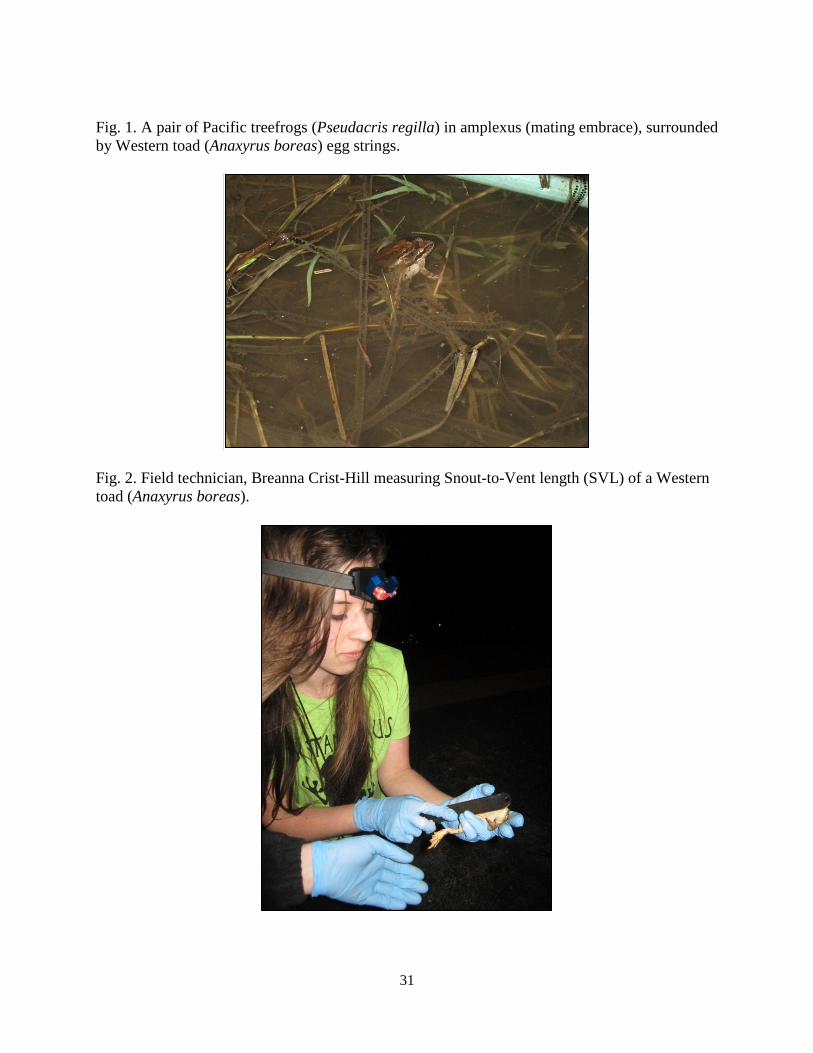
Once presence was established, standard morphological measurements were taken for a
maximum of twenty individuals of each species at each site during a follow-up night survey.
These measurements included: snout-to-vent length (SVL) in millimeters using a ruler (Fig. 2),
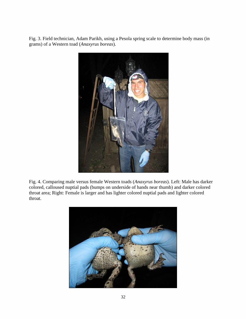
body mass (g) using Pesola spring scales with an attached pre-weighed Ziplock bag of
appropriate size (Fig. 3), and if possible, sex and age category based on features such as: overall
13
body size, nuptial (thumb) pad size and color, and throat color and texture (Stebbins 2003; Fig.
4).
Night survey duration ranged from 10 minutes to two and a half hours to complete, with
an average of half an hour per site (excluding travel time) depending on the size of the water
body and amphibian presence. Originally, I anticipated visiting five or six sites per night, but
both the surveys and the cleaning of materials took longer than expected, resulting in a typical
survey night of one to three sites on average. As stated earlier, sites were grouped into regions
based on proximity. For the initial visits, regions were randomized. Thereafter, all site visitations
were scheduled based on if/which amphibian species were observed (i.e. prioritized by high,
medium, and low) and only time of visit was randomized for the sites in the region. Day surveys
were a little more timely due to the fact that the water quality testing were dependent on sit, wait,
and analysis times, and took an average of one to two hours.
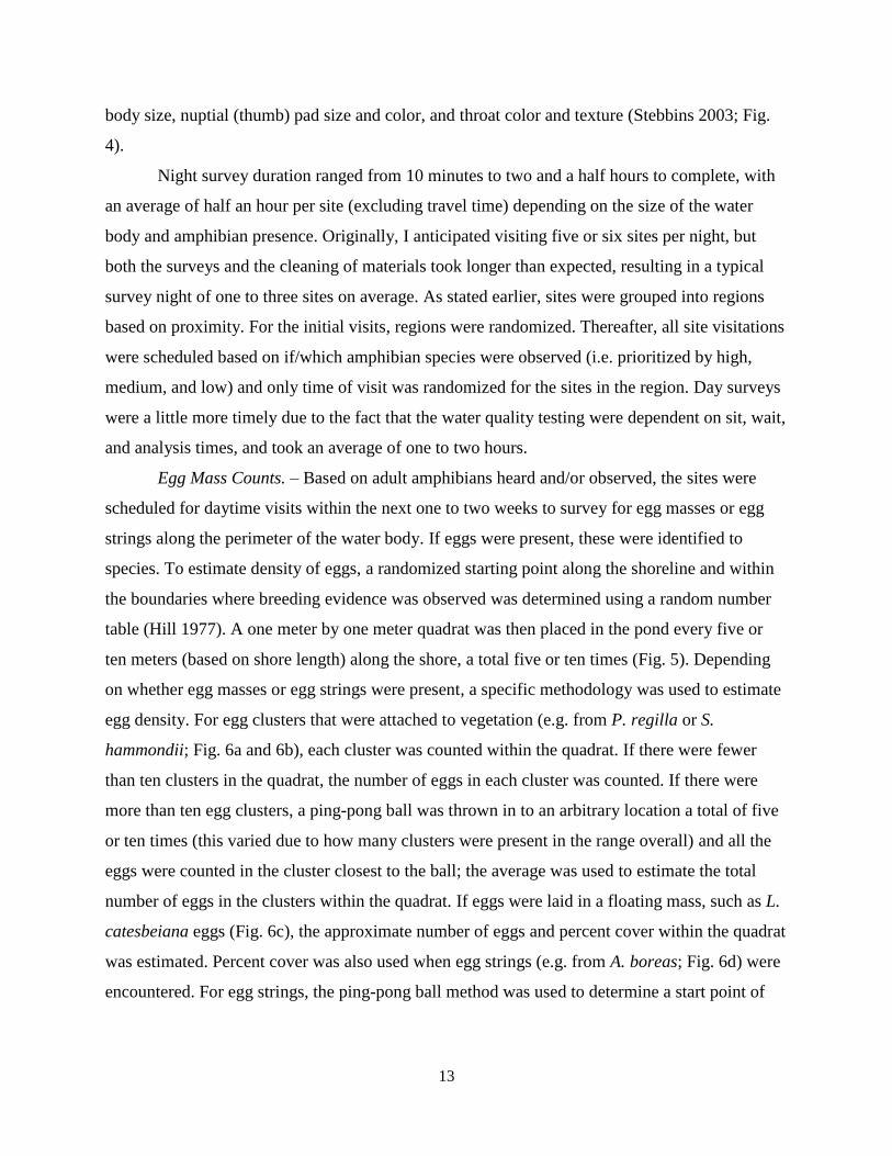
Egg Mass Counts. – Based on adult amphibians heard and/or observed, the sites were
scheduled for daytime visits within the next one to two weeks to survey for egg masses or egg
strings along the perimeter of the water body. If eggs were present, these were identified to
species. To estimate density of eggs, a randomized starting point along the shoreline and within
the boundaries where breeding evidence was observed was determined using a random number
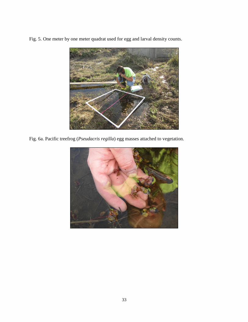
table (Hill 1977). A one meter by one meter quadrat was then placed in the pond every five or
ten meters (based on shore length) along the shore, a total five or ten times (Fig. 5). Depending
on whether egg masses or egg strings were present, a specific methodology was used to estimate
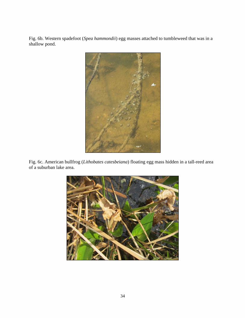
egg density. For egg clusters that were attached to vegetation (e.g. from P. regilla or S.
hammondii; Fig. 6a and 6b), each cluster was counted within the quadrat. If there were fewer
than ten clusters in the quadrat, the number of eggs in each cluster was counted. If there were
more than ten egg clusters, a ping-pong ball was thrown in to an arbitrary location a total of five
or ten times (this varied due to how many clusters were present in the range overall) and all the
eggs were counted in the cluster closest to the ball; the average was used to estimate the total
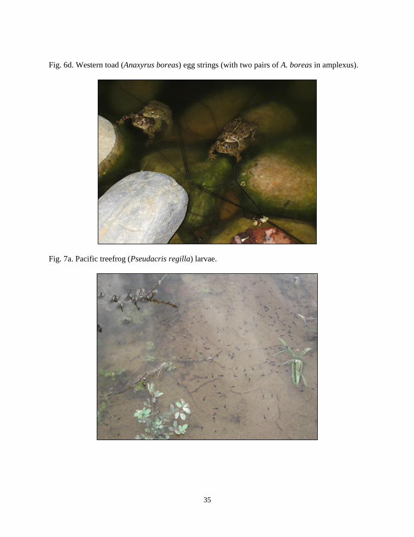
number of eggs in the clusters within the quadrat. If eggs were laid in a floating mass, such as L.
catesbeiana eggs (Fig. 6c), the approximate number of eggs and percent cover within the quadrat
was estimated. Percent cover was also used when egg strings (e.g. from A. boreas; Fig. 6d) were
encountered. For egg strings, the ping-pong ball method was used to determine a start point of

14
where to count within a two centimeter (cm) section. This was repeated five or ten times and the
average was used to estimate the total number of eggs.
Larval Success. – Time to hatching varies by species, but based on eggs present, the sites
were visited over the following weeks to determine presence and approximate density of larvae
(Fig. 7a, 7b, and 7c). Pacific Treefrog (Pseudacris regilla) eggs can take about 2-3 weeks to
hatch (Lannoo 2005), thus these sites were checked less frequently within the time frame. Larval
presence served as an indicator of breeding success.
Potential Predator Surveys
All observations of potential predators, predator fecal matter, or tracks within the study
site areas were also noted.
Voucher Specimens
A maximum of two individuals of each amphibian species not included on the SSC list
(Special Animals List 2011; Table 2) were permitted to be collected from each site if
owner/manager permission was given and to fill museum collection gaps. These collection
limitations excluded American bullfrogs (Lithobates catesbeiana), which are non-native and
whose removal is encouraged.
Collected individuals were humanely euthanized and preserved as voucher specimens
using methods from Simmons (2002). Liver tissue or a toe clipping was also preserved for each
specimen. Vouchers have been deposited at the Museum of Vertebrate Zoology at the University
of California, Berkeley (Fig. 8).
Habitat Variables
Pond Age. – Pond age information is currently being obtained either by communication
with the landowners (if known), by studying historic maps, or by assessing and estimating age
based on vegetative growth. Pond age will be classified after Ostergaard et al. (2008) with < 2.5
years of age categorized as “young”, 2.5 to 7.5 years of age being “intermediate”, and > 7.5 years
of age being “old”.
Aquatic Habitat. – At each visit, basic water quality measurements were recorded as
follows: water temperature, pH, water color, and subsurface visibility. During daytime surveys,

15
the same water quality measurements were assessed, in addition to these: turbidity, dissolved
oxygen (using both a probe and the Winkler Method [Hach Company 2006]), conductivity,
nitrate level, phosphate level. Other notable information included: water depth (if possible at two
meters from shore), shoreline grade, shoreline material, pond liner material, and any other
features that may have affected the aquatic habitat (e.g. decorative fountains on, algae, distinct
odors, etc.). Length, width, perimeter, and surface area of the water bodies were measured using
Google Earth (Google Earth. 2012. Op. cit.). If a water body was too small to observe from
satellite imagery (e.g. backyard pond), then during a daytime visit, a measuring tape was used to
measure length and width of the pond with perimeter and surface area being mathematically
estimated.
Landscape – Migratory amphibians are especially dependent on forested uplands; thus,
characteristics of the surrounding landscape have also been tied to their usage of ponds as
breeding sites (Egan and Paton 2008; Windmiller et al. 2008). I used a qualitative ranking scale
of 0-4 (ranked from none through widely found, respectively) to rate vegetation, shade, and
amount of cover objects available both within the water and on the immediate shore (within 10
meters; Fig. 9a, 9b, and 9c).
Data Analysis
Standard parametric and eco-statistical approaches will be implemented when possible in
order to interpret the data. Statistical programs such as Piface v.1.76, Ecological Methodology
7.0, and Ecosim700, will be used to perform analyses. While post hoc methods are recommended
to determine power (Heyer et al. 1994), these will only be used for habitat variables and diversity
indices. To quantify diversity (i.e. to measure heterogeneity), rarefaction may be used to
determine species richness and PIE Hurlbert’s Index may be used to determine species eveness
(Krebs 1999).
In order to meet my first objective of determining species abundances, I will use a one-
way ANOVA to explain variations in the abundance counts of species within and between site
types. In this analysis, abundance will be estimated by number of frogs/m2 for each pond. Sites
without amphibian species presence will not be included. Assuming that mean abundance at
urban sites will be the least (e.g. 1-5 frogs/m2), semi-urban sites intermediate (e.g. 5.1-10
frogs/m2), and rural sites highest (e.g. >10.1 frogs/m
2), the p-value will show if results are
16
significantly different across sites based on these expected values. Chi-squared analysis using
proportions will also be used to test for differences in the proportion of individuals of different
species between sites. This will include looking at presence and absence, as well as sex rations
within and between site types and individual sites.
For my second objective, in order to determine which habitat characteristics drive species
distributions, either Principal Components Analysis (PCA) or Non-metric Multidimensional
Scaling (NMS) will be used via the PC-ORD statistical program. These analyses are used to
determine the percent of each contributing factor within the habitat or environment. Egan and
Paton (2008) used PCA in their study of pond-breeding amphibians across a rural-urban gradient.
In this study, within-pond characteristics, such as hydroperiod and percent cover by aquatic
vegetation, were shown to be associated with egg mass counts. With PCA, the variables are
combined on a principle axis and variance is explained for each characteristic. EcoSim700 null
models can be tested to observe for co-occurrence within a presence-absence matrix. Non-metric
Multidimensional Scaling is a newer approach that can differentiate factor influence on a
dependent variable and is very similar to PCA.
My third objective will be met by determining the succession of the number of eggs
(approximated from egg mass counts or percent cover) to the abundance of larvae that are
estimated during the follow-up surveys for each site. This will represent overall percentage of
breeding success for each species and at each site.
For my final objective, I will use a one-way ANOVA to determine effects of predators on
urban and suburban amphibian species. This will include comparing abundance of predators to
the abundance of amphibians and egg masses. To determine if mean species diversity differs
with presence of American bullfrog (Lithobates catesbeiana) a two-tailed Student’s t-test will be
used, employing an α ≤ 0.05 (Ostergaard et al. 2008).
Other considerations –Multiple ponds within a given area (e.g Timberlake apartment
complex) will be designated as sub-sites. If ponds were within 500 meters of each other and can
potentially have intermixing populations, data will be analyzed separately as well as combined
overall as a site to avoid pseudoreplication (Ostergaard et al. 2008).

17
PROJECT OUTCOMES
Amphibian Abundance
Total number of amphibians observed and/or heard was about 250 individuals. Sites
ranged from having no individuals to over 100 individuals. Out of the 25 sites, only four did not
have any evidence of amphibian presence.
Amphibian Species Richness
Out of the historical list of amphibian species found within Stanislaus and San Joaquin
Counties (Table 2), the common species were found as expected (e.g. Pseudacris regilla
complex [Fig. 10a] and Anaxyrus boreas [Fig. 10b]). Lithobates catesbeiana (Fig. 10c) was also
found as expected and was included in the biodiversity count, but since this is an invasive
species, they may have hindered areas from gaining other potential species. One surprising find,
because they have not been scientifically documented in these counties for over a decade, was
the western spadefoot (Spea hammondii [Fig. 10d]). Out of all the amphibian species that were
found, the most common species was P. regilla (found at 14 sites) and the least common was S.
hammondii (found at only two sites; Fig. 11).
Amphibian Breeding Success
While 84% of the ponds showed presence of at least one amphibian species, this did not
necessarily indicate breeding success. Breeding success was determined at each site by
calculating the percentage as to which breeding attempts were made, as follows: 0% Breeding
Success = No presence or presence of only one amphibian individual; 20% Breeding Potential=
Presence of at least 2 individuals, no calling or observations of amplexus; 40% Breeding
Attempts= Presence of at least 2 individuals heard calling and/or amplexus observed; 60%
Breeding Success= Egg clusters or strings observed; 80% Breeding Success= Larvae hatched
from eggs; 100% Breeding and Developmental Success= Metamorphs/froglets observed
Five sites had 0% breeding attempts. Five sites had 100% breeding success observed or
confirmed by landowner (Fig. 12): Salida backyard pond, Knights Ferry ponds, Timberlake
apartment ponds, Modesto reservoir (sub-site), and Wincanton stormwater pond. This could have
been an underestimate because the two sites that had larvae present could have just been delayed
on metamorphosis time and/or I was not able to make it back for another follow-up visit. At the

18
Wincanton stormwater pond, one lone toadlet was found, even though egg strings were never
observed. It is possible that I failed to note egg strings due to the fact that the shoreline was very
steep; it was tough to walk the perimeter at most of the site. For the most part, we walked about
20 feet above the water on a walkway and attempted to look for any toads that have traveled up
or were on their way down. We only went close to the shoreline at the ends of the pond that had
ramps.
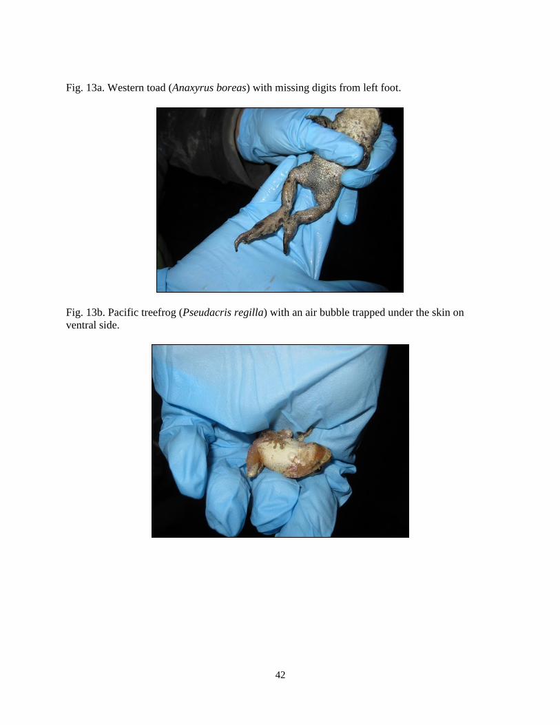
Amphibian Deformities
Since the 1990’s, amphibian deformities have been a topic of concern. It has been said
that a typical amphibian population has an abnormality prevalence of 3.3% (95% CI: 3.0-3.6%)
(Lunde and Johnson 2012). This means that for every 100 amphibians captures, about 3 will
have some sort of deformity. Since I had such low capture rates at my sites and I only did visual
field-based inspections, I was not able to detect abnormality rates. I did run across three
individuals at three different sites that had interesting morphological characteristics. One of these
was a Western toad discovered with his left foot digits tapered off like a paintbrush (Fig. 13a).
Another was a Pacific treefrog with what looked like an air bubble trapped under his skin on his
upper ventral area (Fig. 13b). Lastly, there was an American bullfrog individual had a small
calloused bump on his head (no photograph).
Potential Predators and Other Wildlife
When dealing with water bodies, especially those that are stagnant, mosquitos become an
issue of concern. Mosquitofish (Gambusia affinis [Fig. 14a]) are often introduced in order to
control the mosquito population (California’s Central Valley. 2006. Just the Facts, Public Policy
Institute of California. Available from http://www.sjmosquito.org/about-us/welcome.htm
[Accessed 30 June 2013]). Sixteen out of 25 sites had presence of fish and of these, nine had
mosquitofish. While fish presence did not completely deter amphibian presence, amphibian
breeding success was especially lacking at these sites/sub-sites, possibly due to the fact that fish
feed on amphibian eggs. Mosquitofish especially will eat anything that they can fit in their
mouths (OFDW Backgrounder 2009).

19
Another group of prevalent potential predators were geese, ducks, and other medium to
large size waterfowl. Some other potential predators consisted of racoons, feral cats, skunks, and
dogs (especially for backyard ponds).
American bullfrogs were present at 12 of the sites. While these are amphibians, they are
non-native invasives and their harmful effects on native wildlife are well-documented (McCoid
1995; Rosen and Schwalbe 1995). American bullfrogs feast on eggs, larvae, and adults of other
species of amphibians and even their own (Lithobates catesbeianus – American bullfrog.
California Herps. Available from http://www.californiaherps.com/frogs/pages/r.catesbeiana.html
[Accessed 30 June 2013]). It is interesting that eight of the nine sites that contained mosquitofish
also contained American bullfrogs. This brings up another topic that can lead to further evidence
that non-native species may actually help other invaders thrive, such as with the symbiosis
between beach grass and deer mice in Marin County, California (Mirsky, S. 2010. Invasive
Species Lets Other Species Disrupt Environment. Scientific American. Available from
http://www.scientificamerican.com/podcast/episode.cfm?id=invasive-species-lets-other-species-
10-08-16 [Accessed 1 July 2013]).
Other intriguing wildlife that we came across included: a beaver at one of the more
natural sites, White Slough (most likely a non-predator, but definitely a habitat engineer; Fig.
14b). I also spotted a Texas softshell turtle (Fig. 14c).
Habitat Variables and Water Quality
Most amphibians (at least in the United States) require water at least 15 cm deep, in order
to breed (Richter 1997; Ostergaard et al. 2008). At the sites that I observed, water depth ranged
from about 5 cm to approximately 80 cm (within one to two meters from the shoreline, if
possible). Even at the sites with less than 15 cm, amphibians were utilizing the area and
breeding. One of the backyard ponds located in Salida had about 6 cm of standing water and was
supporting a handful of breeding Western toads and Pacific treefrogs!
In terms of within pond and surrounding vegetation, this seemed to vary by site and even
sub-site. Areas that were not intended for public use (e.g. stormwater ponds, water treatment
plants) seemed to have fewer ornamentals shrubs and tree growth. It is important to note that
trees can act as a natural barrier to run-off of pollutants and should be incorporated for
landscaping around any water body regardless of purpose.
20
Water quality measurements varied by site and even within a single site by date in some
cases. Conductivity, turbidity, and pH levels were pretty standard and did not vary significantly
beyond expected ranges. The most surprising results were that all but four sub-sites had traces of
nitrates and phosphates, which are common by-products that are produced from fertilizers,
pesticides, and ammonia products. Even the natural, remote areas that were used as control sites
had a small amount of either nitrate/phosphate contamination. The highest level of nitrates was
found at the Dianne stormwater pond (yet this still drew a lot of amphibian activity, namely
Western spadefoots and Western toads). The highest level of phosphates was found at one of the
water bodies at the White Slough Water Pollution Control Facility (but it still did not deter a
couple of Pacific treefrogs and an American bullfrog from visiting the area).
Another water quality test that was done was to determine the level of dissolved Oxygen
(DO). DO is an important component in all aquatic ecosystems because it provides energy for the
organisms that live within. DO levels change throughout the day and are inversely related to the
water and environmental temperature. Thus, at higher temperatures, DO will be low. DO levels
that are too low can leave water to be hypoxic, or with little or no oxygen. Studies have shown
that a normal pond would have a DO level of about 5-6 ppm (Sinclair 2007; Water’s the Matter.
Available from http://peer.tamu.edu/curriculum_modules/water_quality/module_3/lesson4.htm
[Accessed 10 July 2013]).
Two methods were used: a DO meter probe and a titration method (also known as the
Winkler Method). Since the DO meter probe did not cooperate each time and seemed to be
overly sensitive, I decided to just use the Winkler method as the reliable results of measure. DO
Values ranged from a low of 2.6 mg/L (Modesto backyard pond) to a high of 15 mg/L (Donnelly
Park). The backyard pond with the lowest DO level had a group of goldfish and sightings of a
pair of Western toads, thus this shows the DO was still high enough to avoid hypoxia. The low
level could have been due to a large amount of leaf and branch debris that was covering the
bottom of the pond (about 24 cm high) and creating a lot of organic matter. Donnelly Park had
the highest DO level, probably due to the high amount of productivity and large population of
fish, ducks, and geese. High activity can lead to high aeration of the water, so this makes sense.

21
CONCLUSIONS
While breeding success seemed to be low at the selected sites, the evidence of amphibian
presence and breeding attempts demonstrate that urban and suburban ponds are being used
because they provide a moist environment that may be otherwise lacking in the area. They also
may assist in providing connectivity across the landscape and help with creating meta-
populations.
Although my project was for a single season, it can act as a stepping-stone and open the
doors to amphibian studies at other sites within these agriculturally-dominated counties. This
project not only gave me insight into what it is like to be a field biologist, but it helped me gain
skills in leadership, marketing, communication, and community outreach.
I suggest that future studies should be conducted at the sites that I used, especially those
that had even partial breeding success, in order to develop a monitoring program to direct future
management strategies of the water bodies. Furthermore, just because breeding attempts were not
successful during the year of my study does not negate the possibility that breeding success
varies through time. Additional sites should also be sought out (refer to Appendix B), especially
those that are privately-owned and do not typically permit public access, due to the fact that
these areas usually do not have as many external influences (e.g. introduced species from people
releasing pets, people catching amphibians, or people intentionally dumping litter/waste in the
pond) that can affect amphibian populations.
Due to the fact that travel between sites, scheduling, and cleaning of equipment of
materials is time consuming, perhaps the focus could shift to some of the higher activity sites or
perhaps different methodology should be considered (e.g. dip-netting for larvae). Another
suggestion would be to focus on a particular type of site such as looking at golf courses within
one county, or backyard ponds within a sector or at particular distances from source ponds.
Whatever the case, I sincerely hope that my results will provide the baseline data to support
further study and that I have opened doors of opportunity at these sites for future graduate
students that are interested in this field.

22
REFERENCES
Dodd, C.K.J. (Ed.). 2010. Amphibian Ecology and Conservation: A Handbook of Techniques.
Oxford, New York. Pp. 105-117.
Egan, R.S. and P.W.C. Paton. 2008. Multiple scale habitat characteristics of pond-breeding
amphibians across a rural-urban gradient. In J.C. Mitchell, R.E. Jung Brown, and B.
Bartholomew (eds.), Urban Herpetology. Pp. 53-65. Herpetological Conservation vol. 3,
Society for the Study of Amphibians and Reptiles, Salt Lake City, UT.
Fisher, R.N., and H.B. Shaffer. 1996. The decline of amphibians in California’s Great Central
Valley. Conservation Biology 10: 1387-1397.
Hach Company. 2006. Dissolved Oxygen Test: 0.2 to 4 and 1 to 20 mg/L O2, for test kit 146900
(Model OX-2P) edition 1.
Hamer, A.J., and M.J. MacDonnell. 2008. Amphibian ecology and conservation in the
22regarious world: A review. Biological Conservation 141: 2432-2449.
Heyer, W.R., M.A Donnelly, R.W. McDiarmid, , L.C. Hayek, and M.S. Foster (Eds.). 1994.
Measuring and Monitoring Biological Diversity: Standard Methods for Amphibians.
Smithsonian Institution Press, Washington, DC.
Hill, A.B. 1977. A Short Textbook of Medical Statistics. Hodder and Stoughton, London.
Krebs, C.J. 1999. Ecological Methodology, second ed. Addison-Welsey Educational Publishers,
Inc.
Lannoo, M. (Ed.). 2005. Amphibian Declines: The Conservation Status of United States Species.
University of California Press, Ltd., Berkeley and Los Angeles, CA.
Lunde, K.B. and P.T.J. Johnson. 2012. A practical guide for the study of malformed amphibians
and their causes. Journal of Herpetology 46: 429-441.
McCoid, M. J. 1995. Non-native reptiles and amphibians. Pages 433-437 in Laroe, E. T., G. S.
Farris, C. E. Puckett, P. D. Doran, and M. J. Mac, editors. Our living resources: a report
to the nation on the distribution, abundance, and health of U.S. plants, animals, and
ecosystems. U.S. Department of the Interior, National Biological Service, Washington,
D.C. 530 p.
Morreale, S.J. and K.L. Sullivan. 2011. Frog Call Survey Protocol. E.L. Rose Conservancy.
Cornell Department of Natural Resources.
OFDW Backgrounder: Using Mosquitofish (Gambusia Affinis) for Mosquito Control. 2009.
Oregon Department of Fish and Wildlife.
23
Ostergaard, E.C., K.O. Richter, and S.D. West. 2008. Amphibian use of stormwater ponds in the
Puget lowlands of Washington, USA. In J.C. Mitchell, R.E. Jung Brown, and B.
Bartholomew (eds.), Urban Herpetology. Pp. 259-270. Herpetological Conservation vol.
3, Society for the Study of Amphibians and Reptiles, Salt Lake City, UT.
Richter, K.O. 1997. Criteria for the restoration and creation of wetland habitats of lentic-
breeding amphibians of the Pacific Northwest. In K.B.Macdonald and F. Weinmann
(eds.), Wetland and Riparian Restoration: Taking a Broader View. Pp.72-94. USEPA,
Region 10, Seattle, WA.
Rosen, P. C. and C. R. Schwalbe. 1995. Bullfrogs: introduced predators in southwestern
wetlands. Pages 452-454 in Laroe, E. T., G. S. Farris, C. E. Puckett, P. D. Doran, and M.
J. Mac, editors. Our living resources: a report to the nation on the distribution,
abundance, and health of U.S. plants, animals, and ecosystems. U.S. Department of the
Interior, National Biological Service, Washington, D.C. 530 p
Simmons, J.E. Herpetological Collecting and Collections Management, Revised Edition. 2002.
Vi, 153 pp. Paperback.
Sinclair, H. 2007. A comparative study of amphibian populations in agricultural and non-
agricultural aquatic ecosystems.
Umbach, K.W. 1997. A Statistical Tour of California’s Great Central Valley. California
Research Bureau. California State Library.
Vitt, L.J. and J.P. Caldwell. 2009. Herpetology, third ed. Elsevier Inc.: Burlington, MA
Windmiller, B., R.N. Homan, J.V. Regosin, L.A. Willitts, D.L. Wells, and J.M. Reed. 2008.
Breeding amphibian population decline following loss of upland forest habitat around
vernal pools in Massachusetts, USA. In J.C. Mitchell, R.E. Jung Brown, and B.
Bartholomew (eds.), Urban Herpetology. Pp. 41-51. Herpetological Conservation vol. 3,
Society for the Study of Amphibians and Reptiles, Salt Lake City, UT.

APPENDICES
25
APPENDIX A
BACKYARD POND OUTREACH FLYER

26
APPENDIX B
OTHER SITES (NOT INCLUDED IN THIS PROJECT)
WITH EVIDENCE OF AMPHIBIAN BREEDING ATTEMPTS
Various irrigation canals where P. regilla were heard calling from (in Modesto, CA and
Riverbank, CA)
Agricultural fields with sightings of salamanders (per word of mouth)
Agricultural fields surrounding some of the sites included in this project (e.g. Turlock,
CA and Modesto, CA)
Backyard pond in Patterson, CA (CW)
Backyard pond in Stockton, CA (DW)
Backyard pond in Turlock, CA (DM)
Backyard pond in Modesto, CA (JH)
Backyard pond in Lodi, CA (KH)
Front yard pond in Modesto, CA (TT)
Backyard without pond, but occasionally floods and draws A. boreas (MC)
Escalon Creative Water Gardens
Modesto Secondary Wastewater Facility
Stormwater ponds in Linden, CA
Park and Trail near Eight Mile Road (Stockton, CA)
Micke Grove Park (Lodi, CA)

27
TABLES
28
Table 1. List of sites within San Joaquin and Stanislaus Counties (by region). Numbers in ( )
indicate number of sub-sites within the site, if any.
REGION 1: LODI AREA
1 Lodi Lake Nature Area (2)
2 Micke Grove Golf Links (6)
3 White Slough (5)
REGION 2: STOCKTON THROUGH SALIDA
AREA
4 CSU Stanislaus – Stockton Campus
5 Bass Pro Shop
6 Lake Rockwell
7 Wincanton Stormwater Pond
8 Region 2 Golf Course (2)
9 Salida Backyard Pond
REGION 3: CENTRAL MODESTO &
KNIGHTS FERRY AREA
10 Knights Ferry Seasonal Ponds (2)
11 Wells Stormwater Pond
12 Woodward Reservoir “Wetland” Area
13 Stratos Stormwater Pond
14 Timberlake Apartments (2)
15 Summit Stormwater Pond
REGION 4: EAST MODESTO
16 Loux Backyard Pond
17 Pohl Backyard Ponds (2)
18 Modesto Reservoir Variety (3)
REGION 5&6: TURLOCK I & II
19 Donnelly Lake
20 CSU Stanislaus – Turlock Campus Lakes (6)
21 Turlock WQC (3)
22 Burke Backyard Pond
23 Dianne Stormwater Pond
24 Turlock Golf I
25 Turlock Golf II
NOTE: Site names may be vague to protect some landowners’ wishes for privacy.
29
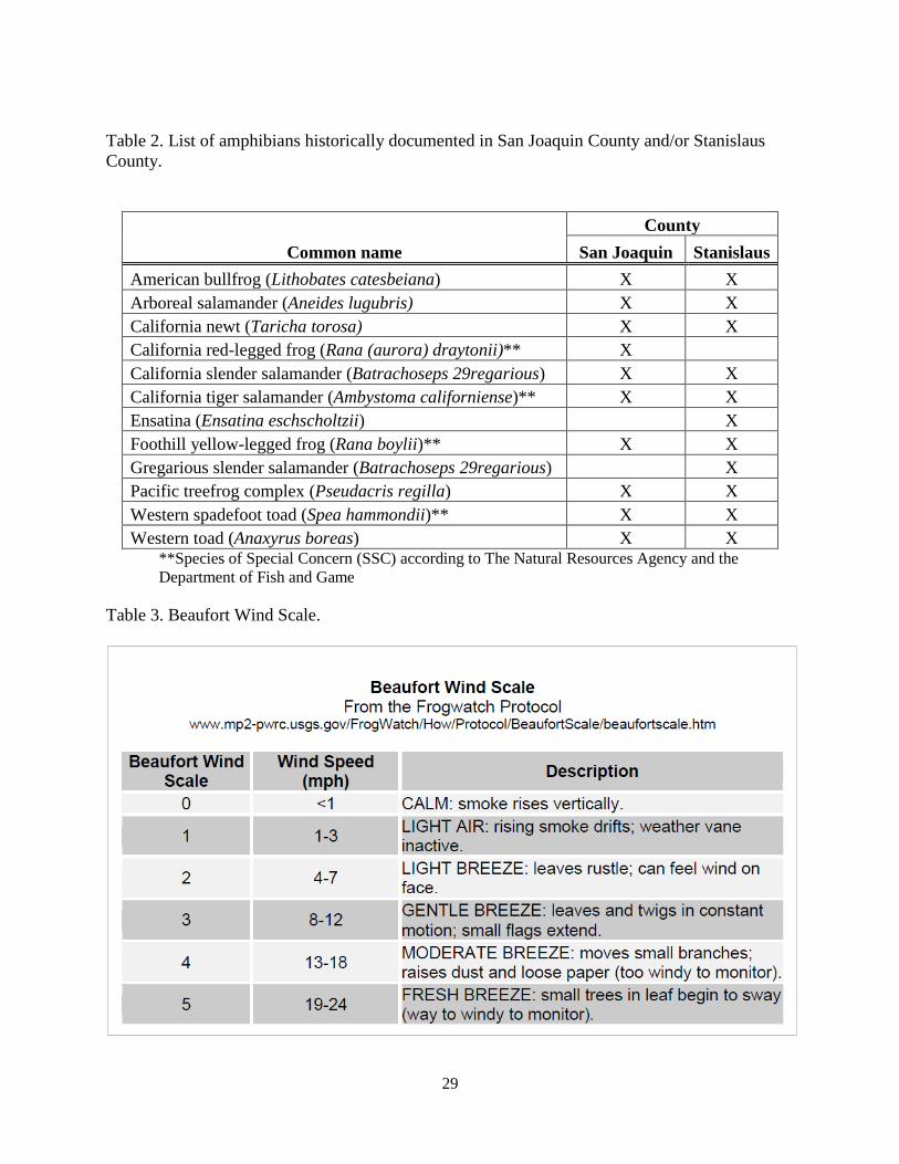
Table 2. List of amphibians historically documented in San Joaquin County and/or Stanislaus
County.
Common name
County
San Joaquin Stanislaus
American bullfrog (Lithobates catesbeiana) X X
Arboreal salamander (Aneides lugubris) X X
California newt (Taricha torosa) X X
California red-legged frog (Rana (aurora) draytonii)** X
California slender salamander (Batrachoseps 29regarious) X X
California tiger salamander (Ambystoma californiense)** X X
Ensatina (Ensatina eschscholtzii)
X
Foothill yellow-legged frog (Rana boylii)** X X
Gregarious slender salamander (Batrachoseps 29regarious) X
Pacific treefrog complex (Pseudacris regilla) X X
Western spadefoot toad (Spea hammondii)** X X
Western toad (Anaxyrus boreas) X X **Species of Special Concern (SSC) according to The Natural Resources Agency and the
Department of Fish and Game
Table 3. Beaufort Wind Scale.

30
FIGURES
31
Fig. 1. A pair of Pacific treefrogs (Pseudacris regilla) in amplexus (mating embrace), surrounded
by Western toad (Anaxyrus boreas) egg strings.
Fig. 2. Field technician, Breanna Crist-Hill measuring Snout-to-Vent length (SVL) of a Western
toad (Anaxyrus boreas).
32
Fig. 3. Field technician, Adam Parikh, using a Pesola spring scale to determine body mass (in
grams) of a Western toad (Anaxyrus boreas).
Fig. 4. Comparing male versus female Western toads (Anaxyrus boreas). Left: Male has darker
colored, calloused nuptial pads (bumps on underside of hands near thumb) and darker colored
throat area; Right: Female is larger and has lighter colored nuptial pads and lighter colored
throat.
33
Fig. 5. One meter by one meter quadrat used for egg and larval density counts.
Fig. 6a. Pacific treefrog (Pseudacris regilla) egg masses attached to vegetation.
34
Fig. 6b. Western spadefoot (Spea hammondii) egg masses attached to tumbleweed that was in a
shallow pond.
Fig. 6c. American bullfrog (Lithobates catesbeiana) floating egg mass hidden in a tall-reed area
of a suburban lake area.
35
Fig. 6d. Western toad (Anaxyrus boreas) egg strings (with two pairs of A. boreas in amplexus).
Fig. 7a. Pacific treefrog (Pseudacris regilla) larvae.
36
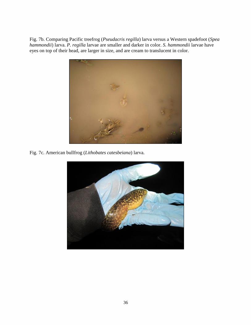
Fig. 7b. Comparing Pacific treefrog (Pseudacris regilla) larva versus a Western spadefoot (Spea
hammondii) larva. P. regilla larvae are smaller and darker in color. S. hammondii larvae have
eyes on top of their head, are larger in size, and are cream to translucent in color.
Fig. 7c. American bullfrog (Lithobates catesbeiana) larva.

37
Fig. 8. Graduate student, Felicia De La Torre, with the voucher specimens at UC Berkeley
Museum of Vertebrate Zoology.
Fig. 9a. Knights Ferry seasonal ponds.

38
Fig. 9b. A couple of stormwater ponds in Stanislaus County: Summit stormwater pond (Modesto,
CA) and Wincanton stormwater pond (Salida, CA).
Fig
Fig. 9c. A couple of ornamental ponds/lakes: Pohl Backyard Pond and CSU Stanislaus -
Stockton Lake.

39
Fig. 10a. Pacific treefrog (Pseudacris regilla) adult.
g. 10b. Western Toad (Anaxyrus boreas) adult.
40
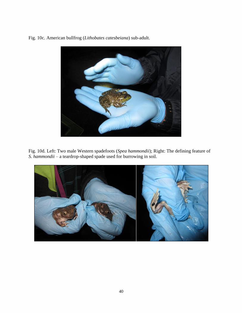
Fig. 10c. American bullfrog (Lithobates catesbeiana) sub-adult.
Fig. 10d. Left: Two male Western spadefoots (Spea hammondii); Right: The defining feature of
S. hammondii – a teardrop-shaped spade used for burrowing in soil.

41
Fig. 11. Number of sites with indicated amphibian species.
Fig. 12. Number of sites with the breeding success rate as indicated.
0
2
4
6
8
10
12
14
16
Spea hammondii Anaxyrus boreas Lithobates catesbeiana Pseudacris regilla
# o
f S
ites
Species
Amphibian Species vs. # of Sites
0
1
2
3
4
5
6
7
8
9
0% Breeding
Success
20% Breeding
Potential
40% Breeding
Attempts
60% Breeding
Success
80% Breeding
Success
100% Breeding
Success
# o
f S
ites
Breeding Success Rate
Breeding Success Rate vs. # of Sites
42
Fig. 13a. Western toad (Anaxyrus boreas) with missing digits from left foot.
Fig. 13b. Pacific treefrog (Pseudacris regilla) with an air bubble trapped under the skin on
ventral side.

43
Fig. 14a. Mosquitofish (Gambusia affinis) are prevalent in urban and suburban aquatic
ecosystems. (Stock photo from: www.sccgov.org )
Fig. 14b. North American Beaver (Castor Canadensis) at White Slough.

44
Fig. 14c. Texas softshell turtle (Apalone spinifera) at Donnelly Park.
Fig. 15. Frog team miniature golf outing. From left to right, (front): Dr. Marina Gerson, Alison
Loux, Felicia De La Torre, Michelle Lopez, Yolanda De La Torre; (back): Sandy Pohl, Loren
Pohl, Jacob Pohl.*
*Missing from photo: Kelly Baker, Esther Buie, Paul Coates, Mitchell Court, Breanna Crist-Hill, Rick De
La Torre, Elizabeth Grolle, Adam Parikh, Nicole Siemens, and Felisha Walls.


