

Bioinformatics
Xu GuBioinformatics Research Centre
www.brc.dcs.gla.ac.ukDepartment of Computing Science, University of Glasgow
Modelling dynamicbehaviour
(Systems biology)

(c) David Gilbert, Xu Gu 2008 Modelling dynamic behaviour 2
Lecture outline• Biochemical reactions• Modelling with Ordinary Differential Equations• Kinetics : Mass Action• Examples
– Signalling & metabolic pathways– Trypanothione metabolism in Trypanosoma brucei– Oscillators & Amplifiers
• Analysis• ODE simulators

(c) David Gilbert, Xu Gu 2008 Modelling dynamic behaviour 3
What is modelling?
• In this context:
– Translating a biological pathway into mathematics for subsequent analysis
A Bk1
k2
Translating a biologicalpathway
][][][
][][][
21
21
BkAkdt
Bd
BkAkdt
Ad
!=
+!=
[A] = 10; [B] = 0; k1 = 2; k2 = 1; Time = 10
Into mathematics For subsequent analysis
Slide fromRichard Orton
(c) David Gilbert, Xu Gu 2008 Modelling dynamic behaviour 4
Why model?• Simplistic answers:
– Because it’s there…– Why not?
• Technical answer:
– “The benefit of formal mathematical models is that they can show whether proposed causal mechanisms are atleast theoretically feasible and can help to suggest experiments that might further discriminate betweenalternatives.” (Franks & Tofts, 1994)
• Realistic answers:
– A computer model can generate new insights– A computer model can make testable predictions– A computer model can test conditions that may be difficult to study in the laboratory– A computer model can rule out particular explanations for an experimental observation– A computer model can help you identify what’s right and wrong with your hypotheses (could/is the proposed
mechanism correct)
Slide fromRichard Orton

(c) David Gilbert, Xu Gu 2008 Modelling dynamic behaviour 5
Why model?
• In a complex pathway, knowing all the proteins involved and what they do, may still not tell you how thepathway works
• Furthermore, if all the initial concentrations and rate constants are known in the pathway, a computersimulation will probably still be needed to show how the system behaves over time
A
B
C
D
E
F G
H
J
I
K
L
M
K1=2
K-3=3
K2=2
K3=1
K4=10K5=5K-5=4
K6=1
K7=3
K8=6
K-8=7
K9=15
[A]=92
[B]=65
[E]=43
[M]=0 [K]=0
[L]=0
[J]=0
[I]=0
[H]=0
[G]=0[F]=0
[D]=0
[C]=0
Slide fromRichard Orton
(c) David Gilbert, Xu Gu 2008 Modelling dynamic behaviour 6
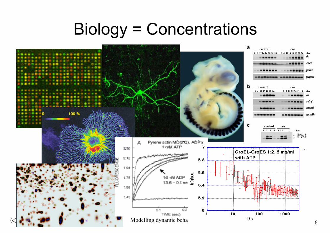
Biology = Concentrations

(c) David Gilbert, Xu Gu 2008 Modelling dynamic behaviour 7
...but biological systems contain
•non-linear interaction between components
• positive and negative feedback loops
• complex cross-talk phenomena

(c) David Gilbert, Xu Gu 2008 Modelling dynamic behaviour 8
The simplest chemical reaction
A B
• irreversible, one-molecule reaction• examples: all sorts of decay processes, e.g. radioactive, fluorescence,
activated receptor returning to inactive state• any metabolic pathway can be described by a combination of processes of
this type (including reversible reactions and, in some respects, multi-molecule reactions)

(c) David Gilbert, Xu Gu 2008 Modelling dynamic behaviour 9
The simplest chemical reaction
A Bvarious levels of description:• homogeneous system, large numbers of molecules = ordinary
differential equations, kinetics• small numbers of molecules = probabilistic equations,
stochastics• spatial heterogeneity = partial differential equations, diffusion• small number of heterogeneously distributed molecules =
single-molecule tracking (e.g. cytoskeleton modelling)

(c) David Gilbert, Xu Gu 2008 Modelling dynamic behaviour 10
Some (Bio)Chemical Conventions
Concentration of Molecule A = [A], usually in units mol/litre(molar)
Rate constant = k, with indices indicating constants for variousreactions (k1, k2...)
Therefore:AB
][][][
1 Akdt
Bd
dt
Ad!=!=

(c) David Gilbert, Xu Gu 2008 Modelling dynamic behaviour 11
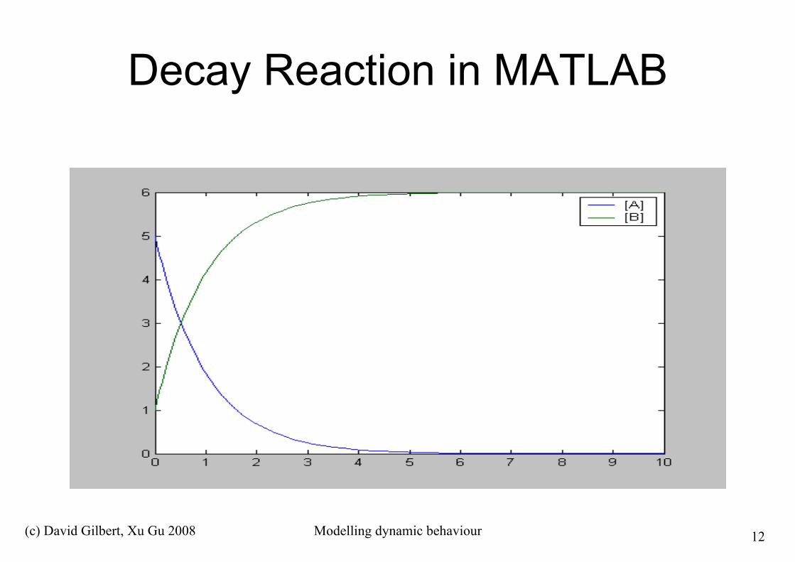
Description in MATLAB:1. Simple Decay Reaction
M-file (description of the model)function dydt = decay(t, y)% A -> B or y(1) -> y(2)k = 1;dydt = [-k*y(1) k*y(1)];Analysis of the model>> [t y] = ode45(@decay, [0 10], [5 1]);>> plot (t, y);>> legend ('[A]', '[B]');
(c) David Gilbert, Xu Gu 2008 Modelling dynamic behaviour 12
Decay Reaction in MATLAB

(c) David Gilbert, Xu Gu 2008 Modelling dynamic behaviour 13
Reversible, Single-MoleculeReaction
A ↔ B, orDifferential equations:
][][][
][][][
21
21
BkAkdt
Bd
BkAkdt
Ad
!=
+!=
forward reverse
Main principle: Partial reactions are independent!
© Rainer Breitling

(c) David Gilbert, Xu Gu 2008 Modelling dynamic behaviour 14
Reversible, single-molecule reaction – 2
Differential Equation:
Equilibrium (=steady-state):
equi
equi
equi
equiequi
equiequi
Kk
k
B
A
BkAk
dt
Bd
dt
Ad
==
=+!
==
1
2
21
][
][
0][][
0][][
][][][
][][][
21
21
BkAkdt
Bd
BkAkdt
Ad
!=
+!=

(c) David Gilbert, Xu Gu 2008 Modelling dynamic behaviour 15
Description in MATLAB:2. Reversible Reaction
M-file (description of the model)function dydt = isomerisation(t, y)% A <-> B or y(1) <-> y(2)k1 = 1;k2 = 0.5;dydt = [-k1*y(1)+k2*y(2) % d[A]/dt k1*y(1)-k2*y(2) % d[B]/dt ];Analysis of the model>> [t y] = ode45(@isomerisation, [0 10], [51]);
>> plot (t, y);>> legend ('[A]', '[B]');

(c) David Gilbert, Xu Gu 2008 Modelling dynamic behaviour 16
Isomerization Reaction in MATLAB

(c) David Gilbert, Xu Gu 2008 Modelling dynamic behaviour 17
Isomerization Reaction in MATLAB
If you know the concentration at onetime, you can calculate it for anyother time... so what would be thealgorithm for that?

(c) David Gilbert, Xu Gu 2008 Modelling dynamic behaviour 18
Euler’s method - pseudocode
1. define f(t,y)2. input t0 and y0.3. input h and the number of steps, n.4. for j from 1 to n do a. m = f(t0,y0) b. y1 = y0 + h*m c. t1 = t0 + h d. Print t1 and y1 e. t0 = t1 f. y0 = y15. end
WhereOne step of Euler’s integration from tn to tn+1 = tn + h is:Yn+1 = yn + hf(tn,yn) where h is the (time) step andf(tn,yn)is the differential equation
),(1 nnnn ythfyy +=+
© Rainer Breitling

(c) David Gilbert, Xu Gu 2008 Modelling dynamic behaviour 19
Improving Euler’s method
)),(,(21
21
1 nnnnnn ythfyhthfyy +++=+
),(1 nnnn ythfyy +=+
(second-order Runge-Kutta method)
© Rainer Breitling

(c) David Gilbert, Xu Gu 2008 Modelling dynamic behaviour 20
Isomerization Reaction in MATLAB

(c) David Gilbert, Xu Gu 2008 Modelling dynamic behaviour 21
Irreversible, two-molecule reaction
A+BCDifferential equations:
]][[][
][][][
BAkdt
Ad
dt
Cd
dt
Bd
dt
Ad
!=
!==
Underlying idea: Reaction probability = Combined probability that both [A]and [B] are in a “reactive mood”:
]][[][][)()()( *
2
*
1 BAkBkAkBpApABp ===
The last piece of the puzzle
Non-linear!

(c) David Gilbert, Xu Gu 2008 Modelling dynamic behaviour 22
Metabolic Networks as Bigraphs
ABC+D
-k3[C][D]+k2[B][D]
-k3[C][D]+k2[B][C]
+k3[C][D]-k2[B]+k1[A][B]
-k1[A][A]
reverseforwarddecayd/dt
-110D
-110C
1-11B
00-1A
k3k2k1

(c) David Gilbert, Xu Gu 2008 Modelling dynamic behaviour 23
Biological description bigraph differential equations
KEGG

(c) David Gilbert, Xu Gu 2008 Modelling dynamic behaviour 24
Biological description bigraph differential equations

(c) David Gilbert, Xu Gu 2008 Modelling dynamic behaviour 25
Mass action
• S: substrate,• P: product• E: enzyme• E|S substrate-enzyme complex
!
E +Sk2
" # #
k1# $ # E | S
k3# $ # E + P
S P
E
S P
E
E|S

(c) David Gilbert, Xu Gu 2008 Modelling dynamic behaviour 26
Mass action equations
1. E + S -(k1)→ E|S2. E|S -(k2)→ E+S3. E|S -(k3)→ E+P
OR
1. E + S =(k1/k2)= E|S2. E|S -(k3)→ E+P
?Can you code the differential equations?
!
E +Sk2
" # #
k1# $ # E | S
k3# $ # E + P

(c) David Gilbert, Xu Gu 2008 Modelling dynamic behaviour 27
Metabolic pathways vs Signalling Pathways(can you give the mass-action equations?)
E1
(initial substrate)S
S’
E2
E3
S’’
S’’’(final product)
Metabolic
S1
Input SignalX
P2S2
S3 P3Output
Signalling cascade
P1
Product become enzyme at next stageClassical enzyme-product pathway

(c) David Gilbert, Xu Gu 2008 Modelling dynamic behaviour 28
Feedback loops (signalling cascades)
S1
Input SignalX
P2S2
S3 P3Output
P1S1
Input SignalX
P2S2
S3 P3Output
P1
Positive feedback Negative feedback
P3 + X = P3|XP3 + S1 = P3|S1 →P3+P1

(c) David Gilbert, Xu Gu 2008 Modelling dynamic behaviour 29
Biological description bigraph differential equations
Fig. courtesy of W. Kolch

(c) David Gilbert, Xu Gu 2008 Modelling dynamic behaviour 30
The Raf-1/RKIP/ERK pathway
Can you model it?(11x11 table, 34 entries)

(c) David Gilbert, Xu Gu 2008 Modelling dynamic behaviour 31
k1 k2
k3 k4
k5k6 k7
k8
k9 k10
k11
m1Raf-1*
m3 Raf-1*/RKIP
m2RKIP
m4Raf-1*/RKIP/ERK-PP
m9
ERK-PP
m5
ERK
m8 MEK-PP/ERK
m7
MEK-PPm6
RKIP-P
m10
RP
m11 RKIP-P/RP

(c) David Gilbert, Xu Gu 2008 Modelling dynamic behaviour 32
k1 k2
k3 k4
k5k6 k7
k8
k9 k10
k11
m1Raf-1*
m3 Raf-1*/RKIP
m2RKIP
m4Raf-1*/RKIP/ERK-PP
m9
ERK-PP
m5
ERK
m8 MEK-PP/ERK
m7
MEK-PPm6
RKIP-P
m10
RP
m11 RKIP-P/RP
dm3/dt =

(c) David Gilbert, Xu Gu 2008 Modelling dynamic behaviour 33
k1 k2
k3 k4
k5k6 k7
k8
k9 k10
k11
m1Raf-1*
m3 Raf-1*/RKIP
m2RKIP
m4Raf-1*/RKIP/ERK-PP
m9
ERK-PP
m5
ERK
m8 MEK-PP/ERK
m7
MEK-PPm6
RKIP-P
m10
RP
m11 RKIP-P/RP
dm3/dt = + r1 + r4 - r2 - r3

(c) David Gilbert, Xu Gu 2008 Modelling dynamic behaviour 34
k1 k2
k3 k4
k5k6 k7
k8
k9 k10
k11
m1Raf-1*
m3 Raf-1*/RKIP
m2RKIP
m4Raf-1*/RKIP/ERK-PP
m9
ERK-PP
m5
ERK
m8 MEK-PP/ERK
m7
MEK-PPm6
RKIP-P
m10
RP
m11 RKIP-P/RP
dm3/dt = + k1*m1*m2 + r4 - r2 - r3

(c) David Gilbert, Xu Gu 2008 Modelling dynamic behaviour 35
k1 k2
k3 k4
k5k6 k7
k8
k9 k10
k11
m1Raf-1*
m3 Raf-1*/RKIP
m2RKIP
m4Raf-1*/RKIP/ERK-PP
m9
ERK-PP
m5
ERK
m8 MEK-PP/ERK
m7
MEK-PPm6
RKIP-P
m10
RP
m11 RKIP-P/RP
dm3/dt = + k1*m1*m2 + k4*m4 - k2*m3 - k3*m3*m9

(c) David Gilbert, Xu Gu 2008 Modelling dynamic behaviour 36
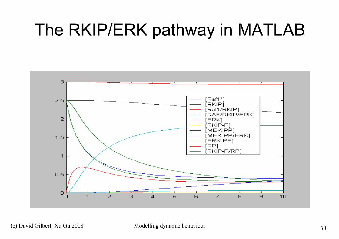
Description in MATLAB:3. The RKIP/ERK pathway
function dydt = erk_pathway_wolkenhauer(t, y)% from Kwang-Hyun Cho et al., Mathematical Modeling...k1 = 0.53;k2 = 0.0072;k3 = 0.625;k4 = 0.00245;k5 = 0.0315;k6 = 0.8;k7 = 0.0075;k8 = 0.071;k9 = 0.92;k10 = 0.00122;k11 = 0.87;

(c) David Gilbert, Xu Gu 2008 Modelling dynamic behaviour 37
Description in MATLAB:3. The RKIP/ERK pathway
Analysis of the model:>> [t y] =ode45(@erk_pathway_wolkenhauer, [010], [2.5 2.5 0 0 0 0 2.5 0 2.5 30]); %(initial values!)
>> plot (t, y);>> legend ('[Raf1*]', '[RKIP]','[Raf1/RKIP]', '[RAF/RKIP/ERK]','[ERK]', '[RKIP-P]', '[MEK-PP]','[MEK-PP/ERK]', '[ERK-PP]', '[RP]','[RKIP-P/RP]' );
(c) David Gilbert, Xu Gu 2008 Modelling dynamic behaviour 38
The RKIP/ERK pathway in MATLAB

(c) David Gilbert, Xu Gu 2008 Modelling dynamic behaviour 39
Further Analyses in MATLAB et al.
All initial concentrations can be varied at will, e.g. to test aconcentration series of one component (sensitivity analysis)
Effect of slightly different k-values can be tested (stability of the modelwith respect to measurement/estimation errors)
Effect of inhibitors of each reaction (changed k-values) can bepredicted
Concentrations at each time-point are predicted exactly and can betested experimentally

(c) David Gilbert, Xu Gu 2008 Modelling dynamic behaviour 40
Example of Sensitivity Analysisfunction [tt,yy] = sensitivity(f, range, initvec,
which_stuff_vary, ep, step, which_stuff_show, timeres);
timevec = range(1):timeres:range(2);vec = [initvec];[tt y] = ode45(f, timevec, vec);yy = y(:,which_stuff_show);
for i=initvec(which_stuff_vary)+step:step:ep; vec(which_stuff_vary) = i; [t y] = ode45(f, timevec, vec); tt = [t]; yy = [yy y(:,which_stuff_show)];end

(c) David Gilbert, Xu Gu 2008 Modelling dynamic behaviour 41
Example of Sensitivity Analysis
>> [t y] =sensitivity(@erk_pathway_wolkenhauer, [0 1], [2.5 2.5 0 0 0 0 2.5 02.5 3 0], 5, 6, 1, 8, 0.05);
>> surf (y);varies concentration of m5 (ERK-PP) from 0..6,
outputs concentration of m8 (ERK/MEK-PP), timerange [0 1], steps of 0.05. Then plots a surfacemap.

(c) David Gilbert, Xu Gu 2008 Modelling dynamic behaviour 42
Example of Sensitivity Analysis
after Cho et al. (2003) CSMB

(c) David Gilbert, Xu Gu 2008 Modelling dynamic behaviour 43
Example of Sensitivity Analysis(longer time course)

(c) David Gilbert, Xu Gu 2008 Modelling dynamic behaviour 44
Simulation in BioNessie

(c) David Gilbert, Xu Gu 2008 Modelling dynamic behaviour 45
SBML: http://www.sbml.org
• The Systems Biology Markup Language (SBML) is a computer-readable format for representing models of biochemicalreaction networks. SBML is applicable to metabolic networks, cell-signaling pathways, regulatory networks, and manyothers.
• SBML has been evolving since mid-2000 through the efforts of an international group of software developers and users.Today, SBML is supported by over 75 software systems including Gepasi. Also an SBML->MatLab converter
• Advances in biotechnology are leading to larger, more complex quantitative models. The systems biology communityneeds information standards if models are to be shared, evaluated and developed cooperatively. SBML's widespreadadoption offers many benefits, including:
– enabling the use of multiple tools without rewriting models for each tool– enabling models to be shared and published in a form other researchers can use even in a different software environment– ensuring the survival of models (and the intellectual effort put into them) beyond the lifetime of the software used to create them.

(c) David Gilbert, Xu Gu 2008 Modelling dynamic behaviour 46
SBML - XML Based Language
<sbml><model>
<listOfCompartments> <compartment/> </listOfCompartments><listOfSpecies> <specie/> < /listOfSpecies><listOfReactions>
<reaction> <listOfReactants>
<specieReference/></listOfReactants><listOfProducts>
<specieReference/> </listOfProducts><kineticLaw>
<listOfParameters> <parameter/> </listOfParameters>
</kineticLaw></reaction>
</listOfReactions></model></sbml>

(c) David Gilbert, Xu Gu 2008 Modelling dynamic behaviour 47
SBML Example
Specie representation: m1 in RKIP model:<specie name="m1" compartment="compartment" initialAmount="2.5" boundaryCondition="false" />
Reaction representation: k1 in RKIP model: m1 + m2 -> m3 (rate = k1 = 0.53)<reaction name="k1" reversible="false">
<listOfReactants> <specieReference specie="m1" stoichiometry="1" /><specieReference specie="m2" stoichiometry="1" /></listOfReactants>
<listOfProducts><specieReference specie="m3" stoichiometry="1" /></listOfProducts>
<kineticLaw formula="k_1*m1*m2"><listOfParameters><parameter name="k_1" value="0.53" /></listOfParameters></kineticLaw>
</reaction>

(c) David Gilbert, Xu Gu 2008 Modelling dynamic behaviour 48
How to model
Identification
Simulation
DefinitionAnalysis ValidationYes No
Slide fromRichard Orton
(c) David Gilbert, Xu Gu 2008 Modelling dynamic behaviour 49
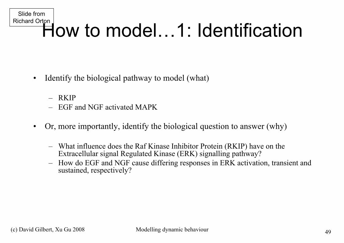
How to model…1: Identification
• Identify the biological pathway to model (what)
– RKIP– EGF and NGF activated MAPK
• Or, more importantly, identify the biological question to answer (why)
– What influence does the Raf Kinase Inhibitor Protein (RKIP) have on theExtracellular signal Regulated Kinase (ERK) signalling pathway?
– How do EGF and NGF cause differing responses in ERK activation, transient andsustained, respectively?
Slide fromRichard Orton

(c) David Gilbert, Xu Gu 2008 Modelling dynamic behaviour 50
How to model…2: Definition• This is the key step and is not trivial
• Draw a detailed picture of the pathway to model– Define all the proteins/molecules involved– Define the reactions they are involved in– Where do you draw the model boundary line?
• Check the literature– What is known about the pathway and proteins?– What evidence is there that protein A binds directly to protein B?– Protein C also binds directly to protein B: does it compete with protein A or
do they bind to protein B at different sites?– Trust & Conflicts: it is important to recognize which evidence to trust and
which to discard (talk to the people in the wet lab)
• Simplifying assumptions– Many biological processes are very complex and not fully understood– Therefore, developing a model often involves making simplifying
assumptions– For example, the activation of Raf by Ras is very complicated and not fully
understood but it is often modelled as:• Raf + Ras-GTP = Raf/Ras-GTP -> Raf-x + Ras-GTP
– Although this is a simplification, it is able to explain the observed data
Slide fromRichard Orton

(c) David Gilbert, Xu Gu 2008 Modelling dynamic behaviour 51
How to model…2: Definition• Define the kinetic types
– Each reaction has a specific kinetic type– All the reactions in the RKIP model are mass action (plain,
uncatalysed kinetic type):• V = k1[m1][m2 ] - k2[m3]
– Another common kinetic type is Michaelis Menten (enzymecatalysis):
• V = Vmax[S] / (Km+[S])
• Define the rate constants (k’s, km’s, Vmax’s etc)
• Define the initial concentrations
• Check the literature
– What values have been previously reported?– What values are used in similar models?– Do you trust them? Are there any conflicts?– Measure them yourself in the wet lab– Parameter estimation techniques: estimate some parameters based
on others and observed data
Slide fromRichard Orton

(c) David Gilbert, Xu Gu 2008 Modelling dynamic behaviour 52
How to model…3: Simulation
• Once the model has been constructed and parameter data hasbeen assigned you can simulate (run) the model
• This is a relatively straightforward step as there are manysoftware tools available to simulate differential equation basedmodels
• For example:
– BioNessie– MatLab– Copsai / Gepasi– CellDesigner– Jarnac– WinScamp– Many many more
• Runtime options include setting the time to run the model forand the number of data points to take
Slide fromRichard Orton

(c) David Gilbert, Xu Gu 2008 Modelling dynamic behaviour 53
How to model…4: Validation• Simulating the model typically returns a table of data which
shows how each specie’s concentration varies over time
• This table can then be used to generate graphs of specieconcentrations
• Do the model results match the experimental data?– Yes: validation– No: back to definition and check for errors
• Simple typos• Wrong kinetics• Over simplifications of processes• Missing components from the model• Incorrect parameter data
• The model can then be validated further by checking thesystem behaves correctly when things are varied:
– It might be known how the system behaves when you over-express or knockout a component
– The model should be able to recreate this behaviour
• If the model’s results do not match known biology, we cannotrely on predictions about unknown biology
Slide fromRichard Orton

(c) David Gilbert, Xu Gu 2008 Modelling dynamic behaviour 54
How to model…5: Analysis• After the model has been validated we can then analyse and interpret the results
– What do the results imply or suggest?– What do they tell us that is new and that we did not know/understand before?– What predictions can we make?
• Sensitivity analysis can be used to identify the key steps and components in the pathway as well asmonitoring how robust the system is:
– Vary an initial concentration or rate by a small amount and see what affect it has on the system as a whole:small changes in a key value are likely to have a large affect
– How robust is the system to changes?
• Knockout experiments are easy to do in a model: for example, simply set the initial concentration ofthe desired component to 0
– Knockout experiments can be used to identify which components are essential and which are redundant– Can also knockout reactions (set rate to 0) to identify essential and redundant reactions in the system
Slide fromRichard Orton

(c) David Gilbert, Xu Gu 2008 Modelling dynamic behaviour 55
How to model…Overview
Identification
Simulation
DefinitionAnalysis ValidationYes No
Slide fromRichard Orton
(c) David Gilbert, Xu Gu 2008 Modelling dynamic behaviour 56
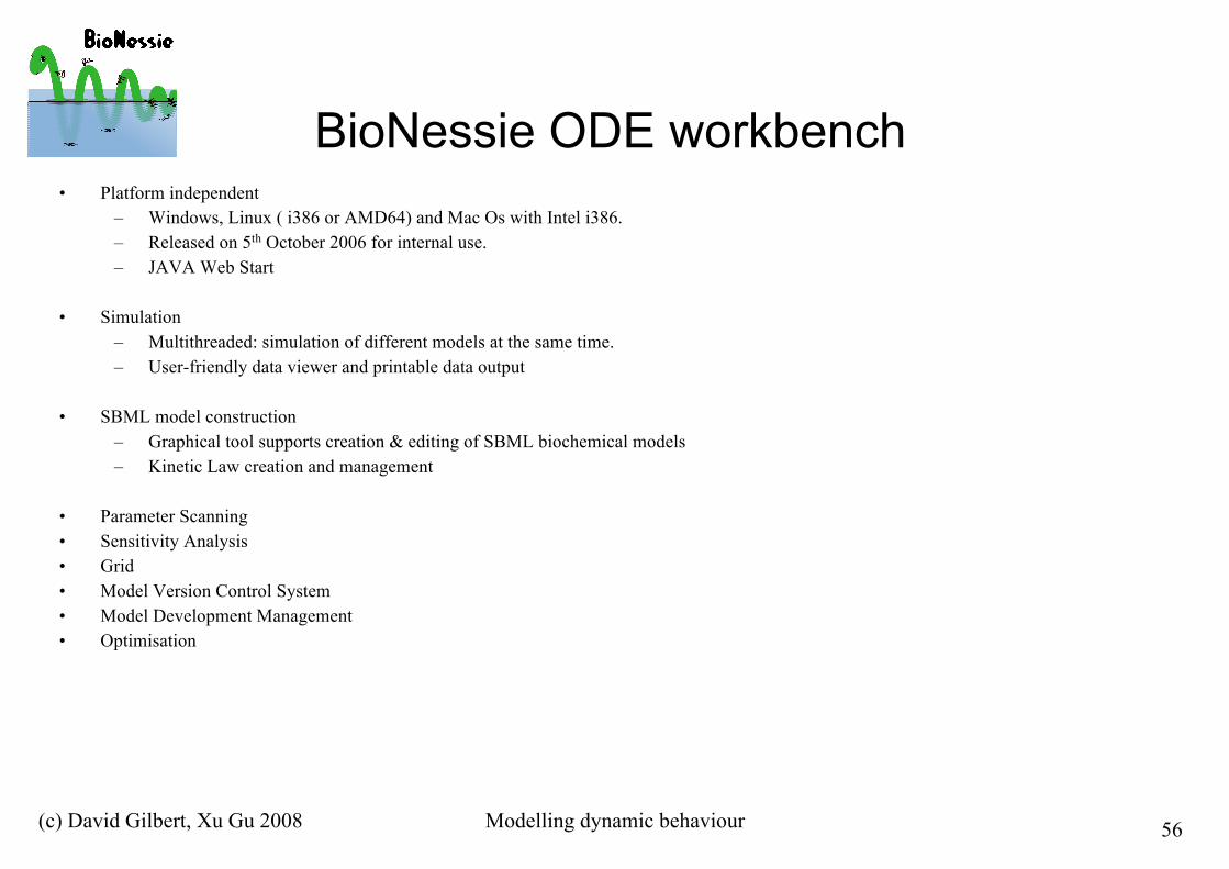
BioNessie ODE workbench• Platform independent
– Windows, Linux ( i386 or AMD64) and Mac Os with Intel i386.– Released on 5th October 2006 for internal use.– JAVA Web Start
• Simulation– Multithreaded: simulation of different models at the same time.– User-friendly data viewer and printable data output
• SBML model construction– Graphical tool supports creation & editing of SBML biochemical models– Kinetic Law creation and management
• Parameter Scanning• Sensitivity Analysis• Grid• Model Version Control System• Model Development Management• Optimisation


(c) David Gilbert, Xu Gu 2008 Modelling dynamic behaviour 58
Simulator, analyser...& go-faster on the Grid!
Xuan Liu, Vladislav Vyshemirsky,Gary Gray, Jipu Jiang, Femi Ajayi(David Gilbert, Richard Sinnott)
Grid Nodes
… … …
Sending JobReceiving Results
Results Collector Grid Web Service
Cluster

(c) David Gilbert, Xu Gu 2008 Modelling dynamic behaviour 59
Multi-threaded Parameter Scan
Slide from Xuan Liu

(c) David Gilbert, Xu Gu 2008 Modelling dynamic behaviour 60
This plot shows the whole trace of selected species - ERKPP for a parameter scan in RKIPpathway.xml of parameter K2 from 0 through 4.5 insteps of 0.5 with linear density for the timecourse of 100 timesteps of 100 time units.
Slide from Xuan Liu
(c) David Gilbert, Xu Gu 2008 Modelling dynamic behaviour 61
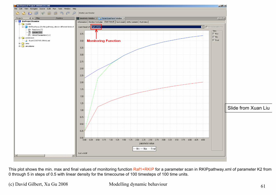
This plot shows the min. max and final values of monitoring function Raf1+RKIP for a parameter scan in RKIPpathway.xml of parameter K2 from0 through 5 in steps of 0.5 with linear density for the timecourse of 100 timesteps of 100 time units.
Slide from Xuan Liu

(c) David Gilbert, Xu Gu 2008 Modelling dynamic behaviour 62
• Sensitivity analysis investigates the changes in the system outputs or behavior with respect to theparameter variations. It is a general technique for establishing the contribution of individualparameter values to the overall performance of a complex system.
• Sensitivity analysis is an important tool in the studies of the dependence of a system on externalparameters, and sensitivity considerations often play an important role in the design of controlsystems.
• Parameter sensitivity analysis can also be utilised to validate a model’s response and iteratively,to design experiments that support the estimation of parameters
Sensitivity analysis
Slide from Xuan Liu

(c) David Gilbert, Xu Gu 2008 Modelling dynamic behaviour 63
Sensitivity Analysis Creation in BioNessie
Slide from Xuan Liu

(c) David Gilbert, Xu Gu 2008 Modelling dynamic behaviour 64
This creates a plot of the sensitivity of species Raf1, RKIP, Raf1RKIP, ERKPP, Raf1RKIPERKPP, ERK, RKIPP, MEKPP,MEKPPERK, RP and RKIPPRP to the values of the parameter K6 for the timecourse of 200 timesteps of 200 time units.
Slide from Xuan Liu

(c) David Gilbert, Xu Gu 2008 Modelling dynamic behaviour 65
Other simulators include…
Copasi
MatLab & SimBio

(c) David Gilbert, Xu Gu 2008 Modelling dynamic behaviour 66
more simulators …
SBW - standard parts

(c) David Gilbert, Xu Gu 2008 Modelling dynamic behaviour 67
Human African Trypanosomiasis
• Numbers hit around 300,000 atthe end of the twentieth century
• Drugs exist, but not satisfactorye.g the arsenical melarsoprol
(c) David Gilbert, Xu Gu 2008 Modelling dynamic behaviour 68
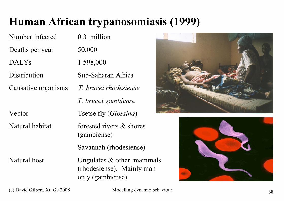
Human African trypanosomiasis (1999)Number infected 0.3 million
Deaths per year 50,000
DALYs 1 598,000
Distribution Sub-Saharan Africa
Causative organisms T. brucei rhodesiense
T. brucei gambiense
Vector Tsetse fly (Glossina)
Natural habitat forested rivers & shores (gambiense)
Savannah (rhodesiense)
Natural host Ungulates & other mammals (rhodesiense). Mainly man only (gambiense)
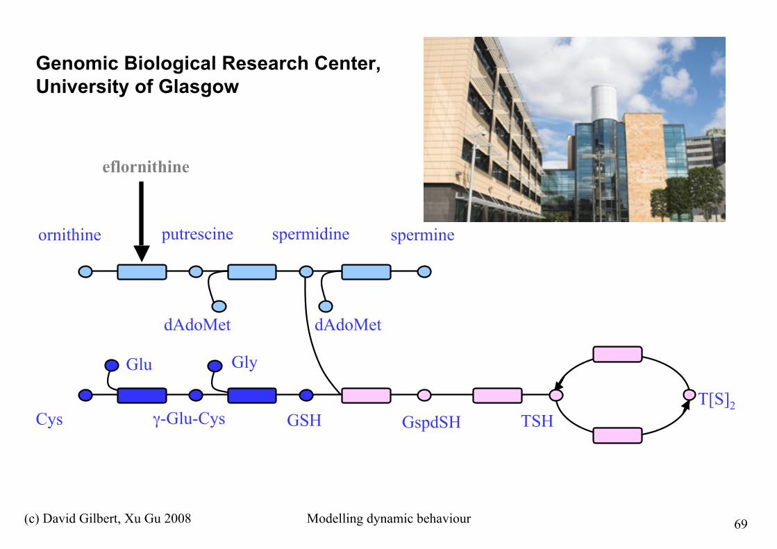
(c) David Gilbert, Xu Gu 2008 Modelling dynamic behaviour 69
T[S]2
ornithine putrescine spermidine spermine
Cys
Glu
γ-Glu-Cys GSH GspdSH TSH
Gly
dAdoMet dAdoMet
eflornithine
Genomic Biological Research Center,University of Glasgow

(c) David Gilbert, Xu Gu 2008 Modelling dynamic behaviour 70
Trypanothionine ODE model

(c) David Gilbert, Xu Gu 2008 Modelling dynamic behaviour 71
Kinetic Data
A black art?

(c) David Gilbert, Xu Gu 2008 Modelling dynamic behaviour 72
Conclusions and Outlook
• Differential equations allow exact predictions of systems behaviourin a unified formalism
• Modelling = in silico experimentation• Difficulties:
– translation from biology• modular model building interfaces, e.g. Gepasi/COPASI, Genomic Object Net, E-
cell, Ingeneue– managing complexity explosion
• pathway visualization and construction software• standardized description language, e.g. Systems Biology Markup Language
(SBML)– lack of biological data
• perturbation-based parameter estimation, e.g. metabolic control analysis (MCA)• constraints-based modelling, e.g. flux balance analysis (FBA)• semi-quantitative differential equations for inexact knowledge
© Rainer Breitling

Modelling and modularisation
Example:Signalling pathway cascades

(c) David Gilbert, Xu Gu 2008 Modelling dynamic behaviour 74
Mass action for enzymatic reaction -phosphorylation
• R: substrate,• Rp: product (phosphorylated R)• S1: enzyme (kinase)• R|S1 substrate-enzyme complex
!
R+S1
k2" # #
k1# $ # R | S
1
k3# $ # Rp + S
1
R Rp
S1

(c) David Gilbert, Xu Gu 2008 Modelling dynamic behaviour 75
Phosphorylation - dephosphorylation loopMass action model 1
• R: unphosphorylated form• Rp: phosphorylated form• S1: kinase• S2: phosphotase• R|S1 unphosphorylated+kinase complex• R|S2 unphosphorylated+phosphotase complex
R Rp
S1
S2
!
R+S1
k2" # #
k1# $ # R | S
1
k3# $ # Rp + S
1
R+S2
k3'
" # # Rp | S2k2 '
# $ #
k1 '" # # Rp + S
2

(c) David Gilbert, Xu Gu 2008 Modelling dynamic behaviour 76
Phosphorylation cascade:2-stage, Mass Action model 1
RpR
S1
RRpRR
!
R+S1
k2" # #
k1# $ # R | S
1
k3# $ # Rp + S
1
R+S2
k3'
" # # R | S2
k2 '# $ #
k1 '" # # Rp + S
2
RR + Rpkk2
" # #
kk1# $ # RR |Rp
kk3# $ # RRp + Rp
RR+ SS2
kk3'
" # # RR | SS2
kk2 '# $ # #
kk1 '" # # # RRp + SS
2
S2
SS2

(c) David Gilbert, Xu Gu 2008 Modelling dynamic behaviour 77
Phosphorylation cascade:3-stage, Mass-Action model 1
RpR
S1
RRpRR
RRRpRRR
!
R+S1
k2" # #
k1# $ # R | S
1
k3# $ # Rp + S
1
R+S2
k3'
" # # Rp | S2k2 '
# $ #
k1 '" # # Rp + S
2
RR + Rpkk2
" # #
kk1# $ # RR |Rp
kk3# $ # RRp + Rp
RR+ SS2
kk3'
" # # RRp | SS2kk2 '
# $ # #
kk1 '" # # # RRp + SS
2
RRR + RRpkkk2
" # # #
kkk1# $ # # RRR |RRp
kkk3# $ # RRRp + RRp
RRR+ SSS2
kkk3'
" # # # RRRp | SSS2kkk2 '
# $ # #
kkk1 '" # # # RRRp + SSS
2
S2
SS2
SSS2

(c) David Gilbert, Xu Gu 2008 Modelling dynamic behaviour 78
Phosphorylation cascade + negative feedback: 3-stage, Mass Action, model 1
RpR
S1
RRpRR
RRRpRRR
!
RRRp+S1ki '
" # #
ki# $ # RRRp | S1
R+S1
k2" # #
k1# $ # R | S
1
k3# $ # Rp + S
1
R+S2
k3'
" # # Rp | S2k2 '
# $ #
k1 '" # # Rp + S
2
RR + Rpkk2
" # #
kk1# $ # RR |Rp
kk3# $ # RRp + Rp
RR+ SS2
kk3'
" # # RRp | SS2kk2 '
# $ # #
kk1 '" # # # RRp + SS
2
RRR + RRp1kkk2
" # # #
kkk1# $ # # RRR |RRp
kkk3# $ # RRRp + RRp
RRR+ SSS2
kkk3'
" # # # RRRp | SSS2kkk2 '
# $ # #
kkk1 '" # # # RRRp + SSS
2
S2
SS2
SSS2

(c) David Gilbert, Xu Gu 2008 Modelling dynamic behaviour 79
Phosphorylation cascade + negative feedback: 3-stage, Inhibitor on 2nd stage, Mass Action
!
RRRp+S1ki '
" # #
ki# $ # RRRp | S1
R+S1
k2" # #
k1# $ # R | S
1
k3# $ # Rp + S
1
R+S2
k3'
" # # Rp | S2k2 '
# $ #
k1 '" # # Rp + S
2
RR + Rpkk2
" # #
kk1# $ # RR |Rp
kk3# $ # RRp + Rp
RR+ SS2
kk3'
" # # RRp | SS2kk2 '
# $ # #
kk1 '" # # # RRp + SS
2
U + RRku2
" # #
ku1# $ # # U |RR
U + RR pku2
" # #
ku1# $ # # U |RR p
U |RR + Rpkk2
" # #
kk1# $ # U |RR |Rp
kk3# $ # U |RRp + Rp
U |RR+ SS2
kk3'
" # # U |RR p| SS2kk2 '
# $ # #
kk1 '" # # # U |RRp + SS
2
RRR + RRpkkk2
" # # #
kkk1# $ # # RRR |RRp
kkk3# $ # RRRp + RRp
RRR+ SSS2
kkk3'
" # # # RRRp | SSS2kkk2 '
# $ # #
kkk1 '" # # # RRRp + SSS
2
RpR
S1
RRpRR
RRRpRRR
U|RRpU|RR
S2
SSS2

(c) David Gilbert, Xu Gu 2008 Modelling dynamic behaviour 80
Further Analyses
All initial concentrations can be varied at will, e.g. to test aconcentration series of one component (sensitivity analysis)
Effect of slightly different k-values can be tested (stability of the modelwith respect to measurement/estimation errors)
Effect of inhibitors of each reaction (changed k-values) can bepredicted
Concentrations at each time-point are predicted exactly and can betested experimentally
© Rainer Breitling
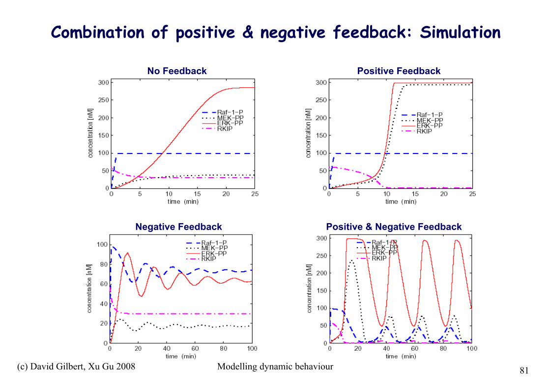
(c) David Gilbert, Xu Gu 2008 Modelling dynamic behaviour 81
No Feedback Positive Feedback
Negative Feedback Positive & Negative Feedback
Combination of positive & negative feedback: Simulation

(c) David Gilbert, Xu Gu 2008 Modelling dynamic behaviour 82
Combination of positive & negative feedback:Simulation vs. Experimental Data
0 20’ 40’ 1h 2h 3h 4h 6h TPA
ERK-pp (activated ERK)
total ERK
Western blots COS1 cell lysates
0 1 2 3 4 5 60
0.1
0.2
0.3
0.4
0.5
0.6
0.7
0.8
0.9
1
Time [hour]
Normal.[unitless]
Comparison of experimentad data and simulation result
m5(erk-pp)
raw-erk
Simulation
Experiment

(c) David Gilbert, Xu Gu 2008 Modelling dynamic behaviour 83
Lecture outline• Biochemical reactions• Modelling with Ordinary Differential Equations• Kinetics : Mass Action• Examples
– Signalling & metabolic pathways– Trypanothione metabolism in Trypanosoma brucei– Oscillators & Amplifiers
• Analysis• ODE simulators


