Instructions for use

Title Biological effect of dose distortion by fiducial markers in spot-scanning proton therapy with a limited number of fields:A simulation study

Author(s)Matsuura, Taeko; Maeda, Kenichiro; Sutherland, Kenneth; Takayanagi, Taisuke; Shimizu, Shinichi; Takao, Seishin;Miyamoto, Naoki; Nihongi, Hideaki; Toramatsu, Chie; Nagamine, Yoshihiko; Fujimoto, Rintaro; Suzuki, Ryusuke;Ishikawa, Masayori; Umegaki, Kikuo; Shirato, Hiroki

Citation Medical Physics, 39(9), 5584-5591https://doi.org/10.1118/1.4745558

Issue Date 2012-09

Doc URL http://hdl.handle.net/2115/50429

Type article (author version)

File Information MP39-9_5584-5591.pdf

Hokkaido University Collection of Scholarly and Academic Papers : HUSCAP

1

November 13, 2012

Biological effect of dose distortion by fiducial markers in spot-scanning proton therapy with a

limited number of fields: a simulation study

Running head: Biological effect of proton dose-distortion by fiducials

Taeko Matsuura1, Kenichiro Maeda

1, Kenneth Sutherland

1, Taisuke Takayanagi

2, Shinichi Shimizu

2,

Seishin Takao1, Naoki Miyamoto

1, Hideaki Nihongi

1, Chie Toramatsu

1, Yoshihiko Nagamine

4,

Rintaro Fujimoto3, Ryusuke Suzuki

1, Masayori Ishikawa

1, Kikuo Umegaki

2, Hiroki Shirato

2

1Department of Medical Physics, Hokkaido University Graduate School of Medicine

2Hitachi, Ltd., Hitachi Research Laboratory

3Department of Radiation Medicine, Hokkaido University Graduate School of Medicine

4Hitachi, Ltd., Hitachi Works

Address correspondence to: Taeko Matsuura PhD

Graduate School of Medicine, Hokkaido University, North 15, West 7, Kita-ku, Sapporo, Hokkaido, 060-8638,

Japan

Tel.: +81- 11 - 706- 5254, Fax: +81- 11 -706 -5254

E-mail: matsuura@med.hokudai.ac.jp

2

ABSTRACT

Purpose: In accurate proton spot-scanning therapy, continuous target tracking by fluoroscopic X-ray during

irradiation is beneficial not only for respiratory moving tumors of lung and liver but also for relatively stationary

tumors of prostate. Implanted gold markers have been used with great effect for positioning the target volume by a

fluoroscopy, especially for the cases of liver and prostate with the targets surrounded by water-equivalent tissues.

However, recent studies have revealed that gold markers can cause a significant underdose in proton therapy. This

paper focuses on prostate cancer and explores the possibility that multiple-field irradiation improves the underdose

effect by markers on Tumor Control Probability (TCP).

Methods: A Monte Carlo simulation was performed to evaluate the dose distortion effect. A spherical gold

marker was placed at several characteristic points in a water phantom. Markers were with two different diameters

of 2 mm and 1.5 mm, both visible on fluoroscopy. Three beam arrangements of SFUD (single-field uniform dose)

were examined: one lateral field, two opposite lateral fields, and three fields (two opposite lateral fields + anterior

field). The Relative Biological Effectiveness (RBE) was set to 1.1 and a dose of 74 Gy (RBE) was delivered to the

target of a typical prostate size in 37 fractions. The ratios of TCP to that without the marker (TCPr) were compared

with the parameters of the marker sizes, number of fields, and marker positions. To take into account the

dependence of biological parameters in TCP model, values of 1.5, 3, and 10 Gy (RBE) were considered.

Results: It was found that the marker of 1.5 mm diameter does not affect the TCPs with all values when two

or more fields are used. On the other hand, if the marker size is 2 mm, more than two irradiation fields are

required to suppress the decrease in TCP from TCPr by less than 3%. This is especially true when multiple (two or

three) markers are used for alignment of a patient.

Conclusions: It is recommended that 1.5 mm markers be used to avoid the reduction of TCP as well as to spare

the surrounding critical organs, as long as the markers are visible on X-ray fluoroscopy. When 2 mm markers are

implanted, more than two fields should be used and the markers should not be placed close to the distal edge of

any of the beams.

Key Words: Proton spot-scanning therapy, Tumor tracking, Fiducial marker, Prostate cancer, Tumor Control

Probability

3

I. INTRODUCTION

The number of proton therapy centers which adopt the spot-scanning technique has been increasing worldwide.

Spot-scanning proton therapy has an advantage to achieve high dose conformity by changing the dosage and the

position of each pencil beam (spot) individually under computer control. However, at the same time, targeting

accuracy within the order of millimeters must be achieved by various image-guided radiotherapy (IGRT)

techniques. During irradiation, continuous target tracking by a fluoroscopic X-ray system is useful for respiratory

moving tumors1. It has been reported that even the prostate can undergo more than 10 mm of intra-fractional

motion during 1 minute2, which suggests that real-time tracking is also beneficial for the prostate

3. Due to their

high opacity, gold markers have been used with great effect especially for the cases of liver and prostate with the

targets surrounded by water-equivalent tissues. Gold fiducial markers have been in clinical use in proton therapy

centers4. However, recent studies have revealed that a certain size of cylindrical gold markers can cause as much

as 85% of proton underdose mainly due to their high electron density5,6,7

. Several proposals to mitigate dose

distortion have been made such as the reduction of marker size7, the optimization of marker compounds with

carbon-coated ceramic8 or mixture of microscopic gold particles and polymers

9.

An alternate solution may be to diminish the dose distortion effect by increasing the number of fields10

. Because

proton pencil beam scanning technique does not require replacement of the apertures and range compensators

field by field, the treatment time will not be increased so much by the use of multiple fields. On the other hand,

there is a limit to the number of fields. First of all, the low-dose region is expanded by an increase in the number

of fields, which could cancel the advantages of proton therapy. Secondly, for spot-scanning proton therapy, the

plan quality tends to be worse as the number of field exceeds a certain threshold when single-field optimization

(SFO) is used11

. This is due to the minimum monitor unit (MU) for delivering each spot, which is 0.005 MU at

our institution. Therefore, it is necessary to use a minimum number of fields while at the same time to control the

effect of dose distortion due to the presence of gold markers to be within an acceptable range.

In this research, we focus on prostate cancer and explore the possibility that multiple-field irradiation improves

the underdose effect by markers on Tumor Control Probability (TCP) using a Monte Carlo simulation. Three

beam arrangements of SFUD (single-field uniform dose) were examined: one lateral field, two opposite lateral

fields, and three fields (two opposite lateral fields + anterior field). More than three fields were not considered

4

because the MU constraint limits the number of fields to three for 2 Gy (RBE) irradiation to the target of a typical

prostate size with 8 mm spot spacing. We also investigated two different sizes of gold marker (2 mm and 1.5 mm

in diameter), which are both visible on fluoroscopy. They were placed at several positions in the prostate that have

different characteristics in terms of proton momentum distribution, which produce different dose distortions. We

considered multiple values of 1.5, 3, and 10 Gy (RBE)12,13,14

for the evaluation of TCP, because there are still

debate on value for prostate tumors at this moment. The required number of fields was then determined for

each marker size such that the TCP reduction is within an acceptable range for all position of a marker and for any

values.

II. MATERIALS AND METHODS

A. Simulation setup

Figure 1 shows the water phantom geometry, coordinate system, and beam directions. The phantom size (38×

20×20 cm3) was determined based on the average anatomical measurements of water equivalent length made

from computed tomography scans of 10 prostate cancer patients’ pelvises. Clinical target volume (CTV) was

defined as prostate and its size ranges from 28 to 74 cm3 (44 cm

3 on average) over the 10 patients. In the

simulation, it was represented as a cube of an equivalent volume placed at the center of the phantom and the side

length was 3-4.2 cm (3.5 cm on average). PTV margin of 3 mm, which is clinically used in Hokkaido University

Hospital for prostate IMRT, was added for each size of CTV.

The coordinate system is defined with respect to the treatment room; the origin is at the isocenter (IC) which

coincides with the center of the target. We considered the following three beam directions: right–lateral (gantry

angle 270 degrees, field 1), left–lateral (gantry angle 90 degrees, field 2), and anterior (gantry angle 0 degrees,

field 3). The proton absorbed-dose distributions were simulated using the Geant4 Monte Carlo code (ver. 4.9.4).

The binary cascade model15

was used for the nuclear interactions. The production thresholds for gamma, electrons

and positrons are needed to avoid the infrared divergences and they were all set to 0.1 mm. The Hokkaido

University spot-scanning beam treatment nozzle as well as the beam characteristics designed by Hitachi (Hitachi

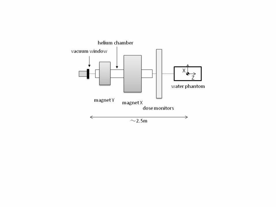
Ltd., Japan) was implemented (Figure 2). The spot size depends on the beam energy and it was 3.6 ~ 6.9 mm ()

at the IC in air. The primary protons were generated just above the vacuum window, which was located about 2.5

m from the IC. For one spot, we simulated 600,000 primary protons. The dose was scored in cubic volumes of 0.5

5

mm side length in order to obtain statistical uncertainty less than 2% at the distal border of the PTV.

Spot weight optimization was performed by SFUD. For all fields, the spacing between spots was set to 8 mm.

The simulation was made for minimum, average, and maximum size of CTV which are denoted as CTVmin,

CTVave, and CTVmax, respectively. For CTVave, iso-energy layers of 157-180 MeV (11 layers) were used for the

lateral beams (fields 1 and 2) and 103-132 MeV (21 layers) for the anterior beam (field 3). Fields 1 and 2 required

891 spots to cover the PTV volume, while field 3 needed 1701 spots. We assumed a dose prescription of 74 Gy

(RBE) in 37 fractions to the isocenter in accordance with a previous report16

. The Relative Biological

Effectiveness (RBE) was set to 1.1. When three fields were used, the minimum MU per spot was 0.007 for fields

1 and 2 and 0.005 for field 3 at the lowest iso-energy layer. This indicates that as long as we constrain ourselves to

SFUD with 8 mm spot spacing, the maximum field number is three for 2 Gy (RBE) irradiation to this target. The

calculated dose deviation from the prescribed dose comes from both small ripples within the spread-out Bragg

peaks in a treatment plan and statistical uncertainty. It was within ±5% for more than 99.9% of the CTV. In a

same manner, the dose distribution for CTVmin and CTVmax were constructed by using corresponding iso-energy

layers.

B. Gold marker placement

Two sizes of spherical gold marker with diameters of 2 mm and 1.5 mm were investigated. As shown in Figure 3,

both sizes were recognized by a fluoroscopy when inserted in a pelvic phantom (100 kV, 80 mAs, 4 msec (AP),

120 kV, 80 mAs, 4 msec (LR)). The fluoroscopic images of the 2 mm marker were clear, while those of the 1.5

mm marker might be not so clear to discern in some patients.

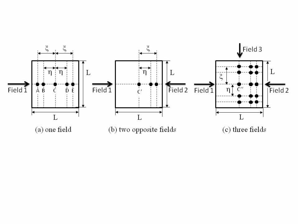
Markers were placed at several characteristic points for each beam arrangement (Fig. 4). In the case of one field,

5 points were considered: the IC (C), the proximal (A) and distal (E) points, and the intermediate points between

IC and the proximal point (B) and between IC and the distal point (D). In the case of two and three fields, the

representative 3 and 15 points were investigated, respectively. When a marker is placed at an off-central axis

position, the dose distortion due to the presence of the marker is assumed to be the parallel shift of that produced

when the marker is place at the central axis. This is a good approximation because the SOBP width is a constant

for the cubic PTV and because the marker positions are chosen so that they are more than 5 mm distant from the

PTV boundary. The dose distortion that occurs in a cylindrical region of a diameter less than 5 mm, does not

6

overlap with the PTV boundary (see Sec. III).

C. TCP model

In order to evaluate the biological effect of the dose distortion, TCP values were evaluated from the dose

distribution derived by the above-mentioned procedure. First of all, the linear quadratic (LQ) model was used for

the calculation of surviving fraction (SF):

E( )SF e ,D (1)

where

2E( ) .D D Dn

(2)

Here and characterize intrinsic radio-sensitivity, D is the total dose that is generally different from point to

point in the prostate, n is the number of dose fractions. Then, the Poisson TCP model:

SF( ( ))

TCP , in D i ci

voxel i voxel

Ve n

N

(3)

was used to link cell killing to bulk clinical effect where Nvoxel varies according to the CTV size (from 603 to 84

3 in

this simulation). D(i) is the local dose at the i-th voxel, c is the initial number density of clonogenic cells, V is the

CTV volume, and ni is the cell number in i-th voxel. We assume a uniform CTV clonogenic cell density of c =106

cm-3 17

. In the evaluation, the voxels that contain gold markers are excluded.

The biological parameters used in this study are summarized in Table 1. For each parameter set, the TCP curve

for homogeneous dose distribution was shown in Figure 5. Three values of 1.5, 3, and 10 Gy (RBE) were

examined. For a fixed , parameter was determined so that the TCP at 74 Gy (RBE) in 37 fractions is 94%

for CTVave. This value corresponds to the clinical data available on proton therapy. In report16

, it was shown that

biochemical relapse-free survival rate (bNED) at 3 years was 94% for Gleason score < 8 patient group. The

similar percentage is also seen in report18

in which bNED at 5-years was more than 92% for T1-T2a patients with

the same dose prescription. As far as the authors know, additional clinical data with different dose prescriptions

and same patient group was not available. With those data, the variability in clonogen sensitivities within a tumor

(ind) and/or the variability from patient to patient (pop) would be determined by curve fitting19,20

. In this study,

ind and pop are set to zero, which may result in an overestimation of TCP reduction by the underdosage20

.

7

D. Method of evaluation

The ratios of TCP to that without the marker (TCPr) were compared with the parameters of the marker sizes,

number of fields, and marker positions for each . For each parameter set, the ratio RTCP = TCP/TCPr was

obtained for three CTV volumes and the minimum value of those, namely RV

TCP = min{RTCP(CTVmin),

RTCP(CTVave), RTCP(CTVmax)}, were calculated. Here, as can be seen from eq. (3), TCPr decreases as the CTV

volume increases and it was 96%, 94%, and 90% for CTVmin, CTVave, and CTVmax, respectively. The tolerance for

TCP reduction is defined as TCP < 3%, where TCP ≡ 100×(1 - RV

TCP) (%). TCP for multiple markers is

approximately the sum of TCP’s caused by each marker as long as (1 - RV

TCP)≪1 is satisfied. In order to

understand the results, the depth dose distributions, the plane dose distribution along the central beam axis, and the

minimum dose in CTV (Dmin) were shown for CTVave.

III. RESULTS

A. Dose distribution

Figure 6 shows the depth dose distribution along the central beam axis for one field with both sizes of gold

markers. In each figure, three plots for one lateral field with marker positions (A), (C), and (E) in Figure 4 (a) are

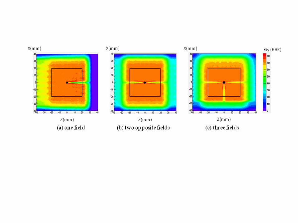
shown with the reference (without a marker). Figure 7 shows the plane dose distribution for one field (a), two

opposite fields (b), and three fields (c) along the central beam axis for gold markers with 2 mm placed at the IC,

which are (C), (C’), and (C’’) in Figure 4, respectively. Both graphs are shown for CTVave . The minimum dose is

listed in Table 2 for all conditions.

As shown in Fig. 6 and 7, the gold marker trails a thin cold line in the downstream region. Proton fluence is

reduced because protons stop in the gold marker or are strongly scattered by gold nuclei, i.e., Au ~ 6 .

Compared with the size of the CTV, however, the cold line thickness and its volume are sufficiently small, that is,

within the cylindrical region of 5 mm. The cold line length is shorter as the marker approaches the distal edge,

but at the same time, Dmin is further reduced because larger number of protons stops in the marker as well as the

fewer protons are scattered in the path by multiple Coulomb scattering (MCS). The exception is the case when the

marker is very close to the CTV boundary (a few mm). In that case, the point where the dose shadowing is

maximum is outside of CTV and it does not coincide with Dmin. For one field, Dmin is 24.1 Gy (RBE) (2 mm) and

8

39.4 Gy (RBE) (1.5 mm) when the marker is placed rather close to the distal edge ((D) or (E) in Figure 4). This

improves to Dmin = 51.4 Gy (RBE) (2 mm) and 57.9 Gy (RBE) (1.5 mm) by using three fields (see Table 2).

The minimum dose occurs at a position that is close to the distal edge for either one of the beams.

When a marker is placed upstream of the CTV, the recovery of the dose occurs downstream of the CTV (Fig. 6

(A) and (C)) because the neighboring protons scatter in the cold line. For 1.5 mm marker at position (A), the

dose recovers to almost 90 % of the reference at the downstream boundary of the CTV.

When the protons have such high energy at the marker position that they do not stop in the marker, they are

strongly scattered and create a hot shell surrounding the cold line (see Fig. 7). The maximum dose is then 86 Gy

(RBE) (2 mm) and 84 Gy (RBE) (1.5 mm) for one field and is reduced to 81 Gy (RBE) (2 mm) and 80 Gy

(RBE) (1.5 mm) for two opposite fields.

B. TCP comparison

In Table 2, values of RV

TCP are listed for all conditions. First of all, RV

TCP is smallest when of 1.5 Gy (RBE)

is used because the TCP curve is steeper for smaller and the underdosage more severely affects the TCP

reduction (Figure 5). With of 1.5 Gy (RBE), even when 1.5 mm marker is used, TCP can be as large as

36% if only one field is used. Generally the TCP gets worse as the marker is placed downstream of the CTV

because Dmin also decreases. RV

TCP even reaches zero when 2 mm marker is placed at position (D) and (E). When

the marker position is shifted from (D) to (E), the increase of RV

TCP can be seen for all . This is because the

overlap of dose shaded volume and CTV decreases and/or the minimum dose Dmin itself increases as the marker

shifts to downstream.

The TCP is greatly improved by using two opposing fields. TCP is less than 3% for 2 mm and less than 0.5%

for 1.5 mm marker for any position even when of 1.5 Gy (RBE) was used. If three fields are used, TCP is

less than 1% for any position when the 2 mm marker is used while it is less than 0.5% when the 1.5 mm marker

is used.

IV. DISCUSSION

In this research, we have studied the effect of dose distortion in the presence of implanted gold markers on TCP

in prostate cancer. A marker of 1.5 mm diameter does not affect the TCPs with any of 1.5, 3, and 10 Gy

9

(RBE) when two or more fields are used. On the other hand, if a marker of 2.0 mm diameter is used, it is safe to

use more than two fields especially when multiple markers (two or three) are used in order to suppress the sum of

TCP’s caused by each marker by less than 3%. It is recommended that 1.5 mm markers be used to avoid the

reduction of TCP as well as to spare the surrounding critical organs as long as they are visible on fluoroscopy. In

addition, it is preferable to place the markers so that they are not close to the distal edge for any of the beams. It is

worth mentioning that when multiple markers are used, they have to be placed so that the dose-distorted regions

do not overlap with each other. This is achieved by slightly shifting the gantry and/or couch rotation angle by

referring to the CT images.

It is clear that the Dmin approaches the reference value (without a marker) by the use of multiple-field irradiation,

but it is not a priori obvious whether the increase of fields improves the TCP. Indeed, multiple-field irradiation

can mitigate the local dose distortion, but at the same time, the dose shaded region may be expanded. Our results

indicate that, as long as 2 mm or 1.5 mm markers are used, such dose shaded regions are sufficiently small

(0.6% of CTV volume at maximum). The improvement of dose distortion by increasing the number of fields

surpasses the expanding of the dose shaded region, resulting in an improvement of TCP. The number of fields is

however limited by the minimum deliverable amounts for each spot, spacing between spots, and beam size. In our

nozzle, if spot spacing is set at 8 mm, which is about 1.6 times the smallest spot size at the Bragg-peak, three fields

is the upper limit for SFUD. It is possible that the number of fields can be increased by the use of Intensity

Modulation Proton Therapy (IMPT) plans. By IMPT, however, the proton momentum distribution at certain

points is highly dependent on the optimization algorithm as well as the CT images of each patient. It is then

difficult to figure out the possible size of the dose distortion and resulting TCPs. SFUD may be safer and simpler

from this point of view.

In this research, we performed spot weight optimization on a phantom with fiducial markers removed artificially.

The dose distribution is then calculated by returning them to the original positions. This procedure for

optimization should also be applied in clinical practice because if spot weight optimization is performed in the

presence of markers, there might be a large dose error when the patient geometry changes in an occasion when the

prostate deforms or the relative position between the prostate and bones changes. In the dose calculation, it may be

difficult or even not worthwhile in reality to restore the markers to the CT image. This is because the manual

assignment of gold markers in CT images21

is demanding since the slice thickness and pixel width of the CT

10

images are comparable to the marker size. Also, metal artifact9 prevents pinpointing the marker position. Even if

the assignment were possible, a high-precision dose calculation algorithm such as Monte Carlo simulation is

required to reproduce the dose disturbance, which is time-consuming. Therefore, it may be a reasonable strategy

to perform the dose calculation using the CT image with the marker removed, while implementing the

methodology so that the unseen dose distortion does not result in significant effects.

The metal artifacts caused by gold markers may be reduced using proposed metal artifact reduction algorithms

for helical CT22

or using the image registration technique between helical CT image and cone beam CT image

with metal artifact removed23

. The proton range precision with these metal-artifact-free CTs should be

investigated in future.

Gold markers are also used for accurate patient alignment and motion management for other sites such as liver

and lung. In such cases, the marker is generally placed outside of tumor, which may mitigate the possibility of

severe dose distortion since our results indicate that the more proximal region the marker is placed, the less dose

distortion it occurs. Detailed study on this issue will be carried out in the future.

The shape of the gold marker is limited to a sphere in this study. With the spherical symmetry, it has the

advantage over other shape of marker in that the precise 3-dimensional real-time tracking is possible even if the

markers rotate during the treatment. On the other hand, the commercially available helical gold markers have an

advantage that it may be more stable against migration. According to the Monte Carlo simulation7, however, it

causes more severe dose shadowing than the marker considered in this study. The smallest implantable marker

(0.75 mm in diameter and 1 cm in length) can cause as much as 64.1% of underdose when two opposite field is

used and the markers are parallel to the beam. This may be because the length of the marker is so long that it

greatly reduces the proton fluence in downstream. With this size of underdose, the non-negligible size of TCP

reduction is inevitable.

In this study, we neglected the effect of inter- and intra- fractionated tumor motions on TCP. Indeed, by using the

real-time tracking of gold markers, both inter- and intra- fractional prostate motions can be suppressed within 2

mm3. Therefore, we consider it a good approximation to neglect these motions in this study. Moreover, in ref

24, it

was shown that the effect of inter- and intra- fractional motion on TCP is small (< 2 %) with patient set up using

internal markers.

Finally, our study has several limitations. Firstly, the PTV margin that we considered may not be sufficiently

11

large to include the proton range uncertainty. However, the dose distortion and TCP values are expected to be

improved with the enlargement of the margin since there is a greater possibility that the marker is placed farther

from the distal edge. Secondly, the calculated dose perturbation has not been confirmed by measurement. Thirdly,

the dose distortion in a water phantom as well as cubic shape of the CTV may simplify the heterogeneous patient

anatomy. Finally, fiducial markers composed of other materials that may also be visible on fluoroscopy have not

been explored. Additional study of these issues should be undertaken in the future.

IV. CONCLUSIONS

In this research, we explored the possibility that multiple-field irradiation improves the underdose effect by

implanted gold markers on TCP in prostate cancer for spot-scanning proton therapy. Two sizes of spherical gold

marker with diameters of 2 mm and 1.5 mm were recognized by fluoroscopy when inserted in a pelvic phantom.

For both markers, dose distortion is generally more severe when the marker is close to the distal edge of CTV. A

gold marker with 1.5 mm diameter does not affect the TCPs derived from different biological parameters ()

and at any position in CTV when two or more fields are used. On the other hand, if multiple gold markers of 2.0

mm diameter are used, it is safe to use more than two fields and place the markers at a distance from the distal

edge for all the beams in order to suppress the decrease in TCP from TCPr by less than 3%.

Acknowledgements

This research is supported by the Japan Society for the Promotion of Science (JSPS) through the “Funding

Program for World-Leading Innovative R&D on Science and Technology (FIRST Program),” initiated by the

Council for Science and Technology Policy (CSTP). This work was partly supported by Grant-in-Aid for Young

Scientists (B) 23791379.

APPENDIX A: VALIDATION OF MONTE CARLO CODE

The proton range and size of multiple Coulomb scattering in water and gold were validated with NIST database 25

and analytical approximation formula of Highland26

, respectively.

(1) Proton Range

We considered the relevant four energies of E=103, 132, 157, and 180 MeV. They are the minimum and

12

maximum energies for lateral and anterior beams, respectively. The range in the present MC system was obtained

by simulating 105 protons with all physics processes switched off except for ionization

26,27. In that case, the depth

z80 at which the dose has dropped to 80% of its maximum value beyond Bragg-peak should equal the range R0 in

NIST database26

. In water the agreement of z80 and R0 is within 1.6 mm and in gold it is within 0.7 mm, which are

both considered to be negligible.

(2) Multiple Coulomb Scattering

2-1. scattering in a phantom composed of a single material (water, gold)

Again we considered the above four energies and calculated the beam width (MC) at depth of 0.5R0 and 0.97R0

in water26

. In gold, only MC at depth of 0.97R0 was validated since the proton range in gold was too short, and the

resultant increment of is small. The values were compared with those derived from Highland formula (ighland)

28,29. In water, ighland is a little bit greater than MC, which agrees with the behaviors investigated before in ref

30.

The difference in increases as the beam passes through the phantom, but is 0.8 mm at a maximum which is

enough small compared with the total beam width. In gold, ighland is smaller than MC by 0.3 mm at most, which

is also negligible.

2-2. scattering in a phantom composed of water and gold plate

In order to do a validatation in a setting closer to our system, the gold plate of 2 mm thickness was placed in a

water phantom (Figure 8). Protons of E=180 and 132 MeV were irradiated as shown in the figure. The beam

widths (MC) were compared with those derived from Highland formula (ighland) at the peak position of each

beam. Their agreeemnt is both within 0.2 mm, which is enough small.

References

1H. Shirato, S. Shimizu, T. Kunieda, K. Kitamura, M.van Herk, K. Kagei, T. Nishioka, S. Hashimoto, K. Fujita, H.

Aoyama, K. Tsuchiya, K. Kudo, and K. Miyasaka, “Physical aspects of a real-time tumor-tracking system for gated

radiotherapy,” Int. J. Radiat. Oncol. Biol. Phys. 48, 1187–1195 (2000).

2D. Litzenberg, J. Balter, S. Hadley, H. Sandler, T. Willoughby, P. Kupelian, and L. Levine, “Influence of intrafraction

motion on margins for prostate radiotherapy,” Int. J. Radiat. Oncol. Biol. Phys. 65, 548-553 (2006).

13

3S. Shimizu, Y. Osaka, N. Shinohara, A. Sazawa, K. Nishioka, R. Suzuki, R. Onimaru, and H. Shirato, “Use of

Implanted Markers and Interportal Adjustment with Real-Time Tracking Radiotherapy System to Reduce Intrafraction

Prostate Motion,” Int. J. Radiat. Oncol. Biol. Phys. 81, 393–399 (2011) and the references therein.

4N. Mendenhall, Z. Li, B. Hoppe, R. Marcus Jr., W. Mendenhall, R. Nichols, C. Morris, C. Williams, J. Costa, and R.

Henderson, “Early Outcomes From Three Prospective Trials of Image-Guided Proton Therapy for Prostate Cancer,”

Int. J. Radiat. Oncol. Biol. Phys. 82, 213-221 (2012).

5W. Newhauser, J. Fontenot, N. Koch, L. Dong, A. Lee, Y. Zheng, L. Waters, and R. Mohan, “Monte Carlo simulations

of the dosimetric impact of radiopaque fiducial markers for proton radiotherapy of the prostate,” Phys. Med. Biol. 52,

2937–2952 (2007).

6W. Newhauser, N. Koch, J. Fontenot, S. Rosenthal, S. Gombos, M. Fitzek, and R. Mohan, “Dosimetric impact of

tantalum markers used in the treatment of uveal melanoma with proton beam therapy,” Phys. Med. Biol. 52, 3979–3990

(2007).

7A. Giebeler, J. Fontenot, P. Balter, G. Ciangaru, R. Zhu, and W. Newhauser, “Dose perturbations from implanted

helical gold markers in proton therapy of prostate cancer,” J. Appl. Clin. Med. Phys. 10, 63-70 (2009).

8J. Cheung, R. Kudchadker, R. Zhu, A. Lee, and W. Newhauser, “Dose perturbations and image artifacts caused by

carbon-coated ceramic and stainless steel fiducials used in proton therapy for prostate cancer,” Phys. Med. Biol. 55,

7135-7147 (2010).

9 Y. Lim, J. Kwak, D. Kim, D. Shin, M. Yoon, S. Park, J. Kim, S. Ahn, J. Shin, S. Lee, S. Park, H. Pyo, D. Kim, and K.

Cho, “Microscopic gold particle-based fiducial markers for proton therapy of prostate cancer,” Int. J. Radiat. Oncol.

Biol. Phys. 74, 1609-1616 (2009).

10M Zhang, L Levinson, S Goyal, N Yue, and X Mo, “On the Use of Multiple Beam Angles to Minimize the Impact of

High Density Fiducial Markers in the Prostate Proton Radiotherapy,” Med. Phys. 38, 3649 (2011).

11 X. Zhu, N. Sahoo, X. Zhang, D. Robertson, H. Li, S. Choi, A. Lee, and M. T. Gillin , “Intensity modulated proton

therapy treatment planning using single-field optimization: The impact of monitor unit constraints on plan quality,” Med.

Phys. 37, 1210–1219 (2010).

12D. Brenner and E. Hall, “Fractionation and protraction for radiotherapy of prostate carcinoma,” Int. J. Radiat. Oncol.

Biol. Phys. 43, 1095-1101 (1999).

13J. Wang, M. Guerrero, and A. Li, “How low is the alpha/beta ratio for prostate cancer? ” Int. J. Radiat. Oncol. Biol.

14

Phys. 55, 194–203 (2003).

14S. Levegrün, A. Jackson, M. Zelefsky, M. Skwarchuk, E. Venkatraman, W. Schlegel, Z. Fuks, S. Leibel, and C. Ling ,

“Fitting tumor control probability models to biopsy outcome after three-dimensional conformal radiation therapy of

prostate cancer: pitfalls in deducing radiobiologic parameters for tumors from clinical data,” Int. J. Radiat. Oncol. Biol.

Phys. 51, 1064–1080 (2001).

15G. Folger, V. Ivanchenko, and H. P. Wellisch, “The binary cascade, ” Eur. Phys. J. A 21, 407-417 (2004).

16K. Nihei, T. Ogino, M. Onozawa, S. Murayama, H. Fuji, M. Murakami, and Y. Hishikawa , “Multi-institutional phase

II study of proton beam therapy for organ-confined prostate cancer focusing on the incidence of late rectal toxicities,”

Int. J. Radiat. Oncol. Biol. Phys. 81, 390-396 (2010).

17D. Yan, F. Vicini, J. Wong and A. Martinez, “Adaptive radiation therapy,” Phys. Med. Biol. 42, 123-132 (1997).

18J. Slater, C. Rossi, L. Yonemoto, N. Reyes-Molyneaux, D. Bush, J. Antoine, D. Miller, S. Teichman, and J. Slater,

“Conformal proton therapy for early-stage prostate cancer,” Urology 53, 978-984 (1999).

19A. Niemierko and M. Goitein, “Implementation of a model for estimating tumor control probability for an

inhomogeneously irradiated tumor,” Radiother. Oncol. 29, 140-147 (1993).

20S. Webb and A Nahum, “A model for calculating tumour control probability in radiotherapy including the effects of

inhomogeneous distributions of dose and clonogenic cell density,” Phys. Med. Biol. 38, 653-666 (1993).

21O. Jäkel, “Ranges of ions in metals for use in particle treatment planning,” Phys. Med. Biol. 51, N173–N177 (2006).

22R. Joemai, P. de Bruin, W. Veldkamp, and J. Geleijns, “Metal artifact reduction for CT: development, implementation,

and clinical comparison of a generic and a scanner-specific technique, ” Med. Phys. 39, 1125-32 (2012).

23Y. Zhang, L. Zhang, X. Zhu, A. Lee, M. Chambers, and L Dong, “Reducing metal artifacts in cone-beam CT images

by preprocessing projection data,” Int. J. Radiat. Oncol. Biol. Phys. 67, 924-932 (2007).

24W. Song, B. Schaly, G. Bauman, J. Battista, and J. Van Dyk, “Evaluation of image-guided radiation therapy (IGRT)

technologies and their impact on the outcome of hypofractionated prostate cancer treatments: a radiobiological analysis,”

Int. J. Radiat. Oncol. Biol. Phys. 64, 289-300 (2006).

25M. Berger, J. Coursey, and M. Zucker, “Stopping-power and range tables for proton,”

http://www.physics.nist.gov/PhysRefData/Star/Text/PSTAR.html (2000).

26T. Bortfeld, “An Analytical Approximation of the Bragg Curve for Therapeutic Proton Beams,” Phys. Med. Biol. 41,

1331-1339 (1996).

15

27T. Aso, A. Kimura, S. Tanaka, H. Yoshida, N. Kanematsu, T. Sasaki, and T. Akagi, “Verification of the dose

distributions with GEANT4 simulation for proton therapy,” IEEE Trans. 52, 896-902 (2005).

28V. Highland, “Practical remarks on multiple scattering,” Nucl. Instr. Meth. 129, 497-499 (1975).

29B. Gottschalk, “On the scattering power of radiotherapy protons,” Med. Phys. 37, 352–67 (2010).

30B. Bednarz, G. Chen, B. Han, A. Ding, and X.G. Xu, “Comparison of particle tracking features in Geant4 and

MCNPX codes for applications in mapping of proton range uncertainty,” Nucl. Technol. 175, 2-5 (2010).

16

Figures captions

Figure 1. Phantom geometry, coordinate system, and beam directions.

Figure 2. Schematic of nozzle geometry.

Figure 3. Fluoroscopic images of gold markers in pelvic phantom (100 kV, 80 mAs, 4 msec (AP), 120 kV, 80

mAs, 4 msec (LR)). The arrows show 1.5 mm markers; other dots are 2 mm markers. Two coiled markers with

1.5 mm are also shown for comparison.

Figure 4. The marker positions investigated. Rectangles show PTV region and its side length is L=3.6 ~ 4.8 cm.

=1.5 cm, =1.0 cm.

Figure 5. TCP curve for values of 1.5, 3, and 10 Gy (RBE) for homogeneous dose distribution.

Figure 6. Depth dose distribution along the central beam axis for gold markers with 2 mm (left) and 1.5 mm

(right). Three plots for one lateral field with marker positions (A), (C), and (E) in Figure 4 (a) are shown with the

reference (without marker). The dose values at the marker positions (arrows) have no effect on TCP evaluation. In

the plots, these values are removed and the endpoints are linearly interpolated. Note that the peak-to-plateau ratio

is rather high because the profile is taken along the central axis of the pencil beam as well as the source to axis

distance is rather small in our nozzle.

Figure 7. Plane dose distribution for one (a), two opposite (b), and three fields (c) along the central beam axis for

gold markers with 2 mm placed at the IC. Rectangular regions and black dots show the PTV and gold marker,

respectively.

Figure 8. Simulation setup for beam widths velifications in a phantom composed of water and gold plate. (a) 180

MeV and (b) 132 MeV beam enters the water phantom, passes through the gold plate of 2 mm thickness, and

stops at 20 and 11 cm depth, respectively.

17

Table 1. Radiobiological parameters used in this study.

(Gy (RBE)) 1.5 3 10

(Gy (RBE)-1

) 0.1200 0.1675 0.2322

c (cm-3

) 1.×106 1.×10

6 1.×10

6

Table 2. Summary of minimum dose in CTVave (Dmin) and the minimum value of RTCP among CTVmin, CTVave, and CTVmax

(RV

TCP) for each value and for each marker size, position, and number of fields.

2.0 mm 1.5 mm

Beam

arrangement

marker

position

(x, z) (cm)

Dmin

RV

TCP

(=1.5

Gy (RBE))

RV

TCP

(=3

Gy (RBE))

RV

TCP

(=10

Gy (RBE))

Dmin

RV

TCP

(=1.5

Gy (RBE))

RV

TCP

(=3

Gy (RBE))

RV

TCP

(=10

Gy (RBE))

one field

(field 1)

(0, -1.5) 43.1 0.45 0.70 0.89 50.0 0.93 0.97 0.99

(0, -1.0) 41.3 0.35 0.63 0.86 48.8 0.92 0.96 0.99

(0, 0) 38.9 0.10 0.36 0.73 47.6 0.89 0.95 0.98

(0, +1.0) 25.8 0.00 0.00 0.18 39.4 0.64 0.82 0.94

(0, +1.5) 24.1 0.00 0.01 0.23 42.4 0.87 0.94 0.98

two opposite field

(field 1+2)

(0, 0) 56.6 0.98 0.99 0.99 60.6 1.00 1.00 1.00

(0, +1.0) 48.9 0.97 0.98 0.99 56.4 1.00 1.00 1.00

(0, +1.5) 48.9 0.98 0.99 1.00 58.2 1.00 1.00 1.00

three fields

(field1+2+3)

(+1.5, 0) 60.7 0.99 1.00 1.00 63.4 1.00 1.00 1.00

(+1.5, +1.0) 57.3 0.99 1.00 1.00 62.4 1.00 1.00 1.00

(+1.5, +1.5) 57.2 1.00 1.00 1.00 62.7 1.00 1.00 1.00

(+1.0, 0) 60.8 0.99 1.00 1.00 63.5 1.00 1.00 1.00

(+1.0, +1.0) 57.0 0.99 1.00 1.00 62.1 1.00 1.00 1.00

(+1.0, +1.5) 57.1 1.00 1.00 1.00 63.0 1.00 1.00 1.00

(0, 0) 59.4 0.99 1.00 1.00 63.1 1.00 1.00 1.00

(0, +1.0) 57.2 0.99 1.00 1.00 62.2 1.00 1.00 1.00

(0, +1.5) 57.1 0.99 1.00 1.00 63.0 1.00 1.00 1.00

(-1.0, 0) 55.0 0.99 1.00 1.00 60.2 1.00 1.00 1.00

(-1.0, +1.0) 55.3 0.99 0.99 1.00 60.9 1.00 1.00 1.00

(-1.0, +1.5) 55.1 0.99 1.00 1.00 60.2 1.00 1.00 1.00

(-1.5, 0) 51.4 0.99 0.99 1.00 59.1 1.00 1.00 1.00

(-1.5, +1.0) 51.5 0.99 0.99 1.00 57.9 1.00 1.00 1.00

(-1.5, +1.5) 51.5 0.99 0.99 1.00 58.3 1.00 1.00 1.00