

BOFIT Discussion Papers 12 • 2018
Michael Funke, Rongrong Sun and Linxu Zhu
The credit risk of Chinese households – A micro-level assessment
BOFIT Discussion Papers Editor-in-Chief Zuzana Fungáčová
BOFIT Discussion Papers 12/2018 7.5.2018
Michael Funke, Rongrong Sun and Linxu Zhu: The credit risk of Chinese households – A micro-level assessment
ISBN 978-952-323-229-7, online ISSN 1456-5889, online
The views expressed in this paper are those of the authors and do not necessarily represent the views of the Bank of Finland.
Suomen Pankki Helsinki 2018

BOFIT- Institute for Economies in Transition Bank of Finland
BOFIT Discussion Papers 12/ 2018
3
Contents
Abstract ......................................................................................................................................... 4
1 Introduction ........................................................................................................................... 5
2 Household characteristics and the distribution of income and debt ...................................... 7
3 Debt burden indicators and measures of risk ...................................................................... 11
4 Stress tests ........................................................................................................................... 22
5 Conclusions and discussion ................................................................................................. 25
References .................................................................................................................................. 29

Michael Funke, Rongrong Sun and Linxu Zhu The credit risk of Chinese households – A micro-level assessment
4
Michael Funke, Rongrong Sun and Linxu Zhu
The credit risk of Chinese households – A micro-level assessment
Abstract Household borrowing in China has increased considerably in recent years, raising concerns about
the household sector’s vulnerability and implications for the stability of the financial system. We
construct a number of granular debt-burden indicators at the level of individual Chinese households
and calculate the share of households that are financially vulnerable using the three available waves
(2011, 2013 and 2015) of China’s Household Finance Survey. Overall loan-to-value (LTV) ratios
appear safe and sound at first glance, but closer scrutiny reveals that Chinese households in the
lowest income quintile face high vulnerability and struggle to meet their debt commitments. Our
stress tests suggest that Chinese households in higher quintiles, despite the huge increase in house-
hold indebtedness, are not particularly vulnerable to declining incomes or falling house prices.
Keywords: Household debt; household financial vulnerability; financial stability.
JEL Classification: D10, D14, G21.
Michael Funke, orcid.org/0000-0003-0683-253X. Hamburg University, Department of Economics and CESifo Munich. GERMANY. Email: [email protected]
Rongrong Sun, orcid.org/0000-0002-1835-6246. Henan University, School of Economics. CHINA. Email: [email protected]
Linxu Zhu, orcid.org/0000-0002-8095-2372. Hamburg University, Department of Economics. GERMANY. Email: [email protected]
BOFIT- Institute for Economies in Transition Bank of Finland
BOFIT Discussion Papers 12/ 2018
5
1 Introduction Concerns over rising household debt in China have intensified in recent years. Rapid urbanization
and a mortgage lending boom have resulted in soaring Chinese household debt. Indeed, household
debt corresponded to 46.8% of GDP in June 2017, a quadrupling from its March 2006 level.1 The
concurrence of a housing boom and climbing debt levels has led to worries that China could expe-
rience a financial meltdown similar to that of the US in 2008–2009. The US crisis was triggered by
a housing market collapse on the heels of dramatic mortgage expansion.2 For policymakers, the
takeaway from US subprime mortgage crisis was that a household debt crisis can precipitate a large
systemic financial crisis with global implications.
According to Mian and Sufi (2018) and Mian et al. (2017), household debt expansions
unconditionally predict declines in real GDP growth. Household debt also foreshadows recession
severity conditional on a recession. The precise mechanism involves mutual reinforcement and am-
plification of credit supply shocks and the household demand channel. Martin and Philippon (2017)
demonstrate that household debt expansion is a precursor of economic downturns across geograph-
ical areas. In their Eurozone example, a mortgage-to-GDP ratio increase of 6.2 percentage points
over three years led to a decline of 2.1 percentage points in GDP growth over the subsequent three
years. More recently in China, we see the ratio mid- and long-term household loans over nominal
GDP increasing from 17.5% in 2013 to 27.1% in 2016.3
Before asking whether household debt problems threaten China’s economic prospects, we
should ask if a blanket answer overlooks important nuances. We know, for example, that the aggre-
gate debt-to-GDP numbers may well hide significant differences among household types. We there-
fore delve into the three waves of the China Household Finance Survey (CHFS) conducted in 2011,
2013 and 2015 to shed light on how Chinese micro-level household indebtedness and financial vul-
nerability have evolved. The CHFS aims to understand the financial choices and decisions of house-
holds, as well as their relation to household financial objectives. The CHFS, which primarily seeks
to study household balance sheets, contains questions on topical policy issues unavailable from other
1 See https://www.ceicdata.com/en/indicator/china/household-debt--of-nominal-gdp. 2 https://www.bloomberg.com/news/articles/2017-11-21/china-s-debt-surge-may-increase-risk-of-financial-crisis. Many central banks and international financial institutions supplement their analyses of household debt at the macro-level with analyses of micro-level data. For more discussion of the economic growth and financial stability implications of the rise in household debt across advanced and emerging market economies in recent decades, see IMF (2017a), pp. 53-89. 3 The People’s Bank of China series for mid- and long-term loans above one year include household loans for the purchase of housing, housing decoration, tourism, education and consumer durables. There are no separate data for mortgage loans.

Michael Funke, Rongrong Sun and Linxu Zhu The credit risk of Chinese households – A micro-level assessment
6
sources. Moreover, the CHFS aspires to a deeper understanding of household finances that hopefully
allows policymakers to improve market practices and develop policy.
Survey participation in the CHFS is randomized. To date, the results of three rounds of
comprehensive biannual surveys have been published. Conducted as computer-assisted personal
interviews, the CHFS is a cross-sectional survey, i.e. the sample of households interviewed in a
given wave is not necessarily the same as that interviewed in other waves. This must be kept in mind
when interpreting changes in the data and calculated key figures. The wide range of validation and
plausibility checks carried out strongly suggest that the CHFS data are fit for the intended vulnera-
bility assessment.4
An important advantage of examining debt on the household level is that individuals in a
household often have joint responsibility for outstanding debts. Consequently, an analysis on the
household level provides a more accurate picture of indebtedness than debt at the personal or com-
munity level. Additionally, analysis of household debt sustainability requires the use of micro-level
data as aggregate data cannot account for differences in distributions.
Under the traditional view, household debt and access to credit help boost demand and
allow households to make large investments in housing and education, as well as smooth consump-
tion over time. Debt allows households to acquire goods and services immediately and repay grad-
ually (often in anticipation of higher future income). By extension, higher private sector credit sup-
ports long-run economic growth. Much of the empirical literature on the finance and growth nexus
(cross-country, time-series, panel data, or industry- and firm-level studies) by and large supports the
existence of a positive relationship between financial market development and economic growth.
This all changed, however, with the global financial crisis. Recent empirical studies exam-
ine the vanishing effect of financial development (e.g. Law and Singh, 2014). These studies suggest
that the positive effect of finance on economic growth is more nuanced. In particular, the relation-
ship between financial development and growth depends on a country’s income level, policy regime
and institutional quality.
Under certain circumstances, excessive financial development actually impedes growth.
This contractionary impact emerges when households borrow primarily for non-productive pur-
poses or experience inadequate returns on their investment. Higher indebtedness can also be a source
4 For detailed documentation of the nationally representative China Household Finance Survey (CHFS) conducted by the Southwestern University of Finance and Economics, see the survey website http://www.chfsdata.org. As summa-rized in Gan et al. (2014), due to its low non-response rate, the overall representativeness of the CHFS is excellent.

BOFIT- Institute for Economies in Transition Bank of Finland
BOFIT Discussion Papers 12/ 2018
7
of financial vulnerability and household over-borrowing may cause significant debt overhang prob-
lems when a country unexpectedly faces extreme negative shocks. At a deep level, this leads to a
greater likelihood of a banking crisis. The 2008–2009 global financial crisis is a prime example of
how high household debt and household defaults can trigger recessions and undermine macro-fi-
nancial stability.5
The roadmap to the reminder of the paper is as follows. Section 2 provides a bird’s-eye
view of the data. Section 3 contains our analysis of financial vulnerability of Chinese households
using various measures of distress to account for the liquidity and solvency of households. We apply
stress tests to analyze the impact of adverse shocks to the economy in Section 4, and thereby deter-
mine the proportion of at-risk households. Section 5 concludes with comparisons between the mi-
cro- and macro-empirical vulnerability approaches, provides a brief critical assessment on how to
interpret the empirical results and gives some suggestions on avenues for further research.
2 Household characteristics and the distribution of income and debt We first describe the household characteristics according to various socio-demographic and eco-
nomic variables and the distribution of income for 2011, 2013 and 2015. The 2015 (3rd wave) data
are the most recent available. The sampling design for the CHFS consists of an overall sampling
scheme and an onsite sampling scheme based on mapping.
A well-known challenge for any micro-level survey is that the income distribution is highly
skewed, i.e. a small fraction of the population has very high income and large asset holdings. The
coverage of such households in the surveys may be incomplete as such households may be inacces-
sible or refuse to participate. In such case, the survey would underestimate the income of the wealth-
iest households. To address this issue, observations from relatively wealthy regions are over-
sampled.
The CHFS project employs a stratified three-stage probability proportional to size (PPS)
random sample design. The primary sampling units include counties (including county-level cities)
5 The classic study of financial crises by Carmen Reinhart and Ken Rogoff (2009) highlights the attractiveness of the “this time is different” argument. Systemic risk stems from a vulnerable financial system in combination with suffi-ciently large shocks that can crystallize this vulnerability. Even so, crisis-induced household debt defaults do not nec-essarily threaten sustainable growth. Debt defaults can facilitate adjustment to lower debt levels and thereby exert pos-itive effects. To simplify a bit, the default increases the resources households have at their disposal to cover non-debt-related expenses and maintain their consumption levels (Elul, 2008). Such a financial decelerator mechanism may ex-plain why debt overhang is costlier in countries where the cost of debt default is comparatively high.
Michael Funke, Rongrong Sun and Linxu Zhu The credit risk of Chinese households – A micro-level assessment
8
from all Chinese provinces except Tibet, Xinjiang and Inner Mongolia. Hong Kong and Macao are
also excluded. The second stage of sampling involves selecting residential villages from the coun-
ties/cities selected at the first stage. In the final stage, households are selected from residential vil-
lages chosen in the second stage.
As a caveat, the 2011 sample is considerably smaller than the samples for 2013 and 2015.
In 2011, the CHFS randomly selected 80 counties out of a total of 2,585 Chinese counties. The 2013
CHFS survey included twice as many households from 1,048 communities in 262 counties. The
number of households surveyed was 8,149 in the 1st CHFS wave, 27,570 in the 2nd wave and 36,556
in the 3rd wave.6
The descriptive analysis in Table 1 illustrates some key demographic and economic char-
acteristics of households, including household size, age, education and employment status in all
three waves. Several interesting facts emerge. First, only a single-digit share of households have an
outstanding mortgage (as indicated with the share of owner with mortgage under the housing status).
Second, the share of households classifying themselves as self-employed is high in all three waves.
The reason is that farmers, who represent a substantial share of the Chinese labor force, are consid-
ered self-employed. Third, household members tend to be somewhat older in later waves. Finally,
home ownership rates and educational attainment remain broadly stable across waves.
6 The original amount of households surveyed in each of the three waves was 8,438, 28,136 and 37,289, respectively. We have excluded households with income reported as zero or value missing.

BOFIT- Institute for Economies in Transition Bank of Finland
BOFIT Discussion Papers 12/ 2018
9
Table 1 Key features of the China Household Finance Survey Percentage of households
1st wave 2011 2nd wave 2013 3rd wave 2015
Household size 1 6.5 6.9 8.8
2 21.1 22.0 25.4
3 29.6 28.8 27.2
4 18.8 18.7 17.2
≥ 5 24.1 23.7 21.4
Housing status Outright owner 77.0 69.6 77.9
Owner with mortgage 7.6 7.5 7.3
Renter 15.4 22.9 14.7
Age ≤ 34 13.5 12.7 10.6
35-44 24.6 20.9 17.4
45-54 24.3 24.8 26.4
55-64 21.7 22.7 23.0
65-74 11.0 12.3 15.0
≥ 75 5.0 6.7 7.6
Work status Employee 32.8 31.9 31.8
Self-employed 38.9 35.7 40.2
Retired 14.8 17.0 10.3
Unemployed 4.2 3.9 2.4
Other 9.3 11.5 15.3
Human capital Basic education 30.8 30.6 31.6
Secondary schooling 53.5 52.7 52.4
Tertiary schooling 15.7 16.7 16.1
Notes: A household is defined as all persons who reside permanently on the same property and have common house-keeping. The reference person is the main income earner of the household, referred to as the head of household in CHSS surveys. If there is no income earner, the oldest person is defined as the reference person. Age, education and work status apply to the reference person of the household. Farmers are categorized as self-employed.

Michael Funke, Rongrong Sun and Linxu Zhu The credit risk of Chinese households – A micro-level assessment
10
Table 2 Household characteristics and percentage of households holding debt Percentage of households holding debt
1st wave 2011 2nd wave 2013 3rd wave 2015
Income quintiles 1st 14.0 12.6 9.9
2nd 13.7 12.3 12.2
3rd 14.3 15.3 15.2
4th 20.3 21.1 21.5
5th 37.6 38.4 41.3
Household size 1 4.6 4.4 6.2
2 11.8 13.3 15.4
3 37.3 37.7 35.9
4 20.4 21.0 21.2
≥ 5 25.9 23.6 21.3
Age ≤ 34 24.8 25.6 24.0
35-44 33.6 29.9 29.4
45-54 23.9 27.4 28.5
55-64 13.2 13.3 12.7
65-74 3.6 3.0 4.0
≥ 75 0.7 0.9 1.4
Work status Employee 44.6 47.4 58.7
Self-employed 39.5 36.7 27.5
Retired 5.7 6.4 4.1
Unemployed 3.4 2.7 2.0
Other 6.9 6.9 7.8
Note: The percentage reported in the table is the distribution of indebted households according to their household characteristics. Work status “other” includes students and persons performing unpaid housework.
Table 2 presents a bird’s-eye view of household participation in the debt market in relation to a
selected economic, social or demographic variable. Households not holding debt are excluded from
the analysis, i.e. we only consider indebted households within each income category. The categories
are income quintiles defined at the points that divide income into five equal groups of total house-
holds. Indebted households are those with outstanding loans from financial institutions. Informal
debt from relatives and friends is not considered as there is no available data on servicing such debt.
Table 2 summarizes the main characteristics of households holding formal debt.

BOFIT- Institute for Economies in Transition Bank of Finland
BOFIT Discussion Papers 12/ 2018
11
Only a minority of Chinese households participate in formal debt markets. The number of
indebted households was 1,401 in the 1st wave, 3,813 in the 2nd wave and 5,190 in the 3rd wave
(17.2%, 13.8% and 14.2% of the whole sample, respectively).
As expected, the percentage of indebted households increases with household income:
about 14.0% in 2011 (9.9% in 2015) in the low-end 1st quintile and 37.6 % (41.3 %) in the high-end
5th quintile. The probable reason for such a heavily skewed distribution of debt is the positive cor-
relation of current and expected future income.
The percentage of indebted households is hump-shaped across age groups, so it decreases
with the age of the reference person beyond a certain age. Most debt is held by households within
the primary first-time home buyer and second-stepper households, i.e. 35-44 and 45-54 age groups.
The greater uncertainty concerning future income in the case of young households under 34 leads
reduces demand for mortgages, even though 34 is older than the age traditionally associated with
acquisition of a first residence.
Notably, the distribution of debt across age groups changes over time from younger to older
households, with the 45-54 age group increasing its share of total debt.
Households where the reference person is self-employed have the highest participation in
the debt market. Households with employed work status have also experienced a significant increase
in debt from 2013 to 2015. A slightly lower share of households with an employed reference person
held debt. In households where the reference person is unemployed or retired, the percentage of
households with debt is significantly lower.
Participation in the debt market also correlates with household size and required floor
space. The results of the CHFS indicate that the households with the highest participation in the debt
market are those with at least three household members. Single-person households have the lowest
participation.
In summary, the lowest percentages of indebted households are found in the lowest income
quintile, in single households, in households with a retired reference person and in households where
the reference person is not part of the active population.
3 Debt burden indicators and measures of risk We now arrive at the salient question of whether Chinese household debt poses abnormal risks to
financial, or even systemic, stability. To investigate various aspects of the household debt burden,
we consider indicators that highlight certain aspects of debt and risk. These indicators are calculated
Michael Funke, Rongrong Sun and Linxu Zhu The credit risk of Chinese households – A micro-level assessment
12
for every indebted household, i.e. households with outstanding loans from financial institutions
(mortgage, consumer, personal, installment, etc.).
The debt-to-asset (DA) ratio is perhaps the best-known leverage measure. DA looks at how
debt is backed by assets and measures household vulnerability to indebtedness. Debt-to-income is
another frequently used ratio in measuring credit risk in the household sector. Here, we use its re-
fined cousin, the debt-to-disposable-income ratio (DI). Disposable income, i.e. after-tax income less
interest expenses, indicates household income available for consumption and saving. Another alter-
native is the debt-servicing-to-disposable-income ratio (DSI).7 DA, DI and DSI are all consensual
measures of debt vulnerability reflecting the ability of a household to repay debt without resorting
to selling liquid assets.
Financially vulnerable households are identified as those for which the debt burden indi-
cators exceed the thresholds DA > 1, DI > 4 and DSI > 0.4. We also perform a sensitivity analysis
and consider the thresholds DA > 0.75, DI > 3 and DSI > 0.3 in order to avoid basing our analysis
on a single set of thresholds. We use rule-of-thumb thresholds common in the existing literature on
household financial vulnerability, e.g. Bricker et al. (2015) for the US and ECB (2013) for the Euro
Zone. These threshold levels are based on convenience, but recognize that an excessively high
threshold likely misses many distressed borrowers and an excessively low threshold likely captures
borrowers who can afford debt.
The shares of Chinese debtors exceeding our three thresholds, as reported in Table 3, are
rather high compared to other countries. For example, around 3.5% of all British households re-
ported an outstanding mortgage debt in excess of four times their current household income (see
e.g. Baracke and Sethi, 2017). In Canada, Djoudad (2012) estimated the share of vulnerable house-
holds in indebted households at 5.7% using the baseline debt service-to income DSI > 0.40 vulner-
ability measure. In Spain, the IMF (2012) estimated this share at 16.5% for 2008. Moreover, the
Chinese shares, independent of which indicator we refer to, remain constantly high over the 2011–
2015 period. In particular, households in the 1st quintile relatively carry very large debt burdens. A
less-threatening explanation is that that the surveys underestimate household disposable income in
7 See Juselius and Drehmann (2015) and Drehmann et al. (2017) on the role of the debt service ratio as a leading indicator of household consumption. Drehmann and Juselius (2012) show that the household debt service ratio provides a reliable early warning signal for systemic banking crises and that the level of the ratio is related to the size of subsequent output losses.

BOFIT- Institute for Economies in Transition Bank of Finland
BOFIT Discussion Papers 12/ 2018
13
this quintile as they may also take in earnings from the informal sector. Nevertheless, these house-
holds must be considered to have a high probability of insolvency and thereby pose a threat to fi-
nancial stability.
Table 3 Percentage of households exceeding critical debt burden thresholds Income quintiles
1st 2nd 3rd 4th 5th
1st wave 2011 Baseline thresholds % DA > 1 8.6 7.8 4.5 3.5 2.1
% DI > 4 36.5 15.1 12.0 11.6 9.2
% DSI > 0.4 17.3 4.7 3.5 2.1 2.3
Stricter thresholds % DA > 0.75 14.2 10.4 5.5 7.0 8.0
% DI > 3 40.1 19.3 16.0 13.7 14.0
% DSI > 0.3 18.8 6.8 5.0 4.2 3.8
2nd wave 2013 Baseline thresholds % DA > 1 4.8 3.6 2.2 0.4 0.8
% DI > 4 38.2 19.7 14.9 9.2 5.4
% DSI > 0.4 37.5 21.6 7.7 7.6 2.2
Stricter thresholds % DA > 0.75 8.1 5.6 2.9 1.4 1.0
% DI > 3 44.0 25.8 21.6 15.1 9.8
% DSI > 0.3 41.5 25.5 13.7 12.2 5.2
3rd wave 2015 Baseline thresholds % DA > 1 6.8 4.7 3.2 2.4 1.1
% DI > 4 51.1 31.3 19.8 11.1 6.7
% DSI > 0.4 55.2 59.8 41.5 21.1 8.3
Stricter thresholds % DA > 0.75 8.9 7.4 5.2 3.2 2.0
% DI > 3 54.7 37.2 27.8 18.5 11.2
% DSI > 0.3 56.5 64.7 57.2 38.0 15.7
Notes: The indicators below are all calculated over the entire population of indebted households. The household post-tax income includes labor income, profits, pensions, remittances and net capital gains. DA gives total outstanding debt divided by household assets. DI is defined as total outstanding debt divided by annual household gross income. DSI is defined as annual debt service divided by annual disposable income. Debt service comprises the sum of interest pay-ments. Due to lack of data, repayment of principal is not included.
While financial burden indicators in Table 3 are useful for forming a general impression of Chinese
households under financial stress, they can hide important aspects of the problem. For example,
while a household with a very high DSI may face difficulties covering its debt installment from the
current income stream, it may own semi-liquid liquid assets that can be sold to continue servicing
debt without ever being at risk of missing a payment. In a similar vein, an underwater household
Michael Funke, Rongrong Sun and Linxu Zhu The credit risk of Chinese households – A micro-level assessment
14
may have sufficient income such that it never defaults in the absence of a negative income shock.
Thus, more elaborated vulnerability measures are needed.
As a first step, we consider the financial margin.8 The financial margin 𝐹𝐹𝐹𝐹 of a household
is defined as
𝐹𝐹𝐹𝐹 = 𝑌𝑌 − 𝐶𝐶 − 𝐷𝐷𝐷𝐷, (1)
where 𝑌𝑌 is disposable household income, 𝐶𝐶 is basic consumption and 𝐷𝐷𝐷𝐷 is debt service. For 𝑌𝑌 and
𝐶𝐶, we use total monthly net income and total monthly consumption as recorded by the household.
For 𝐷𝐷𝐷𝐷, we use the sum of interest payments for mortgages (mortgages on the main residence and
on other real estate properties) and interest payments for non-collateralized loans. In other words,
the financial margin FM is a continuous measure of how well a household is able to make ends
meet.
To focus on potentially vulnerable households and see whether they might pose a threat to
financial market stability, we further define a household as vulnerable if it has a negative financial
margin (𝐹𝐹𝐹𝐹 < 0), and not vulnerable otherwise (𝐹𝐹𝐹𝐹 ≥ 0). This approach implicitly assumes that
ordinary living expenses have priority over interest payments. Table 4 provides the percentage of
households with 𝐹𝐹𝐹𝐹 < 0 by quintiles of the income distribution. Such granularity has long been
sought, but was out of the question due to the paucity of data prior to publication of the CHFS.
Table 4 Share of vulnerable indebted households with 𝐹𝐹𝐹𝐹 < 0 by income quintiles (%)
Income quintiles
1st 2nd 3rd 4th 5th
1st wave 2011 84.7 42.2 25.5 12.3 4.6
2nd wave 2013 91.1 55.7 29.2 10.9 3.5
3rd wave 2015 92.8 66.1 39.5 21.0 6.6
Notes: The total number of vulnerable households with FM < 0 is 358 in the 1st wave, 1,013 in the 2nd wave and 1,582 in the 3rd wave. The percentage reported in the table is this number divided by the total number of indebted house-holds in each income quintile.
The percent values in Table 4 list the proportion of indebted households below the critical financial
margin, i.e. vulnerable households. At least technically, these households run a risk of cancelling
8 For earlier papers on alternative risk measures and stress tests, see e.g. Albacete et al. (2014) and Ampudia et al. (2016).
BOFIT- Institute for Economies in Transition Bank of Finland
BOFIT Discussion Papers 12/ 2018
15
their debt servicing. A striking detail here is that the risk profile of households is quite different
across income quintiles, with debt servicing ability heavily skewed. Not only does this evidence
underscore the usefulness of micro-level data, but, from the risk management perspective, it shows
that curbing the extension of loans to overly-indebted households in the low-income quintiles is an
enduring task.9 Since the vulnerability has increased over time, this unevenly distributed debt ser-
vicing capacity is a distinctive hidden danger to the financial stability of China.
An immediate concern is that a household with 𝐹𝐹𝐹𝐹 < 0 could still service its debt if it has
sufficient semi-liquid liquid assets to sell to cover the payments. Unlike real assets, financial assets
are relatively easy to realize and thus serve as a short-term buffer against unexpected reductions in
disposable income. Therefore, we introduce an extended financial margin condition related to the
ability to cover the negative financial margin with liquid assets (LA). The narrow definition of liquid
asset comprises cash, demand deposits, time deposits, and cash on stock accounts. As a robustness
check we also consider a broader definition of liquid and semi-liquid asset which additionally in-
cludes the market value of securities (stocks, derivatives), the face value of bonds, money market
funds, as well as the market value of wealth management products. It states that a household is
considered to be in distress if the household’s negative financial margin for a determined number
of months M is greater than the household’s liquid assets. In other words, this extended condition
says that a household is not in distress even if it has a negative FM if it can cover a given number
of months of the flow of negative financial margin from its liquid assets. A formal account of the
description is
𝐹𝐹𝐹𝐹 < 0 ∧ |𝐹𝐹𝐹𝐹| ∙ 𝐹𝐹 > 𝐿𝐿𝐿𝐿. (2)
For M, we alternatively assume 6 and 12 months, respectively. To what extent have Chinese house-
holds accumulated buffers that can help smooth unexpected income shocks? The results for the
various definitions and calculation methods are disclosed in Table 5. The empirical evidence in
Table 5 shows that amid the accelerated pace of increase in Chinese household debt since 2011, the
various negative financial margin measures have risen steeply. This particularly applies to the low-
income quintiles. The upshot here is that focusing solely on the average statistics may be insufficient
to identify all the vulnerabilities emerging in the system. This is particularly important as a debt
9 The evidence supports our suspicion that the households, especially in the 1st (lowest) income quintile, have income not recorded in the survey.
Michael Funke, Rongrong Sun and Linxu Zhu The credit risk of Chinese households – A micro-level assessment
16
crisis or mortgage crisis is likely to first emerge in low- or medium-income families. Based on the
recent experience of the global financial crisis, the US subprime mortgage crisis, which originated
in a household debt crisis affecting low- and middle-class groups, was enough to trigger a systemic
financial crisis.
Table 5 Percentage of households with negative extended financial margin by income quintiles over time
Income quintiles
1st 2nd 3rd 4th 5th
1st wave 2011 LANarrow M = 6 59.9 28.6 12.5 4.2 1.7
M= 12 69.5 31.8 13.5 6.7 2.1
LABroad M = 6 57.9 28.1 12.0 3.1 1.7
M = 12 68.0 30.7 13.5 4.9 2.1
2nd wave 2013 LANarrow M = 6 74.3 29.6 13.2 4.5 1.3
M = 12 81.5 37.6 17.0 5.7 1.8
LABroad M = 6 72.6 29.0 12.3 4.3 1.2
M = 12 80.1 36.1 16.1 5.3 1.5
3rd wave 2015 LANarrow M = 6 68.7 37.3 18.2 7.4 2.1
M = 12 80.2 45.7 23.9 9.3 2.8
LABroad M = 6 67.1 36.2 17.7 6.8 1.9
M = 12 77.6 44.5 22.7 8.5 2.4
Notes: The narrow definition of liquid asset 𝐿𝐿𝐿𝐿 comprises cash, demand deposits, time deposits and cash on stock ac-counts. As a robustness check we consider a broader definition of liquid and semi-liquid assets that also includes the market value of securities (stocks, derivatives), the face value of bonds, money market funds, as well as the market value of wealth management products.
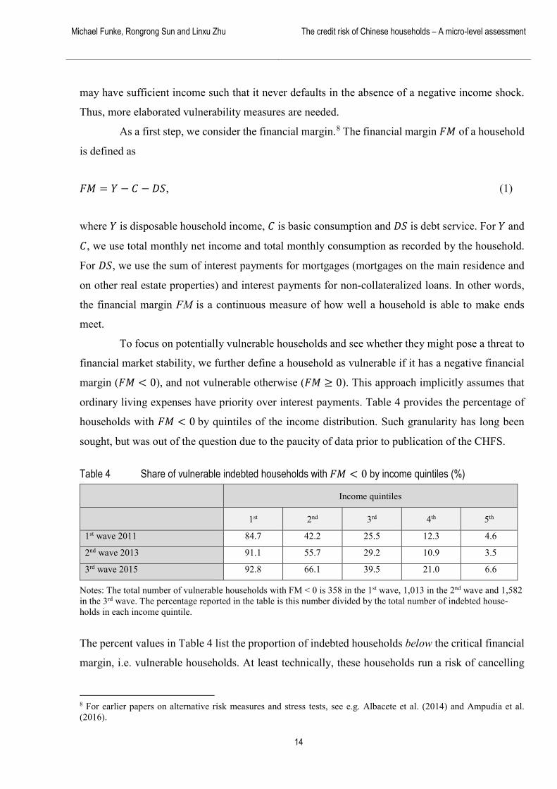
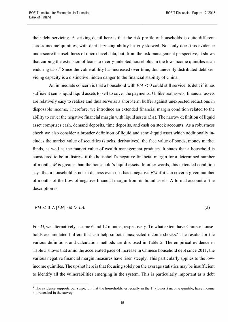
For monitoring purposes, clear presentation and easily interpretation are useful. In this spirit, we
identify vulnerable households by combining the indicators presented above. Our aim here is to
focus on vulnerable households most likely to run into serious problems and cause losses to the
lender. Looking at the joint distribution of the vulnerability indicators gives us a good picture of
households that can be considered “at risk.” To this end, we divide the DA and DSI ratios into six
classes. The first class stands for a DA ratio between 0 and 0.2, and a DSI ratio between 0 and 0.10.
Accordingly, the last class corresponds to a DA ratio above 1 and a DSI ratio above 0.5. The height
of the bars represents the share of households with corresponding DA and DSI ratios. The resulting
(6×6) matrices form the basis for the 3-dimensional vulnerability bar graph. The graph is color coded
BOFIT- Institute for Economies in Transition Bank of Finland
BOFIT Discussion Papers 12/ 2018
17
to differentiate varying risk levels. The dark blue bars represent, broadly speaking, high joint vul-
nerability clusters. Light blue clusters are less vulnerable, while the green, orange and yellow clus-
ters represent increasingly less problematic households.
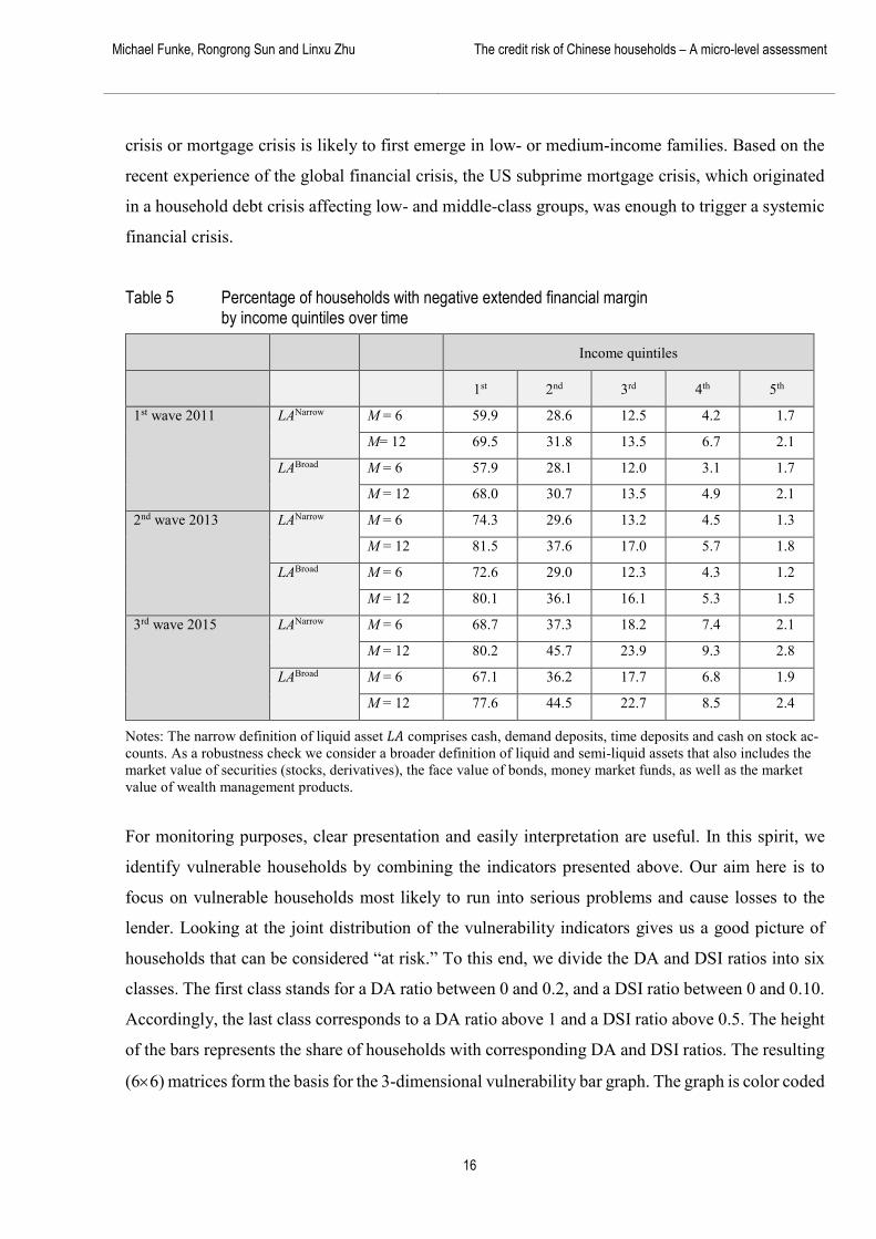
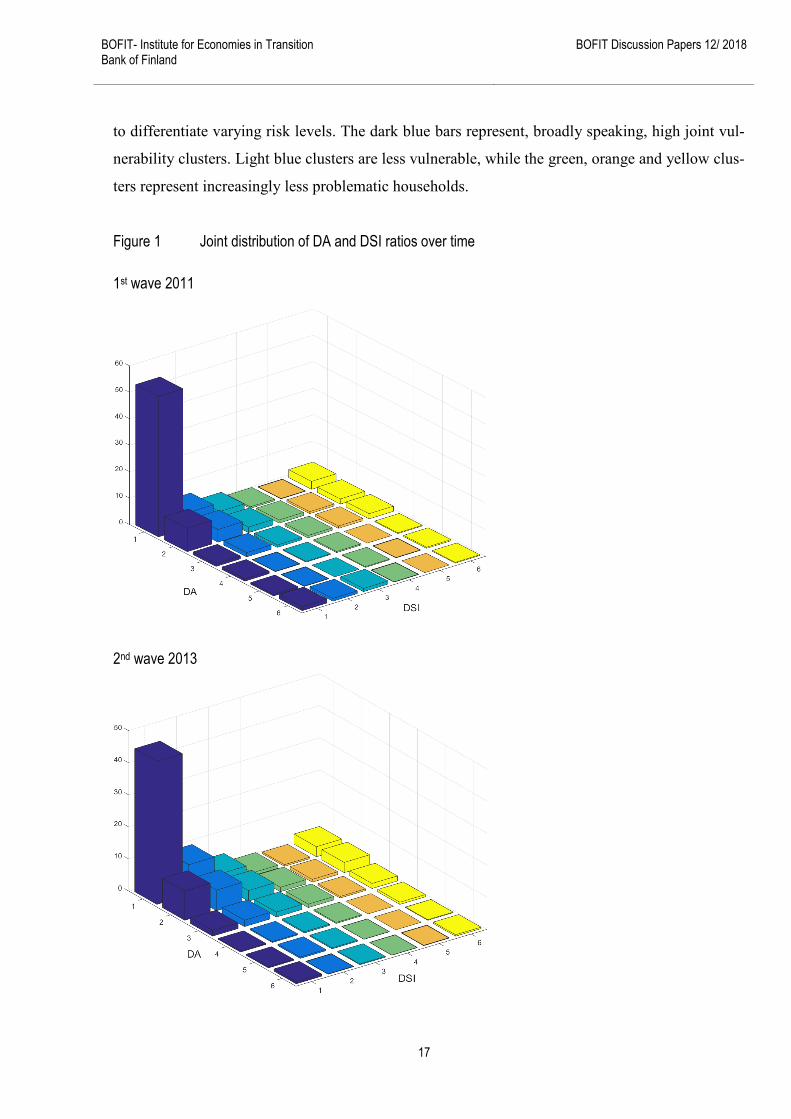
Figure 1 Joint distribution of DA and DSI ratios over time 1st wave 2011
2nd wave 2013

Michael Funke, Rongrong Sun and Linxu Zhu The credit risk of Chinese households – A micro-level assessment
18
3rd wave 2015
The results enable us to identify pockets of credit risk over time. The data show that the financial
standing of households in 2015 deteriorated significantly in comparison to 2011 and 2013. This
result matches the conclusions of the previous sections. Overall, some low-income households ap-
pear to be so heavily indebted that they find it difficult to manage their debt with their own income.
This is important because household-level spending adjustments are more likely to be amplified if
debt is concentrated among households with limited access to credit or with less scope for self-
insurance (see Zabai, 2017). By way of qualification, it must be conceded that, according to the
survey, low-income quintile households should default more frequently on their debts than they
actually do. This supports our suspicion that households, especially in the first quintile, have unre-
ported income or assets not recorded in the survey.
In recent decades, real property has become the de facto store of wealth in China and the
ultimate choice for investors given its high return. In view of the importance of housing in the bal-
ance sheets of households and credit institutions, the final step in this section involves the calcula-
tion of loan-to-value (LTV) ratios.10 While various mortgage debt LTV measures are monitored, we
focus on initial and current LTV ratios. We also distinguish between main residence, second resi-
dence and third residence. The initial LTV ratio is defined by the initial mortgage loan divided by
10 The high growth rate of mortgage debt in China in recent years has captured headlines around the world. For example, Bloomberg ran in 2014 a provocatively title article “Is China Building a Mortgage Bomb?” (https://www.bloom-berg.com/view/articles/2014-11-21/is-china-building-a-mortgage-bomb).

BOFIT- Institute for Economies in Transition Bank of Finland
BOFIT Discussion Papers 12/ 2018
19
the value of the property at the time the mortgage was taken out. In other words, “L” and “V” are
calculated as of loan origination, and not updated afterwards.
Limits on the initial LTV ratio are a popular macroprudential tool to make financial insti-
tutions and households more resilient to house price, income and interest rate shocks.11 By contrast,
the current LTV ratio in the CHFS is defined as the currently outstanding amount of “L” divided by
the self-assessed and updated “V.”12 The LTV is both an indicator of default risk (when calculated
at loan origination) and an indicator of expected loss (when the “V” is updated). Since the updated
“V” gives the estimated foreclosure value, the current LTV ratio is the preferred measure to assess
the current financial stability implication of Chinese household mortgages. The initial LTV ratio is
of interest to macroprudential regulators because it is a predictor of default.13 A high initial LTV
ratio implies higher leverage, and therefore higher risk, i.e. the borrower has been obliged to borrow
more as he or she otherwise could not afford the property. Also, the amount of equity invested in
the house can be used as an indicator of willingness to pay.
From the macroprudential perspective, an LTV ratio tightening may reduce demand for
mortgages as homebuyers are forced out of the property market. An LTV cap tightening may also
reduce credit supply because it may lead banks to lend less than they otherwise would. The focus
upon macroprudential policies reflects the increasing skepticism towards standard monetary policy
in tempering housing booms in support of financial stability. For example, Svensson (2014) argues
the costs of higher interest rates in terms of higher unemployment in Sweden exceed the benefits of
reducing financial stability risks. This implies a costly trade-off of using standard monetary policy
to temper house prices when macroeconomic and financial stability goals are in conflict. While we
cannot do justice to the complete literature, one can point to the work of Arslan et al. (2015), who
show that macroprudential policies help moderate fluctuations in house prices and mortgage default
11 House price growth should be a focus for monitoring and regulatory vigilance. The IMF “Global Housing Watch” (http://www.imf.org/external/research/housing/) traces the evolution and dynamics of house prices in China from an international perspective. A growing literature has documented the use of macroprudential policies including capped LTV ratios across countries and analyzed their effects. Galati and Moessner (2012) provide a review of China’s macro-prudential housing-finance toolkit. Cerutti et al. (2017) document the use of macroprudential policies for 119 countries over the period 2000–2013 that covers many instruments. Recent work on macroprudential policy includes Bianchi et al. (2012, 2016) and Farhi and Werning (2016). 12 LTV ratios may be calculated in several ways. For instance, the market value “V” in LTV may be left unchanged after the loan issuance. This results in conservative LTV estimates when prices rise after loan origination, but can be misleading if house prices decrease. The ratings agency Standard and Poor’s typically uses the lower of the updated price and the original valuation of the property. See https://www.standardandpoors.com/en_US/web/guest/ratings/rat-ings-criteria/-/articles/criteria/structured-finance/filter/rmbs. Given their subjective nature, the self-assessed current market value “V” in the CHFS implies that precise current LTV ratios should be interpreted with caution. 13 The recent literature on the global financial crisis provides ample evidence that the boom was to a large extent driven by an increased willingness by lenders to extend loans to a riskier category of borrowers (Demyanyk and Van Hemert, 2011, Mayer et al., 2009, Mian and Sufi, 2009, Dell’Ariccia et al., 2012).

Michael Funke, Rongrong Sun and Linxu Zhu The credit risk of Chinese households – A micro-level assessment
20
rates. It is well-known that policymakers can only target marginal lending in principle. However,
the intention is that the macroprudential policies should have an effect over the entire life of the
mortgage contract. Therefore, we look at all borrowers, not only those taking new loans.
Table 6 shows the mean initial and current LTV ratios for all three waves and thus monitors
vulnerabilities related to the residential real estate sector in a simple and informative way. In addi-
tion, the LTV ratios for multiple housing owners who have expanded their borrowings in line with
the buoyancy of the Chinese housing market are given.
Table 6 Mean household LTV ratios by income quintiles over time
Income quintiles
1st 2nd 3rd 4th 5th
1st wave 2011 Initial LTV ratio in % Main residence 0.53 0.44 0.49 0.53 0.57
2nd residence 0.75 0.56 0.58 0.55 0.61
3rd residence NA NA NA NA 0.69
Current LTV ratio in % Main residence 0.13 0.12 0.16 0.17 0.20
2nd residence 0.34 0.18 0.24 0.20 0.28
3rd residence NA NA NA NA 0.32
2nd wave 2013 Initial LTV ratio in % Main residence 0.42 0.45 0.46 0.49 0.53
2nd residence 0.69 0.59 0.66 0.57 0.63
3rd residence NA NA NA NA 0.58
Current LTV ratio in % Main residence 0.35 0.31 0.29 0.28 0.39
2nd residence 0.34 0.26 0.35 0.34 0.33
3rd residence NA NA NA NA 0.28
3rd wave 2015 Initial LTV ratio in % Main residence 0.63 0.54 0.55 0.54 0.56
2nd residence NA NA NA NA NA
3rd residence NA NA NA NA NA
Current LTV ratio in % Main residence 0.48 0.57 0.35 0.37 0.40
2nd residence NA NA NA NA NA
3rd residence NA NA NA NA NA
Notes: The main residence is owner-occupied housing. The 2nd and 3rd residences are other properties owned by the household. The table reports the average LTV ratio in each income quintile. NA indicates that the number of observa-tions in that category is less than 5. Please note that in the 3rd wave, mortgage loans are not reported for each individ-ual residence. Rather, total household mortgage loans are reported. Thus, we have only calculated the LTV ratios for those households with one residence. Due to this fact, the data for 2015 are only marginally comparable with earlier figures.
What emerges from this regarding mortgage soundness? In the first instance, the initial LTV ratios
are relatively low compared to other countries (see e.g. Thebault, 2017). Two opposing trends are

BOFIT- Institute for Economies in Transition Bank of Finland
BOFIT Discussion Papers 12/ 2018
21
visible. On one hand, the comparison of the initial and current LTV ratios reveals that rising house
prices and the amortization requirement (minus newly-raised debt) have produced the desired
macroprudential effect, i.e. households decreasing their LTV ratios over the contractual period is a
positive development. This is counteracted, however, by the trend shown in Table 6 that the LTV
ratios are increasing in the 3rd wave. Note that the household risk profile by quantiles of the income
distribution in Table 6 differs substantially from the risk profiles in Table 4 and 5. This underscores
the usefulness of LTV-based measures and can be explained to some extent by self-regulation in the
banking sector related to mortgage credit risk.
Overall, the LTV ratios do not give cause for concern.14 This applies especially to current
LTV ratios. However, asset valuations are procyclical and could fall sharply when the boom ends.
There is also a mismatch in the structure of liabilities and assets. Household liabilities are mostly
financial liabilities, while a significant portion of assets are nonfinancial fixed assets (e.g. housing)
that are illiquid and subject to sharp valuation changes. In addition, more vulnerable households
such as those with lower debt-servicing capacity tend to hold fewer liquid assets, suggesting they
have lower buffers in times of stress.
In concluding this section, we take a closer look at the shift of the current LTV ratio over
time. A convenient way to illustrate the LTV ratio distributions is to calculate univariate kernel
smoothing estimates.
Figure 2 tracks the distribution of LTV ratios over time, and shows that the LTV distribu-
tion has evolved. From 2011 to 2013, the residential mortgage loan LTV ratios increased modestly.
From 2013 to 2015, the data show a surge in the LTV ratios. Nonetheless, it should be emphasized
that appreciating Chinese house prices in the observation period were not accompanied by an ex-
ceptionally rapid increase in current LTV ratios. This finding contrasts with the situation in many
advanced economies prior to the global financial crisis.
14 Chinese savings behavior could also be a factor. Chinese households save more at every income decile than in other countries, but the gap is largest for the poor (see IMF, 2017c, pp. 7-11). The exceptional consumption-saving pattern in China is influenced by precautionary saving motives to a considerable extent (Chamon and Prasad, 2010, and Chamon et al., 2013). It should also be noted that informal borrowing among friends and relatives is prevalent in China. In the second wave of the CHFS in 2013, over 30% of homebuyers in China informally borrowed from friend and relatives. The average amount borrowed from friends and family was RMB 70,000, and the average reported interest rate of informal borrowing was 0.4%.

Michael Funke, Rongrong Sun and Linxu Zhu The credit risk of Chinese households – A micro-level assessment
22
Figure 2 Distributions of current LTV ratios for main residence over time
4 Stress tests As a first step, we present and explain the methodology that underpins the stress index. Stress tests
raise two questions: where do the adverse shocks occur and what is their magnitude? Below we
conduct micro-simulations with income and house price changes and assess the associated picture
of vulnerabilities.15 In doing so, we assume that both shocks are independent from each other. The
guiding principle underpinning the stress tests is that future shocks hitting the Chinese economy are
inherently unpredictable.16 But if and when shocks materialize, their impact should vary according
to exposures and leverage built up in the system. Unlike actual shocks, these vulnerabilities can be
assessed and monitored. To this end, we conduct stress tests reflecting different risk factors.
We start by monitoring the resilience of households under adverse income shocks employ-
ing the 𝐹𝐹𝐹𝐹 < 0 cut-off in equation (1). The results are given in Table 7. The income shock is mod-
elled via a uniform reduction of income 𝑌𝑌 of all households. We calculate the static impact effects
15 The predominant mortgage contract in China is an adjustable-rate mortgage (Zabai, 2017, p. 42). As a result, one might assume an interest rate shock. In practice, however, Chinese policymakers are most likely to leave the benchmark interest rate unchanged amid reasonable CPI inflation rises and a stable renminbi – even with the current likelihood of rising US interest rates. The People’s Bank of China intends to keep its monetary policy independent and the current CPI inflation provides no incentive to take further steps. Thus, our stress test design seems appropriate for the questions posed here. 16 The focus on unexpected shocks prevents a rigorous assessment of anticipated macroeconomic shocks or economic policy changes. This drawback cannot be ignored.
BOFIT- Institute for Economies in Transition Bank of Finland
BOFIT Discussion Papers 12/ 2018
23
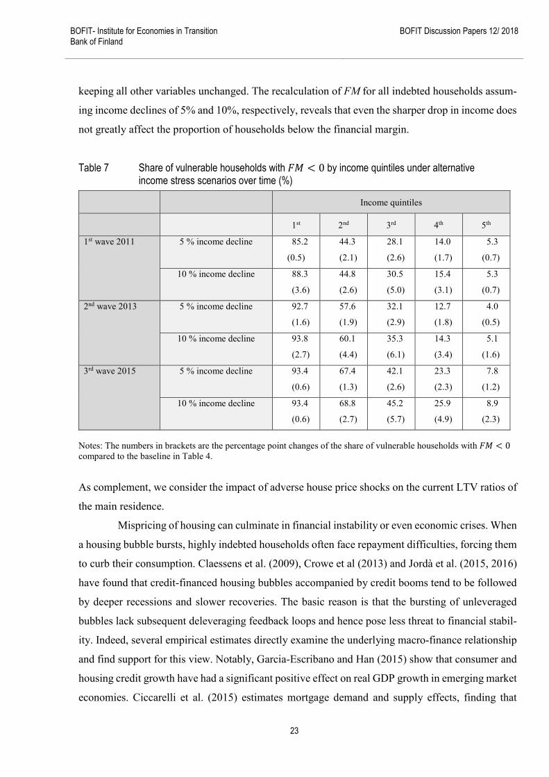
keeping all other variables unchanged. The recalculation of FM for all indebted households assum-
ing income declines of 5% and 10%, respectively, reveals that even the sharper drop in income does
not greatly affect the proportion of households below the financial margin.
Table 7 Share of vulnerable households with 𝐹𝐹𝐹𝐹 < 0 by income quintiles under alternative income stress scenarios over time (%)
Income quintiles
1st 2nd 3rd 4th 5th
1st wave 2011 5 % income decline 85.2
(0.5)
44.3
(2.1)
28.1
(2.6)
14.0
(1.7)
5.3
(0.7)
10 % income decline 88.3
(3.6)
44.8
(2.6)
30.5
(5.0)
15.4
(3.1)
5.3
(0.7)
2nd wave 2013 5 % income decline 92.7
(1.6)
57.6
(1.9)
32.1
(2.9)
12.7
(1.8)
4.0
(0.5)
10 % income decline 93.8
(2.7)
60.1
(4.4)
35.3
(6.1)
14.3
(3.4)
5.1
(1.6)
3rd wave 2015 5 % income decline 93.4
(0.6)
67.4
(1.3)
42.1
(2.6)
23.3
(2.3)
7.8
(1.2)
10 % income decline 93.4
(0.6)
68.8
(2.7)
45.2
(5.7)
25.9
(4.9)
8.9
(2.3)
Notes: The numbers in brackets are the percentage point changes of the share of vulnerable households with 𝐹𝐹𝐹𝐹 < 0 compared to the baseline in Table 4.
As complement, we consider the impact of adverse house price shocks on the current LTV ratios of
the main residence.
Mispricing of housing can culminate in financial instability or even economic crises. When
a housing bubble bursts, highly indebted households often face repayment difficulties, forcing them
to curb their consumption. Claessens et al. (2009), Crowe et al (2013) and Jordà et al. (2015, 2016)
have found that credit-financed housing bubbles accompanied by credit booms tend to be followed
by deeper recessions and slower recoveries. The basic reason is that the bursting of unleveraged
bubbles lack subsequent deleveraging feedback loops and hence pose less threat to financial stabil-
ity. Indeed, several empirical estimates directly examine the underlying macro-finance relationship
and find support for this view. Notably, Garcia-Escribano and Han (2015) show that consumer and
housing credit growth have had a significant positive effect on real GDP growth in emerging market
economies. Ciccarelli et al. (2015) estimates mortgage demand and supply effects, finding that

Michael Funke, Rongrong Sun and Linxu Zhu The credit risk of Chinese households – A micro-level assessment
24
changes in demand significantly affect GDP growth. In countries where post-crisis deleveraging did
not put downward pressure on household loan demand, sustained household consumption expendi-
ture and housing investment act to stabilize economic growth.
On the other hand, international experience suggests that housing booms are dangerous.
They increase the risk of a disruptive adjustment, a marked growth slowdown, or both. Forced asset
sales (fire sales) can also aggravate financial fragility by depleting the balance sheets of market
participants. Fire sales imply discounts below fundamental values, with market conditions and the
urgency of the sale determining the amount of the fire sale discount. Discounts are larger in thin
markets with low demand. Fire sales are more likely under of financial or liquidity constraints.17
Fire sales also may generate externalities that feedback on asset values, thereby magnifying finan-
cial accelerator effects and causing price-default spirals.18
A separate risk factor is reassessment of the future monetary policy stance. The resulting
snapback in bond yields and the initial price correction may be magnified by fire sales. Conse-
quently, the macroprudential authority should as a precaution pay close attention to signs of exces-
sive house prices.
Quantitative plain-vanilla risk metrics are presented in Table 8. As a double check, we look
at 10% and 25% house price drops. These house price discounts are meant to account for fire sale
risks, property specific features and legal/transaction costs. Again, we calculate the impact effects
ceteris paribus.
Table 8 suggests that the current LTV ratios were only mildly sensitive to house price
shocks in all three waves. Thus, Chinese households facing affordability problems do not seem
particularly vulnerable to declining house prices and are unlikely to experience long-term mortgage
arrears or sharp contractions in spending. Indeed, even a house price decline of 25% is unlikely to
trigger a systemic impact on the Chinese financial sector.
17 For a review of the literature and possibility of fire sales externalities, see Shleifer and Vishny (2011), Caballero and Simsek (2013) and Choi and Cook (2012). 18 The collapse of US housing prices in 2007–2010 was followed by a dramatic increase in mortgage defaults that often led to foreclosures. Empirical evidence supports for this feedback loop conjecture. See Campbell et al. 2011), Elul et al. (2010) and Harding et al. (2010).

BOFIT- Institute for Economies in Transition Bank of Finland
BOFIT Discussion Papers 12/ 2018
25
Table 8 Mean of the current main residence LTV ratios in percent by income quintiles over time under alternative house price decline scenarios
Income quintiles
1st 2nd 3rd 4th 5th
1st wave 2011 10 % house price decline 0.14 0.13 0.18 0.19 0.22
25 % house price decline 0.17 0.16 0.21 0.23 0.27
2nd wave 2013 10 % house price decline 0.39 0.34 0.32 0.32 0.44
25 % house price decline 0.46 0.41 0.39 0.38 0.52
3rd wave 2015 10 % house price decline 0.46 0.63 0.39 0.41 0.45
25 % house price decline 0.51 0.76 0.47 0.49 0.54
Note: For convenience, we assume house prices decreased by the same amount at the same time throughout China.
We have not tied up all issues in this section. Notably, the above stress tests are partial equilibrium
analyses and do not account for the economic interactions between the various markets in a given
economy. This would require a general equilibrium setup where all markets are simultaneously
modelled and interact with each other. Even so, due to their robustness to misspecification in other
parts of the economy, easy-to-implement partial equilibrium models are well justified. An obvious
advantage of partial equilibrium models is that they break the task of figuring out how the world
works into manageable pieces. Moreover, besides the wealth of empirical detail, partial equilibrium
modelling is often the preferred initial strategy to figure out, piece by piece, the effects of policies
and shocks. As a general comment, there are advantages and disadvantages of each modelling ap-
proach.19
5 Conclusions and discussion The global financial crisis has brought the international analysis of risks and vulnerabilities to the
fore. Using a micro-level lens, the objective of this work has been to clarify detail in the evolution
19 Of course, addressing financial stability challenges with intertemporal implications requires structural models as a next step. It is not enough to rely on micro-level empirical evidence. In his famous critique of the empirical characteri-zation of business cycles of Burns and Mitchell (1946), Koopmans (1947) articulated the limited nature of conclusions that follow measurement without theory. Thus, extension of the present modelling approach with a view to optimizing behavior and policies holds potential as a subject for future research. The development of Heterogeneous Agent New Keynesian (HANK) models have helped (see Ahn et al., 2018 and Kaplan et al., 2018), but we are far from a clear understanding. In the meantime, assessments that meet prudential requirements must rely primarily on careful statistical analysis of the data.

Michael Funke, Rongrong Sun and Linxu Zhu The credit risk of Chinese households – A micro-level assessment
26
of financial vulnerabilities. Our identification of vulnerabilities employed is in line with the previ-
ous, somewhat sparse, micro-level literature on the topic. We add to the literature by looking at a
broad set of variables for measuring vulnerabilities, and, to our best knowledge, provide the first
such analysis focused exclusively on China.
The three published waves of the China Household Finance Survey fill a void in infor-
mation on household finances in China. They provide unrivalled insights into household balance
sheet data over the entire income distribution and allow us to address topical policy issues under the
microscope where information from other sources is less meaningful. The GHFS is also useful, as
shown above, in addressing distributional issues. Combining all relevant pieces of information, the
empirical monitoring approach presented in this paper enables an accurate diagnostic of the debt
vulnerability of households and thus is a useful complement of macroeconomic model-based tools
for analyzing the build-up of financial imbalances and vulnerabilities.20
We can offer no overarching key message; our evidence draws a mixed picture on house-
hold indebtedness and financial vulnerability. LTV ratios generally are safe and sound, but many
Chinese households in the lowest income quintiles face great vulnerability and seem hard-pressed
to meet their debt commitments over the short, medium and long term. From the perspective of
financial stability, the participation of low income households in the debt market is below average,
mitigating the impact of their eventual default on the financial situation of affected banks.
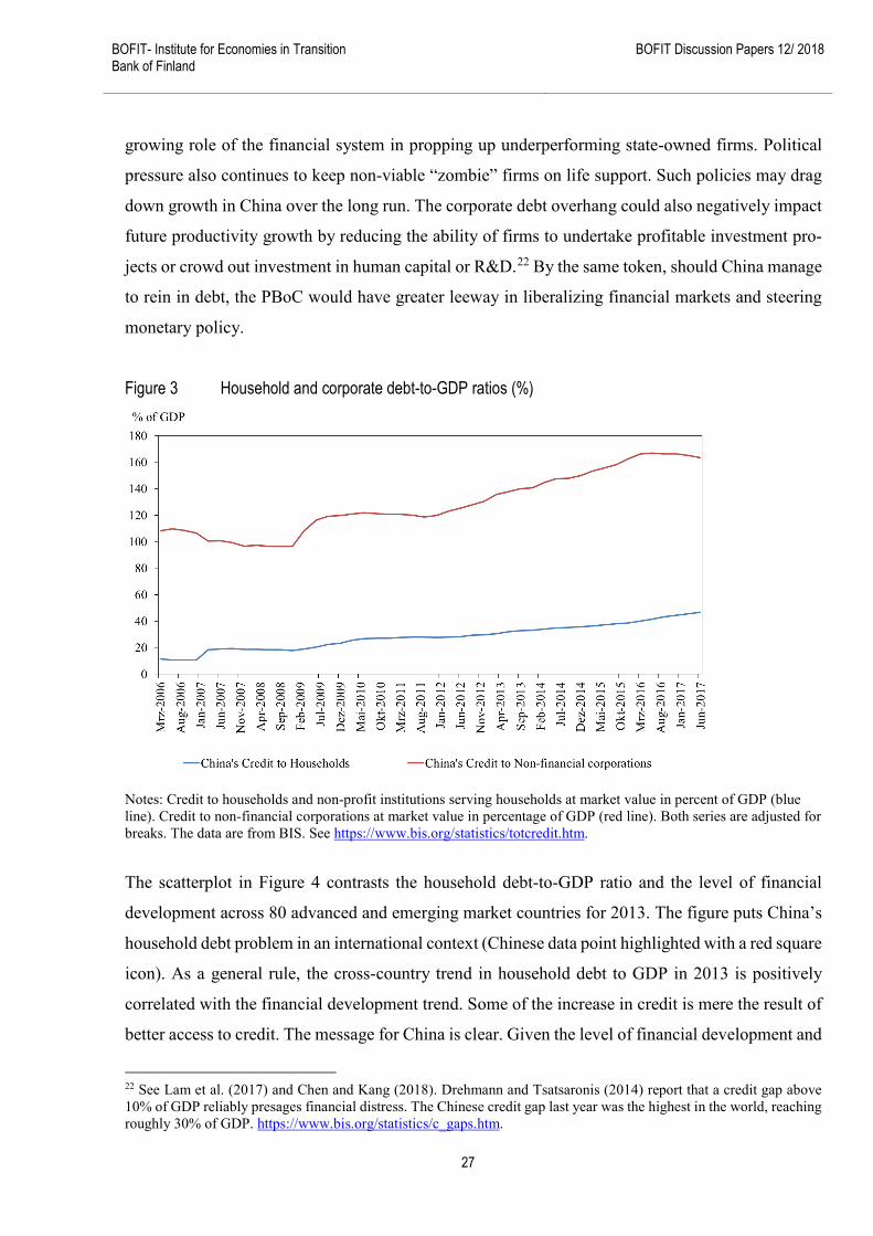
Surveys, of course, take no long-term view and suffer from publication lags. In order to
provide a longer-term macroeconomic view to complement this analysis, Figure 3 presents China’s
household and corporate credit-to-GDP ratios from 2006 to 2017. Historical experience shows that
household debt to GDP in China averaged 11.5% of GDP in March 2006 and reached an all-time
high of 46.8% of GDP in June 2017. In other words, China’s household debt-to-GDP ratio quadru-
pled between 2006 and 2017. It is this build-up of household debt that has sparked widespread
concern about the health and vulnerability of the Chinese economy.21
We should keep in mind that Chinese household debt started from an extremely low base.
Furthermore, China’s big problem is corporate debt. The corporate debt-to-GDP ratio reflects the
20 Aggravating this long-term concomitant effect, Danielsson and Zhou (2016) and Danielsson et al. (2016) have argued that model-based monitoring approaches do not necessarily offer the best guidance during market distress and may not reveal risks which could have been shown by simple metrics. 21 See https://www.bloomberg.com/news/articles/2017-11-21/china-s-debt-surge-may-increase-risk-of-financial-crisis. Chinese policymakers are well aware of the potential risks of high GDP growth projections in national plans. See https://www.bloomberg.com/news/articles/2017-10-19/zhou-warns-china-should-defend-against-threat-of-minsky-moment. Comparison of Table 3 and Figure 3 also shows the extent to which the aggregate macroeconomic household debt ratio underestimates the actual burden of debt of indebted households.
BOFIT- Institute for Economies in Transition Bank of Finland
BOFIT Discussion Papers 12/ 2018
27
growing role of the financial system in propping up underperforming state-owned firms. Political
pressure also continues to keep non-viable “zombie” firms on life support. Such policies may drag
down growth in China over the long run. The corporate debt overhang could also negatively impact
future productivity growth by reducing the ability of firms to undertake profitable investment pro-
jects or crowd out investment in human capital or R&D.22 By the same token, should China manage
to rein in debt, the PBoC would have greater leeway in liberalizing financial markets and steering
monetary policy.
Figure 3 Household and corporate debt-to-GDP ratios (%)
Notes: Credit to households and non-profit institutions serving households at market value in percent of GDP (blue line). Credit to non-financial corporations at market value in percentage of GDP (red line). Both series are adjusted for breaks. The data are from BIS. See https://www.bis.org/statistics/totcredit.htm.
The scatterplot in Figure 4 contrasts the household debt-to-GDP ratio and the level of financial
development across 80 advanced and emerging market countries for 2013. The figure puts China’s
household debt problem in an international context (Chinese data point highlighted with a red square
icon). As a general rule, the cross-country trend in household debt to GDP in 2013 is positively
correlated with the financial development trend. Some of the increase in credit is mere the result of
better access to credit. The message for China is clear. Given the level of financial development and
22 See Lam et al. (2017) and Chen and Kang (2018). Drehmann and Tsatsaronis (2014) report that a credit gap above 10% of GDP reliably presages financial distress. The Chinese credit gap last year was the highest in the world, reaching roughly 30% of GDP. https://www.bis.org/statistics/c_gaps.htm.

Michael Funke, Rongrong Sun and Linxu Zhu The credit risk of Chinese households – A micro-level assessment
28
sophistication, China’s household debt in 2013 was not unreasonably high. Thus, the macro-level
evidence broadly corroborates the micro-level assessment presented above.
Figure 4 China’s household debt problem in a financial development context
Notes: See IMF (2017a), Figure 2.3, p. 60. The financial development index is taken from Svirydzenka (2016). For the list of advanced and emerging market economies included, see IMF (2017a), p. 81.
This paper surveyed potential concerns for financial stability, echoing the increased scrutiny of Chi-
nese household debt in the media and by regulators. But is household debt a ticking time bomb?
Based on our household-level analysis, we argue that there exists a substantial margin of safety and
thus a strongly pessimistic outlook regarding household debt in China probably misses the mark.
Instead, we would argue that policymakers take a nuanced view.
Of course, China’s debt situation warrants careful monitoring, particularly with regard to
lower income brackets. In addition, further financial reforms are needed to bolster the regulatory
and supervisory framework, and increasing transparency of nonbank financial institutions and
wealth management products.23 Good policies, institutions and regulations make a difference. For
example, countries with floating exchange rates, and which are financially more developed, are
better placed to weather the consequences of high household debt (Dell’Ariccia et al., 2016 and
IMF, 2017a). Future work should thus attempt to identify general conditions that might improve
financial resilience. We anticipate that therein lies promising potential for future research.
23 Policymakers may wait to see whether increasing household debt reflects a genuine economic trend or is just a statis-tical blip. Even when they act, macroprudential tools take time to have an effect.

BOFIT- Institute for Economies in Transition Bank of Finland
BOFIT Discussion Papers 12/ 2018
29
References Ahn, S., G. Kaplan, B. Moll, T. Winberry and C. Wolf (2018). “When Inequality Matters for
Macro and Macro Matters for Inequality,” NBER Macroeconomics Annual (forthcoming). Albacete, N., J. Eidenberger, G. Krenn, P. Lindner, and M. Sigmund (2014). “Risk-Bearing Ca-
pacity of Households – Linking Micro-Level Data to the Macroprudential Toolkit,” Aus-trian National Bank Financial Stability Report 27, June, 95–110.
Ampudia, M., H. van Vlokhoven and D. Żochowski (2016). “Financial Fragility of Euro Area Households,” Journal of Financial Stability 27, 250–262.
Arslan, Y., B. Guler and T. Taskin (2015). “Joint Dynamics of House Prices and Foreclosures,” Journal of Money, Credit and Banking 47, 133–169.
Bianchi, J., E. Boz and E.G. Mendoza (2012). “Macroprudential Policy in a Fisherian Model of Financial Innovation,” IMF Economic Review 60, 223–269.
Bianchi, J., C. Liu, and E.G. Mendoza (2016). “Fundamentals News, Global Liquidity and Macro-prudential Policy,” Journal of International Economics 99 (supplement), S2–S15.
Bracke, P. and H. Sethi (2017). “The Financial Position of British Households: Evidence from the 2017 NMG Consulting Survey,” Bank of England Quarterly Bulletin 2017/Q4, 1–11. Bricker, J., B. Bucks, A.B. Kennickell, T.L. Mach and K. Moore (2015). “Drowning or Weathering
the Storm? Changes in Family Finances from 2007 to 2009,” in: Hulten, C.R. and M.B. Reinsdorf (eds.) Measuring Wealth and Financial Intermediation and Their Links to the Real Economy, Chicago (University of Chicago Press), 323–348.
Burns, A.F. and W.C. Mitchell (1946). Measuring Business Cycles, Cambridge (National Bureau of Economic Research).
Caballero, R.J. and A. Simsek (2013). “Fire Sales in a Model of Complexity,” Journal of Finance 68, 2549–2587.
Campbell, J.Y, S. Giglio and P. Pathak (2011). “Forced Sales and House Prices,” American Eco-nomic Review 101, 2108–2131.
Cerutti, E., S. Claessens and L. Laeven (2017). “The Use and Effectiveness of Macroprudential Policies: New Evidence,” Journal of Financial Stability 28, 203–224.
Chamon, M.D. and E.S. Prasad (2010). “Why are Saving Rates of Urban Households in China Rising?” American Economic Journal: Macroeconomics 2, 93–130.
Chamon, M.D., K. Liu and E.S. Prasad (2013). “Income Uncertainty and Household Savings in China,” Journal of Development Economics 105, 164–177.
Chen, S. and J.S. Kang (2018). “Credit Booms – Is China Different?” IMF Working Paper No. WP/18/2, Washington DC.
Choi, W.G. and D. Cook (2012). “Fire Sales and the Financial Accelerator,” Journal of Monetary Economics 59, 336–351.
Ciccarelli, M., A. Maddaloni and J. Peydró (2015). “Trusting the Bankers: A New Look at the Credit Channel of Monetary Policy,” Review of Economic Dynamics 18, 979–1002.
Michael Funke, Rongrong Sun and Linxu Zhu The credit risk of Chinese households – A micro-level assessment
30
Claessens, S., M. Kose and M. Terrones (2009). “What Happens During Recessions, Crunches and Busts?” Economic Policy 24(60), 653–700.
Crowe, C., G. Dell’Ariccia, D. Igan and P. Rabanal (2013). “How to Deal with Real Estate Booms: Lessons from Country Experiences,” Journal of Financial Stability 9, 300–319.
Danielsson, J. and C. Zhou (2016). “Why risk is so hard to measure,” De Nederlandsche Bank Working Paper No. 494, Amsterdam.
Danielsson, J., K.R. James, M. Valenzuela and I. Zer (2016) “Model Risk of Risk Models,” Jour-nal of Financial Stability 23, 79–91.
Dell’Ariccia, G., D. Igan and L. Laeven (2012). “Credit Booms and Lending Standards: Evidence from the Subprime Mortgage Market,” Journal of Money, Credit and Banking 44, 367-384.
Dell’Ariccia, G., D. Igan, L. Laeven and H. Tong (2016). “Credit Booms and Macrofinancial Sta-bility,” Economic Policy 31, 299–355.
Demyanyk, Y.S. and O. Van Hemert (2011). “Understanding the Subprime Mortgage Crisis,” Re-view of Financial Studies 24, 1848–1880.
Djoudad, R. (2012). “A Framework to Assess Vulnerabilities Arising from Household Indebted-ness
Using Microdata,” Bank of Canada Discussion Paper No. 2012–3, Ottawa. Drehmann, M. and M. Juselius (2012). “Do Debt Service Costs Affect Macroeconomic and Fi-
nancial Stability?” BIS Quarterly Review, September, 21–35. Drehmann, M., M. Juselius and A. Korinek (2017). “Accounting for Debt Service: The Painful
Legacy of Credit Booms,” BIS Working Paper No. 645, Basel. Drehmann, M. and K. Tsatsaronis (2014). “The Credit-to-GDP Gap and Countercyclical Capital
Buffers: Questions and Answers,” BIS Quarterly Review, March, 55–73. ECB (2013). Financial Stability Review, November 2013, Frankfurt. Elul, R. (2008). “Collateral, Credit History, and the Financial Decelerator,” Journal of Financial
Intermediation 17, 63–88. Elul, R., N. Souleles, S. Chomsisengphet, D. Glennon and R. Hunt (2010). “What ‘Triggers’ Mort-
gage Default,” American Economic Review 100, 490–494. Farhi, E. and I. Werning (2016). “A Theory of Macroprudential Policies in the Presence of Nom-
inal Rigidities,” Econometrica 84, 1645–1704. Galati, G. and R. Moessner (2012). “Macroprudential Policy – A Literature Review,” Journal of
Economic Surveys 27, 846–878. Gan, L., Z. Yin, N. Jia, S. Xu, S. Ma, S. and L. Zheng (2014). Data you need to know about China.
Research Report of China Household Finance Survey 2012, New York (Springer). Garcia-Escribano, M. and F. Han (2015). “Credit Expansion in Emerging Markets: Propeller of
Growth?” IMF Working Paper WP/15/212, Washington DC. Harding, J.P., E. Rosenblatt, and V.W. Yao (2008). “The Contagion Effect of Foreclosed Proper-
ties,” Journal of Urban Economics 66, 164–178. IMF (2012). “Spain: Vulnerabilities of Private Sector Balance Sheets and Risks to the Financial
Sector,” IMF Country Report No. 12/140, Washington DC.
BOFIT- Institute for Economies in Transition Bank of Finland
BOFIT Discussion Papers 12/ 2018
31
IMF (2017a). Global Financial Stability Report, October, Washington DC. IMF (2017b). People’s Republic of China – Financial System Stability Assessment, Washington
DC. IMF (2017c). People’s Republic of China – Selected Issues, Washington DC. Jordà, Ò, M. Schularick and A.M. Taylor (2015). “Leveraged Bubbles,” Journal of Monetary Eco-
nomics 76 (supplement), S1–S20. Jordà, Ò, M. Schularick and A.M. Taylor (2016). “The Great Mortgaging: Housing Finance, Crises
and Business Cycles,” Economic Policy 31, 107–152. Juselius, M. and M. Drehmann (2015). “Leverage Dynamics and the Real Burden of Debt,” BIS
Working Paper No. 501, Basel. Kaplan, G., B. Moll and G.L. Violante (2018). “Monetary Policy According to HANK,” American
Economic Review (forthcoming). Koopmans, T.C. (1947). “Measurement Without Theory,” Review of Economics and Statistics 29,
161–172. Lam, W.R., A. Schipke, Y. Tan and Z. Tan (2017). “Resolving China’s Zombies: Tackling Debt
and Raising Productivity,” IMF Working Paper WP/17/266, Washington DC. Law, S.H. and N. Singh (2014). “Does Too Much Finance Harm Economic Growth?” Journal of
Banking and Finance 41, 36–44. Martin, P. and T. Philippon (2017). “Inspecting the Mechanism: Leverage and the Great Recession
in the Eurozone,” American Economic Review 107, 1904–1937. Mayer, C., K.M. Pence and S.M. Sherlund (2009). “The Rise in Mortgage Defaults,” Journal of
Economic Perspectives 23, 27–50. Mian, A. and A. Sufi (2009). “The Consequences of Mortgage Credit Expansion: Evidence from
the US Mortgage Default Crisis,” Quarterly Journal of Economics 124, 1449–1496. Mian, A. and A. Sufi (2018). “Finance and Business Cycles: The Credit-Driven Household De-
mand Channel,” NBER Working Paper No. 24322, Cambridge (Mass.). Mian, A.R., A. Sufi and E. Verner (2017). “Household Debt and Business Cycles Worldwide,”
Quarterly Journal of Economics 132, 1755–1817. Reinhart, C.M. and K.S. Rogoff (2009). This Time is Different – Eight Centuries of Financial
Folly, Princeton (Princeton University Press). Shleifer, A. and R. Vishny (2011). “Fire Sales in Finance and Macroeconomics,” Journal of Eco-
nomic Perspectives 25, 29–48. Svensson, L.E.O. (2014). “Inflation Targeting and ‘Leaning against the Wind’,” International
Journal of Central Banking 10, 103–114. Svirydzenka, K. (2016). “Introducing a New Broad-Based Index of Financial Development,” IMF
Working Paper WP/16/5, Washington, DC. Thebault, L. (2017). “The ‘V’ in LTV and why it matters,” European DataWarehouse, Frankfurt,
(reprinted in EMF Hypostat 2017, European Mortgage Federation, September 2017). Zabai, A. (2017). “Household Debt: Recent Developments and Challenges,” BIS Quarterly Re-
view, December, 39–54.
BOFIT Discussion Papers A series devoted to academic studies by BOFIT economists and guest researchers. The focus is on works relevant for economic policy and economic developments in transition / emerging economies.
BOFIT Discussion Papers http://www.bofit.fi/en • email: [email protected]
ISSN 1456-4564 (print) // ISSN 1456-5889 (online)
2017 No 1 Koen Schoors, Maria Semenova and Andrey Zubanov: Depositor discipline in Russian regions: Flight to familiarity or trust in local authorities? No 2 Edward J. Balistreri, Zoryana Olekseyuk and David G. Tarr: Privatization and the unusual case of Belarusian accession to the WTO No 3 Hongyi Chen, Michael Funke, Ivan Lozev and Andrew Tsang: To guide or not to guide? Quantitative monetary policy tools and macroeconomic dynamics in China No 4 Soyoung Kim and Aaron Mehrotra: Effects of monetary and macroprudential policies – evidence from inflation targeting economies in the Asia-Pacific region and potential implications for China No 5 Denis Davydov, Zuzana Fungáčová and Laurent Weill: Cyclicality of bank liquidity creation No 6 Ravi Kanbur, Yue Wang and Xiaobo Zhang: The great Chinese inequality turnaround No 7 Yin-Wong Cheung, Cho-Hoi Hui and Andrew Tsang: The Renminbi central parity: An empirical investigation No 8 Chunyang Wang: Crony banking and local growth in China No 9 Zuzana Fungáčová and Laurent Weill: Trusting banks in China No 10 Daniela Marconi: Currency co-movements in Asia-Pacific: The regional role of the Renminbi No 11 Felix Noth and Matias Ossandon Busch: Banking globalization, local lending, and labor market effects: Micro-level evidence from Brazil No 12 Roman Horvath, Eva Horvatova and Maria Siranova: Financial development, rule of law and wealth inequality: Bayesian model averaging evidence No 13 Meng Miao, Guanjie Niu and Thomas Noe: Lending without creditor rights, collateral, or reputation – The “trusted-assistant” loan in 19th century China No 14 Qing He, Iikka Korhonen and Zongxin Qian: Monetary policy transmission with two exchange rates and a single currency: The Chinese experience No 15 Michael Funke, Julius Loermann and Andrew Tsang: The information content in the offshore Renminbi foreign-exchange option market: Analytics and implied USD/CNH densities No 16 Mikko Mäkinen and Laura Solanko: Determinants of bank closures: Do changes of CAMEL variables matter? No 17 Koen Schoors and Laurent Weill: Russia's 1999-2000 election cycle and the politics-banking interface No 18 Ilya B. Voskoboynikov: Structural change, expanding informality and labour productivity growth in Russia No 19 Heiner Mikosch and Laura Solanko: Should one follow movements in the oil price or in money supply? Forecasting quarterly GDP growth in Russia with higher-frequency indicators No 20 Mika Nieminen, Kari Heimonen and Timo Tohmo: Current accounts and coordination of wage bargaining No 21 Michael Funke, Danilo Leiva-Leon and Andrew Tsang: Mapping China’s time-varying house price landscape No 22 Jianpo Xue and Chong K. Yip: One-child policy in China: A unified growth analysis
2018 No 1 Zheng (Michael) Song and Wei Xiong: Risks in China’s financial system No 2 Jennifer N. Carpenter, Fangzhou Lu and Robert F. Whitelaw: The real value of China’s stock market No 3 Bing Xu: Permissible collateral and access to finance: Evidence from a quasi-natural experiment No 4 Stefan Angrick and Naoyuki Yoshino: From window guidance to interbank rates. Tracing the transition of monetary policy in Japan and China No 5 Veronika Belousova, Alexander Karminsky and Ilya Kozyr: Bank ownership and profit efficiency of Russian banks No 6 Chengsi Zhang and Chao Dang: Is Chinese monetary policy forward-looking? No 7 Israel Marques II: Firms and social policy preferences under weak institutions: Evidence from Russia No 8 Ivan Lyubimov, Margarita Gvozdeva and Maria Lysyuk: Towards increased complexity in Russian regions: networks, diversification and growth No 9 Jeannine Bailliu, Xinfen Han, Mark Kruger, Yu-Hsien Liu and Sri Thanabalasingam: Can media and text analytics provide insights into labour market conditions in China? No 10 Sanna Kurronen: Oil price collapse and firm leverage in resource-dependent countries No 11 Marlene Amstad, Huan Ye and Guonan Ma: Developing an underlying inflation gauge for China No 12 Michael Funke, Rongrong Sun and Linxu Zhu: The credit risk of Chinese households – A micro-level assessment


