

Boston University School of Law Boston University School of Law
Scholarly Commons at Boston University School of Law Scholarly Commons at Boston University School of Law
Faculty Scholarship
3-2018
Automation and Jobs: When Technology Boosts Employment Automation and Jobs: When Technology Boosts Employment
James Bessen
Follow this and additional works at: https://scholarship.law.bu.edu/faculty_scholarship
Part of the Labor and Employment Law Commons, and the Science and Technology Law Commons

AUTOMATION AND JOBS: WHEN TECHNOLOGY BOOSTS EMPLOYMENT
Boston University School of Law Law & Economics Paper No. 17-09
revised March 2018
James BessenBoston University School of Law
This paper can be downloaded without charge at:
http://www.bu.edu/law/faculty-scholarship/working-paper-series/
1
Automation and Jobs:
When Technology Boosts Employment
By James Bessen, Boston University School of Law
March, 2018
Abstract: Do industries shed jobs when they adopt new labor-saving technologies? Sometimes productivity-enhancing technology increases industry employment instead. In manufacturing, jobs grew along with productivity for a century or more; only later did productivity gains bring declining employment. What changed? Markets became saturated. While the literature on structural change provides reasons for the decline in the manufacturing share of employment, few papers can explain both the rise and subsequent fall. Using two centuries of data, a simple model of demand accurately explains the rise and fall of employment in the US textile, steel, and automotive industries. The model helps explain why the Industrial Revolution was highly disruptive despite low productivity growth and why information technologies appear to have positive effects on employment today. JEL codes: J2, O3, N10 Keywords: Automation, technical change, sectoral growth, labor demand, manufacturing, deindustrialization Thanks for helpful comments from Philippe Aghion, David Autor, Claude Diebolt, Martin Fleming, Richard Freeman, Ricardo Hausman, Mike Meurer, Joel Mokyr, Bob Rowthorn, Anna Salomons and participants at the ASSA and the SBBI and CID seminars at Harvard.

2
When an industry automates its production does its employment decline? There is
widespread concern today that many jobs will be lost to new computer technologies. One
recent paper concluded that new information technologies will put “a substantial share of
employment, across a wide range of occupations, at risk in the near future” (Frey and
Osborne 2013).
The example of manufacturing decline provides good reason to be concerned about
technology and job losses. In 1958, the US broadwoven textile industry employed over 300
thousand production workers and the primary steel industry employed over 500 thousand.
By 2011, broadwoven textiles employed only 16 thousand and steel employed only 100
thousand production workers.1 Some of these losses can be attributed to trade, especially
since the mid-1990s. However, overall since the 1950s in developed economies, most of the
decline in manufacturing employment appears to come from technology and changing
demand (Rowthorn and Ramaswamy 1999). Of course, jobs lost in one industry may be
replaced with new jobs in another, but many fear that deindustrialization has heightened
economic inequality in the US or caused unemployment in Europe and caused political
instability in both. “Premature deindustrialization” has also become a concern in developing
nations (Rodrik 2016).
Yet technical change does not always lead to declining employment in the affected
industry. Figure 1 shows how textiles, steel, and automotive manufacturing all enjoyed
strong employment growth during many decades that also experienced very rapid
productivity growth. This “inverted U” pattern appears to be quite general for
1 These figures are for the broadwoven fabrics industry using cotton and manmade fibers, SIC 2211 and 2221, and the steel works, blast furnaces, and rolling mills industry, SIC 3312.

3
manufacturing industries across many industries in the developed world and also in
developing nations (Buera and Kaboski 2009, Rodrik 2016).
Figure 1. Production Employment in Three Industries

4
This pattern presents an important puzzle. Why is automation associated with
growing employment in some industries at some times, while at other times and in other
industries jobs are lost? What determines whether technical change tends to increase
employment in an industry or decrease it? The answer would seem to be important for
understanding what affects the pace of deindustrialization in both the developed and
developing worlds and for anticipating the impact of new technologies.
This paper uses a novel model of industry demand and century-long time series data
on the US cotton textile, steel, and automotive manufacturing industries to explore what
determines whether technology will increase or decrease employment. While a substantial
literature has looked at structural change at the level of the manufacturing sector as a whole,
the data for these individual industries allows a tighter identification of the interaction
between technology, demand, prices, and income.2 I argue that the most widely accepted
explanations for deindustrialization are inconsistent with the entire observed historical
pattern. Few models can account for the initial rise in employment. In addition, most models
are based either on productivity differentials between sectors or differential income
elasticities of demand, but not both.3 Using nonparametric tests, I show that both factors are
needed to explain industry demand patterns over long time scales.
To explain the inverted U pattern, I present a simple model where demand responds
to both factors. This model is related to the notion of hierarchical preferences (Matsuyama
2002) but draws even more directly on the original notion of a demand curve (Dupuit 1844).
Demand becomes satiated as productivity drives down prices over long periods of time.
During the early years, pent up consumer needs meant that price declines generated a
2 Papers empirically analyzing the sector shifts include Dennis and Iscan (2009), Buera and Kaboski (2009), Kollmeyer (2009), Nickell, Redding, and Swaffield (2008), and Rowthorn and Ramaswamy (1999). 3 An exception is Boppart (2014).

5
strongly elastic response; product demand grew faster than the decline in labor required per
unit of output so that employment increased. Later, demand became satiated so that further
price declines generated only modest increases in demand that failed to offset the labor-
saving effect of automation.4 I show that this pattern of changing demand elasticity arises
under rather general conditions. Applying the model to the actual data for textiles, steel and
motor vehicles, it predicts the rise and fall of employment in these industries with reasonable
accuracy: the solid line in Figure 1 shows those predictions.
This analysis has implications for understanding both the past and the future impact
of technology. Rapid demand growth may be key to understanding why the Industrial
Revolution was so transformative despite exhibiting relatively slow productivity growth,
including major increases in industrial employment, a swift transition from workshops to
larger factories that exploited economies of scale, and the pace at which national markets
emerged. And the central role of product demand in mediating the impact of technology on
employment means that many industries today may have elastic, job-increasing responses to
new information technologies.
Structural change
The literature on structural change has focused on the employment of the entire
manufacturing sector, not on individual industries, as is the focus here. It is well-established
that the manufacturing share of a nation’s employment tends to trace an inverted-U, rising
and later falling. The rise and fall of individual industries seen in Figure 1 must necessarily
contribute to the rise and fall of the sector share. Nevertheless, these are two distinct, but
related problems. Consequently, models of sectoral change do not necessarily apply to
4 Diebolt (1997) notes that Emil Lederer explored this relationship between the elasticity of demand and employment in the 1920s and 1930s.

6
individual industries and vice versa. For example, employment in the automotive industry
appears to have risen rapidly nearly fifty years after the steel industry and nearly a century
after the cotton textile industry. This timing seems to result from industry-specific
innovations, namely the power-loom in 1814, US adoption of the Bessemer steelmaking
process after 1865, and Henry Ford’s assembly line in 1913. While general macroeconomic
factors such as rising income levels surely influenced the rise of consumption of these three
commodities, specific productivity increases also seem to have played a role.
The model developed here takes into account both industry-specific productivity
growth and also economy-wide income growth. Most of the structural change literature
accounts for the relative employment decline in manufacturing either as the result of 1)
different rates of productivity growth, or, 2) from different effects of income growth on
demand, but not both.5
Baumol (1967) showed that the greater rate of technical change in manufacturing
industries relative to services leads to a declining share of manufacturing employment under
some conditions (see also Lawrence and Edwards 2013, Ngai and Pissarides 2007,
Matsuyama 2009). But differences in productivity growth rates do not seem to explain the
initial rise in employment. For example, during the 19th century, the share of employment in
agriculture fell while employment in manufacturing industries such as textiles and steel
soared both in absolute and relative terms. But labor productivity in these manufacturing
industries grew faster than labor productivity in agricultural. Parker and Klein (1966) find
that labor productivity in corn, oats, and wheat grew 2.4%, 2.3%, and 2.6% per annum from
5 An important exception is Boppart (2014). However, Boppart’s model uses fixed price and income elasticities of demand and cannot account for the rise and later fall of manufacturing employment. Acemoglu and Guerrieri (2008) also propose an explanation based on differences in capital deepening.

7
1840-60 to 1900-10. In contrast, labor productivity in cotton textiles grew 3.0% per year
from 1820 to 1900 and labor productivity in steel grew 3.0% from 1860 to 1900.6
Nevertheless, employment in cotton textiles and in primary iron and steel manufacturing
grew rapidly then. While differential rates of productivity growth are likely important for
understanding relative industry employment growth, they do not seem to provide a complete
explanation.
The growth of manufacturing relative to agriculture surely involves some general
equilibrium considerations, perhaps involving surplus labor in the agricultural sector (Lewis
1954). But at the industry level, rapid labor productivity growth along with job growth must
mean a rapid growth in the equilibrium level of demand—the amount consumed must
increase sufficiently to offset the labor-saving effect of technology. For example, although
labor productivity in cotton textiles increased nearly 30-fold during the nineteenth century,
consumption of cotton cloth increased 100-fold. The inverted U thus seems to involve an
interaction between productivity growth and demand.
A long-standing literature sees sectoral shifts arising from differences in the income
elasticity of demand. Clark (1940), building on earlier statistical findings by Engel (1857) and
others, argued that necessities such as food, clothing, and housing have income elasticities
that are less than one (see also Boppart 2014, Comin, Lashkari, and Mestieri 2015,
Kongsamut, Rebelo, and Xie 2001 and Matsuyama 1992 for more general treatments of
nonhomothetic preferences). The notion behind “Engel’s Law” is that demand for
necessities becomes satiated as consumers can afford more, so that wealthier consumers
spend a smaller share of their budgets on necessities. Similarly, this tendency is seen playing
out dynamically. As nations develop and their incomes grow, the relative demand for
6 My estimates, data described below.

8
agricultural and manufactured goods falls and, with labor productivity growth, relative
employment in these sectors falls even faster.
This explanation is also incomplete, however. While a low income elasticity of
demand might explain late 20th century deindustrialization, it does not easily explain the
rising demand for some of the same goods during the nineteenth century. By this account,
cotton textiles are a necessity with an income elasticity of demand less than one. Yet during
the 19th century, the demand for cotton cloth grew dramatically as incomes rose. That is,
cotton cloth must have been a “luxury” good then. Nothing in the theory explains why the
supposedly innate characteristics of preferences for cloth changed.7
There is another reason why income-based explanations may be incomplete: the data
suggest that productivity growth was often far more consequential for consumers than
income growth. From 1810 to 2011, real GDP per capita rose 30-fold, but output per hour
in cotton textiles rose over 800-fold and prices relative to wages correspondingly fell by
three orders of magnitude. Similarly, from 1860 to 2011, real GDP per capita rose 17-fold,
but output per hour in steel production rose over 100 times and relative prices fell by a
similar proportion. Much of the literature on structural change has focused on the income
elasticity of demand, often ignoring price changes. Yet these magnitudes suggest that low
prices might substantially contribute to any satiation of demand. Below I conduct non-
parametric tests on the contribution of income and productivity to demand growth. I find
that productivity growth contributes significantly to demand growth in all specifications, but
income growth does not. The model developed below includes both income and price
effects on demand, allowing both to have changing elasticities over time.
7 Banks et al. (1997) find that some commodities show a fall in income elasticity when examined in cross-sectional data. This might reflect differences in preferences across social classes, for example, in alcohol consumption. However, this does not seem to be a likely explanation of the very large changes in elasticities I find below nor of long secular changes over very large changes in income.

9
The inverted U pattern in industry employment can, in fact, be explained by
changing price elasticities of demand. If we assume that rapid productivity growth generated
rapid price declines in competitive product markets, then these price declines would be a
major source of demand growth. If product demand grows fast enough, then demand for
labor will increase despite the reduction in the labor required per unit of output. If demand
is highly elastic during the early years, then income growth and productivity-induced price
declines could raise equilibrium product demand sufficiently to offset the labor-saving
effects of automation. Later, if demand becomes relatively inelastic, then income growth and
price declines would only generate modest increases in demand, insufficient to raise net
employment. Automation and income growth would boost industry employment at first, but
lead to falling industry employment later.
Matsuyama (2002) introduced a model where the income elasticity of demand for
goods falls as incomes grow (see also Foellmi and Zweimueller 2008). In this model,
consumers have hierarchical preferences for different products, each consumer buys one
unit of each product, and consumers have heterogeneous incomes. As income levels grow,
consumers progressively buy new products further down the hierarchy. Demand for
manufactured goods (higher in the hierarchy of products) could become satiated before
demand for services (lower in the hierarchy), leading to a U-shape in the relative
employment in the manufacturing sector.
Formally, Matsuyama’s model explains the rise and fall of the entire manufacturing
sector as demand shifts from one product to another, but the model does not provide a
realistic explanation of the rise and fall of employment in individual industries. Nevertheless,
the notion of hierarchical preferences is useful and can be applied to a hierarchy of uses for
an individual product.

10
Indeed, such a hierarchy is implicit in the original notion of the demand curve.
Dupuit (1844) recognized that consumers placed different values on goods used for different
purposes. A decrease in the price of stone would benefit the existing users of stone, but
consumers would also buy stone at the lower price for new uses such as replacing brick or
wood in construction or for paving roads. In this way, Dupuit showed how the distribution
of uses at different values gives rise to what we now call a demand curve, allowing for a
calculation of consumer surplus.
This paper proposes a parsimonious explanation for the rise and fall of industry
employment based on a simple model where consumer preferences follow such a
distribution function. The basic intuition is that when most consumers are priced out of the
market (the upper tail of the distribution), demand elasticity and income elasticity will tend to
be high for many common distribution functions. When, thanks to technical change and
income growth, price falls (income rises) to the point where most consumer needs are met
(the lower tail), then the price and income elasticities of demand will be small. The price and
income elasticities of demand thus change as technology brings lower prices to the affected
industries and higher income to consumers generally.
I fit the model to actual demand data for the three industries with a lognormal
specification that allows for changes in both the price elasticity of demand and the income
elasticity of demand. The model estimates per capita demand accurately using only a single
independent variable: labor productivity. I use the demand estimates to make the predictions
of the actual rise and fall of employment in the textile, steel, and automotive industries
shown in Figure 1.

11
Model
Simple model of the Inverted U
Consider production and consumption of two goods, cloth, quantity y, and a general
composite good, quantity x, in autarky. The model will focus on the impact of technology on
employment in the textile industry under the assumption that the output and employment in
the textile industry are only a small part of the total economy. The model aims to sketch out
how industry-specific productivity growth and general income growth can affect demand,
including conditions where these trends give rise to an inverted-U in employment.
Consumption
First, consider a consumer’s demand for cloth. Suppose that the consumer places
different values on different uses of cloth. The consumer’s first set of clothing might be very
valuable and the consumer might be willing to purchase even if the price were quite high.
But cloth draperies might be a luxury that the consumer would not be willing to purchase
unless the price were modest. Following Dupuit (1844) and the derivation of consumer
surplus used in industrial organization theory, these different values can be represented by a
distribution function. Suppose that the consumer has a number of uses for cloth that each
give her value v, no more, no less. The total yards of cloth that these uses require can be
represented as f(v). That is, when the uses are ordered by increasing value, f(v) is a scaled
density function giving the yards of cloth for value v. If we suppose that our consumer with
a given wage, w, will purchase cloth for all uses where the value received exceeds the price of
cloth, 𝑣 > 𝑝, then for price p, her individual demand is
𝐷(𝑝;𝑤) = * 𝑓(𝑧;𝑤)𝑑𝑧.
/= 1 − 𝐹(𝑝; 𝑤),𝐹(𝑝; 𝑤) ≡ * 𝑓(𝑧;𝑤)𝑑𝑧
/
6
12
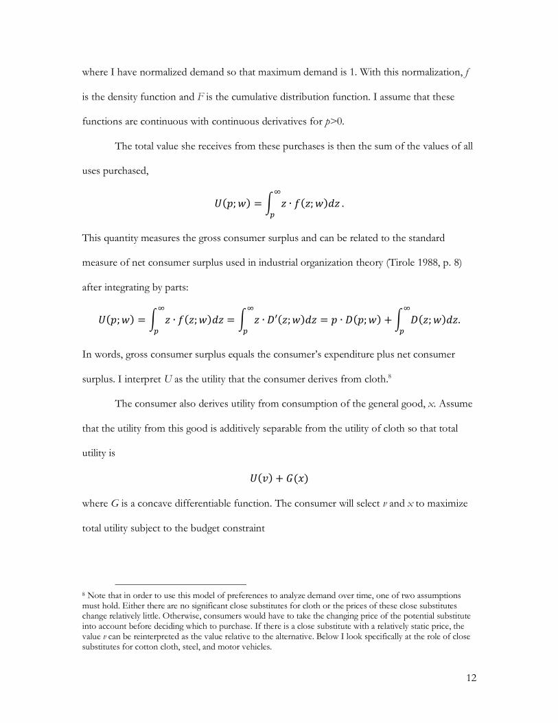
where I have normalized demand so that maximum demand is 1. With this normalization, f
is the density function and F is the cumulative distribution function. I assume that these
functions are continuous with continuous derivatives for p>0.
The total value she receives from these purchases is then the sum of the values of all
uses purchased,
𝑈(𝑝; 𝑤) = * 𝑧 ∙ 𝑓(𝑧; 𝑤)𝑑𝑧.
/.
This quantity measures the gross consumer surplus and can be related to the standard
measure of net consumer surplus used in industrial organization theory (Tirole 1988, p. 8)
after integrating by parts:
𝑈(𝑝;𝑤) = * 𝑧 ∙ 𝑓(𝑧;𝑤)𝑑𝑧.
/= * 𝑧 ∙ 𝐷′(𝑧;𝑤)𝑑𝑧
.
/= 𝑝 ∙ 𝐷(𝑝;𝑤) +* 𝐷(𝑧; 𝑤)𝑑𝑧.
.
/
In words, gross consumer surplus equals the consumer’s expenditure plus net consumer
surplus. I interpret U as the utility that the consumer derives from cloth.8
The consumer also derives utility from consumption of the general good, x. Assume
that the utility from this good is additively separable from the utility of cloth so that total
utility is
𝑈(𝑣) + 𝐺(𝑥)
where G is a concave differentiable function. The consumer will select v and x to maximize
total utility subject to the budget constraint
8 Note that in order to use this model of preferences to analyze demand over time, one of two assumptions must hold. Either there are no significant close substitutes for cloth or the prices of these close substitutes change relatively little. Otherwise, consumers would have to take the changing price of the potential substitute into account before deciding which to purchase. If there is a close substitute with a relatively static price, the value v can be reinterpreted as the value relative to the alternative. Below I look specifically at the role of close substitutes for cotton cloth, steel, and motor vehicles.

13
(1)
𝑤 ≥ 𝑥 + 𝑝𝐷(𝑣)
where the price of the general good is taken as numeraire and w is the consumer’s wage (all
consumers are workers). The consumer’s Lagrangean can be written
(2)
ℒ(𝑣, 𝑥) = 𝑈(𝑣) + 𝐺(𝑥) + 𝜆A𝑤 − 𝑥 − 𝑝 ∙ 𝐷(𝑣)B.
Taking the first order conditions,
(3)
𝐺C = 𝜆,𝑣D(𝑝,𝑤) = 𝑝𝜆 = 𝑝 ∙ 𝐺C(𝑥D(𝑝,𝑤))
where the subscript designates a derivative.
Production
Let there be three sectors, one producing cloth, one producing good x, and one
producing an investment good, quantity I. Each sector is composed of many firms in
competitive markets. The aggregate output of cloth, 𝑌 = 𝑌(𝐿, 𝐾, 𝑡), where L is textile labor,
K is capital, t captures technical change, and 𝑌(∙) is a constant returns production function
that is continuous and differentiable.9 Capital and the general good, x, are produced using
simpler production functions
𝑋 = 𝑎 ∙ 𝐿C,𝐼 = 𝑎 ∙ 𝐿L,𝑁 = 𝐿 + 𝐿C + 𝐿L
where X is the aggregate output of x, N is population (or workforce), 𝐿C and 𝐿L are the
workforce size in the x and I production sectors, and a is a measure of general productivity
that increases over time. Taking the price of good x and the investment good as numeraire,
aggregate profits of each sector are
9 Note that this production function is quite general and can accommodate labor-replacing technical change as in Acemoglu and Restrepo (2018) and Hemous and Olsen (2016).

14
(4)
𝜋O = 𝑝 ∙ 𝑌 − 𝑤 ∙ 𝐿 − 𝑟 ∙ 𝐾,𝜋C = 𝑋 − 𝑤 ∙ 𝐿C,𝜋L = 𝐼 − 𝑤 ∙ 𝐿L.
Firms in each sector employ a fraction of the aggregate labor and capital for that sector and
earn the same fraction of profits. The first order profit maximizing conditions imply
(5)
𝑤 = 𝑎 = 𝑝 ∙ 𝑌Q.
Assuming that competitive markets generate zero profits in each sector and equating
aggregate income (𝑤𝑁 + 𝑟𝐾) with aggregate output (𝑝𝑌 + 𝑋 + 𝐼), it is straightforward to
show that consumption expenditures per capita equal w, as in the individual budget
constraint, (1).
Finally, since I am concerned here just with the determinants of the demand for
cloth, I do not specify the savings function and the dynamic growth path of capital.
Equations (3) and (5) will hold at each point in time. Also, I assume that textile consumption
(or steel or autos) is very small compared to total consumption, 𝑝𝑌 ≪ 𝑋. The consumption
of cotton textiles, steel, and motor vehicles never exceeded a few percent of income during
the entire period studied. Note that this implies that SCDS/≈ 0 and 𝑋 ≈ 𝑤𝑁 so that each
individual’s consumption of x is 𝑥D ≈ 𝑤 .
Inverted-U in Employment
Technology and employment
It is useful to define labor productivity in cloth production, A, and labor share of
output, s,
15
(6)
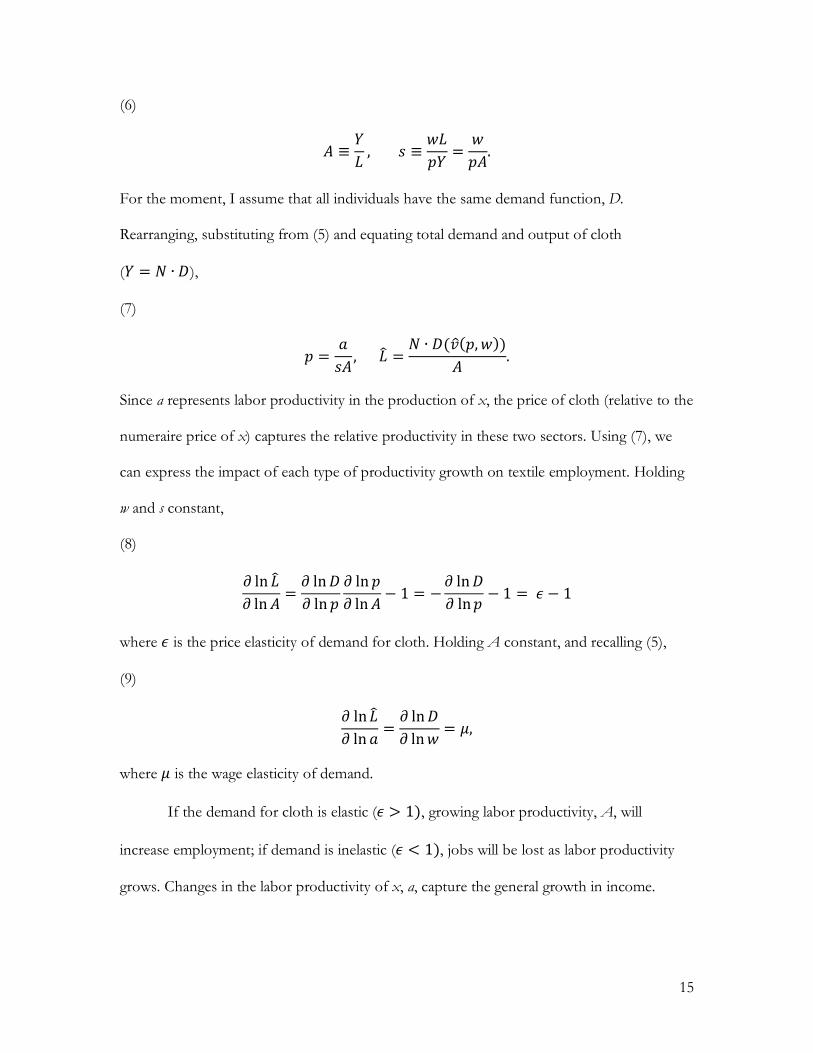
𝐴 ≡𝑌𝐿 ,𝑠 ≡
𝑤𝐿𝑝𝑌 =
𝑤𝑝𝐴.
For the moment, I assume that all individuals have the same demand function, D.
Rearranging, substituting from (5) and equating total demand and output of cloth
(𝑌 = 𝑁 ∙ 𝐷),
(7)
𝑝 =𝑎𝑠𝐴,𝐿
X =𝑁 ∙ 𝐷(𝑣D(𝑝, 𝑤))
𝐴 .
Since a represents labor productivity in the production of x, the price of cloth (relative to the
numeraire price of x) captures the relative productivity in these two sectors. Using (7), we
can express the impact of each type of productivity growth on textile employment. Holding
w and s constant,
(8)
𝜕 ln 𝐿X𝜕 ln𝐴 =
𝜕 ln𝐷𝜕 ln 𝑝
𝜕 ln 𝑝𝜕 ln𝐴 − 1 = −
𝜕 ln𝐷𝜕 ln𝑝 − 1 = 𝜖 − 1
where 𝜖 is the price elasticity of demand for cloth. Holding A constant, and recalling (5),
(9)
𝜕 ln𝐿X𝜕 ln 𝑎 =
𝜕 ln𝐷𝜕 ln𝑤 = 𝜇,
where 𝜇 is the wage elasticity of demand.
If the demand for cloth is elastic (𝜖 > 1), growing labor productivity, A, will
increase employment; if demand is inelastic (𝜖 < 1), jobs will be lost as labor productivity
grows. Changes in the labor productivity of x, a, capture the general growth in income.
16
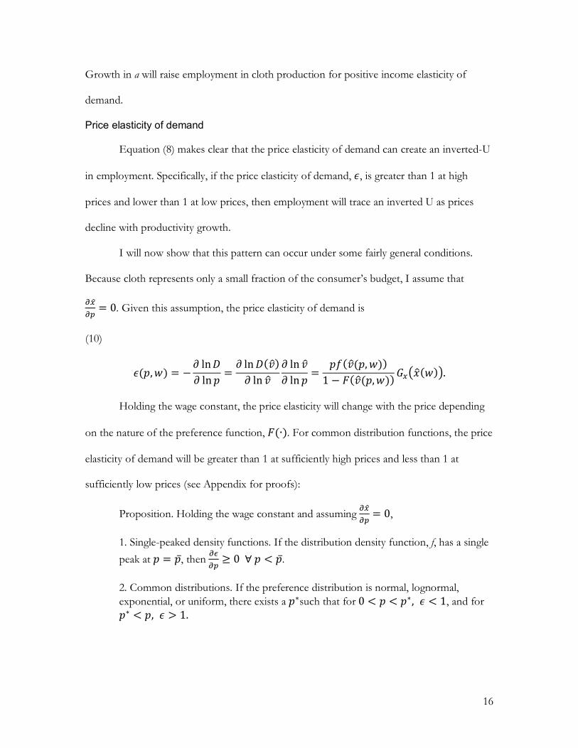
Growth in a will raise employment in cloth production for positive income elasticity of
demand.
Price elasticity of demand
Equation (8) makes clear that the price elasticity of demand can create an inverted-U
in employment. Specifically, if the price elasticity of demand, 𝜖, is greater than 1 at high
prices and lower than 1 at low prices, then employment will trace an inverted U as prices
decline with productivity growth.
I will now show that this pattern can occur under some fairly general conditions.
Because cloth represents only a small fraction of the consumer’s budget, I assume that
SCDS/= 0. Given this assumption, the price elasticity of demand is
(10)
𝜖(𝑝,𝑤) = −𝜕 ln𝐷𝜕 ln 𝑝 =
𝜕 ln𝐷(𝑣D)𝜕 ln 𝑣D
𝜕 ln 𝑣D𝜕 ln 𝑝 =
𝑝𝑓(𝑣D(𝑝, 𝑤))1 − 𝐹(𝑣D(𝑝,𝑤)) 𝐺C
A𝑥D(𝑤)B.
Holding the wage constant, the price elasticity will change with the price depending
on the nature of the preference function, 𝐹(∙). For common distribution functions, the price
elasticity of demand will be greater than 1 at sufficiently high prices and less than 1 at
sufficiently low prices (see Appendix for proofs):
Proposition. Holding the wage constant and assuming SCDS/= 0,
1. Single-peaked density functions. If the distribution density function, f, has a single peak at 𝑝 = �̅�, then S`
S/≥ 0∀𝑝 < �̅�.
2. Common distributions. If the preference distribution is normal, lognormal, exponential, or uniform, there exists a 𝑝∗such that for 0 < 𝑝 < 𝑝∗, 𝜖 < 1, and for 𝑝∗ < 𝑝, 𝜖 > 1.

17
These propositions suggest that the model of demand derived from distributions of
preferences can account for the inverted U curve in employment under fairly general
circumstances as long as price starts above 𝑝∗ and declines below it.
While changes in the price elasticity of demand drive the inverted-U shape in this
model, the income elasticity of demand also changes and the level of demand is influenced
by both changes in productivity and income more generally. In the empirical section of the
paper, I use a nonparametric analysis to show that both factors are important in determining
per capita demand and then I use parametric estimates to explore how well the model fits
the time series data.
Data
Time series over a century in length often require combining data from different
sources involving various adjustments. I describe the data sources and adjustments in detail
in the Appendix. This section describes the main data series used in estimating employment
in cotton textiles, steel, and automotive industries and in the computer technology analysis.
Production and demand
I use physical quantities to measure production and demand. For the textile industry,
I measure output as yards of cotton cloth produced plus yards of cloth made of synthetic
fibers from 1930 on. From 1958, I use the deflated output of the cotton and synthetic fiber
broadwoven cloth industries (SIC 2211 and 2221). For the early years, I also included
estimates of cotton cloth produced in households. For steel, I used the raw short tons of
steel produced. For the motor vehicle industry I used the number of passenger vehicles and
trucks produced each year.

18
To estimate per capita demand or consumption, I add net imports to the estimates
of domestic production and divide by the population.
Note that these measures do not adjust for product quality.10 This approach avoids
distortions that might arise from constructing quality adjusted price indices over long periods
of time. It does mean that “true” demand and productivity are understated. However, this
does not pose a significant problem for my analysis because I measure both without quality
adjustments. The distribution function I estimate would, of course, be different if it were
estimated with quality-adjusted data, but using unadjusted data allows for consistent
predictions of employment.
Employment, prices, and wages
I count the number of industry wage earners or, from 1958 on, the number of
production workers. For prices, I use the prices of standard commodities. For cotton
textiles, I use the wholesale price for cotton sheeting. For steel, I use wholesale prices for
steel rails. I do not have a similar commodity price for motor vehicles. The BLS does have a
price index for the automotive industry, but this measure implicitly changes as the quality of
vehicles improved. I need to use a commodity type price because my measures of output and
consumption (cars and trucks) does not capture these quality improvements. For wages, I
use the compensation of manufacturing production workers. This measure includes the
value of employee benefits from 1906 on.
Because price data are limited, I also obtain data on labor’s share of output, the wage
bill divided by the value of product shipped. Prices relative to wages can then be estimated
from labor share and labor productivity series because from (6), 𝑝 𝑤 = 𝑠 ∙ 𝐴⁄ .
10 The deflators used from 1958 on in cotton are quality adjusted but the series closely matches the unadjusted output measure during the years when they overlap.

19
Labor productivity
I calculate labor productivity by dividing output by the number of production
employees times the number of hours worked per year. I use industry specific estimates of
hours if available and estimates of hours for manufacturing workers if not.
Over the sample periods, each industry exhibited rapid labor productivity growth.
From 1820 to 1995, labor productivity in cotton textiles grew 2.9% per year; in steel, it grew
2.4% per year from 1860 to 1982; in motor vehicles, it grew 1.4% per year from 1910
through 2007. Figure 2 shows labor productivity for each industry on a log scale over time.
Each industry exhibits steady productivity growth over long periods of time. Textiles and
especially automotive show initially higher rates of growth; steel exhibits faster growth since
the 1970s, likely the effect of steel minimills that use recycled steel rather than blast furnace
production of iron.

20
Figure 2. Labor Productivity over Time

21
Empirical Findings
Are productivity and income both important for structural change?
As noted above, the literature on sectoral change largely divides into papers that see
deindustrialization arising from the relative productivity of the manufacturing sector and
other papers that see rising incomes as the driver instead. My model (and Boppart 2014) sees
both factors as important in explaining the rise and fall of employment in specific industries,
especially because productivity growth has been an order of magnitude larger than income
growth.
Table 1 explores the relative explanatory power of both factors non-parametrically,
specifically with quadratic forms similar to this:
ln𝐷 = 𝛼 + 𝛽f ln𝑤 + 𝛽g(ln𝑤)g + 𝛾f ln𝐴 + 𝛾g(ln𝐴)g + 𝜀.
I perform this regression using two different measures of income and labor productivity. F
tests on the null hypotheses that 𝛽f = 𝛽g = 0 and 𝛾f = 𝛾g = 0 provide one measure of
explanatory significance. The left hand panel uses real GDP per capita as the income
measure; the right panel uses the real production wage (deflated by the CPI).
The F tests strongly reject the null hypothesis of no effect for the productivity
measures in all cases. By contrast, the null hypothesis is rejected for income only in the
motor vehicle industry; it cannot be rejected in cotton and steel. The implication is that
models based on income alone cannot sufficiently account for the changes in per capita
demand over time in all markets; models need to incorporate both income and productivity,
but especially productivity.
I also show the variance of each quadratic form using the estimated coefficients
divided by the variance of the dependent variable. This provides a crude measure of the
22
variance “explained” by each factor, ignoring covariances. These ratios also show that
variations in income can only account for a relatively small portion of the total variation in
consumption per capita.
Parametric estimates
Applying the model
The model above provides a parsimonious explanation for the inverted U shape of
industry employment observed over time. But how well does this highly simplified model
actually predict the patterns observed? A close fit would provide some support for its
relevance. However, the model abstracts away from several considerations that might
undermine efforts to fit the model, considerations that I discuss in this section. In general, I
find that the model fits the data for employment and consumption rather well despite these
concerns, except during the most recent decades of the textile and steel industries.
One concern is that the model assumes no substantial interference from close
substitute products. That means that either there are no substitutes or that the productivity
growth in substitutes is sufficiently slow that the effect of substitution can be taken as
constant. Each industry did have substitutes, especially during the early years. However, it
seems that these substitutes were fairly static technologically and were quickly overtaken.
Cotton cloth competed with wool and linen. However, wool and linen were mainly
produced within the household (Zevin 1971) and did not directly compete in most markets.
In urban markets where they did compete, wool tended to be substantially more expensive
per pound and its price declined only slowly compared to cotton.11 During the early years of
the Bessemer steel process, steel rails were much more expensive than iron rails, but steel
11 For example, in Philadelphia in 1820, wool was $0.75 per pound while cotton sheeting was $0.15 (US Bureau of the Census 1975).
23
rails lasted much longer, making the higher price worth it for many uses. By 1883, the price
of steel rails fell below the price of iron rails, eliminating the production of this substitute
(Temin 1964 p. 222). And cars and trucks competed with horse drawn vehicles during the
early years. However, here, too, production of horse drawn vehicles collapsed very quickly.12
It is also possible that new technologies introduce new substitutes or find new uses
for commodities, changing the shape of the preference distribution function. Since the
1970s, steel may have faced greater competition from aluminum and other materials for use
in cars and cans (Tarr 1988 p. 177-8), perhaps contributing to the poorer fit of the model
then (see below).
Another concern is that the distribution of preferences changes over time, for
instance, as income inequality changes. Also, product quality changes over time, distorting
consumption measures that are not adjusted for quality. In addition, the model does not take
into account time patterns of consumption for consumer durables (auto) and investment
goods (some steel). In any case, despite all these potential problems, the model fits the data
reasonably well.
Parameterizing the model
In order to investigate the model empirically, it is helpful to provide a flexible
functional form for 𝐺C :
(11)
𝐺CA𝑥D(𝑝,𝑤)B = 𝑥Djkf,0 ≤ 𝛼 < 1. 13
Recalling that the partial equilibrium assumption implies that 𝑥D ≈ 𝑤, (3) and (6) yield
12 The production of carriages, buggies, and sulkies fell from 538 thousand in 1914 to 34 thousand in 1921; the production of farm wagons, horse-drawn trucks, and business vehicles fell from 534 thousand in 1914 to 67 thousand in 1921 (US Bureau of the Census 1975). 13 Making 𝐺(𝑥) = 𝑥j if 𝛼 > 0 or 𝐺(𝑥) = ln 𝑥 if 𝛼 = 0.
24
(12)
𝑣D(𝑝, 𝑤) ≈𝑝𝑤 ∙ 𝑤
j = 𝑠 ∙ 𝐴 ∙ 𝑤j.
The first expression presents 𝑣D as the product of the ratio of price to the wage—as is
commonly specified in indirect utility functions—and a pure income term. The second
expression presents 𝑣D as the product of labor productivity in textiles and an income term
(the labor share of output is approximately constant during most of the sample period).
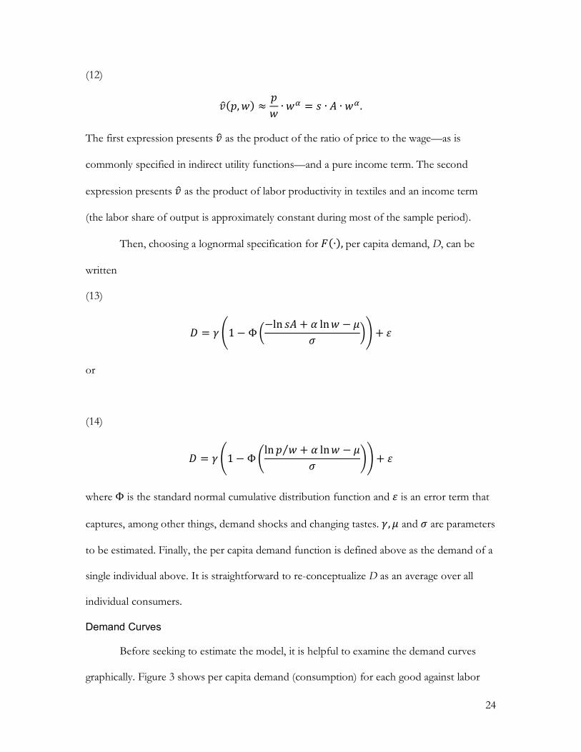
Then, choosing a lognormal specification for 𝐹(∙),per capita demand, D, can be
written
(13)
𝐷 = 𝛾 n1 − Φp−ln 𝑠𝐴 + 𝛼 ln𝑤 − 𝜇
𝜎 rs + 𝜀
or
(14)
𝐷 = 𝛾 n1 − Φtln 𝑝 𝑤⁄ + 𝛼 ln𝑤 − 𝜇
𝜎 us + 𝜀
where Φ is the standard normal cumulative distribution function and 𝜀 is an error term that
captures, among other things, demand shocks and changing tastes. 𝛾, 𝜇 and 𝜎 are parameters
to be estimated. Finally, the per capita demand function is defined above as the demand of a
single individual above. It is straightforward to re-conceptualize D as an average over all
individual consumers.
Demand Curves
Before seeking to estimate the model, it is helpful to examine the demand curves
graphically. Figure 3 shows per capita demand (consumption) for each good against labor

25
productivity times labor share of output, both on logarithmic scales. The solid line is simply
a log version of equation (13) fit to the data (with 𝛼 = 0 as discussed below).
Figure 3. Per Capita Consumption

26
In Figure 3A and 3B, the circles represent observations where the measure of
demand fails to capture the effect of imports of downstream products. Demand needs to

27
take trade into consideration and so I have calculated demand by adding net imports to the
amount of product produced domestically. However, for textiles and steel, further
adjustment is needed because these are intermediate goods industries. The ultimate
consumption good is produced by another industry and that good can be imported as well.
For example, the consumption of textiles in the form of apparel includes: 1) apparel
produced in the US with US cloth, 2) textiles that were imported to the US and used by
domestic apparel producers, and 3) apparel produced outside the US using cloth also
produced outside the US. Even after adjusting for imports of textiles, my measure of
consumption misses the cloth imported in apparel made abroad.
For this reason, I can only estimate demand for those years where downstream
imports are not too large. For textiles, I estimate demand through 1995; in 1996, imports
comprised a third of apparel imports for the first time and have grown rapidly since. For
steel, I estimate demand through 1982. After that, the largest steel-using industries,
fabricated metal products and machinery excluding computers (SIC 34 and 35 excluding
357), show a large increase in import penetration. Between 1982 and 1987, the import
penetration (net imports over domestic production) grew 10.5%. As the Figure shows, per
capita consumption falls dramatically around these cutoff years. Because the consumption
data become unrepresentative after these years, I estimate the model only for prior years. As
a robustness check, I used different cutoff years, but small changes in the cutoff year did not
change coefficient estimates significantly.
Model estimates
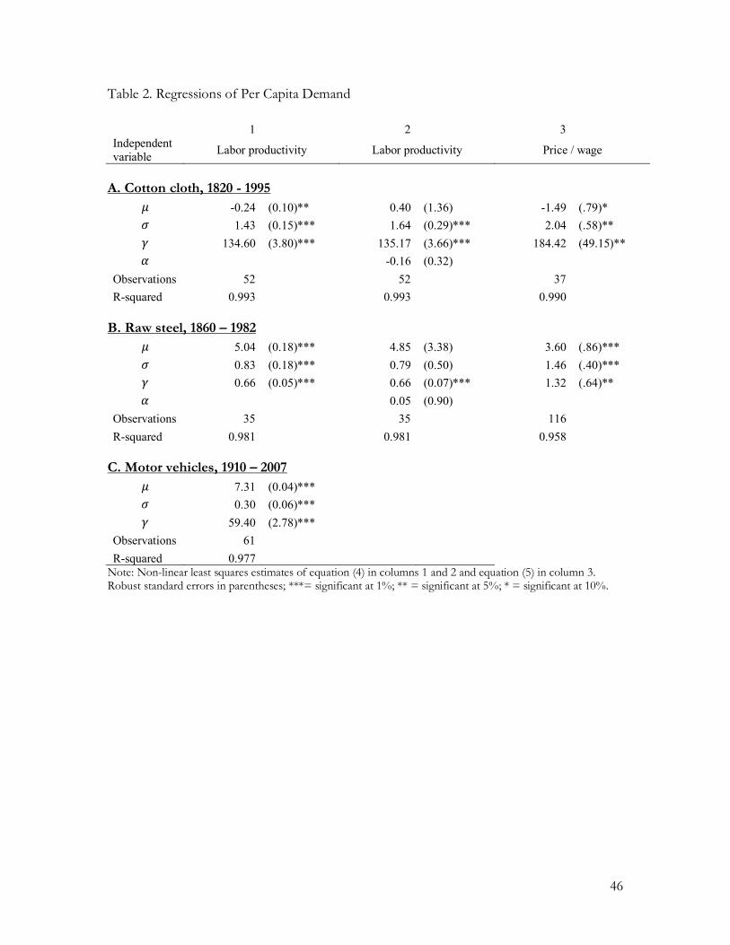
Table 2 shows NLLS estimates of equations (13) in columns 1 and 2 and estimates
of equation (14) for textile and steel in column 3. Columns 1 and 3 set 𝛼 = 0, excluding
secondary income effects. All of the regressions have a good fit, although the regressions
28
using labor productivity (columns 1 and 2) fit better than those using the ratio of prices to
wages (column 3), probably because of the greater volatility of wholesale price data. Note
that the model fits the data better than estimates using a simple quadratic form in Table 1.
None of the estimates in column 2 find a significant coefficient for 𝛼 and the NLLS
regression for the auto industry failed to converge for this specification. The lack of a
significant estimate of 𝛼 may be because of lack of statistical power, but it suggests that per
capita demand is close to a simple function of 𝑝 𝑤v . This specification corresponds to a
common assumption in the literature that indirect utility is a function of price over wage.
Recalling that w/= 𝑠𝐴, assuming that 𝛼 = 0 makes for a simple interpretation of
Figure 3. First, it is straightforward to show that with this assumption, the price elasticity of
demand equals the income elasticity of demand. Since the x-axes represent ln 𝑠𝐴 = lnw/
and
the vertical axes represent ln𝐷, the slope of the curve in each panel represents the elasticity
of demand (price and income). The shape of these curves neatly shows the decline in
elasticity accompanying the growth of productivity.
These predicted levels of per capita demand can also be used to estimate industry
production employment by dividing domestic demand (total demand divided by 1 + import
penetration) by the annual output per production worker. Measuring labor productivity as
output per production worker-hour this is14
𝐷𝑒𝑚𝑎𝑛𝑑𝑝𝑒𝑟𝑐𝑎𝑝𝑖𝑡𝑎 ∙ 𝑃𝑜𝑝𝑢𝑙𝑎𝑡𝑖𝑜𝑛1 + 𝐼𝑚𝑝𝑜𝑟𝑡𝑝𝑒𝑛𝑒𝑡𝑟𝑎𝑡𝑖𝑜𝑛 ∙
1𝐿𝑎𝑏𝑜𝑟𝑝𝑟𝑜𝑑𝑢𝑐𝑡𝑖𝑣𝑖𝑡𝑦 ∙ 𝐻𝑜𝑢𝑟𝑠𝑤𝑜𝑟𝑘𝑒𝑑/𝑦𝑒𝑎𝑟.
These estimates are shown as the solid lines in Figure 1. The estimates appear to be
accurate over long periods of time. There are notable drops in employment during the Great
14 For 1820 and before, I also subtract the estimate of labor performed in households.

29
Depression and excess employment in motor vehicles during World War II. Finally,
employment drops sharply for the years when my measure of consumption fails in textiles
(after 1995) and steel (after 1982). It appears that this simple model using a lognormal
distribution of preferences provides a succinct explanation of the inverted U in employment
in these industries.
Implications
The Industrial Revolution
Robert Zevin (1971) describes the “remarkable explosion” of economic activity at
the beginning of the nineteenth century that was dominated by the cotton textile industry:
The first great expansion of modern industrial activity in the United States took place in New England from the end of the War of 1812 to the middle of the 1830s. By the census of 1840 factories had become familiar landmarks at hundreds of New England waterpower sites; large cities such as Lowell and Holyoke had been created entirely by the advance of industrial activity, while Fall River, Pawtucket, Worcester, and the like had been greatly enlarged and transformed by the same advance. About 100,000 people were employed by large-scale manufacturing enterprises, with 20 or 30 employing up to 1500 employees each (pp. 122-3).
In Zevin’s interpretation, this change was mostly driven by rapid demand growth,
reaching peak rates of 8 or 9 percent per year. He cites the growing population of the West
as the principle cause, with growing incomes, urbanization, the high price of substitutes, and
lower transportation costs also contributing. Zevin additionally notes that the price elasticity
of demand declined, although he does not offer an explanation as to why this happened.
My estimates do not contradict Zevin’s analysis—he guesses that the price elasticity
of demand began at around 2.5, similar to my estimate. But my analysis puts the growth rate
of employment into a longer-term context. The growth of the West was surely important,
especially before 1820 when it was particularly rapid. Yet the initial high elasticity of demand
30
and its subsequent decline generate a rising and then ebbing tide of labor growth in an
industry where labor productivity has persistently grown at 3 percent per year.
My analysis suggests that this pattern—high initial demand elasticity that declines
over time—might be more general, contributing to high initial employment growth in the
steel and auto industries as well as, perhaps, in other leading industries. That is, the
“remarkable explosion” in industrial activity in textiles and in other leading industries may
have derived from a potent combination of high productivity growth and highly elastic
demand. And the decline in demand elasticity reconciles the high employment growth of the
past with the current job losses in many manufacturing industries. Of course, not all
industries exhibited these characteristics; the “leading industries” were precisely those
industries characterized by rapid growth.
It has long been recognized that industrial development was uneven, that new
technology altered some industries but not others. The analysis here suggests that differences
in demand might also have been important in shaping the pattern of development. For
example, the high elasticity of demand for some manufacturing industries might help explain
the transition from workshop to factory even in non-mechanized industries. Sokoloff (1984)
presents evidence of such a transformation from 1820 to 1850, arguing that even without
mechanization, many factories achieved productivity gains through a finer division of labor.
It seems likely that these establishments realized productivity gains, but gains of a smaller
magnitude than some of the mechanized factories. Yet many of these firms may have been
in industries with high demand elasticity so that they experienced significant growth in
demand even though their productivity gains might have been relatively modest.
The early elasticity of demand also helps explain why technological change during
the early nineteenth century has been described as an Industrial Revolution. Abramovitz and

31
David (2001) estimated that overall output per manhour in the US grew at only 0.39 percent
per year from 1800 through 1855. Yet this slow rate of growth was accompanied by leading
industries where demand was growing 8 or 9 percent annually. Society was transformed
despite the slow overall rate of growth.
In general, because new technologies were addressing markets with large unmet
needs—the upper tail of the consumer preference distribution—the price and income
elasticities of demand were high and this tended to accelerate other processes. For example,
the emergence of national product markets surely had much to do with the decline in
transportation costs (much of it driven by new technology) and the growing Western
population. But the high elasticity of demand for many manufactured products would have
increased the payoffs to market expansion, accelerating the rise of national markets.
Similarly, the slowing of demand growth as markets matured may have heightened market
competition, hastening the merger and trust movement of the late nineteenth century.
Trade vs. technology in manufacturing job losses
The model provides an estimate of the impact of technology on industry
employment as mediated by demand. We can use this to understand how much technology
contributed to the loss of manufacturing jobs compared to other factors including trade.
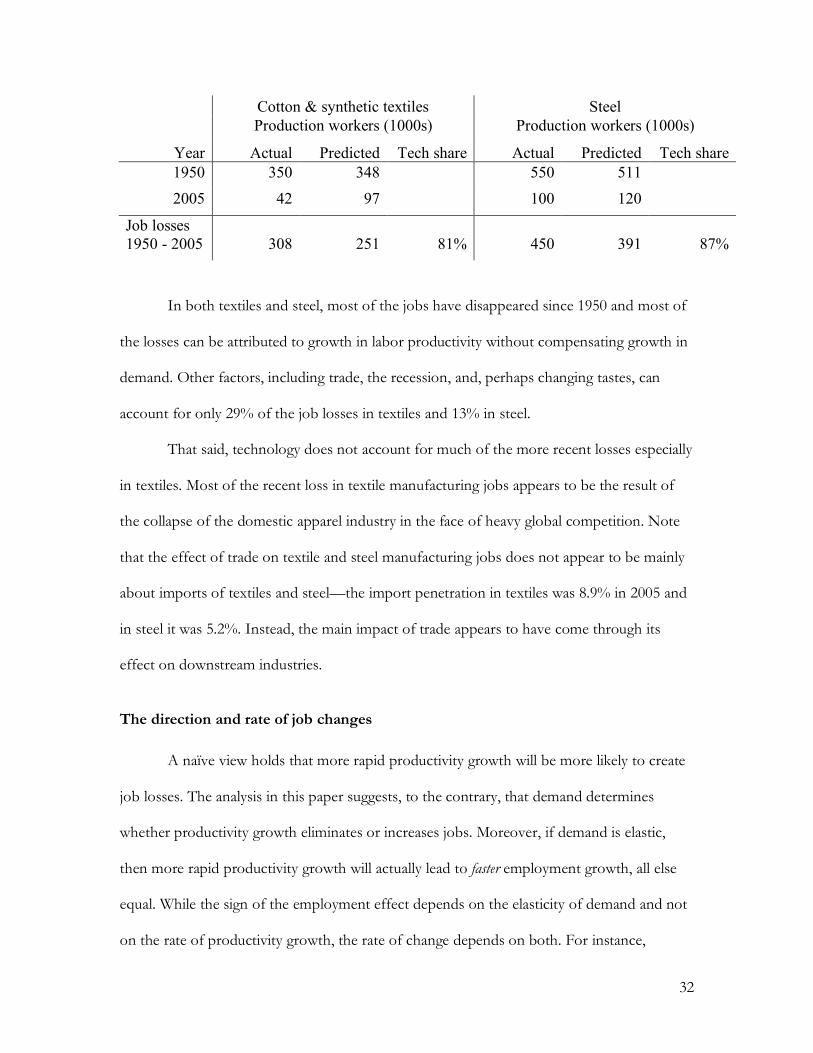
Using predicted industry employment without the correction for imports, actual and
predicted employment changes can be compared:
32
Cotton & synthetic textiles Steel
Production workers (1000s) Production workers (1000s)
Year Actual Predicted Tech share Actual Predicted Tech share 1950 350 348
550 511
2005 42 97
100 120
Job losses 1950 - 2005 308 251 81% 450 391 87%
In both textiles and steel, most of the jobs have disappeared since 1950 and most of
the losses can be attributed to growth in labor productivity without compensating growth in
demand. Other factors, including trade, the recession, and, perhaps changing tastes, can
account for only 29% of the job losses in textiles and 13% in steel.
That said, technology does not account for much of the more recent losses especially
in textiles. Most of the recent loss in textile manufacturing jobs appears to be the result of
the collapse of the domestic apparel industry in the face of heavy global competition. Note
that the effect of trade on textile and steel manufacturing jobs does not appear to be mainly
about imports of textiles and steel—the import penetration in textiles was 8.9% in 2005 and
in steel it was 5.2%. Instead, the main impact of trade appears to have come through its
effect on downstream industries.
The direction and rate of job changes
A naïve view holds that more rapid productivity growth will be more likely to create
job losses. The analysis in this paper suggests, to the contrary, that demand determines
whether productivity growth eliminates or increases jobs. Moreover, if demand is elastic,
then more rapid productivity growth will actually lead to faster employment growth, all else
equal. While the sign of the employment effect depends on the elasticity of demand and not
on the rate of productivity growth, the rate of change depends on both. For instance,

33
although productivity grew faster in cotton textiles than in auto (after 1914), employment
grew faster in auto; the distribution of preferences for motor vehicles was much more
concentrated (small 𝜎) than the distribution for textiles.
One might expect that computer technology would have a different effect on job
growth across industries depending on industry demand elasticity. Assuming that the
historical process of deindustrialization means that manufacturing industries have less elastic
(more satiated) demand than most other industries on average, then computer technology
should have a relatively more negative impact on employment in manufacturing industries,
all else equal.15
Several recent papers find that information technology increases employment for
some groups and does not appear to reduce net employment, except in manufacturing.
Gaggl and Wright (2014) find that ICT tended to raise employment in wholesale, retail, and
finance industries, but had no statistically significant effect on other sectors, including
manufacturing. Akerman, Gaarder, and Mogstad (2015) find that Internet technology
increased employment of skilled workers and had no effect on unskilled. Mann and
Püttmann (2017) find that automation increases jobs in services but decreases them in
manufacturing. Bessen (2016) finds that computers tend to increase occupational
employment modestly overall, with job losses in low wage occupations. Autor, Dorn, and
Hansen (2015) find that local markets susceptible to computerization are not more likely to
experience employment loss. Autor and Salomons (2018) find that productivity growth is
15 To the extent that information technology allows manufacturers to create new products, then the technology might tap into new sources of demand and thus be more elastic. There is some evidence that information technology is used to create new products (see for example Bartel, Ichniowski, and Shaw 2007). New product varieties might provide a reason that the association between IT and employment growth in manufacturing is only weakly negative.

34
associated with net increases in employment, although direct effects in some industries are
negative.
Conclusion
A simple model explains the rise and subsequent fall of manufacturing employment
in the face of ongoing productivity growth. Productivity-enhancing technology will increase
industry employment if product demand is sufficiently elastic. Technical change reduces the
labor required needed to produce a unit of output, but it also reduces prices in competitive
markets. If the price elasticity of demand is greater than one, the increase in demand will
more than offset the labor-saving effect of the technology.
Understanding the responsiveness of demand is thus key to understanding whether
major new technologies will decrease or increase employment in affected industries. This
paper proposes that industry employment dynamics can be analyzed by deriving demand
from a distribution of preferences. For many distribution functions, the elasticity of demand
declines as price declines and productivity grows. In particular, a parsimonious model using a
lognormal distribution fits the demand curves well for cotton textiles, steel, and motor
vehicles over long periods of time.
This model generates an industry life cycle explanation for the inverted U pattern of
industrialization/deindustrialization seen in manufacturing employment. At high initial
prices, industries have large unmet demand that is highly elastic. Productivity improvements
give rise to robust job growth. Over time and with ongoing productivity gains, prices
progressively decline until most demand is met and the price elasticity of demand is quite
low. Then further productivity gains bring reduced employment.

35
This model thus reconciles the role of technological change in deindustrialization
today with its role spurring employment growth in the past. Demand plays a major role in
understanding the pattern of change in the Industrial Revolution and subsequent
technological revolutions.
This view implies that major new technologies today should increase employment if
they improve productivity in markets that have large unmet needs. Some evidence suggests
that this is the case with information technology and other recent forms of automation. This
model challenges a popular view that faster technical change is more likely to eliminate jobs.
Some people argue that because of Moore’s Law, the rate of change will be fast in new
information technologies and this will cause unemployment (Ford 2015). However, if
demand is elastic, faster technical change will, instead, create faster employment growth.
Faster technical change will, however, also hasten the day when demand is no longer so
elastic and deindustrialization sets in.
This analysis raises a number of other questions. For one, it would be helpful to
understand what factors shape the preference distribution functions. For instance, in the
model, the pace of industrialization/deindustrialization is affected by the variance of the
distribution of preferences. Nations with greater income equality might have more
homogenous preferences and hence a narrower distribution (smaller standard deviation). A
narrower distribution of preferences, in turn, implies more rapid employment growth during
industrialization. In this way, income inequality might slow the pace of economic
development. Correspondingly, income inequality might also affect the pace of
deindustrialization as markets mature. Another area for investigation concerns trade. The
model in this paper abstracts away from the effect of imports on demand. Clearly, imports

36
might play a role in decelerating industrial development in exposed economies, heightening
patterns of “premature deindustrialization” (Rodrik 2017).

37
Appendix
Propositions
To simplify notation, let 𝐺C = 1. Then, keeping wages constant,
𝜖(𝑝) =𝑝𝑓(𝑝)1 − 𝐹(𝑝)
so that
𝜕𝜖(𝑝)𝜕𝑝 =
𝑓�𝑝1 − 𝐹 +
𝑓g𝑝(1 − 𝐹)g +
𝑓1 − 𝐹 = 𝜖 t
𝑓′𝑓 +
𝑓1 − 𝐹 +
1𝑝u
Note that the second and third terms in parentheses are positive for 𝑝 > 0; the first term
could be positive or negative. A sufficient condition for S`S/≥ 0 is
(A1)
𝑓′𝑓 +
𝑓1 − 𝐹 ≥ 0.
Proposition 1. For a single peaked distribution with mode �̅�, for 𝑝 < �̅� , 𝑓� ≥ 0 so that
S`S/≥ 0.
Proposition 2. For each distribution, I will show that
𝜕𝜖𝜕𝑝 ≥ 0, lim
/→6𝜖 = 0, lim
/→.𝜖 = ∞.
Taken together, these conditions imply that for sufficiently high price, 𝜖 > 1, and for a
sufficiently low price, 𝜖 < 1.
a. Normal distribution
𝑓(𝑝) =1𝜎 𝜑
(𝑥),𝐹(𝑝) = Φ(𝑥),𝜖(𝑝) =𝑝𝜎
𝜑(𝑥)(1 − Φ(𝑥)) ,𝑥 ≡
𝑝 − 𝜇𝜎

38
where 𝜑 and Φ are the standard normal density and cumulative distribution functions
respectively. Taking the derivative of the density function,
𝑓�
𝑓 +𝑓
1 − 𝐹 = −𝑥𝜎 +
𝜑(𝑥)𝜎A1 − Φ(𝑥)B
.
A well-known inequality for the normal Mills’ ratio (Gordon 1941) holds that for x>0,16
(A2)
𝑥 ≤𝜑(𝑥)
1 − Φ(𝑥).
Applying this inequality, it is straightforward to show that (A1) holds for the normal
distribution. This also implies that lim/→.
𝜖 = ∞. By inspection, 𝜖(0) = 0.
b. Exponential distribution
𝑓(𝑝) ≡ 𝜆𝑒k�/,𝐹(𝑝) ≡ 1 − 𝑒k�/,𝜖(𝑝) = 𝜆𝑝,𝜆, 𝑝 > 0.
Then
𝑓�
𝑓 +𝑓
1 − 𝐹 = −𝜆 + 𝜆 = 0
so (A1) holds. By inspection, 𝜖(0) = 0 and lim/→.
𝜖 = ∞.
c. Uniform distribution
𝑓(𝑝) ≡1𝑏 ,𝐹
(𝑝) ≡𝑝𝑏 ,𝜖
(𝑝) =𝑝
𝑏 − 𝑝 ,0 < 𝑝 < 𝑏
so that
𝑓�
𝑓 +𝑓
1 − 𝐹 =1
𝑏 − 𝑝 > 0.
By inspection, 𝜖(0) = 0 and lim/→�
𝜖 = ∞.
16 I present the inverse of Gordon’s inequality.

39
d. Lognormal distribution
𝑓(𝑝) ≡1𝑝𝜎 𝜑
(𝑥),𝐹(𝑝) ≡ Φ(𝑥),𝜖(𝑝) =1𝜎
𝜑(𝑥)A1 − Φ(𝑥)B
,𝑥 ≡ln 𝑝 − 𝜇
𝜎
so that
𝜕𝜖(𝑝)𝜕𝑝 = 𝜖 t
𝑓′𝑓 +
𝑓1 − 𝐹 +
1𝑝u = 𝜖 p−
1𝑝 −
𝑥𝑝𝜎 +
𝜑𝑝𝜎(1 −Φ) +
1𝑝r.
Cancelling terms and using Gordon’s inequality, this is positive. And taking the limit of
Gordon’s inequality, lim/→.
𝜖 = ∞. By inspection lim/→6
𝜖 = 0.
Historical data sources
I obtain data on production employees for cotton and steel from Lebergott (1966, see also US Bureau of the Census 1975) through 1950, and from 1958 on from the NBER-CES manufacturing database for SIC 2211 and 2221 (broadwoven fabric mills, cotton and manmade fibers and silk) and SIC 3312 (primary iron and steel). The former measures the number of wage earners while the more recent series measure production employees. I find that these series are reasonably close for overlapping years. For 1820 in cotton, I estimate 5,600 full time equivalent workers producing in households, using estimates of household production and Davis and Stettler’s (1966) estimates of output per worker. For the auto industry, I use the BLS Current Employment Statistics series for motor vehicle production workers from 1929 on. For 1910 and 1920, I obtained the number of employees in the motor vehicle industry from the 1% Census samples (Ruggles et al. 2015) and prorated those figures by the ratio of BLS production workers to Census industry employees for 1930.
Weekly hours data for motor vehicles also come from the BLS from 1929 on. For earlier years and for cotton and steel before 1958, I use Whaples (2001) before 1939, linearly interpolating for missing year observations. From 1939 to 1958 I use the BLS Current Employment Statistics series for manufacturing production and nonsupervisory personnel. In cotton and steel, I use the NBER-CES data for production hours from 1958 on (this comes from the BLS industry data).
For cotton production, I begin with Davis and Stettler’s (1966, Table 9) estimates of yards produced per man-year for 1820 and 1831 multiplied by the estimate of the number of cotton textile wage earners for those years (I assume productivity was the same in 1830 and 1831). For 1820, I estimate that an additional 9.6 million yards were produced in households based on data from Tryon (1917). From 1830 on, Tryon’s estimates indicate little cotton cloth was produced at home. From 1840 through 1950, I use estimates of the pounds of cotton consumed in textile production times three yards per pound (US Bureau of the Census 1975 and Statistical Abstracts, various years). This ratio is the historically used rule of thumb, but I also found that it applies reasonably well to a variety of twentieth century test statistics. While some cotton is lost in the production process (5% or less typically), these losses changed little over time. From 1930 on, I also include the weight of manmade fibers
40
consumed in textile production. From 1958 on I found that the deflated output of SIC 2211 and 2221 in the NBER-CES tracked the pounds of fiber consumed closely for the ten years when I had measures of both. I used the average ratio for these years to estimate yards of cloth produced based on the NBER-CES real output from 1958 on. For steel, my output measure is the short tons of raw steel produced (Carter 2006). From 1913 through 1950, I measure motor vehicle production using the NBER Macrohistory Database series on passenger car and truck production. I obtained a figure for 1910 production from Wikipedia.17 From 1951 on, I use car and truck production figures from the Ward’s Automotive Yearbook, prorated to match the NBER series.
For consumption of motor vehicles, I use the Ward’s Automotive series on sales of passenger cars and trucks. For cotton and steel, I add net imports to domestic production. For cotton from 1820 through 1950, I use the net dollar imports of cotton manufactures divided by the price of cloth. From 1820 through 1860, I use Sandberg’s (1971) estimate of the price of British imports; from 1860 through 1950, I use the price of cotton sheeting (see below). From 1958 on, I use import penetration ratios from Feenstra (1958 though 1994) and Schott (1995 on). For steel, I use Temin’s (1964, p. 282) estimates for steel rail imports from 1860 through 1889. I use the Feenstra and Schott import penetration estimates from 1958 on; I ignore steel imports between 1890 and 1957.
For prices, I use the series on cotton sheeting from 1820 through 1974 (Carter 2006, Cc205); for steel I use series for the price of steel rails, splicing together separate series for Bessemer, open hearth, standard, and carbon steel (Carter 2006, CC244-7).
References
Abramovitz, Moses and Paul David. “Two Centuries of American Macroeconomic Growth: From Exploitation of Resource Abundance to Knowledge-Driven Development” SIEPR Discussion Paper No. 01-05 (2001).
Acemoglu, Daron, and Veronica Guerrieri. "Capital deepening and nonbalanced economic growth." Journal of political Economy 116.3 (2008): 467-498.
Acemoglu, Daron and Pascual Restrepo. 2018. “The Race Between Machine and Man: Implications of Technology for Growth, Factor Shares and Employment.” American Economic Review, forthcoming.
Akerman, Anders, Ingvil Gaarder, and Magne Mogstad. “The skill complementarity of broadband internet.” The Quarterly Journal of Economics (2015), 1781–1824.
Autor, David H. "Why are there still so many jobs? The history and future of workplace automation." The Journal of Economic Perspectives 29.3 (2015): 3-30.
Autor, David, David Dorn, and Gordon H. Hanson. "Untangling trade and technology: Evidence from local labour markets." Economic Journal 125.584 (2015): 621-46.
17 https://en.wikipedia.org/wiki/U.S._Automobile_Production_Figures.

41
Autor, David, and Anna Salomons, “Is automation labor-displacing? Productivity growth, employment, and the labor share,” Brookings Papers on Economic Activity, 2018 forthcoming.
Banks, James, Richard Blundell, and Arthur Lewbel. "Quadratic Engel curves and consumer demand." Review of Economics and statistics 79, no. 4 (1997): 527-539.
Bartel, Ann, Casey Ichniowski, and Kathryn Shaw. "How does information technology affect productivity? Plant-level comparisons of product innovation, process improvement, and worker skills." The Quarterly Journal of Economics 122.4 (2007): 1721-1758.
Baumol, William J. "Macroeconomics of unbalanced growth: the anatomy of urban crisis." The American economic review (1967): 415-426.
Becker, Randy, Wayne Gray, and Jordan Marvakov. NBER-CES Manufacturing Industry Database, 2016, http://www.nber.org/data/nberces.html
Bessen, James E. "How computer automation affects occupations: Technology, jobs, and skills." (2016).
Boppart, Timo. "Structural Change And The Kaldor Facts In A Growth Model With Relative Price Effects And Non-Gorman Preferences." Econometrica (2014): 2167-2196.
Buera, Francisco J., and Joseph P. Kaboski. "Can traditional theories of structural change fit the data?." Journal of the European Economic Association 7.2‐3 (2009): 469-477.
Carter, Susan B. Historical statistics of the United States: Earliest times to the present. Cambridge University Press, 2006.
Clark, Colin, The Conditions of Economic Progress. (1840) London: Macmillan.
Comin, Diego A., Danial Lashkari, and Martí Mestieri. Structural change with long-run income and price effects. No. w21595. National Bureau of Economic Research, 2015.
Davis, Lance E., and H. Louis Stettler III. "The New England Textile Industry, 1825–60: Trends and Fluctuations." In Dorothy Brady, ed., Output, employment, and productivity in the United States after 1800. NBER, 1966. 213-242.
Dennis, Benjamin N., and Talan B. İşcan. "Engel versus Baumol: Accounting for structural change using two centuries of US data." Explorations in Economic history 46.2 (2009): 186-202.
Diebolt, Claude. "La théorie de la sous-consommation du cycle des affaires de Emil Lederer", Economie Appliquée. An International Journal of Economic Analysis, Vol. 50, No. 1, 1997, pp. 27-50.

42
Dupuit, Jules. “De la mesure de l’utilité des travaux publics” 1844, Annales des ponts et chaussées, v.8 (2 sem), p.332-75
Engel, Ernst (1857). "Die Productions- und Consumtionsverhältnisse des Königreichs Sachsen". Zeitschrift des statistischen Bureaus des Königlich Sächsischen Ministerium des Inneren. 8–9: 28–29.
Feenstra, Robert, “U.S. Imports and Exports by 4-digit SIC Industry, 1958-94,” http://cid.econ.ucdavis.edu/usixd/usixd4sic.html.
Foellmi, Reto, and Josef Zweimüller. "Structural change, Engel's consumption cycles and Kaldor's facts of economic growth." Journal of monetary Economics 55.7 (2008): 1317-1328.
Gaggl, Paul, and Greg C. Wright. "A Short-Run View of What Computers Do: Evidence from a UK Tax Incentive." Working Paper (2014).
Gordon, Robert D. "Values of Mills' ratio of area to bounding ordinate and of the normal probability integral for large values of the argument." The Annals of Mathematical Statistics 12.3 (1941): 364-366.
Hémous, David, and Morten Olsen. "The rise of the machines: Automation, horizontal innovation and income inequality." (2016).
Jensen, J. Bradford, and Lori G. Kletzer. "Measuring tradable services and the task content of offshorable services jobs." Labor in the new economy. University of Chicago Press, 2010. 309-335.
Kollmeyer, Christopher. "Explaining Deindustrialization: How Affluence, Productivity Growth, and Globalization Diminish Manufacturing Employment 1." American Journal of Sociology 114.6 (2009): 1644-1674.
Kongsamut, Piyabha, Sergio Rebelo, and Danyang Xie. "Beyond balanced growth." The Review of Economic Studies 68.4 (2001): 869-882.
Lawrence, Robert Z., and Lawrence Edwards. "US employment deindustrialization: insights from history and the international experience." Policy Brief 13-27 (2013).
Lebergott, Stanley. "Labor Force and Employment 1800-1960." In Dorothy Brady, ed., Output, Employment and Productivity in the United States After 1800. National Bureau of Econonic Research, Studies in Income and Wealth 30 (1966).
Lewis, W. Arthur. "Economic development with unlimited supplies of labour." The manchester school 22.2 (1954): 139-191.
Mann, Katja and Lukas Püttmann, “Benign Effects of Automation: New Evidence From Patent Texts” working paper, 2017.
Matsuyama, Kiminori. "Agricultural productivity, comparative advantage, and economic growth." Journal of economic theory 58.2 (1992): 317-334.
43
Matsuyama, Kiminori. "Structural change in an interdependent world: A global view of manufacturing decline." Journal of the European Economic Association 7.2‐3 (2009): 478-486.
Matsuyama, Kiminori. "The rise of mass consumption societies." Journal of political Economy 110.5 (2002): 1035-1070.
NBER Macrohistory Database, Chapter 1, Production of Commodities. http://www.nber.org/databases/macrohistory/contents/chapter01.html.
Ngai, L. Rachel, and Christopher A. Pissarides. "Structural change in a multisector model of growth." The American Economic Review 97.1 (2007): 429-443.
Nickell, Stephen, Stephen Redding, and Joanna Swaffield. "The uneven pace of deindustrialisation in the OECD." The World Economy 31.9 (2008): 1154-1184.
Parker, William N., and Judith LV Klein. "Productivity growth in grain production in the United States, 1840–60 and 1900–10." Output, employment, and productivity in the United States after 1800. NBER, 1966. 523-582.
Rodrik, Dani. "Premature deindustrialization." Journal of Economic Growth 21.1 (2016): 1-33.
Rowthorn, Robert, and Ramana Ramaswamy. "Growth, trade, and deindustrialization." IMF Staff papers 46.1 (1999): 18-41.
Ruggles, Steven, Katie Genadek, Ronald Goeken, Josiah Grover, and Matthew Sobek. Integrated Public Use Microdata Series: Version 6.0 [Machine-readable database]. Minneapolis: University of Minnesota, 2015.
Sandberg, Lars. “A Note on British Cotton Cloth Exports to the United States: 1815-1860,” Explorations in Economic History, 9 (1971): 427-428.
Schott, Peter K. “U.S. Manufacturing Exports and Imports by SIC or NAICS Category and Partner Country, 1972 to 2005,” http://faculty.som.yale.edu/peterschott/sub_international.htm.
Sokoloff, Kenneth L. "Was the transition from the artisanal shop to the nonmechanized factory associated with gains in efficiency?: Evidence from the US Manufacturing censuses of 1820 and 1850." Explorations in Economic History 21, no. 4 (1984): 351-382.
Tarr, David G. “The steel crisis in the United States and the European Community: Causes and adjustments,” in Robert E. Baldwin, Carl B. Hamilton and Andre Sapir, editors, Issues in US-EC trade relations. University of Chicago Press, 1988. 173-200.
Temin, Peter. "Iron and Steel in 19th century America." An Economic Inquiry (1964). Massachusetts: MIT Press.

44
Tirole, Jean. The theory of industrial organization. MIT press, 1988.
Tryon, Rolla Milton. "Household manufactures in the United States, 1640-1860." (1917).
United States. Bureau of the Census. Historical Statistics Of The United States, Colonial Times To 1970. No. 93. US Department of Commerce, Bureau of the Census, 1975.
United States. Bureau of the Census. Statistical Abstract of The United States, various years.
United States. Department of Labor. Dictionary of Occupational Titles, Fourth edition, 1977.
Ward’s Automotive Yearbook, various years, Detroit: WardsAuto.
Whaples, Robert. “Hours of Work in U.S. History”. EH.Net Encyclopedia, edited by Robert Whaples. August 14, 2001. URL http://eh.net/encyclopedia/hours-of-work-in-u-s-history/
Zevin, Robert Brooke. "The growth of cotton textile production after 1815." Robert Fogel and Stanley Engerman, Reinterpretation of American Economic History, New York: Harper and Row (1971).

45
Tables
Table 1. Nonparametric tests of income and productivity Dependent variable: log consumption / capita
Income = GDP / capita Income = production wage
Quadratics in: Degrees freedom F
Prob. value
Share variance
Degrees freedom F
Prob. value
Share variance
Cotton Income 47 3.00 0.060 16% 47 0.20 0.818 1%
Productivity 47 150.16 0.000** 64% 47 23.27 0.000** 117% R-squared 0.981
0.980
Steel Income 30 0.72 0.497 3% 30 1.40 0.262 3%
Productivity 30 12.19 0.000** 70% 30 50.38 0.000** 120% R-squared 0.977
0.977
Autos Income 56 10.00 0.000** 15% 56 7.42 0.001** 14%
Productivity 56 185.00 0.000** 46% 56 25.82 0.000** 55% R-squared 0.933
0.916
Note: Each regression on ln consumption per capita includes two quadratic forms, one on the log of an income variable and one on the log of labor productivity. The reported F statistics are for tests of the null hypothesis that all of the quadratic coefficients are zero. The tests have 5 constraints and the residual degrees of freedom listed. **= significant at 1%; * = significant at 5%. The share of variance is the variance of the quadratic form over the variance of the dependent variable.
46
Table 2. Regressions of Per Capita Demand
1
2
3
Independent variable Labor productivity Labor productivity Price / wage
A. Cotton cloth, 1820 - 1995
𝜇 -0.24 (0.10)** 0.40 (1.36) -1.49 (.79)* 𝜎 1.43 (0.15)*** 1.64 (0.29)*** 2.04 (.58)** 𝛾 134.60 (3.80)*** 135.17 (3.66)*** 184.42 (49.15)** 𝛼
-0.16 (0.32)
Observations 52
52
37 R-squared 0.993
0.993
0.990
B. Raw steel, 1860 – 1982
𝜇 5.04 (0.18)*** 4.85 (3.38) 3.60 (.86)*** 𝜎 0.83 (0.18)*** 0.79 (0.50) 1.46 (.40)*** 𝛾 0.66 (0.05)*** 0.66 (0.07)*** 1.32 (.64)** 𝛼
0.05 (0.90)
Observations 35
35
116 R-squared 0.981
0.981
0.958
C. Motor vehicles, 1910 – 2007
𝜇 7.31 (0.04)*** 𝜎 0.30 (0.06)*** 𝛾 59.40 (2.78)*** Observations 61
R-squared 0.977 Note: Non-linear least squares estimates of equation (4) in columns 1 and 2 and equation (5) in column 3.
Robust standard errors in parentheses; ***= significant at 1%; ** = significant at 5%; * = significant at 10%.


