
BOUNDED GAPS BETWEEN PRIMES
ANDREW GRANVILLE
Abstract. Recently, Yitang Zhang proved the existence of a finite bound B such thatthere are infinitely many pairs pn, pn1 of consecutive primes for which pn1pn ¤ B.This can be seen as a massive breakthrough on the subject of twin primes and otherdelicate questions about prime numbers that had previously seemed intractable. Inthis article we will discuss Zhang’s extraordinary work, putting it in its context inanalytic number theory, and sketch a proof of his theorem.
Zhang even proved the result with B 70 000 000. A co-operative team, polymath8,collaborating only on-line, has been able to lower the value of B to 4680, and it seemsplausible that these techniques can be pushed somewhat further, though the limit ofthese methods seem, for now, to be B 12.
Contents
1. Introduction 2
2. The distribution of primes, divisors and prime k-tuplets 8
3. Uniformity in arithmetic progressions 15
4. Goldston-Pintz-Yıldırım’s argument 20
5. Distribution in arithmetic progressions 27
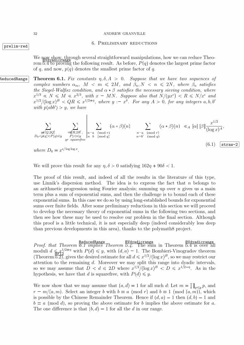
6. Preliminary reductions 32
7. Complete exponential sums 36
8. Incomplete exponential sums 39
9. The Grand Finale 45
10. Weaker hypotheses 52
1991 Mathematics Subject Classification. 11P32.To Yiliang Zhang, for showing that one can, no matter what.
1

2 ANDREW GRANVILLE
1. Introductionsec:intro
1.1. Intriguing questions about primes. Early on in our mathematical educationwe get used to the two basic rules of arithmetic, addition and multiplication. Whenwe define a prime number, simply in terms of the number’s multiplicative properties,we discover a strange and magical sequence of numbers. On the one hand, so easilydefined, on the other, so difficult to get a firm grasp of, since they are defined in termsof what they are not (i.e. that they cannot be factored into two smaller integers)).
When one writes down the sequence of prime numbers:
2, 3, 5, 7, 11, 13, 17, 19, 23, 29, 31, 37, 41, 43, 47, 53, 59, 61, . . .
one sees that they occur frequently, but it took a rather clever construction of theancient Greeks to even establish that there really are infinitely many. Looking furtherat a list of primes, some patterns begin to emerge; for example, one sees that they oftencome in pairs:
3 and 5, 5 and 7, 11 and 13, 17 and 19, 29 and 31, 41 and 43, 59 and 61, . . .
One might guess that there are infinitely many such prime pairs. But this is an open,elusive question, the twin prime conjecture. Until recently there was little theoreticalevidence for it. All that one could say is that there was an enormous amount of com-putational evidence that these pairs never quit; and that this conjecture (and variousmore refined versions) fit into an enormous network of conjecture, which build a beau-tiful elegant structure of all sorts of prime patterns; and if the twin prime conjecturewere to be false then the whole edifice would crumble.
The twin prime conjecture is certainly intriguing to both amateur and professionalmathematicians alike, though one might argue that it is an artificial question, since itasks for a very delicate additive property of a sequence defined by its multiplicativeproperties. Indeed, number theorists had struggled, until very recently, to identify anapproach to this question that seemed likely to make any significant headway. In thisarticle we will discuss these latest shocking developments. In the first few sections wewill take a leisurely stroll through the historical and mathematical background, so asto give the reader a sense of the great theorem that has been recently proved, and alsofrom a perspective that will prepare the reader for the details of the proof.
1.2. Other patterns. Looking at the list of primes above we see other patterns thatbegin to emerge, for example, one can find four primes which have all the same digits,except the last one:
11, 13, 17 and 19, which is repeated with 101, 103, 107 and 109,
and one can find many more such examples – are there infinitely many? More simplyhow about prime pairs with difference 4,
3 and 7, 7 and 11, 13 and 17, 19 and 23, 37 and 41, 43 and 47, 67 and 71, . . . ;
or difference 10,
3 and 13, 7 and 17, 13 and 23, 19 and 29, 31 and 41, 37 and 47, 43 and 53, . . .?

BOUNDED GAPS BETWEEN PRIMES 3
Are there infinitely many such pairs? Such questions were probably asked back toantiquity, but the first clear mention of twin primes in the literature appears in a paperof de Polignac from 1849. In his honour we now call any integer h, for which there areinfinitely many prime pairs p, p h, a de Polignac number.1
Then there are the Sophie Germain pairs, primes p and q : 2p 1, which prove usefulin several simple algebraic constructions:2
2 and 5, 3 and 7, 5 and 11, 11 and 23, 23 and 47, 29 and 59, 41 and 83, . . . ;
Now we have spotted all sorts of patterns, we need to ask ourselves whether there is away of predicting which patterns can occur and which do not. Let’s start by looking atthe possible differences between primes: It is obvious that there are not infinitely manyprime pairs of difference 1, because one of any two consecutive integers must be even,and hence can only be prime if it equals 2. Thus there is just the one pair, 2 and 3, ofprimes with difference 1. One can make a similar argument for prime pairs with odddifference. Hence if h is an integer for which there are infinitely many prime pairs of theform p, q p h then h must be even. We have seen many examples, above, for eachof h 2, h 4 and h 10, and the reader can similarly construct lists of examples forh 6 and for h 8, and indeed for any other even h that takes her or his fancy. Thisleads us to bet on the generalized twin prime conjecture, which states that for any eveninteger 2k there are infinitely many prime pairs p, q p 2k.
What about prime triples? or quadruples? We saw two examples of prime quadruples ofthe form 10n 1, 10n 3, 10n 7, 10n 9, and believe that there are infinitely many.What about other patterns? Evidently any pattern that includes an odd differencecannot succeed. Are there any other obstructions? The simplest pattern that avoids anodd difference is n, n2, n4. One finds the one example 3, 5, 7 of such a prime triple,but no others. Further examination makes it clear why not: One of the three numbersis always divisible by 3. This is very similar to what happened with n, n 1; and onecan verify that, similarly, one of n, n 6, n 12, n 18, n 24 is always divisible by 5.The general obstruction can be described as follows:
For a given set of distinct integers a1 a2 . . . ak we say that prime p is anobstruction if p divides at least one of n a1, . . . , n ak, for every integer n. In otherwords, p divides
Ppnq pn a1qpn a2q . . . pn akqfor every integer n; which can be classified by the condition that the set a1, a2, . . . , akpmod pq includes all of the residue classes mod p. If no prime is an obstruction then wesay that x a1, . . . , x ak is an admissible set of forms.3.
1Pintz makes a slightly definition: That is, that p and p h should be consecutive primes.2These are useful because, in this case, the group of reduced residues mod q is a cyclic group of
order q 1 2p, and therefore isomorphic to C2 Cp if p ¡ 2. Therefore every element in the grouphas order 1 (that is, 1 pmod qq), 2 (that is, 1 pmod qq), p (the squares mod q) or 2p q 1. Henceg pmod qq generates the group of reduced residues if and only if g is not a square mod q and g 1pmod qq.
3Notice that a1, a2, . . . , ak pmod pq can occupy no more than k residue classes mod p and so, if p ¡ kthen p cannot be an obstruction.

4 ANDREW GRANVILLE
Number theorists have long made the optimistic conjecture if there is no such “obvious”obstruction to a set of linear forms being infinitely often prime, then they are infinitelyoften simultaneously prime. That is:
Conjecture: If xa1, . . . , xak is an admissible set of forms then there are infinitelymany integers n such that n a1, . . . , n ak are all prime numbers.
In this case, we call n a1, . . . , n ak a k-tuple of prime numbers.
To date, this has not been proven for any k ¡ 1 though, following Zhang’s work, we arestarting to get close for k 2. Indeed, Zhang proves a weak variant of this conjecture,as we shall see.
The above conjecture can be extended, as is, to all sets of k linear forms with integercoefficients in one variable, so long as we extend the notion of admissibility to alsoexclude the obstruction that two of the linear forms have different signs for all, butfinitely many, n, since a negative integer cannot be prime (for example, n and 2 n);some people call this the “obstruction at the ‘prime’, 1”. We can also extend theconjecture to more than one variable (for example the set of forms m,m n,m 4n):
The prime k-tuplets conjecture: If a set of k linear forms in n variables is admis-sible then there are infinitely many sets of n integers such that when we substitute theseintegers into the forms we get a k-tuple of prime numbers.
There has been substantial recent progress on this conjecture. The famous breakthroughwas Green and Tao’s theorem for the k-tuple of linear forms in the two variables a andd:
a, a d, a 2d, . . . , a pk 1qd.Along with Ziegler, they went on to prove the prime k-tuplets conjecture for any ad-missible set of linear forms, provided no two satisfy a linear equation over the integers.What a remarkable theorem! Unfortunately these exceptions include many of the ques-tions we are most interested in; for example, p, q p 2 satisfy the linear equationq p 2; and p, q 2p 1 satisfy the linear equation q 2p 1).
Finally, we also believe that the conjecture holds if we consider any admissible set ofk irreducible polynomials with integer coefficients, with any number of variables. Forexample we believe that n2 1 is infinitely often prime, and that there are infinitelymany prime triples m, n, m2 2n2.
We will end this section by stating Zhang’s main theorem and a few of the more beguilingconsequences:
Zhang’s main theorem: There exists an integer k such that the following is true: Ifx a1, . . . , x ak is an admissible set of forms then there are infinitely many integersn such that at least two of n a1, . . . , n ak are prime numbers.

BOUNDED GAPS BETWEEN PRIMES 5
Note that the result states that only two of the n ai are prime, not all (as would berequired in the prime k-tuplets conjecture). Zhang proved this result for a fairly largevalue of k, that is k 3500000, which has been reduced to k 632 by the polymath8team. Of course if one could take k 2 then we would have the twin prime conjecture,but the most optimistic plan at the moment, along the lines of Zhang’s proof, wouldyield k 5.
To deduce that there are bounded gaps between primes from Zhang’s Theorem we needonly show the existence of an admissible set with k elements. This is not difficult,simply by letting the ai be the first k primes ¡ k.4 Hence we have proved:
Corollary: [Bounded gaps between primes] There exists a bound B such that there areinfinitely many integers pairs of prime numbers p q pB.
Finding the smallest B for a given k is a challenging question. The prime numbertheorem together with our construction above suggests that B ¤ kplog k Cq for someconstant C, but it is interesting to get better bounds.
Our Corollary further implies
Corollary: There is an integer h, 0 h ¤ B such that there are infinitely many pairsof primes p, p h.
That is, some positive integer ¤ B is a de Polignac number. In fact one can go a littlefurther using Zhang’s main theorem:
Corollary: Let k be as in Zhang’s Theorem, and let A be any admissible set of kintegers. There is an integer h P pA Aq : ta b : a ¡ b P Au such that there areinfinitely many pairs of primes p, p h.
Finally we can deduce from this
Corollary: A positive proportion of integers are de Polignac numbers
Proof. If A t0, . . . , Bu is an admissible set then mA : tma : a P Au is admissiblefor every integer m ¥ 1. Given large x let M rxBs. By Zhang’s Theorem thereexists a pair am bm P A such that mpbm amq is a de Polgnac number. Since thereare at most B2 differences d b a with a b P A there must be some differencewhich is the value of bm am for at least 2MB values of m ¤ M . This gives rise to¥ 2MB ¥ xB2 distinct de Polignac numbers of the form md ¤ x.
Our construction above implies that the proportion is at least 1k2plog k Cq2.
4This is admissible since none of the ai is 0 pmod pq for any p ¤ k, and the p ¡ k were handled inthe previous footnote.

6 ANDREW GRANVILLE
1.3. The simplest analytic approach. There are 14 odd primes up to 50, that is 14out of the 25 odd integers up to 50, so one can deduce that several pairs differ by 2.We might hope to take this kind of density approach more generally: If A is a sequenceof integers of density 12 (in all of the integers) then we can easily deduce that thereare many pairs of elements of A that differ by no more than 2. One might guess thatthere are pairs that differ by exactly 2, but this is by no means guaranteed, as theexample A : tn P Z : n 1 or 2 pmod 4qu shows. Moreover, to use this kind ofreasoning to hunt for twin primes, we presumably need a lower bound on the density ofprimes as one looks at larger and larger primes. This was something that intrigued theyoung Gauss who, by examining Chernik’s table of primes up to one million, surmisedthat “the density of primes at around x is roughly 1 log x” (and this was subsequentlyverified, as a consequence of the prime number theorem). Therefore we are guaranteedthat there are infinitely many pairs of primes p q with q p ¤ log p, which is notquite as small a gap as we are hoping for! Nonetheless this raises the question: Fixc ¡ 0. Can we prove that
There are infinitely many pairs of primes p q with q p c log p ?
This follows for all c ¥ 1 by the prime number theorem, but it is not easy to prove sucha result for any particular value of c 1. The first such results were proved condition-ally assuming the Generalized Riemann Hypothesis. This is, in itself, surprising: TheGeneralized Riemann Hypothesis was formulated to better understand the distributionof primes in arithmetic progressions, so why would it appear in an argument aboutshort gaps between primes? It is far from obvious by the argument used, and yet thisconnection has deepened and broadened as the literature developed. We will discussprimes in arithmetic progressions in detail in the next section.
The first unconditional (though inexplicit) such result, bounding gaps between primes,was proved by Erdos in 1940 using the small sieve (we will obtain any c ¡ eγ 0.5614by such a method in section
MaierTrick3.2 ). In 1966, Bombieri and Davenport
bomdav[2] substituted
the Bombieri-Vinogradov theorem for the Generalized Riemann Hypothesis in earlier,conditional arguments, to prove this unconditionally for any c ¥ 1
2; and in 1988 Maier
maier[25] observed that one can easily modify this to obtain any c ¥ 1
2eγ. The Bombieri-
Vinogradov Theorem is also a result about primes in arithmetic progressions, as we willdiscuss later. Maier further improved this, by combining the approaches of Erdos andof Bombieri and Davenport, to some bound a little smaller than 1
4, with substantial
effort.
The first big breakthrough occurred in 2005 when Goldston, Pintz and Yildirimgpy[15] were
able to show that there are infinitely many pairs of primes p q with q p c log p,for any given c ¡ 0. Indeed they extended their methods to show that, for any ε ¡ 0,there are infinitely many pairs of primes p q for which
q p plog pq12ε.It is their method which forms the basis of the discussion in this paper. Like Bombieriand Davenport, they showed that one can could better understand small gaps betweenprimes, by obtaining strong estimates on primes in arithmetic progressions, as in the

BOUNDED GAPS BETWEEN PRIMES 7
Bombieri-Vinogradov Theorem. Even more, if one assumes a strong, but widely be-lieved, conjecture about the equi-distribution of primes in arithmetic progressions, whichextends the Bombieri-Vinogradov Theorem, then one can show that there are infinitelymany pairs of primes p q which differ by no more than 16 (that is, p q ¤ p 16)!What an extraordinary statement, and one that we will briefly discuss: We know thatif p q ¤ p 16 then q p 2, 4, 6, 8, 10, 12, 14 or 16, and so at least one of thesedifference occurs infinitely often. That is, there exists a positive, even integer 2k ¤ 16such that there are infinitely pairs of primes p, p 2k. Very recently this has beenrefined further by James Maynard, improving the upper bound to 12, by a variant ofthe original argument.
After Goldston, Pintz and Yildirim, most of the experts tried and failed to obtain enoughof an improvement of the Bombieri-Vinogradov Theorem to deduce the existence of somefinite bound B such that there are infinitely many pairs of primes that differ by no morethan B. To improve the Bombieri-Vinogradov Theorem is no mean feat and people havelonged discussed “barriers” to obtaining such improvements. In fact a technique hadbeen developed by Fouvry
fouvry[10], and by Bombieri, Friedlander and Iwaniec
bfi[3], but these
were neither powerful enough nor general enough to work in this circumstance.
Enter Yitang Zhang, an unlikely figure to go so much further than the experts, and tofind exactly the right improvement and refinement of the Bombieri-Vinogradov Theoremto establish the existence of the elusive bound B such that there are infinitely manypairs of primes that differ by no more than B. By all accounts, Zhang was a brilliantstudent in Beijing from 1978 to the mid-80s, finishing with a master’s degree, and thenworking on the Jacobian conjecture for his Ph.D. at Purdue, graduating in 1992. Hedid not proceed to a job in academia, working in odd jobs, such as in a sandwich shop,at a motel and as a delivery worker. Finally in 1999 he got a job at the University ofNew Hampshire as a lecturer, with a high teaching load, working with many of the lessqualified undergraduate students. From time-to-time a lecturer devotes their energy toworking on proving great results, but few have done so with such aplomb as Zhang.Not only did he prove a great result, but he did so by improving technically on theexperts, having important key ideas that they missed and developing a highly ingeniousand elegant construction concerning exponential sums. Then, so as not to be rejectedout of hand, he wrote his difficult paper up in such a clear manner that it could not bedenied. Albert Einstein worked in a patent office, Yitang Zhang in a Subway sandwichshop; both found time, despite the unrelated calls on their time and energy, to thinkthe deepest thoughts in science. Moreover Zhang did so at the relatively advanced ageof 50 (or more). Truly extraordinary.

8 ANDREW GRANVILLE
2. The distribution of primes, divisors and prime k-tuplets
2.1. The prime number theorem. As we mentioned in the previous section, Gaussobserved, at the age of 16, that “the density of primes at around x is roughly 1 log x”,which leads quite naturally to the conjecture that
#tprimes p ¤ xu » x
2
dt
log t x
log xas xÑ 8.
(We use the symbol Apxq Bpxq for two functions A and B of x, to mean thatApxqBpxq Ñ 1 as x Ñ 8.) This was proved in 1896, the prime number theorem,and the integral provides a considerably more precise approximation to the number ofprimes ¤ x, than x log x. However, this integral is rather cumbersome to work with,and so it is natural to instead weight each prime with log p; that is we work with
θpxq :¸
p primep¤x
log p
and the prime number theorem implies5 that
θpxq x as xÑ 8. (2.1) pnt2SieveHeuristic
2.2. A sieving heuristic to guess at the prime number theorem. How manyintegers up to x have no prime factors ¤ y ? If y ¥ ?
x then this counts 1 and all of theprimes between y and x, so an accurate answer would yield the prime number theorem.
The usual heuristic is to start by observing that there are x2 Op1q integers up tox that are not divisible by 2. A proportion 2
3rds of these remaining integers are not
divisible by 3; then a proportion 45ths of the remaining integers are not divisible by 5,
etc. Hence we guess that the number of integers ¤ x which are free of prime factors¤ y, is roughly ¹
p¤y
1 1
p
x.
Evaluating the product here is tricky but was accomplished by Mertens: If y Ñ 8 then¹p¤y
1 1
p
eγ
log y.
Here γ is the Euler-Mascheroni constant, defined as limNÑ8 11 1
2 . . . 1
N logN .
There is no obvious explanation as to why this constant, defined in a very differentcontext, appears here.
If?x y opxq (that is, for any fixed ε ¡ 0 we have y ¤ εx once x is sufficiently
large) then we know from the prime number theorem that there are x log x integersleft unsieved, whereas the prediction from our heuristic varies considerably as y variesin this range. This shows that the heuristic is wrong for large y. Taking y ?
x it
5This is really stating things backwards since, in proving the prime number theorem, it is significantlyeasier to include the log p weight, and then deduce estimates for the number of primes by partialsummation.

BOUNDED GAPS BETWEEN PRIMES 9
predicts too many primes by a factor of 2eγ; taking y x log x it predicts too fewprimes by a factor of eγ. In fact this heuristic gives an accurate estimate providedy xop1q. We will exploit the difference between this heuristic and the correct count,to show that there are smaller than average gaps between primes in section
MaierTrick3.2.
2.3. The prime number theorem for arithmetic progressions, I. Any primedivisor of pa, qq is an obstruction to the primality of values of the polynomial qx a,and these are the only such obstructions. The prime k-tuplets conjecture thereforeimplies that if pa, qq 1 then there are infinitely many primes of the form qn a. Thiswas first proved by Dirichlet in 1837. Once proved one might ask for a more quantitativeresult. If we look at the primes in the arithmetic progressions pmod 10q:
11, 31, 41, 61, 71, 101
3, 13, 23, 43, 53, 73, 83, 103
7, 17, 37, 47, 67, 97, 107
19, 29, 59, 79, 89, 109
then there seem to be roughly equal numbers in each, and this pattern persists as welook further out. Let φpqq denote the number of a pmod qq for which pa, qq 1, and sowe expect that
θpx; q, aq :¸
p primep¤x
pa pmod qq
log p x
φpqq as xÑ 8.
This is the prime number theorem for arithmetic progressions and was first proved bysuitably modifying the proof of the prime number theorem.
The function φpqq was studied by Euler, who showed that it is multiplicative, that is
φpqq ¹peq
φppeq
(where peq means that pe is the highest power of prime p dividing q) and that φppeq pe pe1 for all e ¥ 1.
2.4. Dirichlet’s divisor trick. Another multiplicative function of importance is thedivisor function
τpnq :¸d|n
1
where the sum is over the positive integers d that divide n. It is not difficult to verifythat τppeq e 1.
If n is squarefree and has k prime factors then τpnq 2k, so we see that τpnq variesgreatly depending on the arithmetic structure of n. Nonetheless one might ask for theaverage of τpnq, that is the average number of divisors of a positive integer ¤ x. A first

10 ANDREW GRANVILLE
approach yields that ¸n¤x
τpnq ¸n¤x
¸d|n
1 ¸d|n
¸n¤xd|n
1 ¸d¤x
xd
,
since the positive integers up to x that are divisible by d can be written as dm withm ¤ xd, and so there are rxds such integers, where rts denotes the largest integer ¤ t.It evident that rts tOp1q, where Op1q signifies that there is a correction here of atmost a bounded multiple of 1. If we substitute this approximation in above, we obtain
1
x
¸n¤x
τpnq 1
x
¸d¤x
xdOp1q
¸d¤x
1
dO
1
x
¸d¤x
1
One can approximate°d¤x
1d
by³x1dtt log x. Indeed the difference tends to a limit,
the Euler-Mascheroni constant γ : limNÑ8 11 1
2 . . . 1
N logN . Hence we have
proved that the integers up to x have log x Op1q divisors, on average, which is quiteremarkable for such a wildly fluctuating function.
Dirichlet studied this argument and noticed that when we approximate rxds by xdOp1q for large d, say for those d in px2, xs, then this is not really a very good approxi-mation, and gives a large cumulative error term, Opxq. However we know that rxds 1exactly, for each of these d, and so we can estimate this sum by x2 Op1q, which ismuch more precise. Dirichlet realized that the correct way to formulate this observationis to write n dm, where d and m are integers. When d is small then we should fixd, and count the number of such m, with m ¤ xd (as we did above); but when m issmall, then we should fix m, and count the number of d with d ¤ xm. In this wayour sums are all over long intervals, which allows us to get an accurate approximationof their value. In fact we can exploit the symmetry here to simply “break the sum” atx12. Hence Dirichlet proceeded as follows:¸
n¤xτpnq
¸n¤x
¸dmn
1 ¸d¤?x
¸n¤xd|n
1¸
m ?x
¸n¤xm|n
1¸d¤?x
¸m ?x
1
¸d¤?x
xdOp1q
¸m ?x
xmOp1q
xOp?xq.
One can do even better with these sums than above, showing that°n¤N 1n logN
γ Op1Nq. Hence we can deduce that
1
x
¸n¤x
τpnq log x 2γ 1O
1?x
,
an extraordinary improvement upon the earlier error term.
In the calculations in this article, this same idea is essential. We will take some functions,that are difficult to sum, and rewrite them as a sum of products of other functions, thatare easier to sum, and find a way to sum them over long enough intervals for our methodsto take effect. So we should define the convolution of two functions f and g as f gwhere
pf gqpnq :¸abn
fpaqgpbq,

BOUNDED GAPS BETWEEN PRIMES 11
for every integer n ¥ 1, where the sum is over all pairs of positive integers a, b whoseproduct is n. Hence τ 1 1, where 1 is the function with 1pnq 1 for every n ¥ 1.
Let δ1pnq 1 if n 1, and δ1pnq 0 otherwise. Another important multiplicativefunction is the Mobius function µpnq, since 1 µ δ1. From this one can verify thatµppq 1 and µppeq 0 for all e ¥ 2, for all primes p.
We define Lpnq : log n, and we let Λpnq log p if n is a power of prime p, andΛpnq 0 otherwise. By factoring n, we see that L 1 Λ. We therefore deduce thatΛ pµ 1q Λ µ p1 Λq µ L; that is
Λpnq ¸abn
µpaq log b #
log p if n pm, where p is prime,m ¥ 1;
0 otherwise.. (2.2) VMidentity
We can approach the prime number theorem via this identity by summing over all n ¤ xto get ¸
n¤xΛpnq
¸ab¤x
µpaq log b.
The left-hand side equals θpxq plus a contribution from prime powers pe with e ¥ 2, andit is easily shown that this contribution is small (in fact Op?xq). The right hand sideis the convolution of an awkward function µ and something very smooth and easy tosum, L. Indeed, it is easy to see that
°b¤B log b logB! and we can estimate this very
precisely using Stirling’s formula. One can infer (seeGS[18] for details) that the prime
number theorem is equivalent to proving that
1
x
¸n¤x
µpnq Ñ 0 as xÑ 8.
In our work here we will need a more convoluted identity that (VMidentity2.2) to prove our esti-
mates for primes in arithmetic progressions. There are several possible suitable identi-ties, the simplest of which is due to Vaughan
vaughan[35]:
Vaughan’s identity : Λ¥V µ U L µ U Λ V 1 µ¥U Λ¥V 1 (2.3) Vaughidentity
where g¡W pnq gpnq if n ¡ W and gpnq 0 otherwise; and g g¤W g¡W . To verifythis identity, we manipulate the algebra of convolutions:
Λ¥V Λ Λ V pµ Lq Λ V p1 µq µ U L µ¥U L µ U Λ V 1 µ¥U Λ V 1
µ U L µ U Λ V 1 µ¥U pΛ 1 Λ V 1q,Primektuples
2.5. A quantitative prime k-tuplets conjecture. We are going to develop a heuris-tic to guesstimate the number of pairs of twin primes p, p 2 up to x. We start withGauss’s statement that “the density of primes at around x is roughly 1 log x. Hencethe probability that p is prime is 1 log x, and the probability that p 2 is prime is1 log x so, assuming that these events are independent, the probability that p and p2

12 ANDREW GRANVILLE
are simultaneously prime is
1
log x 1
log x 1
plog xq2 ;
and so we might expect about xplog xq2 pairs of twin primes p, p 2 ¤ x. But thereis a problem with this reasoning, since we are implicitly assuming that the events “pis prime for an arbitrary integer p ¤ x”, and “p 2 is prime for an arbitrary integerp ¤ x”, can be considered to be independent. This is obviously false since, for example,if p is even then p 2 must also be. 6 So, to correct for the non-independence, weconsider the ratio of the probability that both p and p 2 are not divisible by q, to theprobabiliity that p and p1 are not divisible by q, for each small prime q.
Now the probability that q divides an arbitrary integer p is 1q; and hence the probabilitythat p is not divisible by q is 1 1q. Therefore the probability that both of twoindependently chosen integers are not divisible by q, is p1 1qq2.
The probability that q does not divide either p or p 2, equals the probability thatp 0 or 2 pmod qq. If q ¡ 2 then p can be in any one of q 2 residue classes mod q,which occurs, for a randomly chosen p pmod qq, with probability 1 2q. If q 2 thenp can be in any just one residue class mod 2, which occurs with probability 12. Hencethe “correction factor” for divisibility by 2 is
p1 12q
p1 12q2 2,
whereas the “correction factor” for divisibility by any prime q ¡ 2 is
p1 2qq
p1 1qq2 .
Now divisibility by different small primes in independent, as we vary over values of n,by the Chinese Remainder Theorem, and so we might expect to multiply together allof these correction factors, corresponding to each “small” prime q. The question thenbecomes, what does “small” mean? In fact, it doesn’t matter much because the productof the correction factors over larger primes is very close to 1, and hence we can simplyextend the correction to be a product over all primes q. (More precisely, the infiniteproduct over all q, converges.) Hence we define the twin prime constant to be
C : 2¹
q primeq¥3
p1 2qq
p1 1qq2 1.3203236316,
and we conjecture that the number of prime pairs p, p 2 ¤ x is
Cx
plog xq2 .
6Also note that the same reasoning would tell us that there are xplog xq2 prime pairs p, p1 ¤ x.

BOUNDED GAPS BETWEEN PRIMES 13
Computational evidence suggests that this is a pretty good guess. The analogous argu-ment implies the conjecture that the number of prime pairs p, p 2k ¤ x is
C¹p|kp¥3
p 1
p 2
x
plog xq2 .
This argument is easily modified to make an analogous prediction for any k-tuple: Givena1, . . . , ak, let Ωppq be the set of distinct residues given by a1, . . . , ak pmod pq, and thenlet ωppq |Ωppq|. None of the n ai is divisible by p if and only if n is in any one ofp ωppq residue classes mod p, and therefore the correction factor for prime p is
p1 ωppqpq
p1 1pqk .
Hence we predict that the number of prime k-tuplets n a1, . . . , n ak ¤ x is,
Cpaq x
plog xqk where Cpaq :¹p
p1 ωppqpq
p1 1pqk .
An analogous conjecture, via similar reasoning, can be made for the frequency of primek-tuplets of polynomial values in several variables. What is remarkable is that com-putational evidence suggests that these conjectures do approach the truth, though thisrests on a rather shaky theoretical framework. A more convincing theoretical framework(though rather more difficult) was given by Hardy and Littlewood
hardy[19] – see section
HLheuristic3.3.
Recogktuple
2.6. Recognizing prime k-tuples. The identity (VMidentity2.2) allows us to distinguish prime
powers from composite numbers in an arithmetic way. Such identities not only recognizeprimes, but can be used to identify integers with no more than k prime factors. Forexample
Λ2pnq :¸d|nµpdqplog ndq2
$'&'%p2m 1qplog pq2 if n pm;
2 log p log q if n paqb, p q;
0 otherwise.
In general
Λkpnq :¸d|nµpdqplog ndqk
equals 0 if νpnq ¡ k (where νpmq denotes the number of distinct prime factors of m).We will be working with (a variant of) the expression
ΛkpPpnqq.We have seen that if this is non-zero then Ppnq has ¤ k distinct prime factors. We willnext show that if 0 a1 . . . ak and n ¥ a1 . . . ak then Ppnq must have exactly kdistinct prime factors. In that case if the k prime factors of Ppnq are p1, . . . , pk, then
ΛkpPpnqq k!plog p1q . . . plog pkq.

14 ANDREW GRANVILLE
Now, suppose that Ppnq has r ¤ k 1 distinct prime factors, call them p1, . . . , pr. Foreach pi select j jpiq for which the power of pi dividing naj is maximized. Evidentlythere exists some J, 1 ¤ J ¤ k which is not a jpiq. Therefore if peii n aJ then
peii |pn aJq pn ajpiqq paJ ajpiqq, which divides¹
1¤j¤kjJ
paJ ajq.
Hencen aJ lcmi p
eii divides
¹1¤j¤kjJ
paJ ajq,
and so n n aJ ¤±
j aj ¤ n, by hypothesis, which is impossible.
The expression for Λpnq in (VMidentity2.2) can be re-written as
Λpnq ¸d|nµpdq log nd, and even
¸d|nµpdq logRd,
for any R, provided n ¡ 1. Selberg has shown that the truncation¸d|nd¤R
µpdq logRd
is also “sensitive to primes”; and can be considerably easier to work with in variousanalytic arguments. In our case, we will work with the function¸
d|Ppnqd¤R
µpdqplogRdqk,
which is analogously “sensitive” to prime k-tuplets, and easier to work with than thefull sum for ΛkpPpnqq.

BOUNDED GAPS BETWEEN PRIMES 15
3. Uniformity in arithmetic progressions
3.1. When primes are first equi-distributed in arithmetic progressions. Thereis an important further issue when considering primes in arithmetic progressions: Inmany applications it is important to know when we are first guaranteed that the primesare more-or-less equi-distributed amongst the arithmetic progressions a pmod qq withpa, qq 1; that is
θpx; q, aq x
φpqq for all pa, qq 1. (3.1) PNTaps
To be clear, here we want this to hold when x is a function of q, as q Ñ 8.
If one does extensive calculations then one finds that, for any ε ¡ 0, if q is sufficientlylarge and x ¥ q1ε then the primes up to x are equi-distributed amongst the arithmeticprogressions a pmod qq with pa, qq 1, that is (
PNTaps3.1) holds. This is not only unproved
at the moment, also no one really has a plausible plan of how to show such a result.However the slightly weaker statement that (
PNTaps3.1) holds for any x ¥ q2ε, can be shown
to be true, assuming the Generalized Riemann Hypothesis. This gives us a clear planfor proving such a result, but one which has seen little progress in the last century!
The best unconditional results known are much weaker than we have hoped for, equidis-tribution only being proved once x ¥ eq
ε. This is the Siegel-Walfisz Theorem, and it
can be stated in several (equivalent) ways with an error term: For any B ¡ 0 we have
θpx; q, aq x
φpqq O
x
plog xqB
for all pa, qq 1. (3.2) SW1
Or: for any A ¡ 0 there exists B ¡ 0 such that if q plog xqA then
θpx; q, aq x
φpqq"
1O
1
plog xqB*
for all pa, qq 1. (3.3) SW2
That x needs to be so large compared to q limited the number of applications of thisresult.
The great breakthough of the second-half of the twentieth century came in appreciatingthat for many applications, it is not so important that we know that equidistributionholds for every a with pa, qq 1, and every q up to some Q, but rather that this holdsfor most such q (with Q x12ε). It takes some juggling of variables to state theBombieri-Vinogradov Theorem: We are interested, for each modulus q, in the size ofthe largest error term
maxa mod qpa,qq1
θpx; q, aq x
φpqq ,
or even
maxy¤x
maxa mod qpa,qq1
θpy; q, aq y
φpqq .
The bounds 0 ¤ θpx; q, aq ! xq
log x are trivial, the upper bound obtained by bounding
the possible contribution from each term of the arithmetic progression. (Throughoutthe symbol “!”, as in “fpxq ! gpxq” means “there exists a constant c ¡ 0 such that

16 ANDREW GRANVILLE
fpxq ¤ cgpxq.”) We would like to improve on the “trivial” upper bound, perhaps bya power of log x, but we are unable to do so for all q. However, it turns out that wecan prove that if there are exceptional q, then they are few and far between, and theBombieri-Vinogradov Theorem expresses this in a useful form. The first thing we do isadd up the above quantities over all q ¤ Q x. The “trivial” upper bound is then
!¸q¤Q
x
qlog x ! xplog xq2.
The Bombieri-Vinogradov states that we can beat this trivial bound by an arbitrarypower of log x, provided Q is a little smaller than
?x:
The Bombieri-Vinogradov Theorem. For any given A ¡ 0 there exists a constantB BpAq, such that ¸
q¤Qmax
a mod qpa,qq1
θpx; q, aq x
φpqq !A
x
plog xqA
where Q x12plog xqB.
In fact one can take B 2A 5; and one can also replace the summand here by theexpression above with the extra sum over y (though we will not need to do this here).
It is believed that this kind of estimate holds with Q significantly larger than?x; indeed
Elliott and Halberstam conjecturedelliott[8] that one can take Q xc for any constant c 1:
The Elliott-Halberstam conjecture For any given A ¡ 0 and η, 0 η 12, we
have ¸q¤Q
maxa mod qpa,qq1
θpx; q, aq x
φpqq ! x
plog xqA
where Q x12η.
However, it was shown infg-1[13] that one cannot go so far as to take Q xplog xqB.
This conjecture was the starting point for the work of Goldston, Pintz and Yıldırımgpy[15], as well as of Zhang
zhang[38]. This starting point was a beautiful argument from
gpy[15],
that we will spell out in the next section, which yields the following result.
gpy-thm Theorem 3.1 (Goldston-Pintz-Yıldırım).gpy[15] Let k ¥ 2, l ¥ 1 be integers, and 0
η 12, such that
1 2η ¡
1 1
2l 1
1 2l 1
k
. (3.4) thetal
If the Elliott-Halberstam conjecture holds with Q x12η then the following is true: Ifx a1, . . . , x ak is an admissible set of forms then there are infinitely many integersn such that at least two of n a1, . . . , n ak are prime numbers.
The conclusion here is exactly the statement of Zhang’s main theorem.

BOUNDED GAPS BETWEEN PRIMES 17
For now the Elliott-Halberstam conjecture seems too difficult to prove, but progresshas been made when restricting to one particular residue class: Fix integer a 0. Webelieve that for any fixed η, 0 η 1
2, one has¸
q¤Qpq,aq1
θpx; q, aq x
φpqq ! x
plog xqA
where Q x12η. The key to progress has been to notice that if one can“factor” thekey terms here into a sum of convolutions then it is easier to make progress, much as wesaw with Dirichlet and the divisor problem. In this case the key convolution is (
VMidentity2.2) and
Vaughan’s identity (Vaughidentity2.3). A second type of factorization that takes place concerns the
modulus: it is much easier to proceed if we can factor the modulus q as, say dr whered and r are roughly some pre-specified sizes. The simplest class of integers q for whichthis sort of thing is true is the y-smooth integers, those integers whose prime factors areall ¤ y. For example if we are given a y-smooth integer q and we want q dr with dnot much smaller than D, then we select d to be the largest divisor of q that is ¤ D andwe see that Dy d ¤ D. This is precisely the class of moduli that Zhang considered:7
Yitang Zhang’s Theorem There exist constants η, δ ¡ 0 such that for any giveninteger a, we have ¸
q¤Qpq,aq1
q is ysmoothq squarefree
θpx; q, aq x
φpqq !A
x
plog xqA (3.5) EHsmooth
where Q x12η and y xδ.
Zhangzhang[38] proved his Theorem for η2 δ 1
1168, and the argument works provided
414η 172δ 1. We will prove this result, by a somewhat simpler proof, provided162η90δ 1. We expect this estimate holds for every η P r0, 12s and every δ P p0, 1s,but just proving it for any positive pair η, δ ¡ 0 is an extraordinary breakthrough thathas an enormous effect on number theory, since it is such an applicable result (andtechnique). This is the technical result that truly lies at the heart of Zhang’s resultabout bounded gaps between primes, and sketching a proof of this is the focus of thesecond half of this article. starting section
GeneralBV5.
MaierTrick
3.2. A first result on gaps between primes. We will now exploit the differencebetween the heuristic, presented in section
SieveHeuristic2.2, for the prime number theorem, and the
correct count.
Let m ±p¤y p, N m2 and x mN , so that y logm 1
3log x by the prime
number theorem, (pnt22.1). We consider the primes in the short intervals
rmn 1,mn Js for N ¤ n 2N
7We will prove this with ψpx; q, aq :°
n¤x, n¤a pmod qq Λpnq in place of θpx; q, aq. It is not difficult
to show that the difference between the two sums is ! x12op1q.

18 ANDREW GRANVILLE
with J y log y. Note that all of the short intervals are px, 2xs. The total number ofprimes in all of these short intervals is
2N
nN1
πpmn Jq πpmn 1q J
j1
πp2x;m, jq πpx;m, jq ¸
1¤j¤Jpj,mq1
x
φpmq log x
assuming (PNTaps3.1). Hence, since the maximum is always at least the average,
maxnPpN,2Ns
πpmn Jq πpmn 1q ¥ J
log x #t1 ¤ j ¤ J : pj,mq 1u
pφpmqmqJ eγ
J
log x.
using the prime number theorem, and Merten’s Theorem, as in sectionSieveHeuristic2.2. Therefore
we have proved that there is in an interval of length J , between x and 2x, which has atleast J
eγ log xprimes, and so there must be two that differ by À eγ log x.
HLheuristic
3.3. Hardy and Littlewood’s heuristic for the twin prime conjecture. Therather elegant and natural heuristic for the quantitative twin prime conjecture, whichwe described in section
Primektuples2.5, was not the original way in which Hardy and Littlewood
made this extraordinary prediction. The genesis of their technique lies in the circlemethod., that they developed together with Ramanujan. The idea is that one candistinguish the integer 0 from all other integers, since» 1
0
epntqdt #
1 if n 0;
0 otherwise,(3.6) expintegral
where, for any real number t, we write eptq : e2πit. Notice that this is literally anintegral around the unit circle. Therefore to determine whether the two given primes pand q differ by 2, we simply determine» 1
0
eppp q 2qtq dt.
If we sum this up over all p, q ¤ x, we find that the number of twin primes p, p 2 ¤ xequals, exactly,¸
p,q¤xp,q primes
» 1
0
eppp q 2qtq dt » 1
0
|P ptq|2ep2tq dt, where P ptq :¸p¤x
p prime
epptq.
In the circle method one next distinguishes between those parts of the integral whichare large (the major arcs), and those that are small (the minor arcs). Typically themajor arcs are small arcs around those t that are rationals with small denominators.Here the width of the arc is about 1x, and we wish to understand the contribution att am, where pa,mq 1. Note then that
P pamq ¸
b pmod mqpb,mq1
empabqπpx;m, bq.

BOUNDED GAPS BETWEEN PRIMES 19
where empbq ep bmq e2πibm. We note the easily proved identity¸r pmod mq, pr,mq1
emprkq φppk,mqqµpmpm, kqq.
Assuming the prime number theorem for arithmetic progressions with a good error termwe therefore see that
P pamq x
φpmq log x
¸b pmod mqpb,mq1
empabq µpmqφpmq
x
log x.
Hence in total we predict that the number of prime pairs p, p 2 ¤ x is roughly
1
x
¸m¤M
¸a: pa,mq1
emp2aqµpmqφpmq
x
log x
2
x
plog xq2¸m¥1
µpmq2φpmq2 φpp2,mqqµpmp2,mqq
x
plog xq2
1 1
φp2q¹p¡2
1 1
φppq2 C
x
plog xq2 ,
as in sectionquantPrimektuples??. Moreover the analogous argument yields the more general conjecture
for prime pairs p, p h.
Why doesn’t this argument lead to a proof of the twin prime conjecture? For themoment we have little idea how to show that the minor arcs contribute very little.Given that we do not know how to find cancelation amongst the minor arcs, we wouldneed to show that the integrand is typically very small on the minor arcs, meaning thatthere is usually a lot of cancelation in the sums P ptq. For now this is an important openproblem. Nonetheless, it is this kind of argument that has led to Helfgott’s recent proofHH[21] that every odd integer ¥ 3 is the sum of no more than three primes.

20 ANDREW GRANVILLE
4. Goldston-Pintz-Yıldırım’s argumentgpy-sec
We now give a version of the combinatorial argument of Goldston-Pintz-Yıldırımgpy[15],
which was the inspiration for proving that there are bounded gaps between primes:
4.1. The set up. Let H pa1 a2 . . . akq be an admissible k-tuple, and takex ¡ ak. Our goal is to select a function ν for which νpnq ¥ 0 for all n, such that
¸x n¤2x
νpnqpk
i1
θpn aiq log 3xq ¡ 0. (4.1) gpy1
If we can do this then there must exist an integer n such that
νpnqpk
i1
θpn aiq log 3xq ¡ 0.
In that case νpnq 0 so that νpnq ¡ 0, and therefore
k
i1
θpn aiq ¡ log 3x.
However each n ai ¤ 2x ak 2x x and so each θpn aiq log 3x. This impliesthat at least two of the θpn aiq are non-zero, that is, at least two of n a1, . . . , n akare prime.
A simple idea, but the difficulty comes in selecting the function νpnq with these prop-erties for which we can evaluate the sum. In
gpy[15] they had the further idea that they
could select νpnq so that it would be sensitive to when each n ai is prime, or “almostprime”, and so they relied on the type of construction that we discussed in section
Recogktuple2.6.
In order that νpnq ¡ 0 one can simply take it to be a square. Hence we select
νpnq : 1¸d|Ppnq
λpdq
2
where
λpdq : µpdq 1
m!
logRdlogR
mwhen d P D, and λpdq 0 otherwise, for some positive integer m k `, where D is asubset of the squarefree integers in t1, . . . , Ru, and we select R x13. In the argumentof
gpy[15], D includes all of the squarefree integers in t1, . . . , Ru, whereas Zhang uses only
the y-smooth ones. Our formulation works in both cases.
4.2. Evaluating the sums, I. Now, expanding the above sum gives
1
d1,d2D:rd1,d2s
λpd1qλpd2q
k
i1
¸x n¤2xD|Ppnq
θpn aiq log 3x¸
x n¤2xD|Ppnq
1
. (4.2) gpy2

BOUNDED GAPS BETWEEN PRIMES 21
Let ΩpDq be the set of congruence classes m pmod Dq for which D|P pmq; and let ΩipDqbe the set of congruence classes m P ΩpDq with pD,m aiq 1. Hence the parenthesesin the above line equals
k
i1
¸mPΩipDq
¸x n¤2x
nm pmod Dq
θpn aiq log 3x¸
mPΩpDq
¸x n¤2x
nm pmod Dq
1. (4.3) gpy3
The final sum evidently equals xDOp1q; the error term much smaller than the mainterm. We will come back to these error terms a little later. For the first sums we expect(PNTaps3.1) holds, so that each
θp2x;D,m aiq θpx;D,m aiq x
φpDq .
We again neglect, for now, the error terms, and will substitute these two estimates intothe previous line. First though, note that the sets ΩpDq and ΩipDq may be constructedusing the Chinese Remainder Theorem from the sets withD prime. Therefore if ωpDq :|ΩpDq| then ωp.q is a multiplicative function. Moreover each |Ωippq| ωppq 1, whichwe denote by ωppq, and each |ΩipDq| ωpDq, extending ω to be a multiplicativefunction. Putting this altogether we obtain here a main term of
kωpDq x
φpDq plog 3xqωpDq xD x
kωpDqφpDq plog 3xqωpDq
D
.
This is typically negative which is why we cannot simply take our weights to all bepositive. Substituting this in above we obtain, in total, the sums
x
k
1
d1,d2D:rd1,d2s
λpd1qλpd2qωpDqφpDq plog 3xq
1
d1,d2D:rd1,d2s
λpd1qλpd2qωpDqD
. (4.4) gpy4
We shall explain a little later how these were evaluated ingpy[15]. First though let’s return
to the error terms:
4.3. Bounding the error terms. The first one above, from counting integers in anarithmetic progression, yields in total,
!¸
d1,d2¤R|λpd1q||λpd2q| log 3x ¤ R2 log 3x ¤ x23 log 3x,
since each |λpdq| ¤ 1 by definition. For the second one we will need our bound on primesin arithmetic progression: For any integer b we have
1
D¤QpD,bq1
θpX;D, bq X
φpDq !A
X
plogXqA (4.5) PNTassump
where the constant depends only on A. Here Q x12η and the restriction°1 is
vacuous if we assume the Elliott-Halberstam conjecture, and means that D is y-smoothif we are using Zhang’s estimate.

22 ANDREW GRANVILLE
Using the same bounds |λpdq| ¤ 1, we have the upper bound on the second term of
¤1
d1,d2D:rd1,d2s
k
i1
¸mPΩipDq
θp2x;D,m aiq θpx;D,m aiq x
φpDq .
Let OipDq ΩipDq ai (which may also be constructed from the Oippq using theChinese Remainder Theorem). Note that |OipDq| ωipDq ¤ pk 1qωpDq where, here,ωpDq denotes the number of distinct prime factors of D. Each D that appears issquarefree and is ¤ R2, and can occur for at most 3ωpDq pairs d1, d2. Since τpDq 2ωpDq
we deduce that, for A logp3pk 1qq log 2, the above is
¤k
i1
¸Xx or 2x
1
D¤QτpDqA 1
ωipDq¸
bPOipDq
θpX;D, bq X
φpDq (4.6) gpy5
where Q R2.
Now let m be the lcm of the integers D ¤ Q, counted in the sum. Notice that Oipmqreduced mod D, gives ωipmDq copies of OipDq, and hence
1
ωipDq¸
bPOipDq
θpX;D, bq X
φpDq 1
ωipmq¸
bPOipmq
θpX;D, bq X
φpDq ,
so that the quantity in (gpy54.6) equals
k
i1
¸Xx or 2x
1
ωipmq¸
bPOipmq
# 1
D¤QτpDqA
θpX;D, bq X
φpDq+. (4.7) gpy6
Now fix k,X and b. To bound the sum over D we need to remove the τpDqA term,which we do by Cauchying. It will help to notice the trivial bounds 0 ¤ θpX;D, bq !pX logXqD, so that D|θpX;D, bq X
φpDq | ! X logX. Hence 1
D¤QτpDqA
θpX;D, bq X
φpDq2
¤¸D¤Q
τpDq2AD
1
D¤QD
θpX;D, bq X
φpDq2
¤ XplogXqB1
D¤Q
θpX;D, bq X
φpDq
and this is !C X2plogXqC for any C, by (
PNTassump4.5). Hence the quantity in (
gpy54.6) is
!A kX
plogXqA ,
for any A ¡ 0, which is acceptable.
4.4. Perron’s formula. There are two methods to calculate the main terms, one moreanalytic (
gpy[15]), the other, (
sound[34],
ggpy[16]), more combinatorial. We shall outline both.
It is possible to obtain an asymptotic estimate for the mean value of multiplicativefunctions g for which gppq is “close” to some given integer k, for all sufficiently large p.

BOUNDED GAPS BETWEEN PRIMES 23
The Selberg-Delange theorem tells us that¸n¤x
gpnqn
¹p¤x
1 gppq
p gpp2q
p2 . . .
1 1
p
k plog xqk
k!.
When gppq is sufficiently close to some k that the Euler product converges, we canreplace the product up to x, by the product over all primes p in the line above. Thismakes this formula easy to manipulate; in particular, by partial summation, we obtain¸
n¤x
gpnqn
plogpxnqq``!
Cpgq plog xqk`pk `q! (4.8) SD+
for k ¥ 1, ` ¥ 0 using the beta integral³10p1 vq`vk1dv pk 1q!`!pk `q!, where
Cpgq :¹
p prime
1 gppq
p gpp2q
p2 . . .
1 1
p
k.
4.5. The combinatorial approach. We will suppose for now that the Λpdq remainunchosen. We need to evaluate the sums
1
d1,d2D:rd1,d2s
λpd1qλpd2qωpDqφpDq and
1
d1,d2D:rd1,d2s
λpd1qλpd2qωpDqD
.
As shown by Soundararajansound[34], we may evaluate these much like Selberg does in his
upper bound sieve. The main idea is a change of variable: Let φω be the multiplicativefunction (defined here, only on squarefree integers) for which φωppq p ωppq, andthen
yprq : µprqφωprqωprq
1
n: r|n
λpnqωpnqn
;
and one can verify this is invertible with
λpdq µpdq d
ωpdq1
n: d|n
ypnqωpnqφωpnq
Now1
d1,d2D:rd1,d2s
λpd1qλpd2qωpDqD
1
d1,d2D:rd1,d2s
ωpDqD
µpd1q d1
ωpd1q1
r: d1|r
yprqωprqφωprq µpd2q d2
ωpd2q1
s: d2|s
ypsqωpsqφωpsq
¸r,s
yprqωprqφωprq
ypsqωpsqφωpsq
1
d1,d2d1|r, d2|s
µpd1qµpd2q pd1, d2qωppd1, d2qq
By writing dj ejfj where ej|pr, sq and f1|rpr, sq, f2|spr, sq, we see that the sum overfj equals 0 unless rpr, sq spr, sq 1; that is r s. Hence the above is
¸r,
yprq2ωprq2φωprq2
1
d1,d2|rµpd1qµpd2q pd1, d2q
ωppd1, d2qq

24 ANDREW GRANVILLE
Letting g pd1, d2q and writing d1 ge1, d2 ge2, so ge1e2|r, we see that the sumover e2 is 0 unless r ge1. The above becomes
1
d1,d2D:rd1,d2s
λpd1qλpd2qωpDqD
¸r
yprq2ωprq2φωprq2
¸g|r
g
ωpgqµprgq ¸r
yprq2ωprqφωprq . (4.9) solve1
One can similarly show that
1
d1,d2D:rd1,d2s
λpd1qλpd2qωpDqφpDq
¸r
yprq2ωprqφωprq (4.10) solve2
where
yprq r1
n: r|n
ypnqφpnq .
We select
yprq y`prq :#Cpaq plogpRrqq`
`!if r is squarefree, and r ¤ R;
0 otherwise,
in the notation of sectionPrimektuples2.5. By (
SD+4.8) this implies that
yprq y`1prq;
λpdq #t1 op1quµpdq plogpRdqqk`
pk`q! if d is squarefree, and d ¤ R;
0 otherwise.
Moreover (SD+4.8) also implies that
(solve14.9) Cpaq
2`
`
plogRqk2`
pk 2`q!and
(solve24.10) Cpaq
2` 2
` 1
plogRqk2`1
pk 2` 1q!
4.6. Finding a positive difference; the proof of Theoremgpy-thm3.1. Now inserting
these last two estimates into (gpy44.4) we obtain
x
t1 op1qu k
pk 2` 1q!
2` 2
` 1
CpaqplogRqk2`1
t1 op1quplog 3xq 1
pk 2`q!
2`
`
CpaqplogRqk2`
¥ Cpaqx log 3x
4plogRqk2`
k
pk 2` 1q!
2` 2
` 1
2 logQ
log 3x
1 1
2` 1
1 2` 1
k
op1q
as Q R2. This is ¡ 0 if (
thetal3.4) holds, and so we deduce Theorem
gpy-thm3.1.

BOUNDED GAPS BETWEEN PRIMES 25
4.7. The challenge in completing the proof of Zhang’s Theorem. We modifythe proof in the last section suitably. In the arguments above we replace y and y, byz and z, where we select
zprq z`prq :#Cpaq plogpRrqq`
`!if r is squarefree, y-smooth and r ¤ R;
0 otherwise,
We bound (solve14.9)(with z in place of y) from above, trivially, as follows:
¸r
zprq2ωprqφωprq ¤
¸r
yprq2ωprqφωprq Cpaq
2`
`
plogRqk2`
pk 2`q! ,
from the calculation in the previous section.
To bound (solve24.10)(with z in place of y) from below, is more subtle. Notice that each term
is ¥ 0, so we have a lower bound by restricting attention to only those r P rRy,Rswhich are y-smooth. Now if ypnq 0 and r|n then nr ¤ Rr ¤ y, and so n is y-smooth;hence
zprq r¸n: r|n
n is y-smooth
zpnqφpnq r
¸n: r|n
n is y-smooth
ypnqφpnq r
1
n: r|n
ypnqφpnq yprq.
Therefore
¸r
zprq2ωprqφωprq ¥
¸Ry¤r¤R
zprq2ωprqφωprq
¸Ry¤r¤R
r is y-smooth
yprq2ωprqφωprq
¥¸
Ry¤r¤R
yprq2ωprqφωprq
1
¸p|rp¡y
1
¥¸r¤R
yprq2ωprqφωprq
¸r¤Ry
yprq2ωprqφωprq
¸p¡y
¸r¤Rp|r
yprq2ωprqφωprq
Now, by (SD+4.8), we have
¸r¤Rp|r
yprq2ωprqφωprq ωppq 1
p 1 Cpaq
2` 2
` 1
plogRpqk2`1
pk 2` 1q!
Summing this over y p ¤ R, and as ωppq ¤ k and Rp ¤ Ry we deduce that
¸p¡y
¸r¤Rp|r
yprq2ωprqφωprq À pk 1q logp1δqp1 δqk2`1 Cpaq
2` 2
` 1
plogRqk2`1
pk 2` 1q!

26 ANDREW GRANVILLE
If one proceeds as in the proof of (SD+4.8) (i.e. by partial summation) one obtains
¸r¤Ry
yprq2ωprqφωprq
³1δ0
p1 vq2`vk1dv³10p1 vq2`vk1dv
¸r¤R
yprq2ωprqφωprq
À pk 2`q!pk 1q!p2`q!p1 δqk1 Cpaq
2` 2
` 1
plogRqk2`1
pk 2` 1q!Assuming that ` ?
k, we deduce that¸r
zprq2ωprqφωprq Á t1Opk2`1p1 δqkquCpaq
2` 2
` 1
plogRqk2`1
pk 2` 1q!
Proceeding as in the previous section (with z in place of y) and taking Q x12η with
L 2` 1 ?k, we are successful provided
1 2η ¡ 1 2
LOp1k kLp1 δqkq op1q,
which works for δ p2L log kqk and η 2L.
4.8. Numerics. Later we will show that we may work here under the assumption that162η 90δ 1. The above inequalities hold (more-or-less) with L 863, k L2 andη 1pL 1q. Hence we should be able to take k ¤ 750, 000 and B 107.
Remark 4.1. These arguments actually give quantitative information: One can deduce(pintz-polignac[29],
maynard[26]) that if H is an admissible k-tuple and x is sufficiently large, then there are
" x logk x values of n P rx, 2xs such that nH contains two primes. In justifying ourweights we claimed that they are “sensitive” to all of the elements of nH being prime:To be more explicit, one can further prove that all of the elements of n H have noprime factors less than xc (for some fixed c ¡ 0), as well as two of them being prime.

BOUNDED GAPS BETWEEN PRIMES 27
5. Distribution in arithmetic progressionsGeneralBV
Our goal, in the rest of the article, is to prove (PNTassump4.5). In this section we will see how
this question fits into a more general framework, as developed by Bombieri, Friedlanderand Iwaniec
bfi[3], so that the results here should allow us to deduce analogous results for
interesting arithmetic sequences other than the primes.
5.1. General sequence in arithmetic progressions with large common differ-ences. One can ask whether any given sequence pβnqn¥1 P C is well-distributed inarithmetic progressions. To this end we might ask that it is well-distributed in a rangeanalogous to (
SW13.2). Therefore we say that β satisfies a Siegel-Walfisz condition if, for
any fixed A ¡ 0, and whenever pa, qq 1, we have¸n¤x
na pmod qq
βn 1
φpqq¸n¤x
pn,qq1
βn
!Aβx 1
2
plog xqA ,
with β β2 where, as usual,
βp :¸n¤x
|βn|p 1
p
.
It is necessary to have a term like β on the right-hand side to account for the size ofthe terms of the sequence β. 8 Note that this estimate is trivial if q ¥ plog xq2A (afterCauchying), so is only of interest for x very large compared to q.
Using the large sieve, Bombieri, Friedlander and Iwaniecbfi[3] were able to prove two
extraordinary results. In the first they showed that if β satisfies a Siegel-Walfisz con-dition,9 then it is well-distributed for almost all arithmetic progressions a pmod qq, foralmost all q ¤ xplog xqB:
Theorem 5.1. Suppose that the sequence of complex numbers βn, n ¤ x satisfies aSiegel-Walfisz condition. For any A ¡ 0 there exists B BpAq ¡ 0 such that
¸q¤Q
¸a: pa,qq1
¸
na pmod qqβn 1
φpqq¸
pn,qq1
βn
2
! β2 x
plog xqA
where Q xplog xqB.
The analogous result for Λpnq is known as the Barban-Davenport-Halberstam theoremand in this case one can even obtain an asymptotic.
8Analogously, we might have used βrx1 1
r for any r ¡ 1 in place of βx12 . This bound is trivial
for q ¥ plog xqArpr1q by Holdering (instead of Cauchying).9Their condition appears to be weaker than that assumed here, but is actually equivalent by LemmaSWcoprime
6.2.

28 ANDREW GRANVILLE
In the second result they show that rather general convolutions are well-distributed forall arithmetic progressions a pmod qq, for almost all q ¤ x12plog xqB:
BFI2 Theorem 5.2. Suppose that we have two sequences of complex numbers αm, M m ¤ 2M , and βn, N n ¤ 2N , where βn satisfies the Siegel-Walfisz condition. For anyA ¡ 0 there exists B BpAq ¡ 0 such that
¸q¤Q
maxa: pa,qq1
¸
na pmod qqpα βqpnq 1
φpqq¸
pn,qq1
pα βqpnq ! αβ x12
plog xqA
where Q x12plog xqB, provided x MN with xε !M,N ! x1ε.
In fact their proof works provided N ¥ exppplog xqεq and M ¥ plog xq2B4.
This allowed them to give a proof of the Bombieri-Vinogradov theorem for primes thatseems to be less dependent on very specific properties of the primes (as we will see inthe next subsection). The subject, though, had long been stuck with the bound x12 onthe moduli.10
Bombieri, Friedlander and Iwaniecbfi[3] made the following conjecture.11 They noted that
in many applications, it suffices to work with a fixed (as is true in the application here).
Conjecture 5.3. Suppose that we have two sequences of complex numbers αm, M m ¤ 2M , and βn, N n ¤ 2N , where βn satisfies the Siegel-Walfisz condition. For anyA, ε ¡ 0, and every integer a, we have
¸q¤Q
pq,aq1
¸
na pmod qqpα βqpnq 1
φpqq¸
pn,qq1
pα βqpnq ! αβ x12
plog xqA
where Q x1ε, provided x MN with xε !M,N ! x1ε.
The extraordinary work of Zhang breaks through the?x barrier in some generality,
working with moduli slightly larger than x12. In this case the moduli are y-smooth,with y xδ; here we say that q is y-smooth if all of its prime factors are ¤ y, that isP pqq ¤ y, where we write P pqq for q’s largest prime factor.
We say that α β satisfies the average sieving condition if for each fixed A ¡ 0, we have¸q Q
¸x mn¤xxplog xqAmna pmod qq
|αm||βn| !A αβ x12
plog xqA plog xqOp1q.
10There had been some partial progress with moduli ¡ x12, as inbfi-2[4], but no upper bounds which
“win” by an arbitrary power of log x (which is what is essential to applications).11They actually conjectured that one can take Q xplog xqB . They also conjectured that if one
assumes the Siegel-Walfisz condition with βsN1 1
s in place of βN12 then we may replace αβx12
in the upper bound here by αM1 1r βN1 1
s .

BOUNDED GAPS BETWEEN PRIMES 29
for any Q x23. We say that α β satisfies the necessary sieving condition if bothα β and α4 β4 satisfy the average sieving condition. It is not difficult to show thatthese conditions hold if, for instance, |αpnq|, |βpnq| ! pτpnq log xqOp1q for all n.
The key result is as follows:
BVdyadicrange Theorem 5.4. There exist constants η, δ ¡ 0 with the following property. Suppose thatwe have two sequences of complex numbers αm, M m ¤ 2M , and βn, N n ¤ 2N ,where β satisfies the Siegel-Walfisz condition, and that α β satisfies the necessarysieving condition. For any A ¡ 0, for any integer a,
¸q¤Q
P pqq¤xδpq,aq1
q squarefree
¸
na pmod qqpα βqpnq 1
φpqq¸
pn,qq1
pα βqpnq !A αβ x12
plog xqA
where Q x12η, provided x13 ! N ¤M ! x23.
BVwiderange Corollary 5.5. There exist constants η, δ ¡ 0 with the following property. Supposethat we have two sequences of complex numbers αm, βn x13 m,n ¤ x23, whichboth uniformly satisfy the Siegel-Walfisz condition, and that α β satisfies the necessarysieving condition. For any A ¡ 0, for any integer a,
¸q¤Q
P pqq¤xδpq,aq1
q squarefree
¸n¤x
na pmod qq
pα βqpnq 1
φpqq¸n¤x
pn,qq1
pα βqpnq
!A αβ x12
plog xqA
where Q x12η.
Proof. of CorollaryBVwiderange5.5 Theorem
BVdyadicrange5.4 gives the result when the support for both α and
β are within dyadic intervals. Here we deduce the result over wider ranges of m and nwith mn ¤ x for some given x.
Let T plog xqA, and R be the smallest integer with p11T qR ¡ x. Let Si,j be the setof pairs pm,nq with p11T qi ¤ m p11T qi1, p11T qj ¤ n p11T qj1. Noticethat if i j ¤ R 3 and pm,nq P Si,j then mn ¤ p1 1T qij2 ¤ p1 1T qR1 ¤ x.Finally let S0 be the set of pairs pm,nq with mn ¤ x, that are not included in any of theSi,j with ij ¤ R3. If pm,nq P S0 thenmn ¥ p11T qij ¥ p11T qR2 ¥ xp13T q.
Now, by the triangle inequality, the sum over all pairs m,n is bounded by the sum, foreach such set S, over the sums for pm,nq P S. For any S of the form Si,j we use TheoremBVdyadicrange5.4 with A replaced by 3A 2. For S S0 we get the bound from the hypothesis thatα β satisfies the average sieving condition. The result follows from summing thesebounds.

30 ANDREW GRANVILLE
5.2. Vaughan’s identity, and the deduction of the main theorems for primes.We will bound each term that arises from Vaughan’s identity, (
Vaughidentity2.3), rewritten as,
Λ Λ V µ U L µ U Λ V 1 µ¥U Λ¥V 1.
To start with, note that¸q Q
¸naq pmod qq
Λ V pnq ¤¸q Q
V
q 1
log V ! V log2 xQ log x
which is an acceptable error term when we let U V x13, with Q x23op1q.
Next we estimate the second term in Vaughan’s identity:¸x n¤2x
na pmod qq
pµ U Lqpnq ¸u U
pu,qq1
µpuq¸
xu m¤2xumau pmod qq
Lpmq
¸u U
pu,qq1
µpuqx
uqplog
4x
u 1q Oplog xq
.
By averaging over all arithmetic progressions a mod q with pa, qq 1, we obtain thesame estimate for 1φpqq times the same sum over n with pn, qq 1. Therefore thedifference is¸
x n¤2xna pmod qq
pµ U Lqpnq 1
φpqq¸
x n¤2xpn,qq1
pµ U Lqpnq !¸u U
pu,qq1
log x ! U log x.
Now summing over all q ¤ Q, yields a contribution of ! UQ log x ! xplog xqA for anyA.
We will further write
µ U Λ V 1 µ U Λ V 1 UV pµ Λq U 1¥UV ,
and we now deal with the second part, much as the above, noting that |pµ Λq Upuq| ¤|p1 Λq Upuq| ¤ log u ¤ log x:¸
x n¤2xna pmod qq
ppµ Λq U 1¥UV qpnq ¸u U
pu,qq1
pµ Λq Upuq¸
maxtxu,UV u m¤2xumau pmod qq
1
¸u U
pu,qq1
pµ Λq Upuq
1
qp2xumaxtxu, UV uq Oplog xq
,
from which we deduce, by averaging over all arithmetic progressions a mod q withpa, qq 1,¸
x n¤2xna pmod qq
ppµΛq U1¥UV qpnq 1
φpqq¸
x n¤2xpn,qq1
ppµΛq U1¥UV qpnq !¸u U
pu,qq1
log x ! U log x.
Now summing over all q ¤ Q, yields a contribution of ! UQ log x ! xplog xqA for anyA.

BOUNDED GAPS BETWEEN PRIMES 31
We are now left to work with two sums of convolutions:¸mnx
mna pmod qq
pµ U Λ V qpmq1 UV pnq and¸mnx
mna pmod qq
pΛ¥V 1qpmqµ¥Upnq,
where x13 ! m,n ! x23, and each convolution takes the form αpmqβpnq where |αpmq| ¤logm, |βpnq| ¤ 1, α and β satisfy the Siegel-Walfisz criterion,12 and α β satisfies thenecessary sieving condition (since . We can therefore apply Corollary
BVwiderange5.5 to each such
sum, and the result follows.
12We need to change things a bit since SW is not known for the convolution. Some version can bededuced though with upper bound in terms of the 2-norms of the two original sequences, rather thanthe 2-norm of the convolution.
32 ANDREW GRANVILLE
6. Preliminary reductionsprelim-red
We now show, through several straightforward manipulations, how we can reduce Theo-rem
BVdyadicrange5.4 to proving the following result. As before, P pqq denotes the largest prime factor
of q, and now, ppqq denotes the smallest prime factor of q.
ReducedRange Theorem 6.1. Fix constants η, δ, A ¡ 0. Suppose that we have two sequences ofcomplex numbers αm, M m ¤ 2M , and βn, N n ¤ 2N , where βn satisfiesthe Siegel-Walfisz condition, and α β satisfies the necessary sieving condition, wherex13 ! N ¤ M ! x23, with x MN . Suppose also that Npyxεq R ¤ Nxε andx12plog xqB QR ¤ x12η, where y : xδ. For any A ¡ 0, for any integers a, b, b1
with ppabb1q ¡ y, we have
¸qPrQ,2Qs
D0 ppqq¤P pqq¤y
¸rPrR,2Rs,P prq¤y
qr squarefree
¸
na pmod rqnb pmod qq
pα βqpnq ¸
na pmod rqnb1 pmod qq
pα βqpnq
!A αβ x12
plog xqA ,
(6.1) straw-2
where D0 xε log log x.
We will prove this result for any η, δ ¡ 0 satisfying 162η 90δ 1.
The proof of this result, and indeed of all the results in the literature of this type,use Linnik’s dispersion method. The idea is to express the fact that n belongs toan arithmetic progression using Fourier analysis; summing up over n gives us a mainterm plus a sum of exponential sums, and then the challenge is to bound each of theseexponential sums. In this case we do so by using long-established bounds for exponentialsums over finite fields. After some preliminary reductions in this section we will proceedto develop the necessary theory of exponential sums in the following two sections, andthen see how these may be used to resolve our problem in the final section. Althoughthis proof is a little technical, it is not especially deep (indeed considerably less deepthan previous developments in this area), thanks to the polymath8 project.
Proof. that TheoremReducedRange6.1 implies Theorem
BVdyadicrange5.4. The sum in Theorem
BVdyadicrange5.4 is over all
moduli d ¤ x12η with P pdq ¤ y, with pd, aq 1. The Bombieri-Vinogradov theorem(Theorem
BFI25.2), gives the desired estimate for all d ¤ x12plog xqB, so we may restrict our
attention to the remaining d. Moreover we may split this range into dyadic intervals,so we may assume that D d ¤ 2D where x12plog xqB D ¤ x12η. As in thehypothesis, we have that d is squarefree, with P pdq ¤ y.
We now show that we may assume that pa, dq 1 for all such d: Let m ±p¤y p, and
r mpa,mq. Select an integer b with b a pmod rq and b 1 pmod pa,mqq, whichis possible by the Chinese Remainder Theorem. Hence if pd, aq 1 then pd, bq 1 andb a pmod dq, so proving the above estimate for b implies the above estimate for a.The one difference is that pb, dq 1 for all the d in our range.

BOUNDED GAPS BETWEEN PRIMES 33
Next we show that we may restrict our attention to those d with νpdq ¤ C log log x,that is that have ¤ C log log x prime factors. By Cauchying twice, the square of¸
D d¤2DP pdq¤xδ
νpdq¡C log log xd squarefree
¸na pmod dq
|pα βqpnq|, (6.2) Cautwice
is
¤¸
D d¤2Dνpdq¡C log log x
1 ¸
D d¤2DP pdq¤xδ
x
D
¸na pmod dq
|pα βqpnq|2.
To bound the first term here we use the Hardy-Ramanujan result that¸n¤x
νpnqk
1 ! x
log x
plog log xOp1qqk1
pk 1q! .
To bound the second term we note that |pαβqpnq|2 ¤ τpnqp|α|2 |β|2qpnq by Cauchying,so that ¸D d¤2D
¸na pmod dq
|pα βqpnq|2
2
¤¸
D d¤2D
¸na pmod dq
τpnq3¸
D d¤2D
¸na pmod dq
p|α|4|β|4qpnq;
which implies that¸D d¤2D
¸na pmod dq
|pα βqpnq|2 ! α28β2
8 x34plog xqOp1q.
by using the average sieving condition for α4 β4 with A 0. hence the quantity in(Cautwice6.2) is
!
D
plog xqCplogC1q1 xD α2
8β28 x
34plog xqOp1q12
! α8β8 x78
plog xqA ,
by taking C sufficiently large. Now αβ x12 ¤ α8β8 x78 by Holder’s inequality,
and we should really state our result in terms of these 8-norms. But for now we willassume that α8β8 x
78 ! αβ x12plog xqOp1q so we can express our result in termsof 2-norms.13
The reason for restricting the values of d as in the last paragraph is that it allows us tofactor d in a convenient way. If d p1p2 . . . pm with p1 p2 . . . pm then select r ofthe form p1p2 . . . p` as large as possible with r ¤ Nxε. Evidently r ¡ Npyxεq ¡ x14.
Note also that p` ¡ D0, else r ¤ D`0 ¤ D
νpdq0 ¤ DC log log x
0 xCε x14 if ε were chosen
13If we Cauchy instead by taking |pα βqpnq|2 ¤ p1 |α|2qpnqp1 |β|2qpnq then
α β4 ¤
¸n
p1 |α|2qpnqp1 |β|2qpnq
2
¤¸n
τpnqp1 |α|4qpnq ¸n
τpnqp1 |β|4qpnq.
The first term in this product is°
a |αpaq|4°
n: a|n τpnq !°
a |αpaq|4τpaq N logN. We eventually show
that α β ¤ α8β8 x38plog xq54.

34 ANDREW GRANVILLE
sufficiently small. Writing d qr we see that ppqq ¡ p` ¡ D0. Hence there exists R andQ as in the hypothesis of Theorem
ReducedRange6.1 with
q P rQ, 2Qs, D0 ppqq ¤ P pqq ¤ y and r P rR, 2Rs, P prq ¤ y.
We will apply the factorization, with γ α β¸na pmod qrq
γpnq 1
φpqrq¸
pn,qrq1
γpnq
¸na pmod qqna pmod rq
γpnq 1
φpqq¸
pn,qq1na pmod rq
γpnq 1
φpqq
¸
pn,qq1na pmod rq
γpnq 1
φprq¸
pn,qq1pn,rq1
γpnq
For the first terms we apply TheoremReducedRange6.1 with b a, for each b1 pmod qq with pb1, qq 1,
and average, to obtain by the triangle inequality
¸qPrQ,2Qs
D0 ppqq¤P pqq¤y
¸rPrR,2Rs,P prq¤y
¸
na pmod qqna pmod rq
γpnq 1
φpqq¸
pn,qq1na pmod rq
γpnq
!A αβ x12
plog xqA ,
(6.3) straw-3
For the second terms we take absolute values and sum over q and r separately to obtainthe upper bound
¤¸
q¤x12
1
φpqq¸
r¤x12ε
¸
pn,qq1na pmod rq
γpnq 1
φprq¸
pn,qq1pn,rq1
γpnq
.
Now in LemmaSWcoprime6.2 below, we show that βn1pn,qq1 satisfies a Siegel-Walfisz condition,
since βn does. By TheoremBFI25.2 (with α and β replaced by αn1pn,qq1 and βn1pn,qq1,
respectively), we deduce that γn1pn,qq1 satisfies a Bombieri-Vinogradov Theorem. Sub-stituting this into the last equation gives
!A
¸q¤x12
1
φpqqαβx12
plog xqA1
and the result follows.
SWcoprime Lemma 6.2. If βn satisfies a Siegel-Walfisz condition then for any m ¥ 1 we have¸
na pmod qqpn,mq1
βn 1
φpqq¸
n: pn,mqq1
βn
! τpmqβ N
12
plogNqC .
Proof. of LemmaSWcoprime6.2 We may assume that q ¤ plogNq2C else, by Cauchying,
¸na pmod qq
pn,mq1
βn
2
¤¸
na pmod qq1 ¸n
|βn|2 ¤ N
qβ2;

BOUNDED GAPS BETWEEN PRIMES 35
And then, by averaging this over all a with pa, qq 1, one deduces the result providedq ¡ plogNq2C .
Now for an arbitrary m we decompose the sum as¸na pmod qq
pn,mq1
βn ¸d|m
µpdq¸
na pmod qqd|n
βn
and, Cauchying, the square of the sum here, over d ¥ plogNq2C , is
¤ τpmq¸d|m
d¥plogNq2C
β2N
dq¤ τpmq2β2 N
plogNq2C .
For the smaller d we use the identity¸na pmod qqn0 pmod dq
βn ¸r|dµprq
¸b: pb,rq1
¸na pmod qqnb pmod rq
βn.
Applying the Siegel-Walfisz condition for each such modulus qr (with C replaced by6C) we obtain an upper bound¸
d plogNq2C
¸r|dφprqβ N
12
plogNq6C ! β N12
plogNqC .

36 ANDREW GRANVILLE
7. Complete exponential sumsexp-sec
In sectionHLheuristic3.3 we developed some notation for exponentials, for example eqpaq epa
qq.
For a rational number ab we have to be a little more careful in defining eqpabq: If bhas a factor in common with q then define eqpabq 0. If pb, qq 1, select c pmod qq sothat bc a pmod qq and then define eqpabq eqpcq, and note that this is well-defined.
In this section we will obtain upper bounds for°n eqpfpnqq where fpxq is a rational
function, and the sum is over all n P pZqZq for which the denominator of fpnq iscoprime to q. By a rational function we mean that fpxq P pxqQpxq for some P,Q PZrxs and we define deg f maxpdegP, degQq. We will then derive such bounds, forsquarefree q, from bounds for primes p, using the following consequence of the Chineseremainder theorem yields: If q1, . . . , qk are pairwise coprime natural numbers, then forany integer a and q : q1 . . . qk we have
eqpaq k¹j1
eqj
a
pqqjq. (7.1) CRTgeneral
In particular this implies that¸nPZqZ
eqpfpnqq ¹p|q
¸nPZpZ
ep
fpnqpqpq
. (7.2) CRTexpsum
7.1. Two special cases. If fpxq ax b then
¸x
eqpax bq eqpbqq1
j0
e
aj
q
#q eqpbq if q divides a;
0 otherwise ,
the discrete analogue of (expintegral3.6). If fpxq cpx dq with c 0 pmod pq, then we make
the change of variable x cy d, which is a bijection from x P Fpztdu Ñ y P Fpzt0u,so that ¸
xPZpZep
c
x d
¸y0
eppyq 1. (7.3) inversesum
This can be combined with (CRTexpsum7.2) to deduce the following (see
zhang[38, Proposition 11]):
dork Lemma 7.1. Let d1, d2 be natural numbers with rd1, d2s square-free, and let c1, c2, l1, l2be integers. Then
¸nPZrd1,d2sZ
ed1
c1
n l1
ed2
c2
n l2
¤ pc1, d11qpc2, d
12qpd1, d2q
where d1i : dipd1, d2q for i 1, 2.
Proof. We will prove the p-component of this bound for each prime divisor p of rd1, d2s,and then deduce the full result using the Chinese Remainder Theorem, as in (
CRTexpsum7.2), as
the right-hand side of our bound is a multiplicative function.

BOUNDED GAPS BETWEEN PRIMES 37
The bound is trivial if pc1, d11q, pc2, d
12q, or pd1, d2q is equal to p, since there are no more
than p terms in the sum, so we may assume without loss of generality that d1 p,d2 1, and c1 is coprime to p. The result then follows immediately from (
inversesum7.3).
Notice that this bound is probably improvable, since we have not exploited any possiblecancelation in the sums for the primes that divide pd1, d2q.
7.2. The deeper theory of exponential sums. In general there is some significantcancelation in exponential sums, and we now discuss those deeper results (due primarilyto Weil) that we need. In fact one can as easily state rather general results, but we willonly use those results when f takes the form
a
x cx, or
a
x b
x ` cx, or
a
xpx kq b
px `qpx ` kq cx (7.4) needExpSums
for any given integers a, b, c, k, `, with k, ` 0 pmod pq.
The Weil conjectures for curvesweil[37] (proven for arbitrary varities by Deligne in
WeilII[7]),
imply “square root cancellation” for various natural exponential sums over finite fields(note that ZpZ is isomorphic to the finite field Fp).
prime-exp Lemma 7.2. If p is prime p and fpxq is a rational function in FprXs of degree d, with1 ¤ d p, then
¸xPFp
ep pfpxqq ! d
?p. (7.5) pqp
This bound follows from the Weil conjectures applied to yp y P pxqQpxq in Fp. Anelementary proof based on Stepanov’s method may also be found in
cochrane[6].
Setting d p is natural, in that, for examples like fpxq gpxqp gpxq c, we see thatfpnq pmod pq is constant by Fermat’s little theorem, so there would be no cancelationin the exponential sum.
We do not need to obtain the full square root cancellation in (pqp7.5) in our work here:
Any bound of the form pc for some fixed c 23
would suffice in our argument. Thisgives hope that there may be a more elementary argument.
We next extend Lemmaprime-exp7.2 to square-free moduli:
For q an integer and fpxq a rational function, define pq, fq to be the largest integerm dividing q for which fpxq 0 pmod mq. It is not difficult to show that if fpxqis a rational function for which f 1pxq 0 pmod pq then fpxq gpxqp pmod pq forsome rational function gpxq.14 Hence if p ¡ deg f then fpxq cp c pmod pq, forsome constant c. This generalizes to: If f 1pxq 0 pmod qq, when q is squarefree anddeg f p for every prime p dividing q, then fpxq c pmod qq.
14By induction on degPdegQ where f P Q: If degP ¥ degQ then we show that p|degPdegQso P Q hp has lower degree. Otherwise replace f by 1f .

38 ANDREW GRANVILLE
weil Proposition 7.3. Let q be a squarefree positive integer, and let f P ZpXq be a rationalfunction of degree d. There exists a constant A Ad, for which
¸nPZqZ
eqpfpnqq ¤ τpqqAq12 pf 1, qq
pf2, qq12 .
For fptq : at bt we get the bound ! τpqqAq12pa, b, qqp2b, qq12, slightly weaker thanWeil’s Kloosterman sum bound.
Proof. We will prove the result for q p prime, and then the result follows in general,by (
CRTexpsum7.2), as the right hand side of the result is a multiplicative function in q.
Note that the sum has p terms, each of absolute value 1, so the sum has absolute value¤ p, by the triangle inequality. Therefore we may henceforth assume that p ¡ deg f ,since the result follows for the finitely many primes p ¤ deg f , simply by taking Asufficiently large. It also follows when p|f 1 since then p|f2 and so the upper bound isp12pf 1, pqpf2, pq12 p.
Hence we may assume that p - f 1. If p - f2 then the result follows from Lemmaprime-exp7.2.
If p|f2 then, as we noted above, f 1pxq c pmod pq for some integer c. But thengpxq fpxq cx satsifies g1pxq 0 pmod pq and so there exists an integer d for whichgpxq d pmod pq; that is fpxq cx d pmod pq. But then the sum 0 and the resultfollows.

BOUNDED GAPS BETWEEN PRIMES 39
8. Incomplete exponential sumsincompsec
In the previous section we bounded “complete” exponential sums°n epfpnqqq in which
the summation variable n ranges over the whole cyclic group ZqZ or, equivalently, theintegers in an interval of length q. For arithmetic applications we typically need toobtain non-trivial bounds when n varies over a shorter interval, an “incomplete sum”.To do this we use the bounds obtained for the complete sums, by invoking what is, ineffect, the discrete Fourier transform:
fphq :¸
b pmod qqfpbqeqphbq, (8.1) ftq-def
for any function f of period q. One begins with the trivial observation that
1
q
¸b pmod qq
eqppm aqbq #
1 if m a pmod qq,0 otherwise.
Hence, summing fpaq, times the characteristic function Ipaq for the interval I, we obtain
¸mPI
fpmq ¸m
Ipmqfpmq ¸
m pmod qqIpmq
¸a pmod qq
fpaq 1
q
¸b pmod qq
eqppm aqbq
1
q
¸b pmod qq
¸m pmod qq
Ipmqeqpmbq ¸a pmod qq
fpaqeqpabq
1
q
¸b pmod qq
Ipbqfpbq,
which can be viewed as an example of Plancherel’s formula. Typically we might expectto have a “main term” given by b 0; that is
1
qIp0qfp0q |I| 1
q
¸a pmod qq
fpaq,
the length of the interval, times the average of f . In order to prove this is dominantwe will need to have some control of the other terms. The Fourier transform of thecharacteristic function for an interval does have some considerable cancellation: If theinterval is rx, xMq and 1 ¤ |b| ¤ q2 then
Ipbq M1
j0
eqpbpx jqq eqpbxq eqpbMq 1
eqpbq 1.
The numerator has absolute value ¤ 2 and, using the Taylor expansion, the denominatorhas absolute value |b|q. Hence
|Ipbq| ! mintM, q|b|u,

40 ANDREW GRANVILLE
and so we deduce that¸mPI
fpmq |I| fp0qq
! M
q
¸1¤|b|¤qM
|fpbq| ¸
qM |b|¤q2
|fpbq|b
!¸
0¤j¤JHj :2jqM
1
Hj
¸1¤|h|¤Hj
|fpbq|
where J is the largest integer for which 2J M . We deduce that¸mPI
fpmq |I| fp0qq
! logM maxb0 pmod qq
|fpbq| (8.2) FouBound
For the example f °i ci1mai pmod qq where I is the interval of length pM, 2M s, we
obtain the bound¸i
ci
¸
mMmai pmod qq
1 M
q
!
¸0¤j¤J
Hj :2jqM
1
Hj
¸1¤|h|¤Hj
¸i
cieqpaihq . (8.3) ExponExpan
We will insert the estimates of Propositionweil7.3 into (
FouBound8.2) and (
ExponExpan8.3) to obtain “square-
root cancellation” for incomplete exponential sums of the form |°n eqpfpnqq| for variousmoduli q, with the sum over n in an interval of length N q (as in
zhang[38]). However,
Graham and Ringrosegraham[17] showed that we can improve the (analogous) incomplete
character sum bounds for smaller N when q is smooth, and we do so here, followingpolymath8[30], for incomplete exponential sums.
inc Proposition 8.1. Let q be a square-free integer, and let f PQ
with P,Q P ZrXs and
degpP q degpQq ! 1. Suppose that pq, fq 1, and write°n for
°nN .
(i) We have the bound¸n
eqpfpnqq !
N
q log q
τpqqAq12. (8.4) vdc-0
(ii) If q q1q2 and N q then¸n
eqpfpnqq !
q
121 q
142
τpqqAplog qqN12. (8.5) vdc-1
(iii) If q is y-smooth and N q then¸n
eqpfpnqq ! τpqqApqyq16plog qqN12.
Proof. We may assume that q has no prime factors ¤ deg f , else one can factor q q0q1
where q0 is the product of all the prime factors of q that are ¤ deg f , split the summationover n into residue classes mod q0, and then apply the result mod q1 to each of the

BOUNDED GAPS BETWEEN PRIMES 41
subsums. This then implies that pq, f 1 hq pq, f2q 1 else, as p ¡ deg f , we see thatf c or ct d pmod pq, but this is impossible by the hypothesis.
Now by Propositionweil7.3 we have, for F pnq eqpfpnqq, that
F phq ¸
b pmod qqeqpfpbq hbq ¤ τpqqAq12
for every h. Therefore (FouBound8.2) yields part (i).
For part (ii) we may assume
q1 ¤ N ¤ q2
else if N q1 we have the trivial bound ¤ N pq1Nq12, and if N ¡ q2 then (i) impliesthe result since q12 pq1q2q12 pq1Nq12.
The main idea will be to reduce our incomplete exponential sum mod q, to a sum ofincomplete exponential sums mod q2. Now
eqpfpn kq1qq eq1pfpnqq2q eq2pfpn kq1qq1qso that, by a simple change of variable, we have¸
n
eqpfpnqq ¸n
eqpfpn kq1qqq ¸n
eq1pfpnqq2q eq2pfpn kq1qq1q.
Now, if we sum this over all k, 1 ¤ k ¤ K : tNq1u, then we have
K¸n
eqpfpnqq ¸n
eq1pfpnqq2qK
k1
eq2pfpn kq1qq1q,
and soK¸n
eqpfpnqq2
¤¸
n
K
k1
eq2pfpn kq1qq1q2
! N¸n
K
k1
eq2pfpn kq1qq1q2
N¸
1¤k,k1¤K
¸n
eq2pgk,k1pnqq,
where gk,k1pnq : pfpn kq1q fpn k1q1qqq1 pmod q2q if n kq1, n k1q1 P I, andgk,k1pnq : 0 otherwise. If k k1 then gk,kpnq 0, and so these terms contribute¤ KN2.
We now prove that pq2, gk,k1q pq2, k k1q: Suppose that p divides pq2, gk,k1q, so thatp - q1. Now fpn kq1q fpn k1q1q pmod pq for all n, and so if p - pk k1q thenp|fpaq fp0q for all a. Now if fpaq c pmod pq for every a pmod pq, and p ¡ deg fthen fpxq c pmod pq, contradicting the hypothesis. On the other hand if p|pk k1qthen p|gk,k1 .

42 ANDREW GRANVILLE
Now part (i) yields a bound (taking q there to be q2pq2, k k1q) for the above which is
! KN2 Nτpq2qA¸
1¤kk1¤K
Npq2, k k1q12
q122
q122 log q2
pq2, k k1q12
! K2N
q1 q
122 τpq2qA
1
K
K
j1
pj, q2q12 log q2
,
as N ¤ q2 (so that Nq122 ¤ q
122 ) and since each j appears as a difference |k k1| at
most 2K times. The result of part (ii) follows since1
K
K
j1
pj, q2q122
¤ 1
K
K
j1
pj, q2q ¤ 1
K
K
j1
¸d|q2, d|j
d ¤ 1
K
¸d|q2
d Kd¤ τpq2q.
For part (iii) we observe that if q is y-smooth then it has divisors in any interval ofmultiplicative length y. In particular we can select q1 in the interval q13y23 q1 ¤pqyq13 so that q23y13 q2 ¤ pqyq23, and hence part (ii) implies our result.
8.1. Some specific incomplete sums. In our particular application, we need only thefollowing special case of the above proposition, which is a strengthening of
zhang[38, Lemma
11]:
dons Corollary 8.2. Let d1, d2 be square-free integers, with pc1, d1q pc2, d2q 1, and leth : rd1, d2spd1, d2q. For any a pmod qq, we have
¸na pmod qq
ed1
c1
n l1
ed2
c2
n l2
! rd1, d2spq, rd1, d2sq
12op1q N
rq, hs .
If d1 and d2 are also y-smooth then¸
na pmod qqed1
c1
n l1
ed2
c2
n l2
! y16 rd1, d2spq, rd1, d2sq
16op1qN
q
12 N
rq, hs .
Proof. Writing n amq and q rq0, the sum is now over an interval of values of mof length M Nq Op1q. The first exponential in the summand becomes
ed1
c1
n l1
eq1
c1
pa l1qd1q1
ed1q1
c1Qq1
m pa l1qQ
where q1 pq, d1q and q q1r1, with Qq 1 pmod d1q1q. Note that the first termhere is fixed as m varies. An analogous identity is true for the second term. Hence wecan write
¸na pmod qq
ed1
c1
n l1
ed2
c2
n l2
¸m
ed1q1
c11
m l11
ed2q2
c12
m l12
with pc1i, diqiq pci, diqiq 1 for each i.

BOUNDED GAPS BETWEEN PRIMES 43
Now on each subinterval of length rd1q1, d2q2s ( rd1, d2spq, rd1, d2sq) we have a com-plete exponential sum which is of size ¤ pd1q1, d2q2q ( pd1, d2qpq, d1, d2q) by Lemmadork7.1. Therefore this yields an upper bound, in total, of
! Nqrd1, d2spq, rd1, d2sqpd1, d2qpq, d1, d2q N
rq, hswhere h : rd1, d2spd1, d2q.
The remaining part of the sum is an incomplete sum modulo rd1, d2spq, rd1, d2sq oflength no longer than the modulus. The first result now follows immediately fromProposition
inc8.1(i). The second result follows Proposition
inc8.1(iii).
dons2 Corollary 8.3. Suppose that grq1 and grq2 are squarefree integers, and that q|g. Forany a pmod qq we have
¸na pmod qq
er
crn
eg
cgn
eq1
c1
n
eq2
c2
n l
! prq1q2pgqqq12op1q pcr, rqr
N
q.
Moreover, if r, g, q1, q2 are all y-smooth then we also have the upper bound
! y16 prq1q2pgqqq16op1qN
q
12 pcr, rq
r
N
q.
Proof. We can combine any two such exponentials eran
esbn
erscn
with pr, sq 1
by taking c spasqr rparqs (with pbqq the least residue of b pmod qq), and sopc, rsq pa, rqpb, sq. To apply the previous corollary we need to replace every edpcnqby edpc,dqpcpc, dqnq, and therefore the summand becomes, say, ed1
c1n
ed2c2nl, where
d1 rpcr,rq
gpcg ,gq
q1pc1,q1q and d2 q2
pc2,q2q . We use the inequality rd1,d2spq,rd1,d2sq ¤ d1d2
pq,d1d2q ¤rq1q2pgqq. We also note that h ( rd1,d2s
pd1,d2q) is divisible by rpcr,rq and that pq, rq 1 (as
q|g and pg, rq 1), so that rq, hs q hpq,hq ¥ q r
pcr,rq . exponential2-sec
8.2. More complicated exponential sums. In this section we will prove a coupleof rather complicated exponential sum estimates that will be needed in the final proof.We begin by defining the following exponential. Suppose that k, h, r, g, `1, `2, a, b1, b2
are given integers, such that rg`1`2 is squarefree and coprime with ab1b2. Then defineΦkph, n; r, g, `1, `2q Φpnq by
Φpnq : er
ah
ng`1`2
eg
b1h
nr`1`2
e`1
b1h
nrg`2
e`2
b2h
pn krqrg`1
, (8.6) phi-def
when n kr b2nb1 pmod gq, and Φkph, n; r, `1, `2q : 0 otherwise. Notice that Φpnqcan be rewritten (inconveniently) as an exponential of the form eqptq for some integert, where q rg`1`2.
We are interested in bounding the following exponential sum:
Sk,rph, j, g, `1, `2,m1,m2q ¸n
Φkph, n; r, g, `1, `2qΦkpj, n; r, g,m1,m2q. (8.7) S-def
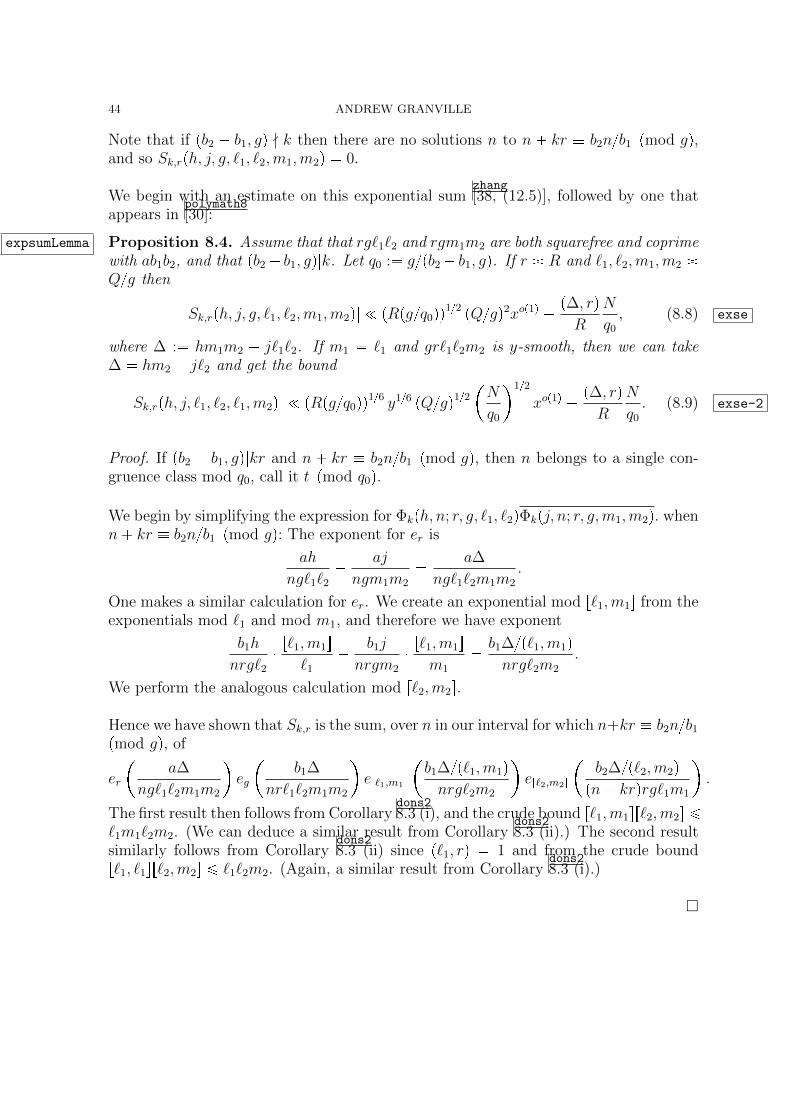
44 ANDREW GRANVILLE
Note that if pb2 b1, gq - k then there are no solutions n to n kr b2nb1 pmod gq,and so Sk,rph, j, g, `1, `2,m1,m2q 0.
We begin with an estimate on this exponential sumzhang[38, (12.5)], followed by one that
appears inpolymath8[30]:
expsumLemma Proposition 8.4. Assume that that rg`1`2 and rgm1m2 are both squarefree and coprimewith ab1b2, and that pb2 b1, gq|k. Let q0 : gpb2 b1, gq. If r R and `1, `2,m1,m2 Qg then
|Sk,rph, j, g, `1, `2,m1,m2q| ! pRpgq0qq12 pQgq2xop1q p∆, rqR
N
q0
, (8.8) exse
where ∆ : hm1m2 j`1`2. If m1 `1 and gr`1`2m2 is y-smooth, then we can take∆ hm2 j`2 and get the bound
|Sk,rph, j, `1, `2, `1,m2q| ! pRpgq0qq16 y16 pQgq12N
q0
12xop1q p∆, rq
R
N
q0
. (8.9) exse-2
Proof. If pb2 b1, gq|kr and n kr b2nb1 pmod gq, then n belongs to a single con-gruence class mod q0, call it t pmod q0q.
We begin by simplifying the expression for Φkph, n; r, g, `1, `2qΦkpj, n; r, g,m1,m2q. whenn kr b2nb1 pmod gq: The exponent for er is
ah
ng`1`2
aj
ngm1m2
a∆
ng`1`2m1m2
.
One makes a similar calculation for er. We create an exponential mod r`1,m1s from theexponentials mod `1 and mod m1, and therefore we have exponent
b1h
nrg`2
r`1,m1s`1
b1j
nrgm2
r`1,m1sm1
b1∆p`1,m1qnrg`2m2
.
We perform the analogous calculation mod r`2,m2s.
Hence we have shown that Sk,r is the sum, over n in our interval for which nkr b2nb1
pmod gq, of
er
a∆
ng`1`2m1m2
eg
b1∆
nr`1`2m1m2
er`1,m1s
b1∆p`1,m1qnrg`2m2
er`2,m2s
b2∆p`2,m2q
pn krqrg`1m1
.
The first result then follows from Corollarydons28.3 (i), and the crude bound r`1,m1sr`2,m2s ¤
`1m1`2m2. (We can deduce a similar result from Corollarydons28.3 (ii).) The second result
similarly follows from Corollarydons28.3 (ii) since p`1, rq 1 and from the crude bound
r`1, `1sr`2,m2s ¤ `1`2m2. (Again, a similar result from Corollarydons28.3 (i).)

BOUNDED GAPS BETWEEN PRIMES 45
9. The Grand Finaletypei-ii-sec
Our goal is to establish TheoremReducedRange6.1:
TheoremReducedRange6.1 Fix constants η, δ, A ¡ 0. Suppose that we have two sequences of complex
numbers αm, M m ¤ 2M , and βn, N n ¤ 2N , where βn satisfies the Siegel-Walfiszcondition, and that α β satisfies the necessary sieving condition, where x13 ! N ¤M ! x23, with x MN . Suppose also that Npyxεq R ¤ Nxε and x12plog xqB QR ¤ x12η, where y : xδ. For any A ¡ 0, for any integers a, b, b1 with ppabb1q ¡ y,we have
¸qPrQ,2Qs
D0 ppqq¤P pqq¤y
¸rPrR,2Rs,P prq¤y
qr squarefree
¸
na pmod rqnb pmod qq
pα βqpnq ¸
na pmod rqnb1 pmod qq
pα βqpnq
!A αβ x12
plog xqA ,
(9.1) straw-2
where D0 xε log log x. In fact it suffices to take 162η 90δ 1.
We chose r to be slightly less than N to ensure that the constraint n a pmod rq stillincorporates some non-trivial averaging in the α weight, which allows one to profitablyuse the dispersion method of Linnik. We chose q to be free of small prime factors, sothat two such q’s are likely to be coprime.
Throughout the argument below, the restrictions on m,n, q, r from the hypothesis willbe taken as given.
In the left-hand side of (straw-29.1) we replace the absolute value in the pq, rq term by a
complex number cq,r of absolute value 1, and then each pα βqp`q °mn` αpmqβpnq
to obtain, after a little re-arranging:
¸r
¸m
αpmq¸
q
¸n: mna pmod rq
cq,rβpnqp1mnb pmod qq 1mnb1 pmod qqq .
By the Cauchy-Schwarz inequality the square of this is
¤¸r
¸m
|αpmq|2 ¤ Rα2
times
¸r
¸m
¸q
¸n: mna pmod rq
cq,rβpnqp1mnb pmod qq 1mnb1 pmod qqq2
. (9.2) sq

46 ANDREW GRANVILLE
When we expand the sum, we obtain the sum of four terms of the form
¸r
¸m
¸q1,q2
¸n1,n2
mn1mn2a pmod rq
cq1,rcq2,rβpn1qβpn2q1mn1b1 pmod q1q1mn2b2 pmod q2q
¸r
¸q1,q2
¸n1,n2
n1n2 pmod rq
cq1,rcq2,rβpn1qβpn2q ¸m
1mb1n1 pmod q1qmb2n2 pmod q2qman1 pmod rq
where we get “” when b1 b2 b or b1, and “” otherwise, since pmn, qrq 1.Notice that the last sum is 0 unless b1n1 b2n2 pmod pq1, q2qq; and that this criterionis irrelevant if pq1, q2q 1.
9.1. The main terms. When the last sum (over m) is non-zero then we “expect” itto be Mrrq1, q2s. In our range this can be 1, which makes no sense for an individualsum, but we expect this to be about right “on average”. The key idea is to deal with thedeviation from this average using exponential sums. This is the “dispersion method”.First though, let us deal with the “expected” main term:
¸r
¸q1,q2
¸n1,n2
n2n1 pmod rqn2pb2b1qn1 pmod pq1,q2qq
cq1,rcq2,rβpn1qβpn2q M
rrq1, q2s .
We pull out the term with pq1, q2q 1 to obtain
¸r
¸q1,q2
pq1,q2q1
¸n1,n2
n1n2 pmod rq
cq1,rcq2,rβpn1qβpn2q M
rq1q2
,
which is independent of the values of b1, b2 and hence cancels, when we sum over thefour terms.
Otherwise g : pq1, q2q ¥ D0. If g ¤ NR then there are approximately NgR valuesof n2 for each n1. Hence by Cauchy-Schwarz¸
n1,n2
n2n1 pmod rqn2pb2b1qn1 pmod gq
|βpn1qβpn2q| ! N
gRβ2
Therefore the total contribution above is
!¸r
¸D0 g¤NR
¸q1,q2
g|q1, g|q2
N
gRβ2 gM
rq1q2
! xβ2
R
¸D0 g¤NR
1
g2! xβ2
RD0
.
For larger g, the sum above becomes
!¸r
¸NR g¤Q
¸n1,n2
n2n1 pmod rqn2pb2b1qn1 pmod gq
|βpn1qβpn2q| Mrg
Since there is at most one value of n2 for each n1 we can use Cauchy-Schwarz to showthat the sum over n1, n2 is ¤ β2. So the total contribution is β2M log x, which is

BOUNDED GAPS BETWEEN PRIMES 47
far smaller then the previous contribution, as M ¤ x1εR, by hypothesis. Hence thecontribution of the expected main terms is in total
Rα2 xβ2
RD0
12! αβ x12
plog xqA .
9.2. Crude error terms for large g. If g ¡ G : Q2RM then Mrrq1, q2s ¥ 1, andthe count of the number of m values is as above with an error term of Op1q. We willsimply sum up these crude error terms. (In fact one can take this error term for any g).Now if we Cauchy the sum over β we get in total ! p N
Rg 1qβ2. The sums over the
qi’s divisible by g, contribute Qg each, and the sum over r, contributes R, so over allg ¥ G the error term is
!¸
G g¤QRQ2
g2p NRg
1qβ2 ! Q2p NG2
R
Gqβ2.
Taking G Q2RM this is
! x
D2 1 xβ2
N! xplog xq2Bβ2
N
where D QR.15 Hence the contribution here is
! αβx12plog xqBpRNq12which is certainly acceptable given our choice of R.
9.3. Exponential sums. After removing these contributions, we are left with fourterms, each of which is bounded by a sum of the form
¸rR
¸g¤G
¸`1,`2Qgp`1,`2q1
¸
n1,n2Nn1n2 pmod rq
b1n1b2n2 pmod gq
βpn1qβpn2q
¸
mMmm0pn1,n2q pmod rg`1`2q
1 M
rg`1`2
writing q1 g`1, q2 g`2, where m0 m0pn1, n2q is that residue class mod g`1`2rwhich is b1n1 pmod g`1q, b2n2 pmod g`2q, an1 pmod rq. Using (
ExponExpan8.3) this is
!¸rR
¸g¤G
¸`1,`2Qgp`1,`2q1
¸0¤i¤J
Hi:2jGg
1
Hi
¸1¤|h|¤Hi
¸
n1,n2Nn1n2 pmod rq
n2pb2b1qn1 pmod gq
βpn1qβpn2qerg`1`2pm0pn1, n2qhq
.
Writing n1 n and n2 n kr for some k, |k| ¤ NR, this equals
!¸g¤G
¸0¤i¤J
Hi:2iGg
¸rR
¸`1,`2Qgp`1,`2q1
15We can divide G by pNRq12plog xqC , and still have a good error term.

48 ANDREW GRANVILLE
1
Hi
¸1¤|h|¤Hi
¸
k¤NRpb2b1,gq|k
¸nN
pb2b1qnb1kr pmod gq
βpnqβpn krqΦkph, n; r, g, `1, `2q
. (9.3) Esum
bearing in mind the definition (phi-def8.6), so that there is only a term if pb2 b1, gq|k .
We will see two techniques for dealing with these sums, both of which begin by usingthe Cauchy-Schwarz inequality to eliminate the βpnq factors, so reducing things toincomplete exponential sum estimates, which we handle by using the estimates fromSection
incompsec8.
9.4. Technique # 1. We replace the absolute value above by a complex number ch,`1,`2of absolute value 1, so that the sum
¸`1,`2Qgp`1,`2q1
1
Hi
¸1¤|h|¤Hi
¸n
βpnqβpn krqΦkph, n; r, g, `1, `2q
equals ¸nN
pb2b1qnb1kr pmod gq
βpnqβpn krq¸
`1,`2Qgp`1,`2q1
1
Hi
¸1¤|h|¤Hi
ch,`1,`2Φkph, n; r, g, `1, `2q. (9.4) PreCauchy
Applying the Cauchy-Schwarz inequality, the square of this is less than or equal to16¸n
|βpnqβpn krq|2 ¤¸n
|βpnq|4 β44
(applying the Cauchy-Schwarz inequality again), times
¸n
¸
`1,`2Qgp`1,`2q1
1
Hi
¸1¤|h|¤Hi
ch,`1,`2Φkph, n; r, g, `1, `2q
2
¤ 1
H2i
¸1¤|h|,|j|¤Hi
¸`1,`2,m1,m2Qgp`1,`2qpm1,m2q1
|Sk,rph, j, g, `1, `2,m1,m2q| ,
by expanding and then taking absolute values for each fixed h, j, `1, `2,m1,m2, wherethe exponential sum Sk,rph, j, `1, `2,m1,m2q is defined in (
S-def8.7). By Proposition
expsumLemma8.4(i),
this is xop1q times
! pRpb2 b1, gqq12 pQgq6NR
pb2 b1, gqg
1
H2i
¸1¤|h|,|j|¤Hi
¸`1,`2,m1,m2Qgp`1,`2qpm1,m2q1
phm1m2j`1`2, rq.
Now, in the sums in the second term let u hm1m2, v j`1`2 so that 1 ¤ |u|, |v| !HipQgq2 and the pair is represented at most τ3puqτ3pvq xop1q times. Therefore the
16If we apply Holder’s inequality with exponents 6, 6, 6, 2, we can replace β44 in this upper boundby pNg1q13β46; and more generally pNg1q12mβ42m, where g1 gpb2 b1, gq.

BOUNDED GAPS BETWEEN PRIMES 49
difference w u v satisifies |w| ! HipQgq2 is represented at most xop1qHipQgq2times. Now ¸
|w|¤Wpw, rq ¤
¸|w|¤W
¸d|pw,rq
d ¤¸d|rd
2W
d 1
¤ p2W rqτprq.
Hence the above is xop1q times
! pRpb2 b1, gqq12 pQgq6 N
R
pb2 b1, gqg
pQgq2ppQgq2 RHiq.
Collecting this information together, and summing over r and k, yields an upper boundon (
Esum9.3) of
! β24Nx
op1q ¸g¤G
¸0¤i¤J
R14Q3
g3pb2 b1, gq34 N12Q2
R121
g52pb2 b1, gq12 pMNq12R12
1
gpb2 b1, gq121
2i2
! β24Nx
op1qR14Q3 N12Q2
R12 pMNq12R12
Finally we assume that β2
4N12 ! β2
2xop1q (note that β2
2 ¤ β24N
12 by Cauchying),and therefore the total contribution is
! α2β2xop1qN12 pQRq3
R74 NpQRq2R32 R12N12x12
! α2β2xop1qx323η
N54 x74pδεq x12η
N12 x32pδεq Nx
12 1
2ε
(9.5) FinalBound1
using the inequalities Nxδε R ¤ Nxε, x12op1q ¤ QR ¤ x12η. Now sinceN ! x12, the last term is ! x1ε2. We will bound (
FinalBound19.5) in section
FinalSection9.6.
We remark that had we used PropositionexpsumLemma8.4(ii) in place of Proposition
expsumLemma8.4(i), then the
first term in (FinalBound19.5) would have been
x76 7
3η 7
4δ 5
4εN12 in place of x
323η 7
4pδεqN54.
This yields a suitable bound in a wider range for N , but not for all N " x13 so, eitherway, we need another argument for smaller N .
9.5. Technique # 2. We also employ a variation on this theme, including `1 in theoutside summation in (
PreCauchy9.4) when we apply Cauchy-Schwarz. Hence the square of our
quantity is
! Q
gβ4
4
1
H2i
¸1¤|h|,|j|¤Hi
¸`1Qg
¸`2,m2Qgp`2m2,`1q1
|Sk,rph, j, g, `1, `2, `1,m2q|.
By PropositionexpsumLemma8.4(ii), and the assumption that β2
4N12 ! β2
2xop1q,
! β4xop1q
pRyq16Q92
N12pb2 b1, gq23
g5 Q2
R
pb2 b1, gqg3
1
H2i
¸1¤|h|,|j|¤Hi
¸`2,m2Qg
phm2 j`2, rq

50 ANDREW GRANVILLE
Proceeding as above, and since τpuqτpvqτprq xop1q, we obtain
! β4xop1qpRyq16Q
92
N12pb2 b1, gq23
g5 Q2
R
pb2 b1, gqg3
Q2
g2 M
2iQ
as Hi 2iRQ2gM .
Collecting this information together, and summing over r and k, yields an upper boundon (
Esum9.3) of
! β2Nxop1q¸g¤G
¸0¤i¤J
pRyq112Q
94
N14 Q2
R12 pMQq122i2R12
1
g32pb2 b1, gq12
! β2Nxop1qpRyq112Q
94
N14 Q2
R12 pMQq12R12
.
Therefore the total contribution is
! α2β2xop1qy112pQRq94N34
R76 NpQRq2R32 N12pMNQRq12
.
! α2β2xop1qx
98 9
4η 5
4δ 7
6ε
N512 x12η 3
2pδεq
N12 N12x34 1
2η
.
using the inequalities Nxδε R ¤ Nxε, x12op1q ¤ QR ¤ x12η,
! α2β2xop1qx
7172 9
4η 5
4δ 7
6ε x
562η 3
2pδεq N12x
34 1
2η. (9.6) FinalBound2
as N " x13. The third term is ! x1ε2 provided N ¤ x12ηε.
We remark that had we used PropositionexpsumLemma8.4(i) in place of Proposition
expsumLemma8.4(ii), then the
first term above would have been
x118 11
4η 3
2δ 3
2εN in place of x
98 9
4η 5
4δ 7
6εN512.
This yields a suitable bound only for N somewhat bigger than x38, not for all N " x13,whereas the argument we have used allows N to be this small.
FinalSection
9.6. Bounds in different ranges. In (FinalBound19.5) and (
FinalBound29.6), we want the quantity in brackets
to be ! x1ε. We use (FinalBound19.5) in the range x
12ηε N ! x
12 , so that it is
! x78 17
4η 17
4ε 7
4δ x
34 5
2η 5
2ε 3
2δ x1ε2.
We use (FinalBound29.6) in the range x
13 ! N ¤ x
12η2ε, so that it is
! x7172 9
4η 5
4δ 7
6ε x
562η 3
2pδεq x1ε2.
These are all ! x1ε2, for a sufficiently small choice of ε ¡ 0, as long as
162η 90δ 1.CorrectNorms
9.7. Correcting the norms. We made some unnecessary assumption of the normsin the arguments above. In fact we used 4-norms and 8-norms. Simply using theinequalities, for γ supported in rM, 2M s, that γ2 ¤ γ4M
14 ¤ γ8M38, we can
correct TheoremReducedRange6.1 by replacing αβx12 by α8β8x
78.

BOUNDED GAPS BETWEEN PRIMES 51
9.8. Better results. Inpolymath8[30] the authors obtain better results using somewhat deeper
techniques.
One key observation is that y-smoothness was used in the above argument to constructa divisor r of a given integer d in a prespecified interval of multiplicative length y. Infact one can make do just with this property and, to improve our exponential sumestimates, that r also has a divisor in a prespecified interval of multiplicative length y.By going to such a larger class of moduli q they improve the restriction to
84η 48δ 1.
Following Zhang they also gained bounds on certain higher order convolutions (of theshape α 1 1 1), though here needing some deeper exponential sum estimates, andwere then able to improve the restriction to (slightly better than)
43η 27δ 1.

52 ANDREW GRANVILLE
10. Weaker hypotheses
In sectionexp-sec7 we stated that we only need the estimate (
pqp7.5) for the exponential sums in
(needExpSums7.4). It is worth noting (
pqp7.5) may be weakened to the upper bound ! pθ, for any given
θ P p12, 2
3q, and we can still obtain the same result:
From Propositioninc8.1 onwards we replace the exponent 1
2by θ, and 1
6by θ
2p1θq . Even-
tually this leads us in technique # 1, to replacing the first term in (FinalBound19.5) and the line
above, by
N12 pQRq22θ
R32θ1
¤ x1θp22θqηp 32θ1qpδεq
Np3θ1q
2
which is, for N ¡ x12ηε,
! x3θ4 57θ
2ηp 3
2θ1qδp3θ 3
2qε.
Similarly, in technique # 2, we replace the first term in (FinalBound29.6) and the line above, by
N34yθ
4p1θqpQRq2 3θ
4p1θq
R1 θ2p1θq
¤ xp23θ
4p1θqqp 1
2ηqp1 3θ
4p1θqqδp1 θ
2p1θqqε
N14 θ
2p1θq
which is x1ε, for N ¡ x13 , provided
p11θ 8qη p7θ 4qδ 2 3θ
6
so we deduce such a theorem provided θ 23.

BOUNDED GAPS BETWEEN PRIMES 53
References
[1] E. Bombieri, On the large sieve, Mathematika 12 (1965), 201–225.[2] E. Bombieri, H. Davenport Small difference between prime numbers, Proc. Roy. Soc. Ser. A 293
(1966), 1-18.[3] E. Bombieri, J. Friedlander, H. IwaniecPrimes in arithmetic progressions to large moduli, Acta
Math. 156 (1986), no. 3-4, 203–251.[4] E. Bombieri, J. Friedlander, H. Iwaniec, Primes in arithmetic progressions to large moduli. II,
Math. Ann. 277 (1987), no. 3, 361–393.[5] E. Bombieri, J. Friedlander, H. Iwaniec, Primes in arithmetic progressions to large moduli. III, J.
Amer. Math. Soc. 2 (1989), no. 2, 215–224.[6] T. Cochrane, C. Pinner, Using Stepanov’s method for exponential sums involving rational func-
tions, J. Number Theory 116 (2006), no. 2, 270–292.
[7] P. Deligne, La conjecture de Weil. II, Publications Mathematiques de l’IHES 52 (1980), 137–252.[8] P. D. T. A. Elliott, H. Halberstam, A conjecture in prime number theory, Symp. Math. 4 (1968),
59–72.[9] E. Fouvry, A new form of the error term in the linear sieve, Acta Arith., 37 (1980), 307–320.
[10] E. Fouvry, Autour du theoreme de Bombieri-Vinogradov, Acta Math. 152 (1984), no. 3-4, 219–244.[11] E. Fouvry, H. Iwaniec, On a theorem of Bombieri-Vinogradov type, Mathematika 27 (1980), no.
2, 135–152 (1981).[12] E. Fouvry, H. Iwaniec, Primes in arithmetic progressions, Acta Arith. 42 (1983), no. 2, 197–218.[13] J. Friedlander, A. Granville, Limitations to the equi-distribution of primes. I, Ann. of Math. 129
(1989), 363-382.[14] J. Friedlander, H. Iwaniec, Incomplete Kloosterman sums and a divisor problem, With an appendix
by Bryan J. Birch and Enrico Bombieri. Ann. of Math. (2) 121 (1985), no. 2, 319–350.[15] D. Goldston, J. Pintz, C. Yıldırım, Primes in tuples. I, Ann. of Math. 170 (2009), no. 2, 819–862.[16] D. Goldston, S. Graham, J. Pintz, C. Yıldırım, Small gaps between primes or almost primes,
Trans. Amer. Math. Soc. 361 (2009), no. 10, 5285–5330.[17] S. W. Graham, C. J. Ringrose, Lower bounds for least quadratic nonresidues, Analytic number
theory (Allerton Park, IL, 1989), 269–309, Progr. Math., 85, Birkhauser Boston, Boston, MA,1990.
[18] A. Granville, K. Soundararajan, Multiplicative number theory; the pretentious approach, to appear.[19] G. H. Hardy, J. E. Littlewood, Some problems of “Partitio Numerorum”, III: On the expression
of a number as a sum of primes, Acta Math. 44 (1923), 1–70.[20] D. R. Heath-Brown, Prime numbers in short intervals and a generalized Vaughan identity, Canad.
J. Math. 34 (1982), no. 6, 1365–1377.[21] H. A. Helfgott, Major arcs for Goldbach’s theorem, to appear.[22] D. Hensley, I. Richards, On the incompatibility of two conjectures concerning primes, Analytic
number theory (Proc. Sympos. Pure Math., Vol. XXIV, St. Louis Univ., St. Louis, Mo., 1972),pp. 123–127. Amer. Math. Soc., Providence, R.I., 1973.
[23] D. Hensley, I. Richards, Primes in intervals, Acta Arith. 25 (1973/74), 375–391.[24] H. D. Kloosterman, On the representation of numbers in the form ax2 by2 cz2 dt2, Acta
Mathematica 49 (1926), pp. 407–464.[25] H. Maier, Small differences between prime numbers, Michigan Math. J. 35 (1988), 323344.[26] J. Maynard, Bounded length intervals containing two primes and an almost-prime II, preprint.[27] L. J. Mordell, On a sum analogous to a Gauss’s sum, Quart. J. Math. Oxford Ser. 3 (1932),
161–167.[28] Y. Motohashi, J. Pintz, A smoothed GPY sieve, Bull. Lond. Math. Soc. 40 (2008), no. 2, 298–310.[29] J. Pintz, Polignac Numbers, Conjectures of Erdos on Gaps between Primes, Arithmetic Progres-
sions in Primes, and the Bounded Gap Conjecture, preprint.[30] D.H.J. Polymath, A new bound for small gaps between primes, preprint.[31] A. Schinzel, Remarks on the paper “Sur certaines hypotheses concernant les nombres premiers”,
Acta Arith. 7 (1961/1962) 1–8.
54 ANDREW GRANVILLE
[32] A. Selberg, On elementary methods in prime number-theory and their limitations, in Proc. 11thScand. Math. Cong. Trondheim (1949), Collected Works, Vol. I, 388397, Springer-Verlag, Berlin-Gottingen-Heidelberg, 1989.
[33] P. Shiu, A Brun-Titchmarsh theorem for multiplicative functions, J. Reine Angew. Math.313(1980), 161–170.
[34] K. Soundararajan, Small gaps between prime numbers: the work of Goldston-Pintz-Yildirim, Bull.Amer. Math. Soc. (N.S.) 44 (2007), no. 1, 1–18.
[35] R. C. Vaughan, Sommes trigonometriques sur les nombres premiers, C. R. Acad. Sci. Paris Ser.A 285 (1977), 981–983.
[36] A. I. Vinogradov, The density hypothesis for Dirichlet L-series, Izv. Akad. Nauk SSSR Ser. Mat.29 (1965), 903–934.
[37] A. Weil, Numbers of solutions of equations in finite fields, Bulletin of the American MathematicalSociety 55 (1949), 497–508.
[38] Y. Zhang, Bounded gaps between primes, to appear, Annals of Mathematics.
Departement de mathematiques et de statistiques, Universite de Montreal, MontrealQC H3C 3J7, Canada.
E-mail address: [email protected]


