
BUILDING REGULARITY FOR SIMPLIFIED MODELLING
EQC Project No. 06/514
by
Gregory MacRae and Bruce DeamDepartment of Civil and Natural Resources Engineering
University of CanterburyChristchurch 8140
New Zealand
June 2009
EQC Contact:Patricia Cheung
The Earthquake CommissionLevel 20
Majestic Centre100 Willis Street
Wellington
University of Canterbury Budget Number E5201

CONTENTS
Layman’s Abstract
Chapter 1. Introduction
Chapter 2. Mass Irregularity
Chapter 3. Stiffness-Strength Irregularity (Uniform Storey Height)
Chapter 4. Stiffness-Strength Irregularity (Variable Storey Height)
Chapter 5. Torsional Irregularity in Single Storey Structures
Chapter 6. Design for Torsional Irregularity.
Chapter 7. Diaphragm Flexibility
Chapter 8. Summary of Recommendations
Chapter 9. Opportunities for Further Work


LAYMAN’S ABSTRACT
As part of structural design, members in buildings are selected and detailed such that the expected demands, such as forces or displacements, on a structure are less than the capacity of the structure to resist those forces and displacements. However, to obtain these forces or displacements, structural analysis is required considering the loading applied to the building from its weight, its use, and other factors such as wind, or shaking of the ground in the case of earthquake, which is considered in this report.
Many different analysis methods are available for earthquake. Some give a realistic understanding of the behaviour of a structure in a particular earthquake, but are too complex for design. Many simple structures in New Zealand are designed using the NZ Structural Design code Equivalent Static Procedure. This procedure was developed for structures which have relatively regular configurations. For those structures with discontinuities, significant changes in stiffness, strength and mass over the height, or structures which have irregular plans or flexible diaphragms, it is possible that the Equivalent Static Procedure may underestimate the actual demands, which will result in unsafe structures. For this reason design codes have limitations on the amount of irregularity of structures designed according to the Equivalent Static Procedure. These limitations are based on engineering judgement, rather than on quantitative analysis, and it is not clear how much the demands are likely to change with different amounts of irregularity.
This project was initiated to quantify the effect of different degrees of irregularity on structures designed for earthquake using simplified analysis. The types of irregularity considered were:
(a) Vertical Irregularity i) Mass
ii) Stiffness -Strength(b) Horizontal (Plan) Irregularity
i) Torsionalii) Diaphragm
Code compliant structures expected to exhibit sensitivity to these types of analysis were selected. These were chosen so that they could represent a number of frame types. Simplified modelling was used in the analyses, so that many analyses could be conducted in a relatively short time. The structures were designed according to NZS1170.5 for regions of high, medium and low seismicity firstly as regular structures, and then they were redesigned as irregular structures. By subjecting the structures to a suite of records which represented design level shaking, the differences between the actual and predicted responses could be compared for structures with different levels of irregularity.
Relationships between the degree of irregularity and the change in behaviour could therefore be developed which allows guidance as to:
a) when the effect of structural irregularity can be ignored, and b) the change in demands for different degrees of structural irregularity.

The key findings in the study are:
A simple method was developed to quantify irregularity, based on the engineering demand parameter of interstorey drift, was more robust than that used in previous literature.
Relationships were developed to describe the change in response as a function of mass irregularity.
For stiffness and strength irregularity, relationships between stiffness and strength were developed for realistic structures. Only these realistic relationships were considered when evaluating stiffness and strength irregularity for a constant storey height. Relationships to describe the change in response as a function of stiffness-strength irregularity were developed.
A second type of stiffness-strength irregularity can occur due to changes in interstorey height. Relationships to describe the change in response as a function of stiffness-strength irregularity were developed.
It was shown that torsional effects resulting from earthquake shaking can be modelled well using impulsive loading. The rotational mass inertia effect is significant with systems with very little rotational restraint, but not for systems with significant torsional restraint. A relationship for the amount of torsional restraint required for a specified amount of torsional response was described which can be used in simplified analysis.
It was shown that diaphragm flexibility is unlikely to increase the lateral forces in most structures due to the increase in period, and the decrease in spectral acceleration. However, structural displacement may increase as a result of the increase in spectral displacement. Conservative methods to assess the likely increase in displacement were developed.
While this study has developed some simple tools for structural engineers to assess how building irregularity is likely to affect the design process, its most significant contributions to decreasing structural damage during an earthquake are:
Helping designers qualitatively understand how irregularity affects building performance so they can mitigate its effects during the preliminary design stage.
Providing a rigorous technical basis for revision of the regularity provisions in the Structural Actions Standard, NZS 1170.5.
Providing a basis for defining acceptable irregularity limitations for structures.
The funding provided by the Earthquake Commission for this work was used primarily to support Vinod Kota Sadashiva during his doctoral research at the University of Canterbury. Additional work was carried out by others. In particular, Eu Ving Au studied torsional effects in structures as part of his undergraduate research project in 2007. Matt Spooner undertook an undergraduate project at the University of Canterbury in 2008 related to floor flexibility. Other students and staff also contributed to this work.

CHAPTER 1. INTRODUCTION
CHAPTER 1. INTRODUCTION
There have been significant advances in both modelling software and computing power since most modern seismic design codes were first drafted. However, even with these advances, full inelastic dynamic time-history analysis of 3-D structural models that include diaphragm flexibility, statistical variations in element behaviour, etc. are currently not conducted for the majority of structures in New Zealand. Simple analysis methods and simple models will be used for some time yet.
New Zealand engineers need conceptually simple methods:i) for design of full structuresii) to enable a rapid check of likely building performanceiii) for preliminary sizing of members before some more sophisticated studies are
undertaken.
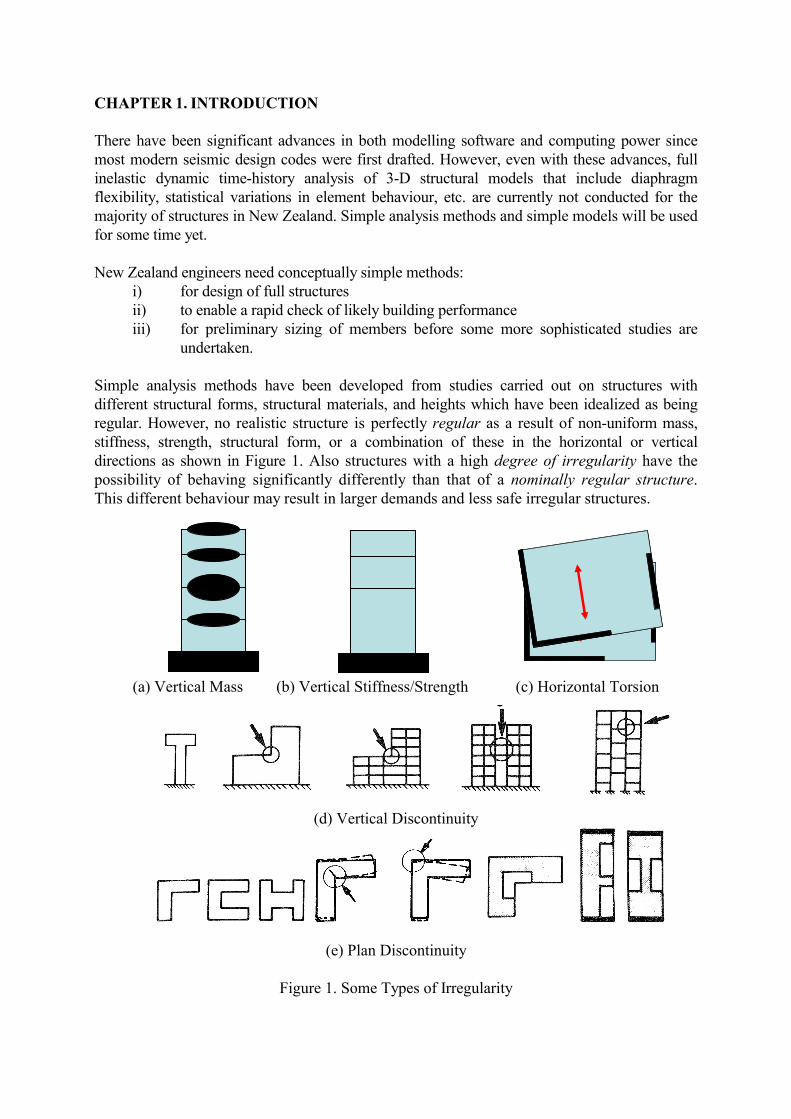
Simple analysis methods have been developed from studies carried out on structures with different structural forms, structural materials, and heights which have been idealized as being regular. However, no realistic structure is perfectly regular as a result of non-uniform mass, stiffness, strength, structural form, or a combination of these in the horizontal or vertical directions as shown in Figure 1. Also structures with a high degree of irregularity have the possibility of behaving significantly differently than that of a nominally regular structure. This different behaviour may result in larger demands and less safe irregular structures.
(a) Vertical Mass (b) Vertical Stiffness/Strength (c) Horizontal Torsion
(d) Vertical Discontinuity
(e) Plan Discontinuity
Figure 1. Some Types of Irregularity

In order to prevent possible undesirable behaviour due to irregularity, limits on the amount of allowable irregularity have been developed. These limits were developed by consensus, rather than being based on quantitative data. Similar limits are used in codes around the world. For example, the SEAOC blue book states that:
“.. irregularities create great uncertainties in the ability of the structure to meet the design objectives of [the code] … These Requirements are intended onlyto make designers aware of the existence and potential detrimental effects of irregularities, and to provide minimum requirements for their accommodation….”, (C104.5.3, SEAOC 1999),
and
“Extensive engineering experience and judgment are required to quantify irregularities and provide guidance for special analysis. As yet, there is no complete prescription for … irregularities”. (C104.5.1 SEAOC 1999).
Studies have not been conducted particularly to quantify the variation in response associated with a particular degree of irregularity so the validity of the irregularity limits, or the variation in response due to structures meeting these limits, is not known.
There is therefore a need to address this issue. This project seeks to develop rational criteria for irregularity based on the change in response for a particular level of irregularity. The particular types of irregularity considered include:
a) Vertical Mass Irregularity b) Vertical Stiffness-Strength Irregularity for structures with constant interstorey heightsc) Vertical Stiffness-Strength Irregularity for structures with different interstorey heightsd) Horizontal stiffness or strength irregularity on rigid floor diaphragm structures which
cause torsional deformations e) Horizontal floor diaphragm flexibility which affects the structural behaviour
The report is laid out primarily in terms of papers, as these have been written as the work has progresses. The journal papers associated with the different topic areas are listed below. Conference papers and posters have also been written related to some of these topics. These are generally referenced in the journal papers.
Chapter 2. Mass Irregularity
Paper: Sadashiva V. K., MacRae G. A., Deam B., Determination of Structural Irregularity Limits – Mass Irregularity Example, Submitted to the Bulletin of the NZ Society of Earthquake Engineering, March 2009.
Chapter 3. Stiffness-Strength Irregularity (Uniform Storey Height)
Paper: Sadashiva V. K., MacRae G. A., Deam B., Seismic Response of Structures with Coupled Vertical Stiffness-Strength Irregularities, To be submitted to the Bulletin of the NZ Society of Earthquake Engineering.
Chapter 4. Stiffness-Strength Irregularity (Variable Storey Height)Paper: Sadashiva V. K., MacRae G. A., Deam B., Effects of Coupled Vertical
Stiffness-Strength Irregularities due to Modified Interstorey Height, To be submitted to the Bulletin of the NZ Society of Earthquake Engineering.
Chapter 5. Torsional Irregularity in Single Storey Structures
Paper: Au E. V., MacRae G. A, Pettinga D., Deam B. and Sadashiva V., Torsionally Irregular Single Story Structure Seismic Response, Submitted to the Bulletin of the NZ Society of Earthquake Engineering, February 2009. Accepted pending minor changes.
Chapter 6. Design for Torsional Irregularity
Chapter 7. Diaphragm Flexibility
Paper: Spooner M., Deam B., MacRae G. A., Sadashiva V. and Gardiner D., Flexible Floor Diaphragm Seismic Response, To be submitted to the Bulletin of the NZ Society of Earthquake Engineering.
Chapter 8. Summary of Recommendations
Chapter 9. Opportunities for Further Work

CHAPTER 2. MASS IRREGULARITY

1
DETERMINATION OF STRUCTURAL IRREGULARITY LIMITS – MASS IRREGULARITY EXAMPLE
Vinod K. Sadashiva1, Gregory A. MacRae2 & Bruce L. Deam3
SUMMARY
Structures may be irregular due to non-uniform distributions of mass, stiffness, strength or due to their structural form. For regular structures, simple analysis techniques such as the Equivalent Static (ES) Method, have been calibrated against sophisticated analysis methods, such as Inelastic Dynamic Time-History Analysis (IDTHA). Most worldwide codes allow simple analysis technique to be used only for structures which satisfy regularity limits. Currently, such limits are based on engineering judgement and lack proper calibration. This paper describes a simple and efficient method for quantifying irregularity limits of 3, 5, 9 and 15 storey shear type structures, assumed to be located in Wellington, Christchurch and Auckland. They were designed in accordance with the Equivalent Static Method of NZS 1170.5. Regular structures were defined to have constant mass at every floor level and were either designed to produce constant interstorey drift ratio at all the floors simultaneously or to cause uniform stiffness distribution throughout the elevation of structure. Design structural ductility factors of 1, 2, 4 and 6, and target (design) interstorey drift ratios ranging between 0.5% and 3% were used in this study. Inelastic dynamic time-history analysis was carried out by subjecting these structures to code design level earthquake records. Irregular structures were created by adding additional floor mass of 1.5, 2.5, 3.5 and 5 times the regular floor mass at the first level, mid-height and the roof, and they were designed similar to regular structures.
It was found that additional mass, when applied at the first floor or roof generally, produced higher drift demands than regular structures for all mass ratios. When the mass ratio was present at the mid-height, the structures generally tended to produce lesser drift demands than the corresponding regular structures. A simple equation was defined to give a conservative measure of increase in interstorey drift response due to mass irregularity which can be used to set irregularity limits.
1 PhD Candidate, Dept. of Civil and Natural Resources Engineering, University of Canterbury, 2 Associate Professor, Dept. of Civil and Natural Resources Engineering, University of Canterbury, 3 Leicester Steven EQC Lecturer, Dept. of Civil and Natural Resources Engineering, University of Canterbury, Christchurch, New Zealand.
INTRODUCTION
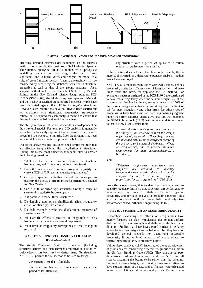
Current earthquake codes define structural configuration as either regular or irregular in terms of size and shape of the building, arrangement of the structural and non-structural elements within the structure, distribution of mass in the building etc. A regular structure can be envisaged to have uniformly distributed mass, stiffness, strength and structural form. When one or more of these properties is non-uniformly distributed, either individually or in combination with other properties in any direction the structure is referred to as being irregular. Structural irregularity may occur for many reasons. For example, a factory with heavy machinery or an educational institution with a library level at one level that leads to irregular distribution of mass as shown in Figure 1(a), a residential building having a car park in the basement producing a flexible first storey as shown in Figure 1(b), a
shopping complex with setbacks to accommodate boundary offset requirements as shown in the plan of Figure 1(c), buildings with flexible, rigid or no diaphragms at a floor level, structural plan having different lateral load resisting systems (resulting in torsion) as shown in the plan of Figure 1(d). These types of irregularities and many other types of irregularities as given in current worldwide design documents are classified as architecturally planned (AP) irregularities.
A structure can also be irregular because of unplanned effects which are referred to as aleatoric uncertainties (AU). These include deliberate and accidental rearrangement of loadings, as well as material strength and stiffness variations.
For the above reasons, structures are never perfectly regular and hence designers routinely need to evaluate the degree of irregularity and therefore the demands that this places on the structure during an earthquake.
BULLETIN OF THE NEW ZEALAND SOCIETY FOR EARTHQUAKE ENGINEERING, Vol. XX, No. Y, Month 2009
2
Structural demand estimates are dependent on the analysis method. For example, the most costly 3-D Inelastic Dynamic Time-History Analysis (IDTHA) method with appropriate modelling, can consider most irregularities, but it takes significant time to build, verify and analyse the model to a suite of ground motion records. Aleatory uncertainties may be considered by modelling the statistical variation in structural properties as well as that of the ground motions. Also, analysis method such as the Equivalent Static (ES) Method, defined in the New Zealand seismic design standard NZS 1170.5 (SNZ 2004); the Modal Response Spectrum Method; and the Pushover Method are simplified methods which have been calibrated against the IDTHA for regular structures. However, such calibrations have not always been carried out for structures with significant irregularity. Appropriate calibration is required for each analysis method to ensure that they estimate a realistic value of likely demand.
The ability to estimate structural demands is also dependent on the structural model. For example, 2-D analysis is generally not able to adequately represent the response of significantly irregular 3-D structures. Similarly, floor diaphragms may need to be modelled to adequately represent the behaviour.
Due to the above reasons, designers need simple methods that are effective in quantifying the irregularities in structures. Having this as the focal objective, this paper aims to answer the following questions:
1. What are the current recommendations for structural irregularities, and from where do they come from?
2. Does the past research on mass irregularity justify the current NZS 1170.5 mass irregularity requirements?
3. Can a simple and effective method be developed to quantify the effects of irregularities for structures designed for New Zealand?
4. Can a suite of shear-type structures having a range of structural irregularity be developed?
5. Is it possible to model these structures? 6. Do damping assumptions significantly affect irregularity
effects on shear-type structures? 7. Do code methods predict the displacement response of
structures well? 8. What are the effects of position and magnitude of mass
irregularity on the actual structural responses? 9. What level of irregularity corresponds to what change in
response?
NZS 1170.5 CURRENT CONSIDERATION FOR IRREGULARITY
The simple Equivalent Static (ES) method (including structural actions and displacement amplification due to P-Delta effects) has been used to design many NZ structures. NZS 1170.5 permits the ES method to be used to design:
any structure less than 10m high;
any structure having a fundamental translational period of less than 0.4s;
any structure with a period of up to 2s if certain regularity requirements are satisfied.
If the structure does not meet the above requirements, then a more sophisticated, and therefore expensive analysis, method needs to be employed.
NZS 1170.5, similar to many other worldwide codes, defines irregularity limits for different types of irregularities, and these limits form the basis for applying the ES method. For example, structures designed using NZS 1170.5 are considered to have mass irregularity when the seismic weight, Wi, of the structure and live loading in any storey is more than 150% of the seismic weight of either adjacent storey. Such a limit of 1.5 for mass irregularity and other limits for other types of irregularities have been specified from engineering judgment rather than from rigorous quantitative analysis. For example, the SEAOC blue book (1999), with recommendations similar to that in NZS 1170.5, states that:
“.. irregularities create great uncertainties in the ability of the structure to meet the design objectives of [the code] … These Requirements are intended only to make designers aware of the existence and potential detrimental effects of irregularities, and to provide minimum requirements for their accommodation….”, (C104.5.3),
and
“Extensive engineering experience and judgment are required to quantify irregularities and provide guidance for special analysis. As yet, there is no complete prescription for … irregularities” (C104.5.1).
From the above quotes, it is evident that there is a need to quantify regularity limits so that structures can be designed to have a consistent level of reliability for each type of irregularity and for each analysis or modelling method. This aim is consistent with a probabilistic multi-objective performance based earthquake engineering (PBEE).
PREVIOUS RESEARCH ON MASS IRREGULARITY
Researchers evaluating the effects of irregularities have mainly focussed on plan irregularities due to non-uniform distribution of mass, strength and stiffness in the horizontal direction. Studies that have investigated vertical irregularity effects have given insight into the behaviour but they have not developed general methods for quantifying acceptable irregularity limits. A brief summary of works related to vertical mass irregularity is presented below. Valmundsson and Nau (1997) investigated the appropriateness of provisions for considering different irregularities as laid in the Uniform Building Code (UBC). They considered two-dimensional building frames with heights of 5, 10 and 20 storeys, assuming the beams to be stiffer than the columns. For each structure height, uniform structures were defined to have constant mass of 35 Mg, and stiffnesses were calculated to give a set of 6 desired fundamental periods. The maximum
Heavy Floor Level
Flexible Storey
Lateral Load Resisting System
Rigid Diaphragm Flexible Diaphragm
Figure 1: Examples of Vertical and Horizontal Structural Irregularities
(a) (b) (c) (d)
Duct

3
calculated drifts from the lateral design forces for the regular structures having the target period were found to lie within the UBC limit. Mass irregularities at three locations in the elevation of structures were then applied by means of mass ratios (ratio of modified mass of irregular case to the mass of uniform structure at a floor level) ranging between 0.1 and 5, and responses were calculated for design ductility’s of 1, 2, 6, and 10 considering four earthquake records. The increase in ductility demand was found to be not greater than 20% for a mass ratio of 1.5 and mass discontinuity was most critical when located on lower floors. Mass irregularity was found to be least important of the irregularity effects.
Al-Ali and Krawinkler (1998) assessed the effects of vertical irregularities by evaluating roof drift demands and the distribution of storey demands over the height of the structure, obtained by conducting elastic and inelastic dynamic analyses on two-dimensional single-bay 10-storey generic structures, assuming a column hinge model. A base structure was defined to have a uniform distribution of mass over the height and an associated stiffness distribution that resulted in a straight-line first mode shape with storey stiffnesses tuned to produce a first mode period of 3s when designed according to modal superposition technique. Cases with mass irregularities were created by changing the mass distribution of the base model and keeping the same stiffness distribution as the base model. Mass ratios between 0.25 and 4 were chosen and applied either at one floor or in series of floors, and stiffness distribution was tuned until the structures had a fundamental period of 3s. Dynamic analyses were then conducted on each structure by subjecting them to a suite of 15 ground motion records without considering P-Delta effects and utilising Rayleigh damping to obtain a damping ratio of 5% for the first and fourth modes. It was found that mass irregularities showed relatively small effects on elastic and inelastic storey shear and storey drift demands. It was also shown that mass increase at the top had a relatively larger effect on roof and storey drifts than when additional mass was applied at mid-height or at the lower floors. Again it was concluded that mass irregularity effects were the least compared to other types of vertical irregularities.
Michalis et. al (2006) carried out incremental dynamic analyses on a realistic LA9 nine storey steel frame to evaluate the effect of irregularities for each performance level, from serviceability to global collapse. A mass ratio of 2 was applied at series of locations over the selected frame and effects of mass irregularity were evaluated. It was found that the influence of mass irregularity on interstorey drifts was comparable to the influence of stiffness irregularity.
Although the above researchers and few others (e.g Chintanapakdee and Chopra (2004), Tremblay and Poncet (2005)) have given useful insights into the topic of vertical irregularities and their effects on structural response, these studies are not carried out with a design perspective. It may be seen that in many of the cases described above an “apples-to-apples” comparison was not conducted. That is, regular and irregular structures were not generally designed for the same engineering demand parameter (EDP). For example, irregular structures were sometimes designed to have the same period as the regular structures. This is problematic because it is possible that the design drifts of the irregular structure with the same period may be significantly different from that of the regular structure. They may even violate the code drift requirements. Furthermore, the structure with the greater design drift would be expected to have greater drift demands in the dynamic analysis. It would be better if both regular and irregular structures are designed to the same EDP (e.g. drift) so that a valid comparison may be made. Earlier studies are also limited to specific structural type/height and there is a lack of information on the appropriateness of the limit of 150% imposed on mass irregularity. Also, the above studies
may not be relevant for structures designed according to NZ code analysis procedures which have some differences from overseas methods.
SIMPLE METHODOLOGY FOR EVALUATING VERTICAL IRREGULARITY EFFECTS
Recognising the need to provide rational basis for the structural irregularity limits and to have a consistent meaningful comparison between regular and irregular structures designed according to NZ code, the following simple methodology is proposed:
1. Define an engineering demand parameter that characterises structural damage. Peak interstorey drift ratio over all the storeys has been used as the engineering demand parameter (EDP) to assess the vertical irregularity effects in this paper.
2. Choose a set of interstorey drift capacities that span the range of values that could be used by designers (e.g. from 0.5% to 3%). Then for each target interstorey drift capacity and degree of irregularity: a. Design a regular structure using the Equivalent Static
method to the target interstorey drift capacity. b. Introduce the desired irregularity into the structure and
use the Equivalent Static method to design this new structure to the same target interstorey drift. The mass irregularity considered here is most easily quantified as the ratio of the floor mass in this new structure to the corresponding floor mass of the regular structure.
c. Evaluate the maximum interstorey drift for both structures using IDTHA for a suite of design ground motions.
d. Evaluate the performance for all of the ground motion records either a) as the difference between the median responses of the two structures or b) as the probability that the demand for the irregular building is greater than the demand for the regular building.
3. The performance distributions for the chosen degrees of irregularity and target interstorey drift ratio may then be used to characterise the effect of both of these variables and select appropriate limits.
STRUCTURAL FORMS CONSIDERED & DEFINITION OF REGULAR STRUCTURES
The above methodology was applied to simple design models representing 3, 5, 9 and 15 storey shear type of structures. Such a simple model that is adequate for determination of overall structural response (Cruz and Chopra, 1986) was adopted to aid carry out a parametric study and reduce computational effort.
There is no specification for the distributions of stiffness and strength within structures designed using the NZS 1170.5 ES method. Two classes of building having constant floor mass at every floor level were therefore chosen to represent the two extremes of design choice for stiffness that defined the base (regular) structures. It is expected that the configuration of realistic frames would fall between these two extreme design models and hence the results serve as upper and lower bounds. One class of building was designed for all storeys to have a constant interstorey drift ratio (labelled as CISDR) and the other class was designed for all storeys to have constant stiffness (labelled CS) with the target interstorey drift ratio at the first storey. To achieve this task, storey stiffness’s were iterated until the critical storey/storeys had the design (target) interstorey drift ratio (DISDR). These two models and their deflection profiles are shown in Figure 2. For the CISDR model, at the end of iteration a constant strength to stiffness ratio is established at each floor level, so the shear strength provided at each level was the minimum required to resist the
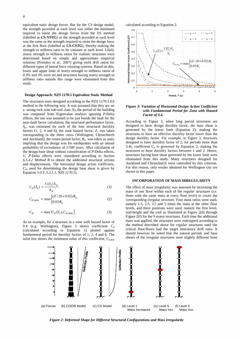
4
equivalent static design forces. But for the CS design model, the strength provided at each level was either the minimum required to resist the design forces from the ES method (labelled as CS-VSTG) or the strength provided at each level was the same as the strength required to resist the design force at the first floor (labelled as CS-CSTG), thereby making the strength to stiffness ratio to be constant at each level. Likely storey strength to stiffness ratios for realistic structures were determined based on simple and approximate empirical relations (Priestley et al., 2007) giving yield drift ratios for different types of lateral force resisting systems. Based on this, lower and upper limit of storey strength to stiffness ratios of 0.3% and 3% were set and structures having storey strength to stiffness ratio outside this range were eliminated from this study.
Design Approach: NZS 1170.5 Equivalent Static Method
The structures were designed according to the NZS 1170.5 ES method in the following way. It was assumed that they are on a strong rock (site sub-soil class A), the period of the building was computed from Eigenvalue analysis ignoring P-Delta effects, the site was assumed to be just beside the fault for the near-fault factor calculation, the structural performance factor, Sp, was estimated for each of the four structural ductility factors (1, 2, 4 and 6), the zone hazard factor, Z, was taken corresponding to the three cities (Wellington, Christchurch and Auckland), the return period factor, Ru, was taken as unity implying that the design was for earthquakes with an annual probability of exceedance of 1/500 years. After calculation of the design base shear without consideration of P-Delta effects, V, P-Delta effects were considered according to Section 6.5.4.2 Method B to obtain the additional structural actions and displacements. The horizontal design action coefficient, Cd, used for determining the design base shear is given by Equation 3 (Cl. 5.2.1.1, NZS 1170.5).
µkSTC
TC pd
)()( 1
1 = (1)
⎩⎨⎧ +
=u
ud R
RZC
03.0)02.020/(
maxmin, (2)
}{ min,1),(max ddd CTCC = (3)
As an example, for a structure in a zone with hazard factor of 0.4 (e.g. Wellington), Figure 3 shows coefficient Cd (calculated according to Equation 1) plotted against fundamental period for ductility factors of 1, 2, 4 and 6. The solid line shows the minimum value of this coefficient, Cd,min
calculated according to Equation 2.
0
0.1
0.2
0.3
0.4
0.5
0.6
0.7
0.8
0 1 2 3 4 5
Period, T (s)
Hor
izon
tal D
esig
n A
ctio
n C
oeffi
cien
t, Cd(
T)
µ = 1 µ = 2
µ = 4 µ = 6
Figure 3: Variation of Horizontal Design Action Coefficient with Fundamental Period for Zone with Hazard Factor of 0.4.
According to Figure 3, when long period structures are designed to have design ductility factor, the base shear is governed by the lower limit (Equation 2), making the structures to have an effective ductility factor lower than the design ductility factor. For example, in Figure 3, structures designed to have ductility factor of 2, for periods more than 3.4s, coefficient Cd is governed by Equation 2, making the structures to have ductility factors between 1 and 2. Hence, structures having base shear governed by the lower limit were eliminated from this study. Many structures designed for Auckland and Christchurch were controlled by this criterion. For this reason, only results obtained for Wellington city are shown in this paper.
INCORPORATION OF MASS IRREGULARITY
The effect of mass irregularity was assessed by increasing the mass of one floor within each of the regular structures (i.e. those with the same mass at every floor level) to create the corresponding irregular structure. Four mass ratios were used, namely 1.5, 2.5, 3.5 and 5 times the mass at the other floor levels, and three positions were used, namely the first level, mid-height and the roof as illustrated in Figure 2(d) through Figure 2(f) for the 9 storey structures. Each time the additional mass was applied, the structures were redesigned according to the method described above for regular structures until the critical floor/floors had the target interstorey drift ratio. It should however be noted that the natural periods and base shears of the irregular structures were slightly different from
⎩⎨⎧ +
=u
ud R
RZC
03.0)02.020/(
maxmin,
µkSTC
TC pd
)()( 1
1 =
Def
lect
ion
Pro
file
Def
lect
ion
Pro
file
Def
lect
ion
Pro
file
Def
lect
ion
Pro
file
Def
lect
ion
Pro
file
Def
lect
ion
Pro
file
(a) Forces (b) CISDR Model (c) CS Model (d) Level 1 (e) Level 5 (f) Level 9 Mass Increased Mass Incr. Mass Incr.
Figure 2: Deformed Shape for Different Structural Configurations and Mass Irregularity

5
those of the regular structures because their stiffness distribution was adjusted to produce the same interstorey drift as the corresponding CISDR and CS regular structures.
STRUCTURAL MODELLING AND ANALYSIS
To investigate the effects of structural modelling on interstorey drift demands, each frame was modelled in two ways. Frames were initially modelled as a vertical shear beam, assuming that the columns develop a point of contraflexure at mid-height of each storey under the earthquake loading (Tagawa et al. 2004). Secondly, each frame was modelled as a combination of vertical shear beam and a vertical flexural beam (representing all of the continuous columns in the structure) that is pinned at the base. This model is labelled as SFB and is shown in Figure 4.
∆n
∆2
∆1
∆n-1
Rigid Link
Pin
Shear-Beam Flexural-Beam
∆n
∆2
∆1
∆n-1
Rigid Link
Pin
Shear-Beam Flexural-Beam
Figure 4: Combined Vertical Shear and Flexural Beam (SFB model)
Previous studies (MacRae et al. 2004, Tagawa et al. 2006) have shown that SFB model can represent real structural behaviour well and magnitude of interstorey drift demands are decreased with the inclusion of this vertical flexural beam, which is desirable. A parameter defined as continuous column stiffness ratio cci, (MacRae et al. 2004), representing the stiffness of flexural-beam relative to the shear beam at the ith floor level is computed using Equation 4.
oii
icci
KHIE
3=α (4)
where cci = continuous column stiffness ratio at level, i;
E = elastic modulus;
Ii = moment of inertia at the ith level;
Hi = storey height of the ith level; and
Koi = lateral initial stiffness of the ith level.
It is shown (Tagawa 2005) that when parameter cci = 0, the structure behaves like a shear structure in which each storey behaves as an independent single-degree-of-freedom (SDOF) system. For structures with low post-elastic stiffness, this can result in large interstorey drift concentrations due to soft storey mechanisms. Tagawa has also showed that for real frames, cc varies between 0.25 and 1.58 and the variation in response between these values was small. Hence, for this study a continuous column stiffness ratio at any level of 0.5 was assumed and the additional moment of inertia at each level was calculated according to Equation 4.
Selection and Scaling of Earthquake Ground Motions for Time-History Analysis
Recent work by Baker (2007) has shown that random ground motion record selection can produce unrealistic scaling and
increase the scatter of the absolute responses. Baker also suggests that records matching the shape of the uniform hazard spectrum may incorrectly evaluate the response at different periods. It is expected that the record selection and scaling will have less influence on the relative responses used in this study than on the absolute responses. Hence, the 20 SAC (SEAOC-ATC-CUREE) earthquake ground motion records (tabulated in Table 1) for Los Angeles, with probabilities of exceedance of 10% in 50 years, were used for the ground motion suite. Response spectra were developed for each of the selected records and the accelerations within each record were scaled so that its single-degree-of-freedom elastic displacement response spectrum matched the design interstorey drift for NZS 1170.5 in the city chosen. Here, both the structural ductility factor and structural performance factor were unity.
Table 1: Ground Motion Suite used for Time-History Analysis.
SAC Name Earthquake Record Moment
MagnitudePGA (g)
LA01 Imperial Valley, 1940, El Centro 6.9 0.461
LA02 Imperial Valley, 1940, El Centro 6.9 0.676
LA03 Imperial Valley, 1979, Array #05 6.5 0.393
LA04 Imperial Valley, 1979, Array #05 6.5 0.488
LA05 Imperial Valley, 1979, Array #06 6.5 0.301
LA06 Imperial Valley, 1979, Array #06 6.5 0.234
LA07 Landers, 1992, Barstow 7.3 0.421
LA08 Landers, 1992, Barstow 7.3 0.426
LA09 Landers, 1992, Yermo 7.3 0.52
LA10 Landers, 1992, Yermo 7.3 0.360
LA11 Loma Prieta, 1989, Gilroy 7 0.665
LA12 Loma Prieta, 1989, Gilroy 7 0.970
LA13 Northridge, 1994, Newhall 6.7 0.678
LA14 Northridge, 1994, Newhall 6.7 0.657
LA15 Northridge, 1994, Rinaldi RS 6.7 0.533
LA16 Northridge, 1994, Rinaldi RS 6.7 0.580
LA17 Northridge, 1994, Sylmar 6.7 0.570
LA18 Northridge, 1994, Sylmar 6.7 0.817
LA19 North Palm Springs, 1986 6 1.02
LA20 North Palm Springs, 1986 6 0.987
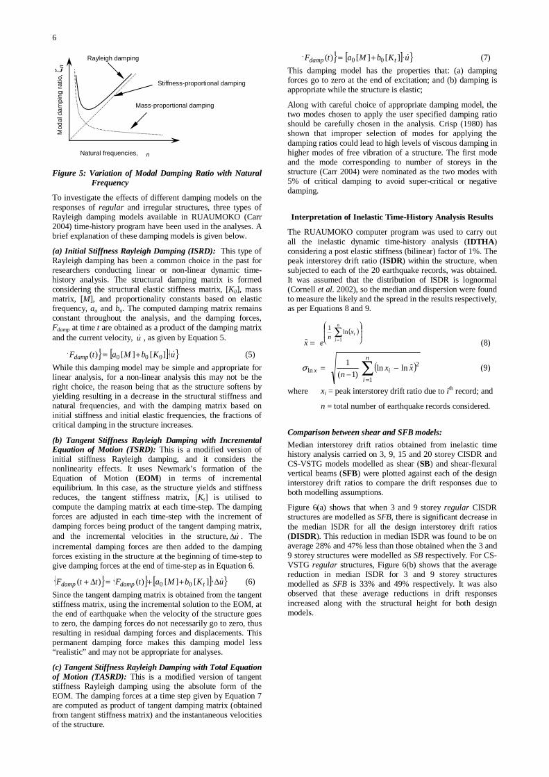
Choice of Damping Model for Time-History Analysis
A common damping model available in most of the time-history programs (e.g., SAP 2000, ETABS, RUAUMOKO etc.) for linear and non-linear analysis of multi-degree-of-freedom (MDOF) systems is the Rayleigh damping model. As shown in Figure 5, this type of damping model has structural damping matrix, [C], given as the summation of mass and stiffness proportional damping models, where the mass damping matrix is given as the product of the proportionality constant, a and the mass matrix, [M], and the stiffness damping matrix is given as the product of proportionality constant, b and the stiffness matrix, [K].
6
Figure 5: Variation of Modal Damping Ratio with Natural Frequency
To investigate the effects of different damping models on the responses of regular and irregular structures, three types of Rayleigh damping models available in RUAUMOKO (Carr 2004) time-history program have been used in the analyses. A brief explanation of these damping models is given below.
(a) Initial Stiffness Rayleigh Damping (ISRD): This type of Rayleigh damping has been a common choice in the past for researchers conducting linear or non-linear dynamic time-history analysis. The structural damping matrix is formed considering the structural elastic stiffness matrix, [K0], mass matrix, [M], and proportionality constants based on elastic frequency, ao and bo. The computed damping matrix remains constant throughout the analysis, and the damping forces, Fdamp at time t are obtained as a product of the damping matrix and the current velocity, u , as given by Equation 5.
{ } [ ]{ }uKbMatFdamp ][][)( 000 += (5) While this damping model may be simple and appropriate for linear analysis, for a non-linear analysis this may not be the right choice, the reason being that as the structure softens by yielding resulting in a decrease in the structural stiffness and natural frequencies, and with the damping matrix based on initial stiffness and initial elastic frequencies, the fractions of critical damping in the structure increases.
(b) Tangent Stiffness Rayleigh Damping with Incremental Equation of Motion (TSRD): This is a modified version of initial stiffness Rayleigh damping, and it considers the nonlinearity effects. It uses Newmark’s formation of the Equation of Motion (EOM) in terms of incremental equilibrium. In this case, as the structure yields and stiffness reduces, the tangent stiffness matrix, [Kt] is utilised to compute the damping matrix at each time-step. The damping forces are adjusted in each time-step with the increment of damping forces being product of the tangent damping matrix, and the incremental velocities in the structure, u∆ . The incremental damping forces are then added to the damping forces existing in the structure at the beginning of time-step to give damping forces at the end of time-step as in Equation 6.
{ } { } [ ]{ }uKbMatFttF tdampdamp ∆++=∆+ ][][)()( 00 (6) Since the tangent damping matrix is obtained from the tangent stiffness matrix, using the incremental solution to the EOM, at the end of earthquake when the velocity of the structure goes to zero, the damping forces do not necessarily go to zero, thus resulting in residual damping forces and displacements. This permanent damping force makes this damping model less “realistic” and may not be appropriate for analyses.
(c) Tangent Stiffness Rayleigh Damping with Total Equation of Motion (TASRD): This is a modified version of tangent stiffness Rayleigh damping using the absolute form of the EOM. The damping forces at a time step given by Equation 7 are computed as product of tangent damping matrix (obtained from tangent stiffness matrix) and the instantaneous velocities of the structure.
{ } [ ]{ }uKbMatF tdamp ][][)( 00 += (7) This damping model has the properties that: (a) damping forces go to zero at the end of excitation; and (b) damping is appropriate while the structure is elastic;
Along with careful choice of appropriate damping model, the two modes chosen to apply the user specified damping ratio should be carefully chosen in the analysis. Crisp (1980) has shown that improper selection of modes for applying the damping ratios could lead to high levels of viscous damping in higher modes of free vibration of a structure. The first mode and the mode corresponding to number of storeys in the structure (Carr 2004) were nominated as the two modes with 5% of critical damping to avoid super-critical or negative damping.
Interpretation of Inelastic Time-History Analysis Results
The RUAUMOKO computer program was used to carry out all the inelastic dynamic time-history analysis (IDTHA) considering a post elastic stiffness (bilinear) factor of 1%. The peak interstorey drift ratio (ISDR) within the structure, when subjected to each of the 20 earthquake records, was obtained. It was assumed that the distribution of ISDR is lognormal (Cornell et al. 2002), so the median and dispersion were found to measure the likely and the spread in the results respectively, as per Equations 8 and 9.
( )⎟⎟
⎠
⎞⎜⎜
⎝
⎛∑
==
n
iix
nex 1
ln1
ˆ (8)
( )∑=
−−
=n
iix xx
n1
2ln ˆlnln
)1(1σ (9)
where xi = peak interstorey drift ratio due to ith record; and
n = total number of earthquake records considered.
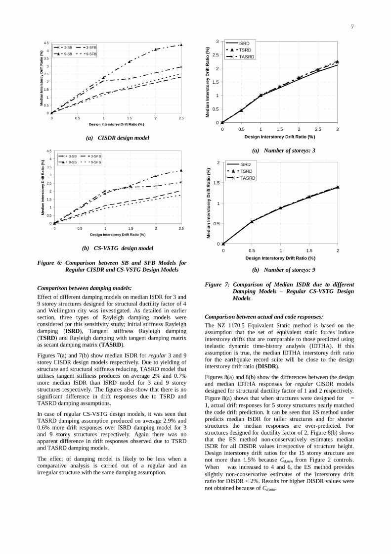
Comparison between shear and SFB models: Median interstorey drift ratios obtained from inelastic time history analysis carried on 3, 9, 15 and 20 storey CISDR and CS-VSTG models modelled as shear (SB) and shear-flexural vertical beams (SFB) were plotted against each of the design interstorey drift ratios to compare the drift responses due to both modelling assumptions.
Figure 6(a) shows that when 3 and 9 storey regular CISDR structures are modelled as SFB, there is significant decrease in the median ISDR for all the design interstorey drift ratios (DISDR). This reduction in median ISDR was found to be on average 28% and 47% less than those obtained when the 3 and 9 storey structures were modelled as SB respectively. For CS-VSTG regular structures, Figure 6(b) shows that the average reduction in median ISDR for 3 and 9 storey structures modelled as SFB is 33% and 49% respectively. It was also observed that these average reductions in drift responses increased along with the structural height for both design models.
Stiffness-proportional damping
Mass-proportional damping
Natural frequencies, n
Rayleigh damping M
odal
dam
ping
ratio
, ζn
7
0
0.5
1
1.5
2
2.5
3
3.5
4
4.5
0 0.5 1 1.5 2 2.5
Design Interstorey Drift Ratio (%)
Med
ian
Inte
rsto
rey
Drif
t Rat
io (%
)
3-SB 3-SFB
9-SB 9-SFB
(a) CISDR design model
0
0.5
1
1.5
2
2.5
3
3.5
4
4.5
0 0.5 1 1.5 2 2.5
Design Interstorey Drift Ratio (%)
Med
ian
Inte
rsto
rey
Drif
t Rat
io (%
)
3-SB 3-SFB
9-SB 9-SFB
(b) CS-VSTG design model
Figure 6: Comparison between SB and SFB Models for Regular CISDR and CS-VSTG Design Models
Comparison between damping models: Effect of different damping models on median ISDR for 3 and 9 storey structures designed for structural ductility factor of 4 and Wellington city was investigated. As detailed in earlier section, three types of Rayleigh damping models were considered for this sensitivity study; Initial stiffness Rayleigh damping (ISRD), Tangent stiffness Rayleigh damping (TSRD) and Rayleigh damping with tangent damping matrix as secant damping matrix (TASRD).
Figures 7(a) and 7(b) show median ISDR for regular 3 and 9 storey CISDR design models respectively. Due to yielding of structure and structural stiffness reducing, TASRD model that utilises tangent stiffness produces on average 2% and 0.7% more median ISDR than ISRD model for 3 and 9 storey structures respectively. The figures also show that there is no significant difference in drift responses due to TSRD and TASRD damping assumptions.
In case of regular CS-VSTG design models, it was seen that TASRD damping assumption produced on average 2.9% and 0.6% more drift responses over ISRD damping model for 3 and 9 storey structures respectively. Again there was no apparent difference in drift responses observed due to TSRD and TASRD damping models.
The effect of damping model is likely to be less when a comparative analysis is carried out of a regular and an irregular structure with the same damping assumption.
0
0.5
1
1.5
2
2.5
3
0 0.5 1 1.5 2 2.5 3
Design Interstorey Drift Ratio (%)
Med
ian
Inte
rsto
rey
Drif
t Rat
io (%
)
ISRDTSRDTASRD
(a) Number of storeys: 3
0
0.5
1
1.5
2
0 0.5 1 1.5 2
Design Interstorey Drift Ratio (%)
Med
ian
Inte
rsto
rey
Drif
t Rat
io (%
)
ISRDTSRDTASRD
(b) Number of storeys: 9
Figure 7: Comparison of Median ISDR due to different Damping Models – Regular CS-VSTG Design Models
Comparison between actual and code responses: The NZ 1170.5 Equivalent Static method is based on the assumption that the set of equivalent static forces induce interstorey drifts that are comparable to those predicted using inelastic dynamic time-history analysis (IDTHA). If this assumption is true, the median IDTHA interstorey drift ratio for the earthquake record suite will be close to the design interstorey drift ratio (DISDR).
Figures 8(a) and 8(b) show the differences between the design and median IDTHA responses for regular CISDR models designed for structural ductility factor of 1 and 2 respectively. Figure 8(a) shows that when structures were designed for = 1, actual drift responses for 5 storey structures nearly matched the code drift prediction. It can be seen that ES method under predicts median ISDR for taller structures and for shorter structures the median responses are over-predicted. For structures designed for ductility factor of 2, Figure 8(b) shows that the ES method non-conservatively estimates median ISDR for all DISDR values irrespective of structure height. Design interstorey drift ratios for the 15 storey structure are not more than 1.5% because Cd,min from Figure 2 controls. When was increased to 4 and 6, the ES method provides slightly non-conservative estimates of the interstorey drift ratio for DISDR < 2%. Results for higher DISDR values were not obtained because of Cd,min.

8
0
0.5
1
1.5
2
2.5
3
3.5
4
4.5
0 0.5 1 1.5 2 2.5 3
Design Interstorey Drift Ratio (%)
Med
ian
Inte
rsto
rey
Drif
t Rat
io (%
)3 Storey 5 Storey9 Storey 15 StoreyDISDR
(a) Structural Ductility Factor, = 1
0
0.5
1
1.5
2
2.5
3
3.5
4
4.5
0 0.5 1 1.5 2 2.5 3
Design Interstorey Drift Ratio (% )
Med
ian
Inte
rsto
rey
Drif
t Rat
io (%
)
3 Storey 5 Storey9 Storey 15 StoreyDISDR
(b) Structural Ductility Factor, = 2
Figure 8: Comparison between Actual and Code Response for Regular CISDR Models
For regular CS-VSTG structures designed for = 1, the ES method over-estimates median ISDR for all the DISDR considered in this study as shown in Figure 9(a). Figure 9(b) shows that for any structure height designed for = 2, the actual drift responses closely matched with the code prediction for DISDR < 1.5%. Again when was increased to 6, it was seen that code over-estimates drift response for DISDR > 1.5%.
0
0.5
1
1.5
2
2.5
3
0 0.5 1 1.5 2 2.5 3
Design Interstorey Drift Ratio (%)
Med
ian
Inte
rsto
rey
Drif
t Rat
io (%
)
3 Storey 5 Storey9 Storey 15 StoreyDISDR
(c) Structural Ductility Factor, = 1
0
0.5
1
1.5
2
2.5
3
0 0.5 1 1.5 2 2.5 3
Design Interstorey Drift Ratio (%)
Med
ian
Inte
rsto
rey
Drif
t Rat
io (%
)
3 Storey 5 Storey9 Storey 15 StoreyDISDR
(d) Structural Ductility Factor, = 2
Figure 9: Comparison between Actual and Code Response for Regular CS-VSTG Models
Effect of mass irregularity location and magnitude: 3, 5, 9 and 15 storey structures having mass irregularity were designed for three cities (Wellington, Christchurch and Auckland) considering four structural ductility factors (1, 2, 4 and 6). These shear type structures modelled as a combination of vertical shear and flexural beams were subjected to a suite of 20 earthquake records and by tangent stiffness Rayleigh damping based on the total equilibrium, and post-elastic stiffness factor of 1% inelastic time-history analysis were carried out to obtain peak interstorey drift responses. Median ISDR responses from irregular structures were then compared with those corresponding to regular structures to estimate the increase in drift demand for each of the design interstorey drift ratios (DISDR). To investigate the effectiveness of magnitude of additional masses used to define irregular structures, four mass ratios of 1.5, 2.5, 3.5 and 5 times the floor mass at corresponding floor level of regular structure were adopted in this study. To investigate the sensitivity of location of mass ratios on additional median ISDR response, the chosen mass ratios were added at first, mid-height and topmost level of all the structures chosen in this study.
For brevity, results for 3, 5, 9 storey structures designed for structural ductility factor of 2 are only presented in the following plots to show the effect of mass irregularity. The response plot labels in the following figures have the format “N-L(Q)”, where N refers to the number of storeys in the structure, L refers to the location (floor level) of the irregularity and Q defines the magnitude of irregularity (mass ratio).
Figure10 shows the effect of mass irregularity location and magnitude of mass ratio on median ISDR for CISDR design models. For all structure heights, the maximum increase in median ISDR due to mass ratio of 1.5 at the first and topmost level is less than 9% and 6% respectively. For many DISDR, it can be seen that regular structures produced slightly higher drift demands than when mass ratio of 1.5 was applied at mid-height storey of all structures. The maximum increase in median ISDR at this height, over the regular structure is found to be less than 2%. When the mass ratio was increased from 1.5 to a maximum of 5 at the three chosen positions, mass irregularity when present at either extreme floors tended to produce higher drift demands than regular structures and for taller structures it is seen that mass ratio at mid-height of structures always produced lesser median ISDR than those produced by regular structures. A maximum increase in
9
median ISDR of 20% and 25% was observed due to any mass ratio present at first and topmost floor respectively and this increase in response produced due to mass ratio at mid-height was less than 6%.
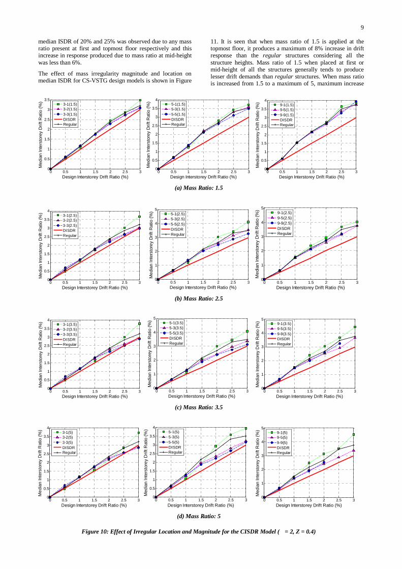
The effect of mass irregularity magnitude and location on median ISDR for CS-VSTG design models is shown in Figure
11. It is seen that when mass ratio of 1.5 is applied at the topmost floor, it produces a maximum of 8% increase in drift response than the regular structures considering all the structure heights. Mass ratio of 1.5 when placed at first or mid-height of all the structures generally tends to produce lesser drift demands than regular structures. When mass ratio is increased from 1.5 to a maximum of 5, maximum increase
0 0.5 1 1.5 2 2.5 30
0.5
1
1.5
2
2.5
3
3.5
Design Interstorey Drift Ratio (%)
Med
ian
Inte
rsto
rey
Drif
t Rat
io (%
) 3-1(1.5)3-2(1.5)3-3(1.5)DISDRRegular
0 0.5 1 1.5 2 2.5 3
0
0.5
1
1.5
2
2.5
3
3.5
4
Design Interstorey Drift Ratio (%)
Med
ian
Inte
rsto
rey
Drif
t Rat
io (%
) 5-1(1.5)5-3(1.5)5-5(1.5)DISDRRegular
0 0.5 1 1.5 2 2.5 3
0
0.5
1
1.5
2
2.5
3
3.5
4
Design Interstorey Drift Ratio (%)
Med
ian
Inte
rsto
rey
Drif
t Rat
io (%
) 9-1(1.5)9-5(1.5)9-9(1.5)DISDRRegular
(a) Mass Ratio: 1.5
0 0.5 1 1.5 2 2.5 30
0.5
1
1.5
2
2.5
3
3.5
4
Design Interstorey Drift Ratio (%)
Med
ian
Inte
rsto
rey
Drif
t Rat
io (%
) 3-1(2.5)3-2(2.5)3-3(2.5)DISDRRegular
0 0.5 1 1.5 2 2.5 3
0
1
2
3
4
5
Design Interstorey Drift Ratio (%)
Med
ian
Inte
rsto
rey
Drif
t Rat
io (%
) 5-1(2.5)5-3(2.5)5-5(2.5)DISDRRegular
0 0.5 1 1.5 2 2.5 3
0
1
2
3
4
5
Design Interstorey Drift Ratio (%)
Med
ian
Inte
rsto
rey
Drif
t Rat
io (%
) 9-1(2.5)9-5(2.5)9-9(2.5)DISDRRegular
(b) Mass Ratio: 2.5
0 0.5 1 1.5 2 2.5 30
0.5
1
1.5
2
2.5
3
3.5
4
Design Interstorey Drift Ratio (%)
Med
ian
Inte
rsto
rey
Drif
t Rat
io (%
) 3-1(3.5)3-2(3.5)3-3(3.5)DISDRRegular
0 0.5 1 1.5 2 2.5 3
0
1
2
3
4
5
Design Interstorey Drift Ratio (%)
Med
ian
Inte
rsto
rey
Drif
t Rat
io (%
) 5-1(3.5)5-3(3.5)5-5(3.5)DISDRRegular
0 0.5 1 1.5 2 2.5 3
0
1
2
3
4
5
Design Interstorey Drift Ratio (%)
Med
ian
Inte
rsto
rey
Drif
t Rat
io (%
) 9-1(3.5)9-5(3.5)9-9(3.5)DISDRRegular
(c) Mass Ratio: 3.5
0 0.5 1 1.5 2 2.5 30
0.5
1
1.5
2
2.5
3
3.5
4
Design Interstorey Drift Ratio (%)
Med
ian
Inte
rsto
rey
Drif
t Rat
io (%
) 3-1(5)3-2(5)3-3(5)DISDRRegular
0 0.5 1 1.5 2 2.5 3
0
0.5
1
1.5
2
2.5
3
3.5
4
Design Interstorey Drift Ratio (%)
Med
ian
Inte
rsto
rey
Drif
t Rat
io (%
) 5-1(5)5-3(5)5-5(5)DISDRRegular
0 0.5 1 1.5 2 2.5 3
0
1
2
3
4
5
Design Interstorey Drift Ratio (%)
Med
ian
Inte
rsto
rey
Drif
t Rat
io (%
) 9-1(5)9-5(5)9-9(5)DISDRRegular
(d) Mass Ratio: 5
Figure 10: Effect of Irregular Location and Magnitude for the CISDR Model ( = 2, Z = 0.4)

10
in median ISDR due to any mass ratio was found to be less than 6% and 19% for additional mass located at first or mid-height of structures, and 56% for mass ratio at topmost floor level. Again, generally for higher DISDR in many cases, when any additional mass was applied at first floor or mid-height,
drift responses decreased compared to corresponding regular structures.
Figure 12 shows the effect of mass ratio and its location on CS-CSTG model, designed for structural ductility factor of 2. For a mass ratio of 1.5, Figure 12 (a) shows that the maximum
0 0.5 1 1.5 2 2.5 30
0.5
1
1.5
2
2.5
3
Design Interstorey Drift Ratio (%)
Med
ian
Inte
rsto
rey
Drif
t Rat
io (%
) 3-1(1.5)3-2(1.5)3-3(1.5)DISDRRegular
0 0.5 1 1.5 2 2.5 3
0
0.5
1
1.5
2
2.5
3
Design Interstorey Drift Ratio (%)
Med
ian
Inte
rsto
rey
Drif
t Rat
io (%
)
5-1(1.5)5-3(1.5)5-5(1.5)DISDRRegular
0 0.5 1 1.5 2 2.5 3
0
0.5
1
1.5
2
2.5
3
Design Interstorey Drift Ratio (%)
Med
ian
Inte
rsto
rey
Drif
t Rat
io (%
) 9-1(1.5)9-5(1.5)9-9(1.5)DISDRRegular
(a) Mass Ratio: 1.5
0 0.5 1 1.5 2 2.5 30
0.5
1
1.5
2
2.5
3
Design Interstorey Drift Ratio (%)
Med
ian
Inte
rsto
rey
Drif
t Rat
io (%
)
3-1(2.5)3-2(2.5)3-3(2.5)DISDRRegular
0 0.5 1 1.5 2 2.5 3
0
0.5
1
1.5
2
2.5
3
Design Interstorey Drift Ratio (%)
Med
ian
Inte
rsto
rey
Drif
t Rat
io (%
)
5-1(2.5)5-3(2.5)5-5(2.5)DISDRRegular
0 0.5 1 1.5 2 2.5 30
0.5
1
1.5
2
2.5
3
Design Interstorey Drift Ratio (%)
Med
ian
Inte
rsto
rey
Drif
t Rat
io (%
) 9-1(2.5)9-5(2.5)9-9(2.5)DISDRRegular
(b) Mass Ratio: 2.5
0 0.5 1 1.5 2 2.5 30
0.5
1
1.5
2
2.5
3
Design Interstorey Drift Ratio (%)
Med
ian
Inte
rsto
rey
Drif
t Rat
io (%
)
3-1(3.5)3-2(3.5)3-3(3.5)DISDRRegular
0 0.5 1 1.5 2 2.5 3
0
0.5
1
1.5
2
2.5
3
Design Interstorey Drift Ratio (%)
Med
ian
Inte
rsto
rey
Drif
t Rat
io (%
)
5-1(3.5)5-3(3.5)5-5(3.5)DISDRRegular
0 0.5 1 1.5 2 2.5 30
0.5
1
1.5
2
2.5
3
Design Interstorey Drift Ratio (%)
Med
ian
Inte
rsto
rey
Drif
t Rat
io (%
)
9-1(3.5)9-5(3.5)9-9(3.5)DISDRRegular
(c) Mass Ratio: 3.5
0 0.5 1 1.5 2 2.5 30
0.5
1
1.5
2
2.5
3
Design Interstorey Drift Ratio (%)
Med
ian
Inte
rsto
rey
Drif
t Rat
io (%
) 3-1(5)3-2(5)3-3(5)DISDRRegular
0 0.5 1 1.5 2 2.5 3
0
0.5
1
1.5
2
2.5
3
Design Interstorey Drift Ratio (%)
Med
ian
Inte
rsto
rey
Drif
t Rat
io (%
) 5-1(5)5-3(5)5-5(5)DISDRRegular
0 0.5 1 1.5 2 2.5 3
0
0.5
1
1.5
2
2.5
3
Design Interstorey Drift Ratio (%)
Med
ian
Inte
rsto
rey
Drif
t Rat
io (%
) 9-1(5)9-5(5)9-9(5)DISDRRegular
(d) Mass Ratio: 5
Figure 11: Effect of Irregular Location and Magnitude for the CS-VSTG Model ( = 2, Z = 0.4)

11
increase in median ISDR for each structure height is produced when the additional mass is present at the topmost floor than first or mid-height level. When the mass ratio was increased to 5, the maximum increase in median ISDR is shown in Figure 12 (d) to be 40%, obtained from 3 storey structure having the additional mass at the roof. Figure 12 also shows that the
effect of mass irregularity decreases as the structure height increases, irrespective of magnitude of mass irregularity. It can also be seen that for many cases, the additional mass at the first floor tended to produce lesser median ISDR than the regular structure.
0 0.5 1 1.5 2 2.5 30
0.5
1
1.5
2
2.5
3
Design Interstorey Drift Ratio (%)
Med
ian
Inte
rsto
rey
Drif
t Rat
io (%
) 3-1(1.5)3-2(1.5)3-3(1.5)DISDRRegular
0 0.5 1 1.5 2 2.5 3
0
0.5
1
1.5
2
2.5
3
Design Interstorey Drift Ratio (%)
Med
ian
Inte
rsto
rey
Drif
t Rat
io (%
) 5-1(1.5)5-3(1.5)5-5(1.5)DISDRRegular
0 0.5 1 1.5 2 2.5 3
0
0.5
1
1.5
2
2.5
3
Design Interstorey Drift Ratio (%)
Med
ian
Inte
rsto
rey
Drif
t Rat
io (%
) 9-1(1.5)9-5(1.5)9-9(1.5)DISDRRegular
(a) Mass Ratio: 1.5
0 0.5 1 1.5 2 2.5 30
0.5
1
1.5
2
2.5
3
Design Interstorey Drift Ratio (%)
Med
ian
Inte
rsto
rey
Drif
t Rat
io (%
) 3-1(2.5)3-2(2.5)3-3(2.5)DISDRRegular
0 0.5 1 1.5 2 2.5 3
0
0.5
1
1.5
2
2.5
3
Design Interstorey Drift Ratio (%)
Med
ian
Inte
rsto
rey
Drif
t Rat
io (%
) 5-1(2.5)5-3(2.5)5-5(2.5)DISDRRegular
0 0.5 1 1.5 2 2.5 3
0
0.5
1
1.5
2
2.5
3
Design Interstorey Drift Ratio (%)
Med
ian
Inte
rsto
rey
Drif
t Rat
io (%
) 9-1(2.5)9-5(2.5)9-9(2.5)DISDRRegular
(b) Mass Ratio: 2.5
0 0.5 1 1.5 2 2.5 30
0.5
1
1.5
2
2.5
3
Design Interstorey Drift Ratio (%)
Med
ian
Inte
rsto
rey
Drif
t Rat
io (%
)
3-1(3.5)3-2(3.5)3-3(3.5)DISDRRegular
0 0.5 1 1.5 2 2.5 3
0
0.5
1
1.5
2
2.5
3
Design Interstorey Drift Ratio (%)
Med
ian
Inte
rsto
rey
Drif
t Rat
io (%
)
5-1(3.5)5-3(3.5)5-5(3.5)DISDRRegular
0 0.5 1 1.5 2 2.5 3
0
0.5
1
1.5
2
2.5
3
Design Interstorey Drift Ratio (%)
Med
ian
Inte
rsto
rey
Drif
t Rat
io (%
) 9-1(3.5)9-5(3.5)9-9(3.5)DISDRRegular
(c) Mass Ratio: 3.5
0 0.5 1 1.5 2 2.5 30
0.5
1
1.5
2
2.5
3
Design Interstorey Drift Ratio (%)
Med
ian
Inte
rsto
rey
Drif
t Rat
io (%
) 3-1(5)3-2(5)3-3(5)DISDRRegular
0 0.5 1 1.5 2 2.5 3
0
0.5
1
1.5
2
2.5
3
Design Interstorey Drift Ratio (%)
Med
ian
Inte
rsto
rey
Drif
t Rat
io (%
) 5-1(5)5-3(5)5-5(5)DISDRRegular
0 0.5 1 1.5 2 2.5 30
0.5
1
1.5
2
2.5
3
Design Interstorey Drift Ratio (%)
Med
ian
Inte
rsto
rey
Drif
t Rat
io (%
) 9-1(5)9-5(5)9-9(5)DISDRRegular
(d) Mass Ratio: 5
Figure 12: Effect of Irregular Location and Magnitude for the CS-CSTG Model ( = 2, Z = 0.4)

12
Determination of Irregularity Limit For each design model designed for a structural ductility factor, maximum median interstorey drift for each mass ratio was determined as:
Step 1. For each structure height with increased mass at the chosen irregularity position, compute the maximum increase in median ISDR from all DISDR;
Step 2. Repeat Step 1 for all the three positions chosen for applying additional mass;
Step 3. Compute the maximum of median ISDR’s obtained from Step 2;
Step 4. Repeat Step 3 for all the structural heights considered in this study;
Step 5. Compute the maximum of median ISDR’s obtained from Step 4;
Figure 13(b) shows the maximum median increase in ISDR due to irregularity (obtained from Step 5) plotted against mass ratios for structural ductility factor of 2. From Figure 11 through Figure 13, it can be seen that for all mass ratios at any chosen position, CISDR models produced higher median ISDR than CS models, but Figure 13(b) shows that structures having uniform stiffness distribution (CS model) produce higher increase in median ISDR (i.e. compared to regular structures) than when the same structures are designed to produce constant drift at every floor level (CISDR model). Also, for CISDR models, the increase in median ISDR almost varies linearly with mass ratio for all the structural ductility factors as shown in Figure 13(a) through 13(d).
Since real structures are assumed to have vertical structural configuration between CISDR and CS models, a simple equation given by Equation 10 is developed to estimate the increase in seismic demand due to irregularity for any structure.
)1(15 −= MRIRR (10) where IRR is the Irregular response greater than regular
response; and MR is the Mass ratio.
This equation is conservative due to the following reasons:
(a) The structures are assumed to be shear-type, assumed to be resting on soil class A and in a major city having highest zone hazard factor of 0.4 (Wellington), and designed in accordance with the ES method alone;
(b) Critical design model from all structural heights, considering the mass irregularity location that produced maximum increase in median ISDR was used to formulate the equation.
Equation 10 may be used to estimate the likely increase in response due to irregularity for design. For example, if it was decided that mass irregularity should produce less than 15% additional interstorey drift, then Figure14 shows that mass ratio needs to be less than 2. The figure also shows that the code value of 1.5 mass ratio corresponds to an increase in median ISDR of approximately 7.5% due to mass irregularity.
0
10
20
30
40
50
60
1 2 3 4 5 6Mass Ratio
Irreg
ular
resp
onse
gre
ater
than
R
egul
ar re
spon
se (%
)
CISDRCS-VSTGCS-CSTG
0
10
20
30
40
50
60
1 2 3 4 5 6Mass Ratio
Irreg
ular
resp
onse
gre
ater
than
R
egul
ar re
spon
se (%
)
CISDRCS-VSTGCS-CSTG
(a) Structural Ductility Factor, = 1 (b) Structural Ductility Factor, = 2
0
10
20
30
40
50
60
1 2 3 4 5 6Mass Ratio
Irreg
ular
resp
onse
gre
ater
than
R
egul
ar re
spon
se (%
)
CISDRCS-VSTGCS-CSTG
0
10
20
30
40
50
60
1 2 3 4 5 6Mass Ratio
Irreg
ular
resp
onse
gre
ater
than
R
egul
ar re
spon
se (%
)
CISDRCS-VSTGCS-CSTG
(c) Structural Ductility Factor, = 4 (d) Structural Ductility Factor, = 6
Figure 13: Increase in Median ISDR due to Mass Irregularities in Structures designed for different Structural Ductility Factors
IRR = 15 (MR – 1)
IRR = 15 (MR – 1)

13
0
10
20
30
40
50
60
1 2 3 4 5Mass Ratio
Irreg
ular
resp
onse
gre
ater
th
an R
egul
ar re
spon
se (%
)
Figure 14: Determination of Mass Irregularity Limit
CONCLUSIONS
The findings from this rigorous study on structural irregularity effects can be summarised as follows:
1. Current regularity provisions in NZS 1170.5 are based on overseas irregularity recommendations. They are based on engineering judgement and lack rational justification.
2. Past research on vertical irregularities effects does not justify the appropriateness of regularity limits slated in the NZS 1170.5. Better meaningful comparison is obtained if structures designed to produce a target drift are compared with the actual drift demand rather than tuning the structures to have the same period. Also, earlier works may not be appropriate for structures designed for NZ scenario;
3. A method to quantify vertical irregularity effects was proposed. This method was applied to evaluate the effects of mass irregularity on simple shear type structures of 3, 5, 9 and 15 storey heights, assumed to be located in Wellington, Christchurch and Auckland, and designed for a range of structural ductility factors;
4. Regular structures were defined to have constant floor mass at every floor level and using the NZ ES method, the structures were either designed to produce constant target interstorey drift ratio at all the floors simultaneously (CISDR) or to have uniform stiffness distribution throughout the elevation of structure making the first floor to have the target interstorey drift ratio (CS). While for CISDR model constant strength to stiffness ratios were established through design at all floor levels, for CS design the storey shear strengths were either provided as the minimum strength required to resist the design forces at every level (CS-VSTG) or a constant shear strength of magnitude equivalent to resist design force at the first level (CS-CSTG) was provided at all the floor levels. Mass irregular structures were created by introducing additional floor mass of magnitude of 1.5, 2.5, 3.5 and 5 times the regular floor mass and were applied at first level, mid-height and the roof before redesigning them similar to regular structures. All the structures were then analysed using inelastic dynamic time-history analysis to obtain the change in the median peak interstorey drift responses due to mass irregularity;
5. Regular and irregular structures modelled as a combination of vertical shear and flexural beam (SFB) have shown to represent the likely structural behaviour well compared to when the same structures were modelled as a vertical shear beam (SB) alone. The reduction in ISDR obtained due to SFB models was found to be as much as 50% over SB models;
6. Choice of the type of Rayleigh damping model for inelastic time-history analysis has shown to be not
significant for assessing irregularity effects since any variation in response occur in both regular and irregular structure analyses;
7. Median interstorey drift ratio estimates due to NZS 1170.5 Equivalent Static Method was found to be not always conservative;
8. The effect of the magnitude of mass irregularity on drift demand was found to be less influential than the position of mass ratios. It was seen that additional masses when present at either first floor or at the roof produced higher increase in drift demand then when located at the mid-height of structures;
9. A simple equation was developed to arrive at a conservative measure of increase in drift demand due to mass irregularity. Current code requirement of 1.5 mass ratio corresponds to an increase in median response of approximately 7.5%.
ACKNOWLEDGEMENTS
The authors would like to thank the New Zealand Earthquake commission (www.eqc.govt.nz) for their financial assistance to undertake this research. The authors would also like to thank Prof. Richard Fenwick for his critical comments on the methodology developed for this work.
REFERENCES
1 Al-Ali, A. A. K., and Krawinkler, H. (1998) “Effects of vertical irregularities on seismic behaviour of building structures”. Department of Civil and Environmental Engineering, Stanford University, San Francisco. Report No. 130.
2 Baker, J. W. (2007) “Measuring bias in structural response caused by ground motion scaling”. 8th Pacific Conference on Earthquake Engineering, Singapore. Paper No. 56, CD ROM proceedings.
3 Carr, A. J. (2004) “Ruaumoko 2D – Inelastic dynamic analysis”. Department of Civil Engineering, University of Canterbury, Christchurch.
4 Chintanapakdee, C., and Chopra, A. K. (2004) “Seismic response of vertically irregular frames: Response history and modal pushover analyses”. Journal of Structural Engineering. 130 (8): 1177-1185.
5 Cornell, C. A., Fatemeh, J. F., Hamburger, R. O., and Foutch, D. A. (2002) “Probabilistic basis for 2000 SAC FEMA steel moment frame guidelines”. Journal of Structural Engineering. 128 (4): 526-533.
6 Crisp, D. J. (1980) “Damping models for inelastic structures”. Department of Civil Engineering, University of Canterbury, Christchurch.
7 Cruz, E. F., and Chopra, A. K. (1986) “Elastic earthquake response of building frames”. Journal of Structural Engineering. 112 (3): 443-459.
8 MacRae, G. A., Kimura, Y., and Roeder, C. W. (2004) “Effect of column stiffness on braced frame seismic behaviour”. Journal of Structural Engineering. 130 (3): 381-391.
9 Michalis, F., Vamvatsikos, D., and Monolis, P. (2006) “Evaluation of the influence of vertical irregularities on the seismic performance of a nine-storey steel frame”. Earthquake Engineering and Structural Dynamics. 35: 1489-1509.
IRR = 15 (MR – 1)
14
10 Priestley M.J.N., Calvi G.M., Kowalsky M.J., “Displacement-Based Seismic Design of Structures”, IUSS Press, 2007. ISBN: 88-6198-000-6.
11 SNZ. (2004) “NZS 1170.5 Supp 1:2004, Structural Design Actions. Part 5: Earthquake actions – New Zealand – Commentary”. Standards New Zealand, Wellington.
12 SEAOC. (1999) “Recommended Lateral Force Requirements and Commentary”. Seismology Committee, Structural Engineers Association of California. Seventh Edition.
13 Tagawa, H., MacRae, G., Lowes, L. (2004) “Evaluations of 1D Simple Structural Models for 2D Steel Frame Structures”. 13th World Conference on Earthquake Engineering; Vancouver, B.C., Canada.
14 Tagawa, H. (2005) “Towards an Understanding of 3D Structural Behavior - Stability & Reliability”. Ph.D. dissertation, University of Washington, Seattle.
15 Tagawa, H., MacRae, G. A., and Lowes, L. N. (2006) “Evaluation of simplification of 2D moment frame to 1D MDOF coupled shear-flexural-beam model”. Journal of Structural & Constructional Engineering. (Transactions of AIG), No. 609.
16 Tremblay, R., and Poncet, L. (2005) “Seismic performance of concentrically braced steel frames in multistory buildings with mass irregularity”. Journal of Structural Engineering. 131 (9): 1363-1375.
17 Valmundsson, E. V., and Nau, J. M. (1997) “Seismic response of building frames with vertical structural irregularities”. Journal of Structural Engineering. 123 (1): 30-41.


CHAPTER 3. STIFFNESS-STRENGTH IRREGULARITY
(UNIFORM STOREY HEIGHT)
1
SEISMIC RESPONSE OF STRUCTURES WITH COUPLED VERTICAL STIFFNESS-STRENGTH IRREGULARITIES
Vinod K. Sadashiva1, Gregory A. MacRae2 & Bruce L. Deam3
SUMMARY
Present NZ seismic design standard, NZS 1170.5, restricts the use of the commonly used simple Equivalent Static method to structures satisfying the structural “irregularity limits” in conjunction with other criteria specified in the standard. Such irregularity limits are based on engineering judgement and lack quantitative justification. A simple quantitative method developed by the authors to determine structural irregularity limits has been applied in this study to evaluate the effects of coupled vertical stiffness-strength irregularities.
In many practical cases, a change in storey stiffness changes the storey strength. In this study, two cases of interdependencies between storey stiffness and strength were considered and applied on simple shear type of structures of 3, 5, 9, and 15 storeys, assumed to be located in Wellington. All structures were considered to have a constant mass at every floor level. Both regular and irregular structures were designed in accordance with the Equivalent Static method of NZS 1170.5. Regular structures were designed either to produce constant target interstorey drift ratio at all the floors simultaneously or to provide uniform stiffness distribution throughout the elevation of structure, with the target interstorey drift ratio at the first level. Irregular structures were created by modifying the lateral stiffness either at the first level, mid-height or the roof by amounts between 0.5 and 2 times the stiffness at the corresponding level in the regular structure. Strength at selected irregularity levels were either modified by the same amount or additionally modified at the chosen irregularity position. The modified structures were then redesigned until the target interstorey drift ratio was achieved at the critical floor level. Design structural ductility factors of 1, 2, 3, 4 and 6, and target (design) interstorey drift ratios ranging between 0.5% and 3%, were used in this study. Inelastic dynamic time-history analysis was carried out by subjecting these structures to code design level earthquake records, and the maximum interstorey drift ratio demands due to each record were used to compare responses of regular and irregular structures.
It was found that when the stiffness-strength of either the first or topmost floor was reduced, or when the mid-height storeys’ stiffness-strength was increased, the coupled irregularities produced higher median interstorey drift demands than the regular structures. Simple conservative equations were developed to determine the coupled vertical stiffness-strength irregularity limits, which can be used to rapidly check the increases in demands due to coupled stiffness-strength irregularities. From these equations it is seen that the present NZS 1170.5 “irregularity limits” for stiffness and strength irregularities correspond to maximum increase of median interstorey drift ratios by 50% and 15% respectively.
1 PhD Candidate, Dept. of Civil and Natural Resources Engineering, University of Canterbury, 2 Associate Professor, Dept. of Civil and Natural Resources Engineering, University of Canterbury, 3 Leicester Steven EQC Lecturer, Dept. of Civil and Natural Resources Engineering, University of Canterbury, Christchurch, New Zealand.
INTRODUCTION
Current earthquake codes define structures to be irregular based on the relative differences in storey structural properties. A structure is termed as being “irregular” if it has a non-uniform distribution of structural properties, either individually or in combination, in any axis of the structure, and conversely, a structure is said to be “regular” if it has uniform structural properties in all the directions as shown in Figure 1(a). Structural irregularity is broadly classified into two types; (a) architecturally planned irregularities (AP) – structures are initially designed to be irregular, and (b) aleatoric uncertainties (AU) – structures being irregular due to unplanned effects that include deliberate and accidental arrangement of loadings. Present NZ seismic design standard,
NZS 1170.5 (SNZ 2004), and many other worldwide seismic design standards are based on these two types of irregularities.
Vertical stiffness and strength irregularity, which is the focus of this paper, occurs due to numerous reasons. Some of the common causes leading to these types of irregularities in buildings are due to:
Difference in interstorey height at a particular floor level as compared to adjacent level, as shown in Figure 1(b);
Modification of member properties, member sizes, material, at a floor level, as shown in Figure 1(c);
Vertical discontinuities of structural members at a particular level, as shown in Figure 1(c); or
BULLETIN OF THE NEW ZEALAND SOCIETY FOR EARTHQUAKE ENGINEERING, Vol. XX, No. Y, Month 2006
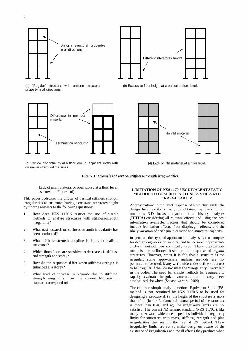
2
Lack of infill material or open storey at a floor level, as shown in Figure 1(d).
This paper addresses the effects of vertical stiffness-strength irregularities on structures having a constant interstorey height by finding answers to the following questions:
1. How does NZS 1170.5 restrict the use of simple methods to analyse structures with stiffness-strength irregularity?
2. What past research on stiffness-strength irregularity has been conducted?
3. What stiffness-strength coupling is likely in realistic structures?
4. Which floor/floors are sensitive to decrease of stiffness and strength at a storey?
5. How do the responses differ when stiffness-strength is enhanced at a storey?
6. What level of increase in response due to stiffness-strength irregularity does the current NZ seismic standard correspond to?
LIMITATION OF NZS 1170.5 EQUIVALENT STATIC METHOD TO CONSIDER STIFFNESS-STRENGTH
IRREGULARITY
Approximations to the exact response of a structure under the design level excitation may be obtained by carrying out numerous 3-D inelastic dynamic time history analyses (IDTHA) considering all relevant effects and using the best information available. Factors that should be considered include foundation effects, floor diaphragm effects, and the likely variation of earthquake demand and structural capacity.
In general, this type of approximate analysis is too complex for design engineers, so simpler, and hence more approximate analysis methods are commonly used. These approximate methods are calibrated based on the response of regular structures. However, when it is felt that a structure is too irregular, some approximate analysis methods are not permitted to be used. Many worldwide codes define structures to be irregular if they do not meet the “irregularity limits” laid in the codes. The need for simple methods for engineers to rapidly evaluate irregular structures has already been emphasized elsewhere (Sadashiva et al. 2009).
The common simple analysis method, Equivalent Static (ES) method is not permitted by NZS 1170.5 to be used for designing a structure if: (a) the height of the structure is more than 10m; (b) the fundamental natural period of the structure is more than 0.4s; and (c) the irregularity limits are not satisfied. The current NZ seismic standard (NZS 1170.5), like many other worldwide codes, specifies individual irregularity limits for structures with mass, stiffness, strength and plan irregularities that restrict the use of ES method. These irregularity limits are set to make designers aware of the existence of irregularities and the ill effects they produce when
Uniform structural properties in all directions
Different interstorey height
Difference in member material
Termination of column
No infill material
(a) “Regular” structure with uniform structural property in all directions.
(b) Excessive floor height at a particular floor level.
(c) Vertical discontinuity at a floor level or adjacent levels with dissimilar structural materials.
(d) Lack of infill material at a floor level.
Figure 1: Examples of vertical stiffness-strength irregularities.

3
a structure has irregularities (SEAOC blue book, 1999). Hence, these individual limits are based on engineering judgement and lack theoretical justification.
Stiffness-strength irregularity, the effects of which are investigated in this study, is said to exist by NZS 1170.5 (Cl. 4.5.1), when:
The lateral stiffness of a storey is less than 70% of the stiffness of any adjacent storey, or less than 80% of the average stiffness of the three storeys above or below in the structure.
The storey shear strength at a floor level is less than 90% that in the storey above.
Although separate irregularity limits are defined for stiffness and strength irregularity, in many practical scenarios, stiffness and strength vary together. For example, when cross-sectional property is changed at a floor level, stiffness and strength at that storey are modified together. Hence, in this paper, stiffness and strength irregularities are combined together and their coupled effects on seismic demands are evaluated.
PREVIOUS RESEARCH ON VERTICAL STIFFNESS-STRENGTH IRREGULARITY
Very few researchers have attempted to investigate the effects of vertical structural irregularities on the seismic response of the structures. Those that have studied have not provided rational justification on the appropriateness of the irregularity limits specified in the NZS 1170.5 and other international codes with the same or similar criteria. An overview of earlier approaches and findings on stiffness-strength effects is summarised below. The stiffness-strength limits for regular buildings, as specified by the Uniform Building Code (UBC) were evaluated by Valmundsson and Nau (1997) by comparing the responses obtained due to time-history analysis using 4 unscaled earthquake records, and the ES method of UBC. Regular structures, represented by plane frames of 5, 10, and 20 storeys, with beams modelled to be stronger than the columns, were defined to have a constant floor mass at each floor level, and a uniform stiffness distribution required to achieve a series of 6 target fundamental periods for each structure height was calculated. First storey stiffness and/or strength of the regular structures were reduced by different amounts to form the irregular structures. A reduction in stiffness alone by 30% was shown to increase the drift by 30% and a decrease in maximum ductility demand by about 20%. Also, this effect on drift was found to decrease with the design ductility. It was found that the ductility demand increased for cases of only first storey strength reduction, and this increase was seen to increase with the structure height and decreased with the design ductility, especially for taller structures. Combined stiffness and strength irregularity cases were created by reducing first storey stiffness and strength proportionally. The ductility demand was found to increase significantly with the height of the building, and this increase was found to be less in case of higher design ductility’s. This study concluded that for a structure to be recognised as being “regular”, the first storey should be stronger than the storey above it.
Al-Ali and Krawinkler (1998) studied the effects of vertical irregularities on height-wise variations of seismic demands by conducting elastic and inelastic dynamic analyses (using 15 records) on 2-D single-bay 10-storey generic structures, assuming the columns to be weaker than the beams. Responses of structures with stiffness or/and strength irregularity were compared with the response of a reference structure that had a uniform distribution of mass over the height and an associated stiffness distribution that resulted in a straight-line first mode shape with storey stiffness’s tuned to
produce a first mode period of 3s when designed according to the modal superposition technique. Stiffness was reduced at the first level or at the mid-height by 0.1, 0.25, and 0.5 times the stiffness at the corresponding floor of the base structure. And, storey stiffness’s of the lower half of the structure was increased by amounts of 2, 4, and 10 times the stiffness at the respective floors of the base case. The stiffness distributions for all the cases were then tuned till the irregular structures had a fundamental period of 3s. Since stiffness irregularities change the distribution of elastic storey shear demands, storey strengths for each of the cases with stiffness irregularities were tuned to their own elastic storey shear distribution obtained from SRSS analyses using the National Earthquake Hazard Reduction Program (NEHRP) spectrum reduced by a strength reduction factor (3 and 6). Storey drift demands were found to increase in the “soft” storey and decrease in most of the other storeys, and the roof drift demands were seen to be less sensitive to the presence of stiffness irregularity. Strength irregularities were introduced by increasing the strength of a specific storey (or storeys) by 2 times the strength of the same storey in the reference base structure, rather than decreasing the storey strength. The stiffness and mass distributions were kept the same as for the base case. It was found that apart from the weak storey (or storeys) at upper half of structure; the roof drift demand did not change by large amounts due to the presence of vertical strength irregularity. Combined stiffness and strength irregularity was limited to cases with equal stiffness and strength modifications by two times the base case stiffness-strength distributions, and was applied at the first level, or the mid-height, or in the lower half of structures. The stiffness-strength distributions at the other floors were kept the same as for their individual irregularity cases. Cases with combined irregularities were shown to generally yield the same trend in responses as the cases with only strength irregularities, but with a larger magnitude.
Chintanapakdee and Chopra (2004) compared the seismic demands for vertically irregular and regular frames of 12 storey height, determined by non-linear response history analysis using a set of 15 earthquake records. For this study, a base case structure, modelled as a beam hinge model, was designed so that the stiffness distribution over the structure height produced equal drifts in all the storeys under the International Building Code (IBC) lateral forces. The target fundamental period was fixed at 2.4s. Numerous irregular frames were obtained by modifying the stiffness or/and strength of the base case by modification factors of 2 and 5. Irregularities were introduced at the first, or the mid-height, or the topmost level, or the lower half of the structure. Stiffness irregular cases were obtained by modifying the stiffness of the chosen irregular floor/floors and tuning the stiffness distribution till the target fundamental period of 2.4s was achieved. All storey strengths were uniformly scaled so that the irregular frames had the same yield base shear as the base case. Cases with only strength irregularity were created by modifying the storey strength of the chosen floor/floors and then uniformly tuning all storey strengths till the irregular frames achieved the same yield base shear as the base case. Combined cases of stiffness-strength irregularity were created by making equal modifications to both the stiffness and strength distributions as described for their individual cases. Like previous researchers, the effects of combined stiffness-strength irregularities were seen to be more influential than any other type of vertical irregularity. Soft and/or weak storey were found to increase the drift demands in the modified and neighbouring storeys, and decreased the drift demands at other storeys. Stiff and/or strong storey decreased the drift demands in the modified and neighbouring storeys and increased the drift demands in other storeys. Effects of an irregular storey on the drift demands in other storeys were strongly dependent on the storey location. These trends described differ from the results obtained from Al-Ali and Krawinkler (1998), where the

4
drift demand was affected only in the soft and/or weak storey having irregularity. It is argued that this is due to their column-hinge model restricting the redistribution of seismic demands to the adjacent storeys. A soft and/or a weak lower half of the frame was shown to slightly increase the drift demands for those storeys, but significantly decreased the drift demands in the storeys at upper half of the frame. In contrast, a stiff and/or strong lower half reduced the drifts for those storeys but significantly increased the drift demands in the upper half of the frame.
A methodology involving incremental dynamic analyses was presented by Michalis et al. (2006) to evaluate the effects of individual stiffness, strength irregularities and also their combined effects. The base structure chosen in this case was a realistic nine storey steel frame, with a higher basement than other floors, and having a fundamental period of 2.25s, and designed for a Los Angeles site. Stiffness and/or strength irregularities were considered by altering the base cases’ stiffness and strength by a factor of 2 and applied at various locations over the height of the structure. The methodology for this study involved performing a series of non-linear dynamic analyses for each of the 20 records selected, by scaling the earthquake records such that the 5% damped first-mode spectral accelerations, Sa (T1, 5%), achieved certain target value. At each scaling level, the maximum interstorey drift ratio, max was obtained. In order to compare the performance of the modified versus the base case, a continuum of limit states was defined, each at a given value of max , spanning all the structural response range from elasticity to global dynamic instability. The distribution of peak interstorey demands over the height of irregular structures, normalised by that due to the base case was found for each irregularity case. At lower intensity levels (0.25-0.5g) and stiffness irregularity at the lower storey, a change of about 30-50% in the drift demand at the modified level was reported. At higher intensity levels, the changes were uniformly distributed, with the maximum change occurring away from the storey where irregularity was introduced. At close to the collapse limit state, about 50% reduction in demands for all the stiffness irregularity cases, irrespective of the position of irregularity or amount of irregularity was observed. Single storey strength reduction along with a soft storey in the basement isolates the yielding in higher levels, and thus has resulted in improved performance, and protecting the building. However, increased strength at lower storeys was shown to produce the opposite effect. For Sa = 0.25g, introducing a weaker/stronger storey at any level of the structure correspondingly increased/decreased the drift demands in the vicinity of modified storey, but had the inverse effect for other floors. Irrespective of the storey modified, a significant change in the drift demand of about 50% was observed at upper floors from all the cases. As the Sa increased, these effects decreased for modifications in the extreme floor levels, but for modifications in the mid-height, it resulted in an uniform change in drift demand along the height of the structure. Stronger/weaker storeys resulted in reduced/increased drift demands at all storeys for these cases. As Sa was increased further, irrespective of amount (+/- strength) and position of modification, a uniform reduction of 50% in drift demands in all storeys was observed. For lower intensity levels (Sa = 0.25-0.75g), the change in drift demand distribution due to combined irregularity, was seen to be qualitatively obtained by adding both the stiffness and strength irregularity results. At 0.25-0.5g levels, upgrading has shown positive effect in the neighbourhood of modification, and inverse effect elsewhere. At higher intensities, upon upgrading/degrading, strong positive/negative effect was observed everywhere, with the maximum being at the storey with the irregularity. At collapse limit state, these effects amplified, with degraded cases reaching global instability and upgraded cases resulting in a uniform 50%-60% decrease in
demands. The influence of multi-storey modifications was quantitatively shown as added effects of corresponding single-storey influences.
As seen from the above review, although most of the methods and findings were consistent between researchers, the works do not clearly justify the irregularity limits in the present codes. As pointed out by the authors in the study on vertical mass irregularity effects (Sadashiva et al. 2009), regular and irregular structures need to be designed for the same engineering demand parameter rather than targeting to achieve a target period. Also, a rigorous study of structures of different heights with realistic correlations between stiffness and strength, which are designed according to the NZ code are required.
METHODOLOGY FOR EVALUATING VERTICAL COUPLED STIFFNESS-STRENGTH IRREGULARITY
EFFECTS
A simple and effective method to provide rational justification for vertical irregularity limits was proposed and applied to structures having vertical mass irregularities (Sadashiva et al. 2009). This simple method is utilised in the present study to evaluate the effects of vertical coupled stiffness-strength irregularities as follows:
1. The peak interstorey drift ratio over all the storeys was chosen as the engineering demand parameter (EDP) to compare the responses of regular and irregular structures with vertical coupled stiffness-strength irregularities.
2. A set of interstorey drift capacities, ranging between 0.5% and 3% were chosen, and for each target interstorey drift capacity, and amount of irregularity: a. Each regular structure was designed to the target
interstorey drift capacity using the NZS 1170.5 ES method.
b. A set of coupled stiffness-strength irregularities were introduced at various locations over the height of the regular structure, and the structures were redesigned using NZS 1170.5 ES method to the same target interstorey drift capacity.
c. The designed regular and irregular structures were then subjected to a suite of scaled earthquake records, and peak interstorey drifts due to the suite of records were obtained.
d. Responses of regular and irregular structures were compared by finding the difference between the median peak interstorey drift responses of the two structures.
3. The performance distributions for the chosen magnitude of irregularity and target interstorey drift ratio were then used to characterise the effect of both of these variables.
DEFINITION OF REGULAR STRUCTURES
Simple models of shear-type building structures of 3, 5, 9 and 15 storeys, having a uniform mass at every floor, and with equal storey height of 4m were adopted to carry out this comprehensive parametric study.
Each regular structure was assumed to be located in Wellington, and was designed according to the NZ 1170.5 ES method considering a set of structural ductility factors of 1, 2, 3, 4, and 6. A complete description on the design approach adopted in this study is explained in Sadashiva et al. (2009). Two classes of regular structures were defined to have:
(a) Decreasing stiffness distribution over the height, with iterations carried out till all floors simultaneously achieved the design (target) interstorey drift ratio (DISDR). Henceforth, this design model is referred as CISDR for constant interstorey drift ratio; and

5
(b) Uniform stiffness distribution up the height, with iterations conducted until the first floor (critical) achieved the target interstorey drift ratio.
In order to have an “apples-to-apples” comparison between regular and irregular structures, each regular design model was provided with storey strengths such that a constant strength to stiffness ratio was maintained at all floor levels. Since a constant strength to stiffness ratio was obtained for CISDR design models at the end of iteration, the shear strength provided at each level was the minimum required to resist the equivalent static design forces. For the design model with constant stiffness distribution, the minimum shear strength required to resist the design force at the first level was provided at all floor levels, thus producing a constant strength to stiffness ratio at all levels. Henceforth, this design model will be referred as CS-CSTG for constant stiffness and strength. Although these two configurations may not necessasarily reflect the actual practical buildings, but these two classes of buildings were assumed to define the bounds within which the realistic structures are assumed to have their configuration. These two models with their configurations are shown in Figure 2.
Unrealistic structures were avoided in this study by eliminating structures having storey strength to stiffness ratios outside the range of 0.3% - 3%. This limit was set based on the likely storey strength to stiffness ratios for realistic structures, determined based on simple and approximate empirical relations (Priestley et al., 2007) giving yield drift ratios for different types of lateral force resisting systems. Also, structures having the horizontal design action coefficient, Cd governed by Equation 2 (Cl. 5.2.1.1, NZS 1170.5) were ignored from this work. That is, for an example of a structure in Wellington, Figure 3 shows coefficient Cd (calculated according to Equation 1) plotted against fundamental period for ductility factors of 1, 2, 4 and 6. The solid line shows the minimum value of this coefficient, Cd,min calculated according to Equation 2.
µkSTC
TC pd
)()( 1
1 = (1)
⎩⎨⎧ +
=u
ud R
RZC
03.0)02.020/(
maxmin, (2)
}{ min,1),(max ddd CTCC = (3)
According to Figure 3, when long period structures are designed to have a design ductility factor, the base shear, calculated based on Equation 3, is governed by the lower limit (Equation 2), making the structures to have an effective ductility factor lower than the design ductility factor. For example, in Figure 3, structures designed to have ductility factor of 2, for periods more than 3.4s, the coefficient Cd is governed by Equation 2, making the structures to have ductility factors between 1 and 2. Hence, structures having the horizontal design action coefficient governed by the lower limit were eliminated from this study.
CORRELATIONS BETWEEN STOREY STIFFNESS AND STRENGTH DUE TO RELATIVE DIFFERENCES
IN MEMBER PROPERTIES
In most practical scenarios, a change in stiffness is accompanied by a change in strength. Therefore, studying stiffness irregularity alone, or strength irregularity alone, while being interesting, does not represent the behaviour of actual structures. The effects of coupled stiffness-strength irregularities, caused due to relative differences in member properties between adjacent storeys are investigated. In this paper, the interstorey height for all irregular structures is kept constant, and equals the interstorey height of regular structures.
0
0.1
0.2
0.3
0.4
0.5
0.6
0.7
0.8
0 1 2 3 4 5
Period, T (s)
Hor
izon
tal D
esig
n A
ctio
n C
oeffi
cien
t, Cd(
T)
µ = 1 µ = 2
µ = 4 µ = 6
Figure 3: Variation of horizontal design action coefficient with fundamental period for Wellington.
⎩⎨⎧ +
=u
ud R
RZC
03.0)02.020/(
maxmin,
µkSTC
TC pd
)()( 1
1 =
Figure 2: Structural configurations defining “regular” structures.
(a) Design forces
F3
F2
F1
V3
V2
V1
V3 = V1
V2 = V1
V1
Design Interstorey Drift Ratio (DISDR)
DISDR M
M
M
K3
K2
K1
(b) CISDR design
(c) Stiffness dist. for CISDR design
(d) Strength dist. for CISDR design
(e) Drift dist. for CISDR design
M
M
M
K3
K2
K1
(f) CS-CSTG design
(g) Stiffness dist. for CS-CSTG design
(h) Strength dist. for CS-CSTG design
(i) Drift dist. for CS-CSTG design

6
Depending on the type of lateral-force-resisting (LFR) system, the storey strength can vary proportionally or by differing amounts when the storey stiffness is modified. Relations between storey stiffness and strength were obtained for few common LFR systems used to resist seismic forces as shown in Table 2. Here, the modified lateral stiffness at a chosen floor level for irregularity, irrespective of the LFR system, Km, is given as the product of the stiffness modification factor, k and the initial lateral stiffness at the chosen level, Ko. The modified storey strength provided at the chosen floor level, Vm, for braced frames and shear wall type of LRF systems, is given as the product of stiffness modification factor and the initial storey strength provided for the floor level, Vo. However, in case of moment frames, an additional strength modification factor, , representing the modification in strength when the member section depth in the regular structure, do, is modified to dm, is applied along with the stiffness modification factor. The value of is assumed to vary between 1 and 1.5 for stiffness reduction cases, and for stiffness enhancement cases, its magnitude is taken as between 0.67 and 1.
Thus, two groups, based on these relations between storey stiffness and strength were formed to define the types of irregular structures used to evaluate their coupled effects. In Table 1, Group A represents braced frame and shear wall types of LFR systems having strength varying proportionally with stiffness, and Group B represents stiffness-strength coupling relation for moment frames. In order to investigate the sensitivity of magnitude of irregularities on seismic demands, a range of stiffness-strength modification factors, as tabulated in Table 1, covering cases of storey stiffness and strength enhancement or reduction, were used. Here, for each modification in storey stiffness by k in Group B, all the three selected values for each case were applied, thus resulting in a total of 18 combinations for this group.
Case: Group A Group B
Stiffness enhancement
k
Stiffness enhancement
1.2, 1.5, 2
1
Stiffness enhancement
1.2, 1.5, 2
0.7, 0.8, 0.9
Stiffness reduction
k
Stiffness enhancement for
0.5, 0.6, 0.7, 0.8, 0.9
1
Stiffness enhancement
0.5, 0.7, 0.9
1.1, 1.3, 1.5
Table 1: Cases defining structures with coupled vertical stiffness-strength irregularities.

7
Lateral-force-resisting (LFR) system Modified storey stiffness, Km Modified storey strength, Vm
(a) Braced Frame
δx
δa
Ha
F
h
L
θ
22 hL
EAK a
+=
22 hL
LAV yaa
+=
σ
⎟⎟⎟
⎠
⎞
⎜⎜⎜
⎝
⎛ +
⎟⎟⎟
⎠
⎞
⎜⎜⎜
⎝
⎛
+=
EAhL
hL
EAKK
ao
am
o
m22
22*
oao
amm K
AA
K *⎟⎟⎠
⎞⎜⎜⎝
⎛=
okm KK *α=
hL
hEAhL
hL
LAhK
V y
a
yaa εσ=
⎟⎟⎟
⎠
⎞
⎜⎜⎜
⎝
⎛ +
⎟⎟⎟
⎠
⎞
⎜⎜⎜
⎝
⎛
+= 1**
22
22
⎟⎟⎠
⎞⎜⎜⎝
⎛⎟⎟⎠
⎞⎜⎜⎝
⎛=
⎟⎠⎞⎜⎝
⎛
⎟⎠⎞⎜⎝
⎛
Lh
hL
hKV
hKV
y
y
oo
mm
εε
*
oo
mm V
KK
V *⎟⎟⎠
⎞⎜⎜⎝
⎛=
okm VV *α=
(b) Shear Wall
h
δs F
L
hAGK s=
3ysA
Vσ
=
⎟⎟⎠
⎞⎜⎜⎝
⎛⎟⎟⎠⎞
⎜⎜⎝⎛=
so
sm
o
mAGh
hAG
KK
*
oso
smm K
AA
K *⎟⎟⎠
⎞⎜⎜⎝
⎛=
okm KK *α=
31**
3 GhAGhA
hKV y
s
ys σσ=⎟⎟⎠
⎞⎜⎜⎝
⎛⎟⎟⎠
⎞⎜⎜⎝
⎛=
⎟⎟⎠
⎞⎜⎜⎝
⎛⎟⎟⎠
⎞⎜⎜⎝
⎛=
⎟⎠⎞⎜⎝
⎛
⎟⎠⎞⎜⎝
⎛
y
y
oo
mm
GG
hKV
hKV
σσ 3*
3
oo
mm V
KK
V *⎟⎟⎠
⎞⎜⎜⎝
⎛=
okm VV *α=
(c) Moment Frame (strong column weak beam mechanism)
Mp
h
L
∆
F
26
hLIE
K = h
MV p=
⎟⎟⎠
⎞⎜⎜⎝
⎛⎟⎟⎠
⎞⎜⎜⎝
⎛=
o
m
o
mIE
hLhLIE
KK
6*6 2
2
oo
mm K
II
K *⎟⎟⎠
⎞⎜⎜⎝
⎛=
okm KK *α=
hIEhL
hM
hKV p 1*
6*
2
⎟⎟⎠
⎞⎜⎜⎝
⎛⎟⎟⎠
⎞⎜⎜⎝
⎛=
6
*2
6* L
dL
IEM yp
⎟⎟⎠
⎞⎜⎜⎝
⎛=⎟⎟⎠
⎞⎜⎜⎝
⎛=
ε
⎟⎟⎠
⎞⎜⎜⎝
⎛=
⎟⎠⎞⎜⎝
⎛
⎟⎠⎞⎜⎝
⎛
m
o
oo
mm
dd
hKV
hKV
om
o
o
mm V
dd
KK
V ** ⎟⎟⎠
⎞⎜⎜⎝
⎛⎟⎟⎠
⎞⎜⎜⎝
⎛=
okm VV **γα=
(d) Moment Frame (strong beam weak column mechanism)
F
h
Mp
L
312
hIE
K = hM
V p2=
⎟⎟⎠
⎞⎜⎜⎝
⎛⎟⎟⎠
⎞⎜⎜⎝
⎛=
o
m
o
mIE
hh
IEKK
12*12 3
3
oo
mm K
II
K *⎟⎟⎠
⎞⎜⎜⎝
⎛=
okm KK *α=
6*
21*12
*2 3 h
dhIEh
hM
hKV yp
⎟⎟⎠
⎞⎜⎜⎝
⎛=⎟
⎟⎠
⎞⎜⎜⎝
⎛⎟⎟⎠
⎞⎜⎜⎝
⎛=
ε
⎟⎟⎠
⎞⎜⎜⎝
⎛=
⎟⎠⎞⎜⎝
⎛
⎟⎠⎞⎜⎝
⎛
m
o
oo
mm
dd
hKV
hKV
om
o
o
mm V
dd
KK
V ** ⎟⎟⎠
⎞⎜⎜⎝
⎛⎟⎟⎠
⎞⎜⎜⎝
⎛=
okm VV **γα=
Table 2: Correlations between storey stiffness-strength due to modified member properties.

8
APPLYING COUPLED STIFFNESS AND STRENGTH IRREGULARITIES
The effect of coupled stiffness-strength over the height of the structures was conducted by applying the irregularities at the first level, or at the mid-height, or at the topmost floor level of regular structures. This was done by introducing the stiffness modification factor at the chosen regular floor level, and then redesigning the modified structure until the target interstorey drift ratio is achieved at the critical floor level. For example, as shown in Figure 4, consider a regular 3 storey CS-CSTG structure designed for a structural ductility factor of 4, and having a uniform stiffness distribution resulting in a target interstorey drift ratio (DISDR) of 1% at the first floor level. If it is intended to have a soft storey at the third floor, the storey stiffness of the regular structure at that level is reduced by means of stiffness modification factor, k, by an amount of say, 0.5. Upon making this change in storey stiffness, the critical floor would no longer have the chosen DISDR. In order to compare the responses of regular and irregular structures, all storey stiffness are then uniformly scaled by a scaling factor, , and the irregular structure is redesigned till the chosen DISDR is achieved at the critical floor. Since all storey stiffness’s are uniformly scaled, at the end of iteration, the irregular structure would still maintain the applied k at the chosen floor level, which is third floor in this example. However, the relative storey stiffness’s at other floors remain unchanged and equal the corresponding storey stiffness’s of regular structure. The storey strength distribution is similarly modified at the chosen floor level according to Equation 4, and uniformly scaled with the factor.
okm VV γα= (4)
STRUCTURAL MODELLING AND ANALYSIS
Earlier studies (e.g., MacRae et al. 2004, Tagawa et al. 2006) on structural modelling have shown that the frames modelled as a combination of vertical shear beam and a vertical flexural column (labelled as SFB in Figure 5) can represent the behaviour of real structures well. If the flexural beam is not considered, unrealistically high drift concentrations may occur. The flexural beam represents all continuous columns throughout the whole structure. The flexural beam stiffness ratio, cc, in actual structure tends to be greater than 0.5, so this value at all levels was used in all analyses. EI was computed for the flexural beam from the equation in Figure 5. Sadashiva et al. (2009) have also shown that the regular structures modelled without the flexural beam have increased
median interstorey drift demands. This increase in demand was observed to increase with the height of the structure, and about 50% increase in median interstorey drift demand was observed for 9 storey structures.
Figure 5: Combined vertical Shear and Flexural Beam (SFB model).
A set of 20 SAC (SEAOC-ATC-CUREE) earthquake ground motion records for Los Angeles, with probabilities of exceedance of 10% in 50 years, were used for the ground motion suite. Response spectra were developed for each of the selected records and the accelerations within each record were scaled so that its single-degree-of-freedom elastic displacement response spectrum matched the design interstorey drift for NZS 1170.5 in the city chosen. Here, both the structural ductility factor and the structural performance factor were unity.
Rayleigh damping has commonly been adopted to represent damping effects within multi-degree-of-freedom structures for several decades. A recent study by Sadashiva et al. (2009) on the effects of different types of Rayleigh damping models show that the differences in drift responses due to three types of Rayleigh damping models available in RUAUMOKO (Carr 2004) time-history program were minimal. However, the tangent stiffness proportional Rayleigh damping model that uses the absolute form of equation of motion was considered to be more appropriate than other types of Rayleigh damping, to be used in IDTHA. Such a damping model that considers the non-linearity effects of structures, also assures that the damping forces go to zero at the end of excitation, and hence it has been used for all IDTHA conducted in this work. In order to avoid super-critical damping or negative damping, the first mode and the mode corresponding to number of storeys in the structure (Carr 2004) were nominated as the two modes with 5% of critical damping. The RUAUMOKO computer program was used to carry out all the inelastic dynamic time-history analysis considering a post elastic stiffness (bilinear) factor of 1%.
Interpretation of Inelastic Dynamic Time-History Analysis Results
The peak interstorey drift ratio (ISDR) at every floor level, and within the structure, when subjected to each of the 20 earthquake records, was obtained. It was assumed that the distribution of ISDR is lognormal (Cornell et al. 2002), so the median and dispersion were found to measure the likely and the spread in the results respectively, as per Equations 5 and 6.
( )⎟⎟
⎠
⎞⎜⎜
⎝
⎛∑
==
n
iix
nex 1
ln1
ˆ (5)
( )∑=
−−
=n
iix xx
n1
2ln ˆlnln
)1(1σ (6)
where xi = peak interstorey drift ratio due to ith record; and
n = total number of earthquake records considered.
∆n
∆2
∆1
∆n-1
Rigid Link
Pin
Shear-Beam Flexural-Beam
∆n
∆2
∆1
∆n-1
Rigid Link
Pin
Shear-Beam Flexural-Beam
oii
icci
KH
IE3=α
where αcci = continuous column stiffness ratio at level, i;E = elastic modulus;Ii = moment of inertia at the ith level;
Hi = storey height of the ith level; andKoi = lateral initial stiffness of the ith level.
∆n
∆2
∆1
∆n-1
Rigid Link
Pin
Shear-Beam Flexural-Beam
∆n
∆2
∆1
∆n-1
Rigid Link
Pin
Shear-Beam Flexural-Beam
oii
icci
KH
IE3=α
where αcci = continuous column stiffness ratio at level, i;E = elastic modulus;Ii = moment of inertia at the ith level;
Hi = storey height of the ith level; andKoi = lateral initial stiffness of the ith level.
Ko
Ko
Ko
ho
ho
ho
F3
F2
F1
Km = k Ko ho
ho
ho
Ko
Ko
Km = k Ko ho
ho
ho
Ko
Ko
(a) Design forces
(b) Regular CS-CSTG design with DISDR at first floor
(c) Introducing stiffness modification at third floor
(d) Irregular structure with DISDR at critical floor
Figure 4: Stiffness irregularity introduced by changing member property for CS-CSTG design.

9
Comparison between IDTHA and ES method responses: At each of the design (target) interstorey drift ratio, the median of peak interstorey drift ratios at each of the floor level due to the IDTHA method was compared with the corresponding ES method responses. Such a comparison was carried out for both regular as well as irregular structures. For brevity, however, representative results for regular and Group A irregular structures only are presented in the following paragraphs. The response plot labels in the following figures have the format “N-L(Q)”, where N refers to the number of storeys in the structure, L refers to the location (floor level) of the irregularity and Q defines the magnitude of irregularity (stiffness modification factor).
For 9 storey regular CISDR designs, as shown in Figure 6(a), the ES method gives a good estimate of peak interstorey drift ratio. For many floors, for all DISDR values it is seen that the code estimation of storey drifts are conservative, and the differences between the actual and the ES method drift predictions at these floors are shown to increase with the DISDR.
In case of 9 storey regular CS-CSTG design, as shown in Figure 6(b), the first two floors have median drifts greater than the target DISDR of 0.5%. At other target DISDR’s, the ES method estimates the median drifts well at the top and bottom storeys of the structure, but it was conservative at the intermediate levels.
For CISDR designs with a structural ductility factor of 3, the average increase in median ISDR for 9 and 15 storey regular structures as compared to the ES method drift prediction were found as 19% and 44% respectively. For CS-CSTG designs, ES method did not always under predict the responses. That is, median ISDR of 17% and 5% on average was observed to be less than the ES method drift predictions for 9 and 15 storey structures respectively. For these two storey heights, the median ISDR on average was found to be 15% and 29% more than the corresponding ES method prediction.
0 0.25 0.5 0.75 11
2
3
4
5
6
7
8
9
Interstorey Drift Ratio (%)
Sto
rey
ES MethodITHA Method
0.5 1 1.5 21
2
3
4
5
6
7
8
9
Interstorey Drift Ratio (%)
Sto
rey
ES MethodITHA Method
1 1.5 2 2.5 31
2
3
4
5
6
7
8
9
Interstorey Drift Ratio (%)
Sto
rey
ES MethodITHA Method
0 0.25 0.5 0.75 11
2
3
4
5
6
7
8
9
Interstorey Drift Ratio (%)
Sto
rey
ES MethodITHA Method
0 0.5 1 1.5 21
2
3
4
5
6
7
8
9
Interstorey Drift Ratio (%)
Sto
rey
ES MethodITHA Method
0 0.5 1 1.5 2 2.5 31
2
3
4
5
6
7
8
9
Interstorey Drift Ratio (%)
Sto
rey
ES MethodITHA Method
(1) DISDR = 0.5% (2) DISDR = 1.5% (3) DISDR = 2.5%
(b) CS-CSTG design
Figure 6: Comparison between ES method and IDTHA median interstorey drift ratios for regular designs. (No. of storeys: 9, = 3, Z = 0.4)
(1) DISDR = 0.5% (2) DISDR = 1.5% (3) DISDR = 2.5%
(a) CISDR design
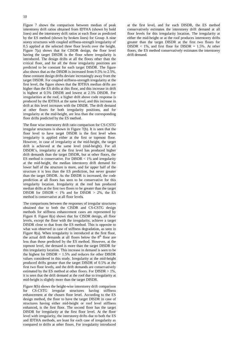
10
Figure 7 shows the comparison between median of peak interstorey drift ratios obtained from IDTHA (shown by bold lines) and the interstorey drift ratios at each floor as predicted by the ES method (shown by broken lines) for Group A nine storey structures with coupled stiffness-strength irregularity of 0.5 applied at the selected three floor levels over the height. Figure 7(a) shows that for CISDR design, the floor level having the target DISDR is the floor where irregularity is introduced. The design drifts at all the floors other than the critical floor, and for all the three irregularity positions are predicted to be constant for each target DISDR. The figure also shows that as the DISDR is increased from 0.5% to 2.5%, these constant design drifts deviate increasingly away from the target DISDR. For coupled stiffness-strength irregularity at the first level, the figure shows that the IDTHA median drifts are higher than the ES drifts at this floor, and this increase in drift is highest at 0.5% DISDR and lowest at 2.5% DISDR. For irregularities at the roof, a higher drift above code response is produced by the IDTHA at the same level, and this increase in drift at this level increases with the DISDR. The drift demand at other floors for both irregularity positions, and for irregularity at the mid-height, are less than the corresponding floor drifts predicted by the ES method.
The floor wise interstorey drift ratio comparison for CS-CSTG irregular structures is shown in Figure 7(b). It is seen that the floor level to have target DISDR is the first level when irregularity is applied either at the first or topmost floor. However, in case of irregularity at the mid-height, the target drift is achieved at the same level (mid-height). For all DISDR’s, irregularity at the first level has produced higher drift demands than the target DISDR, but at other floors, the ES method is conservative. For DISDR < 1% and irregularity at the mid-height, the median interstorey drift demand for lower half of the structure is more, and for upper half of the structure it is less than the ES prediction, but never greater than the target DISDR. As the DISDR is increased, the code prediction at all floors has seen to be conservative for this irregularity location. Irregularity at the roof has produced median drifts at the first two floors to be greater than the target DISDR for DISDR < 1% and for DISDR > 2%, the ES method is conservative at all floor levels.
The comparisons between the responses of irregular structures obtained due to both the CISDR and CS-CSTG design methods for stiffness enhancement cases are represented by Figure 8. Figure 8(a) shows that for CISDR design, all floor levels, except the floor with the irregularity, achieve a target DISDR close to that from the ES method. This is opposite to what was observed in case of stiffness degradation, as seen in Figure 8(a). When irregularity is introduced at the first floor, the actual drift demands at all floors below the 8th floor are less than those predicted by the ES method. However, at the topmost level, the demand is more than the target DISDR for this irregularity location. This increase in demand is seen to be the highest for DISDR = 1.5% and reduces for other DISDR values considered in this study. Irregularity at the mid-height produced drifts greater than the target DISDR of 0.5% at the first two floor levels, and the drift demands are conservatively estimated by the ES method at other floors. For DISDR > 1%, it is seen that the drift demand at the roof due to irregularity at mid-height is slightly more than the target DISDR.
Figure 8(b) shows the height-wise interstorey drift comparison for CS-CSTG irregular structures having stiffness enhancement at the chosen floor level. According to the ES design method, the floor to have the target DISDR in case of structures having either mid-height or roof level stiffness enhanced, is the first floor. The second floor has the target DISDR for irregularity at the first floor level. At the floor level with irregularity, the interstorey drifts due to both the ES and IDTHA methods, are least for each case of irregularity as compared to drifts at other floors. For irregularity introduced
at the first level, and for each DISDR, the ES method conservatively estimates the interstorey drift demand at all floor levels for this irregularity location. The irregularity at either the mid-height or at the roof produces interstorey drifts greater than the target DISDR at the first two floors for DISDR < 1%, and first floor for DISDR = 1.5%. At other floors, the ES method conservatively estimates the interstorey drift demand.

11
0 0.25 0.5 0.75 1 1.25 1.51
2
3
4
5
6
7
8
9
Interstorey Drift Ratio (%)
Sto
rey
9-1(0.5)9-5(0.5)9-9(0.5)
0 0.5 1 1.5 2 2.5 31
2
3
4
5
6
7
8
9
Interstorey Drift Ratio (%)
Sto
rey
9-1(0.5)9-5(0.5)9-9(0.5)
0.5 1 1.5 2 2.5 3 3.5 4 4.5 51
2
3
4
5
6
7
8
9
Interstorey Drift Ratio (%)
Sto
rey
9-1(0.5)9-5(0.5)9-9(0.5)
0 0.25 0.5 0.75 11
2
3
4
5
6
7
8
9
Interstorey Drift Ratio (%)
Sto
rey
9-1(0.5)9-5(0.5)9-9(0.5)
0 0.5 1 1.5 2 2.5
1
2
3
4
5
6
7
8
9
Interstorey Drift Ratio (%)
Sto
rey
9-1(0.5)9-5(0.5)9-9(0.5)
0 0.5 1 1.5 2 2.5 31
2
3
4
5
6
7
8
9
Interstorey Drift Ratio (%)
Sto
rey
9-1(0.5)9-5(0.5)9-9(0.5)
0 0.25 0.5 0.75 11
2
3
4
5
6
7
8
9
Interstorey Drift Ratio (%)
Sto
rey
9-1(2)9-5(2)9-9(2)
0 0.5 1 1.5 2
1
2
3
4
5
6
7
8
9
Interstorey Drift Ratio (%)
Sto
rey
9-1(2)9-5(2)9-9(2)
0.5 1 1.5 2 2.5 31
2
3
4
5
6
7
8
9
Interstorey Drift Ratio (%)
Sto
rey
9-1(2)9-5(2)9-9(2)
0 0.25 0.5 0.75 11
2
3
4
5
6
7
8
9
Interstorey Drift Ratio (%)
Sto
rey
9-1(2)9-5(2)9-9(2)
0 0.5 1 1.5 21
2
3
4
5
6
7
8
9
Interstorey Drift Ratio (%)
Sto
rey
9-1(2)9-5(2)9-9(2)
0 0.5 1 1.5 2 2.5 31
2
3
4
5
6
7
8
9
Interstorey Drift Ratio (%)
Sto
rey
9-1(2)9-5(2)9-9(2)
(1) DISDR = 0.5% (2) DISDR = 1.5% (3) DISDR = 2.5%
(a) CISDR design
(1) DISDR = 0.5% (2) DISDR = 1.5% (3) DISDR = 2.5%
(b) CS-CSTG design
Figure 7: Comparison between ES method and IDTHA median interstorey drift ratios for Group A irregular structures with stiffness-strength reduction. (No. of storeys: 9, = 3, Z = 0.4, k = 0.5)
(1) DISDR = 0.5% (2) DISDR = 1.5% (3) DISDR = 2.5%
(a) CISDR design
(1) DISDR = 0.5% (2) DISDR = 1.5% (3) DISDR = 2.5%
(b) CS-CSTG design
Figure 8: Comparison between ES method and IDTHA median interstorey drift ratios for Group A irregular structures with stiffness-strength enhancement. (No. of storeys: 9, = 3, Z = 0.4, k = 2)
12
Comparison between regular and irregular structures – effect of magnitude and location of coupled vertical stiffness-strength irregularity: The effects of coupled vertical stiffness-strength irregularities on the responses of 3, 5, 9, and 15 storey structures was carried out by introducing irregularities at a particular floor level of the regular structure, and redesigning the irregular structure till the critical floor achieved the same target design interstorey drift ratio as the regular structure, when designed according to the ES method of NZS 1170.5. Lateral strength and stiffness at the first level, or the mid-height, or the topmost floor level of regular structures were either increased or decreased by the same amount (Group A) or by unequal amounts (Group B). The actual peak interstorey drift demands were obtained by subjecting both the regular as well as the irregular structures to a suite of 20 scaled earthquake records. The median of peak interstorey drift ratio (ISDR) obtained for each irregular structure has been compared with the corresponding ISDR of regular structure. The change in median ISDR due to the presence of coupled stiffness-strength irregularity has been used to show the effects of irregularity in the following section. However, for brevity, representative results obtained for structures designed for structural ductility factor of 3 have only been shown in Figures 9 through 12. As explained earlier, the structures having unrealistic strength to stiffness ratios and/or having the base shear governed by the lower limit were eliminated from this study. Hence, some of the following response plots have limited results due to these two conditions imposed in the design.
Comparison of responses for Group A structures: For CISDR designs, the median ISDR’s obtained for both the regular and irregular structures with stiffness-strength decreased storeys, are plotted against DISDR in Figure 9. The figure shows that for the least stiffness modification factor, k of 0.5 introduced at the first floor, higher median ISDR than for the regular structure is obtained for taller structures designed for DISDR < 2%. A maximum of 77% and 40% increase in median drift demand over the regular structure is observed for 9 and 15 storey structures respectively, designed for DISDR = 0.5% and having k of 0.5 at the first level. For 3 storey structures, this increase in demand is 16% for DISDR = 1%. When coupled stiffness-strength irregularity of 0.5 is introduced at the mid-height of all structures, the median drift demands are lesser than those for regular structures for all DISDR’s. Taller structures designed for DISDR > 1% produced higher drifts than the regular structure when the stiffness and strength of the topmost floor is reduced by 0.5. The maximum increase in median ISDR due to irregularity at the roof from all DISDR’s is 15%, 56%, and 52% for 3, 9, and 15 storeys respectively. As expected, when the stiffness modification ratio is increased from 0.5 to 0.9 at the three irregular floors, the differences in responses between regular and irregular structures are reduced. Irregularities at the topmost level have tended to produce higher drifts than the other two positions, and the maximum increase in median ISDR over the regular structures from all structure heights, are 42%, 23%, 10% and 1.2% for k = 0.6, 0.7, 0.8, and 0.9 respectively.
Response comparison between the regular and irregular structures for CS-CSTG design is shown in Figure 9(b). Irregular structures created by reducing the first storey stiffness and strength have shown to produce the largest change in median ISDR compared to other two irregular positions over the height of all structure heights considered in this study. For k = 0.5 at the first level, the median ISDR increases with the structure height, as shown in Figure 9(b). The maximum increase in drift demand over the regular
structures is found to be 30%, 48%, and 83% for 3, 9, and 15 storey structures respectively. Similar to the CISDR design, irregularity at the mid-height has shown to produce drifts lesser than the regular structure for all structures, and the structures with topmost floor with reduced stiffness-strength has median ISDR closely matching with the response of the regular structure for most of the DISDR values and for all the structure heights. The influence of stiffness modification factor on the responses reduces as the factor k is increased from 0.5 up to 0.9. The maximum increase in median ISDR due to irregularity at the first level, obtained from all structural heights, is found to be 45%, 29%, 23%, and 10% for k = 0.6, 0.7, 0.8, and 0.9 respectively.
Figure 10(a) shows the median ISDR response plots for the regular and irregular structures having stiffness-strength increased at a chosen floor level. Three storeys irregular structures created using factor k = 1.2 produced smaller drifts than the regular structures. For taller structures, with this k at the mid-height, a maximum increase in median ISDR of 2.6% and 1.6% was found for 9 and 15 storey high structures respectively. Irregularity at the roof produced drifts less than those for the regular structures for all the structural heights and DISDR. Differences in responses between the regular and irregular structures increased with an increase in the factor k, as shown in Figure 10(a). As k was increased from 1.2 to 2, the coupled stiffness-strength irregularity introduced at the first floor for 3 storey structure, and for the 15 storey structure it was the mid-height that generally produced higher median ISDR. In case of nine storey structures, irregularities at both these floor levels tended to giver higher drift demands as shown in the figure. The maximum increase in median ISDR for 3, 9, and 15 storey structures is found to be 15%, 12%, and 4.5% respectively.
The effect of a storey having stiffness-strength increased for CS-CSTG designs is shown in Figure 10(b). Nine and 15 storey structures with the first floor stiffness-strength increased by k = 1.2 performed better than the regular structures. However, in case of a 3 storey structure having the same magnitude of irregularity and located at the same floor, a maximum increase in ISDR of 26% is obtained for DISDR = 0.5%. As k was increased up to 2, the figure shows that irrespective of the structure height, irregularity at the first level helped performance of the irregular structures compared to the regular structures. Similar to the CS-CSTG design with stiffness degradation case, the irregularity at the topmost level has drift demands closely matching with the corresponding drifts of the regular structures for many DISDR’s. But, in case of irregularity at the mid-height, which was generally seen to perform better than the regular structures for CS-CSTG design with stiffness degradation, is however in this case of stiffness enhancement has produced a maximum increase in median ISDR of 25%.
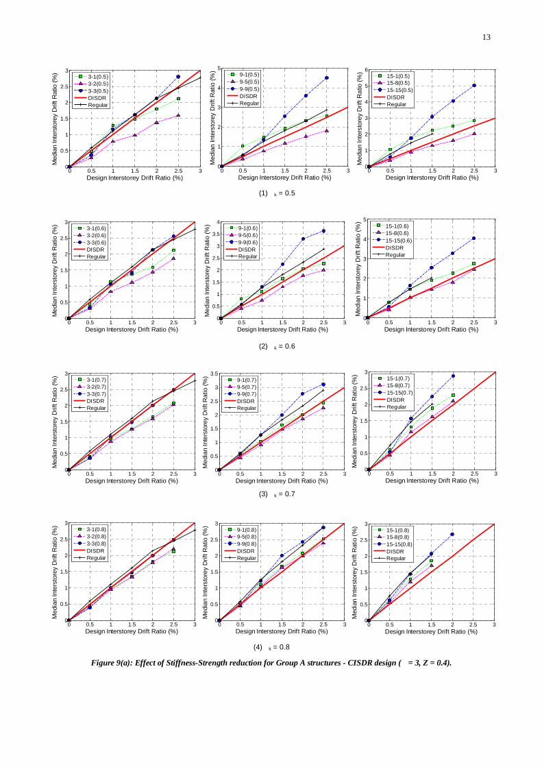
13
0 0.5 1 1.5 2 2.5 30
0.5
1
1.5
2
2.5
3
Design Interstorey Drift Ratio (%)
Med
ian
Inte
rsto
rey
Drif
t Rat
io (%
) 3-1(0.5)3-2(0.5)3-3(0.5)DISDRRegular
0 0.5 1 1.5 2 2.5 3
0
1
2
3
4
5
Design Interstorey Drift Ratio (%)
Med
ian
Inte
rsto
rey
Drif
t Rat
io (%
) 9-1(0.5)9-5(0.5)9-9(0.5)DISDRRegular
0 0.5 1 1.5 2 2.5 3
0
1
2
3
4
5
6
Design Interstorey Drift Ratio (%)
Med
ian
Inte
rsto
rey
Drif
t Rat
io (%
)
15-1(0.5)15-8(0.5)15-15(0.5)DISDRRegular
0 0.5 1 1.5 2 2.5 30
0.5
1
1.5
2
2.5
3
Design Interstorey Drift Ratio (%)
Med
ian
Inte
rsto
rey
Drif
t Rat
io (%
) 3-1(0.6)3-2(0.6)3-3(0.6)DISDRRegular
0 0.5 1 1.5 2 2.5 3
0
0.5
1
1.5
2
2.5
3
3.5
4
Design Interstorey Drift Ratio (%)
Med
ian
Inte
rsto
rey
Drif
t Rat
io (%
) 9-1(0.6)9-5(0.6)9-9(0.6)DISDRRegular
0 0.5 1 1.5 2 2.5 3
0
1
2
3
4
5
Design Interstorey Drift Ratio (%)
Med
ian
Inte
rsto
rey
Drif
t Rat
io (%
)
15-1(0.6)15-8(0.6)15-15(0.6)DISDRRegular
0 0.5 1 1.5 2 2.5 30
0.5
1
1.5
2
2.5
3
Design Interstorey Drift Ratio (%)
Med
ian
Inte
rsto
rey
Drif
t Rat
io (%
) 3-1(0.7)3-2(0.7)3-3(0.7)DISDRRegular
0 0.5 1 1.5 2 2.5 3
0
0.5
1
1.5
2
2.5
3
3.5
Design Interstorey Drift Ratio (%)
Med
ian
Inte
rsto
rey
Drif
t Rat
io (%
) 9-1(0.7)9-5(0.7)9-9(0.7)DISDRRegular
0 0.5 1 1.5 2 2.5 3
0
0.5
1
1.5
2
2.5
3
Design Interstorey Drift Ratio (%)
Med
ian
Inte
rsto
rey
Drif
t Rat
io (%
) 15-1(0.7)15-8(0.7)15-15(0.7)DISDRRegular
0 0.5 1 1.5 2 2.5 30
0.5
1
1.5
2
2.5
3
Design Interstorey Drift Ratio (%)
Med
ian
Inte
rsto
rey
Drif
t Rat
io (%
) 3-1(0.8)3-2(0.8)3-3(0.8)DISDRRegular
0 0.5 1 1.5 2 2.5 3
0
0.5
1
1.5
2
2.5
3
Design Interstorey Drift Ratio (%)
Med
ian
Inte
rsto
rey
Drif
t Rat
io (%
)
9-1(0.8)9-5(0.8)9-9(0.8)DISDRRegular
0 0.5 1 1.5 2 2.5 3
0
0.5
1
1.5
2
2.5
3
Design Interstorey Drift Ratio (%)
Med
ian
Inte
rsto
rey
Drif
t Rat
io (%
)
15-1(0.8)15-8(0.8)15-15(0.8)DISDRRegular
(1) k = 0.5
(2) k = 0.6
(3) k = 0.7
(4) k = 0.8
Figure 9(a): Effect of Stiffness-Strength reduction for Group A structures - CISDR design ( = 3, Z = 0.4).

14
0 0.5 1 1.5 2 2.5 30
0.5
1
1.5
2
2.5
3
Design Interstorey Drift Ratio (%)
Med
ian
Inte
rsto
rey
Drift
Rat
io (%
) 3 -1(0.5)3-2(0.5)3-3(0.5)DISDRRegular
0 0.5 1 1.5 2 2.5 3
0
0.5
1
1.5
2
2.5
3
3.5
Design Interstorey Drift Ratio (%)
Med
ian
Inte
rsto
rey
Drif
t Rat
io (%
)
9-1(0.5)9-5(0.5)9-9(0.5)DISDRRegular
0 0.5 1 1.5 2 2.5 3
0
0.5
1
1.5
2
2.5
3
3.5
Design Interstorey Drift Ratio (%)
Med
ian
Inte
rsto
rey
Drif
t Rat
io (%
) 15-1(0.5)15-8(0.5)15-15(0.5)DISDRRegular
0 0.5 1 1.5 2 2.5 30
0.5
1
1.5
2
2.5
3
Design Interstorey Drift Ratio (%)
Med
ian
Inte
rsto
rey
Drif
t Rat
io (%
) 3-1(0.6)3-2(0.6)3-3(0.6)DISDRRegular
0 0.5 1 1.5 2 2.5 3
0
0.5
1
1.5
2
2.5
3
Design Interstorey Drift Ratio (%)
Med
ian
Inte
rsto
rey
Drif
t Rat
io (%
)
9-1(0.6)9-5(0.6)9-9(0.6)DISDRRegular
0 0.5 1 1.5 2 2.5 3
0
0.5
1
1.5
2
2.5
3
Design Interstorey Drift Ratio (%)
Med
ian
Inte
rsto
rey
Drif
t Rat
io (%
)
15-1(0.6)15-8(0.6)15-15(0.6)DISDRRegular
0 0.5 1 1.5 2 2.5 30
0.5
1
1.5
2
2.5
3
Design Interstorey Drift Ratio (%)
Med
ian
Inte
rsto
rey
Drif
t Rat
io (%
) 3-1(0.7)3-2(0.7)3-3(0.7)DISDRRegular
0 0.5 1 1.5 2 2.5 3
0
0.5
1
1.5
2
2.5
3
Design Interstorey Drift Ratio (%)
Med
ian
Inte
rsto
rey
Drif
t Rat
io (%
)
9-1(0.7)9-5(0.7)9-9(0.7)DISDRRegular
0 0.5 1 1.5 2 2.5 3
0
0.5
1
1.5
2
2.5
3
Design Interstorey Drift Ratio (%)
Med
ian
Inte
rsto
rey
Drif
t Rat
io (%
)
15-1(0.7)15-8(0.7)15-15(0.7)DISDRRegular
0 0.5 1 1.5 2 2.5 30
0.5
1
1.5
2
2.5
3
Design Interstorey Drift Ratio (%)
Med
ian
Inte
rsto
rey
Drif
t Rat
io (%
) 3-1(0.8)3-2(0.8)3-3(0.8)DISDRRegular
0 0.5 1 1.5 2 2.5 3
0
0.5
1
1.5
2
2.5
3
Design Interstorey Drift Ratio (%)
Med
ian
Inte
rsto
rey
Drif
t Rat
io (%
)
9-1(0.8)9-5(0.8)9-9(0.8)DISDRRegular
0 0.5 1 1.5 2 2.5 3
0
0.5
1
1.5
2
2.5
3
Design Interstorey Drift Ratio (%)
Med
ian
Inte
rsto
rey
Drif
t Rat
io (%
)
15-1(0.8)15-8(0.8)15-15(0.8)DISDRRegular
(1) k = 0.5
(2) k = 0.6
(3) k = 0.7
(4) k = 0.8
Figure 9(b): Effect of Stiffness-Strength reduction for Group A structures – CS-CSTG design ( = 3, Z = 0.4).
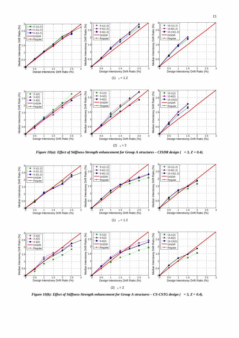
15
0 0.5 1 1.5 2 2.5 30
0.5
1
1.5
2
2.5
3
Design Interstorey Drift Ratio (%)
Med
ian
Inte
rsto
rey
Drift
Rat
io (%
) 3-1(1.2 )3-2(1.2 )3-3(1.2 )DISDRRegular
0 0.5 1 1.5 2 2.5 3
0
0.5
1
1.5
2
2.5
3
Design Interstorey Drift Ratio (%)
Med
ian
Inte
rsto
rey
Drif
t Rat
io (%
)
9-1(1.2)9-5(1.2)9-9(1.2)DISDRRegular
0 0.5 1 1.5 2 2.5 3
0
0.5
1
1.5
2
2.5
3
Design Interstorey Drift Ratio (%)
Med
ian
Inte
rsto
rey
Drif
t Rat
io (%
)
15-1(1.2)15-8(1.2)15-15(1.2)DISDRRegular
0 0.5 1 1.5 2 2.5 30
0.5
1
1.5
2
2.5
3
Design Interstorey Drift Ratio (%)
Med
ian
Inte
rsto
rey
Drif
t Rat
io (%
)
3-1(2)3-2(2)3-3(2)DISDRRegular
0 0.5 1 1.5 2 2.5 3
0
0.5
1
1.5
2
2.5
3
Design Interstorey Drift Ratio (%)
Med
ian
Inte
rsto
rey
Drif
t Rat
io (%
)
9-1(2)9-5(2)9-9(2)DISDRRegular
0 0.5 1 1.5 2 2.5 3
0
0.5
1
1.5
2
2.5
3
Design Interstorey Drift Ratio (%)
Med
ian
Inte
rsto
rey
Drif
t Rat
io (%
)
15-1(2)15-8(2)15-15(2)DISDRRegular
0 0.5 1 1.5 2 2.5 30
0.5
1
1.5
2
2.5
3
Design Interstorey Drift Ratio (%)
Med
ian
Inte
rsto
rey
Drif
t Rat
io (%
)
3-1(1.2)3-2(1.2)3-3(1.2)DISDRRegular
0 0.5 1 1.5 2 2.5 3
0
0.5
1
1.5
2
2.5
3
Design Interstorey Drift Ratio (%)
Med
ian
Inte
rsto
rey
Drif
t Rat
io (%
)
9-1(1.2)9-5(1.2)9-9(1.2)DISDRRegular
0 0.5 1 1.5 2 2.5 3
0
0.5
1
1.5
2
2.5
3
Design Interstorey Drift Ratio (%)
Med
ian
Inte
rsto
rey
Drif
t Rat
io (%
)
15-1(1.2)15-8(1.2)15-15(1.2)DISDRRegular
0 0.5 1 1.5 2 2.5 30
0.5
1
1.5
2
2.5
3
Design Interstorey Drift Ratio (%)
Med
ian
Inte
rsto
rey
Drif
t Rat
io (%
)
3-1(2)3-2(2)3-3(2)DISDRRegular
0 0.5 1 1.5 2 2.5 3
0
0.5
1
1.5
2
2.5
3
Design Interstorey Drift Ratio (%)
Med
ian
Inte
rsto
rey
Drif
t Rat
io (%
)
9-1(2)9-5(2)9-9(2)DISDRRegular
0 0.5 1 1.5 2 2.5 3
0
0.5
1
1.5
2
2.5
3
Design Interstorey Drift Ratio (%)
Med
ian
Inte
rsto
rey
Drif
t Rat
io (%
)
15-1(2)15-8(2)15-15(2)DISDRRegular
(1) k = 1.2
(1) k = 1.2
(2) k = 2
Figure 10(a): Effect of Stiffness-Strength enhancement for Group A structures – CISDR design ( = 3, Z = 0.4).
(2) k = 2
Figure 10(b): Effect of Stiffness-Strength enhancement for Group A structures – CS-CSTG design ( = 3, Z = 0.4).

16
Comparison of responses for Group B structures: The responses of irregular structures having correlations between storey stiffness and strength representing Group B structures are presented below. Since response comparisons for Group A structures with a stiffness modification factor, k = 0.5 showed the maximum effects of stiffness irregularity, flowing plots in Figures 11(a) and 11(b) are for k = 0.5, and additional strength modification factor, between 1.1 and 1.5.
For CISDR designs, Figure 11(a) shows that when = 1.1 at the first floor of 3 storey structure, the median ISDR either increases by 5% or decreases by an average of 22% due to coupled stiffness-strength irregularity. Similar to Group A structures, the irregularity at the mid-height has produced drift demands lesser than the regular structures. An average reduction in the median ISDR due to irregularity at this level was 40%, and for irregularity at the roof this reduction in the median ISDR was found to be 19%. In case of 9 storey structures, irregularity at the first floor designed for DISDR = 0.5% has produced a 53% increase in the median ISDR and for other DISDR’s an average reduction in the median ISDR of 13% is observed. Again, the structures with irregularity at the mid-height perform better than the regular structures, giving an average 40% reduction of drift demands. A strength modification factor of 1.1 at the topmost level of nine storey structures, designed for DISDR < 1% has produced on average an 18% reduction in the median ISDR, and for DISDR > 1%, on average an 36% increase in the median ISDR is observed according to Figure 11(a). An increase in from 1.1 to 1.5, with k = 0.5 is seen to reduce the effects of irregularities as shown in Figure 11. On average, the decrease in median ISDR due to irregularities at the first, mid-height and the topmost floor levels for 3 storey heights has been found as 33%, 45%, and 41% respectively, and for the nine storey structures, the corresponding average reductions were obtained as 34%, 44%, and 36%.
For 3 storey CS-CSTG designs with = 1.1 at the first floor, Figure 11(b) shows that a maximum of 21% increase in median ISDR is observed at DISDR = 1%. At all DISDR’s, irregularity at this floor as compared to the other two irregularity positions, it has produced higher demands than the regular structures. An average reduction in median ISDR of 22% due to irregularity at the mid-height and an average 6% increase in median ISDR due to irregularity at the roof were observed. For taller structures, the irregularities at the first floor has produced increased drift demands for all DISDR’s, and a maximum median ISDR increase of 33% is observed for 9 storey structures. While irregularities at the mid-height produced an average 30% reduction in the median ISDR, the performance of the regular structures closely matched with those having coupled stiffness-strength irregularities at the roof. Effects of irregularities reduce with an increase in the strength modification factor for the same stiffness modification factor, as shown in Figure 11(b). For all structure heights, it was generally observed that the irregular structures with either the first or the mid-height storey modified performed better than the regular ones. An average decrease in median ISDR of 14% and 34% were obtained for these two irregular floor levels of 3 storey structures, and for 9 storeys structures, the median drift demands reduced by 27% and 32% for irregularities at these two locations. A stiffness-strength change at the roof was again seen to have the least impact on demands.
Figures 12(a) and 12(b) respectively show the median ISDR plotted against DISDR for CISDR and CS-CSTG structures with enhanced stiffness-strength at each of the three chosen irregular positions. For a stiffness modification factor of 2 and a strength modification factor of 0.7, the effects of irregularities on the drift demands of CISDR design have seen
to be insignificant. Short period structures rather than the taller buildings performed better than the regular structures for many DISDR’s and for irregularities placed at any of the chosen irregularity positions. A maximum increase of 4% in median ISDR is observed for 9 storey structure having a stiff and strong mid floor, and on average 22% reduction in drift demand is obtained for 3 storey structures with the same floor modified by the same amount. Upon increasing the strength modification factor from 0.7 to 0.9, and keeping k = 2, the 3 storey buildings having enhanced stiffness-strength at the first level have produced a maximum increase of 13% and average reductions of 18% and 8% in median ISDR for irregularities at the mid-height and the roof respectively. In case of 9 storey structures, the irregularities at the first floor or at the mid-height have produced greater drift demands over the regular structures. But irregularities at the roof has shown to help perform the irregular structures better then the regular ones as seen in Figure 12(a). A maximum increase of 5%, 11% and average reduction of 13% in median ISDR was observed for irregularities at the first floor, mid-height and the roof respectively.
Figure 12(b) shows that for CS-CSTG designs having the stiffness enhanced at a storey by k = 2, the irregularity at the first floor, irrespective of the amount of strength modification factor and the structure height, it results in reduced median ISDR of about 21%. Irregularities introduced at the mid-height have generally produced higher drifts for taller structures than for short period structures. A maximum increase in median ISDR of 5% and 9% due to irregularities at this position was found for 9 storey structures having strength modification factors of 0.7 and 0.9 respectively. Again, the performance of regular structures closely matched with those having the topmost level enhanced as seen in Figure 12(b).

17
0 0.5 1 1.5 2 2.5 30
0.5
1
1.5
2
2.5
3
Design Interstorey Drift Ratio (%)
Med
ian
Inte
rsto
rey
Drift
Rat
io (%
) 3 -1(0.5)3-2(0.5)3-3(0.5)DISDRRegular
0 0.5 1 1.5 2 2.5 3
0
0.5
1
1.5
2
2.5
3
Design Interstorey Drift Ratio (%)M
edia
n In
ters
tore
y D
rift R
atio
(%)
3-1(0.5)3-2(0.5)3-3(0.5)DISDRRegular
0 0.5 1 1.5 2 2.5 3
0
0.5
1
1.5
2
2.5
3
Design Interstorey Drift Ratio (%)
Med
ian
Inte
rsto
rey
Drif
t Rat
io (%
) 3-1(0.5)3-2(0.5)3-3(0.5)DISDRRegular
0 0.5 1 1.5 2 2.5 30
1
2
3
4
5
Design Interstorey Drift Ratio (%)
Med
ian
Inte
rsto
rey
Drif
t Rat
io (%
)
9-1(0.5)9-5(0.5)9-9(0.5)DISDRRegular
0 0.5 1 1.5 2 2.5 3
0
0.5
1
1.5
2
2.5
3
Design Interstorey Drift Ratio (%)
Med
ian
Inte
rsto
rey
Drif
t Rat
io (%
)
9-1(0.5)9-5(0.5)9-9(0.5)DISDRRegular
0 0.5 1 1.5 2 2.5 3
0
0.5
1
1.5
2
2.5
3
Design Interstorey Drift Ratio (%)M
edia
n In
ters
tore
y D
rift R
atio
(%)
9-1(0.5)9-5(0.5)9-9(0.5)DISDRRegular
0 0.5 1 1.5 2 2.5 30
0.5
1
1.5
2
2.5
3
Design Interstorey Drift Ratio (%)
Med
ian
Inte
rsto
rey
Drif
t Rat
io (%
) 3-1(0.5)3-2(0.5)3-3(0.5)DISDRRegular
0 0.5 1 1.5 2 2.5 3
0
0.5
1
1.5
2
2.5
3
Design Interstorey Drift Ratio (%)
Med
ian
Inte
rsto
rey
Drif
t Rat
io (%
)
3-1(0.5)3-2(0.5)3-3(0.5)DISDRRegular
0 0.5 1 1.5 2 2.5 3
0
0.5
1
1.5
2
2.5
3
Design Interstorey Drift Ratio (%)
Med
ian
Inte
rsto
rey
Drif
t Rat
io (%
)
3-1(0.5)3-2(0.5)3-3(0.5)DISDRRegular
0 0.5 1 1.5 2 2.5 30
0.5
1
1.5
2
2.5
3
Design Interstorey Drift Ratio (%)
Med
ian
Inte
rsto
rey
Drif
t Rat
io (%
)
9-1(0.5)9-5(0.5)9-9(0.5)DISDRRegular
0 0.5 1 1.5 2 2.5 3
0
0.5
1
1.5
2
2.5
3
Design Interstorey Drift Ratio (%)
Med
ian
Inte
rsto
rey
Drif
t Rat
io (%
)
9-1(0.5)9-5(0.5)9-9(0.5)DISDRRegular
0 0.5 1 1.5 2 2.5 3
0
0.5
1
1.5
2
2.5
3
Design Interstorey Drift Ratio (%)
Med
ian
Inte
rsto
rey
Drif
t Rat
io (%
)
9-1(0.5)9-5(0.5)9-9(0.5)DISDRRegular
(1) = 1.1 (2) = 1.3 (3) = 1.5
(1) = 1.1 (2) = 1.3 (3) = 1.5
(a) CISDR design
(1) = 1.1 (2) = 1.3 (3) = 1.5
(1) = 1.1 (2) = 1.3 (3) = 1.5
(b) CS-CSTG design
Figure 11: Effect of Stiffness-Strength reduction for Group B structures ( = 3, Z = 0.4).

18
0 0.5 1 1.5 2 2.5 30
0.5
1
1.5
2
2.5
3
Design Interstorey Drift Ratio (%)
Med
ian
Inte
rsto
rey
Drift
Rat
io (%
)
3-1(2)3-2(2)3-3(2)DISDRRegular
0 0.5 1 1.5 2 2.5 3
0
0.5
1
1.5
2
2.5
3
Design Interstorey Drift Ratio (%)
Med
ian
Inte
rsto
rey
Drif
t Rat
io (%
)
3-1(2)3-2(2)3-3(2)DISDRRegular
0 0.5 1 1.5 2 2.5 3
0
0.5
1
1.5
2
2.5
3
Design Interstorey Drift Ratio (%)
Med
ian
Inte
rsto
rey
Drif
t Rat
io (%
)
3-1(2)3-2(2)3-3(2)DISDRRegular
0 0.5 1 1.5 2 2.5 30
0.5
1
1.5
2
2.5
3
Design Interstorey Drift Ratio (%)
Med
ian
Inte
rsto
rey
Drif
t Rat
io (%
)
9-1(2)9-5(2)9-9(2)DISDRRegular
0 0.5 1 1.5 2 2.5 3
0
0.5
1
1.5
2
2.5
3
Design Interstorey Drift Ratio (%)
Med
ian
Inte
rsto
rey
Drif
t Rat
io (%
)
9-1(2)9-5(2)9-9(2)DISDRRegular
0 0.5 1 1.5 2 2.5 3
0
0.5
1
1.5
2
2.5
3
Design Interstorey Drift Ratio (%)
Med
ian
Inte
rsto
rey
Drif
t Rat
io (%
)
9-1(2)9-5(2)9-9(2)DISDRRegular
0 0.5 1 1.5 2 2.5 30
0.5
1
1.5
2
2.5
3
Design Interstorey Drift Ratio (%)
Med
ian
Inte
rsto
rey
Drif
t Rat
io (%
)
3-1(2)3-2(2)3-3(2)DISDRRegular
0 0.5 1 1.5 2 2.5 3
0
0.5
1
1.5
2
2.5
3
Design Interstorey Drift Ratio (%)
Med
ian
Inte
rsto
rey
Drif
t Rat
io (%
)
3-1(2)3-2(2)3-3(2)DISDRRegular
0 0.5 1 1.5 2 2.5 3
0
0.5
1
1.5
2
2.5
3
Design Interstorey Drift Ratio (%)
Med
ian
Inte
rsto
rey
Drif
t Rat
io (%
)
3-1(2)3-2(2)3-3(2)DISDRRegular
0 0.5 1 1.5 2 2.5 30
0.5
1
1.5
2
2.5
3
Design Interstorey Drift Ratio (%)
Med
ian
Inte
rsto
rey
Drif
t Rat
io (%
)
9-1(2)9-5(2)9-9(2)DISDRRegular
0 0.5 1 1.5 2 2.5 3
0
0.5
1
1.5
2
2.5
3
Design Interstorey Drift Ratio (%)
Med
ian
Inte
rsto
rey
Drif
t Rat
io (%
)
9-1(2)9-5(2)9-9(2)DISDRRegular
0 0.5 1 1.5 2 2.5 3
0
0.5
1
1.5
2
2.5
3
Design Interstorey Drift Ratio (%)
Med
ian
Inte
rsto
rey
Drif
t Rat
io (%
)
9-1(2)9-5(2)9-9(2)DISDRRegular
(1) = 1.1 (2) = 1.3 (3) = 1.5
(1) = 1.1 (2) = 1.3 (3) = 1.5
(a) CISDR design
(1) = 1.1 (2) = 1.3 (3) = 1.5
(1) = 1.1 (2) = 1.3 (3) = 1.5
(b) CS-CSTG design
Figure 12: Effect of Stiffness-Strength enhancement for Group B structures ( = 3, Z = 0.4).

19
Determination of Irregularity Limit For each model designed for a structural ductility factor, the maximum median interstorey drift for each stiffness modification factor was determined as follows:
Step 1. For each structure height with a modified stiffness-strength storey at the chosen irregularity position, compute the maximum increase in median ISDR from all DISDR’s;
Step 2. Repeat Step 1 for all the three positions chosen for applying coupled stiffness-strength irregularity;
Step 3. Compute the maximum of median ISDR’s obtained from Step 2;
Step 4. Repeat Step 3 for all structure heights considered in this study;
Step 5. Compute the maximum of median ISDR’s obtained from Step 4;
The maximum increase in the median ISDR obtained from Step 5 due to coupled stiffness-strength irregularities for Group A and Group B structures, designed for structural ductility factors of 1, 2, 3, 4, and 6 are shown in Figures 13(a) and 13(b) respectively. The increase in the median ISDR due to stiffness-strength degradation at a floor is found to be larger than those due to stiffness-strength enhancement for both Groups A and B structures. Also, the figures show that generally the structures designed to have a uniform distribution of stiffness and strength (CS-CSTG) have produced greater increases in median ISDR due to coupled stiffness-strength irregularities than the structures designed to produce equal floor drifts (CISDR). However, the response plots of CISDR and CS-CSTG irregular structures have shown that the former type of structures in many cases have produced
larger median ISDR’s than the CS structures. Similar observations were seen in the study of mass irregularity effects (Sadashiva et al. 2009).
A simple equation for determining the mass irregularity limits was developed by Sadashiva et al. (2009). On similar lines, Equation 7 for coupled stiffness-strength degradation, and Equation 8 for coupled stiffness-strength enhancement irregularity cases, is developed considering the responses obtained for structures having storey stiffness and strength varying proportionally (Group A).
( )kIRR α−= 1160 with k < 1 (7)
( )140 −= kIRR α with k > 1 (8)
where IRR is the Irregular response greater than the regular response; and k is the stiffness modification factor.
These two conservative equations can then be used to estimate the likely increase in the response due to coupled stiffness-strength irregularity. For example, according to Figure 14, if it is not intended to have responses to be more than 15% due to coupled stiffness-strength irregularity, then the storey stiffness-strength can be modified by an amount between 0.9 and 1.35. Also, according to Figure 14, the stiffness and strength irregularity limits of 70% and 90%, as specified by the NZS 1170.5 respectively corresponds to increase in median ISDR’s of 50% and 15%.
0
10
20
30
40
50
60
70
80
90
0.5 1 1.5 2Stiffness Modification Factor
Irreg
ular
Res
pons
e gr
eate
r tha
n R
egul
ar
Res
pons
e (%
)
µ = 1µ = 2µ = 3µ = 4µ = 6
CISDR
CS-CSTG
0
10
20
30
40
50
60
70
0.5 1 1.5 2Stiffness Modification Factor
Irreg
ular
Res
pons
e gr
eate
r tha
n R
egul
ar
Res
pons
e (%
)
⎝ Τ Σ⎝ Τ Σ⎝ Τ Σ⎝ Τ Σ⎝ Τ Σ
CISDR
CS-CSTG
0
5
10
15
20
25
0.5 1 1.5 2
Stiffness Modification Factor
Irreg
ular
Res
pons
e gr
eate
r tha
n R
egul
ar
Res
pons
e (%
)
µ = 1µ = 2µ = 3µ = 4µ = 6
CISDR
CS-CSTG
0
5
10
15
20
25
30
0.5 1 1.5 2
Stiffness Modification Factor
Irreg
ular
Res
pons
e gr
eate
r tha
n R
egul
ar
Res
pons
e (%
)
µ = 1µ = 2µ = 3µ = 4µ = 6
CISDR
CS-CSTG
(a) Group A structures – Stiffness and Strength varying by equal amounts.
(b) Group B structures – Stiffness and Strength varying by unequal amounts.
Figure 13: Maximum increase in median ISDR due to coupled Stiffness-Strength irregularities.
= 1.1 & 0.9 = 1.5 & 0.7 = 1.3 & 0.8
IRR = 160 (1 - k)
IRR = 40 ( k -1)

20
CONCLUSIONS
The effects of coupled vertical stiffness-strength irregularities caused in structures due to relative differences in storey member properties were evaluated and presented in this paper. Regular structures, represented by shear-type structures of 3, 5, 9, and 15 storeys having equal storey height, assumed to be in Wellington and having a constant floor mass at every floor level were designed for a range of structural ductility factors of 1, 2, 3, 4, and 6 according to the NZS ES method. The stiffness distribution over the height was either provided such that it resulted in design (target) interstorey drift ratios (DISDR) at all floors simultaneously or a uniform stiffness distribution that produced DISDR at the first level was provided. The strength distribution over the height was provided such that the strength to stiffness ratio at each floor was constant. All structures having the base shear governed by the lower limit of the code design spectra and with unrealistic storey strengths to stiffness ratios were eliminated from this study. Irregular structures were created by modifying the storey stiffness-strength of the base structure at the first level, or the mid-height, or at the topmost floor, and redesigning the structure until the critical floor/floors achieved the target DISDR. The change in the median of peak interstorey drift ratios (ISDR), due to coupled stiffness-strength irregularities, obtained from inelastic dynamic time-history analysis were then used to explain the effects of coupled stiffness-strength irregularity. The conclusions derived from this study can be summarised as below:
1. Simple analysis methods such as the NZS 1170.5 Equivalent Static (ES) method, is not allowed to be used to design structures if the storey stiffness is less than 70% of any adjacent floor, and the storey strength is less than 90% of the storey above. Such “irregularity limits” in the design code are based on engineering judgement, to show the designers the adverse effects of irregularities. A systematic quantitative justification for these limits is not available and it is not clear what level of irregularity corresponds to what change in response;
2. Effects of vertical stiffness-strength irregularities are evaluated in this paper from a design perspective. That is, the drift demands for regular and irregular structures are compared by designing both types of structures to the same target interstorey drift ratio, rather than tuning the structures to have a target period, as adopted by some previous researchers. By comparing the responses of the regular and irregular structures, relationships between structural irregularity and the change in response may be obtained;
3. Realistic correlations between storey stiffness and strength due to modifications in member properties for a few
common lateral force resisting systems were determined. The storey stiffness and strength were either varied proportionally by a stiffness modification factor (Group A structures), or an additional strength modification factor in conjunction with the stiffness modification factor (Group B structures) were applied at the chosen floor level for irregularity. A range of stiffness and strength modification factors that produced cases of stiffness-strength reduction or enhancement were selected to investigate the effects of magnitude of irregularities;
4. Irregular structures with correlations between stiffness and strength for Group A CISDR configurations and having stiffness-strength reduced at the topmost floor level have shown to produce larger median ISDR’s than when the irregularity is placed at the first floor as compared with the corresponding regular structures, and reduction of stiffness-strength at the mid-height have made irregular structures to perform better than the regular ones. For Group A CS-CSTG designs, the median ISDR’s are found to increase due to irregularity at the first floor. Stiffness-strength reduction at the topmost floor has shown to be insignificant, and the irregularity at the mid-height generally produced demands lesser then the regular structures. In case of Group B structures, above observations were noticed, however the effects decreased with an increase in the strength modification factor;
5. As a contrast to the stiffness-strength reduction case, Group A structures with CISDR and CS-CSTG configurations generally resulted in increased median ISDR’s when the coupled properties at the mid-height were enhanced rather than the other two irregularity positions. Again, above observations were also valid for Group B structures, and the effects increased with the strength modification factor; and
6. For most of the cases, the median ISDR due to CISDR designs were found to be higher than those due to CS-CSTG designs, but the percentage increase in median ISDR due to irregularities from CS-CSTG designs were found to be larger than those with CISDR configuration. Simple conservative equations that would facilitate the designers to rapidly estimate the likely increase in median ISDR due to coupled stiffness-strength irregularity was then developed. From those equations, it is seen that the present NZS 1170.5 “irregularity limits” for stiffness and strength irregularities correspond to an increase in median ISDR of 50% and 15% respectively.
ACKNOWLEDGEMENTS
This research work, which is a part of the project on irregularity effects, is sponsored by the New Zealand Earthquake commission (www.eqc.govt.nz). The authors would like to thank this organisation for their financial support.
REFERENCES
1 Al-Ali, A. A. K., and Krawinkler, H. (1998) “Effects of vertical irregularities on seismic behaviour of building structures”. Department of Civil and Environmental Engineering, Stanford University, San Francisco. Report No. 130.
2 Carr, A. J. (2004) “Ruaumoko 2D – Inelastic dynamic analysis”. Department of Civil Engineering, University of Canterbury, Christchurch.
3 Chintanapakdee, C., and Chopra, A. K. (2004) “Seismic response of vertically irregular frames: Response history and modal pushover analyses”. Journal of Structural Engineering. 130 (8): 1177-1185.
0
10
20
30
40
50
60
70
80
90
0.5 1 1.5 2
Stiffness Modification Factor
Irreg
ular
Res
pons
e gr
eate
r tha
n R
egul
ar
Res
pons
e (%
)
Figure 14: Determination of coupled Stiffness-Strength Irregularity Limit
IRR = 160 (1 – k)
IRR = 40 ( k – 1)

21
4 Cornell, C. A., Fatemeh, J. F., Hamburger, R. O., and Foutch, D. A. (2002) “Probabilistic basis for 2000 SAC FEMA steel moment frame guidelines”. Journal of Structural Engineering. 128 (4): 526-533.
5 MacRae, G. A., Kimura, Y., and Roeder, C. W. (2004) “Effect of column stiffness on braced frame seismic behaviour”. Journal of Structural Engineering. 130 (3): 381-391.
6 Michalis, F., Vamvatsikos, D., and Monolis, P. (2006) “Evaluation of the influence of vertical irregularities on the seismic performance of a nine-storey steel frame”. Earthquake Engineering and Structural Dynamics. 35: 1489-1509.
7 Sadashiva, V. K., MacRae, G. A., and Deam, B. L. (2009) “Determination of structural irregularity limits – mass irregularity example”. Bulletin of the New Zealand Society for Earthquake Engineering. (submitted - March 2009).
8 SNZ. (2004) “NZS 1170.5 Supp 1:2004, Structural Design Actions. Part 5: Earthquake actions – New Zealand – Commentary”. Standards New Zealand, Wellington.
9 SEAOC. (1999) “Recommended Lateral Force Requirements and Commentary”. Seismology Committee, Structural Engineers Association of California. Seventh Edition.
10 Tagawa, H., MacRae, G. A., and Lowes, L. N. (2006) “Evaluation of simplification of 2D moment frame to 1D MDOF coupled shear-flexural-beam model”. Journal of Structural & Constructional Engineering. (Transactions of AIG), No. 609.
11 Valmundsson, E. V., and Nau, J. M. (1997) “Seismic response of building frames with vertical structural irregularities”. Journal of Structural Engineering. 123 (1): 30-41.

CHAPTER 4. STIFFNESS-STRENGTH IRREGULARITY
(VARIABLE STOREY HEIGHT)
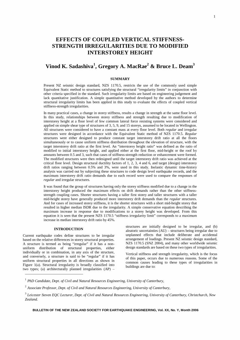
1
EFFECTS OF COUPLED VERTICAL STIFFNESS-STRENGTH IRREGULARITIES DUE TO MODIFIED
INTERSTOREY HEIGHT
Vinod K. Sadashiva1, Gregory A. MacRae2 & Bruce L. Deam3
SUMMARY
Present NZ seismic design standard, NZS 1170.5, restricts the use of the commonly used simple Equivalent Static method to structures satisfying the structural “irregularity limits” in conjunction with other criteria specified in the standard. Such irregularity limits are based on engineering judgement and lack quantitative justification. A simple quantitative method developed by the authors to determine structural irregularity limits has been applied in this study to evaluate the effects of coupled vertical stiffness-strength irregularities.
In many practical cases, a change in storey stiffness, results a change in strength at the same floor level. In this study, relationships between storey stiffness and strength resulting due to modification of interstorey height at a floor level of few common lateral force resisting systems were considered and applied on simple shear type of structures of 3, 5, 9, and 15 storeys, assumed to be located in Wellington. All structures were considered to have a constant mass at every floor level. Both regular and irregular structures were designed in accordance with the Equivalent Static method of NZS 1170.5. Regular structures were either designed to produce constant target interstorey drift ratio at all the floors simultaneously or to cause uniform stiffness distribution throughout the elevation of structure, with the target interstorey drift ratio at the first level. An “interstorey height ratio” was defined as the ratio of modified to initial interstorey height, and applied either at the first floor, mid-height or the roof by amounts between 0.5 and 3, such that cases of stiffness-strength reduction or enhancement were formed. The modified structures were then redesigned until the target interstorey drift ratio was achieved at the critical floor level. Design structural ductility factors of 1, 2, 3, 4 and 6, and target (design) interstorey drift ratios ranging between 0.5% and 3%, were used in this study. Inelastic dynamic time-history analysis was carried out by subjecting these structures to code design level earthquake records, and the maximum interstorey drift ratio demands due to each record were used to compare the responses of regular and irregular structures.
It was found that the group of structures having only the storey stiffness modified due to a change in the interstorey height produced the maximum effects on drift demands rather than the other stiffness-strength coupling cases. Shorter structures having a taller first storey and taller structures with a taller mid-height storey have generally produced more interstorey drift demands than the regular structures. And for cases of increased storey stiffness, it is the shorter structures with a short mid-height storey that resulted in higher median ISDR due to the irregularity. A simple conservative equation describing the maximum increase in response due to modifications to a storey height was developed. From this equation it is seen that the present NZS 1170.5 “stiffness irregularity limit” corresponds to a maximum increase in median interstorey drift ratio by 45%.
1 PhD Candidate, Dept. of Civil and Natural Resources Engineering, University of Canterbury, 2 Associate Professor, Dept. of Civil and Natural Resources Engineering, University of Canterbury, 3 Leicester Steven EQC Lecturer, Dept. of Civil and Natural Resources Engineering, University of Canterbury, Christchurch, New Zealand.
INTRODUCTION
Current earthquake codes define structures to be irregular based on the relative differences in storey structural properties. A structure is termed as being “irregular” if it has a non-uniform distribution of structural properties, either individually or in combination, in any axis of the structure, and conversely, a structure is said to be “regular” if it has uniform structural properties in all directions as shown in Figure 1(a). Structural irregularity is broadly classified into two types; (a) architecturally planned irregularities (AP) –
structures are initially designed to be irregular, and (b) aleatoric uncertainties (AU) – structures being irregular due to unplanned effects that include deliberate and accidental arrangement of loadings. Present NZ seismic design standard, NZS 1170.5 (SNZ 2004), and many other worldwide seismic design standards are based on these two types of irregularities.
Vertical stiffness and strength irregularity, which is the focus of this paper, occurs due to numerous reasons. Some of the common causes leading to these types of irregularities in buildings are due to:
BULLETIN OF THE NEW ZEALAND SOCIETY FOR EARTHQUAKE ENGINEERING, Vol. XX, No. Y, Month 2006
2
Difference in interstorey height at a particular floor level as compared to adjacent level, as shown in Figure 1(b);
Modification of member properties, member sizes, material, at a floor level, as shown in Figure 1(c);
Vertical discontinuities of structural members at a particular level as shown in Figure 1(c); or
Lack of infill material or open storey at a floor level as shown in Figure 1(d).
This paper addresses the effects of vertical stiffness-strength irregularities on the seismic response of structures by finding answers to the following questions:
1. How does NZS 1170.5 restrict the use of simple methods to analyse structures with stiffness-strength irregularity?
2. What past research on stiffness-strength irregularity has been conducted?
3. What stiffness-strength coupling is likely in realistic structures due to a modified storey height?
4. Which floor/floors are sensitive to a reduced stiffness only/and strength change due to a taller storey?
5. How do the responses differ when a storey’s height is decreased compared to other floors?
6. What level of increase in response due to stiffness-strength irregularity caused by a modified interstorey height does the current NZ seismic standard correspond to?
LIMITATION OF NZS 1170.5 EQUIVALENT STATIC METHOD TO CONSIDER STIFFNESS-STRENGTH
IRREGULARITY
Approximations to the exact response of a structure under the design level excitation may be obtained by carrying out numerous 3-D inelastic dynamic time history analyses (IDTHA) considering all relevant effects and using the best information available. Factors that should be considered include foundation effects, floor diaphragm effects, and the likely variation of earthquake demand and structural capacity.
In general, this type of approximate analysis is too complex for design engineers, so simpler, and hence more approximate analysis methods are commonly used. These approximate methods are calibrated based on the response of regular structures. However, when it is felt that a structure is too irregular, some approximate analysis methods are not permitted to be used. Many worldwide codes define structures to be irregular if they do not meet the “irregularity limits” laid in the codes. The need for simple methods for engineers to rapidly evaluate irregular structures has already been emphasized elsewhere (Sadashiva et al. 2009).
The common simple analysis method, Equivalent Static (ES) method is not permitted by NZS 1170.5 to be used for designing a structure if: (a) the height of the structure is more than 10m; (b) the fundamental natural period of the structure is more than 0.4s; and (c) the irregularity limits are not satisfied. The current NZ seismic standard (NZS 1170.5), like many other worldwide codes, specifies individual irregularity limits for structures with mass, stiffness, strength and plan irregularities that restrict the use of ES method. These irregularity limits are set to make designers aware of the existence of irregularities and the ill effects they produce when
Uniform structural properties in all directions
Different interstorey height
Difference in member material
Termination of column
No infill material
(a) “Regular” structure with uniform structural property in all directions.
(b) Excessive floor height at a particular floor level.
(c) Vertical discontinuity at a floor level or adjacent levels with dissimilar structural materials.
(d) Lack of infill material at a floor level.
Figure 1: Examples of vertical Stiffness-Strength irregularities.
3
a structure has irregularities (SEAOC blue book, 1999). Hence, these individual limits are based on engineering judgement and lack theoretical justification.
Stiffness-strength irregularity, the effects of which are investigated in this study, is said to exist by NZS 1170.5 (Cl. 4.5.1), when:
The lateral stiffness of a storey is less than 70% of the stiffness of any adjacent storey, or less than 80% of the average stiffness of the three storeys above or below in the structure.
The storey shear strength at a floor level is less than 90% that in the storey above.
Although separate irregularity limits are defined for stiffness and strength irregularity, in many practical scenarios, stiffness and strength vary together. For example, when cross-sectional property is changed at floor level, stiffness and strength at that storey are modified together. Hence, in this paper, stiffness and strength irregularities are combined together and their coupled effects on seismic demands are evaluated.
PREVIOUS RESEARCH ON VERTICAL STIFFNESS-STRENGTH IRREGULARITY
Very few researchers have attempted to investigate the effects of vertical structural irregularities on the seismic response of the structures. Those that have studied have not provided rational justification on the appropriateness of the irregularity limits specified in the NZS 1170.5 and other international codes with the same or similar criteria. An overview of earlier approaches and findings on stiffness-strength effects is summarised below. The stiffness-strength limits for regular buildings, as specified by the Uniform Building Code (UBC) were evaluated by Valmundsson and Nau (1997) by comparing the responses obtained due to time-history analysis using 4 unscaled earthquake records, and the ES method of UBC. Regular structures, represented by plane frames of 5, 10, and 20 storeys, with beams modelled to be stronger than the columns, were defined to have a constant floor mass at each floor level, and a uniform stiffness distribution required to achieve a series of 6 target fundamental periods for each structure height was calculated. First storey stiffness and/or strength of the regular structures were reduced by different amounts to form the irregular structures. A reduction in stiffness alone by 30% was shown to increase the drift by 30% and a decrease in maximum ductility demand by about 20%. Also, this effect on drift was found to decrease with the design ductility. It was found that the ductility demand increased for cases of only first storey strength reduction, and this increase was seen to increase with the structure height and decreased with the design ductility, especially for taller structures. Combined stiffness and strength irregularity cases were created by reducing first storey stiffness and strength proportionally. The ductility demand was found to increase significantly with the height of the building, and this increase was found to be less in case of higher design ductility’s. This study concluded that for a structure to be recognised as being “regular”, the first storey should be stronger than the storey above it.
Al-Ali and Krawinkler (1998) studied the effects of vertical irregularities on height-wise variations of seismic demands by conducting elastic and inelastic dynamic analyses (using 15 records) on 2-D single-bay 10-storey generic structures, assuming the columns to be weaker than the beams. Responses of structures with stiffness or/and strength irregularity were compared with the response of a reference structure that had a uniform distribution of mass over the height and an associated stiffness distribution that resulted in a straight-line first mode shape with storey stiffness’s tuned to
produce a first mode period of 3s when designed according to the modal superposition technique. Stiffness was reduced at the first level or at the mid-height by 0.1, 0.25, and 0.5 times the stiffness at the corresponding floor of the base structure. And, storey stiffness’s of the lower half of the structure was increased by amounts of 2, 4, and 10 times the stiffness at the respective floors of the base case. The stiffness distributions for all the cases were then tuned till the irregular structures had a fundamental period of 3s. Since stiffness irregularities change the distribution of elastic storey shear demands, storey strengths for each of the cases with stiffness irregularities were tuned to their own elastic storey shear distribution obtained from SRSS analyses using the National Earthquake Hazard Reduction Program (NEHRP) spectrum reduced by a strength reduction factor (3 and 6). Storey drift demands were found to increase in the “soft” storey and decrease in most of the other storeys, and the roof drift demands were seen to be less sensitive to the presence of stiffness irregularity. Strength irregularities were introduced by increasing the strength of a specific storey (or storeys) by 2 times the strength of the same storey in the reference base structure, rather than decreasing the storey strength. The stiffness and mass distributions were kept the same as for the base case. It was found that apart from the weak storey (or storeys) at upper half of structure; the roof drift demand did not change by large amounts due to the presence of vertical strength irregularity. Combined stiffness and strength irregularity was limited to cases with equal stiffness and strength modifications by two times the base case stiffness-strength distributions, and was applied at the first level, or the mid-height, or in the lower half of structures. The stiffness-strength distributions at the other floors were kept the same as for their individual irregularity cases. Cases with combined irregularities were shown to generally yield the same trend in responses as the cases with only strength irregularities, but with a larger magnitude.
Chintanapakdee and Chopra (2004) compared the seismic demands for vertically irregular and regular frames of 12 storey height, determined by non-linear response history analysis using a set of 15 earthquake records. For this study, a base case structure, modelled as a beam hinge model, was designed so that the stiffness distribution over the structure height produced equal drifts in all the storeys under the International Building Code (IBC) lateral forces. The target fundamental period was fixed at 2.4s. Numerous irregular frames were obtained by modifying the stiffness or/and strength of the base case by modification factors of 2 and 5. Irregularities were introduced at the first, or the mid-height, or the topmost level, or the lower half of the structure. Stiffness irregular cases were obtained by modifying the stiffness of the chosen irregular floor/floors and tuning the stiffness distribution till the target fundamental period of 2.4s was achieved. All storey strengths were uniformly scaled so that the irregular frames had the same yield base shear as the base case. Cases with only strength irregularity were created by modifying the storey strength of the chosen floor/floors and then uniformly tuning all storey strengths till the irregular frames achieved the same yield base shear as the base case. Combined cases of stiffness-strength irregularity were created by making equal modifications to both the stiffness and strength distributions as described for their individual cases. Like previous researchers, the effects of combined stiffness-strength irregularities were seen to be more influential than any other type of vertical irregularity. Soft and/or weak storey were found to increase the drift demands in the modified and neighbouring storeys, and decreased the drift demands at other storeys. Stiff and/or strong storey decreased the drift demands in the modified and neighbouring storeys and increased the drift demands in other storeys. Effects of an irregular storey on the drift demands in other storeys were strongly dependent on the storey location. These trends described differ from the results obtained from Al-Ali and Krawinkler (1998), where the
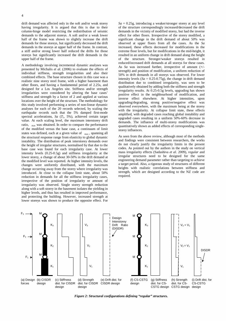
4
drift demand was affected only in the soft and/or weak storey having irregularity. It is argued that this is due to their column-hinge model restricting the redistribution of seismic demands to the adjacent storeys. A soft and/or a weak lower half of the frame was shown to slightly increase the drift demands for those storeys, but significantly decreased the drift demands in the storeys at upper half of the frame. In contrast, a stiff and/or strong lower half reduced the drifts for those storeys but significantly increased the drift demands in the upper half of the frame.
A methodology involving incremental dynamic analyses was presented by Michalis et al. (2006) to evaluate the effects of individual stiffness, strength irregularities and also their combined effects. The base structure chosen in this case was a realistic nine storey steel frame, with a higher basement than other floors, and having a fundamental period of 2.25s, and designed for a Los Angeles site. Stiffness and/or strength irregularities were considered by altering the base cases’ stiffness and strength by a factor of 2 and applied at various locations over the height of the structure. The methodology for this study involved performing a series of non-linear dynamic analyses for each of the 20 records selected, by scaling the earthquake records such that the 5% damped first-mode spectral accelerations, Sa (T1, 5%), achieved certain target value. At each scaling level, the maximum interstorey drift ratio, max was obtained. In order to compare the performance of the modified versus the base case, a continuum of limit states was defined, each at a given value of max , spanning all the structural response range from elasticity to global dynamic instability. The distribution of peak interstorey demands over the height of irregular structures, normalised by that due to the base case was found for each irregularity case. At lower intensity levels (0.25-0.5g) and stiffness irregularity at the lower storey, a change of about 30-50% in the drift demand at the modified level was reported. At higher intensity levels, the changes were uniformly distributed, with the maximum change occurring away from the storey where irregularity was introduced. At close to the collapse limit state, about 50% reduction in demands for all the stiffness irregularity cases, irrespective of the position of irregularity or amount of irregularity was observed. Single storey strength reduction along with a soft storey in the basement isolates the yielding in higher levels, and thus has resulted in improved performance, and protecting the building. However, increased strength at lower storeys was shown to produce the opposite effect. For
Sa = 0.25g, introducing a weaker/stronger storey at any level of the structure correspondingly increased/decreased the drift demands in the vicinity of modified storey, but had the inverse effect for other floors. Irrespective of the storey modified, a significant change in the drift demand of about 50% was observed at upper floors from all the cases. As the Sa increased, these effects decreased for modifications in the extreme floor levels, but for modifications in the mid-height, it resulted in an uniform change in drift demand along the height of the structure. Stronger/weaker storeys resulted in reduced/increased drift demands at all storeys for these cases. As Sa was increased further, irrespective of amount (+/- strength) and position of modification, a uniform reduction of 50% in drift demands in all storeys was observed. For lower intensity levels (Sa = 0.25-0.75g), the change in drift demand distribution due to combined irregularity, was seen to be qualitatively obtained by adding both the stiffness and strength irregularity results. At 0.25-0.5g levels, upgrading has shown positive effect in the neighbourhood of modification, and inverse effect elsewhere. At higher intensities, upon upgrading/degrading, strong positive/negative effect was observed everywhere, with the maximum being at the storey with the irregularity. At collapse limit state, these effects amplified, with degraded cases reaching global instability and upgraded cases resulting in a uniform 50%-60% decrease in demands. The influence of multi-storey modifications was quantitatively shown as added effects of corresponding single-storey influences.
As seen from the above review, although most of the methods and findings were consistent between researchers, the works do not clearly justify the irregularity limits in the present codes. As pointed out by the authors in the study on vertical mass irregularity effects (Sadashiva et al. 2009), regular and irregular structures need to be designed for the same engineering demand parameter rather than targeting to achieve a target period. Also, a rigorous study of structures of different heights with realistic correlations between stiffness and strength, which are designed according to the NZ code are required.
Figure 2: Structural configurations defining “regular” structures.
(a) Design forces
F3
F2
F1
V3
V2
V1
V3 = V1
V2 = V1
V1
Design Interstorey Drift Ratio (DISDR)
DISDR M
M
M
K3
K2
K1
(b) CISDR design
(c) Stiffness dist. for CISDR design
(d) Strength dist. for CISDR design
(e) Drift dist. for CISDR design
M
M
M
K3
K2
K1
(f) CS-CSTG design
(g) Stiffness dist. for CS-CSTG design
(h) Strength dist. for CS-CSTG design
(i) Drift dist. for CS-CSTG design
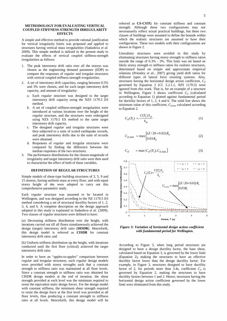
5
METHODOLOGY FOR EVALUATING VERTICAL COUPLED STIFFNESS-STRENGTH IRREGULARITY
EFFECTS
A simple and effective method to provide rational justification for vertical irregularity limits was proposed and applied to structures having vertical mass irregularities (Sadashiva et al. 2009). This simple method is utilised in the present study to evaluate the effects of vertical coupled stiffness-strength irregularities as follows:
1. The peak interstorey drift ratio over all the storeys was chosen as the engineering demand parameter (EDP) to compare the responses of regular and irregular structures with vertical coupled stiffness-strength irregularities.
2. A set of interstorey drift capacities, ranging between 0.5% and 3% were chosen, and for each target interstorey drift capacity, and amount of irregularity: a. Each regular structure was designed to the target
interstorey drift capacity using the NZS 1170.5 ES method.
b. A set of coupled stiffness-strength irregularities were introduced at various locations over the height of the regular structure, and the structures were redesigned using NZS 1170.5 ES method to the same target interstorey drift capacity.
c. The designed regular and irregular structures were then subjected to a suite of scaled earthquake records, and peak interstorey drifts due to the suite of records were obtained.
d. Responses of regular and irregular structures were compared by finding the difference between the median responses of the two structures.
3. The performance distributions for the chosen magnitude of irregularity and target interstorey drift ratio were then used to characterise the effect of both of these variables.
DEFINITION OF REGULAR STRUCTURES
Simple models of shear-type building structures of 3, 5, 9 and 15 storeys, having uniform mass at every floor, and with equal storey height of 4m were adopted to carry out this comprehensive parametric study.
Each regular structure was assumed to be located in Wellington, and was designed according to the NZ 1170.5 ES method considering a set of structural ductility factors of 1, 2, 3, 4, and 6. A complete description on the design approach adopted in this study is explained in Sadashiva et al. (2009). Two classes of regular structures were defined to have:
(a) Decreasing stiffness distribution over the height, with iterations carried out till all floors simultaneously achieved the design (target) interstorey drift ratio (DISDR). Henceforth, this design model is referred as CISDR for constant interstorey drift ratio; and
(b) Uniform stiffness distribution up the height, with iterations conducted until the first floor (critical) achieved the target interstorey drift ratio.
In order to have an “apples-to-apples” comparison between regular and irregular structures, each regular design models were provided with storey strengths such that a constant strength to stiffness ratio was maintained at all floor levels. Since a constant strength to stiffness ratio was obtained for CISDR design models at the end of iteration, the shear strength provided at each level was the minimum required to resist the equivalent static design forces. For the design model with constant stiffness, the minimum shear strength required to resist the design force at the first level was provided at all floor levels, thus producing a constant strength to stiffness ratio at all levels. Henceforth, this design model will be
referred as CS-CSTG for constant stiffness and constant strength. Although these two configurations may not necessasarily reflect actual practical buildings, but these two classes of buildings were assumed to define the bounds within which the realistic structures are assumed to have their configuration. These two models with their configurations are shown in Figure 2.
Unrealistic structures were avoided in this study by eliminating structures having storey strength to stiffness ratios outside the range of 0.3% - 3%. This limit was set based on likely storey strength to stiffness ratios for realistic structures, determined based on simple and approximate empirical relations (Priestley et al., 2007) giving yield drift ratios for different types of lateral force resisting systems. Also, structures having the horizontal design action coefficient, Cd governed by Equation 2 (Cl. 5.2.1.1, NZS 1170.5) were ignored from this work. That is, for an example of a structure in Wellington, Figure 3 shows coefficient Cd (calculated according to Equation 1) plotted against fundamental period for ductility factors of 1, 2, 4 and 6. The solid line shows the minimum value of this coefficient, Cd,min calculated according to Equation 2.
µkSTC
TC pd
)()( 1
1 = (1)
⎩⎨⎧ +
=u
ud R
RZC
03.0)02.020/(
maxmin, (2)
}{ min,1),(max ddd CTCC = (3)
According to Figure 3, when long period structures are designed to have a design ductility factor, the base shear, calculated based on Equation 3, is governed by the lower limit (Equation 2), making the structures to have an effective ductility factor lower than the design ductility factor. For example, in Figure 3, structures designed to have ductility factor of 2, for periods more than 3.4s, coefficient Cd is governed by Equation 2, making the structures to have ductility factors between 1 and 2. Hence, structures having the horizontal design action coefficient governed by the lower limit were eliminated from this study.
0
0.1
0.2
0.3
0.4
0.5
0.6
0.7
0.8
0 1 2 3 4 5
Period, T (s)
Hor
izon
tal D
esig
n A
ctio
n C
oeffi
cien
t, Cd(
T)
µ = 1 µ = 2
µ = 4 µ = 6
Figure 3: Variation of horizontal design action coefficient with fundamental period for Wellington.
⎩⎨⎧ +
=u
ud R
RZC
03.0)02.020/(
maxmin,
µkSTC
TC pd
)()( 1
1 =
6
CORRELATIONS BETWEEN STOREY STIFFNESS AND STRENGTH DUE TO RELATIVE DIFFERENCES
IN STOREY HEIGHT
In most practical scenarios, a change in stiffness is accompanied by a change in strength. Therefore, studying stiffness irregularity alone, or strength irregularity alone, while being interesting, does not represent the behaviour of actual structures. In this paper, the effects of coupled stiffness-strength irregularities, caused due to modified interstorey height at a floor level are investigated. Other member properties are assumed to remain unchanged and equal that of regular structures. A study on the effects of coupled stiffness-strength irregularities due to relative differences in member properties has been conducted and presented by Sadashiva et al. (2010).
A change in interstorey height from ho to hm results in a change in storey stiffness, and/no change in the corresponding storey strength. Relationships between the storey stiffness and strength due to a modified interstorey height can be obtained for various types of lateral-force-resisting (LFR) systems as given in Table 1. Here, the modified lateral stiffness at a chosen floor level for irregularity, Km, is given by Equation 4 as the product of the stiffness modification factor corresponding to the LFR system, k-LFR and the initial lateral stiffness at the chosen level, Ko. The corresponding storey strength can remain unchanged as seen in a steel shear wall, or vary proportionally with stiffness as seen for a braced frame or vary by differing amounts as for moment frames. Hence, similar to Equation 4, the modified storey strength at the level with modified interstorey height, hm, is given by Equation 5 as the product of strength modification factor corresponding to the LFR system, v-LFR and the initial storey strength provided for the floor level, Vo. Thus, a total of four groups with the above correlations between storey stiffness and strength are formed that define the types of irregular structures used to evaluate their coupled effects. In Equations 4 and 5, the modification factors are functions of the parameter interstorey height ratio, hrat, which is defined by Equation 6 as the ratio of modified interstorey height, hm to the initial interstorey height, ho.
oLFRkhm KK *−= β (4)
oLFRvhm VV *−= β (5)
⎟⎟⎠
⎞⎜⎜⎝
⎛=
o
mrat h
hh (6)
The sensitivity of the magnitude of coupled stiffness-strength irregularities on the response of structures were investigated by choosing a set of hrat that resulted in cases of stiffness reduction or enhancement at the floor with the modified interstorey height. For each hrat, the stiffness and strength modification factors were calculated and applied to obtain the modified properties. The modification factors used in this study, calculated for each group and for the set of hrat are tabulated in Table 2.

7
Lateral-force-resisting (LFR) system Modified storey stiffness, Khm Modified storey strength, Vhm
(a) Shear Wall – Group 1
h
δs F
L
hAGK s=
3ysA
Vσ
=
⎟⎟⎠
⎞⎜⎜⎝
⎛⎟⎟⎠
⎞⎜⎜⎝
⎛=
so
o
m
so
o
hmAG
hhAG
KK
*
om
ohm K
hh
K *⎟⎟⎠
⎞⎜⎜⎝
⎛=
orat
hm Kh
K *1⎟⎟⎠
⎞⎜⎜⎝
⎛=
okhm KK *1−= β
⎟⎟⎠
⎞⎜⎜⎝
⎛⎟⎟⎠
⎞⎜⎜⎝
⎛=
⎟⎠⎞⎜⎝
⎛
⎟⎠⎞⎜⎝
⎛
y
y
ooo
mhmhm
GG
hKV
hKV
σσ 3*
3
oo
m
o
hmhm V
hh
KK
V ** ⎟⎟⎠
⎞⎜⎜⎝
⎛⎟⎟⎠
⎞⎜⎜⎝
⎛=
ohm VV =
ovhm VV *1−= β
(b) Moment Frame (strong column weak beam mechanism) – Group 2
Mp
h
L
∆
F
26
hLIE
K = h
MV p=
⎟⎟⎠
⎞⎜⎜⎝
⎛⎟⎟⎠
⎞⎜⎜⎝
⎛=
o
o
m
o
o
hmIE
hLhL
IEK
K6
*6 2
2
om
ohm K
hh
K *2
⎟⎟⎠
⎞⎜⎜⎝
⎛=
orat
hm Kh
K *12
⎟⎟⎠
⎞⎜⎜⎝
⎛=
okhm KK *2−= β
1=⎟⎠⎞⎜⎝
⎛
⎟⎠⎞⎜⎝
⎛
ooo
mhmhm
hKV
hKV
oo
m
m
oo
o
m
o
hmhm V
hh
hh
Vhh
KK
V ****2
⎟⎟⎠
⎞⎜⎜⎝
⎛⎟⎟⎠
⎞⎜⎜⎝
⎛=⎟⎟⎠
⎞⎜⎜⎝
⎛⎟⎟⎠
⎞⎜⎜⎝
⎛=
orat
hm Vh
V *1⎟⎟⎠
⎞⎜⎜⎝
⎛=
ovhm VV *2−= β
(c) Moment Frame (strong beam weak column mechanism) – Group 3
F
h
Mp
L
312
hIE
K = hM
V p2=
⎟⎟⎠
⎞⎜⎜⎝
⎛⎟⎟⎠
⎞⎜⎜⎝
⎛=
o
o
m
o
o
hmIE
hh
IEK
K12
*12 3
3
om
ohm K
hh
K *3
⎟⎟⎠
⎞⎜⎜⎝
⎛=
orat
hm Kh
K *13
⎟⎟⎠
⎞⎜⎜⎝
⎛=
okhm KK *3−= β
⎟⎟⎠
⎞⎜⎜⎝
⎛=
⎟⎠⎞⎜⎝
⎛
⎟⎠⎞⎜⎝
⎛
o
m
ooo
mhmhm
hh
hKV
hKV
oo
m
m
oo
o
m
o
hmhm V
hh
hh
Vhh
KK
V ****232
⎟⎟⎠
⎞⎜⎜⎝
⎛⎟⎟⎠
⎞⎜⎜⎝
⎛=⎟⎟⎠
⎞⎜⎜⎝
⎛⎟⎟⎠
⎞⎜⎜⎝
⎛=
orat
hm Vh
V *1⎟⎟⎠
⎞⎜⎜⎝
⎛=
ovhm VV *3−= β
(d) Braced Frame – Group 4
δx
δa
Ha
F
h
L
θ
22 hL
EAK a
+=
22 hL
LAV yaa
+=
σ
⎟⎟⎟
⎠
⎞
⎜⎜⎜
⎝
⎛ +
⎟⎟⎟
⎠
⎞
⎜⎜⎜
⎝
⎛
+=
EAhL
hL
EAK
K
ao
o
m
ao
o
hm22
22*
om
ohm K
hL
hLK *
22
22
⎟⎟⎟
⎠
⎞
⎜⎜⎜
⎝
⎛
+
+=
( ) oorat
ohm K
hhL
hLK *
* 22
22
⎟⎟⎟
⎠
⎞
⎜⎜⎜
⎝
⎛
+
+=
okhm KK *4−= β
⎟⎟⎠
⎞⎜⎜⎝
⎛⎟⎟⎠
⎞⎜⎜⎝
⎛=
⎟⎠⎞⎜⎝
⎛
⎟⎠⎞⎜⎝
⎛
Lh
hL
hKV
hKV
y
o
m
y
ooo
mhmhm
εε
*
oo
hmhm V
KK
V *⎟⎟⎠
⎞⎜⎜⎝
⎛=
( ) oorat
ohm V
hhL
hLV *
* 22
22
⎟⎟⎟
⎠
⎞
⎜⎜⎜
⎝
⎛
+
+=
ovhm VV *4−= β
Table 1: Correlations between storey stiffness-strength due to modified interstorey height.
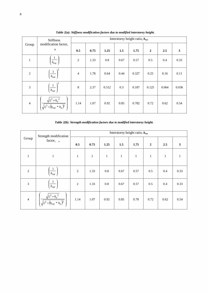
8
Interstorey height ratio, hrat Group
Stiffness modification factor,
k
0.5
0.75
1.25
1.5
1.75
2
2.5
3
1 ⎟⎟⎠
⎞⎜⎜⎝
⎛
rath1 2 1.33 0.8 0.67 0.57 0.5 0.4 0.33
2 2
1⎟⎟⎠
⎞⎜⎜⎝
⎛
rath 4 1.78 0.64 0.44 0.327 0.25 0.16 0.11
3 3
1⎟⎟⎠
⎞⎜⎜⎝
⎛
rath 8 2.37 0.512 0.3 0.187 0.125 0.064 0.036
4 ( ) ⎟⎟⎟
⎠
⎞
⎜⎜⎜
⎝
⎛
+
+22
22
* orat
o
hhL
hL 1.14 1.07 0.92 0.85 0.782 0.72 0.62 0.54
Interstorey height ratio, hrat Group Strength modification
factor, v
0.5
0.75
1.25
1.5
1.75
2
2.5
3
1 1 1 1 1 1 1 1 1
1
2 ⎟⎟⎠
⎞⎜⎜⎝
⎛
rath1 2 1.33 0.8 0.67 0.57 0.5 0.4 0.33
3 ⎟⎟⎠
⎞⎜⎜⎝
⎛
rath1 2 1.33 0.8 0.67 0.57 0.5 0.4 0.33
4 ( ) ⎟⎟⎟
⎠
⎞
⎜⎜⎜
⎝
⎛
+
+22
22
* orat
o
hhL
hL 1.14 1.07 0.92 0.85 0.78 0.72 0.62 0.54
Table 2(a): Stiffness modification factors due to modified interstorey height.
Table 2(b): Strength modification factors due to modified interstorey height.

9
APPLYING COUPLED STIFFNESS AND STRENGTH IRREGULARITIES
The effect of coupled stiffness-strength over the height of the structures was conducted by applying the irregularities either at the first level, or at the mid-height, or at the topmost floor level of regular structures. This was done by modifying the interstorey height by hrat at the chosen floor level for irregularity, and by introducing the stiffness modification factor at the same level. The modified structure was then redesigned until the target interstorey drift ratio was achieved at the critical floor level. For example, as shown in Figure 4, consider a regular 3 storey CS-CSTG structure designed for a structural ductility factor of 4, and having stiffness distribution resulting in a target interstorey drift ratio (DISDR) of 1% at the first floor level. If it is intended to have a soft storey at the third floor, the interstorey height of the third level is modified by hrat and the storey stiffness of the regular structure at that level is reduced by means of stiffness modification factor, k, by an amount corresponding to the hrat and the group of LFR system. Upon making this change in storey stiffness, the critical floor would no longer have the chosen DISDR. In order to compare the responses of regular and irregular structures, all storey stiffness are then uniformly scaled by a scaling factor, , and the irregular structure is redesigned till the chosen DISDR is achieved at the critical floor. Since all storey stiffness’s are uniformly scaled, at the end of iteration, the irregular structure would still maintain the applied k at the chosen floor level, which is third floor in this example. However, the relative storey stiffness’s at other floors remain unchanged and equal the corresponding storey stiffness’s of regular structure. The storey strength distribution is similarly modified at the chosen floor level according to Equation 5, and uniformly scaled with factor.
STRUCTURAL MODELLING AND ANALYSIS
Earlier studies (e.g., MacRae et al. 2004, Tagawa et al. 2006) on structural modelling have shown that frames modelled as a combination of vertical shear beam and a vertical flexural column (labelled as SFB in Figure 5) can represent the behaviour of real structures well. If the flexural beam is not considered, unrealistically high drift concentrations may occur. The flexural beam represents all continuous columns throughout the whole structure. The flexural beam stiffness ratio, cc, in actual structure tends to be greater than 0.5, so this value at all levels was used in all analyses. EI was computed for the flexural beam from the equation in Figure 5. Sadashiva et al. (2009) have also shown that regular
structures modelled without the flexural beam have increased median interstorey drift demands. This increase in demand was observed to increase with the height of the structure, and about 50% increase in median interstorey drift demand was observed for 9 storey structures.
Figure 5: Combined vertical Shear and Flexural Beam (SFB model).
A set of 20 SAC (SEAOC-ATC-CUREE) earthquake ground motion records for Los Angeles, with probabilities of exceedance of 10% in 50 years, were used for the ground motion suite. Response spectra were developed for each of the selected records and the accelerations within each record were scaled so that its single-degree-of-freedom elastic displacement response spectrum matched the design interstorey drift for NZS 1170.5 in the city chosen. Here, both the structural ductility factor and structural performance factor were unity.
Rayleigh damping has commonly been adopted to represent damping effects within multi-degree-of-freedom structures for several decades. A recent study by Sadashiva et al. (2009) on the effects of different types of Rayleigh damping models show that the differences in drift responses due to three types of Rayleigh damping models available in RUAUMOKO (Carr 2004) time-history program were minimal. However, the tangent stiffness proportional Rayleigh damping model that uses the absolute form of equation of motion was considered to be more appropriate than other types of Rayleigh damping, to be used in IDTHA. Such a damping model that considers the non-linearity effects of structures, also assures that the damping forces go to zero at the end of excitation, and hence it has been used for all IDTHA conducted in this work. In order to avoid super-critical damping or negative damping, the first mode and the mode corresponding to number of storeys in the structure (Carr 2004) were nominated as the two modes with 5% of critical damping. The RUAUMOKO computer program was used to carry out all the IDTHA considering a post elastic stiffness (bilinear) factor of 1%.
Interpretation of Inelastic Dynamic Time-History Analysis Results
The peak interstorey drift ratio (ISDR) at every floor level, and within the structure, when subjected to each of the 20 earthquake records, was obtained. It was assumed that the distribution of ISDR is lognormal (Cornell et al. 2002), so the median and dispersion were found to measure the likely and the spread in the results respectively, as per Equations 7 and 8.
( )⎟⎟
⎠
⎞⎜⎜
⎝
⎛∑
==
n
iix
nex 1
ln1
ˆ (7)
( )∑=
−−
=n
iix xx
n1
2ln ˆlnln
)1(1σ (8)
where xi = peak interstorey drift ratio due to ith record; and
n = total number of earthquake records considered.
∆n
∆2
∆1
∆n-1
Rigid Link
Pin
Shear-Beam Flexural-Beam
∆n
∆2
∆1
∆n-1
Rigid Link
Pin
Shear-Beam Flexural-Beam
oii
icci
KH
IE3=α
where αcci = continuous column stiffness ratio at level, i;E = elastic modulus;Ii = moment of inertia at the ith level;
Hi = storey height of the ith level; andKoi = lateral initial stiffness of the ith level.
∆n
∆2
∆1
∆n-1
Rigid Link
Pin
Shear-Beam Flexural-Beam
∆n
∆2
∆1
∆n-1
Rigid Link
Pin
Shear-Beam Flexural-Beam
oii
icci
KH
IE3=α
where αcci = continuous column stiffness ratio at level, i;E = elastic modulus;Ii = moment of inertia at the ith level;
Hi = storey height of the ith level; andKoi = lateral initial stiffness of the ith level.
Ko
Ko
Ko
ho
ho
F3
F2
F1
Km = k-1 Ko hm
ho
ho
Ko
Ko
Km = k-1 Ko hm
ho
ho
Ko
Ko
(a) Design forces
(b) Regular CS-CSTG design with DISDR at first floor
(c) Introducing stiffness modification at third floor
(d) Irregular structure with DISDR at critical floor
Figure 4: Stiffness irregularity introduced by modifying the interstorey height for CS-CSTG design.
10
Comparison between regular and irregular structures – effect of magnitude and location of modified interstorey height ratio: The median of peak interstorey drift ratio (ISDR) obtained for each irregular structure has been compared with the corresponding ISDR of regular structure. The change in median ISDR due to the presence of coupled stiffness-strength irregularity has been used to show the effects of irregularity in the following section. The response plot labels in the following figures have the format “N-L (Q)”, where N refers to the number of storeys in the structure, L refers to the location (floor level) of the irregularity and Q defines the magnitude of interstorey height ratio, hrat. Many designs for Groups 2-4 structures were eliminated due to having unrealistic storey strength to stiffness ratios and/or not satisfying the condition related to the base shear calculation as explained earlier. Also, some of the response plots shown in Figures 6 and 7 for Group 1 structures, designed for structural ductility factor of 3 have limited results due these two conditions imposed in the design.
Effect of increased interstorey height and reduced storey stiffness: The response plots for Group 1 CISDR and CS-CSTG designs are shown in Figures 6(a) and 6(b) respectively for cases of increase in interstorey height at the chosen irregular floor level. Figure 6(a) shows that for all DISDR’s when the first storey of 3 storeys and the mid-height storey of taller structures were increased by hrat of 1.5, the median ISDR’s increased over the regular structures’ responses. The maximum median ISDR increase due to this magnitude of hrat and the corresponding decreased stiffness at the first floor was 28%, 1.5%, and 1.7% respectively for 3, 9, and 15 storey structures. An increased storey height at the mid-height of 3 storey structures than other structure heights have shown to increase the median ISDR’s. The maximum increase in ISDR was 10% for 3 storeys and about 6% for 9 and 15 storey irregular structures. For all DISDR’s, a taller storey at the topmost floor for all structures has produced lesser drifts than the regular structures. On average, decrease in median ISDR due to irregularity at the roof was 7%, 4%, and 3% for 3, 9, and 15 storey structures respectively. As the interstorey height ratio was increased from 1.5 to a maximum of 3, the 3 storey structures performed better than the regular ones, and for taller structures, a slight increase in the median ISDR along with the hrat was observed. Nine storey structures with hrat = 3 applied at the mid-height produced the maximum increase in median ISDR of 13%, and the maximum decrease in median ISDR of 26% was obtained for 3 storey structures having this hrat at the roof.
Figure 6(b) show that for Group 1 CS-CSTG designs, an increase in the first floor height by hrat = 1.5 produced a maximum increase in median ISDR of 37% for 3 storey structures, whereas for taller structures, the median ISDR decreased due to this hrat by about 4%. The increase in storey height of the topmost level rather than the mid-height was seen to be more significant for 3 storey structures with DISDR = 0.5%, producing a maximum of 16% increase in the median ISDR over the regular structure, and for taller structures this increase in median ISDR was less than 2.5% for the same hrat and DISDR. The responses of CS-CSTG designs were more sensitive to an increase in hrat than for CISDR designs. That is, the median ISDR due to an increased storey height at the first level for 3 storey structures was 40% and for taller structures the responses closely matched with the corresponding regular structures. But an increased storey height and reduced stiffness at the mid-height was more significant than irregularity at the roof, producing respectively a maximum increase in median
ISDR of 26%, 13%, and 4% for 3, 9, and 15 storey irregular structures.
Effect of decreased interstorey height and increased storey stiffness: The effect of decreased interstorey height for Group 1 CISDR designs is shown in Figure 7(a). For hrat = 0.75 at the first floor and irrespective of the structure height the regular structures have median ISDR more than the irregular ones. It is the decreased storey height of the mid-height level for 3 storey and topmost storey for taller structures that has produced increased drifts over the regular structure. For hrat = 0.75 at the mid-height of 3 storey structure, a maximum increase in median ISDR of 7%, and an average decrease of 3% for taller structures was observed. The maximum increases in median ISDR due to a shorter topmost level decreased with the structure height, and were 6%, 3%, and 2% respectively for 3, 9, and 15 storey irregular structures. The above effects were again seen for hrat = 0.5, however with slightly higher magnitude.
In case of Group 1 CS-CSTG designs, as seen in Figure 7(b), the mid-height of 3 storey structure and the first floor of taller structures with hrat = 0.75 produces higher drift demands due to irregularity than the other two floor levels chosen for irregularity. A maximum increase in median ISDR due to this hrat at the first floor for 3 storey structures was 17%, and its magnitude decreased with the structure height. About 5% and 3% increase in median ISDR’s for 9 and 15 storey structures were respectively obtained. For hrat = 0.75 at the mid-height, the increase in median ISDR was 22% for 3 storey structures and less than 2% for 9 and 15 storey irregular structures. Irregularity at the roof has shown to be insignificant for all structure heights, and the responses closely matched with the responses of regular structures. Again, the above observations were generally the same when hrat was decreased from 0.75 to 0.5.

11
0 0 .5 1 1.5 2 2.5 30
0 .5
1
1 .5
2
2 .5
3
Design Interstorey Drift Ratio (%)
Med
ian
Inte
rsto
rey
Drift
Rat
io (%
)
3 -1(1.5)3 -2(1.5)3 -3(1.5)DISDRRegular
0 0.5 1 1.5 2 2.5 3
0
0.5
1
1.5
2
2.5
3
Design Interstorey Drift Ratio (%)M
edia
n In
ters
tore
y D
rift R
atio
(%) 9-1(1.5)
9-5(1.5)9-9(1.5)DISDRRegular
0 0.5 1 1.5 2 2.5 3
0
0.5
1
1.5
2
2.5
3
Design Interstorey Drift Ratio (%)
Med
ian
Inte
rsto
rey
Drif
t Rat
io (%
) 15-1(1.5)15-8(1.5)15-15(1.5)DISDRRegular
0 0.5 1 1.5 2 2.5 3
0
0.5
1
1.5
2
2.5
3
Design Interstorey Drift Ratio (%)
Med
ian
Inte
rsto
rey
Drif
t Rat
io (%
) 3-1(2)3-2(2)3-3(2)DISDRRegular
0 0.5 1 1.5 2 2.5 3
0
0.5
1
1.5
2
2.5
3
Design Interstorey Drift Ratio (%)
Med
ian
Inte
rsto
rey
Drif
t Rat
io (%
)
9-1(2)9-5(2)9-9(2)DISDRRegular
0 0.5 1 1.5 2 2.5 3
0
0.5
1
1.5
2
2.5
3
Design Interstorey Drift Ratio (%)M
edia
n In
ters
tore
y D
rift R
atio
(%) 15-1(2)
15-8(2)15-15(2)DISDRRegular
0 0.5 1 1.5 2 2.5 30
0.5
1
1.5
2
2.5
3
Design Interstorey Drift Ratio (%)
Med
ian
Inte
rsto
rey
Drif
t Rat
io (%
) 3-1(2.5)3-2(2.5)3-3(2.5)DISDRRegular
0 0.5 1 1.5 2 2.5 3
0
0.5
1
1.5
2
2.5
3
Design Interstorey Drift Ratio (%)
Med
ian
Inte
rsto
rey
Drif
t Rat
io (%
)
9-1(2.5)9-5(2.5)9-9(2.5)DISDRRegular
0 0.5 1 1.5 2 2.5 3
0
0.5
1
1.5
2
2.5
3
Design Interstorey Drift Ratio (%)
Med
ian
Inte
rsto
rey
Drif
t Rat
io (%
)
15-1(2.5)15-8(2.5)15-15(2.5)DISDRRegular
0 0.5 1 1.5 2 2.5 30
0.5
1
1.5
2
2.5
3
Design Interstorey Drift Ratio (%)
Med
ian
Inte
rsto
rey
Drif
t Rat
io (%
) 3-1(3)3-2(3)3-3(3)DISDRRegular
0 0.5 1 1.5 2 2.5 3
0
0.5
1
1.5
2
2.5
3
Design Interstorey Drift Ratio (%)
Med
ian
Inte
rsto
rey
Drif
t Rat
io (%
)
9-1(3)9-5(3)9-9(3)DISDRRegular
0 0.5 1 1.5 2 2.5 3
0
0.5
1
1.5
2
2.5
3
Design Interstorey Drift Ratio (%)
Med
ian
Inte
rsto
rey
Drif
t Rat
io (%
)
15-1(3)15-8(3)15-15(3)DISDRRegular
(1) hrat = 1.5
(2) hrat = 2
(3) hrat = 2.5
(4) hrat = 3
Figure 6(a): Effect of decreased interstorey height for Group 1 structures - CISDR design ( = 3, Z = 0.4).
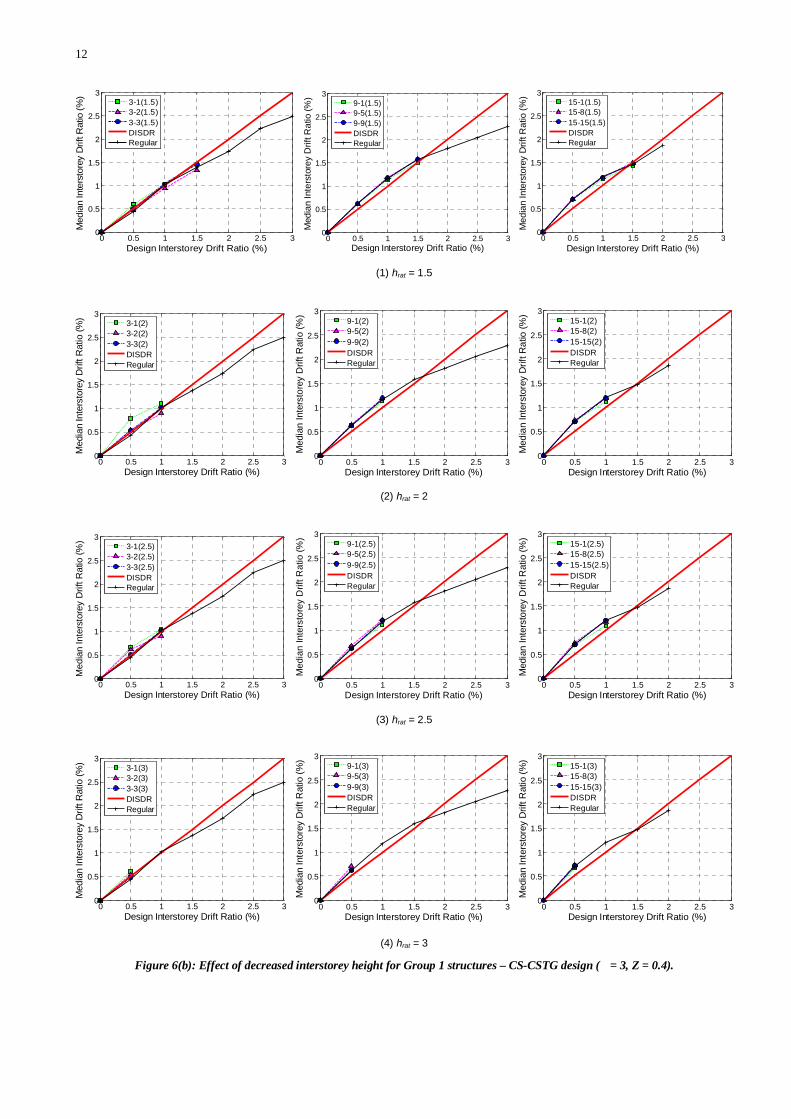
12
0 0.5 1 1.5 2 2.5 30
0.5
1
1.5
2
2.5
3
Design Interstorey Drift Ratio (%)
Med
ian
Inte
rsto
rey
Drif
t Rat
io (%
)
3-1(1.5)3-2(1.5)3-3(1.5)DISDRRegular
0 0.5 1 1.5 2 2.5 3
0
0.5
1
1.5
2
2.5
3
Design Interstorey Drift Ratio (%)
Med
ian
Inte
rsto
rey
Drif
t Rat
io (%
)
9-1(1.5)9-5(1.5)9-9(1.5)DISDRRegular
0 0.5 1 1.5 2 2.5 3
0
0.5
1
1.5
2
2.5
3
Design Interstorey Drift Ratio (%)
Med
ian
Inte
rsto
rey
Drif
t Rat
io (%
)
15-1(1.5)15-8(1.5)15-15(1.5)DISDRRegular
0 0.5 1 1.5 2 2.5 30
0.5
1
1.5
2
2.5
3
Design Interstorey Drift Ratio (%)
Med
ian
Inte
rsto
rey
Drif
t Rat
io (%
) 3-1(2)3-2(2)3-3(2)DISDRRegular
0 0.5 1 1.5 2 2.5 3
0
0.5
1
1.5
2
2.5
3
Design Interstorey Drift Ratio (%)
Med
ian
Inte
rsto
rey
Drif
t Rat
io (%
)
9-1(2)9-5(2)9-9(2)DISDRRegular
0 0.5 1 1.5 2 2.5 3
0
0.5
1
1.5
2
2.5
3
Design Interstorey Drift Ratio (%)
Med
ian
Inte
rsto
rey
Drif
t Rat
io (%
)
15-1(2)15-8(2)15-15(2)DISDRRegular
0 0.5 1 1.5 2 2.5 30
0.5
1
1.5
2
2.5
3
Design Interstorey Drift Ratio (%)
Med
ian
Inte
rsto
rey
Drif
t Rat
io (%
)
3-1(2.5)3-2(2.5)3-3(2.5)DISDRRegular
0 0.5 1 1.5 2 2.5 3
0
0.5
1
1.5
2
2.5
3
Design Interstorey Drift Ratio (%)
Med
ian
Inte
rsto
rey
Drif
t Rat
io (%
)
9-1(2.5)9-5(2.5)9-9(2.5)DISDRRegular
0 0.5 1 1.5 2 2.5 3
0
0.5
1
1.5
2
2.5
3
Design Interstorey Drift Ratio (%)
Med
ian
Inte
rsto
rey
Drif
t Rat
io (%
)
15-1(2.5)15-8(2.5)15-15(2.5)DISDRRegular
0 0.5 1 1.5 2 2.5 30
0.5
1
1.5
2
2.5
3
Design Interstorey Drift Ratio (%)
Med
ian
Inte
rsto
rey
Drif
t Rat
io (%
) 3-1(3)3-2(3)3-3(3)DISDRRegular
0 0.5 1 1.5 2 2.5 3
0
0.5
1
1.5
2
2.5
3
Design Interstorey Drift Ratio (%)
Med
ian
Inte
rsto
rey
Drif
t Rat
io (%
)
9-1(3)9-5(3)9-9(3)DISDRRegular
0 0.5 1 1.5 2 2.5 3
0
0.5
1
1.5
2
2.5
3
Design Interstorey Drift Ratio (%)
Med
ian
Inte
rsto
rey
Drif
t Rat
io (%
)
15-1(3)15-8(3)15-15(3)DISDRRegular
(1) hrat = 1.5
(2) hrat = 2
(3) hrat = 2.5
(4) hrat = 3
Figure 6(b): Effect of decreased interstorey height for Group 1 structures – CS-CSTG design ( = 3, Z = 0.4).

13
Determination of Irregularity Limit: For each model designed for a structural ductility factor, the maximum median interstorey drift for each interstorey height ratio, hrat, was determined as follows:
Step 1. For each structure height with hrat at the chosen irregularity position, compute the maximum increase in median ISDR from all DISDR’s;
Step 2. Repeat Step 1 for all the three positions chosen for applying coupled stiffness-strength irregularity;
Step 3. Compute the maximum of median ISDR’s obtained from Step 2;
Step 4. Repeat Step 3 for all structure heights considered in this study;
Step 5. Compute the maximum of median ISDR’s obtained from Step 4;
Figure 8 shows the maximum increase in median ISDR plotted against the hrat for all coupled stiffness-strength irregularity cases considered in this study. The figure shows that the group of structures having a storey modified by hrat that results in only a corresponding storey stiffness change produces the largest effects due to irregularity than other groups. Also, the figures show that generally the structures designed to have a uniform distribution of stiffness and strength (CS-CSTG) have produced greater increases in median ISDR due to hrat than the structures designed to produce equal floor drifts (CISDR). However, the response plots of CISDR and CS-CSTG irregular structures have shown that the former type of structures in many cases have produced larger median ISDR’s than the CS structures. Similar observations were seen in the study of mass irregularity effects (Sadashiva et al. 2009).
Simple equations for determining the mass irregularity limits (Sadashiva et al. 2009) and coupled stiffness-strength
irregularity limits due to relative differences in storey member properties (Sadashiva et al. 2010) were developed. On similar lines, Equation 9 is developed for Group 1 structures having either a short or a taller storey at the critical floor producing the maximum increase in median ISDR.
( )1100 1 −= −kIRR β (9)
where IRR is the Irregular response greater than the regular response; and k-1 is the stiffness modification factor for Group 1 structures.
This conservative equation can then be used to estimate the likely increase in response due to modifications to a storey height. For example, according to Figure 9, if it is not intended to have responses to be more than 20% due to modifications in a storey height, then the modified height of a storey cannot be less than 0.85 or more than 1.2 times the regular storey height. Figure 9 also shows that the NZS 1170.5 stiffness irregularity limit of 0.7 corresponds to an increase in median ISDR of about 45%.
0 0.5 1 1.5 2 2.5 3
0
0.5
1
1.5
2
2.5
3
Design Interstorey Drift Ratio (%)
Med
ian
Inte
rsto
rey
Drif
t Rat
io (%
)
3-1(0.75)3-2(0.75)3-3(0.75)DISDRRegular
0 0.5 1 1.5 2 2.5 3
0
0.5
1
1.5
2
2.5
3
Design Interstorey Drift Ratio (%)
Med
ian
Inte
rsto
rey
Drif
t Rat
io (%
)
9-1(0.75)9-5(0.75)9-9(0.75)DISDRRegular
0 0.5 1 1.5 2 2.5 3
0
0.5
1
1.5
2
2.5
3
Design Interstorey Drift Ratio (%)
Med
ian
Inte
rsto
rey
Drif
t Rat
io (%
)
15-1(0.75)15-8(0.75)15-15(0.75)DISDRRegular
0 0.5 1 1.5 2 2.5 3
0
0.5
1
1.5
2
2.5
3
Design Interstorey Drift Ratio (%)
Med
ian
Inte
rsto
rey
Drif
t Rat
io (%
)
3-1(0.75)3-2(0.75)3-3(0.75)DISDRRegular
0 0.5 1 1.5 2 2.5 3
0
0.5
1
1.5
2
2.5
3
Design Interstorey Drift Ratio (%)
Med
ian
Inte
rsto
rey
Drif
t Rat
io (%
)9-1(0.75)9-5(0.75)9-9(0.75)DISDRRegular
0 0.5 1 1.5 2 2.5 3
0
0.5
1
1.5
2
2.5
3
Design Interstorey Drift Ratio (%)
Med
ian
Inte
rsto
rey
Drif
t Rat
io (%
)
15-1(0.75)15-8(0.75)15-15(0.75)DISDRRegular
(a) CISDR design - k = 0.75
(b) CS-CSTG design - k = 0.75
Figure 7: Effect of increased interstorey height for Group 1 structures ( = 3, Z = 0.4).
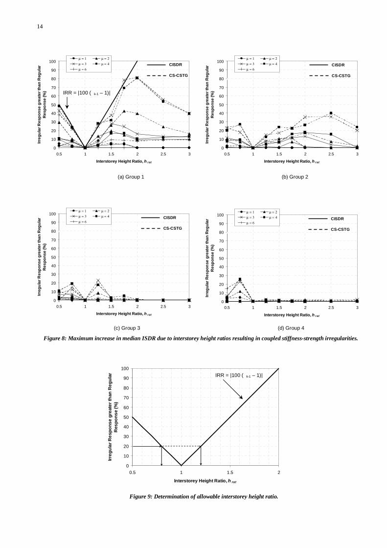
14
0
10
20
30
40
50
60
70
80
90
100
0.5 1 1.5 2 2.5 3
Interstorey Height Ratio, h rat
Irreg
ular
Res
pons
e gr
eate
r tha
n R
egul
ar
Res
pons
e (%
)
µ = 1 µ = 2µ = 3 µ = 4µ = 6
CISDR
CS-CSTG
IRR = |100 ( k-1 – 1)|
0
10
20
30
40
50
60
70
80
90
100
0.5 1 1.5 2 2.5 3
Interstorey Height Ratio, h rat
Irreg
ular
Res
pons
e gr
eate
r tha
n R
egul
ar
Res
pons
e (%
)
µ = 1 µ = 2µ = 3 µ = 4µ = 6
CISDR
CS-CSTG
0
10
20
30
40
50
60
70
80
90
100
0.5 1 1.5 2 2.5 3
Interstorey Height Ratio, h rat
Irreg
ular
Res
pons
e gr
eate
r tha
n R
egul
ar
Res
pons
e (%
)
µ = 1 µ = 2µ = 3 µ = 4µ = 6
CISDR
CS-CSTG
0
10
20
30
40
50
60
70
80
90
100
0.5 1 1.5 2 2.5 3
Interstorey Height Ratio, h rat
Irreg
ular
Res
pons
e gr
eate
r tha
n R
egul
ar
Res
pons
e (%
)µ = 1 µ = 2µ = 3 µ = 4µ = 6
CISDR
CS-CSTG
0
10
20
30
40
50
60
70
80
90
100
0.5 1 1.5 2
Interstorey Height Ratio, h rat
Irreg
ular
Res
pons
e gr
eate
r tha
n R
egul
ar
Res
pons
e (%
)
IRR = |100 ( k-1 – 1)|
Figure 9: Determination of allowable interstorey height ratio.
(c) Group 3 (d) Group 4
Figure 8: Maximum increase in median ISDR due to interstorey height ratios resulting in coupled stiffness-strength irregularities.
(a) Group 1 (b) Group 2
15
CONCLUSIONS
The effects of coupled vertical stiffness-strength irregularities caused in structures due to a short or a tall storey were evaluated and presented in this paper. Regular structures, represented by shear-type structures of 3, 5, 9, and 15 storeys having equal storey height, assumed to be in Wellington and having a constant floor mass at every floor level were designed for a range of structural ductility factors of 1, 2, 3, 4, and 6 according to the NZS ES method. The stiffness distribution over the height was either provided such that it resulted in design (target) interstorey drift ratios (DISDR) at all floors simultaneously or a uniform stiffness distribution that produced DISDR at the first level was provided. The strength distribution over the height was provided such that the strength to stiffness ratio at each floor was constant. All structures having the base shear governed by the lower limit of the code design spectra and with unrealistic storey strengths to stiffness ratios were eliminated from this study. An “interstorey height ratio” was defined as the ratio of modified to initial interstorey height, and applied either at the first floor, mid-height or the roof. A corresponding modification to the storey stiffness and/or strength due to a change in the storey height was introduced at the chosen floor and the structures were then redesigned until the critical floor/floors achieved the target DISDR. The change in the median of peak interstorey drift ratios (ISDR), due to coupled stiffness-strength irregularities, obtained from inelastic dynamic time-history analysis were then used to explain the effects of coupled stiffness-strength irregularity. The conclusions derived from this study can be summarised as below:
1. Simple analysis methods such as the NZS 1170.5 Equivalent Static (ES) method, is not allowed to be used to design structures if the storey stiffness is less than 70% of any adjacent floor, and the storey strength is less than 90% of the storey above. Such “irregularity limits” in the design code are based on engineering judgement, to show the designers the adverse effects of irregularities. A systematic quantitative justification for these limits is not available and it is not clear what level of irregularity corresponds to what change in response;
2. Effects of vertical stiffness-strength irregularities are evaluated in this paper from a design perspective. That is, the drift demands for regular and irregular structures are compared by designing both types of structures to the same target interstorey drift ratio, rather than tuning the structures to have a target period, as adopted by some previous researchers. By comparing the responses of the regular and irregular structures, relationships between structural irregularity and the change in response may be obtained;
3. Realistic correlations between storey stiffness and strength due to modifications to a storey height for a few common lateral force resisting systems were determined. A range of interstorey height ratios that produced cases of stiffness-strength reduction or enhancement were selected to investigate the effects of magnitude of irregularities;
4. Many designs were eliminated due to not satisfying the condition imposed on the base shear calculation and for not having realistic storey strength to stiffness ratios. The group of structures having only the storey stiffness modified due to a change in storey height at a floor level (Group 1 structures) produced the maximum adverse effects of irregularity. For this group with CISDR or CS-CSTG configuration, a taller first storey for short period structures and a taller mid-height storey for taller structures, were found to produce median ISDR’s greater than the regular structures. The increase in median ISDR due to irregularity generally reduced with the structure height;
5. For Group 1 structures, the effects of enhanced storey stiffness due to a short storey were less than those due to reduced storey stiffness cases. A shorter floor at the mid-height of short period CISDR and CS-CSTG designs generally tended to produce higher increases in median ISDR’s due to irregularity than other irregularity positions and structure heights; and
6. A simple conservative equation that would facilitate the designers to rapidly estimate the likely increase in median ISDR due to a modified storey height was developed. From the equation, it is seen that the present NZS 1170.5 “irregularity limit” for stiffness irregularity correspond to an increase in median ISDR of about 45%.
ACKNOWLEDGEMENTS
This research work, which is a part of the project on irregularity effects, is sponsored by the New Zealand Earthquake commission (www.eqc.govt.nz). The authors would like to thank this organisation for their financial support.
REFERENCES
1 Al-Ali, A. A. K., and Krawinkler, H. (1998) “Effects of vertical irregularities on seismic behaviour of building structures”. Department of Civil and Environmental Engineering, Stanford University, San Francisco. Report No. 130.
2 Carr, A. J. (2004) “Ruaumoko 2D – Inelastic dynamic analysis”. Department of Civil Engineering, University of Canterbury, Christchurch.
3 Chintanapakdee, C., and Chopra, A. K. (2004) “Seismic response of vertically irregular frames: Response history and modal pushover analyses”. Journal of Structural Engineering. 130 (8): 1177-1185.
4 Cornell, C. A., Fatemeh, J. F., Hamburger, R. O., and Foutch, D. A. (2002) “Probabilistic basis for 2000 SAC FEMA steel moment frame guidelines”. Journal of Structural Engineering. 128 (4): 526-533.
5 MacRae, G. A., Kimura, Y., and Roeder, C. W. (2004) “Effect of column stiffness on braced frame seismic behaviour”. Journal of Structural Engineering. 130 (3): 381-391.
6 Michalis, F., Vamvatsikos, D., and Monolis, P. (2006) “Evaluation of the influence of vertical irregularities on the seismic performance of a nine-storey steel frame”. Earthquake Engineering and Structural Dynamics. 35: 1489-1509.
7 Sadashiva, V. K., MacRae, G. A., and Deam, B. L. (2009) “Determination of structural irregularity limits – mass irregularity example”. Bulletin of the New Zealand Society for Earthquake Engineering. (submitted - March 2009).
8 Sadashiva, V. K., MacRae, G. A., and Deam, B. L. (2010) “Seismic response of structures with coupled vertical stiffness-strength irregularities”. Bulletin of the New Zealand Society for Earthquake Engineering. (submitted - June 2009).
9 SNZ. (2004) “NZS 1170.5 Supp 1:2004, Structural Design Actions. Part 5: Earthquake actions – New Zealand – Commentary”. Standards New Zealand, Wellington.
10 SEAOC. (1999) “Recommended Lateral Force Requirements and Commentary”. Seismology Committee,

16
Structural Engineers Association of California. Seventh Edition.
11 Tagawa, H., MacRae, G. A., and Lowes, L. N. (2006) “Evaluation of simplification of 2D moment frame to 1D MDOF coupled shear-flexural-beam model”. Journal of Structural & Constructional Engineering. (Transactions of AIG), No. 609.
10 Valmundsson, E. V., and Nau, J. M. (1997) “Seismic response of building frames with vertical structural irregularities”. Journal of Structural Engineering. 123 (1): 30-41.

CHAPTER 5. TORSIONAL IRREGULARITY IN SINGLE STOREY STRUCTURES

1
M J
M J
∆y,wall1
Wall 2
Wall 1
Wall 1
Wall 2
(b) Deformation after Wall 1 yields (a) Translational Response at yield
N
∆i,cm
∆i,wall1
TORSIONALLY IRREGULAR SINGLE STORY STRUCTURE SEISMIC RESPONSE
Eu Ving Au1, Gregory MacRae1, Didier Pettinga2, Bruce Deam1 and Vinod Sadashiva1
SUMMARY
Impulse ground motions are applied to single story structures with different in-plane wall strength and stiffness, rotational inertia, and out-of-plane wall stiffness to obtain the dynamic response considering torsion. A simple algorithm giving results consistent with the impulse response is developed. It is shown that the median increase in response of the critical component considering torsion from earthquake records is similar to that from impulse records. Using this information, a simple design methodology is proposed which enables the likely critical element earthquake response considering torsion to be obtained from building analyses not considering torsion. Lastly, a design example is provided.
1 Department of Civil Engineering, University of Canterbury, Christchurch, New Zealand 2 Glotman•Simpson Consulting Engineers, 1661 West 5th Avenue, Vancouver, BC V6J 1N5, Canada
1. INTRODUCTION
For elastic structures, torsion is caused by stiffness eccentricities relative to the centre of mass. Such an eccentricity occurs from differences in stiffness between lateral-force resisting elements [1]. There is a significant body of research on the asymmetric response of these structures which has been summarised by Rutenburg [2] and De Stefano and Pintucchi [3].
For yielding structures, such as those which are subject to strong earthquake motions, torsional deformations may be accentuated by strength eccentricities. In Figure 1(a), a plan of a structure with constant stiffness in both in-plane walls and the mass centroid at the centre of the structure is shown. Before yielding occurs, both walls have the same deformation due to north-south translational shaking. If Wall 1 is weaker than Wall 2, then deformation at Wall 1 is likely to be significantly greater than that at Wall 2, as shown in Figure 1(b). This torsional effect must be considered to correctly evaluate wall demands for design. Methods to estimate the torsional effect are therefore required.
Figure 1: Inelastic Torsional Mechanism
Perhaps the most simple and easily applied concept for estimating torsional response in yielding structures was developed by Paulay [4]. If the structure has no out-of-plane walls (i.e. it is a torsionally unrestrained system), the wall behaviour is elastic perfectly plastic, and the rotational inertia
effects are ignored, then Paulay assumed that the displacement of the centre of mass was the same irrespective of whether or not torsion occurred. That is, when yielding occurs in the weakest wall (i.e. Wall 1 in Figure 1(b)), Wall 2 stops moving at the yield displacement of Wall 1, ∆y,wall1. At the peak response, the centre of mass has a total displacement, ∆u,cm, which is equal to the inelastic deflection, ∆i,cm, plus ∆y,wall1. Because the structure is symmetric, the total displacement of the critical wall, ∆u,crit, is given by Equation 1 as a result of geometric considerations.
cmiwallycritu ,1,, 2∆+∆=∆ (1)
For more general cases, where the in-plane walls have different stiffness and the centre of mass is not at the centre of the structure, the response of the structure could be estimated by first ignoring torsion to give ∆u,cm, and then using a static push through the centre of mass considering torsion to the same displacement, ∆u,cm, to finally obtain ∆u,crit.
While Paulay’s concept is simple, it does not consider the dynamic effect of rotational inertia, or out-of-plane walls. Paulay [5, 6] showed by means of dynamic inelastic time history analysis with rotational inertia effects included, that the rotational inertia reduces the propensity for twist about the vertical axis. It was also shown that the time of peak rotation in the structure was often not the same as that of the peak displacement in the critical element. Further investigation by Castillo [7] followed the concepts of Paulay, resulting in the recommendation that the centre of strength, rather than the centre of stiffness, as commonly used in earlier studies, should be as close as possible to the centre of mass.
Similar findings were published by Myslimaj and Tso [8], where the focus was on achieving a stable (or limited) torsional response through explicit design to locate the centres of strength and stiffness evenly either side of the centre of mass. While the emphasis is on strength here, these authors have argued that in real structures strength is often proportional to stiffness. Therefore, by satisfying the strength criteria, the stiffness criteria is also satisfied. In these cases, the
BULLETIN OF THE NEW ZEALAND SOCIETY FOR EARTHQUAKE ENGINEERING, Vol. ???????
(a) At Yield (b) After Wall 1 Yield
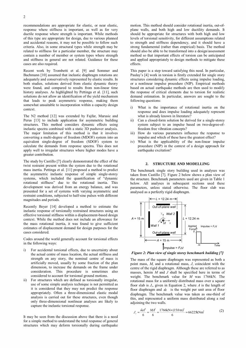
2
A = 15 m L = 12.24 m x
y
Wall 1
Wall 2
M J
Out-of-plane wall
Out-of-plane wall
Impulse = Fi∆t
Fi
∆t
Applied Force
Time
Impulse = Fi∆t
L = 12.24 m
A = 15 m
recommendations are appropriate for elastic, or near elastic, response where stiffness is important, as well as for very ductile response where strength is important. While methods of this type are appropriate for design, due to various planned and accidental reasons, it may not be possible to follow such criteria. Also, in some structural types while strength may be related to stiffness for a particular member, the structure may contain a number of member or system types where strength and stiffness in general are not related. Guidance for these cases are also required.
Recent work by Trombetti et al. [9] and Sommer and Bachmann [10] assumed that inelastic diaphragm rotations are adequately and conservatively represented by elastic results. In both studies, solutions derived from elastic dynamic theory were found, and compared to results from non-linear time history analyses. As highlighted by Pettinga et al. [11], such solutions do not allow an identification of the yield mechanism that leads to peak asymmetric response, making them somewhat unsuitable to incorporation within a capacity design context.
The N2 method [12] was extended by Fajfar, Marusic and Perus [13] to include application for asymmetric building structures. This method considers dynamic effects using inelastic spectra combined with a static 3D pushover analysis. The major limitation of this method is that it involves converting a multi-degree of freedom (MDOF) system into an equivalent single-degree of freedom (SDOF) system to calculate the demands from response spectra. This does not apply well to irregular structures where higher modes have a greater contribution.
The study by Castillo [7] clearly demonstrated the effect of the twist restraint present within the system due to the rotational mass inertia. Pettinga et al. [11] proposed a method to predict the asymmetric inelastic response of simple single-storey systems, which included the quantification of “dynamic rotational stiffness” due to the rotational inertia. This development was derived from an energy balance, and was presented for a set of systems with varying asymmetric and restraint conditions, subjected to half-sine pulses with different magnitudes and periods.
Recently Beyer [14] developed a method to estimate the inelastic response of torsionally restrained structures using an effective torsional stiffness within a displacement-based design context. While the method does not include an allowance for the mass rotational inertia, it was found to give sufficient estimates of displacement demand for design purposes for the cases considered.
Codes around the world generally account for torsional effects in the following ways:
i) For accidental torsional effects, due to uncertainty about the actual centre of mass location, the actual stiffness and strength on any story, the nominal centre of mass is artificially moved, usually by some fraction of the plan dimension, to increase the demands on the frame under consideration. This procedure is sometimes also considered to account for torsional ground motions.
ii) For structures which are defined as torsionally irregular, use of some simple analysis technique is not permitted as it is considered that they may not predict the response appropriately. Often a three-dimensional elastic modal analysis is carried out for these structures, even though only three-dimensional nonlinear analyses are likely to capture the inelastic torsional response.
It may be seen from the discussion above that there is a need for a simple method to understand the total response of general structures which may deform torsionally during earthquake
motion. This method should consider rotational inertia, out-of-plane walls, and both high and low ductility demands. It should be appropriate for structures with both high and low levels of torsional sensitivity, for different assumptions related to strength and stiffness dependency, and it should have a strong fundamental (rather than empirical) basis. The method should also be able to be transformed into a design/assessment method so that important effects of torsion can be anticipated and applied appropriately to design methods to mitigate these effects.
This paper is a step toward satisfying this need. In particular, Paulay’s [4] work in torsion is firstly extended for single story structures considering dynamic effects using impulse loading, or a nonlinear impulse procedure (NIP). Empirical methods based on actual earthquake methods are then used to modify the response of critical elements due to torsion for realistic demand estimation. In particular, answers are sought to the following questions:
i) What is the importance of rotational inertia on the response and does impulse loading adequately represent what is already known in literature?
ii) Can a closed-form solution be derived for a single-storey system subject to an impulse based on two-degree-of-freedom free vibration concepts?
iii) How do various parameters influence the response to impulse and which of these have the greatest effect?
iv) What is the applicability of the non-linear impulse procedure (NIP) in the context of a design approach for earthquake excitation?
2. STRUCTURE AND MODELLING
The benchmark single story building used in analyses was taken from Castillo [7]. Figure 2 below shows a plan view of the structure. Benchmark parameters used are given in Table 1 below. All analyses in subsequent sections used these parameters, unless stated otherwise. The floor slab was analysed as a perfectly rigid diaphragm.
Figure 2: Plan view of single storey benchmark building [7]
The mass of the square diaphragm was represented as both a point mass, M, and a rotational mass, J, coincident with the centre of the rigid diaphragm. Although these are referred to as masses, herein M and J shall be specified here in terms of weight. The benchmark value for M was 1766kN. The rotational mass for a uniformly distributed mass over a square floor slab is Jr, given in Equation 2, where A is the length of floor diaphragm and m̂ is the weight per unit area of floor diaphragm. The benchmark value was taken as one-third of this, and represented a uniform mass distributed along a rod adjoining the two walls.
2224
kNm 662256
m) 0.15(kN 176666
ˆ=×=== MAAmJr
(2)
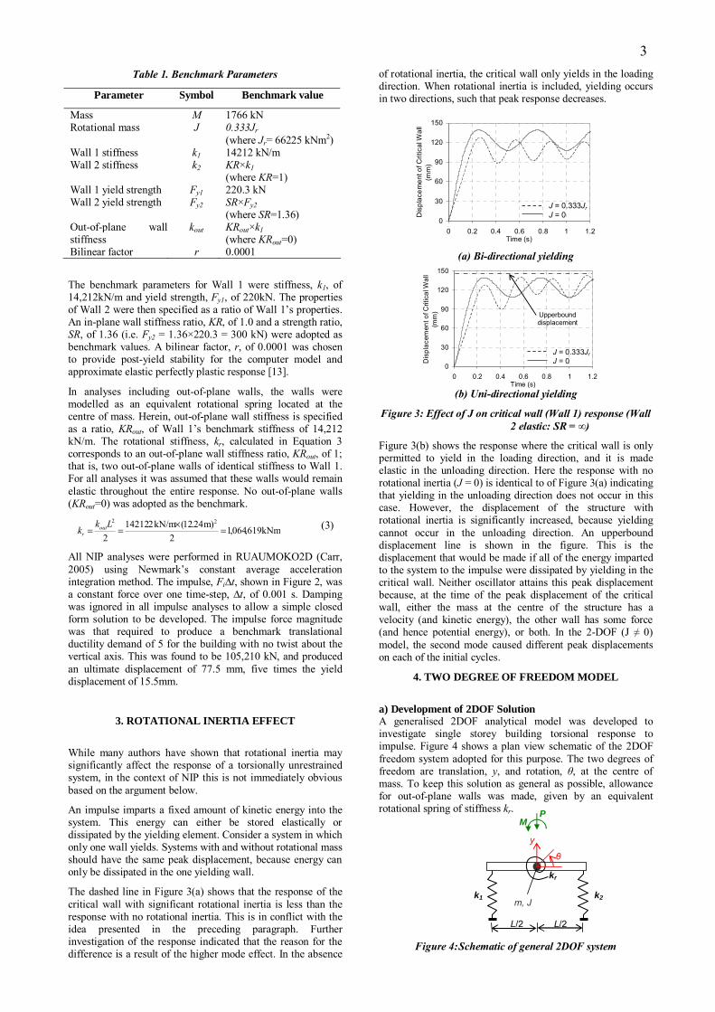
3
0
30
60
90
120
150
0 0.2 0.4 0.6 0.8 1 1.2Time (s)
Dis
plac
emen
t of C
ritic
al W
all
(mm
)
J = 0.333Jr J = 0
0
30
60
90
120
150
0 0.2 0.4 0.6 0.8 1 1.2Time (s)
Dis
plac
emen
t of C
ritic
al W
all
(mm
)
J = 0.333Jr J = 0
Upperbound displacement
P
m, J k1 k2
kr
M
y
θ
L/2 L/2
Table 1. Benchmark Parameters
Parameter Symbol Benchmark value
Mass M 1766 kN Rotational mass J 0.333Jr
(where Jr= 66225 kNm2) Wall 1 stiffness k1 14212 kN/m Wall 2 stiffness k2 KR×k1
(where KR=1) Wall 1 yield strength Fy1 220.3 kN Wall 2 yield strength Fy2 SR×Fy2
(where SR=1.36) Out-of-plane wall stiffness
kout KRout×k1 (where KRout=0)
Bilinear factor r 0.0001
The benchmark parameters for Wall 1 were stiffness, k1, of 14,212kN/m and yield strength, Fy1, of 220kN. The properties of Wall 2 were then specified as a ratio of Wall 1’s properties. An in-plane wall stiffness ratio, KR, of 1.0 and a strength ratio, SR, of 1.36 (i.e. Fy2 = 1.36×220.3 = 300 kN) were adopted as benchmark values. A bilinear factor, r, of 0.0001 was chosen to provide post-yield stability for the computer model and approximate elastic perfectly plastic response [13].
In analyses including out-of-plane walls, the walls were modelled as an equivalent rotational spring located at the centre of mass. Herein, out-of-plane wall stiffness is specified as a ratio, KRout, of Wall 1’s benchmark stiffness of 14,212 kN/m. The rotational stiffness, kr, calculated in Equation 3 corresponds to an out-of-plane wall stiffness ratio, KRout, of 1; that is, two out-of-plane walls of identical stiffness to Wall 1. For all analyses it was assumed that these walls would remain elastic throughout the entire response. No out-of-plane walls (KRout=0) was adopted as the benchmark.
kNm 619,064,12
)m 24.12( kN/m 2.142122
22
=×
==Lk
k outr
(3)
All NIP analyses were performed in RUAUMOKO2D (Carr, 2005) using Newmark’s constant average acceleration integration method. The impulse, Fi∆t, shown in Figure 2, was a constant force over one time-step, ∆t, of 0.001 s. Damping was ignored in all impulse analyses to allow a simple closed form solution to be developed. The impulse force magnitude was that required to produce a benchmark translational ductility demand of 5 for the building with no twist about the vertical axis. This was found to be 105,210 kN, and produced an ultimate displacement of 77.5 mm, five times the yield displacement of 15.5mm.
3. ROTATIONAL INERTIA EFFECT
While many authors have shown that rotational inertia may significantly affect the response of a torsionally unrestrained system, in the context of NIP this is not immediately obvious based on the argument below.
An impulse imparts a fixed amount of kinetic energy into the system. This energy can either be stored elastically or dissipated by the yielding element. Consider a system in which only one wall yields. Systems with and without rotational mass should have the same peak displacement, because energy can only be dissipated in the one yielding wall.
The dashed line in Figure 3(a) shows that the response of the critical wall with significant rotational inertia is less than the response with no rotational inertia. This is in conflict with the idea presented in the preceding paragraph. Further investigation of the response indicated that the reason for the difference is a result of the higher mode effect. In the absence
of rotational inertia, the critical wall only yields in the loading direction. When rotational inertia is included, yielding occurs in two directions, such that peak response decreases.
(a) Bi-directional yielding
(b) Uni-directional yielding
Figure 3: Effect of J on critical wall (Wall 1) response (Wall 2 elastic: SR = ∞)
Figure 3(b) shows the response where the critical wall is only permitted to yield in the loading direction, and it is made elastic in the unloading direction. Here the response with no rotational inertia (J = 0) is identical to of Figure 3(a) indicating that yielding in the unloading direction does not occur in this case. However, the displacement of the structure with rotational inertia is significantly increased, because yielding cannot occur in the unloading direction. An upperbound displacement line is shown in the figure. This is the displacement that would be made if all of the energy imparted to the system to the impulse were dissipated by yielding in the critical wall. Neither oscillator attains this peak displacement because, at the time of the peak displacement of the critical wall, either the mass at the centre of the structure has a velocity (and kinetic energy), the other wall has some force (and hence potential energy), or both. In the 2-DOF (J ≠ 0) model, the second mode caused different peak displacements on each of the initial cycles.
4. TWO DEGREE OF FREEDOM MODEL
a) Development of 2DOF Solution A generalised 2DOF analytical model was developed to investigate single storey building torsional response to impulse. Figure 4 shows a plan view schematic of the 2DOF freedom system adopted for this purpose. The two degrees of freedom are translation, y, and rotation, θ, at the centre of mass. To keep this solution as general as possible, allowance for out-of-plane walls was made, given by an equivalent rotational spring of stiffness kr.
Figure 4: Schematic of general 2DOF system
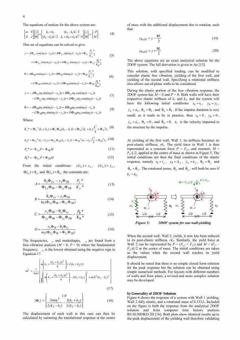
4
The equations of motion for the above system are:
⎭⎬⎫
⎩⎨⎧−
=⎭⎬⎫
⎩⎨⎧
θ⎥⎦
⎤⎢⎣
⎡++−
−++
⎭⎬⎫
⎩⎨⎧θ⎥
⎦
⎤⎢⎣
⎡MPy
LkkkLkkLkkkky
Jm
r 4/)(2/)(2/)(
00
22112
1221 (4)
This set of equations can be solved to give:
**))(sin())(cos(
**
))(sin())(cos(
2022022
1011011
θ
θΦ+−ωΦ+−ωΦ+
Φ+−ωΦ+−ωΦ=
KPttDttC
KP
ttBttAy
yyy
y
yyyy (5)
**
))(sin())(cos(
**
))(sin())(cos(
22222
11111
θ
θθθθ
θθθ
Φ+−ωΦ+−ωΦ+
Φ+−ωΦ+−ωΦ=θ
KP
ttDttC
KP
ttBttA
oo
y
yoo (6)
))(cos())(sin(
))(cos())(sin(
222222
111111
oyoy
oyoy
ttDttC
ttBttAy
−ωωΦ+−ωωΦ−
−ωωΦ+−ωωΦ−= (7)
))(cos())(sin(
))(cos())(sin(
222222
111111
oo
oottDttC
ttBttA−ωωΦ+−ωωΦ−
−ωωΦ+−ωωΦ−=θ
θθ
θθ (8)
Where:
ryyy kLkkLkkkkK 2
1
2
212
11211212
1 4)()()(* θθθ Φ++Φ+−ΦΦ++Φ= (9)
ryy kLkkLkkkkK 2
2
2
212
21222212
2 4)()()(* θθθθ Φ++Φ+−ΦΦ++Φ= (10)
MPP yy θΦ+Φ−= 11* (11)
MPP y θθ Φ+Φ−= 22* (12)
From the initial conditions: oo yty =)( , oo yty =)( ,
oot θ=θ )( and oot θ=θ )( , the constants are:
**
2112
22
y
y
yy
oyo
KPy
A −ΦΦ−ΦΦ
Φ−Φθ=
θθ
θ (13)
)( 21121
22
θθ
θ
ΦΦ−ΦΦωΦ−Φθ
=yy
oyo yB (14)
**
2112
11
θ
θ
θθ
θ −ΦΦ−ΦΦ
Φθ−Φ=
KPy
Cyy
yoo (15)
)( 21122
11
θθ
θ
ΦΦ−ΦΦωΦθ−Φ
=yy
yooyD (16)
The frequencies, i, and modeshapes, i, are found from a free-vibration analysis (M = 0, P = 0) where the fundamental frequency, 1, is the lowest obtained using the negative sign in Equation 17.
⎥⎥⎥⎥⎥⎥⎥
⎦
⎤
⎢⎢⎢⎢⎢⎢⎢
⎣
⎡
−+⎟⎟
⎠
⎞⎜⎜
⎝
⎛+−⎟
⎟⎠
⎞⎜⎜⎝
⎛ ++
±++⎟⎟⎠
⎞⎜⎜⎝
⎛ ++
=ω2
122
2
21
221
21
221
2
)()(4
)(
)(4
)(
21
kkmJLkkJLkkkm
kkJLkk
km
mJr
r
(17)
⎪⎭
⎪⎬⎫
⎪⎩
⎪⎨⎧
−+
−−ω=Φ
)()(2
)(2
0.1}{
12
21
12
2
kkLkk
kkLm ii (18)
The displacement of each wall in this case can then be calculated by summing the translational response at the centre
of mass with the additional displacement due to rotation, such that:
21LyyWall
θ−= (19)
22LyyWall
θ+= (20)
The above equations are an exact analytical solution for the 2DOF system. The full derivation is given in Au [15].
This solution, with specified loading, can be modified to consider elastic free vibration, yielding of the first wall, and yielding of the second wall. Specifying a rotational stiffness also allows out-of-plane walls to be considered.
During the elastic portion of the free vibration response, the 2DOF system has M = 0 and P = 0. Both walls will have their respective elastic stiffness of k1 and k2, and the system will have the following initial conditions: 10 tt = , 10 yy = ,
1uyo = , 1θ=θo , and 1θ=θo . If the impulse duration is very small, as it tends to be in practice, then 00 =t , 00 =y ,
io uy = , 0=θo , and 0=θo . iu is the velocity imparted to the structure by the impulse.
At yielding of the first wall, Wall 1, its stiffness becomes its post-elastic stiffness, rk1. The yield force in Wall 1 is then represented as a constant force P = Fy1, and moment, M = Fy1L/2, applied at the centre of mass as shown in Figure 5. The initial conditions are then the final conditions of the elastic response, namely ytt =0 , yy ∆=0 , yo uy = , yo θ=θ and
yo θ=θ . The rotational terms, oθ and oθ , will both be zero if k1 = k2.
P = Fy1
M, J rk1 k2
kr
M = Fy1L/2
y
θ
L/2 L/2
M, J rk1 k2
kr
y
θ
L/2 L/2
Fy1
Figure 5: 2DOF system for one-wall-yielding
When the second wall, Wall 2, yields, it now has been reduced to its post-elastic stiffness, rk2. Similarly, the yield force at Wall 2 can be represented by P = (Fy1 + Fy2) and M = (Fy1 - Fy2)L/2 at the centre of mass. The initial conditions are taken as the values when the second wall reaches its yield displacement.
It should be noted that there is no simple closed form solution for the peak response but the solution can be obtained using simple numerical methods. For layouts with different numbers of walls and floor plans, a revised and more complex solution may be developed.
b) Generality of 2DOF Solution Figure 6 shows the response of a system with Wall 1 yielding, Wall 2 fully elastic, and a rotational mass of 0.333Jr. Included on the figure is both the response from the analytical 2DOF solution and from computer time history analysis RUAUMOKO-2D [16]. Both plots show identical results up to the peak displacement of the yielding wall therefore validating

5 the 2DOF solution. Later, the two results begin to deviate because the equations developed do not consider unloading after yield, however this does not affect the predicted peak wall displacement.
-40
0
40
80
120
160
0 0.1 0.2 0.3 0.4 0.5
Time (s)
Dis
plac
emen
t (m
m)
Ruaumoko 2DOF solution
Wall 1
Wall 2
Centre of mass
Figure 6: Displacement response with one yielding wall
(Wall 2 elastic: SR= ∞ )
Figure 7 shows the response when the second wall is given a strength ratio of 1.36 and is allowed to yield. It shows that the second wall reaches its peak displacement before Wall 1 and that the 2DOF solution is valid up until this point. However, because the peak displacement of Wall 1 occurs after this, its peak response is not predicted well by the 2DOF solution because Wall 2 is unloading and this is not captured in the simple analytical solution. In this case, the peak displacement is overestimated by 12%. The 2DOF solution would therefore be conservative for design.
-50
0
50
100
150
0 0.1 0.2 0.3 0.4 0.5
Time (s)
Dis
plac
emen
t (m
m)
Ruaumoko 2DOF solution
Wall 1
Wall 2
Centre of mass
Figure 7: Displacement response with two walls
yielding
When out-of-plane walls are included in the analysis, the 2DOF solution gives a better approximation of the peak response of both walls. This is shown in Figure 8, where again a strength ratio of 1.36 is used and Wall 2 reaches its peak displacement first. The figure shows that for systems with sufficiently high out-of-plane wall stiffness the peak displacement of Wall 1 can also be predicted reasonably accurately.
0
20
40
60
80
100
120
0 0.1 0.2 0.3 0.4 0.5Time (s)
Dis
plac
emen
t of W
all1
(mm
) Ruaumoko 2DOF solution KRout=0
KRout=0.07
KRout=0.28
KRout=1.00
Figure 8: Critical wall displacement with two walls
yielding and out-of-plane walls
For an out-of-plane wall stiffness equal to Wall 1’s stiffness (KRout=1) the approximation is independent of the wall strength ratio as shown in Figure 9. That is, the 2DOF solution will still give reasonable predictions for both walls (Au, 2007).
0
10
20
30
40
50
60
70
80
0 0.1 0.2 0.3 0.4 0.5Time (s)
Dis
plac
emen
t of W
all1
(mm
)
Ruaumoko 2DOF solution
SR=1.00
SR=1.36
SR=1.82
SR=2.27
Figure 9: Critical wall displacement with two walls
yielding and out-of-plane walls (KRout=1.0)
c) Solution Stability The solution was found to become unstable when the strength and stiffness of both walls were identical and when rotational mass is zero – effectively resulting in a SDOF system. While the second degree of freedom could be condensed out, a rotational mass of 1 kNm2 and a 0.01 kN/m difference in wall stiffness was found to produce stability without loss of accuracy.
SENSITIVITY ANALYSIS
The benchmark structure given in Table 1 was used for all sensitivity studies, with one parameter changed at a time.
a) Effect of Rotational Mass While a greater rotational mass, J, causes a decrease in the displacement of the centre of mass, it does not always cause a reduction in the critical wall displacement as shown in Figure 10. Here, for unrealistically low values of rotational mass, the demand increases. However in general, increasing J decreases the demands and has a significant impact on the response of buildings with no out-of-plane walls.

6
0
30
60
90
120
150
0 0.05 0.1 0.15 0.2 0.25 0.3Time (s)
Dis
plac
emen
t of W
all1
(mm
) J=0 J=0.151Jr J=0.333Jr J=Jr J=1.21Jr J=1.51Jr
Figure 10: Sensitivity to J (Wall 2 elastic: SR= ∞ ) (KRout=1.0)
b) Effect of Out-of-Plane Wall Stiffness Figure 11 shows the response of a structure with Wall 1 yielding, Wall 2 fully elastic, a rotational mass of 0.333Jr and with out-of-plane walls of varying stiffness. The out-of-plane wall stiffness has little effect on the centre of mass displacement, but there is a considerable reduction in peak displacement of the critical wall. In addition, the peak critical wall displacement is reached earlier. The reason for this has been described by many authors in the past. It is that out-of-plane walls provide a resisting couple to the twist action; and provided they remain elastic, they are relatively stiff. Therefore, out-of-plane walls provide an effective method for limiting demands on the critical wall.
0
20
40
60
80
100
120
140
0 0.05 0.1 0.15 0.2 0.25 0.3Time (s)
Dis
plac
emen
t of W
all1
(mm
)
KRout=0.00 KRout=0.352 KRout=0.704 KRout=1.06 KRout=1.41
Figure 11: Sensitivity to out-of-plane wall stiffness (Wall
2 elastic: SR= ∞ )
c) Effect of Wall Strength Difference Figure 12 shows that by increasing the strength of Wall 2, a greater torsional response is obtained. That is, unwisely adding strength to a system can be harmful. Thus designers can minimise torsion in structures, undergoing significant yielding, by seeking to reduce strength differences between eccentric lateral-force resisting elements. This is consistent with Paulay’s concept of locating the centre of strength as close as possible to the centre of mass [6].
0
20
40
60
80
100
120
140
0 0.1 0.2 0.3 0.4 0.5Time (s)
Dis
plac
emen
t of W
all1
(mm
) SR=1.0 SR=1.2 SR=1.4 SR=1.8 SR=2.3
Figure 12: Sensitivity to in-plane wall strength difference
d) Effect of Rotational Mass with Out-of-Plane Walls Figure 13 shows the impulse time history response for a system with out-of-plane walls, for various rotational masses. Out-of-plane wall stiffness was taken as 7106.1 kN/m, which was half the in-plane wall stiffness (KRout=0.5). It may be seen that rotational inertia only has a minor affect on the response and if the out-of-plane wall stiffness is sufficiently high, rotational mass can be ignored.
0
20
40
60
80
100
0 0.1 0.2 0.3 0.4 0.5Time (s)
Dis
plac
emen
t of W
all1
(mm
)
J=0 J=0.151Jr J=0.333Jr J=Jr J=1.21Jr
Figure 13: Sensitivity to rotational inertia with out-of-
plane walls (KRout = 0.5)
EARTHQUAKE EFFECT ON CRITICAL WALL DISPLACEMENT
To evaluate the effect of earthquakes on the response of structures, structures with a number of periods and configurations were analyzed. The response of the structure was then compared to the impulse response, using an impulse magnitude which produced the same translational displacement when torsion was restrained.
a) Methodology with One Record
To verify that the peak response from an impulse is analogous to the peak response for an actual earthquake, the impulse response was compared to an earthquake time history analysis using the 1994 Northridge Earthquake (Sylmar) NS record.
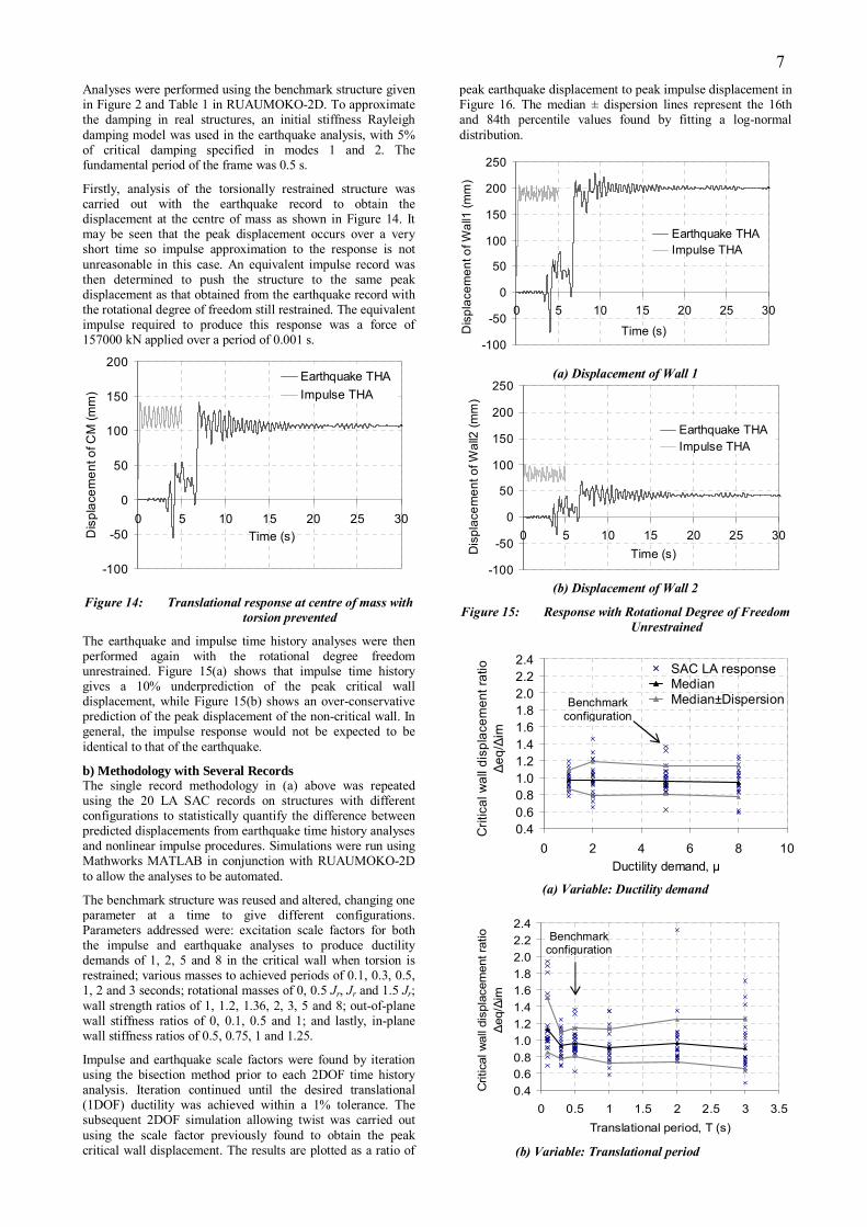
7
-100
-50
0
50
100
150
200
250
0 5 10 15 20 25 30Time (s)D
ispl
acem
ent o
f Wal
l2 (m
m)
Earthquake THAImpulse THA
0.40.60.81.01.21.41.61.82.02.22.4
0 0.5 1 1.5 2 2.5 3 3.5Translational period, T (s)
Crit
ical
wal
l dis
plac
emen
t rat
io∆
eq/∆
im
Benchmark configuration
-100
-50
0
50
100
150
200
250
0 5 10 15 20 25 30
Time (s)Dis
plac
emen
t of W
all1
(mm
)
Earthquake THAImpulse THA
0.40.60.81.01.21.41.61.82.02.22.4
0 2 4 6 8 10Ductility demand, µ
Crit
ical
wal
l dis
plac
emen
t rat
io∆e
q/∆i
m
SAC LA response Median Median±Dispersion Benchmark
configuration
-100
-50
0
50
100
150
200
0 5 10 15 20 25 30Time (s)D
ispl
acem
ent o
f CM
(mm
)
Earthquake THAImpulse THA
Analyses were performed using the benchmark structure given in Figure 2 and Table 1 in RUAUMOKO-2D. To approximate the damping in real structures, an initial stiffness Rayleigh damping model was used in the earthquake analysis, with 5% of critical damping specified in modes 1 and 2. The fundamental period of the frame was 0.5 s.
Firstly, analysis of the torsionally restrained structure was carried out with the earthquake record to obtain the displacement at the centre of mass as shown in Figure 14. It may be seen that the peak displacement occurs over a very short time so impulse approximation to the response is not unreasonable in this case. An equivalent impulse record was then determined to push the structure to the same peak displacement as that obtained from the earthquake record with the rotational degree of freedom still restrained. The equivalent impulse required to produce this response was a force of 157000 kN applied over a period of 0.001 s.
Figure 14: Translational response at centre of mass with torsion prevented
The earthquake and impulse time history analyses were then performed again with the rotational degree freedom unrestrained. Figure 15(a) shows that impulse time history gives a 10% underprediction of the peak critical wall displacement, while Figure 15(b) shows an over-conservative prediction of the peak displacement of the non-critical wall. In general, the impulse response would not be expected to be identical to that of the earthquake.
b) Methodology with Several Records The single record methodology in (a) above was repeated using the 20 LA SAC records on structures with different configurations to statistically quantify the difference between predicted displacements from earthquake time history analyses and nonlinear impulse procedures. Simulations were run using Mathworks MATLAB in conjunction with RUAUMOKO-2D to allow the analyses to be automated.
The benchmark structure was reused and altered, changing one parameter at a time to give different configurations. Parameters addressed were: excitation scale factors for both the impulse and earthquake analyses to produce ductility demands of 1, 2, 5 and 8 in the critical wall when torsion is restrained; various masses to achieved periods of 0.1, 0.3, 0.5, 1, 2 and 3 seconds; rotational masses of 0, 0.5 Jr, Jr and 1.5 Jr; wall strength ratios of 1, 1.2, 1.36, 2, 3, 5 and 8; out-of-plane wall stiffness ratios of 0, 0.1, 0.5 and 1; and lastly, in-plane wall stiffness ratios of 0.5, 0.75, 1 and 1.25.
Impulse and earthquake scale factors were found by iteration using the bisection method prior to each 2DOF time history analysis. Iteration continued until the desired translational (1DOF) ductility was achieved within a 1% tolerance. The subsequent 2DOF simulation allowing twist was carried out using the scale factor previously found to obtain the peak critical wall displacement. The results are plotted as a ratio of
peak earthquake displacement to peak impulse displacement in Figure 16. The median ± dispersion lines represent the 16th and 84th percentile values found by fitting a log-normal distribution.
(a) Displacement of Wall 1
(b) Displacement of Wall 2
Figure 15: Response with Rotational Degree of Freedom Unrestrained
(a) Variable: Ductility demand
(b) Variable: Translational period
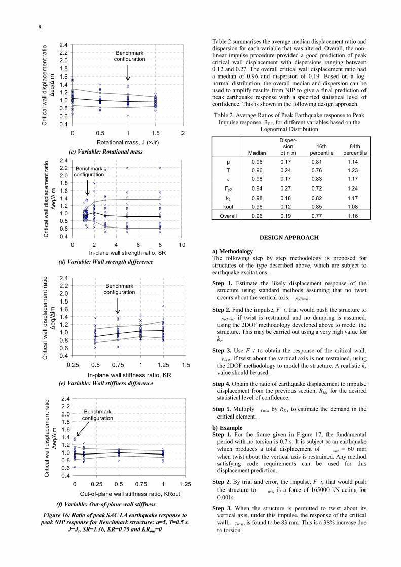
8
0.40.60.81.01.21.41.61.82.02.22.4
0.25 0.5 0.75 1 1.25 1.5
In-plane wall stiffness ratio, KR
Crit
ical
wal
l dis
plac
emen
t rat
io∆
eq/∆
im
Benchmark configuration
0.40.60.81.01.21.41.61.82.02.22.4
0 0.25 0.5 0.75 1 1.25
Out-of-plane wall stiffness ratio, KRout
Crit
ical
wal
l dis
plac
emen
t rat
io∆e
q/∆
im
Benchmark configuration
0.40.60.81.01.21.41.61.82.02.22.4
0 2 4 6 8 10In-plane wall strength ratio, SR
Crit
ical
wal
l dis
plac
emen
t rat
io∆
eq/∆
im
Benchmark configuration
0.40.60.81.01.21.41.61.82.02.22.4
0 0.5 1 1.5 2Rotational mass, J (×Jr)
Crit
ical
wal
l dis
plac
emen
t rat
io∆
eq/∆
imBenchmark
configuration
(c) Variable: Rotational mass
(d) Variable: Wall strength difference
(e) Variable: Wall stiffness difference
(f) Variable: Out-of-plane wall stiffness
Figure 16: Ratio of peak SAC LA earthquake response to peak NIP response for Benchmark structure: µ=5, T=0.5 s,
J=Jr, SR=1.36, KR=0.75 and KRout=0
Table 2 summarises the average median displacement ratio and dispersion for each variable that was altered. Overall, the non-linear impulse procedure provided a good prediction of peak critical wall displacement with dispersions ranging between 0.12 and 0.27. The overall critical wall displacement ratio had a median of 0.96 and dispersion of 0.19. Based on a log-normal distribution, the overall median and dispersion can be used to amplify results from NIP to give a final prediction of peak earthquake response with a specified statistical level of confidence. This is shown in the following design approach.
Table 2. Average Ratios of Peak Earthquake response to Peak Impulse response, RE|I, for different variables based on the
Lognormal Distribution
Median
Disper- sion σ(ln x)
16th percentile
84th percentile
µ 0.96 0.17 0.81 1.14 T 0.96 0.24 0.76 1.23 J 0.98 0.17 0.83 1.17
Fy2 0.94 0.27 0.72 1.24
k2 0.98 0.18 0.82 1.17 kout 0.96 0.12 0.85 1.08
Overall 0.96 0.19 0.77 1.16
DESIGN APPROACH a) Methodology The following step by step methodology is proposed for structures of the type described above, which are subject to earthquake excitations.
Step 1. Estimate the likely displacement response of the structure using standard methods assuming that no twist occurs about the vertical axis, NoTwist.
Step 2. Find the impulse, F t, that would push the structure to NoTwist if twist is restrained and no damping is assumed, using the 2DOF methodology developed above to model the structure. This may be carried out using a very high value for kr.
Step 3. Use F t to obtain the response of the critical wall, Twist, if twist about the vertical axis is not restrained, using the 2DOF methodology to model the structure. A realistic kr value should be used.
Step 4. Obtain the ratio of earthquake displacement to impulse displacement from the previous section, RE|I for the desired statistical level of confidence.
Step 5. Multiply Twist by RE|I to estimate the demand in the critical element.
b) Example Step 1. For the frame given in Figure 17, the fundamental
period with no torsion is 0.7 s. It is subject to an earthquake which produces a total displacement of wist = 60 mm when twist about the vertical axis is restrained. Any method satisfying code requirements can be used for this displacement prediction.
Step 2. By trial and error, the impulse, F t, that would push the structure to wist is a force of 165000 kN acting for 0.001s.
Step 3. When the structure is permitted to twist about its vertical axis, under this impulse, the response of the critical wall, Twist, is found to be 83 mm. This is a 38% increase due to torsion.
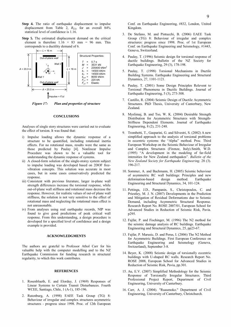
9
A = 20.0 m
A = 20.0 m
L = 16 m
L = 16 m x
y
Wall 1
Wall 2
M J
Out-of-plane wall
Out-of-plane wall
Impulse = Fi∆t
Structural Properties:
T = 0.7 s M = 3531 kN J = 235400 kNm2 k1 = 14500 kN/m k2 = 14500 kN/m kout = 8000 kN/m Fy1 = 220 kN Fy2 = Elastic
Step 4. The ratio of earthquake displacement to impulse displacement from Table 2, RE|I, for an overall 84% statistical level of confidence is 1.16.
Step 5. The estimated displacement demand on the critical element is therefore 1.16 × 83 mm = 96 mm. This corresponds to a ductility demand of 6.
Figure 17: Plan and properties of structure
CONCLUSIONS
Analyses of single story structures were carried out to evaluate the effect of torsion. It was found that:
i) Impulse loading allows the dynamic response of a structure to be quantified, including rotational inertia effects. For no rotational mass, results were the same as those predicted by Paulay [4]. Nonlinear Impulse Procedure was shown to be a valuable tool for understanding the dynamic response of systems.
ii) A closed-form solution of the single-storey system subject to impulse loading was developed based on 2DOF free-vibration concepts. This solution was accurate in most cases, but in some cases conservatively predicted the response.
iii) Consistent with previous literature, larger in-plane wall strength differences increase the torsional response, while out-of-plane wall stiffness and rotational mass decrease the response. However, for realistic values of out-of plane wall stiffness, the solution is not very sensitive to the effect of rotational mass and neglecting the rotational mass effect is not unreasonable.
iv) From analyses using real earthquake records, NIP was found to give good predictions of peak critical wall response. From this understanding, a design procedure is developed for a specified level of confidence and a design example is provided.
ACKNOWLEDGMENTS
The authors are grateful to Professor Athol Carr for his valuable help with the computer modelling and to the NZ Earthquake Commission for funding research in structural regularity, to which this work contributes.
REFERENCES
1. Rosenblueth, E. and Elorduy, J. (1969) Responses of Linear Systems to Certain Transit Disturbances. Fourth WCEE, Santiago, Chile, 1 (A-1), 185-196.
2. Rutenburg, A. (1998) EAEE Task Group (TG) 8: Behaviour of irregular and complex structures asymmetric structures - progress since 1998. Proc. of 12th European
Conf. on Earthquake Engineering, #832, London, United Kingdom.
3. De Stefano, M. and Pintucchi, B. (2006) EAEE Task Group (TG) 8: Behaviour of irregular and complex structures: progress since 1998. Proc. of 1st European Conf. on Earthquake Engineering and Seismology, #1443, Geneva, Switzerland.
4. Paulay, T. (1996) Seismic design for torsional response of ductile buildings. Bulletin of the NZ Society for Earthquake Engineering, 29 (3), 178-198.
5. Paulay, T. (1998) Torsional Mechanisms in Ductile Building Systems. Earthquake Engineering and Structural Dynamics, 27, 1101-1121.
6. Paulay, T. (2001) Some Design Principles Relevent to Torsional Phenomena in Ductile Buildings. Journal of Earthquake Engineering, 5 (3), 273-308.
7. Castillo, R. (2004) Seismic Design of Ductile Asymmetric Structures. PhD Thesis, University of Canterbury, New Zealand.
8. Myslimaj, B. and Tso, W. K. (2004) Desirable Strength Distribution for Asymmetric Structures with Strength-Stiffness Dependent Elements. Journal of Earthquake Engineering, 8 (2), 231-248.
9. Trombetti, T., Gasparini, G. and Silvestri, S. (2002) A new simplified approach to the analysis of torsional problems in eccentric systems: the “Alpha” method. Proc. Third European Workshop on the Seismic Behaviour of Irregular and Complex Structures (Firenze, Italy).Smith, W.D. (1995) “A development in the modeling of far-field intensities for New Zealand earthquakes”. Bulletin of the New Zealand Society for Earthquake Engineering. 28 (3). 196-217.
10. Sommer, A. and Bachmann, H. (2005) Seismic behaviour of asymmetric RC wall buildings: Principles and new deformation-based design method. Earthquake Engineering and Structural Dynamics, 34, 101-124.
11. Pettinga, J.D., Pampanin, S., Christopoulos, C. and Priestley, M. J. N. (2007) Developments in the Prediction and Mitigation of Residual Deformations due to Seismic Demand, including Asymmetric Structural Response. Research Report No. ROSE 2007/01, European School for Advanced Studies in Reduction of Seismic Risk, Pavia. p295.
12. Fajfar, P. and Fischinger, M. (1996) The N2 method for the seismic damage analysis of RC buildings. Earthquake Engineering and Structural Dynamics, 25, pp23-67.
13. Fajfar, P. Marusic, D. and Perus, I. (2006) The N2 Method for Asymmetric Buildings. First European Conference on Earthquake Engineering and Seismology (Geneva, Switzerland), September 3-8.
14. Beyer, K. (2008) Seismic design of torsionally eccentric buildings with U-shaped RC walls. Research Report No. ROSE 2008, European School for Advanced Studies in Reduction of Seismic Risk, Pavia, pp.301.
15. Au, E.V. (2007) Simplified Methodology for the Seismic Response of Torsionally Irregular Structures. Third Professional Project Report, Department of Civil Engineering, University of Canterbury.
16. Carr, A. J. (2004). "Ruaumoko." Department of Civil Engineering, University of Canterbury, Christchurch.
Structural Properties:
T = 0.7 s M = 3531 kN J = 235400 kNm2 k1 = 14500 kN/m k2 = 14500 kN/m kout = 8000 kN/m Fy1 = 220 kN Fy2 = Elastic

CHAPTER 6. DESIGN FOR TORSIONAL IRREGULARITY

1
CHAPTER 6. DESIGN FOR TORSIONAL IRREGULARITY In Chapter 5 it was shown that rotational mass tends to decrease the response of structures, but that this decrease is small for systems in with out-of-plane walls. Priestley et al. (2007) state that previous studies on torsional irregularity have found the following:
- for torsionally unrestrained (TU) systems (Priestley et al. p331) o the rotational mass effect is considerable o for structures with normal rotational mass designed considering no
strength eccentricity from the centre of mass, the displacements will not be greater than those estimated for zero strength eccentricity irrespective of the actual strength eccentricity
- for torsionally restrained (TR) systems (Priestley et al. p336)
o the displacement of the centre of mass is moves to the same displacement irrespective of whether or not torsion occurs
o for typical structures the response is insensitive to the amount of rotational mass, however increase of strength of any element in the system does not tend to increase the demand on any critical element
o by keeping the strength and stiffness eccentricity low (i.e. displacement between the centre of mass and/or centre of stiffness and strength), significant torsion can be largely avoided
o the torsional component of peak displacement increased with ductility o earthquake shaking in a skew direction, rather than along the building
principal axes, increased the displacements by less than 10%. o for the cases considered, when the transverse wall stiffness changed by
a factor of 2, and when some yielding occurred in the transverse walls, the demands on the in-plane walls did not change significantly.
Priestley has suggested the following approach for torsionally restrained and unrestrained systems (p337). The maximum displacements of a building plan are approximated by the translation of the centre of mass plus the displacements found by a nominal rotation through the centre of mass, N, given in Equation 1, where eR is the elastic stiffness eccentricity (measured between the centre of mass and the elastic centroid), Vdes is the design storey shear, and JR, is the ductile rotational stiffness given by Equation 2. Here kz is the stiffness in the z (loading) direction and kx is the stiffness in the x (transverse) direction, eRX and eRZ are the eccentricities in the X and Z directions respectively, and sys is the system ductility.
N = Vdes . eR (1) JR,
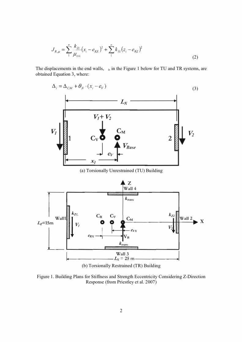
2
(2) The displacements in the end walls, i, in the Figure 1 below for TU and TR systems, are obtained Equation 3, where:
(3)
(a) Torsionally Unrestrained (TU) Building
(b) Torsionally Restrained (TR) Building
Figure 1. Building Plans for Stiffness and Strength Eccentricity Considering Z-Direction
Response (from Priestley et al. 2007)

3
Priestley et al (2007) claim that the approach outlined above has been checked against results of Castillo et al. and Beyer, “and found to give generally good agreement for both TU and TR systems”. An example for application is provided for a 6 storey structure. Relationship between i and JR, Based on the methodology of Priestley et al., a relationship between i and JR, may be obtained by rearranging the equations above. Here, the peak displacement of a wall, i, is assumed to be limited to a ratio, , of the displacement of the centre of mass, CM (which is assumed to be the same as the displacement of the structure if no translation occurs). For example, for an increase in displacement to 10% relative to the no-translation case, = 1.10.
i = 1 + N xi (4) CM CM
( -1) Vdes . eR xi (5)
JR, CM
JR, Vdes . eR xi (6) ( -1) CM Here it may be seen that to limit the torsional component of translation to smaller values (i.e. smaller ), higher values of ductile rotational stiffness JR, are required. For the case that = 1.1, the required value of JR, is:
JR, Vdes . eR xi (7) CM Note: The torsional response in the approach described above is dependent on the ductile rotational stiffness JR, . The equations indicate that doubling JR, implies halving the percentage increase in response. Therefore, a doubling of JR, would change from 1.1 to 1.2 only. It does not double . This is consistent with the findings of torsionally restrained systems by Priestley et al. (2007) in which the demands on the in-plane walls did not change significantly with a major change of transverse wall stiffness. Priestley M.J.N., Calvi G.M., Kowalsky M.J., “Displacement-Based Seismic Design of Structures”, IUSS Press, 2007. ISBN: 88-6198-000-6.

4
Design Example For a rectangular symmetric building with external walls of the same sise which resist seismic load eR = eV since the centres of the stiffness and strength are in the centre of the structure. (a) Resistance provided by walls a) Case 1: = 1 => JR, = kr2 = 4 kr2 b) Case 2: = 4 => JR, = kr2 = 2 kr2 + 2 kr2/4 = 2.5 kr2 (b) Demand
JR, Vdes . eR xi CM = des ( -1) CM
Vdes . eR xi Vdes = 2k ( -1) des des
2k eR xi eR = r , xi = r + r ( -1) 2k r2(1 + ( -1)
r r
eR
r = b/2
r
k
k Fy
k Fy
CM CS

5
Comparison (a) = 1
4 kr2 2k r2 (1 +
( -1) so (1 + If = 0.2 (i.e. eacc = 0.1b) then If = 0.1 (i.e. eacc = 0.05b) then
Therefore, for small values of eacc, the fraction of b is close to the fraction change in response.
Comparison (b) = 4
2.5 kr2 2k r2 (1 +
( -1) so (1 + If = 0.2 (i.e. eacc = 0.1b) then Based on the above comparison it may be seen that the response is expected to decrease from 1.12 to 1.048 as a result of the increased ductility. This is because a lower total force gets into the system. The out-of-plane walls resist torsion due to this lower force more than they do due to a higher force.

6
Possible Alternative Approach The approach by Priestley et al. (2007) described above was developed within a Displacement Based Design (DBD) context, and was applied above to structures irrespective of the design approach. While many of the equations are given in Beyer (2007) the full derivation of those equations is not provided in that report. An alternative approach is developed below. It is similar to that described above, but it is believed to be simpler, transparent, and a full derivation of the approach is given. AIM: The aim is to limit the displacement resulting from torsion to no more
than times the displacement at the centre of mass by providing sufficient torsional restraint. (This is similar to that described above)
ASSUMPTIONS: 1) The centre of mass of the structure moves to the same
displacement irrespective of the torsional deformation 2) The structure has torsional restraint 3) Effects of torsional mass can be ignored without significant error
4) Earthquake shaking in a skew direction, rather than along the building principal axes, does not significantly increase the displacements
APPROACH: The out-of-plane walls provide a rotational stiffness, k , with units of Nm. This rotational stiffness is computed as: k M/ If there are two walls providing restraint in the transverse (z) direction, as shown in Figure 2, then k is computed about the centre of stiffness (CS) of these walls as: k kz z dxb kz z dxt / kz dxb
2 kz dxt 2 /
∑kz dxi
2 The rotation demand, M, is given below where V is the actual shear force acting in the storey below the level considered, and ez is the eccentricity in the direction perpendicular to the direction of shaking. For an elastically loaded structure, the eccentricity is the distance between the centre of stiffness and the centre of mass. For a structure in which significant yielding is expected, the eccentricity is the distance between the centre of stiffness and the centre of mass. Conservatively for both cases it may be taken as the maximum of these two distances. That is ez = max{ezv, ezs}.

7
M = Vez Under this moment it is required that the maximum displacement at an extreme element be no more than cm, where is a value greater than unity, and cm is the computed displacement of the storey assuming no twist using standard methods. Here zmax is the distance in the z direction to the wall with the critical (and possibly maximum) displacement. To ensure this; < ( x,max - cm) /z,max = ( ) cm/zmax But = M/k = Vez /k Therefore: k Vez zmax ( ) cm Since V = ∑kxi cm/ act, where act is the actual system ductility as defined in the appropriate materials code, the above equation may be written as: Therefore: k ez.zmax.∑kxi ( ) act For a square building in which the centre of mass is 0.10b from the centre of the building, in which a displacement increase of no more than 10% is desired, and the design ductility was 5 but the actual ductility was 2.5, AND all transverse walls have the same stiffness, and all longitudinal walls have the same stiffness, then and
b
z1
dx2
kz2
kx1 Fyx1
CM
dx1
kz1
z
x
CS CV
kx2 Fyx2
ezs
ezv
8
k ∑kz dxi
2 ez.zmax.∑kxi
( ) kz x 2 x dx/2)2
ez.zmax.2kx kz d2/2 8 x 0.10d. x 0.4d.2kx kz 0.64 kx implying that having the same amount of wall stiffness in both directions is sufficient for this case. The approach outlined above is conceptually clean. It is derived using the centre of mass as the reference point. It is slightly more conservative than that of Priestley et al. (2007), because the effect of in-plane walls on the rotational stiffness is ignored. It has not been calibrated against test results so would require further verification before it is used.


CHAPTER 7. DIAPHRAGM FLEXIBILITY
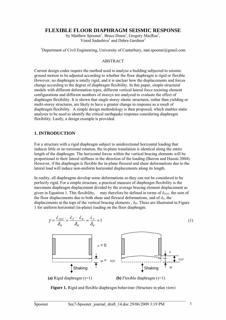
Spooner Sec7-Spooner_journal_draft_14.doc 29/06/2009 3:19 PM 1
FLEXIBLE FLOOR DIAPHRAGM SEISMIC RESPONSE by Matthew Spooner1, Bruce Deam1, Gregory MacRae1,
Vinod Sadashiva1 and Debra Gardiner1
1Department of Civil Engineering, University of Canterbury, [email protected]
ABSTRACT Current design codes require the method used to analyse a building subjected to seismic ground motion to be adjusted according to whether the floor diaphragm is rigid or flexible. However, no diaphragm is totally rigid, and it is unclear how the displacements and forces change according to the degree of diaphragm flexibility. In this paper, simple structural models with different deformation types, different vertical lateral force resisting element configurations and different numbers of storeys are analyzed to evaluate the effect of diaphragm flexibility. It is shown that single storey elastic structures, rather than yielding or multi-storey structures, are likely to have a greater change in response as a result of diaphragm flexibility. A simple design methodology is then proposed, which enables static analyses to be used to identify the critical earthquake response considering diaphragm flexibility. Lastly, a design example is provided.
1. INTRODUCTION For a structure with a rigid diaphragm subject to unidirectional horizontal loading that induces little or no torsional rotation, the in-plane translation is identical along the entire length of the diaphragm. The horizontal forces within the vertical bracing elements will be proportional to their lateral stiffness in the direction of the loading (Barron and Hueste 2004). However, if the diaphragm is flexible the in-plane flexural and shear deformations due to the lateral load will induce non-uniform horizontal displacements along its length. In reality, all diaphragms develop some deformations so they can not be considered to be perfectly rigid. For a simple structure, a practical measure of diaphragm flexibility is the maximum diaphragm displacement divided by the average bracing element displacement as given in Equation 1. This flexibility, may therefore be defined in terms of δTOT, the sum of the floor displacements due to both shear and flexural deformations, and of δF, the displacements at the tops of the vertical bracing elements , δW. These are illustrated in Figure 1 for uniform horizontal (in-plane) loading on the floor diaphragm.
1+=+==W
F
W
WF
W
TOT
δδ
δδδ
δδγ (1)
(a) Rigid diaphragm (γ=1) (b) Flexible diaphragm (γ>1)
Figure 1. Rigid and flexible diaphragm behaviour (Structure in plan view)
W = TOT
F = 0
Shaking W Shaking
F
TOT
Spooner Sec7-Spooner_journal_draft_14.doc 29/06/2009 3:19 PM 2
The effect of flexibility could be considered by explicitly modelling the diaphragm response using 3-D dynamic time history analyses to verify a design, but the additional complexity probably ensures that this is seldom used in the design office. For the more common types of analysis method, international seismic codes (e.g. NZS1170.5, 2004) generally require floor diaphragms to be treated as being either perfectly “rigid”, in which case the demands on lateral force resisting systems are related to those of the adjacent systems; or as completely “flexible” so the lateral forces can be distributed between bracing elements on a tributary area basis. In the New Zealand Structural Design Actions Standard, NZS1170.5, Clause 6.1.4.1 specifies that “[w]here diaphragms are not rigid compared to the vertical elements of the lateral [load]-resisting system, the model should include representation of the diaphragm’s flexibility”. Appendix A defines a “flexible diaphragm” as one “that is sufficiently flexible that the maximum lateral deformation of the diaphragm alone is more than twice the average inter-storey deflection at that level”. Since the value considers the total deflection, which is equal to the diaphragm deformation plus the storey deformation in the numerator, the code requirement corresponds to > 3 for a flexible diaphragm with < 3 for a rigid diaphragm. BSSC FEMA250 (2003) has identical requirements (Clause 4.3.2.1). The boundary value at = 3 is based on engineering judgement rather than quantitative analyses (SEAOC, 1999), and there are no requirements to consider displacements or forces resulting from diaphragm flexibility. Furthermore, if seismic displacements generated in a structure with a flexible diaphragm are greater than those where a rigid diaphragm is assumed, or if the forces or deformations developed in some elements are greater due to diaphragm flexibility, then the rigid diaphragm design assumption would be non-conservative. This paper aims to address the issues outlined above by answering the following questions for simple structures which are not subject to significant torsion:
(1) When a diaphragm is flexible, how does it affect the displacement demands and the design actions (i.e. internal shear forces and moments) for the diaphragm and bracing elements?
(2) Do the relative portions of flexural and shear deformations within a flexible diaphragm influence the displacement demands or design actions?
(3) How does yielding of the bracing elements affect the demands or actions? (4) How does structural complexity affect the variation of demands? (5) How do the demands change for multi-storey structures? (6) Can simple rational design recommendations be developed?
To answer these questions, previous studies of diaphragm flexibility are briefly reviewed and structural models are used to evaluate the effects of in-plane diaphragm flexibilities when subjected to a suite of ground motion records. Simple single storey elastic models, models with yielding bracing elements, models with different bracing wall arrangements, and multi-storey structural models are all considered.
2. PREVIOUS RESEARCH ON DIAPHRAGM FLEXIBILITY Fleischman and Farrow (2001) studied the dynamic behaviour of structures with perimeter bracing systems and flexible diaphragms using both modal and inelastic dynamic time-history analyses. They found that diaphragm flexibility can increase force demands in shear wall structures which have very short periods, and that for multi-storey structures, inelasticity causes the major deformation demands to occur within the lower levels.

Spooner Sec7-Spooner_journal_draft_14.doc 29/06/2009 3:19 PM 3
Paquette, Bruneau and Brzev (2004) pseudo-dynamically tested a full-scale masonry building containing a wood diaphragm. The in-plane deflected shape of the diaphragm was symmetric and similar to that predicted using a pinned-pinned beam model. Although the diaphragm was not tested to its ultimate capacity, it was shown that deflections were primarily due to flexural deformations, rather than the commonly assumed shear deformations. Lee, Ashheim and Kuchma (2006) also reported significant flexural deformations within a flexible diaphragm. Fleischman and Farrow (2003) showed that the relatively flexible connections between the precast segments within long-span precast concrete floor diaphragms made them inherently more flexible than monolithic floor systems. Their design recommendations suggested using a flexibility index to define the diaphragm design strength and ductility capacity. Lee, Kuchma and Ashheim (2006) described a method of estimating interstorey drifts for preliminary design. Their method is based on a principle components analysis (PCA), which determines the dominant modes in the structure and assesses the contribution each mode makes to the overall response. They found that flexible diaphragm structures had significant modal correlation due to their closely spaced deformation modes. Their time-history analyses showed that the drift demands tended to be greatest at the lowest levels of their structures. Sullivan (2006) analysed 8, 16 and 20 storey structures with floor plan aspect ratios of 10:3. The slab flexural stiffness was reduced to 25% of the gross section stiffness to accommodate concrete cracking. The increased diaphragm flexibility was found to have little effect on interstorey drifts, floor moments and floor shear. Gulay et al. (2006) reported that the responses of structures with wall bracing elements were more significantly affected than those with either frames, or combinations of frames and walls. The differences were attributed to the high relative wall stiffness.
3. MODELLING STRUCTURES WITH FLEXIBLE DIAPHRAGMS
3.1 Single Storey Model The most elementary model that can be employed to investigate floor diaphragm flexibility is the single-storey structure shown in Figure 2(a) with two parallel bracing elements and a floor diaphragm at each. While the bracing elements in this figure are illustrated as walls, they could be any combination of frame and wall components.
(a) Schematic of single storey structure (b) Plan view of the structural model
Figure 2. Single-storey wall and floor diaphragm structure used to investigate the effects of floor diaphragm flexibility
Spooner Sec7-Spooner_journal_draft_14.doc 29/06/2009 3:19 PM 4
For this study, the Figure 2(a) structure was modelled using springs to represent the bracing elements and a simply-supported flexural beam used to represent the floor diaphragm as shown in the Figure 2(b) plan view. In this model, m is the total beam mass, E and G are the elastic and shear modulii respectively, Ix is the moment of inertia, As is the shear area, and the lateral wall stiffness is kW.
3.2 Analysis Methodology The fundamental period of a structure with a rigid diaphragm, TRIGID, is related to the diaphragm mass, m, and the bracing wall stiffness, kW. This definition assumes that the mass of the walls is insignificant compared to the mass of the diaphragm.
WRIGID k
mT π2= (2)
The fundamental period increase, TINCR, for a structure with a flexible diaphragm was made non-dimensional by dividing its elastic fundamental period by the fundamental period of an otherwise identical structure with a rigid diaphragm, TRIGID. The diaphragm displacements, bracing wall shear forces and diaphragm bending moments provide indicative demand properties for the structure. These characteristics were considered best represented by the non-dimensional dynamic displacement ratio, MAX,RATIO, the wall shear force ratio, VRATIO, and the diaphragm bending moment ratio, MRATIO. These are defined in Equations 3 to 5, where δ is displacement, V is shear force, M is bending moment. The FLEX subscripts indicate a flexible diaphragm and RIGID a rigid diaphragm.
RIGIDTOT
FLEXTOTRATIOMAX
,
,, δ
δδ = (3)
RIGID
FLEXRATIO V
VV = (4)
RIGID
FLEXRATIO M
MM = (5)
Spooner (2008) showed that these dimensionless demand parameters were independent of the diaphragm span, aspect ratio and construction material. This means that general recommendations can be developed. The following steps were used to calculate these non-dimensional demand parameters for a suite of ground motion records using the RUAUMOKO-3D non-linear integrated time-history analysis package (Carr, 2007): Step 1. Design a suite of structures by selecting an appropriate range of rigid
fundamental periods, TRIGID, and estimate the wall stiffness, kW, associated with each period for a diaphragm mass, m. The wall stiffness is calculated using the rearranged form of Equation 2:
RIGIDW T
mk24π= (6)

Spooner Sec7-Spooner_journal_draft_14.doc 29/06/2009 3:19 PM 5
Step 2. Select an appropriate range of diaphragm flexibility γ, and use a static analysis to calculate the diaphragm stiffness, kF, for each γ. Equation 1 is rearranged to calculate the diaphragm stiffness, kF, as:
1// +=γ
W
F
kFkF
(7)
1−γ= W
Fkk (8)
Step 4. Assuming a realistic value for the modulus of elasticity, E, calculate the
second moment of area, Ix using statics. For a uniformly distributed load applied to a simply-supported beam, the midspan flexural displacement, B(L/2), is calculated as:
XB EI
wLL384
5)2/(4
=δ (9)
Step 5. Analyse each structure’s response to each of the 20 ground motion records
within the SAC suite that is scaled to provide a probability of 10% in 50 years for Los Angeles (SAC Steel, 2002).
Then, for every ground motion record and for every combination of TRIGID,
and γ:
Step 5 a. Calculate TFLEX, the peak displacement, δTOT, the maximum diaphragm displacement, δF, the corresponding wall displacement, δW, the maximum wall shear force, VFLEX, and the diaphragm bending moment, MFLEX.
Step5 b. Calculate the dimensionless fundamental period increase, TINCR, wall shear force ratio, peak displacement increase, δMAX,RATIO, dynamic displacement ratio, δRATIO, fundamental natural period increase, VRATIO, and diaphragm bending moment ratio, MRATIO.
Step 6. Calculate the median value of each non-dimensional demand indicator calculated in step 5 for each of the 20 records and plot them separately, using γ as the independent variable.
This methodology was used for a number of structures with different values of γ, representing diaphragm flexibility, and rigid fundamental periods, implicitly representing wall stiffness. A diaphragm flexibility range of 1 ≤ ≤ 4 and discrete periods of TRIGID, = 0.1, 0.5, 1 and 2.0 s were considered to provide representative characteristics for many buildings. All of the analyses reported in the remainder of this paper were conducted using this methodology. Also, all of the analyses were conducted with the initial-stiffness proportional constant damping of 5% for all modes.
3.3 Diaphragm Models: While the bracing wall elements could be conveniently but realistically idealized as springs with no mass, there are several models that could be used for the diaphragm. The diaphragm would probably be best represented either using three-dimensional finite elements or using an assemblage of plane-stress membrane elements (for the floor) and either beams or struts (for the perimeter frames). Finite element analysis may best capture the real behaviour (Chopra 2000) but this introduces additional complexity, both in the work required to conduct and
Spooner Sec7-Spooner_journal_draft_14.doc 29/06/2009 3:19 PM 6
interpret the analysis and in accurately defining the connections between the diaphragm and its bracing walls. It was therefore decided to use less elaborate beam elements to model the diaphragm, which narrowed the choice to elements implementing either Euler/Bernoulli beam theory or Timoshenko beam theory. Euler/Bernoulli theory is adequate for long, thin beams with dominantly flexural deformations, whereas Timoshenko beam theory is more appropriate for short and deep beams where shear deformations are significant (Timoshenko 1922). A lumped mass model with eight beam elements was chosen to approximate the diaphragm and its distributed mass. While consistent mass models can provide better accuracy, they require greater computational effort and make displaced shape approximations that could bias the time-history analyses (Clough and Penzien, 1993). The diaphragm was therefore modelled using lumped masses and the minimum of eight beam elements required to obtain accurate shear and flexural forces (Lee, Kuchma and Ashheim, 2006; Spooner, 2008). The analysis methodology outlined in the previous section was used to compare the difference between diaphragm behaviour modelled using the Euler-Bernoulli and Timoshenko beam theories. Both were modelled using the Timoshenko beam element within RUAUMOKO, with the flexural (Euler-Bernoulli) diaphragm approximation modelled using a realistic elastic modulus (E) and a very large shear modulus (G) and a shear (Timoshenko) beam with a very large E and realistic G. The average period increases plotted in Figure 3(a) show little difference between the flexural and shear representations for a wide range of static displacement ratios and for three different natural periods, TRIGID = 0.1, 1.0 and 2.0 s. The period increases are independent of the natural period because they are calculated using an elastic eigenvalue analysis. The minor differences between the two beam theories were most likely due to a combination of using a finite number of segments to model the diaphragm and the small differences between the static deflections, calculated using uniformly distributed loads, and the dynamic deflections, which are expected to have a more sinusoidal distribution. The average peak displacement increases plotted in Figure 3(b) also show little difference between the shear and flexural beam models. There were minor differences in behaviour observed for the other characteristic parameters. At low levels of flexibility, particular for γ < 2, there was little practical difference in response. Shear deformations were therefore ignored and the remainder of the analyses reported in this paper only used the Euler-Bernoulli flexural beam model.

Spooner Sec7-Spooner_journal_draft_14.doc 29/06/2009 3:19 PM 7
0
10
20
30
40
50
60
70
80
90
1 1.5 2 2.5 3 3.5 4
Static Displacement Ratio, γ
Nat
ural
Per
iod
Incr
ease
, TIN
CR (%
)
Euler-Bernoulli
Timoshenko
(a) Increase in natural period
(b) Increase in peak displacement
Figure 3. Comparison of Timoshenko and Euler-Bernoulli median response for 20 SAC LA records
1
1.5
2
2.5
3
3.5
4
4.5
5
1 1.5 2 2.5 3 3.5 4
Static Displacement Ratio, γ
Peak
Dis
plac
emen
t Inc
reas
e, δ
MA
X,R
ATI
O
Euler-Bernoulli
Timoshenko
T = 0.1s
T = 1.0s
T = 2.0s
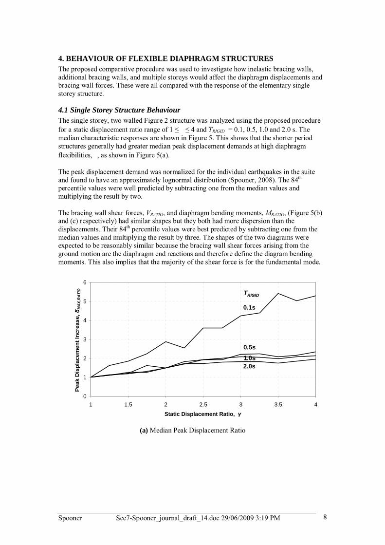
Spooner Sec7-Spooner_journal_draft_14.doc 29/06/2009 3:19 PM 8
4. BEHAVIOUR OF FLEXIBLE DIAPHRAGM STRUCTURES The proposed comparative procedure was used to investigate how inelastic bracing walls, additional bracing walls, and multiple storeys would affect the diaphragm displacements and bracing wall forces. These were all compared with the response of the elementary single storey structure.
4.1 Single Storey Structure Behaviour The single storey, two walled Figure 2 structure was analyzed using the proposed procedure for a static displacement ratio range of 1 ≤ ≤ 4 and TRIGID = 0.1, 0.5, 1.0 and 2.0 s. The median characteristic responses are shown in Figure 5. This shows that the shorter period structures generally had greater median peak displacement demands at high diaphragm flexibilities, , as shown in Figure 5(a). The peak displacement demand was normalized for the individual earthquakes in the suite and found to have an approximately lognormal distribution (Spooner, 2008). The 84th percentile values were well predicted by subtracting one from the median values and multiplying the result by two. The bracing wall shear forces, VRATIO, and diaphragm bending moments, MRATIO, (Figure 5(b) and (c) respectively) had similar shapes but they both had more dispersion than the displacements. Their 84th percentile values were best predicted by subtracting one from the median values and multiplying the result by three. The shapes of the two diagrams were expected to be reasonably similar because the bracing wall shear forces arising from the ground motion are the diaphragm end reactions and therefore define the diagram bending moments. This also implies that the majority of the shear force is for the fundamental mode.
0
1
2
3
4
5
6
1 1.5 2 2.5 3 3.5 4Static Displacement Ratio, γ
Peak
Dis
plac
emen
t Inc
reas
e, δ
MA
X,R
ATI
O TRIGID
0.1s
0.5s
1.0s2.0s
(a) Median Peak Displacement Ratio

Spooner Sec7-Spooner_journal_draft_14.doc 29/06/2009 3:19 PM 9
0
0.2
0.4
0.6
0.8
1
1.2
1.4
1.6
1 1.5 2 2.5 3 3.5 4Static Displacement Ratio, γ
Peak
Wal
l She
ar F
orce
Incr
ease
, V R
ATI
O
TRIGID
0.1s
0.5s
1.0s
2.0s
(b) Median Wall Shear Force Ratio
0
0.2
0.4
0.6
0.8
1
1.2
1.4
1.6
1.8
1 1.5 2 2.5 3 3.5 4
Static Displacement Ratio, γ
Dia
phra
gm M
omen
t Inc
reas
e, M
RA
TIO TRIGID
0.1s
0.5s
1.0s2.0s
(c) Median Diaphragm Bending Moment Ratio
Figure 5. Effect of Diaphragm Flexibility on Median Structural Response
TRIGID = 0.1, 0.5, 1.0, 2.0s, SAC LA10in50 records The Figure 5 relationships between TRIGID and demand are related to the period increase arising from additional diaphragm flexibility, which are in turn defined by the acceleration spectrum. The median acceleration response spectrum for the ground motion records is shown in Figure 6(a). For structures with a period less than the T = 0.3 s peak, the increased diaphragm flexibility increases the acceleration and the peak force. For longer period structures, the peak acceleration and force tend to decrease. Similarly, the period increase tends to increase in peak displacement responses of the structures used in this study as shown in Figure 6(b). Quantitative examples of these differences will be shown later.

Spooner Sec7-Spooner_journal_draft_14.doc 29/06/2009 3:19 PM 10
0
0.01
0.02
0.03
0.04
0.05
0.06
0 0.5 1 1.5 2 2.5 3 3.5 4
Period (s)
Spec
tral
Dis
plac
emen
t (m
)
0.
0.
0.
0.
0.
0.
Spec
tral
Dis
plac
emen
t (m
)
(a) Spectral Acceleration
(b) Spectral Displacement
Figure 6. Median Response Spectra 5% damping, 20 SAC LA 10in50 Records (from Singh 2008)
0
0.2
0.4
0.6
0.8
1
1.2
1.4
0 0.5 1 1.5 2 2.5 3 3.5 4
Period (s)
Spec
tral
Acc
eler
atio
n (m
/s2 )
Spec
tral
Acc
eler
atio
n(g)

Spooner Sec7-Spooner_journal_draft_14.doc 29/06/2009 3:19 PM 11
4.2 Effect of Bracing Wall Inelasticity Most structures will be designed to sustain inelastic displacements in their bracing walls or frames. For TRIGID > 0.3 s, the diaphragm deformations are expected to be smaller than when the bracing walls remain elastic because the bracing wall forces and therefore the diaphragm moments and deformations will be smaller. This was investigated using the proposed procedure with the wall yield strength, Fy, reduced from the maximum elastic shear force, Felastic, by dividing it by the lateral force reduction factor, kµ:
µ
=k
FF elastic
y (10)
The building responses were reasonably similar for a range of values of kµ, so a representative reduction factor of kµ = 1.5 was adopted for the analyses described below. The bracing walls were modelled using an elasto-plastic hysteresis model. As expected, the peak displacement increase, δMAX,RATIO for the yielding walls was generally less than it was for elastic bracing walls as shown in Figure 7 for rigid diaphragm structures with periods of 0.5 s and 1.0 s.
0
1
2
3
4
5
6
1 1.5 2 2.5 3 3.5Static Displacement Ratio, γ
Peak
Dis
plac
emen
t Inc
reas
e, δ
MA
X,R
ATI
O
Elastic Walls
Yielding Walls
TRIGID
0.1s
1.0s
0.5s
Figure 7. Median Displacement Ratio Increase
TRIGID = 0.1s, 0.5s and 1.0s, kµ = 1.5, 20 SAC LA 10in50 records However, for short period structures, such as the structure with TRIGID = 0.1 s shown in Figure 7, the overall displacement demand increased with increased inelasticity. This is most likely because displacements for short period, inelastic structures with rigid diaphragms are typically greater than they are for their elastic counterparts. When diaphragm flexibility was included, the additional bracing wall deformations were sometimes greater than the corresponding reduction in diaphragm deformation and at other times they were smaller. The combined effects of diaphragm flexibility and bracing wall inelasticity are therefore concluded to generally produce lower demands than elastically responding structures. For this reason, only the more critical elastically responding models were used for further analyses.
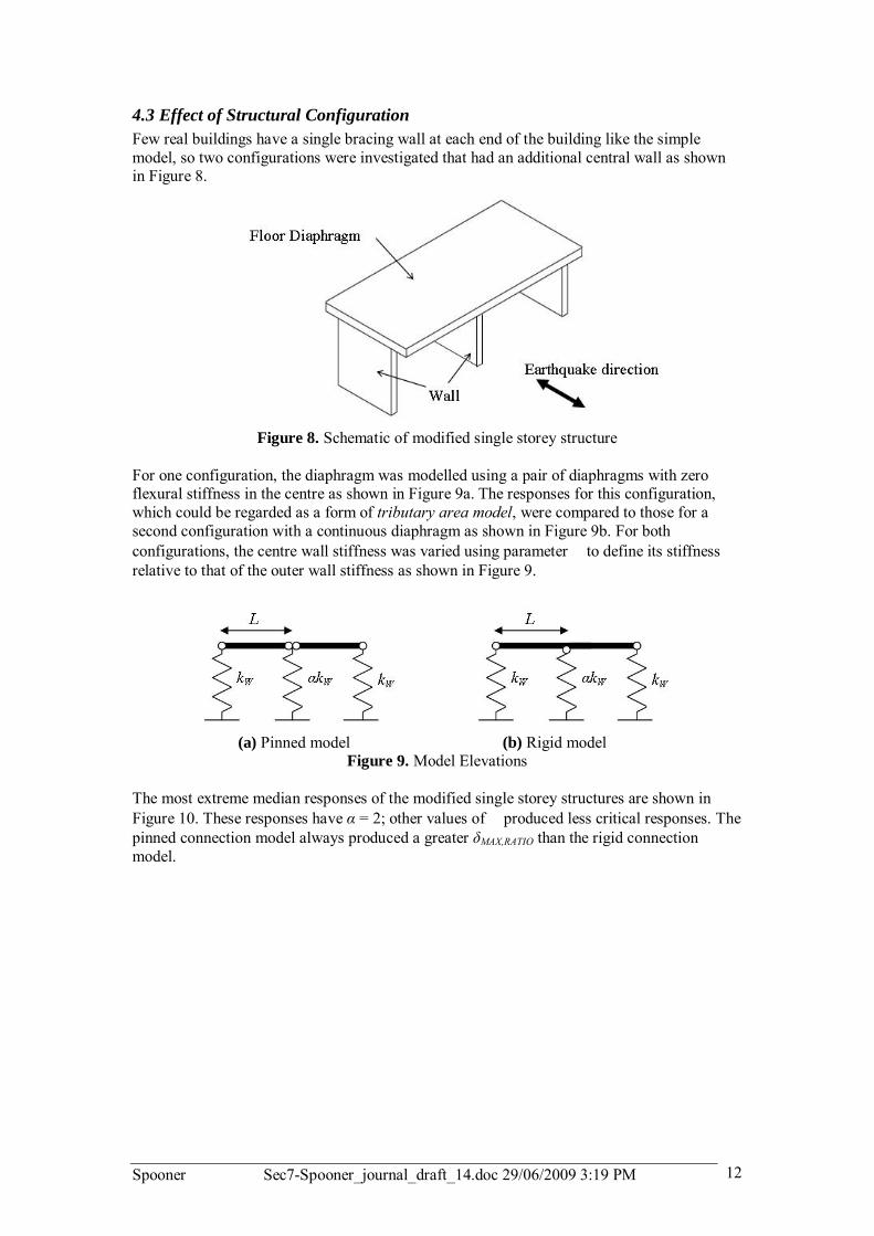
Spooner Sec7-Spooner_journal_draft_14.doc 29/06/2009 3:19 PM 12
4.3 Effect of Structural Configuration Few real buildings have a single bracing wall at each end of the building like the simple model, so two configurations were investigated that had an additional central wall as shown in Figure 8.
Figure 8. Schematic of modified single storey structure
For one configuration, the diaphragm was modelled using a pair of diaphragms with zero flexural stiffness in the centre as shown in Figure 9a. The responses for this configuration, which could be regarded as a form of tributary area model, were compared to those for a second configuration with a continuous diaphragm as shown in Figure 9b. For both configurations, the centre wall stiffness was varied using parameter to define its stiffness relative to that of the outer wall stiffness as shown in Figure 9.
(a) Pinned model (b) Rigid model
Figure 9. Model Elevations The most extreme median responses of the modified single storey structures are shown in Figure 10. These responses have α = 2; other values of produced less critical responses. The pinned connection model always produced a greater δMAX,RATIO than the rigid connection model.

Spooner Sec7-Spooner_journal_draft_14.doc 29/06/2009 3:19 PM 13
0.5
1
1.5
2
2.5
3
3.5
4
4.5
1 1.5 2 2.5 3
Static Displacement Ratio, γ
Peak
Dis
plac
emen
t Inc
reas
e, δ
MA
X,R
ATI
OPinned
Fixed
TRIGID
0.1s
0.5s1.0s
0.1s1.0s0.5s
Figure 10. Median Displacement Increase for Modified Configurations
TRIGID = 0.1s, 0.5s and 1.0s, = 2, 20 SAC LA 10in50 records The median displacement increases were all smaller than those for the simple structure (Figure 5b). As this occurred with both modified configurations, only the simple model was used for further analyses.
4.4 Effect of Number of Stories The elastic three storey structure shown in Figure 11 was used to evaluate the effect diaphragm flexibility had on multi-storey buildings. All six bracing wall segments had the same stiffness and the three floor diaphragms were identical.
Figure 11. Multistory Structure (Not to Scale)
This structure was analyzed using the proposed procedure with a static displacement ratio range of 1 ≤ ≤ 3. The median displacement increases of the three diaphragms and the wall force increases are shown in Figure 12 for TRIGID = 0.1 s. Similar behaviour was observed for other values of TRIGID. The maximum diaphragm displacement demand occurred in the lowest level (Figure 12a), which is consistent with observations by Lee et al. (2006) and Fleischman and Farrow (2001). The displacement increases for levels two and three were very similar. The shear force increase was greatest at the base of the structure as shown in Figure 12b.

Spooner Sec7-Spooner_journal_draft_14.doc 29/06/2009 3:19 PM 14
1
1.1
1.2
1.3
1.4
1.5
1.6
1.7
1 1.5 2 2.5 3
Static Displacement Ratio, γ
Peak
Dis
plac
emen
t Inc
reas
e, δ
MA
X,R
ATI
O
Level 1
23
(a) Peak displacement at each level
0.8
0.85
0.9
0.95
1
1.05
1.1
1.15
1.2
1.25
1 1.5 2 2.5 3
Static Displacement Ratio, γ
Peak
Wal
l She
ar F
orce
Incr
ease
, VR
ATI
O
Level 123
(b) Wall Shear Force at each level
Figure 12. Median Response of 3-Storey Structure
TRIGID = 0.1s, 20 SAC LA 10in50 records The displacement increases were significantly less than those for the single storey structure. This is illustrated in Figure 13, where the Figure 5(b) maximum response for the single storey structure (also with TRIGID = 0.1 s) is plotted with a broken line. The bracing wall forces at the base were also smaller.

Spooner Sec7-Spooner_journal_draft_14.doc 29/06/2009 3:19 PM 15
1
1.5
2
2.5
3
3.5
4
4.5
1 1.5 2 2.5 3
Static Displacement Ratio, γ
Peak
Dis
plac
emen
t Inc
reas
e, δ
MA
X,R
ATI
OMultistorey
Single Storey
Level 123
Figure 13. Median Displacement Increase for Lower Level of 3-Storey Structure and Single
Storey Structure, TRIGID = 0.1s, 20 SAC LA 10in50 records
5. DEVELOPMENT OF MODELS TO PREDICT RESPONSE It was expected that the floor diaphragm within a single storey structure could be reasonably well modelled as a simply supported beam with uniformly distributed mass and stiffness. If this in turn was able to be modelled as a single degree of freedom (SDOF) component, with an effective stiffness and an effective mass, a simple lumped mass model could be used to approximate the response of a single storey structure with a flexible diaphragm and bracing walls.
5.1 Lumped Mass Model for a Beam with Distributed Mass Singh (2008) developed a lumped mass approximation for a simply supported beam with uniformly distributed mass and stiffness using the fundamental mode shape φ (x) at position x along a simply-supported beam of length L (Clough and Penzien, 1993):
)sin()(Lxx πφ = (11)
The effective stiffness, EK, generalized mass, GM, and generalised excitation, GE, for the first mode for the beam with uniform mass per unit length, ρ , and uniform stiffness, EI, are (Clough and Penzien, 1993):
EIL
dxLx
LEIdxxEIEK
L
x
L
x 3
4
0
22
22
0 2)(sin)]("[ πππφ === ∫∫ ==
(12)
2)(sin)]([
0
2
0
2 LdxLxdxxGM
L
x
L
x
ρπρφρ === ∫∫ == (13)
πρπρρφ Ldx
LxdxxGE
L
x
L
x
2)sin()(00
=== ∫∫ == (14)

Spooner Sec7-Spooner_journal_draft_14.doc 29/06/2009 3:19 PM 16
These were used to create a single degree of freedom (SDOF) lumped mass and stiffness approximation of the first mode for the beam (Singh 2008) with an effective mass, EM, and stiffness, EK, defined above as shown in Figure 14. The effective mass is only a portion of the total beam mass and the displacement of the effective mass is smaller than the mid-span displacement of the distributed mass beam that it approximates.
Figure 14. Equivalent SDOF system for a beam with distributed mass
The participation factor, Γ, required to calculate the effective mass is:
πρπρ 422 ===Γ
LL
GMGE
(15)
The effective mass, EM, is therefore:
22
2 824πρ=
πρ
π=⋅Γ=⋅Γ== LLGEGM
GMGEEM (16)
For convenience in defining the structure in the next section, this is defined as a portion, , of the total diaphragm mass, mSDOF = L, giving:
SDOFmEM β= (17)
22
818π
=ρπ
ρ==βL
LmEM
SDOF
(18)
Similarly, if the effective stiffness is defined as a portion of the stiffness SDOFk for a beam with a point load applied at mid-span, the portion, , is calculated from the mid-span deflection, ∆, and point load, P, as:
SDOFkEK α= (19)
3
48LEIPkSDOF =
∆= (20)
96482
43
3
4 ππα ===EI
LLEI
kEK
SDOF
(21)
5.2 Two Degree-of-Freedom Approximation The SDOF lumped mass model defined has rigid supports and needed modifying to include wall flexibility. A two degree-of-freedom (2DOF) approximation of a distributed mass beam on flexible supports is shown in Figure 15a. An alternative representation of this system is shown in Figure 15b where the lower spring, representing the bracing walls, has a stiffness, k1, and the upper spring, representing the effective diaphragm stiffness, has a stiffness k2 = EK. The top mass, m2, is the effective mass of the beam, EM, and the remainder of the total mass is m1.
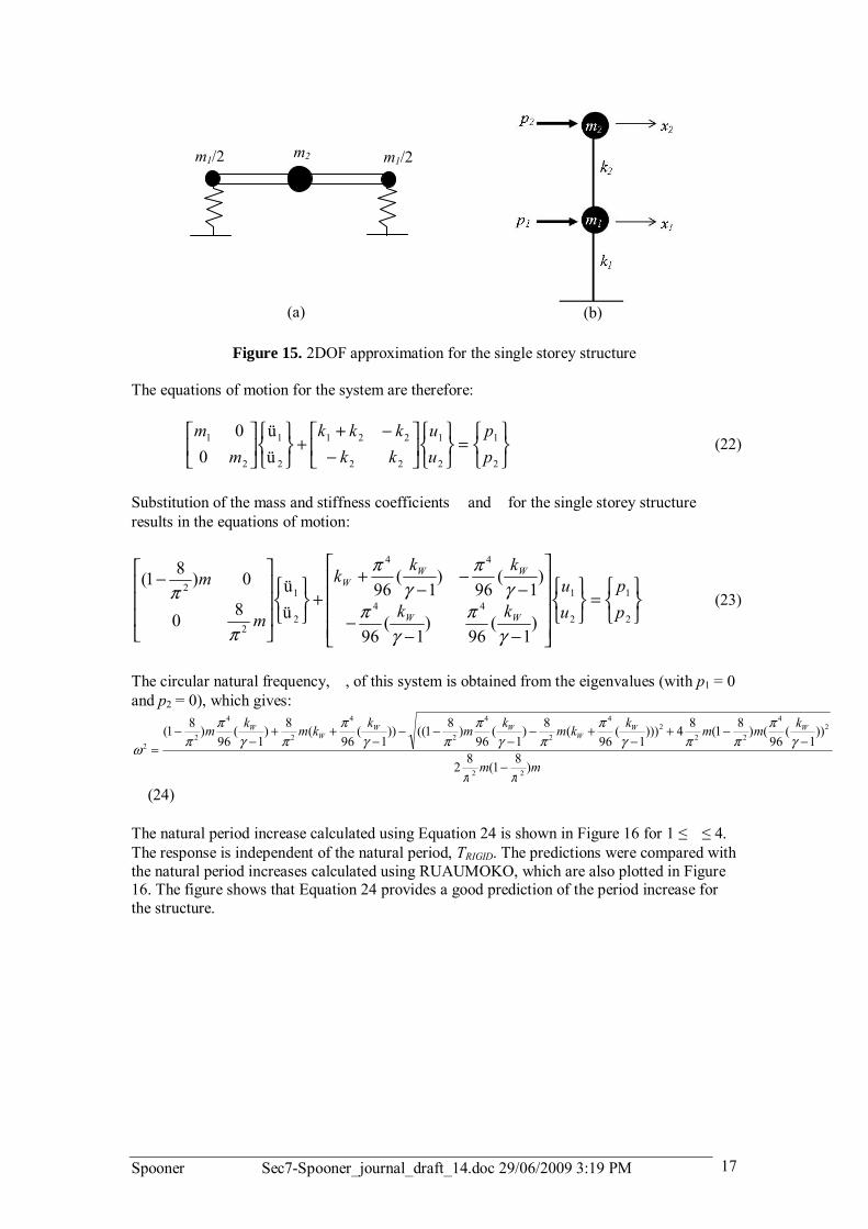
Spooner Sec7-Spooner_journal_draft_14.doc 29/06/2009 3:19 PM 17
Figure 15. 2DOF approximation for the single storey structure
The equations of motion for the system are therefore:
⎭⎬⎫
⎩⎨⎧
=⎭⎬⎫
⎩⎨⎧
⎥⎦
⎤⎢⎣
⎡−
−++
⎭⎬⎫
⎩⎨⎧
⎥⎦
⎤⎢⎣
⎡
2
1
2
1
22
221
2
1
2
1
üü
00
pp
uu
kkkkk
mm
(22)
Substitution of the mass and stiffness coefficients and for the single storey structure results in the equations of motion:
⎭⎬⎫
⎩⎨⎧
=⎭⎬⎫
⎩⎨⎧
⎥⎥⎥⎥
⎦
⎤
⎢⎢⎢⎢
⎣
⎡
−−−
−−
−+
+⎭⎬⎫
⎩⎨⎧
⎥⎥⎥
⎦
⎤
⎢⎢⎢
⎣
⎡ −
2
1
2
144
44
2
1
2
2
)1
(96
)1
(96
)1
(96
)1
(96
üü
80
0)81(
pp
uu
kk
kkk
m
m
WW
WWW
γπ
γπ
γπ
γπ
π
π (23)
The circular natural frequency, , of this system is obtained from the eigenvalues (with p1 = 0 and p2 = 0), which gives:
mm
kmmkkmkmkkmkm WWW
WWW
W
)8
1(8
2
))1
(96
()81(84)))1
(96
(8)1
(96
)81(())1
(96
(8)1
(96
)81(
22
24
222
4
2
4
2
4
2
4
22
ππ
γπ
ππγπ
πγπ
πγπ
πγπ
πω−
−−+
−+−
−−−
−++
−−
=
(24) The natural period increase calculated using Equation 24 is shown in Figure 16 for 1 ≤ ≤ 4. The response is independent of the natural period, TRIGID. The predictions were compared with the natural period increases calculated using RUAUMOKO, which are also plotted in Figure 16. The figure shows that Equation 24 provides a good prediction of the period increase for the structure.
m2 m1/2 m1/2
(a) (b)

Spooner Sec7-Spooner_journal_draft_14.doc 29/06/2009 3:19 PM 18
0
10
20
30
40
50
60
70
80
90
1 1.5 2 2.5 3 3.5 4Static Displacement Ratio, γ
Nat
ural
Per
iod
Incr
ease
, TIN
CR
(%) Ruaumoko
2DOF Solution
Figure 16. Comparison of Period Increase Response for the 2DOF Solution and
RUAUMOKO Output for a Flexural Beam (c) Two Degree-of-Freedom Model Peak Displacement Estimation The peak displacement for a SDOF system under lateral force, δTOT,SDOF, is given by:
WWW
FWFWSDOFTOT γδγδ
δδδδδδ =−+=+=+= ))1(1()1(, (25)
For a MDOF system, the SDOF mass displacement has to be multiplied by the participation factor, Γ. This is equal to 4/π as described in Equation 15. The peak displacement, δTOT,MDOF, for a MDOF system is therefore given by:
))1(1()( ,, −Γ+=−Γ+=Γ+= γδδδδδδδ WWSDOFTOTWFWMDOFTOT (26) Since RATIOMAX ,δ is the peak displacement response as a fraction of the response considering a rigid diaphragm, and for a rigid diaphragm, the peak displacement, δTOT, is equal to the wall displacement, δW,RIGID. The ratio of peak displacement to rigid wall displacement is therefore:
))1(1(,,
,, −γΓ+
δδ
=δ
δ=δ
RIGIDW
W
RIGIDW
MDOFTOTRATIOMAX (27)
Changes in wall shear force are attributed to changes in spectral acceleration. For a given change in period, the change in shear force and therefore wall displacement can be predicted from the spectral acceleration plot shown in Figure 6. The ratio of wall displacement, δW, to rigid wall displacement, δW,RIGID, in the above equation can therefore be approximated by the change in spectral acceleration. From Figure 6, for large period structures, the spectral acceleration decreases with flexibility, therefore δW,/δW,RIGID is less than unity so it is conservative to assume δW,/δW,RIGID is unity for these structures. This is the assumption made in Figure 17 which shows that the predicted and analytical responses for the single storey elastic structures were similar. For short period structures, the solution slightly underestimated the response, and for longer period structures, the prediction generally overestimated the response as would be expected when δW,/δW,RIGID is assumed to be unity.

Spooner Sec7-Spooner_journal_draft_14.doc 29/06/2009 3:19 PM 19
0
1
2
3
4
5
6
7
1 1.5 2 2.5 3 3.5
Static Displacement Ratio, γ
Peak
Dis
plac
emen
t Inc
reas
e, δ
MA
X,R
ATI
O2DOF solution
Ruaumoko Response
TRIGID
0.1s
1.0s
0.5s
Figure 17. Comparison of displacement response for the 2DOF solution and RUAUMOKO
output for TRIGID = 0.1s, 0.5s and 1.0s
5.3 Approximate Response Prediction The natural period is T = 2 / for a 2DOF system where is from Equation 24. However, evaluation of this equation is tedious, so a simpler method was developed to use when designing structures with any number of storeys. This method involved computing the change in spectral displacement for a given change in period. Chopra (2000) gives the natural period of the fundamental mode for a beam with distributed mass, TBEAM:
EILTBEAM
42 ρπ
= (28)
The Canadian Steel Code provisions for floor vibrations calculate the period of a floor system as the sum of the period of the floor slab and the supporting girders (CAN/CSA-S136, 1994). Applying this idea, the period of the structure, TSYS, was calculated by adding the periods of the rigid structure and the most rigid floor element in the structure, TWALL and TFLOOR respectively:
FLOORWALLSYS TTT += (29) Using Equation 29, the change in period was calculated over a range of flexibilities, γ, and corresponding changes in spectral displacement interpolated from Figure 6b. It may be seen in Figure 18 that this method overestimates the peak displacement for all periods considered.

Spooner Sec7-Spooner_journal_draft_14.doc 29/06/2009 3:19 PM 20
0
1
2
3
4
5
6
7
8
1 1.5 2 2.5 3
Static Displacement Ratio, γ
Peak
Dis
plac
emen
t Inc
reas
e, δ
MA
X,R
ATI
OSimple Method
Ruaumoko
TRIGID
0.1s
1.0s
0.5s
Figure 18. Displacement Increase for Simple Method Solution and RUAUMOKO Output for
TRIGID = 0.1s, 0.5s, and 1.0s
6. DESIGN METHODS FOR FLEXIBLE DIAPHRAGMS
6.1. Possible Design Approaches (a) Method One: Period Independent This design check uses the maximum observed response to conservatively estimate the increase in demands for a structure of any period. Based on the observations of earlier chapters, the critical response was for a single storey structure with elastic walls and a rigid period, TRIGID, of 0.1 s. From Figures 5(c) and 5(d), the maximum median increase was 1.4 and 1.7 for shear force and bending moment respectively. The following step by step analysis method may be used for structures which are subject to earthquake excitations. Step 1. Analyse the structure using standard methods and assuming a rigid
diaphragm model to obtain the peak displacements, bending moments and shear forces.
Step 2. Calculate the flexibility ratio, γ, based on the stiffness of the most flexible floor and the walls, using Equation 7.
Step 3. Use the median response for TRIGID = 0.1 s in Figure 5(a), and interpolate the increase in peak displacement, δMAX,RATIO. The maximum displacement is given as TOT,FLEX = TOT,RIGID x δMAX,RATIO.
Step 4. Multiply the peak diaphragm bending moments by 1.7 and peak shear forces by 1.4 to get the design moments and shears respectively.
This method is conservative for multi-storey structures and results in a large amplification of shears and moments. For structures with long natural periods, the shears and moments decreased. Application of the above method to design of real structures could therefore be uneconomical.

Spooner Sec7-Spooner_journal_draft_14.doc 29/06/2009 3:19 PM 21
An alternative design method is to acknowledge that special considerations for short period structures are made in design. That is, these structures are required to be designed for a higher level of acceleration than the actual level as shown in Figure 19. For this reason there is no amplification of shear force and bending moment based on the response of longer period structures in Figures 5(c) and 5(d). The following design step by step methodology will be appropriate for structures which are subject to earthquake excitations. Step 1. Analyse the structure using standard methods and assuming a rigid
diaphragm model to obtain the peak displacements, bending moments and shear forces.
Step 2. Calculate the flexibility ratio, γ, based on the stiffness of the most flexible floor and the walls, using Equation 7.
Step 3. Use the median response for long period structures from Figure 5(a) to estimate the peak displacement, δMAX,RATIO = (1 + 2( ). The maximum displacement is given as TOT,FLEX = TOT,RIGID x δMAX,RATIO.
Step 4. The peak diaphragm bending moments and peak shear forces are taken as those for the rigid diaphragm.
This method is also slightly conservative for multi-storey structures as shown by comparing the δMAX,RATIO with the response in Figure 13. (b) Method Two: Period Dependent An alternative design check is proposed that is less conservative, because the period of the structure is explicitly considered. The method described to develop a simple solution was shown to conservatively estimate the displacement response while considering the period of the structure, so is used to develop this methodology. The following step-by-step methodology is proposed as a less conservative design check for structures which are subject to earthquake excitations. Step 1. Analyse the structure using standard methods and assuming a rigid
diaphragm model to obtain the rigid period, TRIGID, peak displacements, bending moments and shear forces.
Step 2. Given the diaphragm dimensions and properties, use Equation 28 to calculate the period of the floor, TBEAM. Approximate the period of the structure, TFLEX, as:
TFLEX = TRIGID + TBEAM (30) Step 3. Use TFLEX and TRIGID to obtain the changes in spectral acceleration and
spectral displacement from the response spectra. Step 4. The change in spectral displacement is the change in peak displacement,
δMAX,RATIO. If the spectral acceleration increases, the shears and moments should be amplified accordingly.
When response spectra and the equivalent static method of NZS 1170.5 are used, no amplification of forces and moments is necessary. This is because the spectral acceleration plot is truncated at the peak, as shown in Figure 19, to give small period structures the maximum spectral acceleration. Following the code spectra, forces will either be the same or less, as a diaphragm becomes more flexible.

Spooner Sec7-Spooner_journal_draft_14.doc 29/06/2009 3:19 PM 22
Figure 19. NZS 1170.5 approximation to response spectra for equivalent static design (c) Method Three: Using 2DOF Model The approach described to derive Figure 17 above in Section 5.2 was the shown to be appropriate for the 2DOF model. However, due to the difficulty in computing the parameters involved, and difficulty of applying the method to multi-storey structures, it is not recommended as a design method. 6.2 Design Example For the structure shown in Figure 20, the fundamental period considering a rigid diaphragm is 0.14 s. Due to the dimensions of the diaphragm both shear and flexural stiffness are considered and appropriately combined to obtain the total floor stiffness.
Figure 20. Plan and Properties of Example Structure
Method 1: Step 1. The structure is subject to an earthquake which produces a total displacement
of 6.34 mm when the diaphragm is rigid. Any method satisfying code requirements can be used for this displacement prediction. The corresponding shear force and bending moment are 452 kN and 2417 kNm.
Step 2. The flexibility ratio, γ, based on the stiffness of the floor and the walls is 1.20.
Step 3. From the T = 0.1s plot in Figure 5(a), the increase in peak displacement is approximately 1.4, giving a total displacement of 8.7 mm.
Step 4. The shear force is multiplied by 1.4 to get 632 kN, and the bending moment by 1.7 to get 4109 kNm.
Method 2: Step 1. The same rigid diaphragm displacements, forces and moments are used as the
previous design check. Step 2. Using Equation 28, the period of the floor diaphragm is 0.11 s. Adding the
period of the floor and walls gives 0.25 s.
Actual Spectra
Design Spectra
Period, T
Spectral Acceleration

Spooner Sec7-Spooner_journal_draft_14.doc 29/06/2009 3:19 PM 23
Step 3. From Figure 6, the spectral acceleration at this period is 1.42 times the rigid diaphragm value, and spectral displacement is 3.05 times the rigid diaphragm value.
Step 4. The corresponding peak displacement is 19.3 mm and the shear force and bending moment are 642 kN and 3432 kNm for the flexible diaphragm structure.
The design actions obtained from the two methods are compared against the median time history analysis results for the 20 records in Table 1. The first method better predicts displacement and shear, but is worse than the second method at predicting moment. Based on the previous discussion, Method 1 is likely to be very conservative when predicting the demands of multi-storey structures.
Table 1. Prediction of Key Parameters due to Diaphragm Flexibility Method: MAX (mm) VMAX (kN) MMAX (kNm) Time-history 11.2 459 3533 Method 1 8.7 632 4109 Method 2 19.3 642 3432
CONCLUSIONS
Analyses of a range of simple structures were carried out to evaluate the earthquake response of flexible diaphragm structures. The major findings include the following:
1. The change in demand due to diaphragm flexibility was investigated for a range of simple single story structures that were subject to a suite of earthquake ground motion records. The most significant demands were considered to be the mid-span diaphragm displacements and bending moments and the bracing wall shear forces. These demands were independent of the structure dimensions and material properties but were dependent on the period for a rigid floor diaphragm, TRIGID, and the diaphragm flexibility ratio, . The demands were also found to vary with period in response to the spectra shape.
2. The behaviour of the frame did not seem to be significantly affected by whether the diaphragm flexibility was predominantly due to either shear or flexural deformations.
3. Inelastic bracing walls produced demands that were comparable or smaller than those observed with elastic structures.
4. Additional bracing walls and segmented diaphragms produced comparable or smaller increases in demands than that those observed with the simple structure.
5. Simple multi-storey structures exhibited a comparable or smaller increase in demands than those observed with the single storey simple structures.
6. Models were developed to predict the responses. Simple design recommendations were proposed to account for diaphragm flexibility and a design example was provided.

Spooner Sec7-Spooner_journal_draft_14.doc 29/06/2009 3:19 PM 24
REFERENCES Barron, J. M. and Hueste, M. B. D. (2004). Diaphragm Effects in RectangularReinforced
Concrete Buildings. ACI Structural Journal, Vol 101, no. 5,pp. 615-624. Cambridge Advanced Dictionary Online,
http://dictionary.cambridge.org/define.asp?key=68042&dict=CALD Building Seismic Safety Council (2003). NEHRP Recommended Provisions and Commentary
for Seismic Regulations for New Buildings and Other Structures. 2003 Edition, FEMA 450. http://www.fema.gov/library/viewRecord.do?id=2020
Carr, A. J. (2007). Ruaumoko User Manuals. Civil Engineering, University of Canterbury, Christchurch
Chopra, A. K. (2000). Dynamics of Structures: Theory and Applications to Earthquake Engineering. Prentice Hall, pp. 844
Clough, R. W. and Penzien, J. (1993). Dynamics of Structures. McGraw-Hill, pp. 738 CAN/CSA 136-94. (1994). Cold Formed Steel Structural Members. Canadian Standards
Association, Rexdale, Ontario, Canada Fleischman, R. B. and Farrow, K. T. (2001). Dynamic behaviour of perimeter lateral-system
structures with flexible diaphragms. Earthquake Engineering and Structural Dynamics, Vol. 30, no. 5, pp. 745-763.
Fleischman, R. B. and Farrow, K. T. (2003). Seismic Design Recommendations for Precast Concrete Diaphragms in Long Span Floor Construction. PCI Journal, Vol. 48, no. 6, pp. 46-62.
Gulay, G., Ayranci, M. and Sahbaz, U. (2006). A Study on Seismic Resistance of R/C Multi-Storey Buildings with Slab Irregularity. 100th Anniversary Earthquake Conference.
Iverson, J. K. and Hawkins, N. M. (1994). Performance of Precast/Prestressed Concrete Building Structures during the Northridge Earthquake. PCI Journal, Vol. 39, no. 2, pp. 38-55.
Lee, H. J., Aschheim, M A. and Kuchma, D. (2006). Interstorey Drift Estimates for Low-Rise Flexible Fiaphragm Structures. Engineering Structures. Vol. 29, no. 7, pp. 1277-1295.
Lee, H. J., Kuchma, D. and Ashheim, M. A. (2006). Strength-Based Design of Flexible Diaphragms in Low-Rise Structures Subjected to Earthquake Loading. Engineering Structures. Vol 29, no. 7, pp. 1277-1295.
Luco, N. (2002). Probabilistic Seismic Demand Analysis, SMRF Connection Fractures and Near Fault Effects. PhD Thesis, Stanford University.
NZS 1170.5 (2004). Structural Design Action, Part 5: Earthquake Actions. Standards New Zealand, pp. 81
NZS 3101 (2006). Concrete Structures Standard. Standards New Zealand, pp. 685 Park, R. and Paulay, T. (1975) Reinforced Concrete Structures. Wiley, New York, pp. 786 Paquette, J., Bruneau, M. and Brzev, S. (2004). Seismic Testing of Repaired Unreinforced
Masonry Building having Flexible Diaphragm. Journal of Structural Engineering, Vol 130, no. 10, pp. 1487-1496.
SAC Steel, (2002). Suites of Earthquake Ground Motions for Analysis of Steel Moment Frame Structures. <http://nisee.berkeley.edu/data/strong_motion/sacsteel/motions/la10in50yr.html>. Viewed 16 July 2008
SEAOC (1999). Recommended Lateral FOrc Requirements and Commentary”, Seismology Committee, Structural Engineers Association of California. Seventh Edition.
Singh, J. (2008). Vertical Acceleration Effects on Structural Performance. Undergraduate Project, Civil Engineering, University of Canterbury, Christchurch.
Spooner, M.S. (2008). Quantifying the Dynamic Response of Flexible Floor Diaphragms. Undergraduate Project, Civil Engineering, University of Canterbury, Christchurch
Sullivan T. J. (2006). “Floor Behaviour in Frame-Wall Structures”, Chapter 9 of PhD Thesis, Pavia, Italy, 2006.

Spooner Sec7-Spooner_journal_draft_14.doc 29/06/2009 3:19 PM 25
Timoshenko, S. P. (1922). On the Transverse Vibrations of Bars of Uniform Cross-Section. Philosophical Magazine, no. 43, pp. 125–131.

CHAPTER 8. SUMMARY OF RECOMMENDATIONS

CHAPTER 8. SUMMARY OF RECOMMENDATIONS
A. Relationships between Irregularity and Increased Drift
The equations below give an estimate of the likely median increase in demand for critical structures with the irregularity at the critical location which are designed by the NZS1170.5 Equivalent Static Method. This information should give designers a better understanding of the influence of irregularity and more confidence in their designs.
1) Mass irregularity
Drift demand = (Regular structure drift demand) x (1 + 0.15 (MR – 1))where MR is the mass ratio at one storey relative to that of a neighbouring storey
2) Stiffness-strength irregularity (constant storey height)
Drift demand = (Regular structure drift demand) x (1 + 0.4 (SMF – 1)) where SMF > 1.0
Drift demand = (Regular structure drift demand) x (1 + 1.6 (1 – SMF)) where SMF < 1.0where SMF is the stiffness modification factor which is defined as the stiffness of one storey relative to that of the neighbouring storey.
The above two equations are based on the responses of the structures having storey stiffness and strength varying equally by the same amount (SMF).
3) Stiffness-strength irregularity (changing storey height)
Drift demand = (Regular structure drift demand) x (1 + |IHR – 1|)where IHR is the interstorey height ratio which is defined as the ratio of modified interstorey height to the initial interstorey height.
The above equation is based on the responses of the structures having only the storey stiffness modified due to a change in the storey height.
4) Torsional irregularity
In order to limit the total deformation including torsion to less than % of the deformation ignoring torsion, the rotational stiffness, JR,, provided by the out-of-plane and in-plane walls should not exceed that given in the equation below. Parameters are described in Chapter 6:
JR, Vdes . eR xi ( -1) CM
5) Diaphragm Flexibility Effects
Forces are not generally increased due to diaphragm flexibility. However, displacements are. The increase in displacement is given by:
Displacement demand = (Regular structure displacement demand) x (1 + 2()
B. Irregularity Limits Based on a 10% Increase in Drift
If irregularity limits are desired, then a specified level of drift increase should be specified. This can be developed for any strength increase. In the example below, a 10% increase in the drift is considered with the equations in section A above.
1) Mass irregularity
The maximum mass ratio, MR, is 67% above the regular mass level.
This compares with the allowable change of 50% in clause 4.5.1.1 of NZS1170.5. This value of 50% corresponds to a change in response of 1.075 times for a structure designed to show the most effect of irregularity with the irregularity at the critical level according to the equation of section A.
2) Stiffness-strength irregularity (constant storey height)
The stiffness modification factor, SMF, for a change in the properties of one storey relative to the other stories must lie in the range of is -6% to +25% that of the storey above. In this model every floor has the same strength to stiffness ratio and the storey height at all the levels are kept the same.
NZS1170.5 currently considers strength and stiffness irregularity separately.
The stiffness of a storey is not permitted to be less than 70% of an adjacent story in clause 4.5.1.2 of NZS1170.5. This corresponds to a decrease in stiffness of 30%.
In NZS1170.5. clause 4.5.1.3 the strength is not permitted to be any less than 90% of the strength of the floor above. This corresponds to a decrease in strength of 10%.
Based on this, for structures in which stiffness and strength are proportional at each level, NZS1170.5 limits on strength control, and the expected change in response is expected to be 1.16 times for a critical structure according to the equation in Section A.
3) Stiffness-strength irregularity (changing storey height)
According to section A, a storey height can be modified by any IHR having a magnitude between 0.9 and 1.1.
4) Torsional irregularity
The maximum rotational stiffness, JR,, provided by the out-of-plane and in-plane walls should not exceed that given in the equation below.
JR, Vdes . eR xi CM
NZS1170.5 Clause 4.5.2.3 recommendations are based on elastic considerations and do not consider whether in-plane or out-of-plane walls limit the elastic torsion. It is well known that structures designed using this approach may have significant torsional deformations, especially if only the in-plane walls provide all of the torsional resistance.
5) Diaphragm Flexibility Effects
Displacements may be limited by making less than 1.15. Normally for displacements such tight limits are not needed. The code recommends < 3 for diaphragms to be considered stiff. This corresponds to a 133% displacement increase for a single storey structure, but significantly less for a multi-storey structure. This displacement increase is due to both floor and wall flexibility, so it does not correspond to an increase in demand on the walls which will generally have a decrease in displacement due to the lower forces entering the structure.
It should be noted that a number of assumptions were made with respect to the equations and values given above. Some subjective assessments were also made. Before using these equations, readers should familiarize themselves with these assumptions, as described in the appropriate chapter.
C. A Note to Engineers – How can this Work be Used?
The work was conducted to provide New Zealand engineers with: a. a rational basis for regularity limits for designb. an understanding of the sensitivity of drift response to the magnitude of an irregularity
a) Rational Basis for Irregularity Limits for Design
It is possible to specify an acceptable variation in response and then, using the relationships in Part A, to determine the acceptable level of irregularity. This has been done for a 10% variation in response as shown in Part B, but other levels of variation could also be selected.
The use of a consistent variation for all irregularity types results in consistent recommendations for code irregularity limits to tell the engineer what type of analysis should be used for design.
The consistent and rational approach developed above will be promoted for incorporation into the NZ loadings standard “NZS1170.5 – Structural Design Actions – Earthquake Actions – New Zealand”, based on discussion with engineers about an acceptable level of variation.
b) Sensitivity of Behaviour to Irregularity
The variation in response as a function of the magnitude of irregularity, as specified in Part A, is useful for designers to:
a) Perform a rapid preliminary design of a structure with irregularity. b) To tell the client whether the structure can be built with an irregularity modification at a
client-engineer meeting.c) Perform a rapid check of structures which have been designed with more complex analysis
methods. d) Better consider the required capacity. In probabilistic performance based earthquake
engineering, or in code development, the variation in response due to irregularity may be used to provide better estimates of the likely demands on elements of actual structures. This knowledge is important in determining the required capacity of a member.
e) Develop more confidence in their designs because they are aware of the sensitivity to the amount of irregularity.

CHAPTER 9. OPPORTUNITIES FOR FURTHER WORK

CHAPTER 9. OPPORTUNITIES FOR FURTHER WORK
As with any study, there are further opportunities for investigation to improve and refine knowledge. Some activities which would further refine the studies described here are:
a) Structures with several types of irregularity
The work conducted in this study evaluates the effect of one type of irregularity at a time, except when strength and stiffness were considered where there is an obvious correlation between these two types of irregularity. It is possible that torsional irregularity may occur in a structure which also has vertical stiffness-strength irregularity. Other combinations of irregularity are also possible. Structures with multiple irregularities may perform worse than those described here.
b) Evaluate flexural, rather than shear, type structures.
It would be useful to perform a more advanced study of structures which consist of structural walls, which perform in a flexural, rather than in a shear, mode. Such wall structures have behaved exceptionally well in the past. In fact, Mark Fintel indicates that based on damage observations in past earthquakes, wall structures all behaved well. This includes those without necessarily “proper” design.
c) Structures designed using other analysis methods
The work conducted in this study indicates that the Equivalent Static Method is reasonably robust, but there is a change in response for some structures with different amounts of irregularity. Other more sophisticated methods, such as the linear dynamic methods, or non-linear pushover methods, are likely to be more accurate and less sensitive to inelasticity. However, the criteria for the static procedure is not severe, so it is likely that results from other methods will be even less severe. For this reason the likely incremental change in response equations is unlikely to have a significant effect on the design.


