
Ph~:1s:p note
cc:
and ModelingChemical Engineers
Mark E.. DavisVirginia Polytechnic Institute and State University
New York ChichesterJohn Wiley &.. Sons
Brisbane Toronto Singapore
Copyright © 1984, by John Wiley & Sons, Inc.
All rights reserved. Published simultaneously in Canada.
Reproduction or translation of any part ofthis work beyond that permitted by Sections107 and 108 of the 1976 United States CopyrightAct without the permission of the copyrightowner is unlawful. Requests for permissionor further information should be addressed tothe Permissions Department, John Wiley & Sons.
Library of Congress Cataloging in Publication Data:
Davis, Mark E.Numerical methods and modeling for chemical
engineers.
Bibliography: p.Includes index.
1. Chemical engineering-Mathematical models.2. Differential equations. 1. Title.
TP155.D33 1984ISBN 0-471-88761-7
660.2'8'0724 83-21590
Printed in the United States of America
10 9 8 7 6 5 4 3 2 1

To Mary Margaret
Preface
This book is an introduction to the quantitative treatment of differential equations that arise from modeling physical phenomena in the area of chemicalengineering. It evolved from a set of notes developed for courses taught atVirginia Polytechnic Institue and State University.
An engineer working on a mathematical project is typically not interestedin sophisticated theoretical treatments, but rather in the solution of a model andthe physical insight that the solution can give. A recent and important tool inregard to this objective is mathematical software-preprogrammed, reliablecomputer subroutines for solving mathematical problems. Since numerical methods are not infallible, a "black-box" approach of using these subroutines can bedangerous. To utilize software effectively, one must be aware of its capabilitiesand especially its limitations. This implies that the user must have at least anintuitive understanding of how the software is designed and implemented. Thus,although the subjects covered in this book are the same as in other texts, thetreatment is different in that it emphasizes the methods implemented in commercial software. The aim is to provide an understanding of how the subroutineswork in order to help the engineer gain maximum benefit from them.
This book outlines numerical techniques for differential equations that eitherillustrate a computational property of interest or are the underlying methods ofa computer software package. The intent is to provide the reader with sufficientbackground to effectively utilize mathematical software. The reader is assumedto have a basic knowledge of mathematics, and results that require extensivemathematical literacy are stated with proper references. Those who desire to
vii
viii Preface
delve deeper into a particular subject can then follow the leads given in thereferences and bibliographies.
Each chapter is provided with examples that further elaborate on the text.Problems at the end of each chapter are aimed at mimicking industrial mathematics projects and, when possible, are extensions of the examples in the text.These problems have been grouped into two classes:
Class 1: Problems that illustrate direct numerical application of the formulasin the text.
Class 2: Problems that should be solved with software of the type describedin the text (designated by an asterisk after the problem number).
The level of this book is introductory, although the latest techniques arepresented. The book can serve as a text for a senior or first-year graduate levelcourse. At Virginia Polytechnic Institute and State University I have successfullyused this material for a two-quarter sequence of first-year graduate courses. Inthe first quarter ordinary differential equations, Chapter 1 to 3, are covered.The second quarter examines partial differential equations using Chapters 4 and5.
I gratefully acknowledge the following individuals who have either directlyor indirectly contributed to this book: Kenneth Denison, Julio Diaz, Peter Mercure, Kathleen Richter, Peter Rony, Layne Watson, and John Yamanis. I amespecially indebted to Graeme Fairweather who read the manuscript and provided many helpful suggestions for its improvement. I also thank the Departmentof Chemical Engineering at Virginia Polytechnic Institute and State Universityfor its support, and I apologize to the many graduate students who sufferedthrough the early drafts as course texts. Last, and most of all, my sincerestthanks go to Jan Chance for typing the manuscript in her usual flawless form.
I dedicate this book to my wife, who uncomplainingly gave up a portion ofher life for its completion.
Mark E. Davis
Chapter 1 Initial-Value Problems forOrdinary Differential Equations 1
Introduction 1Background 1
Explicit Methods 3Stability 8Runge-Kutta Methods 11Implicit Methods 19Extrapolation 11Multistep Methods 14High-Order Methods Based on Knowledge 18of allayStiffness 19Systems of Differential E.quations 31Step-Size Strategies 36Mathematical Software 37Problems 44References 49Bibliography 51
ix
x
Chapter 2
Chapter 3
Boundary-Value Problemsfor Ordinary DifferentialEquations: Discrete Variable Methods
IntroductionBackgroundInitial-Value Methods
Shooting MethodsMultiple ShootingSuperposition
finite Difference MethodsLinear Second-Order EquationsFlux Boundary ConditionsIntegration MethodNonlinear Second-Order EquationsFirst-Order SystemsHigher-Order Methods
Mathematical SoftwareProblemsReferencesBibliography
Boundary-Value Problemsfor Ordinary DifferentialEquations: finite Element Methods
IntroductionBackgroundPiecewise Polynomial FunctionsThe Galerkin Method
Nonlinear EquationsInhomogeneous Dirichletand Flux Boundary ConditionsMathematical Software
CollocationMathematical Software
ProblemsReferencesBibliography
Contents
53
5353545463656768717579838587919395
97
979799104109
110111112119123125126
Contents
Chapter 4
Chapter 5
Parabolic Partial DifferentialEquations in One Space Variable
IntroductionClassification ofPartial Differential EquationsMethod of Linesfinite Differences
Low-Order Time ApproximationsThe Theta MethodBoundary and Initial ConditionsNonlinear EquationsInhomogeneous MediaHigh-Order Time Approximations
Finite ElementsGalerkinCollocation
Mathematical SoftwareProblemsReferencesBibliography
Partial DifferentialEquations in Two Space Variables
127
127
127128130130133135140142147154154158162167172174
177
Introduction 177Elliptic PDEs-Finite Differences 177
Background 177Laplace's Equation in a Square 178
Dirichlet Problem 178Neumann Problem 179Robin Problem 180
Variable Coefficients and Nonlinear Problems 184Nonuniform Grids 185Irregular Boundaries 190
Dirichlet Condition 190Normal Derivative Conditions 191
Elliptic PDEs-finite Elements 192Background 192Collocation 194Gakr~n 200
xli
Appendices
Parabolic PDEs in Two Space VariablesMethod of LinesAlternating Direction Implicit Methods
Mathematical SoftwareParabolicsElliptics
ProblemsReferencesBibliography
Contents
211211212214215219222224227
A: Computer Arithmetic and Error Control 229Computer Number System 229Normalized Floating Point Number System 230Round-Off Errors 230
B: Newton's Method 235C: Gaussian Elimination 237
Dense Matrix 237Tridiagonal Matrix 241
D: B-Splines 243E: Iterative Matrix Methods 247
Appendix References 249
Author Index 251
Subject Index 255
Numerical Methodsand Modeling
for Chemical Engineers
Initlal..Value Problems for OrdinaryDifferential Equations
INTRODUCTION
The goal of this book is to expose the reader to modern computational tools forsolving differential equation models that arise in chemical engineering, e.g.,diffusion-reaction, mass-heat transfer, and fluid flow. The emphasis is placedon the understanding and proper use of software packages. In each chapter weoutline numerical techniques that either illustrate a computational property ofinterest or are the underlying methods of a computer package. At the close ofeach chapter a survey of computer packages is accompanied by examples oftheir use.
BACKGROUND
Many problems in engineering and science can be formulated in terms of differential equations. A differential equation is an equation involving a relationbetween an unknown function and one or more of its derivatives. Equationsinvolving derivatives of only one independent variable are called ordinary differential equations and may be classified as either initial-value problems (IVP)or boundary-value problems (BVP). Examples of the two types are:
IVP: y" = -yx (l.la)
yeO) = 2, y'(O) 1 (l.lb)
BVP: y" = -yx (l.2a)
yeO) = 2, y(l) = 1 (l.2b)
1
2 Initial-Value Problems for Ordinary Differential Equations
where the prime denotes differentiation with respect to x. The distinction between the two classifications lies in the location where the extra conditions [Eqs.(LIb) and (1.2b)] are specified. For an IVP, the conditions are given at thesame value of x, whereas in the case of the BVP, they are prescribed at twodifferent values of x.
Since there are relatively few differential equations arising from practicalproblems for which analytical solutions are known, one must resort to numericalmethods. In this situation it turns out that the numerical methods for each typeof problem, IVP or BVP, are quite different and require separate treatment. Inthis chapter we discuss IVPs, leaving BVPs to Chapters 2 and 3.
Consider the problem of solving the mth-order differential equation
y(m) = f(x, Y, y', y", ... , y(m-1») (1.3)
with initial conditions
y(xo) = Yo
y'(XO) = yb
y(m-1) (XO) = Y6m- 1)
where f is a known function and Yo, yb, ... ,Y6m-1) are constants. It is customary
to rewrite (1.3) as an equivalent system of m first-order equations. To do so,we define a new set of dependent variables Y1(X), Yz(x), ... , Ym(x) by
Yl = Y
Yz = Y'
Y3 = y"
Ym = y(m-1)
(1.4)
and transform (1.3) into
Y;' = Yz
y~ = Y3
= f1(X, Yl, Yz, , Ym)
= fz(x, Y1' Yz, , Ym) (1.5)
y:r, = f(x, Yv Yz, ... , Ym) = fm(x, Yv Yz, ... , Ym)
with
Y1(XO) = Yo
yzCxo) = yb
Explicit Methods
In vector notation (1.5) becomes
y'(x) = rex, y)
y(xo) = Yo
where
3
(1.6)
[
heX)]y(x) = Y2~X) ,
Ym(X)[
fleX, y)]rex, y) = f2(X; y) ,
fm(x, y)[
Yo]Y
_ ybo - .
y~m'-l)
It is easy to see that (1.6) can represent either an mth-order differentialequation, a system of equations of mixed order but with total order of m, or asystem of m first-order equations. In general, subroutines for solving IVPs assume that the problem is in the form (1.6). In order to simplify the analysis, webegin by examining a single first-order IVP, after which we extend the discussionto include systems of the form (1.6).
Consider the initial-value problem
y' = f(x, y), Y(Xo) = Yo (1.7)
We assume that aflay is continuous on the strip Xo ~ x ~ XN' thus guaranteeingthat (1.7) possesses a unique solution [1]. If y(x) is the exact solution to (1.7),its graph is a curve in the xy-plane passing through the point (xo, Yo). A discretenumerical solution of (1.7) is defined to be a set of points [(Xi' u;)]~o, whereUo = Yo and each point (Xi' u;) is an approximation to the corresponding point(Xi' Y(Xi)) on the solution curve. Note that the numerical solution is only a setof points, and nothing is said about values between the points. In the remainderof this chapter we describe various methods for obtaining a numerical solution[(Xi' Ui)]~O'
EXPLICIT METHODS
We again consider (1.7) as the model differential equation and begin by dividingthe interval [xo, XN] into N equally spaced subintervals such that
Xi = Xo + ih, i = 0, 1,2, ... , N
(1.8)
The parameter h is called the step-size and does not necessarily have to beuniform over the interval. (Variable step-sizes are considered later.)
4 Initial-Value Problems for Ordinary Differential Equations
If y(x) is the exact solution of (1.7), then by expanding y(x) about thepoint Xi using Taylor's theorem with remainder we obtain:
Y(Xi+1) = y(xi) + (Xi+1 - xi)y'(Xi)
+ (X i + 12~ xy y"(~J,
The substitution of (1.7) into (1.9) gives
(1.9)
(1.10)
The simplest numerical method is obtained by truncating (1.10) after the secondterm. Thus with Ui = y(xJ,
Ui+1 = Ui + hf(xi , uJ,
Uo = Yo
i = 0, 1, ... , N - 1, (1.11)
This method is called the Euler method.By assuming that the value of Ui is exact, we find that the application of
(1.11) to compute Ui+1 creates an error in the value of Ui+1. This error is calledthe local truncation error, ei+1. Define the local solution, z(x), by
Z'(X) = f(x, z), Z(Xi) = Ui (1.12)
An expression for the local truncation error, ei+1 = Z(Xi+1) Ui+1' can beobtained by comparing the formula for Ui+1 with the Taylor's series expansionof the local solution about the point Xi. Since
z(xi + h) = z(xi) + hf(Xi' z(xi» + ~~ z"(~J
or
Z(Xi + h) = Ui + hf(Xi' uJ + ~~ Z"(~i)'
it follows that
(1.13)
ei+1 = ~~ Z"(~i) = 0(h2) (1.14)
The notation O( ) denotes terms of order ( ), i.e. ,f(h) = O(hL) if If(h)1 ~ Ah l
as h~ 0, where A and I are constants [1]. The global error is defined as
(1.15)
and is thus the difference between the true solution and the numerical solutionat X = Xi+1. Notice the distinction between ei+1 and c; i+1. The relationshipsbetween ei+1 and c; i+1 will be discussed later in the chapter.
Explicit Methods
We say that a method is pth-order accurate if
ei+l = 0(hP+ 1)
5
(1.16)
and from (1.14) and (1.16) the Euler method is first-order accurate. From theprevious discussions one can see that the local truncation error in each step canbe made as small as one wishes provided the step-size is chosen sufficiently small.
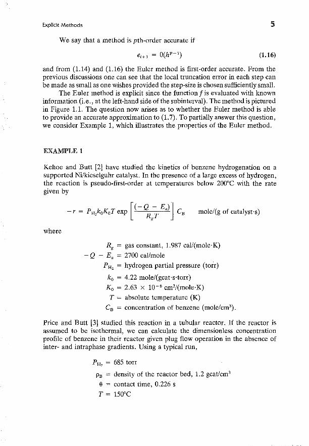
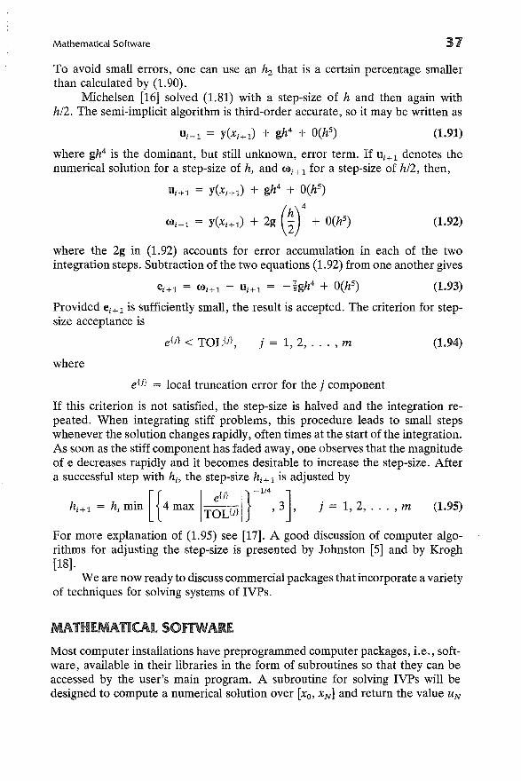
The Euler method is explicit since the function f is evaluated with knowninformation (i.e., at the left-hand side of the subinterval). The method is picturedin Figure 1.1. The question now arises as to whether the Euler method is ableto provide an accurate approximation to (1.7). To partially answer this question,we consider Example 1, which illustrates the properties of the Euler method.
EXAMPLE 1
Kehoe and Butt [2] have studied the kinetics of benzene hydrogenation on asupported Ni/kieselguhr catalyst. In the presence of a large excess of hydrogen,the reaction is pseudo-first-order at temperatures below 200°C with the rategiven by
mole/(g of catalyst·s)
where
Rg = gas constant, 1.987 cal/(mole'K)
- Q - Ea = 2700 cal/mole
PH2 = hydrogen partial pressure (torr)
ko = 4.22 mole/(gcat·s·torr)
Ko = 2.63 X 10- 6 cm3/(mole'K)
T = absolute temperature (K)
CB = concentration of benzene (mole/cm3).
Price and Butt [3] studied this reaction in a tubular reactor. If the reactor isassumed to be isothermal, we can calculate the dimensionless concentrationprofile of benzene in their reactor given plug flow operation in the absence ofinter- and intraphase gradients. Using a typical run,
PH2 = 685 torr
PB = density of the reactor bed, 1.2 gcat/cm3
e = contact time, 0.226 s
T = 150°C
6
SLOPE =f (xO'YO)
y y o
fiGURE. 1.1 Euler method.
SOLUTION
Initial-Value Problems for Ordinary Differential Equations
y(x)
(X3'U3)III SLOPE=f(x2,u2)IIIIII
Define
C~ = feed concentration of benzene (mole/cm3)
z = axial reactor coordinate (cm)
L reactor length
y dimensionless concentration of benzene (CB / C~)
x = dimensionless axial coordinate (z/L).
The one-dimensional steady-state material balance for the reactor that expressesthe fact that the change in the axial convection of benzene is equal to the amountconverted by reaction is
with
C~ at x oSince e is constant,
: = - PBePH2koKoT exp [( - ~g-;' Ea)] y
Let
Explicit Methods
Using the data provided, we have <!>
equation becomes
7
21.6. Therefore, the material balance
dy = -21.6ydx
with
y 1 at x = 0
and analytical solution
y = exp (-21.6x)
Now we solve the material balance equation using the Euler method [Eq. (1.11)]:
where
U i + 1 = U i - 21.6hu;, i = 0, 1, 2, ... , N - 1
h=lN
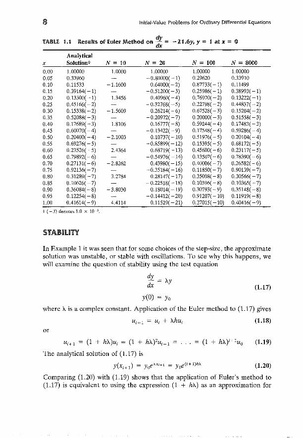
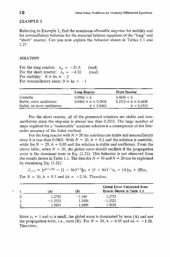
Table 1.1 shows the generated results. Notice that for N = 10 the differences between the analytical solution and the numerical approximation increasewith x. In a problem where the analytical solution decreases with increasingvalues of the independent variable, a numerical method is unstable if the globalerror grows with increasing values of the independent variable (for a rigorousdefinition of stability, see [4]). Therefore, for this problem the Euler method isunstable when N = 10. For N = 20 the global error decreases with x, but thesolution oscillates in sign. If the error decreases with increasing x, the methodis said to be stable. Thus with N = 20 the Euler method is stable (for thisproblem), but the solution contains oscillations. For all N > 20, the method isstable and produces no oscillations in the solution.
From a practical standpoint, the "effective" reaction zone would be approximately 0 ~ x ~ 0.2. If the reactor length is reduced to 0.2L, then a morerealistic problem is produced. The material balance equation becomes
dy = -4.32ydx
y = 1 at x = 0
Results for the "short" reactor are shown in Table 1.2. As with Table 1.1, wesee that a large number of steps are required to achieve a "good" approximationto the analytical solution. An explanation of the observed behavior is providedin the next section.
Physically, the solutions are easily rationalized. Since benzene is a reactant,thus being converted to products as the fluid progresses toward the reactor outlet(x = 1), Y should decrease with x. Also, a longer reactor would allow for greaterconversion, i.e., smaller y values at x = 1.
(1.17)
8 Initial-Value Problems for Ordinary Differential Equations
TABU 1.1 Results of Euler Method on :: = -21.6y,y = 1 atx = 0
Analyticalx Solutiont N = 10 N = 20 N = 100 N = 8000
0.00 1.00000 1.0000 1.00000 1.00000 1.000000.05 0.33960 - 0.80000( -1) 0.29620 0.339100.10 0.11533 -1.1600 0.64000( -2) 0.87733( -1) 0.114990.15 0.39164( -1) - 0.51200( - 3) 0.25986( -1) 0.38993( -1)0.20 0.13300(-1) 1.3456 oo40960( - 4) 0.76970( -2) 0.13222(-1)0.25 0045166( - 2) - 0.32768( - 5) 0.22798( -2) 0044837( - 2)0.30 0.15338( - 2) -1.5609 0.26214( -6) 0.67528( - 3) 0.15204(-2)0.35 0.52088( -3) -0.20972( -7) 0.20000(-3) 0.51558( - 3)0.40 0.17689(-3) 1.8106 0.16777( -8) 0.59244( -4) 0.17483(-3)0045 0.60070( -4) -0.13422( -9) 0.17548(-4) 0.59286(-4)0.50 0.20400( -4) -2.1003 0.10737( -10) 0.51976( - 5) 0.20104(-4)0.55 0.69276( - 5) - 0.85899( -12) 0.15395( - 5) 0.68172( -5)0.60 0.23526( -5) 204364 0.68719( -13) 0045600( - 6) 0.23117( - 5)0.65 0.79892(-6) -0.54976( -14) 0.13507( - 6) 0.78390(-6)0.70 0.27131( -6) -2.8262 oo43980( - 15) oo40006( - 7) 0.26582( - 6)0.75 0.92136( -7) - 0.35184( -16) 0.11850(-7) 0.90139(-7)0.80 0.31289( -7) 3.2784 0.28147( -17) 0.35098( - 8) 0.30566(-7)0.85 0.10626(-7) - 0.22518( -18) 0.10396( - 8) 0.10365( -7)0.90 0.36084( -8) -3.8030 0.18014( -19) 0.30793(-9) 0.35148( - 8)0.95 0.12254( - 8) -0.14412( -20) 0.91207( -10) 0.11919( - 8)1.00 0.41614( - 9) 404114 0.11529( - 21) 0.27015( -10) 0.40416( - 9)
t ( - 3) denotes 1.0 x 10⁻³,
STABILITY
In Example 1 it was seen that for some choices of the step-size, the approximatesolution was unstable, or stable with oscillations. To see why this happens, wewill examine the question of stability using the test equation
dy = Aydx
yeO) = Yo
where Ais a complex constant. Application of the Euler method to (1.17) gives
Ut+1 = Ut + Ahutor
Ut+l = (1 + hA)Ut = (1 + hA)2Ut _ 1 =
The analytical solution of (1.17) is
y(x t+ 1) = yoeAXi+l = yoe(i+l)hA
(1.18)
(1.19)
(1.20)
Comparing (1.20) with (1.19) shows that the application of Euler's method to(1.17) is equivalent to using the expression (1 + hA) as an approximation for
Stability 9
TABLE. 1.1 Results of Euler Method on dy = -4.31y, Y = 1 at x = 0dx
Analyticalx Solution N = 100 N = 1000 N = 8000
0.0 1.00000 1.00000 1.00000 1.000000.1 0.64921 0.64300 0.64860 0.649130.2 0.42147 0.41345 0.42068 0.421370.3 0.27362 0.26585 0.27286 0.273530.4 0.17764 0.17094 0.17698 0.177560.5 0.11533 0.10992 0.11479 0.115260.6 0.07487 0.07067 0.07445 0.074810.7 0.04860 0.04544 0.04828 0.048560.8 0.03155 0.02922 0.03132 0.031520.9 0.02048 0.01878 0.02031 0.020461.0 0.01330 0.01208 0.01317 0.01328
e Ah . Now suppose that the value Yo is not exactly representable by a machinenumber (see Appendix A), then eo = Yo - Uo will be nonzero. From (1.19),with Uo replaced by Yo - eo,
Ui+1 (1 + h1l.)i+1 (yo - eo)
and the global error (5 i+1 is
(5i+1 = Y(Xi+1) - Ui+1 = yoe(i+1)hA - (1 + hA)i+1 (Yo - eo)
or
(5i+1 = [e(i+1)Ah - (1 + hA)i+1] Yo + (1 + hA)i+1eo (1.21)
Hence, the global error consists of two parts. First, there is an error that resultsfrom the Euler method approximation (1 + hA) for eAh . The second part is thepropagation effect of the initial error, eo. Clearly, if 11 + hAl> 1, this componentwill grow and, no matter what the magnitude of eo is, it will become the dominantterm in (5 i + l' Therefore, to keep the propagation effects of previous errorsbounded when using the Euler method, we require
11 + hAl <s; 1 (1.22)
The region of absolute stability is defined by the set of h (real nonnegative) andAvalues for which a perturbation in a single value Ui will produce a change insubsequent values that does not increase from step to step [4]. Thus, one cansee from (1.22) that the stability region for (1.17) corresponds to a unit disk inthe complex hA-plane centered at ( -1, 0). If Ais real, then
- 2 <S; hA <S; 0 (1.23)
Notice that if the propagation effect is the dominant term in (1.21), the globalerror will oscillate in sign if - 2 <S; hA <S; - 1.
to
EXAMPLE 2
Initial-Value Problems for Ordina'Y Differential Equations
Referring to Example 1, find the maximum allowable step-size for stability andfor nonoscillatory behavior for the material balance equations of the "long" and"short" reactor. Can you now explain the behavior shown in Tables 1.1 and1.2?
SOLUTION
For the long reactor: 'AL = - 21.6For the short reactor: 'As = - 4.32For stability: 0;;,: h'A ;;,: - 2For nonoscillatory error: 0 ;;,: h'A > -1
(real)(real)
UnstableStable, error oscillationsStable, no error oscillations
Long Reactor
0.0926 < h0.0463 ~ h ~ 0.0926
h < 0.0463
Short Reactor
0.4630 < h0.2315 ~ h ~ 0.4630
h < 0.2315
For the short reactor, all of the presented solutions are stable and nonoscillatory since the step-size is always less than 0.2315. The large number ofsteps required for a "reasonably" accurate solution is a consequence of the firstorder accuracy of the Euler method.
For the long reactor with N > 20 the solutions are stable and nonoscillatorysince h is less than 0.0463. With N = 10, h = 0.1 and the solution is unstable,while for N = 20, h = 0.05 and the solution is stable and oscillatory. From theabove table, when N = 20, the global error should oscillate if the propagationerror is the dominant term in Eq. (1.21). This behavior is not observed fromthe results shown in Table 1.1. The data for N = 10 and N = 20 can be explainedby examining Eq. (1.21):
6i+l = [e(i+l)Ah - (1 + h'A)i+l]yo + (1 + h'A)i+leo = (A)yo + (B)eo
For N = 10, h = 0.1 and 'Ah = -2.16. Therefore,
o12
(A)
1.2753-1.3323
1.5624
(B)
-1.1601.3456
-1.5609
Global Error Calculated fromResults Shown in Table 1.1
1.2753-1.3323
1.5624
Since Yo = 1 and eo is small, the global error is dominated by term (A) and notthe propagation term, i.e., term (B). For N = 20, h = 0.05 and 'Ah = -1.08.Therefore,
Runge-Kutta Methods 11
o12
(A)
0.41960.10890.3967 x 10- 1
(B)
-0.080.64 x 10- 2
-0.512 X 10⁻³
Global Error Calculated fromResults Shown in Table 1.1
0.41960.10890.3967 x 10- 1
As with N = 10, the global error is dominated by the term (A). Thus no oscillations in the global error are seen for N = 20.
From (1.19) one can explain the oscillations in the solution for N = 10and 20. If
(1 + hA) < 0
then the numerical solution will alternate in sign. For (1 + hA) to be equal tozero, hA = -1. When N = 10 or 20, hA is less than -1 and therefore oscillationsin the solution occur.
For this problem, it was shown that for the long reactor with N = 10 or20 the propagation error was not the dominant part of the global error. Thisbehavior is a function of the parameter A and thus will vary from problem toproblem.
From Examples 1 and 2 one observes that there are two properties of theEuler method that could stand improvement: stability and accuracy. Implicitwithin these categories is the cost of computation. Since the step-size of theEuler method has strict size requirements for stability and accuracy, a largenumber of function evaluations are required, thus increasing the cost of computation. Each of these considerations will be discussed further in the followingsections. In the next section we will show methods that improve the order ofthe accuracy.
RUNGE·KUTIA METHODS
Runge-Kutta methods are explicit algorithms that involve evaluation of thefunction f at points between Xi and Xi + l' The general formula can be written as
where
v
U i + 1 = U i + 2: wjKjj=1
(1.24)
(1.25)
12 Initial-Value Problems for Ordinary Differential Equations
(1.26)
Notice that if v = 1, WI = 1, and K 1 = hf(x;, u;), the Euler method is obtained.Thus, the Euler method is the lowest-order Runge-Kutta' formula. For higherorder formulas, the parameters w, C, and a are found as follows. For example,if v = 2, first expand the exact solution of (1.7) in a Taylor's series,
Y(Xi+1) = y(x) + hf(x;, y(x;)) + ~~ f'(x;, y(x)) + 0(h3)
Next, rewrite f'(x;, y(x)) as
d~ = a~ + af; dy Id d
(fx + fyf);x ax ay x X=Xi
Substitute (1.27) into (1.26) and truncate the 0(h3) term to give
h2
Ui+1 = U; + h~ + 2" (fx + fyf);
Expand each of the K/s about the ith position. To do so, denote
K1 = hf(x;, u;) = h~
and
(1.27)
(1.28)
(1.29a)
(1.29b)
Recall that for any two functions 'Y) and <p that are located near x; and U;,
respectively,
f('Y), <p) = f(x;, u;) + ('Y) - x;)fx(x;, u;) + (<p - u;)fy(x;, u;)
Using (1.30) on K 2 gives
K2 = h(f; + c2hfx + a21K d y)
or
K2 = h~ + h2(C2fx + a2dyf);
Substitute (1.29a) and (1.31) into (1.24):
U;+l = U; + w1hf; + w2h~ + w2h2c2(fx); + a21w2h2(fyf);
Comparing like powers of h in (1.32) and (1.28) shows that
WI + 0>2 = 1.0
W2C2 = 0.5
(1.30)
(1.31)
(1.32)
The Runge-Kutta algorithm is completed by choosing the free parameter; i.e.,once either WI' W2' C2' or a21 is chosen, the others are fixed by the above formulas.
Runge-Kutta Methods
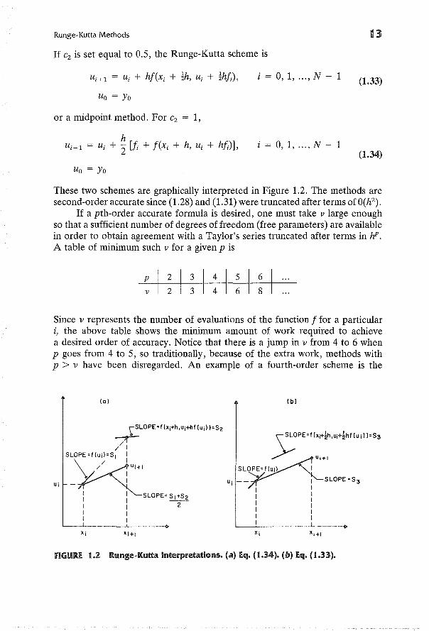
If Cz is set equal to 0.5, the Runge-Kutta scheme is
13
Ui+l = Ui + hl(xi + ~h, Ui + ~hl;),
Uo = Yo
or a midpoint method. For Cz = 1,
hU i + 1 = Ui + "2 [I; + I(xi + h, Ui + hj;)L
Uo = Yo
i = 0, 1, ... , N - 1
0,1, ... , N - 1
(1.33)
(1.34)
These two schemes are graphically interpreted in Figure 1.2. The methods aresecond-order accurate since (1.28) and (1.31) were truncated after terms of O(hZ).
If a pth-order accurate formula is desired, one must take v large enoughso that a sufficient number of degrees of freedom (free parameters) are availablein order to obtain agreement with a Taylor's series truncated after terms in hP •
A table of minimum such v for a given p is
p
v
Since v represents the number of evaluations of the function I for a particulari, the above table shows the minimum amount of work required to achievea desired order of accuracy. Notice that there is a jump in v from 4 to 6 whenp goes from 4 to 5, so traditionally, because of the extra work, methods withp > v have been disregarded. An example of a fourth-order scheme is the
(0)
+LOPE=f(Xi+h,Ui+hf (Ui»=S2
// I
SL¥<toPE=f(~~=SI: UI+I
Ui :
- I, I SLOPE= SI+S2I --
I I 2, II I
Xi Xi
(b)
SLOPE=S3
fiGURE 1.1. Ramge-I{utta interpretations. (a) (q. (1.34). (b) Eq. (1.33).
14 Initial-Value Problems for Ordinary Differential Equations
Runge-Kutta-Gill Method [41] and is:
Ui + 1 = Ui + HKI + K4) + HbK2 + dK3 )
K 2 = hf(xi + ~h, U i + ~KI)
K3 = hf(xi + ~h, Ui + aKI + bK2)
K4 = hf(xi + h, Ui + cK2 + dK3)
0- 1 2 - 0a =
2b =
2
0 0c =
2 'd = 1 + -
2
for
(1.35)
i = 0, 1, ... , N - 1 and Uo = Yo
The parameter choices in this algorithm have been made to minimize round-offerror.
Use of the explicit Runge-Kutta formulas improves the order of accuracy,but what about the stability of these methods? For example, if A is real, thesecond-order Runge-Kutta algorithm is stable for the region - 2.0 ~ Ah ~ 0,while the fourth-order Runge-Kutta-Gill method is stable for the region-2.8 ~ Ah ~ 0.
EXAMPLE 3
A thermocouple at equilibrium with ambient air at lOoC is plunged into a warmwater bath at time equal to zero. The warm water acts as an infinite heat sourceat 20°C since its mass is many times that of the thermocouple. Calculate theresponse curve of the thermocouple.
Data: Time constant of the thermocouple = 0.4 min-I.
SOLUTION
Define
Cp = thermal capacity of the thermocouple
U = heat transfer coefficient of the thermocouple
A = heat transfer area of thermocouple
t = time (min)
T, Tp' To = temperature of thermocouple, water, and ambient air
Runge-Kutta Methods
T - T6 = ---"'p-
Tp - To
C'T] = U~ = time constant of the thermocouple
tt* - 10
15
T = lOoC at t = 0
The governing differential equation is Newton's law of heating or cooling andis
dTCp di = UA(Tp -. T),
If the response curve is calculated for 0 :;;; t :;;; 10 min, then
d6dt*
The analytical solution is
-256,
6 = e-25t*,
6 = 1 at t = 0
o:;;; t* :;;; 1
Now solve the differential equation using the second-order Runge-Kutta method[Eq. (1.34)]:
Uo = 1
where
U;+l = U; + ~ [I; + f«( + h, U; + hi;)],
-25u;
i = 0, 1, ... , N - 1
f«( + h, U; + hi;) = -25(u; + hf;)
and using the Runge-Kutta-Gill method [Eq. (1.35)]:
Uo = 1
U;+l = u; + ~(Kl + K4) + ~(bK2 + dK3) , i = 0, 1, ... , N - 1
K 1 = -25hu;
K2 = -25h(u; + !K1)
K3 = -25h(u; + aK1 + bK2)
K4 = - 25h(U; + cK2 + dK3)
Table 1.3 shows the generated results. Notice that for N = 20 the secondorder Runge-Kutta method shows large discrepancies when compared with theanalytical solution. Since A = - 25, the maximum stable step-size for this methodis h = 0.08, and for N = 20, h is very close to this maximum. For the
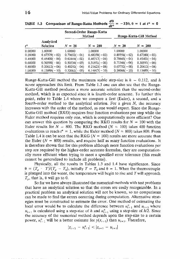
16 Initial-Value Problems for Ordinary Differential Equations
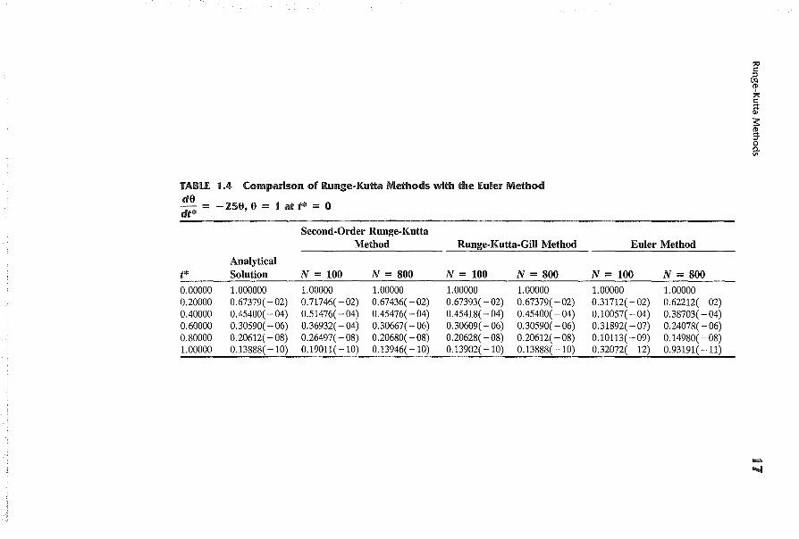
dO- 250, 0 = t at t* = 0TABLE 1.3 Comparison of Runge-Kutta Methods dt* =
Second~Order Runge-KuttaMethod Runge-Kutta-Gill Method
Analyticalt* Solution N = 20 N = 200 N = 20 N = 200
0.00000 1.00000 1.00000 1.00000 1.00000 1.000000.20000 0.67379( - 02) 0.79652(-01) 0.68350( -02) 0.89356(-02) 0.67380( -02)0040000 OA5400( - 04) 0.63444( - 02) 0046717(-04) 0.79845(-04) OA5401( - 04)0.60000 0.30590( -06) 0.50534( -03) 0.31931( - 06) 0.71346(-06) 0.30591( -06)0.80000 0.20612( -08) OA0252( -04) 0.21825( -08) 0.63752( -08) 0.20612( - 08)1.00000 0.13888( -10) 0.32061( - 05) 0.14917( -10) 0.56966( -10) 0.13889(-10)
Runge-Kutta-Gill method the maximum stable step-size is h = 0.112, and hnever approaches this limit. From Table 1.3 one can also see that the RungeKutta-Gill method produces a more accurate solution than the second-ordermethod, which is as expected since it is fourth-order accurate. To further thispoint, refer to Table 1.4 where we compare a first (Euler), a second, and afourth-order method to the analytical solution. For a given N, the accuracyincreases with the order of the method, as one would expect. Since the RungeKutta-Gill method (RKG) requires four function evaluations per step while theEuler method requires only one, which is computationally more efficient? Onecan answer this question by comparing the RKG results for N = 100 with theEuler results for N = 800. The RKG method (N = 100) takes 400 functionevaluations to reach t* = 1, while the Euler method (N = 800) takes 800. FromTable 1.4 it can be seen that the RKG (N = 100) results are more accurate thanthe Euler (N = 800) results, and require half as many function evaluations. Itis therefore shown that for this problem although more function evaluations perstep are required by the higher-order accurate formulas, they are computationally more efficient when trying to meet a specified error tolerance (this resultcannot be generalized to include all problems).
Physically, all the results in Tables 1.3 and 1.4 have significance. Sincee = (Tp - T)/(Tp - To), initially T = To and e = 1. When the thermocoupleis plunged into the water, the temperature will begin to rise and Twill approachTp , that is, e will go to O.
So far we have always illustrated the numerical methods with test problemsthat have an analytical solution so that the errors are easily recognizable. In apractical problem an analytical solution will not be known, so no comparisonscan be made to find the errors occurring during computation. Alternative strategies must be constructed to estimate the error. One method of estimating thelocal error would be to calculate the difference between u,!+ 1 and Ui + 1 whereU i + 1 is calculated using a step-size of hand U'!+l using a step-size of h/2. Sincethe accuracy of the numerical method depends upon the step-size to a certainpower, U'!+l will be a better estimate for Y(Xi +l) than Ui + 1• Therefore,
TABU 1.4 Comparison of Runge·Kutta Methods with the Euler MethoddO- = -250, 0 = 1 at t* = 0dt*
Second·Order Runge.KuttaMethod Runge-Kutta-Gill Method Euler Method
Analyticalt* Solution N = 100 N = 800 N = 100 N = 800 N = 100 N = 800
0.00000 1.000000 1.00000 1.00000 1.00000 1.00000 1.00000 1.000000.20000 0.67379( -02) 0.71746( -02) 0.67436( -02) 0.67393(-02) 0.67379( -02) 0.31712( -02) 0.62212( - 02)0.40000 0.45400(-04) 0.51476(-04) 0.45476( - 04) 0.45418(-04) 0.45400( - 04) 0.10057(-04) 0.38703(-04)0.60000 0.30590( -06) 0.36932( - 04) 0.30667( - 06) 0.30609( -06) 0.30590( -06) 0.31892( -07) 0.24078( -06)0.80000 0.20612( - 08) 0.26497( -08) 0.20680( - 08) 0.20628( - 08) 0.20612( -08) 0.10113(-09) 0.14980(-08)1.00000 0.13888( -10) 0.19011( -10) 0.13946( -10) 0.13902( -10) 0.13888( -10) 0.32072( -12) 0.93191( -11)
e'~(J)
~s=$:(J)
9'o0..VI
-"'-I
18
and
Initial-Value Problems for Ordinary Differential Equations
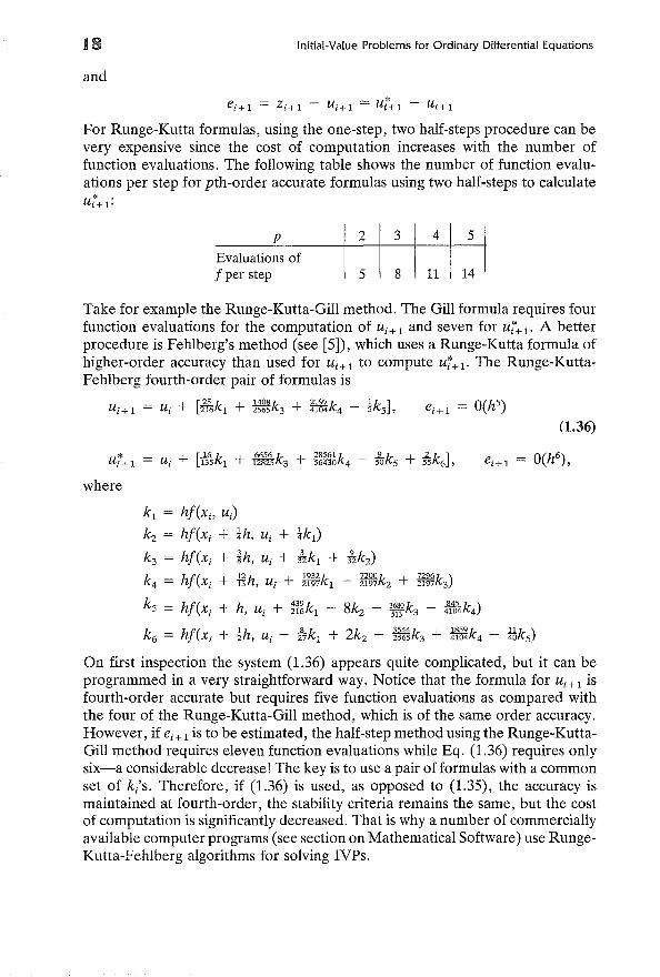
For Runge-Kutta formulas, using the one-step, two half-steps procedure can bevery expensive since the cost of computation increases with the number offunction evaluations. The following table shows the number of function evaluations per step for pth-order accurate formulas using two half-steps to calculateU7+1:
p
Evaluations offper step
2
5
3
8
4 5
11 14
Take for example the Runge-Kutta-Gill method. The Gill formula requires fourfunction evaluations for the computation of Ui+1 and seven for U7+1' A betterprocedure is Fehlberg's method (see [5]), which uses a Runge-Kutta formula ofhigher-order accuracy than used for Ui+1 to compute U7+1' The Runge-KuttaFehlberg fourth-order pair of formulas is
[25 k 1408k 2197k 1k ]Ui + 1 = Ui + 216 1 + 2565 3 + 4104 4 - :5 5 ,
[16 k 6656 k 28561 k 9 k + 2 k ]
U i + 135 1 + 12825 3 + 56430 4 - 55 5 55 6 ,
where
k1 = hf(xi, uJk2 = hf(xi + ~h, Ui + ~kl)
k3 = hf(Xi + ih, ui + iik1 + !zk2)
k4 = hf(xi + Hh, Ui + ~~~~kl - iig~k2 + ii~~k3)
k - hf( + h + mk 8k + 3680k - M2..k)5 - Xi ,Ui 216 1 - 2 ill 3 4104 4
On first inspection the system (1.36) appears quite complicated, but it can beprogrammed in a very straightforward way. Notice that the formula for U i + 1 isfourth-order accurate but requires five function evaluations as compared withthe four of the Runge-Kutta-Gill method, which is of the same order accuracy.However, if ei+l is to be estimated, the half-step method using the Runge-KuttaGill method requires eleven function evaluations while Eq. (1.36) requires onlysix-a considerable decrease! The key is to use a pair of formulas with a commonset of k/s. Therefore, if (1.36) is used, as opposed to (1.35), the accuracy ismaintained at fourth-order, the stability criteria remains the same, but the costof computation is significantly decreased. That is why a number of commerciallyavailable computer programs (see section on Mathematical Software) use RungeKutta-Fehlberg algorithms for solving IVPs.
Implicit Methods 19
(1.37)
In this section we have presented methods that increase the order of accuracy, but their stability limitations remain severe. In the next section we discussmethods that have improved stability criteria.
IMPLICIT METHODS
If we once again consider Eq. (1.7) and expand y(x) about the point Xi + 1 usingTaylor's theorem with remainder:
Y(Xi) = Y(Xi+1) - hy'(Xi+1) + ~~ Y"(~i)'
Substitution of (1.7) into (1.37) gives
y(xi) = Y(Xi+1) - hf(xi+1' Y(Xi+1))
h2 _ _
+ 2! t: (~, y(~)), (1.38)
A numerical procedure of (1.7) can be obtained from (1.38) by truncating afterthe second term:
Uo = Yo
i = 0, 1, ... , N - 1, (1.39)
(1.40)
Equation (1.39) is called the implicit Euler method because the function f isevaluated at the right-hand side of the subinterval. Since the value of U i + 1 isunknown, (1.39) is nonlinear iffis nonlinear. In this case, one can use a Newtoniteration (see Appendix B). This takes the form
[s+1] _ h[fl afl ([S+1] Is] )]Ui+1 - [s]. + ay [s] Ui+1 - Ui+1 + Uiu 1+1 U l +l
or after rearrangement
( 1 - h af) I ([S+1] - [s]) - hil Is]ay u['] Ui+1 Ui+1 - ['I + Ui - Ui+11+1 U 1+ 1
where U~11 is the sth iterate of Ui+1. Iterate on (1.41) until
IU~~";.1] - U!111 ~ TOL
(1.41)
(1.42)
where TOL is a specified absolute error tolerance.One might ask what has been gained by the implicit nature of (1.39) since
it requires more work than, say, the Euler method for solution. If we apply theimplicit Euler scheme to (1.17) (X. real),
20
or
Initial-Value Problems for Ordinary Differential E.quations
(1.43)_ ( 1 ) _ ( 1 );+1U; + 1 - 1 _ h'A U; - 1 _ h'A Yo
If 'A < 0, then (1.39) is stable for all h > °or it is unconditionally stable, andnever oscillates.
The implicit nature of the method has stabilized the algorithm, but unfortunately the scheme is only first-order accurate. To obtain a higher order ofaccuracy, combine (1.38) and (1.10) to give
i = 0, 1, ... , N - 1,
2[Y(Xi+1) - y(x;)] = h[/;+1 + /;] + O(h3)
The algorithm associated with (1.44) is
hU;+1 = U; + 2 [/;+1 + /;],
(1.44)
(1.45)
Uo = Yo
which is commonly called the trapezoidal rule. Equation (1.45) is second-orderaccurate, and the stability of the scheme can be examined by applying the methodto (1.17), giving ('A real)
(1 + ¥)(1 _~h)
;+1
Yo (1.46)
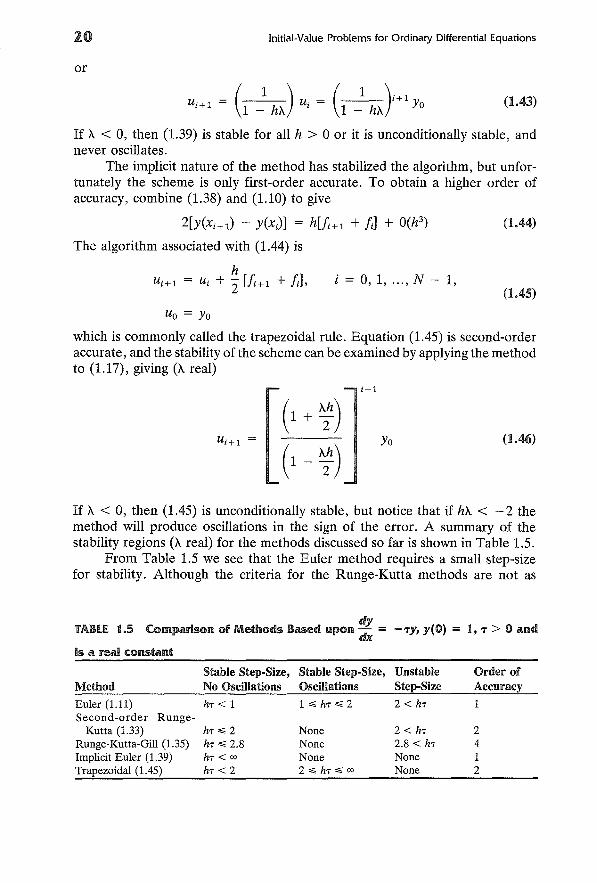
If 'A < 0, then (1.45) is unconditionally stable, but notice that if h'A < - 2 themethod will produce oscillations in the sign of the error. A summary of thestability regions ('A real) for the methods discussed so far is shown in Table 1.5.
From Table 1.5 we see that the Euler method requires a small step-sizefor stability. Although the criteria for the Runge-Kutta methods are not as
dyTABLE 1.5 Comparison of Methods Based upon dx = -TY, y(O) = t, T > 0 and
is a real constant
Stable Step-Size, Stabie Step-Size, Unstable Order ofMethod No Oscillations Oscillations Step-Size Accuracy
Euler (1.11) hT < 1 10;;; hT 0;;; 2 2 < hT 1Second-order Runge-
Kutta (1.33) hT 0;;; 2 None 2 < hT 2Runge-Kutta-Gill (1.35) hT 0;;; 2.8 None 2.8 < hT 4Implicit Euler (1.39) hT < 00 None None 1Trapezoidal (1.45) hT < 2 2 0;;; hT 0;;; 00 None 2
Extrapolation 21
(1.47)
stringent as for the Euler method, stable step-sizes for these schemes are alsoquite small. The trapezoidal rule requires a small step-size to avoid oscillationsbut is stable for any step-size, while the implicit Euler method is always stable.The previous two algorithms require more arithmetic operations than the Euleror Runge-Kutta methods when f is nonlinear due to the Newton iteration, butare typically used for solution of certain types of problems (see section onstiffness) .
In Table 1.5 we once again see the dilemma of stability versus accuracy.In the following section we outline one technique for increasing the accuracywhen using any method.
EXTRAPOLATION
Suppose we solve a problem with a step-size of h giving the solution Ui at Xi'and also with a step-size h/2 giving the solution Wi at Xi' If an Euler method isused to obtain Ui and Wi' then the error is proportional to the step-size (firstorder accurate). If Y(x i ) is the exact solution at X;, then
Ui = Y(xi) + <l>h
hWi = Y(Xi) + <1>2"
where <I> is a constant. Eliminating <I> from (1.47) gives
Y(xi) = 2Wi - Ui (1.48)
If the error formulas (1.47) are exact, then this procedure gives the exact solution.Since the formulas (1.47) usually only apply as h ~ 0, then (1.48) is only anapproximation, but it is expected to be a more accurate estimate than either Wior Ui' The same procedure can be used for higher-order methods. For the trapezoidal rule
EXAMPLE 4
Ui = Y(Xi) + <l>h2
Wi = Y(Xi) + <I> (~) 2
4w· - UiY(Xi) = 1
3
(1.49)
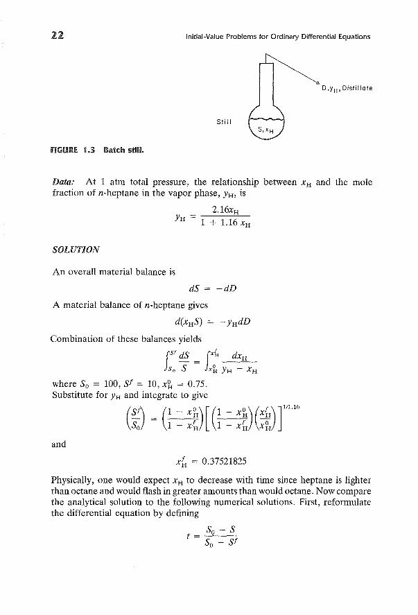
The batch still shown in Figure 1.3 initially contains 25 moles of n-octane and75 moles of n-heptane. If the still is operated at a constant pressure of 1 atmosphere (atm) , compute the final mole fraction of n-heptane, x{.p if the remaining solution in the still, Sf, totals 10 moles.
22 Initial-Value Problems for Ordinary Differential Equations
fiGURE 1.3 Batch still.
Still
D 'YH' Distillate
Data: At 1 atm total pressure, the relationship between XH and the molefraction of n-heptane in the vapor phase, YH, is
2. 16xHYH = 1 + 1.16 XH
SOLUTION
An overall material balance is
dS = -dD
A material balance of n-heptane gives
d(xHS)
Combination of these balances yields
rSf dS rx{, dXH
Js o S = Jx'i, YH - XH
where So = 100, Sf = 10, x~ = 0.75.Substitute for YH and integrate to give
(Sf) (1 - X~)[(l _ X~)(X~)]1/1.16SO 1 - x~ 1 - x~ x~
and
X~ = 0.37521825
Physically, one would expect XH to decrease with time since heptane is lighterthan octane and would flash in greater amounts than would octane. Now comparethe analytical solution to the following numerical solutions. First, reformulatethe differential equation by defining
So - St=---"---
So - Sf
Extrapolation
so that
Thus:
dXH-=dt
O~t~l
1.16 (Sf - So) xH(l - XH)
(So(l - t) + Sft) (1 + 1. 16xH) ,at t = 0
23
If an Euler method is used, the results are shown in Table 1.6. From a practicalstandpoint, all the values in Table 1.6 would probably be sufficiently accuratefor design purposes, but we provide the large number of significant figures toillustrate the extrapolation method. A simple Euler method is first-order accurate, and so the truncation error should be proportional to h(1/N). This isshown in Table 1.6. Also notice that the error in the extrapolated Euler methoddecreases faster than that in the Euler method with increasing N. The truncationerror of the extrapolation is approximately the square of the error in the basicmethod. In this example one can see that improved accuracy with less computation is achieved by extrapolation. Unfortunately, the extrapolation is successfulonly if the step-size is small enough for the truncation error formula to bereasonably accurate. Some nonlinear problems require extremely small stepsizes and can be computationally unreasonable.
Extrapolation is one method of increasing the accuracy, but it does notchange the stability of a method. There are commercial packages that employextrapolation (see section on Mathematical Software), but they are usually basedupon Runge-Kutta methods instead of the Euler or trapezoidal rule as outlined
TABU t.6 Errors in the Euler Method andthe Extrapolated Euler Method for Exam·pie 4
Number ofSteps
AbsoluteTotal Number Valueof Steps of the Error
Euler Method
50100200400800
1,600
50100200400800
1,600
0.013730.006750.003350.001660.000830.00041
Extrapolated Euler Method
50-100 150100-200 300200-400 600400-800 1,200800-1600 2,400
0.0002200.0000560.0000130.0000030.000001
24 Initial-Value Problems for Ordinary Differential Equations
(1.50)
above. In the following section we describe techniques currently being used insoftware packages for which stability, accuracy, and computational efficiencyhave been addressed in detail (see, for example, [5]).
MULTISTEP METHODS
Multistep methods make use of information about the solution and its derivativeat more than one point in order to extrapolate to the next point. One specificclass of multistep methods is based on the principle of numerical integration. Ifthe differential equation y' = f(x, y) is integrated from Xi to Xi+l' we obtain
J:"+1 y' dx = J:"+1 f(x, y(x» dx
or
Y(Xi+l) = y(x;) + {'+1 f(x, y(x» dx
To carry out the integration in (1.50), approximate f(x, y(x» by a polynomialthat interpolates f(x, y(x» at k points, Xi' Xi-l, ... , Xi-k+l. If the Newtonbackward formula of degree k-l is used to interpolate f(x, y(x», then theAdams-Bashforth formulas [1] are generated and are of the form
where
k
Ui+l = Ui + h 2,bjU!-j+lj=l
(1.51)
U; = f(xj' Uj)
This is called a k-step formula because it uses information from the previous ksteps. Note that the Euler formula is a one-step formula (k = 1) with b l = 1.Alternatively, if one begins with (1.51), the coefficients bj can be chosen byassuming that the past values of U are exact and equating like powers of h inthe expansion of (1.51) and of the local solution Zi+1 about Xi. In the case of athree-step formula
Substituting values of Z into this and expanding about Xi gives
Zi+l = Zi + hz;[b1 + b2 + b3] - h2z7[b2 + 2b3] + ~~ zt[b2 + 4b3] + ...
whereh2
Z,'-l = z,~ - hz'! + - Z~II +I 2!'
4h2
Z,'-2 = z,' - 2hz~' + - Z~II +, 2!'
Multistep Methods
The Taylor's series expansion of Zi+ 1 is
hZ h3
Z,"+l = Z," + hZ,~ + -z" + -ZIII +2! l 3! l
and upon equating like power of h, we have
bl + bz + b3 = 1
25
1-2:
The solution of this set of linear equations is bl = ~, bz = -~, and b3
Therefore, the three-step Adams-Bashforth formula is
Ui + l = Ui + :2 [23ul - 16ul_ l + 5u;_z]
2.12·
(1.52)
with an error ei + 1 = O(h4) [generally ei + l = O(hk + l ) for any value of k; forexample, in (1.52) k = 3].
A difficulty with multistep methods is that they are not self-starting. In(1.52) values for Ui, u;, U;-l, and u;-z are needed to compute Ui+l' The traditional technique for computing starting values has been to use Runge-Kuttaformulas of the same accuracy since they only require Uo to get started. Analternative procedure, which turns out to be more efficient, is to use a sequenceof s-step formulas with s = 1, 2, . . . , k [6]. The computation is started withthe one-step formulas in order to provide starting values for the two-step formulaand so on. Also, the problem of getting started arises whenever the step-size his changed. This problem is overcome by using a k-step formula whose coefficients (the b/s) depend upon the past step-sizes (hs = Xs - Xs-l' S = i, i - 1,... ,i - k + 1) (see [6]). This kind of procedure is currently used in commercialmultistep routines.
The previous multistep methods can be derived using polynomials thatinterpolated at the point Xi and at points backward from Xi' These are sometimesknown as formulas of explicit type. Formulas of implicit type can also be derivedby basing the interpolating polynomial on the point Xi+l' as well as on Xi andpoints backward from Xi' The simplest formula of this type is obtained if theintegral is approximated by the trapezoidal formula. This leads to
which is Eq. (1.45). Iffis nonlinear, U i + 1 cannot be solved for directly. However,we can attempt to obtain Ui + 1 by means of iteration. Predict a first approximationU)~l to Ui+l by using the Euler method
[0] _ + h,-rU i + 1 - Ui :Ii (1.53)
26 Initial-Value Problems for Ordinary Differential Equations
(1.54)
Then compute a corrected value with the trapezoidal formula
ul~~l] = Ui + ~ Lt; + !(ull1)], s = 0, 1, ...
For most problems occurring in practice, convergence generally occurs withinone or two iterations. Equations (1.53) and (1.54) used as outlined above definethe simplest predictor-corrector method.
Predictor-corrector methods of higher-order accuracy can be obtained byusing the multistep formulas such as (1.52) to predict and by using correctorformulas of type
k
Ui + 1 = Ui + h L bj U;_j+lj=O
(1.55)
Notice that j now sums from zero to k. This class of corrector formulas is calledthe Adams-Moulton correctors. The b/s of the above equation can be found ina manner similar to those in (1.52). In the case of k = 2,
(1.56)
with a local truncation error of 0(h4). A similar procedure to that outlined forthe use of (1.53) and (1.54) is constructed using (1.52) as the predictor and(1.56) as the corrector. The combination (1.52), (1.56) is called the AdamsMoulton predictor-corrector pair of formulas.
Notice that the error in each of the formulas (1.52) and (1.56) is 0(h4).
Therefore, if ei + 1 is to be estimated, the difference
Ui+l from (1.56), Ui +l from (1.52)
would be a poor approximation. More precise expressions for the errors in theseformulas are [5]
for (1.52)
for (1.56)
where Xi - 2 < ~ and ~* < X i + 1• Assume that ~* = ~ (this would be a goodapproximation for small h), then subtract the two expressions.
ei+l - ei + 1 = Ui+l - Ui + 1 = - fzh4y""(~)
Solving for h4y""(~) and substituting into the expression ei+l gives
1*1_.1.1* 1ei + 1 - 10 Ui + 1 - Ui+l
Since we had to make a simplifying assumption to obtain this result, it is betterto use a more conservative coefficient, say /;. Hence,
I * 1-.1 I * Iei + 1 - 8 Ui + 1 - Ui + 1 (1.57)
Multistep Methods 27
Note that this is an error estimate for the more accurate value so that Ui+1 canbe used as the numerical solution rather than Ui +1' This type of analysis is notused in the case of Runge-Kutta formulas because the error expressions are verycomplicated and difficult to manipulate in the above fashion.
Since the Adams-Bashforth method [Eq. (1.51)] is explicit, it possessespoor stability properties. The region of stability for the implicit Adams-Moultonmethod [Eq. (1.55)] is larger by approximately a factor of 10 than the explicitAdams-Bashforth method, although in both cases the region of stability decreases as k increases (see p. 130 of [4]). For the Adams-Moulton predictorcorrector pair, the exact regions of stability are not well defined, but the stabilitylimitations are less severe than for explicit methods and depend upon the numberof corrector iterations [4].
The multistep integration formulas listed above can be represented by thegeneralized equation:
k j k2
Ui + 1 = 2: ai+1,j Ui -j+1 + h i+ 1 2: b i + 1,j u:- j + 1j=l j=O
(1.58)
which allows for variable step-size through h i + 1, a i+ 1,j, and b i + 1,j' For example,if k1 = 1, a i + 1,1 = 1 for all i, b i + 1,j = bi,j for all i, and kz = q - 1, then aqth-order implicit formula is obtained. Further, if bi + 1,0 = 0, then an explicit formulais generated. Computationally these methods are very efficient. If an explicitformula is used, only a single function evaluation is needed per step. Becauseof their poor stability properties, explicit multistep methods are rarely used inpractice. The use of predictor-corrector formulas does not necessitate the solution of nonlinear equations and requires S + 1 (S is the number of correctoriterations) function evaluations per step in x. Since S is usually small, fewerfunction evaluations are required than from an equivalent order of accuracyRunge-Kutta method and better stability properties are achieved. If a problemrequires a large stability region (see section of stiffness), then implicit backwardformulas must be used. If (1.58) represents an implicit backward formula, thenit is given by
k j
Ui + 1 2: a i + 1,j Ui - j + 1 + h i + 1 b i + 1,0 u:+ 1j=l
orUi + 1 = bi+1,0 hi+1 f(Ui+1) + <Pi (1.59)
where <Pi is the grouping of all known information. If a Newton iteration isperformed on (1.59), then
[1 - bi+1,0 h i + 1 :; ui1J [Ui~~l] - ui11]
= b i + 1,0 h i + 1 fl u[s] + <Pi - ui11'i+1
s = 0,1, ... (1.60)
28 Initial-Value Problems for Ordinary Differential Equations
Therefore, the derivative aflay must be calculated and the function f evaluatedat each iteration. One must "pay" in computation time for the increased stability.The order of accuracy of implicit backward formulas is determined by the valueof k 1• As k1 is increased, higher accuracy is achieved, but at the expense ofdecreased stability (see Chapter 11 of [4]).
Multistep methods are frequently used in commercial routines because oftheir combined accuracy, stability, and computational efficiency properties (seesection on Mathematical Software). Other high-order methods for handlingproblems that require large regions of stability are discussed in the followingsection.
HIGH-ORDER METHODS BASED ON KNOWLEDGE Of {)ff{Jy
A variety of methods that make use of aflay has been proposed to solve problemsthat require large stability regions. Rosenbrock [7] proposed an extension of theexplicit Runge-Kutta process that involved the use of aflay. Briefly, if one allowsthe summation in (1.25) to go from 1 to j, i.e., an implicit Runge-Kutta method,then,
(1.61)
If kj is expanded,
(
j-1 )kj = hf U i + 2: a'zkzZ= 1 ]
(1.62)
and rearranged to give
[af ( j -1 _ )] _ ( j -1 _ )
1 - hajj - Ui + 2: a'lkZ kj = hf Ui + 2: a·zkzay Z=1 ] Z=1 ](1.63)
the method is called a semi-implicit Runge-Kutta method. In the function f, itis assumed that the independent variable x does not appear explicitly, i.e., it isautonomous. Equation (1.63) is used with
v
Ui + 1 = Ui + 2: wjkjj=1
(1.64)
to specify the method. Notice that if the bracketed term in (1.63) is replacedby 1, then (1.63) is an explicit Runge-Kutta formula. Calahan [8], Allen [9],and Caillaud and Padmanabhan [10] have developed these methods into algorithms and have shown that they are unconditionally stable with no oscillationsin the solution. Stabilization of these algorithms is due to the bracketed term in(1.63). We will return to this semi-implicit method in the section MathematicalSoftware.
Other methods that are high-order, are stable, and do not oscillate are the
Stiffness 29
second- and third-order semi-implicit methods of Norsett [11], more recentlythe diagonally implicit methods of Alexander [12], and those of Bui and Bui[13] and Burka [14].
STIffNESS
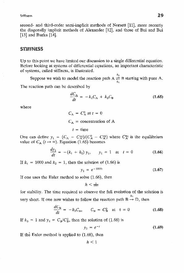
Up to this point we have limited our discussion to a single differential equation.Before looking at systems of differential equations, an important characteristicof systems, called stiffness, is illustrated.
k 1
Suppose we wish to model the reaction path A :;::::=: B starting with pure A.k2
The reaction path can be described by
dCA--;It = - k1CA + kZCB (1.65)
where
CA = C1 at t = 0
CA = concentration of A
t = time
One can define Y1 = (CA - C~)I(C~ - C~) where C~ is the equilibriumvalue of CA (t -i> 00). Equation (1.65) becomes
dYl =dt -(k1 + kz) Yl' Yl = 1 at t = 0 (1.66)
If k 1 = 1000 and kz = 1, then the solution of (1.66) is
(1.67)
If one uses the Euler method to solve (1.66), then
h < llOlfor stability. The time required to observe the full evolution of the solution is
k3
very short. If one now wishes to follow the reaction path B -i> D, then
dCB 0----;[( = -k3CB , CB = CB at t = 0 (1.68)
If k3 = 1 and Yz = CB/C~, then the solution of (1.68) is
Yz = e- t
If the Euler method is applied to (1.68), then
h<1
(1.69)
30 Initial-Value Problems for Ordinary Differential Equations
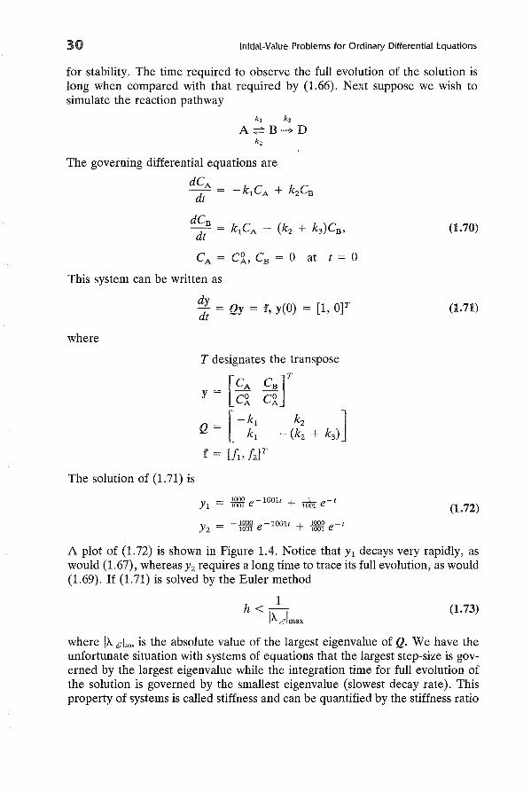
for stability. The time required to observe the full evolution of the solution islong when compared with that required by (1.66). Next suppose we wish tosimulate the reaction pathway
(1.71)
(1.70)
[l,OyQy = f, yeO)
The governing differential equations are
dCA"dt = -k1CA + k2CB
dCB _ k C - (k k )Cdt - 1 A 2 + 3 B'
CA = Cl, CB = 0 at t = 0
This system can be written as
dydt
where
The solution of (1.71) is
(1.72)
A plot of (1.72) is shown in Figure 1.4. Notice that Yl decays very rapidly, aswould (1.67), whereas Y2 requires a long time to trace its full evolution, as would(1.69). If (1.71) is solved by the Euler method
1h < - (1.73)
IAG'lmax
where III. glma. is the absolute value of the largest eigenvalue of Q. We have theunfortunate situation with systems of equations that the largest step-size is governed by the largest eigenvalue while the integration time for full evolution ofthe solution is governed by the smallest eigenvalue (slowest decay rate). Thisproperty of systems is called stiffness and can be quantified by the stiffness ratio
Stiffness
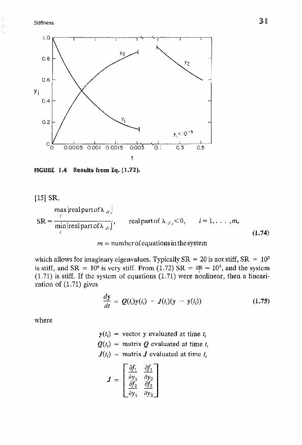
I.0 ,----,---.,.-----r--,..-'Ir--'V-,------,---,---,
31
0.8
0.6
Yj0.4
0.2
0.0005 0.001 0.0015 0.003 0.1 0.3 0.5
fiGURE 1.4 Results from Eq. (1.72).
[15] SR,
maxlrealpartofA 6',1i
SR = . I 1 f I'mm rea parto A6',;
realpartof A6',<0, i= 1, ... ,m,
(1.74)
m = numberofequationsinthesystem
which allows for imaginary eigenvalues. Typically SR = 20 is not stiff, SR = 103
is stiff, and SR = 106 is very stiff. From (1.72) SR = 10101 = 103
, and the system(1.71) is stiff. If the system of equations (1.71) were nonlinear, then a linearization of (1.71) gives
where
dydt = Q(t;)y(t;) + J(t;)(y - yeti))
yeti) = vector y evaluated at time t;
Q(t;) = matrix Q evaluated at time t;
J(t;) = matrix J evaluated at time t;
(1.75)
32 Initial-Value Problems for Ordinary Differential Equations
The matrix J is called the Jacobian matrix, and in general is
all all allaY1' ayz' ... , aYm
J=aim aim aimay/ ayz' ... , aYm
For nonlinear problems the stiffness is based upon the eigenvalues of J and thusapplies only to a specific time, and it may change with time. This characteristicof systems makes a problem both interesting and difficult. We need to classifythe stiffness of a given problem in order to apply techniques that "perform"well for that given magnitude of stiffness. Generally, implicit methods "outperform" explicit methods on stiff problems because of their less rigid stabilitycriterion. Explicit methods are best suited for nonstiff equations.
SYSnMS Of DiffERENTIAL EQUATIONS
A straightforward extension of (1.11) to a system of equations is
i = 0, 1, ... , N - 1 (1.76)
Uo = Yo
Likewise, the implicit Euler becomes
"0 = Yo
while the trapezoid rule gives
h"i+1 = "i + '2 [f(xi, "i+1) + f(xi, "i)],
Uo = Yo
i = 0, 1, ... , N - 1
i = 0, 1, ... , N - 1
(1.77)
(1.78)
For a system of equations the Runge-Kutta-Fehlberg method is
* + [16 k 6656 k 28561 k 9 k 2 k ]"i + 1 = "i 135 1 + 12825 3 + 56430 4 - 55 5 + 55 6
where
k . = [k{l} k{Z} k~m}]TZ l , I'··" I
(1.79)
Systems of Differential E.quations
and, for example,
k {]} - h.f ( {I} {2} {m})1 - 1j Xi' Ui ,Ui , ... ,Ui , j = 1, ... ,m
33
<Pji = u}J1 + ~k¥1
k¥1 = h/i(xi + ~h, <P1i' <P2;, ... , <Pmi), j = 1, ... ,m
(1.80)
The Adams-Moulton predictor-corrector formulas for a system of equations are
U i + 1 = Ui + :2 [23uI - 16uI_1 + 5uI-z]
*- h[5' 8' ']Ui+ 1 - U i + 12 Ui+1 + U i - Ui-1
An algorithm using the higher-order method of Caillaud and Padmanabhan[10] was formulated by Michelsen [16] by choosing the parameters in (1.63) sothat the same factor multiplies each k;, thus minimizing the work involved inmatrix inversion. The final scheme is
i = 0, 1, ... , N - 1
Uo = Yo
_ [ af]-lk 1 = h I - hal ay (Ui) feu;)
_ [ af] -1 _k2 = h I - hal ay (Ui) f(u i + b2k1)
_ [ af] -1 _ _k3 = h I - hal ay (Ui) (b31k 1 + b32k2)
where I is the identity matrix,
a1 = 0.43586659
b2 = 0.75
-1b31 = -6 (8at - 2a1 + 1)
a1
2b32 = -9 (6at - 6a1 + 1)
a1
(1.81)
34 Initial-Value Problems for OrdinalY Differential Equations
(1.82)
As previously stated, the independent variable x must not explicitly appear inf. If x does explicitly appear in f, then one must reformulate the system ofequations by introducing a new integration variable, t, and let
dx- = 1dt
be the (m + 1) equation in the system.
EXAMPLE 5
Referring to Example 1, if we now consider the reactor to be adiabatic insteadof isothermal, then an energy balance must accompany the material balance.Formulate the system of governing differential equations and evaluate the stiffness. Write down the Euler and the Runge-Kutta-Fehlberg methods for thisproblem.
DataCp = 12.17 X 10⁴ J/(kmole'°C)
- b.Hr = 2.09 x 10⁸ J/kmole
SOLUTION
Let T* = TlTo, TO = 423 K (150°C). For the "short" reactor, .
dy [3.21]dx = -0.1744 exp T* y (material balance)
dT* [3.21]dx = 0.06984 exp T* y (energy balance)
y = 1, T* = 1 at x = 0
First, check to see if stiffness is a problem. To do this the transport equationscan be linearized and the Jacobian matrix formed.
J =
(3.21)-0.1744 exp T*
(3.21)0.06984 exp T*
0.56 (3.21)(T*)Z exp T* y
- 0.224 (3.21)(T*)Z exp T* y
At the inlet T* = 1 and y = 1, and the eigenvalues of J are approximately(6.3, -7.6). Since T* should increase as y decreases, for example, if T* = 1.12and y = 0.5, then the eigenvalues of J are approximately (3.0, -4.9). Fromthe stiffness ratio, one can see that this problem is not stiff.
Systems of Differential Equations
Euler:
U{1} = U{1} - 01744 exp [3.21] U{1} hz+1 I' U{2} zz
U{2} = U{2} + 006984 exp [3.21] U{1} hz+ 1 z· U{2} z
z
ub1} = 1
U{2} = 1o
Runge-Kutta-Fehlberg:
ui21 = ui1}+ [C1·ki1}+ C2'k~1} + C3·kr} + C4'k~1}]
U{2} = U{2} + [C1'k{2} + C2·k{2} + C3·k{2} + C4·k{2}]z+l z 1 3 4 5
U{1}* = u{l} + [C5·k{l} + C6·k{1} + C7·k{1} + C8·k{1} + C9·k{1}]z+1 I 1 3 4 5 6
U{2}* = U{2} + [C5'k{2} + C6·k{2} + C7·k{2} + C8·k{2} + C9·k{2}]z+1 z 1 3 4 5 6
35
C1 = ii6,
C2 = i~~~,
C3 = ~i~~,
C5 = 1~~
C6 = 1~6i;5
C7 = ~~~~6
C4 = -!, C8 = 9-so
C9 = is
Define
[3.21]F1(A, B) = -0.1744 exp 13 A
[3.21]F2(A, B) = 0.06984 exp 13 A
then
k{l} = hF1(u{l} U{2})1 l , l
ki2} = hF2(ui1}, ui2})
k~1} = hF1(ui1} + ~ki1}, ui2} + ~ki2})
k~2} = hF2(ui1} + ~kil}, ui2} + ~ki2})
36
STEP-SIZE STRATEGIES
Initial-Value Problems for Ordinary Differential E.quations
(1.84)
(1.86)
(1.85)
Thus far we have only concerned ourselves with constant step-sizes. Variablestep-sizes can be very useful for (1) controlling the local truncation error and(2) improving efficiency during solution of a stiff problem. This is done in allof the commercial programs, so we will discuss each of these points in furtherdetail.
Gear [4] estimates the local truncation error and compares it with a desirederror, TOL. If the local truncation error has been achieved using a step-size hI,
e = <!>h~ + 1 (1.83)
Since we wish the error to equal TOL,
TOL = <!>h~+1
Combination of (1.83) and (1.84) gives
[ ]
1/(P+l)
h - h TOL2 - 1 e
Equation (1.83) is method-dependent, so we will illustrate the procedure witha specific method. If we solve a given problem using the Euler method,
Ui+l = Ui + hd(uJ
and the implicit Euler,
(1.87)
and subtract (1.86) and (1.87) from (1.10) and (1.38), respectively (assumingUi = Yi), then
Ui+l - Y(Xi+1) = - ~hi Ii + O(hI)
Wi+l - Y(Xi+l) = ~hf Ii + O(hI)
The truncation error can now be estimated by
The process proceeds as follows:
(1.88)
(1.89)
(1.90)
1.
2.3.
4.
Equations (1.86) and (1.87) are used to obtain Ui+l and Wi+l.
The truncation error is obtained from (1.89).
If the truncation error is less than TOL, the step is accepted; if not, thestep is repeated.
In either case of step(3), the next step-size is calculated according to
(TOL) 1/2
h2 = hI -ei + 1
Mathematical Software 37
To avoid small errors, one can use an h2 that is a certain percentage smallerthan calculated by (1.90).
Michelsen [16] solved (1.81) with a step-size of h and then again withh/2. The semi-implicit algorithm is third-order accurate, so it may be written as
(1.91)
(1.92)
where gh4 is the dominant, but still unknown, error term. If Ui+1 denotes thenumerical solution for a step-size of h, and OOi+ 1 for a step-size of h/2, then,
Ui+1 = Y(Xi+1) + gh4 + 0(h5)
OOi+1 = Y(Xi+1) + 2g (i) 4 + 0(h5)
where the 2g in (1.92) accounts for error accumulation in each of the twointegration steps. Subtraction of the two equations (1.92) from one another gives
(1.93)
Provided ei + 1 is sufficiently small, the result is accepted. The criterion for stepsize acceptance is
where
j = 1,2, ... ,m (1.94)
e{j} = local truncation error for the j component
If this criterion is not satisfied, the step-size is halved and the integration repeated. When integrating stiff problems, this procedure leads to small stepswhenever the solution changes rapidly, often times at the start of the integration.As soon as the stiff component has faded away, one observes that the magnitudeof e decreases rapidly and it becomes desirable to increase the step-size. Aftera successful step with hi' the step-size hi+1 is adjusted by
. [{ I e{j} I} -1/4 ]hi+1 = hi mIll 4 max TOL{j} ,3, j = 1, 2, ... , m (1.95)
For more explanation of (1.95) see [17]. A good discussion of computer algorithms for adjusting the step-size is presented by Johnston [5] and by Krogh[18].
We are now ready to discuss commercial packages that incorporate a varietyof techniques for solving systems of IVPs.
MATHEMATICAL SOfTWARE
Most computer installations have preprogrammed computer packages, i.e., software, available in their libraries in the form of subroutines so that they can beaccessed by the user's main program. A subroutine for solving IVPs will bedesigned to compute a numerical solution over [xa, XN] and return the value UN
38 Initial-Value Problems for Ordinary Differential Equations
given xo, XN' and Uo' A typical calling sequence could be
CAll DRIVE (FUNC, X, XEND, U, TOl),
where
FUNC = a user-written subroutine for evaluating f(x, y)
X = Xo
XEND= XN
U = on input contains Uo and on output contains UN
TOL = an error tolerance
This is a very simplified call sequence, and more elaborate ones are actuallyused in commercial routines.
The subroutine DRIVE must contain algorithms that:
1. Implement the numerical integration
2. Adapt the step-size
3. Calculate the local error so as to implement item 2 such that the globalerror does not surpass TaL
4. Interpolate results to XEND (since h is adaptively modified, it is doubtfulthat XEND will be reached exactly)
Thus, the creation of a software package, from now on called a code, is anontrivial problem. Once the code is completed, it must contain sufficient documentation. Several aspects of documentation are significant (from [24]):
1. Comments in the code identifying arguments and providing general instructions to the user (this is valuable because often the code is separated fromthe other documentation)
2. A document with examples showing how to use the code and illustratinguser-oriented aspects of the code
3. Substantial examples of the performance of the code over a wide range ofproblems
4. Examples showing misuse, subtle and otherwise, of the code and examplesof failure of the code in some cases.
Most computer facilities have at least one of the following mathematicallibraries:
IMSl [19]NAG [20]
HARWEll [21]
Mathematical Software 39
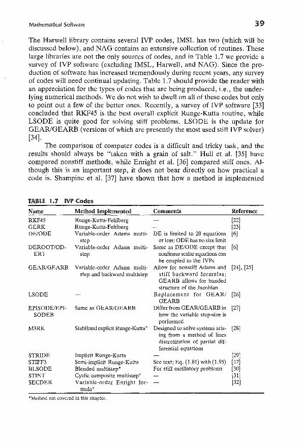
The Harwell library contains several IVP codes, IMSL has two (which will bediscussed below), and NAG contains an extensive collection of routines. Theselarge libraries are not the only sources of codes, and in Table 1.7 we provide asurvey of IVP software (excluding IMSL, Harwell, and NAG). Since the production of software has increased tremendously during recent years, any surveyof codes will need continual updating. Table 1.7 should provide the reader withan appreciation for the types of codes that are being produced, i.e., the underlying numerical methods. We do not wish to dwell on all of these codes but onlyto point out a few of the better ones. Recently, a survey of IVP software [33]concluded that RKF45 is the best overall explicit Runge-Kutta routine, whileLSODE is quite good for solving stiff problems. LSODE is the update forGEAR/GEARB (versions of which are presently the most used stiff IVP solver)[34].
The comparison of computer codes is a difficult and tricky task, and theresults should always be "taken with a grain of salt." Hull et al. [35] havecompared nonstiff methods, while Enright et al. [36] compared stiff ones. Although this is an important step, it does not bear directly on how practical acode is. Shampine et al. [37] have shown that how a method is implemented
TABLE. 1.1 (VI' Codes
[22][23]
DE is limited to 20 equations [6]or less: ODE has no size limit
Same as DE/ODE except that [6]nonlinear sclliar equations canbe coupled to the IVPs
Allow for nonstiff Adams and [24], [25]stiff backward formulas;GEARB allows for bandedstructure of the Jacobian
Replacement for GEAR/ [26]GEARB
Differ from GEARIGEARB in [27]how the variable step-size isperformed
Designed to solve systems aris- [28]ing from a method of linesdiscretization of partial differential equations
Name
RKF45GERKDE/ODE
DEROOT/ODERT
GEARIGEARB
LSODE
EPISODE/EPISODEB
M3RK
STRIDESTIFF3BLSODESTINTSECDER
Method Implemented
Runge-Kutta-FehlbergRunge-Kutta-FehlbergVariable-order Adams multi-
stepVariable-order Adams multi
step
Variable-order Adams multistep and backward multistep
Same as GEARIGEARB
Stabilized explicit Runge-Kutta*
Implicit Runge-KuttaSemi-implicit Runge-KuttaBlended multistep'Cyclic composite multistep'Variable-order Enright for-
mula'
Comments
See text; Eq. (1.81) with (1.95)For stiff oscillatory problems
Reference
[29][17][30][31][32]
*Method not covered in this chapter.
40 Initial-Value Problems for Ordinary Differential Equations
may be more important than the choice of method, even when dealing with thebest codes. There is a distinction between the best methods and the best codes.In [31] various codes for nonstiff problems are compared, and in [38] GEARand EPISODE are compared by the authors. One major aspect of code usagethat cannot be tested is the user's attitude, including such factors as user timeconstraints, accessibility of the code, familiarity with the code, etc. It is typicallythe user's attitude which dictates the code choice for a particular problem, notthe question of which is the best code. Therefore, no sophisticated code comparison will be presented. Instead, we illustrate the use of software packages bysolving two problems. These problems are chosen to demonstrate the conceptof stiffness.
The following codes were used in this study:
1. IMSL-DVERK: Runge-Kutta solver.
2. IMSL-DGEAR: This code is a modified version of GEAR. Two methodsare available in this package: a variable-order Adams multistep method anda variable-order implicit multistep method. Implicit methods require Jacobian calculations, and in this package the Jacobian can be (a) user-supplied, (b) internally calculated by finite differences, or (c) internally calculated by a diagonal approximation based on the directional derivative(for more explanation see [24]). The various methods are denoted by theparameter MF, where
MF
10212223
Method
AdamsImplicitImplicitImplicit
Jacobian
User-suppliedFinite differencesDiagonal approximation
3. STIFF3: Implements (1.81) using (1.94) and (1.95) to govern the step-sizeand error.
4. LSODE: updated version of GEAR. The parameter MF is the same as forDGEAR. MF = 23 is not an option in this package.
5. EPISODE: A true variable step-size code based on GEAR. GEAR, DGEAR,and LSODE periodically change the step-size (not on every step) in orderto decrease execution time while still maintaining accuracy. EPISODE adaptsthe step-size on every step (if necessary) and is therefore good for problemsthat involve oscillations. For decaying or linear problems, EPISODE wouldprobably require larger execution times than GEAR, DGEAR, or LSODE.
6. ODE: Variable-order Adams multistep solver.
Mathematical Software 41
(1.96)
We begin our discussions by solving the reactor problem outlined in Example 5:
dy [3.21]dx = -0.1744 exp T* Y
dT* [3.21]dx = 0.06984 exp T* Y
Y = T* = 1 at x = 0
Equations (1.96) are not stiff (see Example 1.5), and all of the codes performedthe integration with only minor differences in their solutions. Typical results areshown in Table 1.8. Notice that a decrease in TOL when using DVERK didproduce a change in the results (although the change was small). Practicallyspeaking, any of the solutions presented in Table 1.8 would be acceptable. Fromthe discussions presented in this chapter, one should realize that DVERK, ODE,DGEAR (MF = 10), LSODE (MF = 10), and EPISODE (MF = 10) usemethods that are capable of solving nonstiff problems, while STIFF3, DGEAR(MF = 21,22,23), LSODE (MF = 21,22), and EPISODE (MF = 21,22,23)implement methods for solving stiff systems. Therefore, all of the codes aresuitable for solving (1.96). One might expect the stiff problem solvers to requirelonger execution times because of the Jacobian calculations. This behavior wasobserved, but since (1.96) is a small system, i.e., two equations, the executiontimes for all of the codes were on the same order of magnitude. For a largerproblem the effect would become significant.
Next, we consider a stiff problem. Robertson [39] originallyproposed the
TABU 1.8 Typical Results from Software Packages Using Eq. (1.96)
x
0.00.10.20.30.40.50.60.70.80.91.0
DVERK,TaL = (-4)
y T*1.000000 1.000000.699795 1.120210.528839 1.188680.413483 1.234870.329730 1.268410.266347 1.293790.217094 1.313520.178118 1.329120.146869 1.341640.121569 1.351770.100931 1.36003
DVERK,TaL = (-6)
y T*1.000000 1.000000.700367 1.119990.529199 1.188530.413737 1.234770.329919 0.268330.266492 1.293730.217208 1.313470.178209 1.329090.146943 1.341610.121629 1.351750.100980 1.36002
DGEAR(MF = 21),TaL = (-4)
Y T*1.000000 1.000000.700468 1.119940.529298 1.188490.413775 1.234750.329864 1.268360.266349 1.293790.217070 1.313530.178076 1.329140.146801 1.341670.121495 1.351800.100864 1.36006
STIFF3,TaL = (-4)
Y T*1.000000 1.000000.700371 1.119980.529208 1.188530.413745 1.234770.329924 1.268330.266497 1.293730.217211 1.313470.178212 1.329090.146945 1.341610.121630 1.351750.100982 1.36001
42 Initial-Value Problems for Ordinary Differential Equations
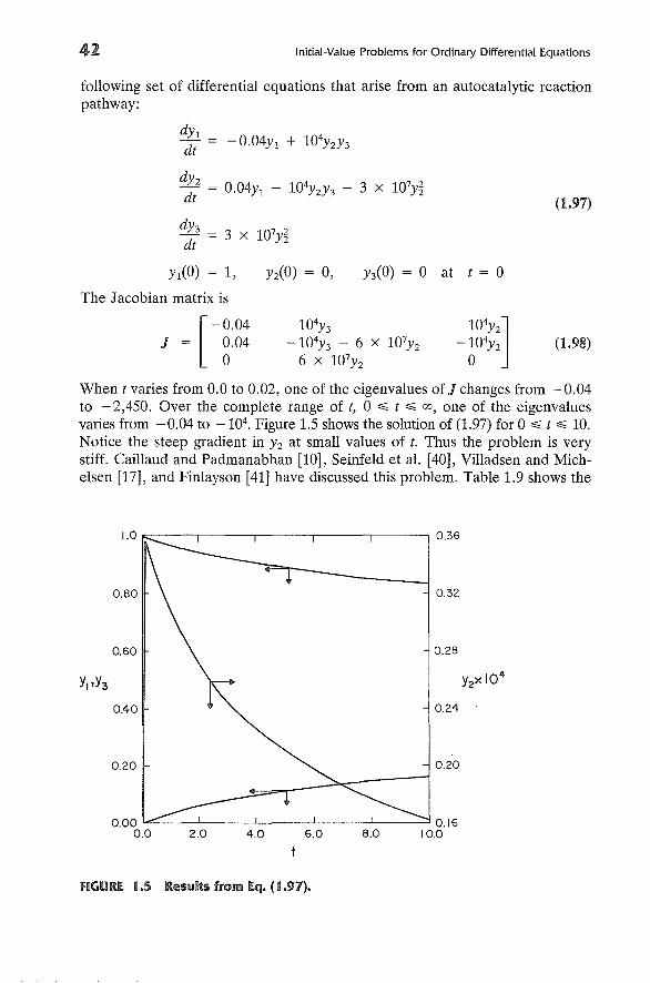
following set of differential equations that arise from an autocatalytic reactionpathway:
dYl =dt - 0.04Yl + 104YzY3
dYzdt = 0.04Yl - 104YzY3 - 3 X 10⁷y~
dY3 = 3 X 10⁷y~dt
(1.97)
The Jacobian matrix is
Yz(O) = 0, Y3(0) = 0 at t = 0
[
-0.04
J = ~.04
104Y3-104Y3 - 6 X 10⁷Yz
6 X 10⁷Yz(1.98)
When t varies from 0.0 to 0.02, one of the eigenvalues of J changes from - 0.04to -2,450. Over the complete range of t, 0 ~ t ~ 00, one of the eigenvaluesvaries from -0.04 to -104• Figure 1.5 shows the solution of (1.97) for 0 ~ t ~ 10.Notice the steep gradient in Yz at small values of t. Thus the problem is verystiff. Caillaud and Padmanabhan [10], Seinfeld et al. [40], Villadsen and Michelsen [17], and Finlayson [41] have discussed this problem. Table 1.9 shows the
i.0 ~--r------,-----,------,-------,0.36
0.80
0.60
0.40
0.20
0.32
0.28
0.24
0.20
0.00 '"""'-----'-----'-----'------''------' 0.160.0 2.0 4.0 6.0 8.0 10.0
fiGURE 1.5 Results from Eq. (1.97).
Mathematical Software 43
results at t = 10. At a TOL of 10 -4 all of the nonstiff methods failed to producea solution. At smaller tolerance values, the nonstiff methods failed to producea solution or required excessive execution times, i.e., two orders of magnitudegreater than those of the stiff methods. This behavior is due to the fact that thetolerances were too large to achieve a stable solution (recall that the step-sizeis adapted to meet the error criterion that is governed by the value of TOL) ora solution was obtained but at a high cost (large execution time) because of thevery small step-size requirements of nonstiff methods (see section on stiffness).
TABU 1.9 Comparison of Software Packages on the Robertson Problem(Results at t = 10)
ExecutionTime Ra-
Code MF TOL YI Yz X 104 Y3 tiotDVERK ( -4) No solutionDVERK (-6) No solutionDVERK ( -8) No solutionODE ( -4) No solutionODE ( -6) 0.8411 0.1586 0.1589 339.0ODE ( -9) 0.8414 0.1623 0.1586 347.0DGEAR 10 ( -4) No solutionDGEAR 21 ( -4) 0.8414 0.1624 0.1586 0.25DGEAR 22 ( -4) 0.8414 0.1624 0.1586 1.0DGEAR 23 ( -4) No solutionDGEAR 10 ( -6) 0.8414 0.1619 0.1586 261.0DGEAR 21 ( -6) 0.8414 0.1623 0.1586 1.0DGEAR 22 ( -6) 0.8414 0.1623 0.1586 1.0DGEAR 23 ( -6) 0.8414 0.1624 0.1586 2.5LSODE 10 ( -4) No solutionLSODE 21 ( -4) No solutionLSODE 22 ( -4) No solutionLSODE:j: 10 ( -4) No solutionLSODE:j: 21 ( -4) 0.8414 0.1623 0.1586 1.75LSODE:j: 22 ( -4) 0.8414 0.1623 0.1586 1.75LSODE 10 ( -6) No solutionLSODE 21 ( -6) 0.8414 0.1623 0.1586 1.75LSODE 22 ( -6) 0.8414 0.1623 0.1586 1.75EPISODE 10 ( -4) No solutionEPISODE 21 ( -4) No solutionEPISODE 22 ( -4) No solutionEPISODE 23 ( -4) No solutionEPISODE 10 ( -6) 0.8414 0.1623 0.1586 530.0EPISODE 21 ( -6) 0.8414 0.1623 0.1586 1.5EPISODE 22 ( -6) 0.8414 0.1623 0.1586 1.5EPISODE 23 ( -6) 0.8414 0.1623 0.1586 3.8STIFF3 ( -4) 0.8414 0.1623 0.1586 1.25STIFF3 ( -6) 0.8414 0.1623 0.1586 3.0"EXACT"§ 0.841 0.162 0.159
tExecution time ratio = execution time/execution time of DGEAR [MF = 21, TOL = (-6)].
+Tolerance for Y2 is (-8); for YJ and Y3, (-4).
§Caillaud and Padmanabhan [10].
44 Initial-Value Problems for Ordinary Differential Equations
TABU 1.10 Comparison of Code Results to the "Exad" Solution for Time = 1, 4,and 10
Code MF TOL t Yt Y2X 104Y3
"EXACT" 1.0 0.966 0.307 0.03354.0 0.9055 0.224 0.0944
10.0 0.841 0.162 0.159STIFF3 ( -6) 1.0 0.9665 0.3075 0.3351( -1)
4.0 0.9055 0.2240 0.9446( -1)10.0 0.8414 0.1623 0.1586
EPISODE 21 ( -6) 1.0 0.9665 0.3075 0.3351( -1)4.0 0.9055 0.2240 0.9446( -1)
10.0 0.8414 0.1623 0.1586DGEAR 10 ( -6) 1.0 0.9665 0.3087 0.3350( -1)
4.0 0.9055 0.2238 0.9445( -1)10.0 0.8414 0.1619 0.1586
DGEAR 21 ( -6) 1.0 0.9665 0.3075 0.3351( -1)4.0 0.9055 0.2240 0.9446( -1)
10.0 0.84414 0.1623 0.1586ODE ( -6) 1.0 0.9665 0.3075 0.3351( -1)
4.0 0.9055 0.2222 0.9452( -1)10.0 0.8411 0.1586 0.1589
All of the stiff algorithms were able to produce solutions with executiontimes on the same order of magnitude. Caillaud and Padmanabhan [10] havestudied (1.97) using Runge-Kutta algorithms. Their "exact" results (fourth-orderRunge-Kutta with step-size = 0.001) and the results obtained from various codesare presented in Table 1.10. Notice that when a solution was obtained fromeither a stiff or a nonstiff algorithm, the results were excellent. Therefore, thedifference between the stiff and nonstiff algorithms was their execution times.
The previous two examples have illustrated the usefulness of the commercial software packages for the solution of practical problems. It can beconcluded that generally one should use a package that incorporates an implicitmethod for stiff problems and an explicit method for nonstiff problems (this wasstated in the section on stiffness, but no examples were given).
We hope to have eliminated the "blackbox" approach to the use of initialvalue packages through the illustration of the basic methods and rationale behindthe production of these programs. No code is infallible, and when you obtainspurious results from a code, you should be able to rationalize your data withthe aid of the code's documentation and the material presented in this chapter.
PROBLEMS*
1. A tubular reactor for a homogeneous reaction has the following dimensions: L = 2 m, R = 0.1 m. The inlet reactant concentration isCo = 0.03 kmole/m3 , and the inlet temperature is To = 700 K. Other
* See the Preface regarding classes of problems.
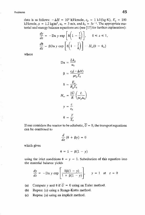
Problems 45
y = 1 at z = 0
data is as follows: - 6.H = 104 kJ/kmole, Cp = 1 kJ/(kg'K), Ea = 100kJ/kmole, P = 1.2 kglm3 , Uo = 3 mis, and ko = 5s- 1
. The appropriate material and energy balance equations are (see [17] for further explanation):
~ = - Da y exp [8(1 - ~)l 0~ z ~ 1,
~: = ~Da y exp [8(1 - ~)] - Hw (8 - 8w )
where
LkoDa=Uo
Cy=
Co
T8 =-
To
Ifone considers the reactor to be adiabatic, U = 0, the transport equationscan be combined to
d- (8 + ~y) = 0dz
which gives
8 = 1 + ~(1 - y)
using the inlet conditions 8 = Y = 1. Substitution of this equation intothe material balance yields
dy [ 8~(1 - y) ]dz = - Da y exp 1 + ~(1 _ y) ,
(a) Compute y and 8 if U = 0 using an Euler method.
(I» Repeat (a) using a Runge-Kutta method.
(c) Repeat (a) using an implicit method.
= r(x, y)
46 Initial-Value Problems for Ordinary Differential Equations
(d) Check algorithms (a) to (c) by comparing their solutions to theanalytical solution by letting 8 = O.
2. Write a subroutine called EULER such that the call is
CAll EULER (FUNC, XO, XOUT, H, TOl, N, V),where
FUNC = external subroutine to calculate the right-hand-side functions
XO = initial value of the independent variable
XOUT = final value of the independent variable
H = initial step-size
TOL = local error tolerance
N = number of equations to be integrated
Y = vector with N components for the dependent variable y. Oninput y is the vector initial values, on output it contains thecomputed values of y at XOUT.
The routine is to perform an Euler integration on
dy
dx
yeO) = Yo, XO ~ X ~ XOUT
Create this algorithm such that it contains an error-checking routine anda step-size selection routine. Test your routine by solving Example 5.Hopefully, this problem will give the reader some feel for the difficultyin creating a general-purpose routine.
3.* Repeat Problem 1, but now allow for heat transfer byletting U = 70 J/(m2 ·s·K). Locate the position of the hot spot,8max , with 8w = 1.
4.* In Example 4 we evaluated a binary batch distillation system. Now consider the same system with recycle (R = recycle ratio) and a constantcondenser hold-up M (see Figure 1.6).
Still
FIGURE 1.6 Batch still with recycle.
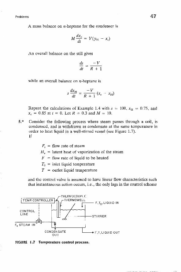
Problems
A mass balance on n-heptane for the condenser is
M dxc = V (YH - xJdt
An overall balance on the still gives
41
ds
dt
-V=---
R + 1
while an overall balance on n-heptane is
Repeat the calculations of Example 1.4 with sXc = 0.85 at t = O. Let R = 0.3 and M = 10.
0.75, and
5.* Consider the following process where steam passes through a coil, iscondensed, and is withdrawn as condensate at the same temperature inorder to heat liquid in a well-stirred vessel (see Figure 1.7).If
Fs flow rate of steam
H v latent heat of vaporization of the steam
F flow rate of liquid to be heated
To inlet liquid temperature
T outlet liquid temperature
and the control valve is assumed to have linear flow characteristics suchthat instantaneous action occurs, i.e., the only lags in the control scheme
TEMP. CONTROLLER
CONTROLLINE
THERMOCOUPLETHERMOWELLfI F,To,L1QUID IN
/-----+--STI RRER
Fs STEAM IN
CONDENSATEOUT
F,T,L1QUID OUT
FlGURf 1.1 Temperature control process.
48 Initial-Value Problems for Ordinary Differential Equations
occur in the temperature measures, then the process can be described by
dTMcp dt = FCp(To - T) + FsHv
C dTw - ( )I dt - UIAI T - Tw
C dTt - U ( )z dt - zAz Tw - Tt
Fs = Kp(Ts - Tt)
For convenience allow
(liquid energy balance)
(thermowell energy balance)
(thermocouple energy balance)
(proportional control)
F1 min- 1-
M
Hv= 1°C/kg
Mcp
To = SO°C
10 UIAI = UzAz = 1 min- l
CI Cz
The system of differential equations becomes
dTdi = Fs - T + To
dTtdt = Tw - T t
Fs = Kp(Tt - Ts)
Initially T = SO°C. Investigate the temperature response, T(t), to a lOoCstep increase in the designed liquid temperature, Ts = 60°C, for Kp = 2and Kp = 6. Recall that with proportional control there is offset in theresponse.
6.* In a closed system of three components, the following reaction path canoccur:
k3
2B~ C + B
References
with governing differential equations
49
dCA
dt
dCBdt
dCcdt
7.
Calculate the reaction pathway for k 1 = 0.08, k2
k3 = 6 X 10⁷ .
Develop a numerical procedure to solve
d2f + ~ df = <1PR(f) 0 ~ r ~ 1
dr2 r dr '
%(0) = 0, f(l) = 1
2 X 10⁴ , and
Hint: Let df/dr(l) = ex and choose ex to satisfy (df/dr) (0) = O.
(Later in this text we will discuss this method for solving boundary-valueproblems. Methods of this type are called shooting methods.)
REfERENCES
1. Conte, S. D., and C. deBoor, Elementary Numerical Analysis: An Algorithmic Approach, 3rd Ed., McGraw-Hill, New York (1980).
2. Kehoe, J. P. G., and J. B. Butt, "Interactions of Inter- and IntraphaseGradients in a Diffusion Limited Catalytic Reaction," A.I.Ch.E. J., 18,347 (1972).
3. Price, T. H., and J. B. Butt, "Catalyst Poisoning and Fixed Bed ReactorDynamics-II," Chern. Eng. Sci., 32, 393 (1977).
4. Gear, C. W., Numerical Initial-Value Problems in Ordinary DifferentialEquations, Prentice-Hall, Englewood Cliffs, N.J. (1971).
5. Johnston, R. L., Numerical Methods-A Software Approach, Wiley, NewYork (1982).
6. Shampine, L. F., and M. K. Gordon, Computer Solution of OrdinaryDifferential Equations: The Initial Value Problem, Freeman, San Francisco(1975).

50 Initial-Value Problems for Ordinary Differential Equations
7. Rosenbrock, H. H., "Some General Implicit Processes for the NumericalSolution of Differential Equations," Comput. J., 5, 329 (1963).
8. Calahan, D., "Numerical Considerations in the Transient Analysis andOptimal Design of Nonlinear Circuits," Digest Record of Joint Conferenceon Mathematical and Computer Aids to Design, ACM/SIAM/IEEE, Anaheim, Calif. 129 (1969).
9. Allen, R. H., "Numerically Stable Explicit Integration Techniques Usinga Linearized Runge-Kutta Extension," Boeing Scientific LaboratoriesDocument Dl-82-0929 (1969).
10. Caillaud, J. B., and L. Padmanabhan, "An Improved Semi-implicit RungeKutta Method for Stiff Systems," Chern. Eng. J., 2, 227 (1971).
11. Norsett, S. P., "One-Step Methods of Hermite-type for Numerical Integration of Stiff Systems," BIT, 14, 63 (1974).
12. Alexander, R., "Diagonally Implicit Runge-Kutta Methods for Stiff ODES,"SIAM J. Numer. Anal., 14, 1006 (1977).
13. Bui, T. D., and T. R. Bui, "Numerical Methods for Extremely Stiff Systems of Ordinary Differential Equations," Appl. Math. Modelling, 3, 355(1979).
14. Burka, M. K., "Solution of Stiff Ordinary Differential Equations by Decomposition and Orthogonal Collocation," A.1.Ch.E.J., 28, 11 (1982).
15. Lambert, J. D., "Stiffness," in Computational Techniques for OrdinaryDifferential Equations, 1. Gladwell, and D. K. Sayers (eds.), Academic,London (1980).
16. Michelsen, M. L., "An Efficient General Purpose Method for the Integration of Stiff Ordinary Differential Equations," A.1.Ch.E.J., 22, 594(1976).
17. Villadsen, J., and M. L. Michelsen, Solution of Differential Equation Modelsby Polynomial Approximation, Prentice-Hall, Englewood Cliffs, N.J. (1978).
18. Krogh, F. T., "Algorithms for Changing Step Size," SIAM J. Numer.Anal., 10, 949 (1973).
19. International Mathematics and Statistics Libraries Inc., Sixth Floor-NBCBuilding, 7500 Bellaire Boulevard, Houston, Tex.
20. Numerical Algorithms Group (USA) Inc., 1250 Grace Court, DownersGrove, Ill.
21. Harwell Subroutine Libraries, Computer Science and Systems Division ofthe United Kingdom Atomic Energy Authority, Harwell, England.
22. Forsythe, G. E., M. A. Malcolm, and C. B. Moler, Computer Methodsfor Mathematical Computations, Prentice-Hall, Englewood Cliffs, N.J.(1977).
23. Shampine, L. F., and H. A. Watts, "Global Error Estimation for OrdinaryDifferential Equations," ACM TOMS, 2, 172 (1976).
References 51
24. Hindmarsh, A. c., "GEAR: Ordinary Differential Equation System Solver," Lawrence Livermore Laboratory Report UCID-30001 (1974).
25. Hindmarsh, A. C., "GEARB: Solution of Ordinary Differential EquationsHaving Banded Jacobians," Lawrence Livermore Laboratory Report UCID30059 (1975).
26. Hindmarsh, A. C., "LSODE and LSODI, Two New Initial Value OrdinaryDifferential Equation Solvers," ACM SIGNUM Newsletter December(1980).
27. Byrne, G. D., and A. C. Hindmarsh, "EPISODEB: An ExperimentalPackage for the Integration of Systems of Ordinary Differential Equationswith Banded Jacobians," Lawrence Livermore Laboratory Report UCID30132 (1976).
28. Verwer, J. G., "Algorithm 553. M3RK, An Explicit Time Integrator forSemidiscrete Parabolic Equations," ACM TOMS, 6, 236 (1980).
29. Butcher, J. C., K. Burrage, and F. H. Chipman, "STRIDE Stable RungeKutta Integrator for Differential Equations," Report Series No. 150, Department of Mathematics, University of Auckland, New Zealand (1979).
30. Skeel, R., and A. Kong, "Blended Linear Multistep Methods," ACMTOMS, 3, 326 (1977).
31. Tendler, J. M., T. A. Bickart, and Z. Picel, "Algorithm 534. STINT: STiffINTegrator," ACM TOMS, 4, 399 (1978).
32. Addison, C. A., "Implementing a Stiff Method Based Upon the SecondDerivative Formulas," University of Toronto Department of ComputerScience, Technical Report No. 130/79 (1979).
33. Gladwell, 1., J. A. 1. Craigie, and C. R. Crowther, "Testing Initial-ValueProblem Subroutines as Black Boxes," Numerical Analysis Report No.34, Department of Mathematics, University of Manchester, Manchester,England.
34. Gaffney, P. W., "Information and Advice on Numerical Software," OakRidge National Laboratory Report No. ORNL/CSD/TM-147, May (1981).
35. Hull, T. E., W. H. Enright, B. M. Fellen, and A. E. Sedgwick, "Comparing Numerical Methods for Ordinary Differential Equations," SIAMJ. Numer. Anal., 9, 603 (1972).
36. Enright, W. H., T. E. Hull, and B. Lindberg, "Comparing NumericalMethods for Stiff Systems of ODEs," BIT, 15, 10 (1975).
37. Shampine, L. F., H. A. Watts, and S. M. Davenport, "Solving NonstiffOrdinary Differential Equations-The State of the Art," SIAM Rev., 18,376 (1976).
38. Byrne, G. D., A. C. Hindmarsh, K. R. Jackson, and H. G. Brown, "AComparison of Two ODE CODES: GEAR and ERISODE," Comput.Chern. Eng., 1, 133 (1977).
52 Initial-Value Problems for Ordinary Differential Equations
39. Robertson, A. H., "Solution of a Set of Reaction Rate Equations," inNumerical Analysis, J. Walsh (ed.), Thomson Brook Co., Washington(1967).
40. Seinfeld, J. H., L. Lapidus, and M. Hwang, "Review of Numerical Integration Techniques for Stiff Ordinary Differential Equations," Ind. Eng.Chern. Fund., 9, 266 (1970).
41. Finlayson, B. A., Nonlinear Analysis in Chemical Engineering, McGrawHill, New York (1980).
BIBLIOGRAPHY
Only a brief overview of IVPs has been given in this chapter. For additional or moredetailed information, see the following:
Finlayson, B. A., Nonlinear Analysis in Chemical Engineering, McGraw-Hill, New York(1980).
Forsythe, G. E., M. A. Malcolm, and C. B. Moler, Computer Methods for MathematicalComputations, Prentice-Hall, Englewood Cliffs, N.J. (1977).
Gear, C. W., Numerical Initial-Value Problems in Ordinary Differential Equations, Prentice-Hall, Englewood Cliffs, N.J. (1971).
Hall, G., and J. M. Watt (eds.), Modern Numerical Methods for Ordinary DifferentialEquations, Clarendon Press, Oxford (1976).
Johnston, R. L., Numerical Methods-A Software Approach, Wiley, New York (1982).
Lambert, J. D., Computational Methods in Ordinary Differential Equations, Wiley, NewYork (1973).
Shampine, L. F., and M. K. Gordon, Computer Solution of Ordinary Differential Equations: The Initial Value Problem, Freeman, San Francisco (1975).
Villadsen, J., and M. L. Michelsen, Solution of Differential Equation Models by Polynomial Approximation, Prentice-Hall, Englewood Cliffs, N.J. (1978).
Boundary-Value ProblemsOrdinary Differential Equations:Discrete Variable Methods
INTRODUCTION
In this chapter we discuss discrete variable methods for solving BVPs for ordinarydifferential equations. These methods produce solutions that are defined on aset of discrete points. Methods of this type are initial-value techniques, i.e.,shooting and superposition, and finite difference schemes. We will discuss initialvalue and finite difference methods for linear and nonlinear BVPs, and thenconclude with a review of the available mathematical software (based upon themethods of this chapter).
BACKGROUND
One of the most important subdivisions of BVPs is between linear and nonlinearproblems. In this chapter linear problems are assumed to have the form
y' = F(x)y + z(x), a < x < b (2.1a)
with
A yea) + B y(b) = 'Y (2.1b)
where 'Y is a constant vector, and nonlinear problems to have the form
y' = f(x,y), a < x < b (2.2a)
53
54 Boundary-Value Problems for Ordinary Differential Equations: Discrete Variable Methods
with
g(y(a), y(b» = 0 (2.2b)
If the number of differential equations in systems (2.1a) or (2.2a) is n, then thenumber of independent conditions in (2.1b) and (2.2b) is n.
In practice, few problems occur naturally as first-order systems. Most areposed as higher-order equations that can be converted to a first-order system.All of the software discussed in this chapter require the problem to be posed inthis form.
Equations (2.1b) and (2.2b) are called boundary conditions (BCs) sinceinformation is provided at the ends of the interval, i.e., at x = a and x = b.The conditions (2.1b) and (2.2b) are called nonseparated BCs since they caninvolve a combination of information at x = a and x = b. A simpler situationthat frequently occurs in practice is that the BCs are separated; that is, (2.1b)and (2.2b) can be replaced by
A y(a) = "h, B y(b) = "/2 (2.3)
where "h and "12 are constant vectors, and
giy (b» = 0 (2.4)
respectively, where the total number of independent conditions remains equalto n.
INITIAL-VALLIE METHODS
Shooting Methods
We first consider the single linear second-order equation
Ly == - y" + p(x)y' + q(x)y = r(x),
with the general linear two-point boundary conditions
aoy(a) - aly'(a) = Ct
boy(b) + bly'(b) = [3
a<x<b (2.5a)
(2.5b)
(2.5c)
where ao, alJ Ct, bo, blJ and [3 are constants, such that
aOal ;;;: 0, laol + lall =1= °bobl ;;;: 0, Ibol + Ibll =1= °
laol + Ibol =1= °We assume that the functions p(x), q(x), and r(x) are continuous on [a, b] andthat q(x) > 0. With this assumption [and (2.Sc)] the solution of (2.5) is unique
Initial-Value Methods 55
[1]. To solve (2.5) we first define two functions, y(l) (x) and y(Z) (x), on [a, b]as solutions of the respective initial-value problems
Ly<l) = rex),
Ly<Z) = 0,
y(l)(a) = - aClJ
y(Z)(a) = alJ
y(1)' (a) = - aCo
y(Z)' (a) = ao
(2.6a)
(2.6b)
where Co and Cl are any constants such that
alCO - aOCl = 1
The function y(x) defined by
y(x) == y(x; s) = y(l)(X) + sy(Z) (x), a~x~b
(2.7)
(2.8)
satisfies aoy(a) - aly'(a) = a(alCO- aOCl ) = a, and will be a solution of (2.5)if s is chosen such that
<p(s) = boy(b; s) + bly'(b; s) - 13 = 0
This equation is linear in s and has the single root
13 - [bOy<l)(b) + bl y(1)'(b)]s =
[boy(Z)(b) + bly(Z)'(b)]
Therefore, the method involves:
(2.9)
(2.10)
1. Converting the BVP into an IVPby specifying extra initial conditions
2. Guessing the initial conditions andsolving the IVP over the entire interval
3. Solving for s and constructing y.
1. (2.5) to (2.6)
2. Guess Co, evaluate Cl from (2.7),and solve (2.6)
3. Evaluate (2.10) for s; use sin (2.8)
(2.11)
The shooting method consists iIi simply carrying out the above procedurenumerically; that is, compute approximations to y<1) (x) , y(1)'(x), y(Z) (x) , y(Z)'(x)and use them in (2.8) and (2.10). To solve the initial-value problems (2.6), firstwrite them as equivalent first-order systems:
[ :(~:], = [;~~l) + qW(l) - r]
w(1)(a) = -aClJ v(l)(a) = -aCo
and
[w(Z)]' [v(Z) ]v(Z) = pv(Z) + qw(Z)
w(Z)(a) = alJ v(Z)(a) = ao
(2.12)
56 Boundary-Value Problems for Ordinary Differential Equations: Discrete Variable Methods
respectively. Now any of the methods discussed in Chapter 1 can be employedto solve (2.11) and (2.12).
Let the numerical solutions of (2.11) and (2.12) be
At the point Xo = a, the exact data can be used so that
W (l) - -"'C W(2) - -"'Co- ..... v 0- ..... 0
respectively, for
W(I) V(l) W(2) V(2)l' l' l' l'
Xi = a + ih,
b - ah=-
N
V(l) = ao 1,
i = 0,1, ... ,N
i = 0,1, ... ,N
V (2) - ao - 0
(2.13)
(2.14)
To approximate the solution y(x), set
y. = W(I) + SW(2)l l l
where
Yi = y(x;)
S = 13 - [boWjJ) + b1VjJ)]
[boWZ) + b1VZ)]
(2.15)
(2.16)
This procedure can work well but is susceptible to round-off errors. If W~l) andW~2) in (2.15) are nearly equal and of opposite sign for some range of i values,cancellation of the leading digits in Yi can occur.
Keller [1] posed the following example to show how cancellation of digitscan occur. Suppose that the solution of the IVP (2.6) grows in magnitude asX ~ b and that the boundary condition at x = b has b1 = °[y(b) = 13 isspecified]. Then if 1131«lboWjJ)1
and
S=W(l)
N---W(2)
N
(2.17)
[W(1)]Y. = W(1) - ~ W(2)
l l W(2) l
N
(2.18)
Clearly the cancellation problem occurs here for Xi near b. Note that the solutionW~l) need not grow very fast, and in fact for 13 = °the difficulty is alwayspotentially present. If the loss of significant digits cannot be overcome by theuse of double precision arithmetic, then multiple-shooting techniques (discussedlater) can be employed.
Initial-Value Methods
We now consider a second-order nonlinear equation of the form
y" = f(x, y, y'), a < x < b
subject to the general two-point boundary conditions
aoy(a) - aly' (a) = a,
boy(b) + bly'(b) = (3,
ao + bo > 0
The related IVP is
57
(2.19a)
(2.19b)
where
u" = f(x, u, u'),
u(a) = als - cla
u'(a) = aos - coa
a<x<b (2.20a)
(2.20b)
The solution of (2.20), u = u(x; s), will be a solution of (2.19) if s is a root of
<!>(s) = bou(b; s) + blu'(b; s) - (3 = 0 (2.21)
To carry out this procedure numerically, convert (2.20) into a first-order system:
with
w(a) = als - cla
v(a) = aos - coa
In order to find s, one can apply Newton's method to (2.21), giving
s[k+ll = s[kl _ <!>(s[kl)<!>'(s[kl)' k = 0, 1, ...
s[OI = arbitrary
To find <!>'(s), first define
t() aw(x; s) d () av(x; s)."x= an T)X=as as
Differentiation of (2.22) with respect to s gives
(2.22a)
(2.22b)
(2.23)
(2.24)
f = T),
T) , = af T) + af £,av aw
T)(a) = ao
(2.25)
58 Boundary-Value Problems for Ordinary Differential Equations: Discrete Variable Methods
Solution of (2.25) allows for calculation of <\>' as
<\>' = bo i;(b; s) + bi T)(b; s) (2.26)
Therefore, the numerical solution of (2.25) would be computed along with thenumerical solution of (2.22). Thus, one iteration in Newton's method (2.23)requires the solution of two initial-value problems.
EXAMPLE 1
An important problem in chemical engineering is to predict the diffusion andreaction in a porous catalyst pellet. The goal is to predict the overall reactionrate of the catalyst pellet. The conservation of mass in a spherical domain gives
D[~ :r (r2 ~~)] = k9l(e), 0 < r < rp
where
r = radial coordinate (rp = pellet radius)
D = diffusivity
e = concentration of a given chemical
k = rate constant
9l(e) = reaction rate function
with
de
dro at r = 0 (symmetry about the origin)
e = Co at r = rp (concentration fixed at surface)
If the pellet is isothermal, an energy balance is not necessary. We define theeffectiveness factor E as the average reaction rate in the pellet divided by theaverage reaction rate if the rate of reaction is evaluated at the surface. Thus
f:P
9l(e(r))r2 drE=-..,.-----f:P
9l(eo)r2 dr
We can integrate the mass conservation equation to obtain
frp [1 d ( de) ] frp
de ID - - r2 - r2 dr = k 9l(e)r2 dr = Dr2 -o r2 dr dr 0 p dr
rp
Hence the effectiveness factor can be rewritten as
3r; D ~~IE = __-,--_rp
k 9l(eo)
Initial-Value Methods 59
If E = 1, then the overall reaction rate in the pellet is equal to the surface valueand mass transfer has no limiting effects on the reaction rate. When E < 1, thenmass transfer effects have limited the overall rate in the pellet; i.e., the averagereaction rate in the pellet is lower than the surface value of the reaction ratebecause of the effects of diffusion.
Now consider a sphere (5 mm in diameter) of "{-alumina upon which Pt isdispersed in order to catalyze the dehydrogenation of cyclohexane. At 700 K,the rate constant k is 4 s-1, and the diffusivity D is 5 X 10⁻² cm2/s. Set up theequations necessary to calculate the concentration profile of cyclohexane withinthe pellet and also the effectiveness factor for a general 9r'(c). Next, solve theseequations for 9r'(c) = c, and compare the results with the analytical solution.
SOLUTION
Define
C = concentration of cyclohexaneconcentration of cyclohexane at the surface of the sphere
R = dimensionless radial coordinate based on the radius of the
sphere (rp = 2.5 mm)
Assume that the spherical pellet is isothermal. The conservation of mass equationfor cydohexane is
0< R < 1,
with
dC = 0 at R = 0 (due to symmetry)dR
C = 1 at R = 1 (by definition)
where
<1>= ,,J~ (Thiele modulus)
Since 9r' (c) is a general function of c, it may be nonlinear in c. Therefore,assume that 9r' (c) is nonlinear and rewrite the conservation equation in theform of (2.19):
d2C = <1>2 9r'(c) _ ~ dC = feR C C)
dR2 Co R dR "
60 Boundary-Value Problems for Ordinary Differential Equations: Discrete Variable Methods
The related IVP systems become
with
and
[WvJ '= v
cI>2 9l(c) _ ~ vCo R
W(O) = s,
v(O) = 0,
~(O) = 1
11(0) = °
2- -11
R
k = 0,1, ...
<p(s) w(l; s) - 1
<p'(s) ~(1; s)
Choose s[O], and solve the above system of equations to obtain a solution. Compute a new s by
S[k+l] = srk] _ w(l; s[k1) - 1
~(1; S[k]) ,
and repeat until convergence is achieved.Usingthedataprovided,wegetcI> = 2.236. If 9l(c) = c,thentheproblem
is linear and no Newton iteration is required. The IMSL routine DVERK (seeChapter 1) was used to integrate the first-order system of equations. The results,along with the analytical solution calculated from [2],
C = sinh (cI>R)R sinh (cI»
are shown in Table 2.1. Notice that the computed results are the same as theanalytical solution (to four significant figures). In Table 2.1 we also compare
TABU 2.1 Results from Example 1TOl = 10- 6 for DVERK
R
0.00.20.40.60.81.0E
C,AnalyticalSolution
0.48350.49980.55060.64220.78591.00000.7726
C,ComputedSolution(s = 0.4835)
0.48350.49980.55060.64220.78591.00000.7727
Initial-Value Methods
the computed value of E, which is defined as
dCI3 dR 1
E=-<I>2
61
with the analytical value from [2],
E - l [ 1 _ 1:-]- <I> tanh (<I» <I>
Again, the results are quite good.Physically, one would expect the concentration of cyclohexane to decrease
as R decreases since it is being consumed by reaction. Also, notice that theconcentration remains finite at R = O. Therefore, the reaction has not gone tocompletion in the center of the catalytic pellet. Since E < 1, the average reactionrate in the pellet is less than the surface value, thus showing the effects of masstransfer.
EXAMPLE 2
If the system described in Example 1 remains the same except for the fact thatthe reaction rate function now is second-order, i.e., 9P (c) = c2 , compute theconcentration profile of cyclohexane and calculate the value of the effectivenessfactor. Let Co = 1.
SOLUTION
The material balance equation is now
d2C ~ dC _ <I>2C2 0 < R < 1
dR2 + R dR - ,
dC = 0 at R = 0dR
C = 1 at R = 1
<I> = 2.236
The related IVP systems are
withw(O) = s,
v(O) = 0,
~(O) = 1
'r](0) = 0
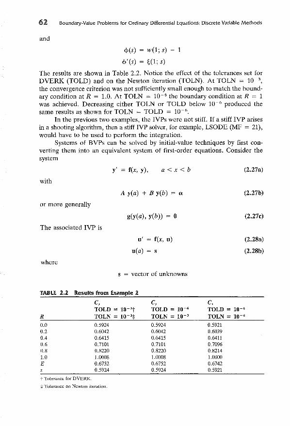
62 Boundary-Value Problems for Ordinary Differential Equations: Discrete Variable Methods
and
<I>(s) w(l; s) - 1
<1>' (s) HI; s)
The results are shown in Table 2.2. Notice the effect of the tolerances set forDVERK (TOLD) and on the Newton iteration (TOLN). At TOLN = 10- 3
,
the convergence criterion was not sufficiently small enough to match the boundary condition at R = 1.0. At TOLN = 10- 6 the boundary condition at R = 1was achieved. Decreasing either TOLN or TOLD below 10-6 produced thesame results as shown for TOLN = TOLD = 10- 6
•
In the previous two examples, the IVPs were not stiff. If a stiff IVP arisesin a shooting algorithm, then a stiff IVP solver, for example, LSODE (MF = 21),would have to be used to perform the integration.
Systems of BVPs can be solved by initial-value techniques by first converting them into an equivalent system of first-order equations. Consider thesystem
with
y' = f(x, y), a<x<b (2.27a)
or more generally
The associated IVP is
where
A yea) + B y(b) = a
g(y(a), y(b)) = 0
u' = f(x, u)
u(a) = s
s = vector of unknowns
(2.27b)
(2.27c)
(2.28a)
(2.28b)
TABLE 1.1 Results from Example 1
R
0.00.20.40.60.81.0Es
C,TOLD = 1O-3tTOLN = 10-3 :1=
0.59240.60420.64150.71010.82201.00080.67520.5924
C,TOLD = 10-6
TOLN = 10-3
0.59240.60420.64150.71010.82201.00080.67520.5924
C,TOLD = 10-6
TOLN = 10-6
0.59210.60390.64110.70960.82141.00000.67420.5921
t Tolerance for DVERK.
*Tolerance on Newton iteration.
Initial-Value Methods 63
We now seek s such that u(x; s) is a solution of (2.27). This occurs if s is a rootof the system
or more generally
<I>(s) = A s + B u(b; s) - a = 0
<I>(s) = g(s, u(b; s)) = 0
(2.29)
(2.30)
Thus far we have only discussed shooting methods that "shoot" from x = a.Shooting can be applied in either direction. If the solutions of the IVP growfrom x = a to x = b, then it is likely that the shooting method will be mosteffective in reverse, that is, using x = b as the initial point. This procedure iscalled reverse shooting.
Multiple Shooting
Previously we have discussed some difficulties that can arise when using a shooting method. Perhaps the best known difficulty is the loss in accuracy caused bythe growth of solutions of the initial-value problem. Multiple shooting attemptsto prevent this problem. Here, we outline multiple-shooting methods that areused in software libraries.
Multiple shooting is designed to reduce the growth of the solutions of theIVPs that must be solved. This is done by partitioning the interval into a numberof subintervals, and then simultaneously adjusting the "initial" data in order tosatisfy the boundary conditions and appropriate continuity conditions. Considera system of n first-order equations of the form (2.27), and partition the intervalas
O<t<l
a = Xo < Xl < ... < XN-l < XN = b
Define
for
1= 1,2, ... , N
With this change of variables, (2.27) becomes
d,,·dt' = r;(t, r;),
for
i = 1,2, ... ,N
(2.31)
(2.32)
(2.33)
64 Boundary-Value Problems for Ordinary Differential Equations: Discrete Variable Methods
The boundary conditions are now
A '1'1(0) + B'I'N(l) = a
or
[for (2.27b)]
[for (2.27c)]
(2.34a)
(2.34b)
In order to have a continuous solution to (2.27), we require
i = 1, 2, ... , N - 1 (2.35)
The N systems of n first-order equations can thus be written as
ddt lfI = aCt, lfI)
with
P lfI(O) + Q lfI(l) = 'Y
or
G = 0
wherelfI = ['I'I(t), 'I'z(t), ... , 'I'N(t)f
aCt, lfI) = [r1(t, '1'1), rzCt, 'I'z), ... , rN(t, 'I'N)f
'Y = [a, 0, , Of
o = [0, 0, , ofA
1
(2.36)
P=
Q=
. 0o
1
o B-1 0
Initial-Value Methods
The related IVP problem is
ddt V = aCt, V),
with
V(O) = 8
where
0< t < 1
65
(2.37)
The solution of (2.37) is a solution to (2.36) if 8 is a root of
«1>(8) = P 8 + Q V(l; 8) - 'Y = 0
or
«1>(8) = G = 0
(2.38)
depending on whether the BCs are of form (2.27b) or (2.27c). The solutionprocedure consists of first guessing the "initial" data 8, then applying ordinaryshooting on (2.37) while also performing a Newton iteration on (2.38). Obviously, two major considerations are the mesh selection, i.e., choosing Xi'
i = 1, ... , N - 1, and the starting guess for 8. These difficulties will be discussed in the section on software.
An alternative shooting procedure would be to integrate in both directionsup to certain matching points. Formally speaking, this method includes theprevious method as a special case. It is not clear a priori which method ispreferable [3].
Superposition
Another initial-value method is called superposition and is discussed in detailby Scott and Watts [4]. We will outline the method for the following linearequation
with
y'(x) = F(x)y(x) + g(x) ,
A yea) = Ol
B y(b) = ~
a<x<b (2.39a)
(2.39b)
The technique consists of finding a solution y(x) such that
y(x) = vex) + U(x)c (2.40)
66 Boundary-Value Problems for Ordinary Differential Equations: Discrete Variable Methods
where the matrix U satisfies
U'(x) = F(x)U(x)
A U(a) = 0
the vector vex) satisfies
v'(x) = F(x) vex) + g(x)
v(a) = a
(2.41a)
(2.41b)
(2.42a)
(2.42b)
and the vector of constants c is chosen to satisfy the boundary conditions atx = b:
B U(b)c = -B v(b) + 13 (2.43)
The matrix U(x) is often referred to as the fundamental solution, and the vectorvex) the particular solution.
In order for the method to yield accurate results, vex) and the columns ofU(x) must be linearly independent [5]. The initial conditions (2.41b) and (2.42b)theoretically ensure independence; however, due to the finite world length usedby computers, the solutions may lose their numerical independence (see [5] forfull explanation). When this happens, the resulting matrix problem (2.43) maygive inaccurate answers for c. Frequently, it is impossible to extend the precisionof the computations in order to overcome this difficulty. Therefore, the basicsuperposition method must be modified.
Analogous to using multiple shooting to overcome the difficulties withshooting methods, one can modify the superposition method by subdividing theinterval as in (2.31), and then defining a superposition solution on each subinterval by
where
yJx) = vJx) + UJx)Ci(x) ,
i = 1,2, ... ,N,
Xi-I";;; X ,,;;; Xi (2.44)
U;(x) = F(x) UJx)
Ui(Xi- l ) = Ui-l(Xi- l ), A Ul(a) = 0
v; (x) = F(x)vi(x) + g(x)
(2.45)
(2.46)
and
yJxi) = Yi+ 1(x;)
B UN(b)CN = -B vN(b) + 13
(2.47)
(2.48)
The principle of the method is then to piece together the solutions defined onthe various subintervals to obtain the desired solution. At each of the mesh
Initial-Value Methods 61
points Xi the linear independence of the solutions must be checked. One way toguarantee independence of solutions over the entire interval is to keep themnearly orthogonal. Therefore, the superposition algorithm must be coupled witha routine that checks for orthogonality of the solutions, and each time the vectorsstart to lose their linear independence, they must be orthonormalized [4,5] toregain linear independence. Obviously, one of the major problems in implementing this method is the location of the orthonormalization points Xi.
Nonlinear problems can also be solved using superposition, but they firstmust be "linearized." Consider the following nonlinear BVP:
y' (x) = f(x, y),
A y(a) = Ol
B y(b) = ~
a<x<b
(2.49)
If Newton's method is applied directly to the nonlinear function f(x, y), thenthe method is called quasilinearization. Quasilinearization of (2.49) gives
where
Y(k+l)(X) = f(x, Y(k)(X» + J(x, Y(k)(X»(Y(k+l)(X) - Y(k)(X»,
k = 0,1, ...
J(X, Y(k)(X» = Jacobian of f(x, Y(k/X»
k = iteration number
(2.50)
One iteration of (2.50) can be solved by the superposition methods outlinedabove since it is a linear system.
FINITE DIFFERENCE METHODS
Up to this point, we have discussed initial-value methods for solving boundaryvalue problems. In this section we cover finite difference methods. These methods are said to be global methods since they simultaneously produce a solutionover the entire interval.
The basic steps for a finite difference method are as follows: first, choosea mesh on the interval of interest, that is, for [a,b]
a = Xo < Xl < ... < XN < XN+l = b (2.51)
such that the approximate solution will be sought at these mesh points; second,form the algebraic equations required to satisfy the differential equation andthe BCs by replacing derivatives with difference quotients involving only themesh points; and last, solve the algebraic system of equations.
68 Boundary-Value Problems for Ordinary Differential Equations: Discrete Variable Methods
Linear Second-Order Equations
We first consider the single linear second-order equation
Ly == -y" + p(x)y' + q(x)y = rex),
subject to the Dirichlet boundary conditions
yea) = a
y(b) = f3
On the interval [a, b] impose a uniform mesh,
a<x<b (2.52a)
(2.52b)
Xi = a + ih,
b - ah=-
N + 1
i = 0, 1, ... , N + 1,
The parameter h is called the mesh-size, and the points Xi are the mesh points.If y(x) has continuous derivatives of order four, then, by Taylor's theorem,
h2 h3 h4
y(x + h) = y(x) + hy'(x) + -y"(x) + -y"'(x) + -y""(£)2! 3! 4! '
h2 h3 h4 _y(x - h) = y(x) - hy'(x) + -y"(x) - -y"'(x) + -y""(£)
2! 3! 4! '
Xi - h~~~Xi (2.54)
From (2.53) and (2.54) we obtain
y'(x) = [y(X + h) - y(X)] _ ~ y"(x) _ h2
y"'(x) _ h3
y""(£) (2.55)h 2! 3! 4!
y'(x) = [y(X) - ~(x - h)] + ;! y"(x) _ ~: y"'(x) + ~: y""(~) (2.56)
respectively. The forward and backward difference equations (2.55) and (2.56)can be written as
respectively, where
y'(x;) = Yi+\- Yi + O(h)
y'(xi) = Yi -/i-1 + O(h)
(2.57)
(2.58)
Yi = y(Xi)
Thus, Eqs. (2.57) and (2.58) are first-order accurate difference approximationsto the first derivative. A difference approximation for the second derivative is
Finite Difference Methods
obtained by adding (2.54) and (2.53) to give
h4 _
y(x + h) + y(x - h) = 2y(x) + h2y"(x) + 4! [y""(£) + y'11I(£)]
from which we obtain
"( .) = (Yi+l - 2Yi + Yi-l) + 0(h2)Y X, h2
69
(2.59)
(2.60)
(2.62)
If the BVP under consideration contains both first and second derivatives, thenone would like to have an approximation to the first derivative compatible withthe accuracy of (2.60). If (2.54) is subtracted from (2.53), then
h3 h4 _
2hy'(x) = y(x + h) - y(x - h) - 3! ylll(X) + 4! [y'lll(£) - y""(£)] (2.61)
and hence
y'(Xi) = [Yi+l ; Yi-l] + 0(h2)
which is the central difference approximation for the first derivative and is clearlysecond-order accurate.
To solve the given BVP, at each interior mesh point Xi we replace thederivatives in (2.52a) by the corresponding second-order accurate differenceapproximations to obtain
L - [Ui+ 1 - 2ui + Ui- 1 ] () [Ui+ 1 - Ui- 1 ] (hUi= - h2 + P Xi 2h + q Xi)Ui = r(xi)
i = 1, ... ,N
and
(2.63)
Uo = a,
where
The result of multiplying (2.63) by h2/2 is
h2 h2
2' Lhui = aiui- 1 + biui + CiUi+ 1 = 2'r(x;), i = 1,2, ... ,N
Uo = a, (2.64)where
ai = - ~ [1 + ~ P(Xi)]
bi = [1 + ~ q(X;)]
Ci = - ~ [1 - ~ P(Xi) ]
70 Boundal)'-Value Problems for Ordinal)' Differential Equations: Discrete Variable Methods
The system (2.64) in vector notation is
Au=r (2.65)
where
u = [u I , U2' ••. , UN]T
h2 [2al (Y 2CN I3] Tr = 2 r(x l ) - Ji2' r(X2)' ... , r(xN - I ) - h2
bl CI
a2 b2 C2 °A=
°aN - I bN - I CN - I
aN bN
A matrix of the form A is called a tridiagonal. This special form permits a veryefficient application of the Gaussian elimination procedure (described in Appendix C).
To estimate the error in the numerical solution of BVPs by finite differencemethods, first define the local truncation errors 'Ti[0] in L h as an approximationof L, for any smooth function 0(x) by
'Ti[0] = L h0(Xi) - L0(xi), i = 1, 2, ... , N (2.66)
(2.68)
(2.67)
i = 1, ... ,N
If 0(x) has continuous fourth derivatives in [a, b], then for L defined in (2.52)and L h defined in (2.63),
'Ti[0] = _ [0(Xi + h) - 20~:i) + 0(xi - h)] + 0"(xi)
( .) [0(Xi + h) - 0(xi - h) _ W( .)]+ P X, 2h )U X,
or by using (2.59) and (2.61),
'Ti[0] = - ~~ [0""(1';) - 2p(xi)0"'(;Yi)],
From (2.67) we find that L h is consistent with L, that is, 'Ti[0] -7 °as h -7 0,for all functions 0(x) having continuous second derivatives on [a, b]. Further,from (2.68), it is apparent that L h has second-order accuracy (in approximatingL) for functions 0(x) with continuous fourth derivatives on [a, b]. For sufficientlysmall h, L h is stable, i.e., for all functions Vi' i = 0, 1, ... , N + 1 defined onXi' i = 0, 1, ... , N + 1, there is a positive constant M such that
Ivil ~ M {max (Ivai, IVN+II) + max ILhvil}l~i~N
Finite Difference Methods 71
for i = 0, 1, ... , N + 1. If L h is stable and consistent, it can be shown thatthe error is given by
lUi - y(xi)1 .;;; M max ITj[y]l,1 ~ j ~ i
(for proof see Chapter 3 of [1]).
i = 1, ... , N (2.69)
Flux Boundary Conditions
Consider a one-dimensional heat conduction problem that can be described byFourier's law and is written as
where
1 d [ dT]- - zSk - = g(z),ZS dz dz
O<z<l (2.70)
k = thermal conductivity
g(z) = heat generation or removal function
s = geometric factor: 0, rectangular; 1, cylindrical; 2, spherical
In practical problems, boundary conditions involving the flux of a given component occur quite frequently. To illustrate the finite difference method withflux boundary conditions, consider (2.70) with s = 0, g(z) = z, k = constant,and
T = To at z = ° (2.71)
(2.72)
where Al and A2 are given constants. Since the governing differential equationis (2.70), the difference formula is
with
i = 1,2, ... ,N (2.73a)
(2.73b)
(2.73c)
Since UN + I is now an unknown, a difference equation for (2.73c) must be determined in order to solve for U N + I •
To determine UN+l> first introduce a "fictitious" point X N + 2 and a corresponding value U N + 2 . A second-order correct approximation for the first deriv-
72 Boundary-Value Problems for Ordinary Differential Equations: Discrete Variable Methods
ative at z = 1 is
dT TN+ 2 - TN-=dz 2h
Therefore, approximate (2.73c) by
and solve for U N + 2
(2.74)
(2.75)
(2.76)
(2.77)
UN+2 = 2h(A2 - A1UN + 1) + UN
The substitution of (2.76) into (2.73a) with i = N + 1 gives
h2
(11.2 - A1UN+1)h - UN+l + UN = 2k
Notice that (2.77) contains two unknowns, UN and UN+l' and together with theother i = 1, 2, ... , N equations of type (2.73a), maintains the tridiagonalstructure of the matrix A. This method of dealing with the flux condition is calledthe method of fictitious boundaries for obvious reasons.
EXAMPLE 3
A simple but practical application of heat conduction is the calculation of theefficiency of a cooling fin. Such fins are used to increase the area available forheat transfer between metal walls and poorly conducting fluids such as gases.A rectangular fin is shown in Figure 2.1. To calculate the fin efficiency one mustfirst calculate the temperature profile in the fin. If L > > B, no heat is lost fromthe end or from the edges, and the heat flux at the surface is given by
MetalWallTw
L
~~2B
Cooling Fin
FIGURE 2.1 Cooling fin.
Finite Difference Methods 73
q = "f)(T - Ta) in which the convective heat transfer coefficient "f) is constantas is the surrounding fluid temperature Ta, then the governing differential equation is
d 2 T "f)- = - (T - Ta)dz2 kB
where
k = thermal conductivity of the fin
and
T(O) = Tw
dT (L) = 0dz
Calculate the temperature profile in the fin, and demonstrate the order of accuracy of the finite difference method.
SOLUTION
Define
e T - Ta
Tw - Ta
e(o) = 1,
zx=-
L
H ~ j~~'The problem can be reformulated as
d 2edx2 = H
2e,de- (1) = 0dx
The analytical solution to the governing differential equation is
e = _co_s_h_H_(",-1_-_x-,-)cosh H
For this problem the finite difference method (2.63) becomes
i = 1,2, ... ,N
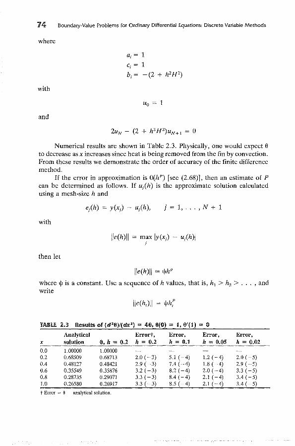
14 Boundary-Value Problems for Ordinary Differential Equations: Discrete Variable Methods
where
ai = 1Ci = 1
hi = -(2 + hZHZ)
with
Uo = 1
and
Numerical results are shown in Table 2.3. Physically, one would expect eto decrease as x increases since heat is being removed from the fin by convection.From these results we demonstrate the order of accuracy of the finite differencemethod.
If the error in approximation is O(hP ) [see (2.68)], then an estimate of Pcan be determined as follows. If uj(h) is the approximate solution calculatedusing a mesh-size hand
j = 1, ... ,N + 1
with
IIe(h)11 = max Iy(x) - uih)1j
then let
IIe(h)11 = ljJhP
where ljJ is a constant. Use a sequence of h values, that is, hI > hz > ... , andwrite
TABU 1.3 Results of(d2 0)/(dx2 ) = 46,0(0) = t, 0'(1) = 0
Analytical Errort, Error, Error, Error,x solution 0, h = 0.2 h = 0.2 h = 0.1 h = 0.05 h = 0.02
0.0 1.00000 1.000000.2 0.68509 0.68713 2.0 (-3) 5.1 (-4) 1.2 (-4) 2.0 (-5)0.4 0.48127 0.48421 2.9 (-3) 7.4(-4) 1.8 (-4) 2.9 (-5)0.6 0.35549 0.35876 3.2 (-3) 8.2 (-4) 2.0 (-4) 3.3(-5)0.8 0.28735 0.29071 3.3 (-3) 8.4(-4) 2.1 (-4) 3.4(-5)LV 0.26580 0.26917 3.3 (-3) 8.5 (-4) 2.1 (-4) 3.4 (-5)
tError = e - analytical solution.
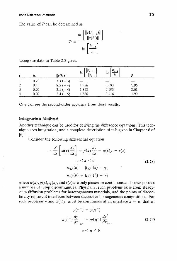
Finite Difference Methods
The value of P can be determined as
In [lle(ht - 1)11]Ile(ht)11
P=-----
In [\~1]
Using the data in Table 2.3 gives:
In[~] In [\~1]h, Ile(h,)11 Ile,ll p
1 0.20 3.3 (-3)2 0.10 8.5(-4) 1.356 0.693 1.963 0.05 2.1 (-4) 1.398 0.693 2.014 0.02 3.4(-5) 1.820 0.916 1.99
One can see the second-order accuracy from these results.
75
Integration Method
Another technique can be used for deriving the difference equations. This technique uses integration, and a complete description of it is given in Chapter 6 of[6].
Consider the following differential equation
d [dY] dy- dx w(x) dx + p(x) dx + q(x)y = rex)
a<x<b (2.78)
<Xly(a) - 131Y' (a) = "11
<X2y(b) + 132y'(b) = "12
where w(x) , p(x), q(x), and rex) are only piecewise continuous and hence possessa number of jump discontinuities. Physically, such problems arise from steadystate diffusion problems for heterogeneous materials, and the points of discontinuity represent interfaces between successive homogeneous compositions. Forsuch problems y and w(x)y' must be continuous at an interface x = 1'), that is,
(2.79)
16 Boundary-Value Problems for Ordinary Differential Equations: Discrete Variable Methods
Choose any set of points a = Xo < Xl < ... < XN + l = b such that the discontinuities of w, P, q, and r are a subset of these points, that is, 'Y] = Xi for somei. Note that the mesh spacings h; = X;+! - X; need not be uniform. Integrate(2.78) over the interval X; ~ X ~ X; + h/2 == Xi+1/2' 1 ~ i ~ N, to give:
dY;+1/2 dy(xt) lXi + 112 dy-Wi+lI2 -d- + w(xt) -d-- + p(x) -d dx
X X Xi X
+ J:'i+1I2 y(x)q(x) dx = fi+1I2 rex) dx
We can also integrate (2.78) over the interval X;-1/2 ~ X ~ X; to obtain:
_ dy(x;-) dY;-lI2 IXi dy-w(x; ) -d- + W.;-1/2 -d- + p(x) dx dx
X X Xi_In
(2.80)
+ J:'~1I2 y(x)q(x) dx = J:_ 1I2 rex) dx (2.81)
Adding (2.81) and (2.80) and employing (2.79) gives
dY;+lI2 dY;-1/2 IXi+
l12 dy-W;+lI2 -d- + W;-lI2 -d- + p(x) dx dx
X X X i _ l12
+ fi+1I2 y(x)q(x) dx = fi+1I2 rex) dx~-ln ~-ln
(2.82)
The derivatives in (2.82) can be approximated by central differences, and theintegrals can be approximated by
fi+1I2 g(x) dx = fi g(x) dxXi_liZ Xi-liZ
[Xi + 112 (ho 1) (ho)+ JXi g(X) dx = g;- '; + gt -t
where
gi- = g(Xi-)
g;+ = g(Xt)
(2.83)
Using these approximations in (2.82) results in
[U;+l - U;] [U; - U;-l]
-W;+1/2 h; + W;-1/2 h;-l
+ Pi- [U; -2U;_l] + Ui [q;-h;-12+ q;+h;]
1 ~ i ~ N
Finite Difference Methods 77
At the left boundary condition, if 131 = 0, then ua = "Il/al' If 131> 0, thenUa is unknown. In this case, direct substitution of the boundary condition into(2.80) for i = °gives
[U 1 - Ua]
+ Pa 2 (2.85)
The treatment of the right-hand boundary is straightforward. Thus, these expressions can be written in the form
where
L. = °\-1/2 + Pi-l hi - 1 2
i = 1,2, ... , N
(2.86)
Again, if 131 > 0, then
La = °
raha Wa'YlR =-+--
a 2 13
Summarizing, we have a system of equations
Au = R
(2.87)
(2.88)
where A is an m x m tridiagonal matrix where m = N, N + 1, or N + 2depending upon the boundary conditions; for example m = N + 1 for the combination of one Dirichlet condition and one flux condition.
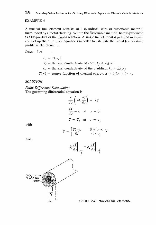
18 Boundary-Value Problems for Ordinary Differential Equations: Discrete Variable Methods
EXAMPLE 4
A nuclear fuel element consists of a cylindrical core of fissionable materialsurrounded by a metal cladding. Within the fissionable material heat is producedas a by-product of the fission reaction. A single fuel element is pictured in Figure2.2. Set up the difference equations in order to calculate the radial temperatureprofile in the element.
Data: Let
T( I'c)thermal conductivity of core, kf =1= ktC I')
thermal conductivity of the cladding, kc =1= kc ( I')
source function of thermal energy, S = 0 for I' > I'f
SOLUTION
Finite Difference FormulationThe governi~g differential equation is:
ddl
, ( I,k ~:) I'S
dT o at I' = 0dt<
withT= Tc at I' = I'c
S = {S(/'), 0,;;; I" ::::::; I'J
0, I' > I'J
and
COOLANT-<>CLADDING
CORE
A.c fiGURE 2.2 Nuclear fuel element.
Finite Difference Methods
By using (2.84), the difference formula becomes
k [Ui+l - Ui ] k [Ui - Ui - 1 ]- /0. 1 + /0. 1
1+ 2 hi 1-2 hi- 1
19
If i = °is the center point and i = j is the point /Of' then the system of differenceequations becomes
U 1 - Uo = °
i = 1, ... ,j-1
Nonlinear Second-Order Equations
We now consider finite difference methods for the solution of nonlinear boundary-value problems of the form
Ly(x) == - y" + f(x, y, y') = 0,
y(a) = Ct, y(b) = ~
a<x<b (2.89a)
(2.89b)
If a uniform mesh is used, then a second-order difference approximation to(2.89) is:
L = - [Ui + 1 - 2ui + Ui - 1 ] f (. . Ui+l - Ui - 1) = 0,hUi - h2 + X" u" 2h
i = 1,2, ... , N (2.90)
Uo = Ct,
The resulting difference equations (2.90) are in general nonlinear, and we shalluse Newton's method to solve them (see Appendix B). We first write (2.90) inthe form
<I'(u) = 0 (2.91)
80 Boundary-Value Problems for Ordinary Differential Equations: Discrete Variable Methods
where
and
h2
<p.(U) = - L u·I 2 h I
The Jacobian of «P(u) is the tridiagonal matrix
°J(U) = a«p(u) =
au
°where
(2.92)
i = 1,2, ... ,N
1 [ h at ( U i + l - U i - l )]A;(u) = - 2: 1 + "2 ay' Xi' Ui, 2h '
Bi(u) = [1 + ~2 :~ (Xi' Ui, Ui+l ~ U;-l)1C;(u) = - ~ [1 - ~ :: (Xi' Ui, U;+l ~ Ui-l)1
and
i = 2,3, ... ,N
i = 1,2, ... , N - 1
with
at ( Ui+l - U;-l) l'Say' Xi' Ui' 2h
at ( ')ay' Xi' y, Y
and
y evaluated by U i
y' evaluated by Ui + l ~ U
i-
l
In computing <Pl(u), <PN(u), AN(u), Bl(u), BN(u), and Cl(U), we use Uo = exand UN+l = 13. Now, with any initial estimate u[O] of the quantities U;,i = 1, 2 . . . , N, we define
U[k+l] = U[k] + AU[k],
where AU[k] is the solution of
k = 0,1,2, ...
k = 0,1,2, ...
(2.93)
(2.94)
Finite Difference Methods 81
More general boundary conditions than those in (2.89b) are easily incorporatedinto the difference scheme.
EXAMPLE 5
A class of problems concerning diffusion of oxygen into a cell in which anenzyme-catalyzed reaction occurs has been formulated and studied by means ofsingular perturbation theory by Murray [7]. The transport equation governingthe steady concentration C of some substrate in an enzyme-catalyzed reactionhas the general form
'i/(D'i/C) = g(C)
Here D is the molecular diffusion coefficient of the substrate in the mediumcontaining uniformly distributed bacteria and g(C) is proportional to the reactionrate. We consider the case with constant diffusion coefficient Do in a sphericalcell with a Michaelis-Menten theory reaction rate. In dimensionless variablesthe diffusion kinetics equation can now be written as
where
O<x<l
rx=
R'( )
_ C(r)y x - Co' = (DoCO
)8 R 2 'nq
_ -1 y(x)f(y) - 8 y(x) + k'
k=km
Co
Here R is the radius of the cell, Co is the constant concentration of the substratein r > R, km is the Michaelis constant, q is the maximum rate at which each cellcan operate, and n is the number of cells.
Assuming the cell membrane to have infinite permeability, it follows that
y(l) = 1
Further, from the assumed continuity and symmetry of y(x) with respect tox = 0, we must have
y'(O) = 0
There is no closed-form analytical solution to this problem. Thus, solve thisproblem using a finite difference method.
SOLUTION
The governing equation is
2or y" + - y' - f(y) = 0
x
82 Boundary-Value Problems for Ordinary Differential Equations: Discrete Variable Methods
with y(l) = 1 and y'(O) = O. With the mesh spacing h = lI(N + 1) and meshpoint Xi = ih,
i = 1,2, ... , N
with U N + 1 = 1.0. For X = 0, the second term in the differential equation isevaluated using L'Hospital's rule:
. (y') y"LIm - =-x->o X 1
Therefore, the differential equation becomes
3y" - fey) = 0
at x = 0, for which the corresponding difference replacement is
h2
U1 - 2uo + U- 1 - 3 f(uo) = 0
Using the boundary condition y' (0) = 0 gives
h2
U 1 - Uo - (; f(uo) = 0
The vector <I»(u) becomes
and the Jacobian is
J(u)
Finite Difference Methods
where
hZ k)+ - X ----:c
6£ (uo + k)Z
83
(2.95a)
(2.95b)
Ai = (1 - ~), l = 1,2, ... , N
Bi = - (2 + ~z x (ui~ k)Z), i = 1,2, ... , N
Ci=(l+~), i=1,2, ... ,N-i
Therefore, the matrix equation (2.94) for this problem involves a tridiagonallinear system of order N + 1.
The numerical results are shown in Table 2.4. For increasing values of N,the approximate solution appears to be converging to a solution. Decreasing thevalue of TOL below 10-6 gave the same results as shown in Table 2.4; thus thedifferences in the solutions presented are due to the error in the finite differenceapproximations. These results are consistent with those presented in Chapter 6of [1].
The results shown in Table 2.4 are easy to interpret from a physical standpoint. Since y represents the dimensionless concentration of a substrate, andsince the substrate is consumed by the cell, the value of y can never be negativeand should decrease as x decreases (moving from the surface to the center ofthe cell).
flrst·Order Systems
In this section we shall consider the general systems of m first-order equationssubject to linear two-point boundary conditions:
Ly = y' - f(x, y) = 0, a < x < b
Ay(a) + By(b) = a
TABLE 1.4 Results of Example 5, TOt = (- 6) on Newton Iteration, E = 0.1,k = 0.1
x
0.00.20.40.60.81.0
N=5
0.283( -1)0.430( -1)0.1030.2590.5531.000
N = 100.243( -1)0.384( -1)0.998( -1)0.2570.5521.000
N = 20
0.232( -1)0.372( -1)0.989(-1)0.2570.5521.000
N = 40
0.229( -1)0.369( -1)0.987( -1)0.2570.5521.000
N = 80
0.228( -1)0.368( -1)0.987( -1)0.2570.5521.000
84 Boundary-Value Problems for Ordinary Differential Equations: Discrete Variable Methods
As before, we take the mesh points on [a, b] as
Xi = a + ih,
b - ah=-
N+1
i = 0, 1, ... , N + 1 (2.96)
Let the m-dimensional vector U i approximate the solution y(xJ , and approximate(2.95a) by the system of difference equations
L - Ui - Ui - l f ( Ui + U i - l ) = 0,hUi - h - X i -1/2, 2
i = 1,2, ... , N + 1
The boundary conditions are given by
Auo + BUN + I - 01. = 0
(2.97a)
(2.97b)
The scheme (2.97) is known as the centered-difference method. The nonlinearterm in (2.95a) might have been chosen as
~ [f(x i, ui ) + f(xi-I> Ui - l )]
resulting in the trapezoidal rule.On defining the meN + 2)-dimensional vector U by
(2.97) can be written as the system of meN + 2) equations
Auo + BUN + I - 01.
hLhu I
(2.98)
(2.99)
<I>(U) = 0 (2.100)
(2.102)
With some initial guess, UfO], we now compute the sequence of U[kl's by
U[k+l] = U[k] + aU[k1, k = 0, 1,2, . . . (2.101)
where aU[kl is the solution of the linear algebraic system
a<I>(U[k1) aU[kl = _ <I>(U[k1)au
One of the advantages of writing a BVP as a first-order system is thatvariable mesh spacings can be used easily. Let
a = Xo < Xl < ... < XN+I = b (2.103)
h = max hi
Finite Difference Methods 85
be a general partition of the interval [a, b].The approximation for (2.95) using (2.103) with the trapezoidal rule is
(2.104)
where
h;-lLh"; = "; - ";-1 - hi;l [f(x;, "i) + f(xi_v ";-1)], i = 1, ... , N + 1
By allowing the mesh to be graded in the region of a sharp gradient, nonuniformmeshes can be helpful in solving problems that possess solutions or derivativesthat have sharp gradients.
Higher-Order Methods
The difference scheme (2.63) yields an approximation to the solution of (2.52)with an error that is 0(h2 ). We shall briefly examine two ways in which, withadditional calculations, difference schemes may yield higher-order approximations. These error-reduction procedures are Richardson's extrapolation and deferred corrections.
The basis of Richardson's extrapolation is that the error E;, which is thedifference between the approximation and the true solution, can be written as
(2.105)
(2.106)
where the functions a/x;) are independent of h. To implement the method, onesolves the BVP using successively smaller mesh sizes such that the larger meshesare subsets of the finer ones. For example, solve the BVP twice, with mesh sizesof hand h12. Let the respective solutions be denoted ulh) and ulhI2). For anypoint common to both meshes, x; = ih = 2i(hI2) ,
y(x;) - ui(h) = h2a1(x;) + h4a2(x;) + .
y(x;) - U i (~) = ~ a1(x;) + ~~ a2(x;) + .
Eliminate a1(x;) from (2.106) to give
(2.107)
Thus an 0(h4) approximation to y(x) on the mesh with spacing h is given by
u· = i u. (~)I 3 I 2 i = 0, 1, ... , N + 1 (2.108)
86 Boundary-Value Problems for Ordinary Differential Equations: Discrete Variable Methods
A further mesh subdivision can be used to produce a solution with error 0(h6),
and so on.For some problems Richardson's extrapolation is useful, but in general,
the method of deferred corrections, which is described next, has proven to besomewhat superior [8].
The method of deferred corrections was introduced by Fox [9], and hassince been modified and extended by Pereyra [10-12]. Here, we will outlinePereyra's method since it is used in software described in the next section.
Pereyra requires the BVP to be in the following form:
y' = f(x, y), a < x < b
g(y(a), y(b)) = 0
and uses the trapezoidal rule approximation
Ui+1 - U; - ~ h [f(x;, u;) + f(Xi+1' U;+l)] = hT(u;+1/2)
(2.109)
(2.110)
where T(U;+1/2) is the truncation error. Next, Pereyra writes the truncation errorin terms of higher-order derivatives
o
q
T(U;+1/2) = - L [ash2Sf}~si/2] + 0(h2s +2)s~l
where
s
22S - 1 (2s + 1)(2s!)
q number of terms in series (sets the desired accuracy)
The first approximation ul1] is obtained by solving
ul~l - ul1] - ~ h[f(x;, ul1
]) + f(x;+v ul~l)]
i = 0, 1, ... , N
g(U[l] U[l] ) = 00' N+1
(2.111)
(2.112)
where the truncation error is ignored. This approximation differs from the truesolution by 0(h2
).
The process proceeds as follows. An approximate solution U[k] [differs fromthe true solution by terms of order 0(h2k)] can be obtained from:
ul~l - ulkJ ~ h [f(x;, ulk]) + f(x;+1J ul~l)] = hT[k-1](ul:~/~)
i = 0,1, ... ,N
g(U[k] U[k] ) = 0)0' N+1
(2.113)
Mathematical Software
where
87
T[k-l] = T with q = k -1
In each step of (2.113), the nonlinear algebraic equations are solved by Newton'smethod with a convergence tolerance ofless than O(h2k). Therefore, using (2.112)gives uP] (O(h2)), which can be used in (2.113) to give U~2] (O(h4)). Successiveiterations of (2.113) with increasing k can give even higher-order accurate approximations.
MATHEMATICAL SOFTWARE
The available software that is based on the methods of this chapter is not asextensive as in the case of IVPs. A subroutine for solving a BVP will be designedin a manner similar to that outlined for IVPs in Chapter 1 except for the factthat the routines are much more specialized because of the complexity of solvingBVPs. The software discussed below requires the BVPs to be posed as firstorder systems (usually allows for simpler algorithms). A typical calling sequencecould be
CAll DRIVE (FUNC, DFUNC, BOUND, A, B, U, Tal)
where
FUNC = user-written subroutine for evaluating rex, y)
DFUNC = user-written subroutine for evaluating the Jacobian of rex, y)
BOUND = user-written subroutine for evaluating the boundary conditions and,if necessary, the Jacobian of the boundary conditions
A = left boundary point
B = right boundary point
U = on input contains initial guess of solution vector, and on outputcontains the approximate solution
TaL = an error tolerance
This is a simplified calling sequence, and more elaborate ones are actually usedin commercial routines.
The subroutine DRIVE must contain algorithms that:
1. Implement the numerical technique
2. Adapt the mesh-size (or redistribute the mesh spacing in the case of nonuniform meshes)
3. Calculate the error so to implement step (2) such that the error does notsurpass TaL
88 Boundary-Value Problems for Ordinary Differential Equations: Discrete Variable Methods
Implicit within these steps are the subtleties involved in executing the varioustechniques, e.g., the position of the orthonormalization points when using superposition.
Each of the major mathematical software libraries-IMSL, NAG, andHARWELL--eontains routines for solving BVPs. IMSL contains a shootingroutine and a modified version of DD04AD (to be described below) that usesa variable-order finite difference method combined with deferred corrections.HARWELL possesses a multiple shooting code and DD04AD. The NAG libraryincludes various shooting codes and also contains a modified version of DD04AD.Software other than that of IMSL, HARWELL, and NAG that is available islisted in Table 2.5. From this table and the routines given in the main libraries,one can see that the software for solving BVPs uses the techniques that areoutlined in this chapter.
We illustrate the use of BVP software packages by solving a fluid mechanicsproblem. The following codes were used in this study:
1. HARWELL, DD03AD (multiple shooting)
2. HARWELL, DD04AD
Notice we have chosen a shooting and a finite difference code. The third majormethod, superposition, was not used in this study. The example problem isnonlinear and would thus require the use of SUPORQ if superposition is to beincluded in this study. At the time of this writing SUPORQ is difficult to implement and requires intimate knowledge of the code for effective utilization.Therefore, it was excluded from this study. DD03AD and DD04AD will nowbe described in more detail.
DD03An [18]
This program is the multiple-shooting code of the Harwell library. In this algorithm, the interval is subdivided and "shooting" occurs in both directions.The boundary-value problem must be specified as an initial-value problem withthe code or the user supplying the initial conditions. Also, the partitioning ofthe interval can be user-supplied or performed by the code. A tolerance parameter (TOL) controls the accuracy in meeting the continuity conditions at the
TABLE 2.5 BVP Codes
Name
BOUNDSSHOOTlSHOOT2MSHOOTSUPORTSUPORQ
Method Implemented
Multiple shootingShooting with separated boundary conditionsSame as SHOOTI with more general boundary conditionsMutliple shootingSuperposition (linear problems only)Superposition with quasilinearization
Reference
[13,14][15][15][15][4][16]
Mathematical Software 89
matching points [see (2.35)]. This type of code takes advantage of the highlydeveloped software available for IVPs (uses a fourth-order Runge-Kutta algorithm [19]).
DD04AD [.7, 20]
This code was written by Lentini and Fe~eyra and is described in detail in [20].Also, an earlier version of the code is discussed in [17]. The code implementsthe trapezoidal approximation, and the resulting algebraic system is solved bya modified Newton method. The user is permitted to specify an initial intervalpartition (which does not need to be uniform), or the code.provides a coarse,equispaced one. The user may also specify an initial estimate for the solution(the default being zero). Deferred corrections is used to increase accuracy andto calculate error estimates. An error tolerance (TOL) is provided by the user.Additional mesh points are automatically added to the initial partition with theaim of reducing error to the user-specified level, and also with the aim of equidistribution of error throughout the interval [17]. The new mesh points are alwaysadded between the existing mesh points. For example, if xj and xj + 1 are initialmesh points, then if m mesh points t;, i = 1, 2, ... , m, are required to beinserted into [Xj' Xj + 1], they are placed such that
(2.114)
(2.116)
where
t2 - xj t;+1 t;-1 Xj+1 - tm - 1t1 = --2-' ... , t; = --2--' ... , tm = --'----2--
The approximate solution is given as a discrete function at the points of the finalmesh.
Example Problem
The following BVP arises in the study of the behavior of a thin sheet of viscousliquid emerging from a slot at the base of a converging channel in connectionwith a method of lacquer application known as "curtain coating" [21]:
d2y _ ! (dy )2 _ ydy + 1 = 0 (2.115)
dx2 Y dx dx
The function y is the dimensionless velocity of the sheet, and x is the dimensionless distance from the slot. Appropriate boundary conditions are [22]:
y = Yo at x = 0
dy ---7 (2X)-1/2 at sufficiently large xdx
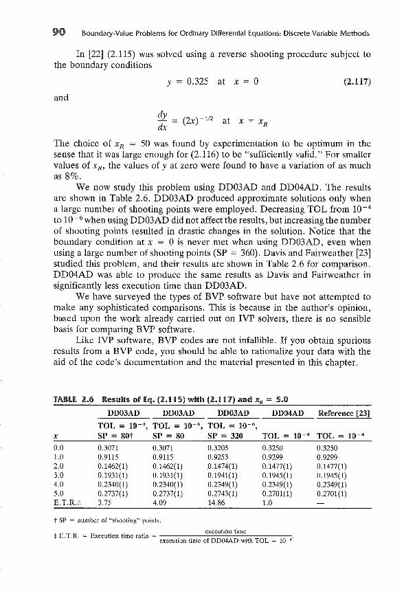
90 Boundary-Value Problems for Ordinary Differential Equations: Discrete Variable Methods
In [22] (2.115) was solved using a reverse shooting procedure subject tothe boundary conditions
and
y = 0.325 at x = 0 (2.117)
dy = (2X)-1/2 at x = xdx R
The choice of XR = 50 was found by experimentation to be optimum in thesense that it was large enough for (2.116) to be "sufficiently valid." For smallervalues of XR, the values of y at zero were found to have a variation of as muchas 8%.
We now study this problem using DD03AD and DD04AD. The resultsare shown in Table 2.6. DD03AD produced approximate solutions only whena large number of shooting points were employed. Decreasing TOL from 10-4
to 10 -6 when using DD03AD did not affect the results, but increasing the numberof shooting points resulted in drastic changes in the solution. Notice that theboundary condition at x = 0 is never met when using DD03AD, even whenusing a large number of shooting points (SP = 360). Davis and Fairweather [23]studied this problem, and their results are shown in Table 2.6 for comparison.DD04AD was able to produce the same results as Davis and Fairweather insignificantly less execution time than DD03AD.
We have surveyed the types of BVP software but have not attempted tomake any sophisticated comparisons. This is because in the author's opinion,based upon the work already carried out on IVP solvers, there is no sensiblebasis for comparing BVP software.
Like IVP software, BVP codes are not infallible. If you obtain spuriousresults from a BVP code, you should be able to rationalize your data with theaid of the code's documentation and the material presented in this chapter.
TABLE 2.6 Results of Eq. (2.1' 5) with (2.117) and X R = 5.0
DD03AD DD03AD DD03AD DD04AD Reference [23]
x
0.01.02.03.04.05.0E.T.R.*
TOL = 10-4,SP = SOt
0.30710.91150.1462(1)0.1931(1)0.2340(1)0.2737(1)3.75
TOL = 10- 6 ,
SP = SO
0.30710.91150.1462(1)0.1931(1)0.2340(1)0.2737(1)4.09
TOL = 10-6 ,
SP = 3200.32050.92530.1474(1)0.1941(1)0.2349(1)0.2743(1)14.86
TOL = 10-4
0.32500.92990.1477(1)0.1945(1)0.2349(1)0.2701(1)1.0
TOL = 10-4
0.32500.92990.1477(1)0.1945(1)0.2349(1)0.2701(1)
t SP = number of "shooting" points.
+E.T.R. = Execution time ratioexecution time
execution time of DD04AD with TOL = 10-4'
Problems
1. Consider the BVP
PROBLEMS
y" + r(x)y = f(x),
yea) = a
y(b) = f3
a<x<b
91
Show that for a uniform mesh, the integration method gives the sameresult as Eq. (2.64).
2. Refer to Example 4. If
S(r) = So[ 1 + b (;~r]solve the governing differential equation to obtain the temperature profilein the core and the cladding. Compare your results with the analyticalsolution given on page 304 of [24]. Let kc = 0.64 cal/(s·cm·K), kf = 0.066cal/(s·cm·K), To = 500 K, I'-c = ~ in, and I"f = ~ in.
3.* Axial conduction and diffusion in an adiabatic tubular reactor can bedescribed by [2]:
1 d 2C dC- - - - - R(C T) = 0Pe dx2 dx '
1 d 2T dT- -- - - - f3R (C T) = 0Bo dx2 dx '
with
and
1 dCPe -dx = C- 1}1 dT-- = T - 1
Bo dx
at x= 0
dC = O}:~ = 0 at x = 0
dx
Calculate the dimensionless concentration C and temperature T profiles forf3 = -0.05,Pe = Bo = 10,E = 18,andR(C, T) = 4Cexp[E(1-l/T)].
4.* Refer to Example 5. In many reactions the diffusion coefficient is a function
o at x = 0
92 Boundary-Value Problems for Ordinary Differential Equations: Discrete Variable Methods
of the substrate concentration. The diffusion coefficient can be of form[1]:
D(y) = 1 + A-Do (y + kz)Z
Computations are of interest for A- = kz = lO-z, with e and k as in Example5. Solve the transport equation using D(y) instead of D for the parameterchoice stated above. Next, let A- = 0 and show that your results comparewith those of Table 2.4.
S.* The reactivity behavior of porous catalyst particles subject to both internalmass concentration gradients as well as temperature gradients can be studied with the aid of the following material and energy balances:
dZy + ~ dy = <pZyexp ['Y (1 _1.)]dxz xdx T
~:~ + ~ ~~ = - ~<pZy exp [ 'Y (1 - ~)]with
dT = dy = 0 at x = 0dx dx
T = y = 1 at x = 1
where
y = dimensionless concentration
T = dimensionless temperature
x = dimensionless radial coordiante (spherical geometry)
<p = Thiele modulus (first-order reaction rate)
'Y = Arrhenius number
~ = Prater number
These equations can be combined into a single equation such that
dZy + ~ dy = <pz ex [ 'Y~(1 - y) ]dxz x dx Y P 1 + ~(1 - y)
with
dydx
y = 1 at x = 1
For 'Y 30, ~ 0.4, and <p = 0.3, Weisz and Hicks [25] found three
References 93
solutions to the above equation using a shooting method. Calculate thedimensionless concentration and temperature profiles of the three solutions.
Hint: Try various initial guesses.
REfERENCES
1. Keller, H. B., Numerical Methods for Two-Point Boundary-Value Problems, Blaisdell, New York (1968).
2. Carberry, J. J., Chemical and Catalytic Reaction Engineering, McGrawHill, New York (1976).
3. Deuflhard, P., "Recent Advances in Multiple Shooting Techniques," inComputational Techniques for Ordinary Differential Equations,!. Gladwelland D. K. Sayers (eds.), Academic, London (1980).
4. Scott, M. R., and H. A. Watts, SUPORT-A Computer Code for TwoPoint Boundary-Value Problems via Orthonormalization, SAND75-0198,Sandia Laboratories, Albuquerque, N. Mex. (1975).
5. Scott, M. R., and H. A. Watts, "Computational Solutions of Linear TwoPoint Boundary Value Problems via Orthonormalization," SIAM J. Numer. Anal., 14, 40 (1977).
6. Varga, R. S., Matrix Iterative Analysis, Prentice-Hall, Englewood Cliffs,N.J. (1962).
7. Murray, J. D., "A Simple Method for Obtaining Approximate Solutionsfor a Large Class of Diffusion-Kinetic Enzyme Problems," Math. Biosci.,2 (1968).
8. Fox, L., "Numerical Methods for Boundary-Value Problems," in Computational Techniques for Ordinary Differential Equations,!. Gladwell andD. K. Sayers (eds.), Academic, London (1980).
9. Fox, L., "Some Improvements in the Use of Relaxation Methods for theSolution of Ordinary and Partial Differential Equations," Proc. R. Soc.A, 190, 31 (1947).
10. Pereyra, V., "The Difference Correction Method for Non-Linear TwoPoint Boundary Problems of Class M," Rev. Union Mat. Argent. 22, 184(1965).
11. Pereyra, V., "High Order Finite Difference Solution of Differential Equations," STAN-CS-73-348, Computer Science Dept., Stanford Univ., Stanford, Calif. (1973).
12. Keller, H. B., and V. Pereyra, "Difference Methods and Deferred Corrections for Ordinary Boundary Value Problems," SIAM J. Numer. Anal.,16, 241 (1979).
94 Boundary-Value Problems for Ordinary Differential Equations: Discrete Variable Methods
13. Bulirsch, R., "Multiple Shooting Codes," in Codes for Boundary-ValueProblems in Ordinary Differential Equations, Lecture Notes in ComputerScience, 76, Springer-Verlag, Berlin (1979).
14. Deuflhard, P., "Nonlinear Equation Solvers in Boundary-Value Codes,"Rep. TUM-MATH-7812. Institut fur Mathematik, Universitat Munchen(1979).
15. Scott, M. R. and H. A. Watts, "A Systematized Collection of Codes forSolving Two-Point Boundary-Value Problems," Numerical Methods forDifferential Systems, L. Lapidus and W. E. Schiesser (eds.), Academic,New York (1976). .
16. Scott, M. R., and H. A. Watts, "Computational Solution of NonlinearTwo-Point Boundary Value Problems," Rep. SAND 77-0091, Sandia Laboratories, Albuquerque, N. Mex. (1977).
17. Lentini, M., and V. Pereyra, "An Adaptive Finite Difference Solver forNonlinear Two-Point Boundary Problems with Mild Boundary Layers,"SIAM J. Numer. Anal., 14, 91 (1977).
18. England, R., "A Program for the Solution of Boundary Value Problemsfor Systems of Ordinary Differential Equations," Culham Lab., Abingdon:Tech. Rep. CLM-PDM 3/73 (1976).
19. England, R., "Error Estimates for Runge-Kutta Type Solutions to Systemsof Ordinary Differential Equations," Comput. J., 12, 166 (1969).
20. Pereyra, V., "PASVA3-An Adaptive Finite-Difference FORTRAN Program for First-Order Nonlinear Ordinary Boundary Problems," in Codesfor Boundary-Value Problems in Ordinary Differential Equations, LectureNotes in Computer Science, 76, Springer-Verlag, Berlin (1979).
21. Brown, D. R., "A Study of the Behavior of a Thin Sheet of MovingLiquid," J. Fluid Mech., 10, 297 (1961).
22. Salariya, A. K., "Numerical Solution of a Differential Equation in FluidMechanics," Comput. Methods Appl. Mech. Eng., 21,211 (1980).
23. Davis, M., and G. Fairweather, "On the Use of Spline Collocation forBoundary Value Problems Arising in Chemical Engineering," Comput.Methods Appl. Mech. Eng., 28, 179 (1981).
24. Bird, R. B., W. E. Stewart, and E. L. Lightfoot, Transport Phenomena,Wiley, New York (1960).
25. Weisz, P. B., and J. S. Hicks, "The Behavior of Porous Catalyst Particlesin View of Internal Mass and Heat Diffusion Effects," Chern. Eng. Sci.,17, 265 (1962).
Bibliography
BIBLIOGRAPHY
95
For additional or more detailed information concerning boundary-value problems, see thefollowing:
Aziz, A. Z. (ed.), Numerical Solutions of Boundary-Value Problems for Ordinary Differential Equations, Academic, New York (1975).
Childs, B., M. Scott, J. W. Daniel, E. Denman, and P. Nelson (eds.), Codes for Boundary-Value Problems in Ordinary Differential Equations, Lecture Notes in ComputerScience, Volume 76, Springer-Verlag, Berlin (1979).
Fox, L., The Numerical Solution of Two-Point Boundary-Value Problems in OrdinaryDifferential Equations, (1957).
Gladwell, 1., and D. K. Sayers (eds.), Computational Techniques for Ordinary DifferentialEquations, Academic, London (1980).
Isaacson, E., and H. B. Keller, Analysis ofNumerical Methods, Wiley, New York (1966).
Keller, H. B., Numerical Methods for Two-Point Boundary-Value Problems, Blaisdell,New York (1968).
Russell, R. D., Numerical Solution of Boundary Value Problems, Lecture Notes, Universidad Central de Venezuela, Publication 79-06, Caracas (1979).
Varga, R. S., Matrix Iterative Analysis, Prentice-Hall, Englewood Cliffs, N.J. (1962).
Boundary-Value ProblemsOrdinary Differential Equations:finite Element Methods
INTRODUCTION
The numerical techniques outlined in this chapter produce approximate solutionsthat, in contrast to those produced by finite difference methods, are continuousover the interval. The approximate solutions are piecewise polynomials, thusqualifying the techniques to be classified as finite element methods [1]. Here,we discuss two types of finite element methods: collocation and Galerkin.
BACKGROUND
Let us begin by illustrating finite elements methods with the following BVP:
y" = y + [(x),
yeO) = 0y(1) = 0
O<x<l (3.b)
(3.th)
Finite element methods find a piecewise polynomial (pp) approximation, u(x),to the solution of (3.1). A piecewise polynomial is a function defined on apartition such that on the subintervals defined by the partition, it is a polynomial.The pp-approximation can be represented by
m
u(x) = 2: aj<pj(x)j=l
(3.2)
97
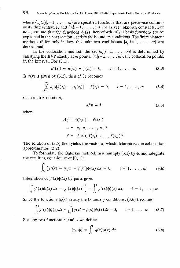
98 Boundary-Value Problems for Ordinary Differential Equations: Finite Element Methods
where {<!>Jx)lj= 1, ... , m} are specified functions that are piecewise continuously differentiable, and {ah =1, ... , m} are as yet unknown constants. Fornow, assume that the functions <!>j (x), henceforth called basis functions (to beexplained in the next section), satisfy the boundary conditions. The finite elementmethods differ only in how the unknown coefficients {ajlj= 1, ... , m} aredetermined.
In the collocation method, the set {ajU = 1, ... , m} is determined bysatisfying the BVP exactly at m points, {xiii = 1, ... ,m}, the collocation points,in the interval. For (3.1):
u"(xi) - u(x;) - f(xi) = 0,
If u(x) is given by (3.2), then (3.3) becomes
i = 1, ... ,m (3.3)
m
L aj[<!>j(xi) - <!>j(xi)] - f(xi) = 0,j=1
i = 1, ... ,m (3.4)
or in matrix notation,
(3.5)
where
(3.6)i = 1, ... ,m
The solution of (3.5) then yields the vector a, which determines the collocationapproximation (3.2).
To formulate the Galerkin method, first multiply (3.1) by <!>i and integratethe resulting equation over [0, 1]:
f [y"(x) - y(x) - f(X)]<!>i(X) dx = 0,
Integration of y"(x)<!>;(x) by parts gives
fa1
Y"(X)<j>i(X) dx = Y'(X)<!>i(X) I~ -f y' (x)<j>; (x) dx, i = 1, ... ,m
i=I, ... ,m
Since the functions <!>/x) satisfy the boundary conditions, (3.6) becomes
L1Y'(X)<!>;(X)dX +f [y(x) + f(X)J<l>i(X)dx = 0, (3.7)
For any two functions 'Y] and tjJ we define
('Y], tjJ) = f 'Y](x)tjJ(x) dx (3.8)
Piecewise Polynomial Functions
With (3.8), Eq. (3.7) becomes
(y', <pD + (y, <Pi) + (f, <PJ = 0, i = 1, ... ,m
99
(3.9)
and is called the weak form of (3.1). The Galerkin method consists of findingu(x) such that
i = 1, ... ,m(u ', <pD + (u, <Pi) + (f, <PJ = 0,
If u(x) is given by (3.2), then (3.10) becomes:
(i: aj<p;, <P:) + (i: aj<pj, <Pi) + (f, <Pi) = 0,J=l J=l
or, in matrix notation,
where
g = [11' ... ,JrnV1i = (f, <Pi)
i=l, ... ,m
(3.10)
(3.11)
(3.12)
The solution of (3.12) gives the vector a, which specifies the Galerkin approximation (3.2).
Before discussing these methods in further detail, we consider choices ofthe basis functions.
PIECEWISE POLYNOMIAL FUNCTIONS
To begin the discussion of pp-functions, let the interval partition 'IT be given by:
with
a = Xl < X2 < ... < Xe+1 = b
h = max hj = max (xj + 1 - XJ)l,;;;j,;;;e l,;;;j,;;;e
(3.13)
Also let {Pj(x)lj = 1, ... , €} be any sequence of € polynomials of order k(degree <:;; k - 1). The corresponding pp-function, F(x), of order k is definedby
(3.14)
j = 1, ... ,€
100 Boundary-Value Problems for Ordinary Differential Equations: Finite Element Methods
where xj are called the breakpoints of F. By convention
F(x) = {Pl(X),Pix),
and
(3.15)
F(xJ = Pi(x;) (right continuity) (3.16)
A portion of a pp-function is illustrated in Figure 3.1. The problem is how toconveniently represent the pp-function.
Let S be a set of functions:
S = {A./x)lj = 1, ... , L} (3.17)
The class of functions denoted by !ZJ is defined to be the set of all functionsf(x) of the form
L
f(x) = 2.: ajA.j(x)j=l
(3.18)
where the a/s are constants. This class of functions !ZJ defined by (3.18) is calleda linear function space. This is analogous to a linear vector space, for if vectorsxj are substituted for the functions A./x) in (3.18), we have the usual definitionof an element x of a vector space. If the functions A.j in S are linearly independent,then the set S is called a basis for the space !ZJ, L is the dimension of the space!ZJ, and each function A.j is called a basis function.
Define !ZJk (7I") (subspace of !ZJ) to be the set of all pp-functions of orderk on the partition 71". The dimension of this space is
(3.19)
Let v be a sequence of nonnegative integers vj, that is, v = {vjlj = 2, ... , e},such that
d i - l
jumpXj dX i - l [f(x)] = 0 (3.20)
i = 1, ... , Vj' j = 2, ... ,e
\rPj
\P j - I ~
~~
fiGURE 3. t Piecewise polynomial function.
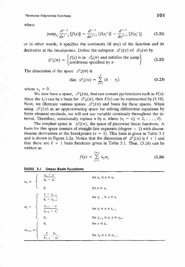
Piecewise Polynomial Functions
where
101
(3.21)
or in other words, 11 specifies the continuity (if any) of the function and its
derivative at the breakpoints. Define the subspace .0 k(1T) of .0k(1T) by
.0 v ( ) = {f(X) is in .0J1T) and satisfies the jump} (3.22)k 1T conditions specified by 11
The dimension of the space .0 kC1T) ise
dim .0 k(1T) ~ (k - vj )j=1
(3.23)
where VI = O.We now have a space, .0 k(1T), that can contain pp-functions such as F(x).
Since the 'A./s can be a basis for .0 k(1T), then F(x) can be represented by (3.18).Next, we illustrate various spaces .0k(1T) and bases for these spaces. Whenusing .0 k(1T) as an approximating space for solving differential equations byfinite element methods, we will not use variable continuity throughout the interval. Therefore, notationally replace 11 by v, where {vi = vlj = 2, ... , .e}.
The simplest space is .0i(1T), the space of piecewise linear functions. Abasis for this space consists of straight-line segments (degree = 1) with discontinuous derivatives at the breakpoints (v = 1). This basis is given in Table 3.1and is shown in Figure 3.2a. Notice that the dimension of .0 i(1T) is .e + 1 andthat there are .e + 1 basis functions given in Table 3.1. Thus, (3.18) can bewritten as
f(x)
TABU 3.t Linear Basis functions
(3.24)
0,
x - x j _ 1,xj - x j _ 1
0,
0,
x - X e ,X e+ 1 - X e
for x ;;. X2
for x'" Xe
forxe~X~Xe+l
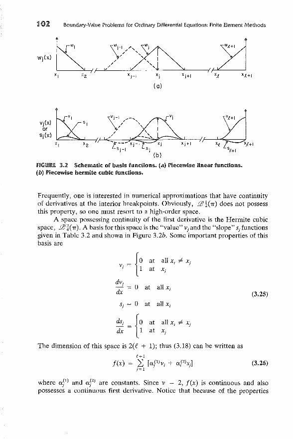
102 Boundary-Value Problems for Ordinary Differential Equations: Finite Element Methods
Wj(X)~ ~XI X2 Xj_1 Xj Xj+1 xl. x,( +1
(0)
~Vj(X) 51or
Sj(X)
XI X2 Xj+1 Xi
(b)
fiGURE 3.2 Schematic of basis fll.mctions. (a) Piecewise linear functions.(b) Piecewise hermite cubic functions.
Frequently, one is interested in numerical approximations that have continuityof derivatives at the interior breakpoints. Obviously, .Q? H'IT) does not possessthis property, so one must resort to a high-order space.
A space possessing continuity of the first derivative is the Hermite cubicspace, .Q? ~('IT). A basis for this space is the "value" vj and the "slope" Sj functionsgiven in Table 3.2 and shown in Figure 3.2b. Some important properties of thisbasis are
o at all Xi
(3.25)
Sj = 0 at all Xi
~>{~ at all Xi of- X jat x j
The dimension of this space is 2(.£ + 1); thus (3.18) can be written as
€+1
f(x) = ~ [ap)vj + aF)sj]j=1
(3.26)
where ay) and ay) are constants. Since v = 2, f(x) is continuous and alsopossesses a continuous first derivative. Notice that because of the properties
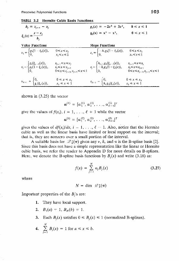
Piecewise Polynomial Functions
TABLE 3.2 Hermite Cubic Basis functions
103
hj = Xj + 1 - Xj gl(X) = -2x3 + 3x 2, O~x~l
x-x· g2(X) = X3- X2, O~x~l
~j(x)=TJ
Value Functions Slope Functions
VI = {gl(1 - ~1(X)), 0~X~X2 _ { -h1g2(1 - ~1(X», 0~X~X2
0, x2~x~1SI - 0,
x2~x~1
el(~j-'(X))' Xj _ 1 ::S;X:S;;Xj rj-lgO<~j-l(X»' Xj_l~X~Xj
Vj = gl(l-~j(x», XjS;;X:'!SXj + 1 Sj = - hjg2(1- Ux», Xj~X~Xj+l
0, O~X~Xj_l,Xj+l ~x~ 1 0, O~X~Xj_l,Xj+l ~x~l
{O, °~ x ~ xe {0, °~ x ~ xeVe+1 = gl(~e(X», xe ~ X ~ 1 se+l = hegi~eCx», xe ~ x ~ 1
shown in (3.25) the vector
(1) _ [(1) (1) (1) ]T01. - (Xl ,(X2 , ... , (Xe+l
give the values of f(x;), i = 1, ... , e + 1 while the vector
(2) _ [(2) (2) (2) ]T01. - (Xl '(X2 , .•• , (Xe+l
gives the values of df(x;)/dx, i = 1, ... , .e + 1. Also, notice that the Hermitecubic as well as the linear basis have limited or local support on the interval;that is, they are nonzero over a small portion of the interval.
A suitable basis for it k(1T) given any v, k, and 1T is the B-spline basis [2].Since this basis does not have a simple representation like the linear or Hermitecubic basis, we refer the reader to Appendix D for more details on B-splines.Here, we denote the B-spline basis functions by B/x) and write (3.18) as:
N
f(x) = ~ (XjBj(x)j=l
where
N = dim itk(1T)
Important properties of the B/s are:
1. They have local support.
2. Bl(a) = 1, BN(b) = 1.
3. Each B/x) satisfies 0 ~ Bj(x) ~ 1 (normalized B-splines).
N
4. ~ B/x) = 1 for a ~ x ~ b.j=l
(3.27)
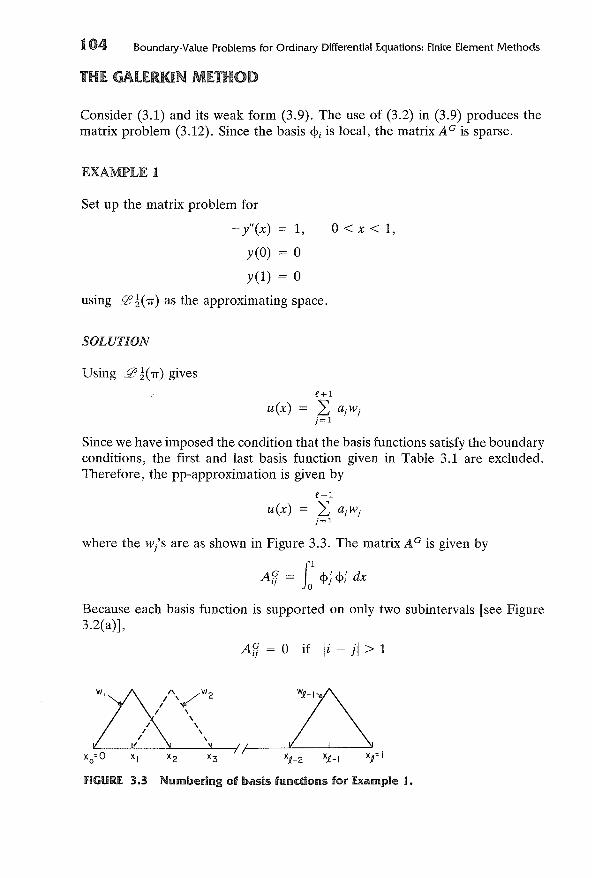
.04 Boundary-Value Problems for Ordinary Differential Equations: Finite Element Methods
THE GALERKIN METHOD
Consider (3.1) and its weak form (3.9). The use of (3.2) in (3.9) produces thematrix problem (3.12). Since the basis <l>i is local, the matrix A G is sparse.
EXAMPLE 1
Set up the matrix problem for
_y"(X) = 1,
yeO) = 0
y(l) = 0
using ..0 i (rr) as the approximating space.
SOLUTION
Using ..0i(-rr) gives
0< x < 1,
£+1
u(x) = L ajwjj=1
Since we have imposed the condition that the basis functions satisfy the boundaryconditions, the first and last basis function given in Table 3.1 are excluded.Therefore, the pp-approximation is given by
£-1
u(x) = L ajwjj= 1
where the w/s are as shown in Figure 3.3. The matrix AG is given by
A~ = r<1>;<1>: dx
Because each basis function is supported on only two subintervals [see Figure3.2(a)],
A~ = 0 if Ii - jl > 1
FIGURE 3.3 Numbering of basis functions for Example t.
Piecewise Polynomial Functions
Thus, A G is tridiagonal and
fXi [ 1 ]2 fXi+1 [ -1 ]2
= dx+ dxXi-l Xi - Xi- 1 Xi Xi+ 1 - Xi
1 1= - +-- hi = Xi - Xi- 1
hi hi+/
e (Xi+l [ -1 ] [ 1 ]A5+1 = J( <fJ;<fJ;+l dx = L _ _ dx
o x, Xi+l Xi Xi+1 Xi
1
G _ 1A i,i-l - - h-
I
The vector g is given by
Therefore, the matrix problem is:
105
o~ (hI + h2 )
! (h 2 + h3 )
1
he- 2ae- 2
1
(h:_J~(he-2 + he-I)
0 he- 2ae- 1
From Example 1, one can see that if a uniform mesh is specified using!l? ~ ('IT), the standard second-order correct finite difference method is obtained.
Therefore, the method would be second-order accurate. In general, the Galerkinmethod using !l?k('IT) gives an error such that [1]:
Ily - ull ~ Chk (3.28)
• 06 Boundary-Value Problems for Ordinary Differential Equations: Finite Element Methods
where
y = true solution
u = pp-approximation
C = a constant
h = uniform partition
IIQII = max IQIx
provided that y is sufficently smooth. Obviously, one can increase the accuracyby choosing the approximating space to be of higher order.
EXAMPLE 2
An insulated metal rod is exposed at each end to a temperature, To. Within therod, heat is generated according to the following function:
H(T - To) + cosh(1)]
where
~ = constant
T = absolute temperature
The rod is illustrated in Figure 3.4. The temperature profile in the rod can becalculated by solving the following energy balance:
d 2 TH(T - To) + cosh(1)]K dz2 =
T= To at z = 0
T= To at z = L
(3.29)
where K is the thermal conductivity of the metal. When (~L2)/K = 4, the solutionof the BVP is
y = cosh (2x - 1) - cosh (1)
where y = T - To and x = z/L. Solve (3.29) using the Hermite cubic basis,and show that the order of accuracy is O(h4) (as expected from 3.28).
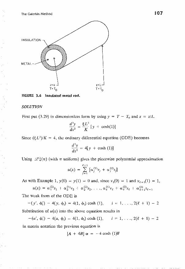
The Galerkin Method
INSULATION
METAL
fiGURE. 3.4 Insulated metal rod.
SOLUTION
z=LT=To
107
First put (3.29) in dimensionless form by using y = T - To and x = zlL.
d2 ~U~2 = - [y + cosh(1)]dx K
Since (~U)IK = 4, the ordinary differential equation (ODE) becomes
d 2ydx2 = 4[y + cosh (1)]
Using iZ'HTI) (with TI uniform) gives the piecewise polynomial approximation
e+1u(x) = 2: [aYlvj + a?lsJ
j~l
As with Example 1, y(O) = y(1) = 0 and, since v1(O) = 1 and ve+1(1) = 1,
u(x) = ai2ls1 + a~llv2 + a~2ls2' ... , a~llve + a~2lse + a~2l1se+1
The weak from of the ODE is
- (y', <p;) - 4(y, <PJ = 4(1, <Pi) cosh (1), i = 1, ... ,2(£ + 1) - 2
Substitution of u(x) into the above equation results in
- (u', <p;) - 4(u, <Pi) = 4(1, <Pi) cosh (1), i = 1, ... ,2(£ + 1) - 2
In matrix notation the previous equation is
[A + 4B] a = -4 cosh (1)F
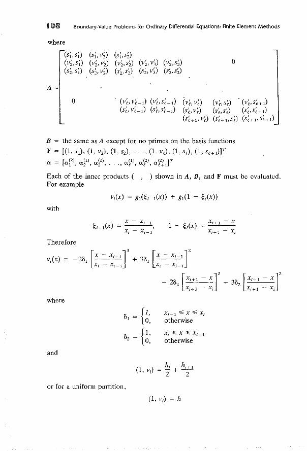
.08 Boundary-Value Problems for Ordinary Differential Equations: Finite Element Methods
where
(s~,sD (s~, v~) (s~,s~)
(v~, sD (v~, v~) (v~, s~) (v~, v~) (v~, sD(s~, sD (s~, vD (s~, s~) (s~, v;) (s;, s~)
A=
°
° (v~, V~-1) (V~,S~_1)
(s~, V~-1) (S~,S~_1)
(v~,v~)
(s~, v~)
(s~+l> v~)
(v~,s~) . (V~,S~+1)(s~, s~) (s~, s~ + 1)(s~+l>S~) (s~+l>S~+1)
B = the same as A except for no primes on the basis functions
F = [(1, S1), (1, v2), (1, S2), ... , (1, ve), (1, se), (1, Se+1)YOl = [a(2) a(1) a(2) a(1) a(2) a(2) ]T
1 , 2' 2'···' e, e, e+1
Each of the inner products ( , ) shown in A, B, and F must be evaluated.For example
with
x - X i - 1
Xi - X i - 1 '1 - ~;(x)
X i + 1 - X
Xi+1 - Xi
where
°1 = e' Xi-1 ~ X ~ Xi
0, otherwise
°2 ={I, Xi ~ X ~ X i + 1
0, otherwise
and
or for a uniform partition,
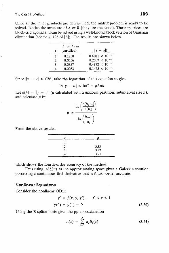
The Galerkin Method 109
Once all the inner products are determined, the matrix problem is ready to besolved. Notice the structure of A or B (they are the same). These matrices areblock-tridiagonal and can be solved using a well-known block version of Gaussianelimination (see page 196 of [3]). The results are shown below.
h (uniformpartition) tly - uti
1 0.1250 0.6011 x 10⁻⁵
2 0.0556 0.2707 x 10- 6
3 0.0357 0.4872 x 10⁻⁷
4 0.0263 0.1475 x 10⁻⁷
Since Ily - ull ~ ChP , take the logarithm of this equation to give
lnlly - ull ~ InC + pLnh
Let e(h) = Ily - ull (u calculated with a uniform partition; subinterval size h),and calculate p by
In (e(ht _ 1))
e(ht )
p = -----
In (h~~l)
From the above results,
p
1234
3.833.873.91
which shows the fourth-order accuracy of the method.Thus using .CZ? H1T) as the approximating space gives a Galerkin solution
possessing a continuous first derivative that is fourth-order accurate.
Nonlinear Equations
Consider the nonlinear ODE:
y" = f(x, y, y'),
y(O) = y(l) = 0
O<x<l
(3.30)
Using the B-spline basis gives the pp-approximation
N
u(x) = 2: ujBj(x)j~l
(3.31)
• • 0 Boundary-Value Problems for Ordinary Differential Equations: Finite Element Methods
Substitution of (3.31) into the weak form of (3.30) yields
(£OljBl, B;) + (t(x, £OljBj, £OljBl), B;) = 0,~1 J=l J=l
i = 1, ... ,N
The system (3.32) can be written as
A« + H(<<) = 0
(3.32)
(3.33)
where the vector H contains inner products that are nonlinear functions of «.Equation (3.33) can be solved using Newton's method, but notice that the vectorH must be recomputed after each iteration. Therefore, the computation of Hmust be done efficiently. Normally, the integrals in H do not have closed form,and one must resort to numerical quadrature. The rule of thumb in this case isto use at least an equal number of quadrature points as the degree of theapproximating space.
Inhomogeneous Dirichlet and Flux Boundary Conditions
The Galerkin procedures discussed in the previous sections may easily be modified to treat boundary conditions other than the homogeneous Dirichlet conditions, that is, yeO) = y(l) = O. Suppose that the governing ODE is
(a(x)y'(x))' + b(x)y(x) + c(x) = 0, 0 < x < 1 (3.34)
subject to the boundary conditions
y(l) = \j!2 (3.35)
where \j!1 and \j!2 are constants. The weak form of (3.34) is
Since
a(x)y' (x)B;(x)
o
(a(x)y' (x), B; (x)) + (b(x)y(x), B;(x))
+ (c(x), B;(x)) = 0 (3.36)
and
then
1,
N
2: Bj(O) = 0j~2
N-1
2: Bj (l) = 0j=l
(3.37)
The Galerkin Method 111
to match the boundary conditions. The value of i in (3.36) goes from 2 to N - 1so that the basis functions satisfy the homogeneous Dirichlet conditions [eliminates the first term in (3.36)]. Thus (3.36) becomes:
N-1
~ aj[(a(x)Bj, BD - (b(x)Bj, Bi)] = (c(x), Bi)j=2
+ t!J1[-(a(x)B~, BD + (b(x)Bv Bi )]
+ t!J2[ -(a(x)B~, BD + (b(x)BN> Bi )], i = 2, ... ,N - 1 (3.38)
If flux conditions are prescribed, they can be represented by
ThY + 131Y' ="'11 at x = 0
1llY + 132Y' ="'12 at x = 1
where 1]1> 1]2' 131, 132, "'11' and "'12 are constants and satisfy
h11 + 11311 > 0
11]21 + 11321 > 0Write (3.39) as
"'11 1]1y' = - - - Y at x = 0131 131
(3.39)
"'12 1]2y' = - - - Y at x = 1 (3.40)132 132
Incorporation of (3.40) into (3.36) gives:
f uj[(a(X)Bj, BD - (b(x)Bj, Bi ) - OnOj1a(0) 1]1 + oiNojN a(l) 1]2]j=l 131 132
where
i = 1, ... ,N (3.41)
{
I,Os, =
0,
s = t
s -# t
Notice that the subscript i now goes from 1 to N, since yeO) and y(l) areunknowns.
Mathematical Software
In light of the fact that Galerkin methods are not frequently used to solve BVPs(because of the computational effort as compared with other methods, e.g.,finite differences, collocation), it is not surprising that there is very limited
t t 2 Boundary-Value Problems for Ordinary Differential Equations: Finite Element Methods
software that implements Galerkin methods for BVPs. Galerkin software forBVPs consists of Schryer's code in the PORT library developed at Bell Laboratories [4]. There is a significant amount of Galerkin-based software for partialdifferential equations, and we will discuss these codes in the chapters concerningpartial differential equations. The purpose for covering Galerkin methods forBVPs is for ease of illustration, and because of the straightforward extensioninto partial differential equations.
COLLOCATION
Consider the nonlinear ODE
y" = f(x, Y, y'), a<x<b (3.42a)
ThY + 131Y' = "11 at x = a
'TlzY + I3zY' = "Iz at x = b (3.42b)
(3.43)j = 1, ... ,€, i = 1, ... ,k - M
where 'Tll, 'Tlz, 131> I3z, "11> and "Iz are constants. Let the interval partition be givenby (3.13), and let the pp-approximation in iZ?k(1T) (v ~ 2) be (3.31). Thecollocation method determines the unknown set {ajlj = 1, ... ,N} by satisfyingthe ODE at N points. For example, if k = 4 and v = 2, then N = 2€ + 2. Ifwe satisfy the two boundary conditions (3.42b), then two collocation points arerequired in each of the € subintervals. It can be shown that the optimal positionof the collocation points are the k - M (M is the degree of the ODE; in thiscase M = 2) Gaussian points given by [5]:
h (h.)Tji = Xj + -.:f + -.:f Wi'
where
W = k - M Gaussian points in [ - 1, 1]
The k - M Gaussian points in [ -1, 1] are the zeros of the Legendre polynomialof degree k - M. For example, if k = 4 and M = 2, then the two Gaussianpoints are the zeros of the Legendre polynomial
-1":; x.,:; 1
or1
W z = V3
Thus, the two collocation points in each subinterval are given by
h· h· ( 1 )TjI = xj + -.:f - -.:f V3
(3.44)
Collocation 113
The 2€ equations specified at the collocation points combined with thetwo boundary conditions completely determines the collocation solution{ajlj = 1, ... , 2€ + 2}.
EXAMPLE 3
Solve Example 2 using spline collocation at the Gaussian points and the Hermitecubic basis. Show the order of accuracy.
SOLUTION
The governing ODE is:
d2yd2 = 4[y + cosh (1)], 0 < x < 1x y(O) = y(l) = 0
Let
Ly = -y" + 4y = -4 cosh (1)
and consider a general subinterval [xj' xj+d in which there are four basis functions-vj , Vj+l' Sj, and Sj+l-that are nonzero. The "value" functions are evaluated as follows:
vj = gl(l - /;/X)) , [xj' xj+d
Vj = -2 [Xj+1h- xr+ 3 [X
j+ 1h- xr,
12 6vi = - h3 (x j + 1 - x) + h2
_ 12 6 8 ( )3 12 ( )2LVj - h3 (Xj +1 - x) - h2 - h3 Xj +1 - X + h2 Xj +1 - X
-2 [x ~ Xjr + 3 [x ~ Xjr
12 6- h3 (x - Xj) + h2
12 6 8 ( )3 12 ( )2LVj +1 = h3 (x - Xj ) - h2 - h3 X - Xj + h2 X - xj
The two collocation points per subinterval are
Tjl = Xj + i-~ (~) = Xj + i [1 -~]Tj2 = Xj + i+ ~ (~) = xj + i [1 -~]
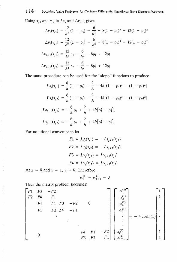
·.4 Boundary-Value Problems for Ordinary Differential Equations: Finite Element Methods
Using TjI and Tj2 in LVj and LVj+ 1 gives
12 6= h2 (1 - PI) - h2 - 8(1 - PI? + 12(1 - Pl)2
12 6= h2 (1 - P2) - h2 - 8(1 - P2)3 + 12(1 - P2)2
_ 12 6 3 2 2- h2 PI - h2 - 8Pl + 1 PI
_ 12 6 3 12 2P 8p + P2- h2 2 - h2 - 2
The same procedure can be used for the "slope" functions to produce
6 2LSiTjl) = h (1 - PI) - h - 4h[(1 - PI? - (1 PI?]
6 2LSiTj2) = h (1 - P2) - h - 4h[(1 - P2)3 - (1 - P2)2]
() 6 2 [ 3 2]Lsj + 1 Tj1 = - h PI + h + 4h PI - PI ,
() 6 2 [ 3 2]LSj + 1 Tj2 = -h P2 + h + 4h P2 - P2 .
For notational convenience let
F1 = LSiTj1) - LSj+ 1(Tj2)
F2 = LSiTj2) - LSj+ 1(Tj1)
F3 = LV/Tj2) = LVj+ 1(TjI)
F4 = LVj(Tj1) = LVj+ 1(Tj2)
At x = 0 and x = 1, Y = O. Therefore,
a (1) = a (1) = 01 e+1
Thus the matrix problem becomes:
F1 F3 -F2 a(2) 11
F2 F4 -F1 a(l) 12F4 F1 F3 -F2 0 (2)a 2
F3 F2 F4 -F1 a(l)3
- 4 cosh (1)
F4 F1 -F2 a (2) 10
e
F3 F2 -F1 (2)1a e+ 1
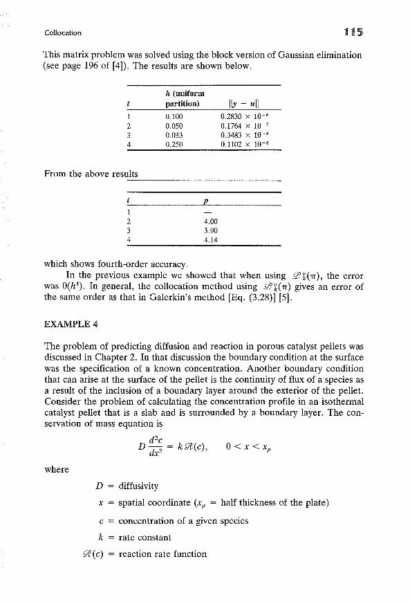
Collocation 115
This matrix problem was solved using the block version of Gaussian elimination(see page 196 of [4]). The results are shown below.
1234
From the above results
1234
h (uniformpartition)
0.1000.0500.0330.250
p
4.003.904.14
Ily - ull0.2830 X 10-6
0.1764 X 10- 7
0.3483 X 10⁻⁸
0.1102 X 10⁻⁸
0< x < xp
which shows fourth-order accuracy.In the previous example we showed that when using ..0' k(7T), the error
was O(h4). In general, the collocation method using ..0' k(7T) gives an error of
the same order as that in Galerkin's method [Eq. (3.28)] [5].
EXAMPLE 4
The problem of predicting diffusion and reaction in porous catalyst pellets wasdiscussed in Chapter 2. In that discussion the boundary condition at the surfacewas the specification of a known concentration. Another boundary conditionthat can arise at the surface of the pellet is the continuity of flux of a species asa result of the inclusion of a boundary layer around the exterior of the pellet.Consider the problem of calculating the concentration profile in an isothermalcatalyst pellet that is a slab and is surrounded by a boundary layer. The conservation of mass equation is
d 2cD - = k9l(c),
dx2
where
D = diffusivity
x = spatial coordinate (xp = half thickness of the plate)
c = concentration of a given species
k = rate constant
~(c) = reaction rate function
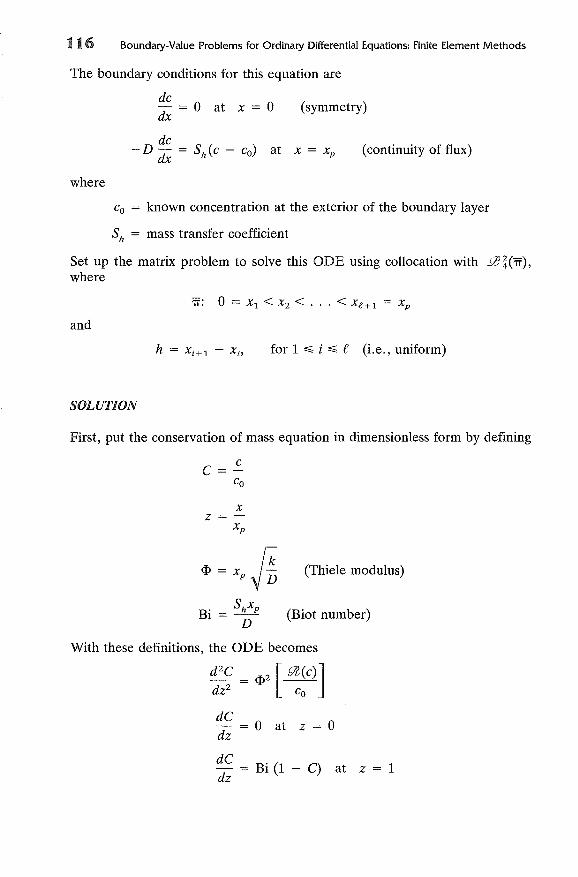
(symmetry)
116 Boundary-Value Problems for Ordinary Differential Equations: Finite Element Methods
The boundary conditions for this equation are
dc = 0 at x = 0dx
where
dc-D - = S (c - c)dx h 0
at x = Xp (continuity of flux)
Co = known concentration at the exterior of the boundary layer
Sh = mass transfer coefficient
Set up the matrix problem to solve this ODE using collocation with .cl'~(7f),
where
7f: 0 = Xl < X2 < ... < Xe+l = x p
and
for 1 ~ i ~ e (i.e., uniform)
SOLUTION
First, put the conservation of mass equation in dimensionless form by defining
C=~Co
<I> = x Jk (Thiele modulus)p D
. ShXpBl = -- (Biot number)
D
With these definitions, the ODE becomes
d2C = <1>2 [ 9l(C)]
dz2Co
dC = 0 at z = 0dz
dC = Bi (1 - C) at z = 1dz
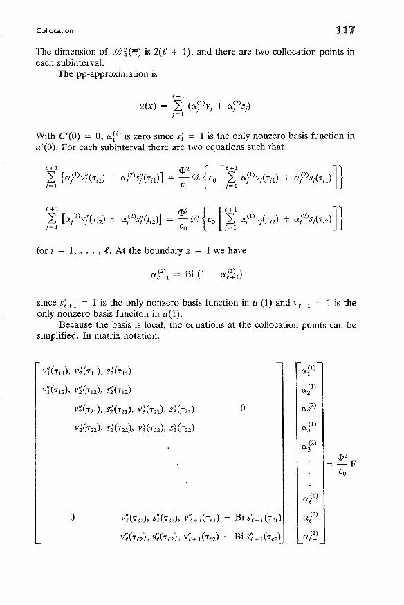
Collocation 117
The dimension of .!lJ ~ (7f) is 2(.£ + 1), and there are two collocation points ineach subinterval.
The pp-approximation is
e+1u(x) = ~ (a?)vj + a?)sj)
j=l
With C'(O) = 0, af) is zero since s~ = 1 is the only nonzero basis function inu'(O). For each subinterval there are two equations such that
for i = 1, ... , .£. At the boundary z = 1 we have
(2) B' (1 (1) )ae+ 1 = 1 - ae+ 1
since S~+l = 1 is the only nonzero basis function in u'(1) and Vf+1 = 1 is theonly nonzero basis funciton in u(1).
Because the basis is local, the equations at the collocation points can besimplified. In matrix notation:
V~(Tl1)' V~(Tl1)' S~(Tl1)a(l)
1
V~(Td, v~(Td, s~(Tda(l)
2
V~(T21)' S~(T21)' V~(T21)' S~(T21) 0 a (2)2
V~(Td, S~(T22)' V~(T22)' S~(T22)a(l)
3
a (2)3
<1>2
= -FCo
a (1)e
0 V~(Td, s~(Td, V~+l(Tf1) - Bi S~+JTf1) a (2)e
V~(Td, s~(Td, V~+l(Tf2) - Bi S~+l(Tf2)(1)
ae+1
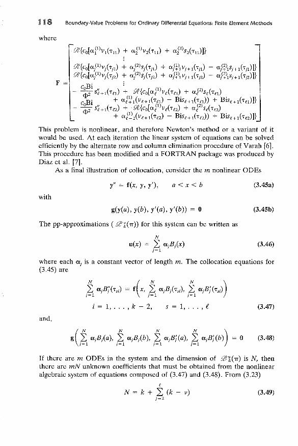
118 Boundary-Value Problems for Ordinary Differential Equations: Finite Element Methods
where
Yl'{co[aplvlrjl) + aFlSlrjl) + ag\vj+1(-rjl) + af;\Sj+l(-rjl)]}Yl'{cO[aplVj(-rj2) + aFlslrj2) + agllVj+l(Tj2) + af;llSj+l(Tj2)]}
C~i S;+l(Tn) ~ Yl'{cO[aplVe(T,:l) + aplSe(Tn)c Bi + ai~l(Ve+l(Tn) - Bise+l(Tn)) + Bise+l(Tn)]}~2 S;+l(Tn) + Yl'{cO[aplVe(Tn) + aFlse(Ta)
+ ai~1(Ve+l(Te2) - Bise+l(Tn» + Bise+l(Tn)H
This problem is nonlinear, and therefore Newton's method or a variant of itwould be used. At each iteration the linear system of equations can be solvedefficiently by the alternate row and column elimination procedure of Varah [6].This procedure has been modified and a FORTRAN package was produced byDiaz et al. [7].
As a final illustration of collocation, consider the m nonlinear ODEs
with
y" = f(x, y, y'), a<x<b (3.45a)
g(y(a), y(b), y'(a), y'(b» = 0
The pp-approximations ( il k(-lT» for this system can be written as
N
u(x) = L OljBj(x)j=l
(3.45b)
(3.46)
where each Olj is a constant vector of length m. The collocation equations for(3.45) are
and,
i = 1, ... , k - 2, S = 1, ... , .e (3.47)
(3.48)
If there are m ODEs in the system and the dimension of ilk('lT) is N, thenthere are mN unknown coefficients that must be obtained from the nonlinearalgebraic system of equations composed of (3.47) and (3.48). From (3.23)
eN = k + L (k - v)
j=2(3.49)
Collocation
and the number of coefficients is thus
mk + m(e - 1)(k - v)
119
(3.50)
The number of equations in (3.47) is m(k - 2)e, and in (3.48) is 2m. Thereforethe system (3.47) and (3.48) is composed of 2m + meek - 2) equations. If weimpose continuity of the first derivative, that is, v = 2, then (3.50) becomes
mk + m(e - 1)(k - 2)
or
2m + meek - 2) (3.51)
Thus the solution of the system (3.47) and (3.48) completely specifies the ppapproximation.
Mathematical Software
The available software that is based on collocation is rather limited. In fact, itconsists of one code, namely COLSYS [8]. Next, we will study this code in detail.
COLSYS uses spline collocation to determine the solution of the mixedorder system of equations
where
U~Ms)(X) = fs(x; z(u)),
a<x<b
s = 1, ... ,d
(3.52)
M s = order of the s differential equation
II = [Ul> Uz, ..• , UdV is the vector of solutions
z(u) = (u l , ui, ... , u~Ml-1l, ... , Ud' u~, ... , u5tMd - l))
It is assumed that the components Ul , Uz, ... , Ud are ordered such that
M l ~ M z ~ ... ~ M d ~ 4
Equations (3.52) are solved with the conditions
(3.53)
j = 1, ... ,M* (3.54)
whered
M* L M ss= 1
and
a ~ ~i ~ ~z ~ . .. ~ ~M' ~ b
Unlike the BVP codes in Chapter 2, COLSYS does not convert (3.52) to a firstorder system. While (3.54) does not allow for nonseparated boundary conditions,
t 20 Boundary-Value Problems for Ordinary Differential Equations: Finite Element Methods
such problems can be converted to the form (3.54) [9]. For example, considerthe BVP
y" = f(x, y, y'), a<x<b
y'(a) = <X, g(y(a), y(b)) = 0 (3.55)
Introducing a (constant) Vex) gives an equivalent BVP
y" = f(x, y, y'), a < x < b
V' = 0, (3.56)
y'(a) = <X, yea) = V(a), g(V(b), y(b)) = 0
which does not contain a nonseparated boundary condition.COLSYS implements the method of spline collocation at Gaussian points
using a B-spline basis (modified versions of deBoor's algorithms [2] are used tocalculate the B-splines and their derivates). The pp-solutions are thus in !lJ '( ('IT)where COLSYS sets k and v* such that
where
s = 1, ... ,d (3.57)
v* = {Vj = M s I j = 2, ... , t'}
q = number of collocation points per subintervals
The matrix problem is solved using an efficient implementation of Gaussianelimination with partial pivoting [10], and nonlinear problems are "handled"by the use of a modified Newton method. Algorithms are included for estimatingthe error, and for mesh refinement. A redistribution of mesh points is automatically performed (if deemed worthwhile) to roughly equidistribute the error.This code has proven to be quite effective for the solution of "difficult" BVPsarising in chemical engineering [11].
To illustrate the use of COLSYS we will solve the isothermal effectivenessfactor problem with large Thiele moduli. The governing BVP is the conservationof mass in a porous plate catalyst pellet where a second-order reaction rate isoccurring, i.e.,
d 2c _ rF.2 2dx2 - 'J! C , 0 < x < 1,
C'(O) = 0
c(l) = 1 (3.58)where
c = dimensionless concentration of a given species
x = 'dimensionless coordinate
<I> = Thiele modulus (constant)
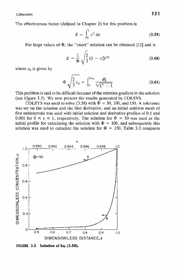
Collocation
The effectiveness factor (defined in Chapter 2) for this problem is
E = L1
c2 dx
121
(3.59)
For large values of <1>, the "exact" solution can be obtained [12] and is
where Co is given by
1 J2E = ~ 3" (1 - C6)1/2 (3.60)
<I> J~3 Co = (lleo d~ (3.61)
Jo V~3 -: 1
This problem is said to be difficult because of the extreme gradient in the solution(see Figure 3.5). We now present the results generated by COLSYS.
COLSYS was used to solve (3.58) with <I> = 50, 100, and 150. A tolerancewas set on the solution and the first derivative, and an initial uniform mesh offive subintervals was used with initial solution and derivative profiles of 0.1 and0.001 for 0 ~ x ~ 1, respectively. The solution for <I> = 50 was used as theinitial profile for calculating the solution with <I> = 100, and subsequently thissolution was used to calculate the solution for <I> = 150. Table 3.3 compares
xI.°,-0_,9,9_0__0_,9,9_2__0.:,:,,9.:,:94-'-------'0'--,9,9_6_----'0_,9,9_8_--:::;"",1.0
u~
Z0I- 0.8«0::I-ZWU 0,6Z0U
(j)(j)
0.4w.-JZ0u;Z 0.2w::2:0
DIMENSIONLESS DISTANCE,x
fiGURE 3.5 Solution of E.q. (3.58).
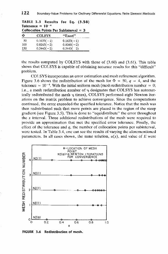
122 Boundary-Value Problems for Ordinary Differential E.quations: Finite E.lement Methods
TABLE. 3.3 Results for Eq. (3.58)Tolerance = 10-4
Collocation Points Per Subinterval = 3
50100150
COLSYS
0.1633( -1)0.8165( -2)0.5443( -2)
"Exact"0.1633( -1)0.8165( -2)0.5443( -2)
the results computed by COLSYS with those of (3.60) and (3.61). This tableshows that COLSYS is capable of obtaining accurate results for this "difficult"problem.
COLSYS incorporates an error estimation and mesh refinement algorithm.Figure 3.6 shows the redistribution of the mesh for <I> = 50, q = 4, and thetolerance = 10-4
• With the initial uniform mesh (mesh redistribution number = 0;i.e., a mesh redistribution number of 1) designates that COLSYS has automatically redistributed the mesh 1) times), COLSYS performed eight Newton iterations on the matrix problem to achieve convergence. Since the computationscontinued, the error exceeded the specified tolerance. Notice that the mesh wasthen redistributed such that more points are placed in the region of the steepgradient (see Figure 3.5). This is done to "equidistribute" the error throughoutthe x interval. Three additional redistributions of the mesh were required toprovide an approximation that met the specified error tolerance. Finally, theeffect of the tolerance and q, the number of collocation points per subinterval,were tested. In Table 3.4, one can see the results of varying the aforementionedparameters. In all cases shown, the same solution, u(x), and value of E were
CD =LOCATION OF MESHPOINT
NI(a)=a NEWTON ITERATIONS
NI(ll FOR CONVERGENCE
NI(])
NI(])
NI(l)
NI(8)
~wCD 4~~
zzoi= 3~
CD~
~ 2oW~
:c(/)w~
oo 0.2 0.4
x0.6 0.8 1.0
FIGURE 3.6 Redistribution of mesh.
Collocation
TABU 3.4 further Results for £q. (3.58)«P = 50
123
Collocation PointsPer Subinterval3324
Number ofSubintervals
201148012
Tolerance onSolution andDerivative10-4
10- 6
10- 4
10-4
E.T.R.*
1.04.61.91.1
* E.T.R. = execution time ratio.
obtained. As the tolerance is lowered, the number of subintervals and the execution time required for solution increase. This is not unexpected since we areasking the code to calculate a more accurate solution. When q is raised from 3to 4, there is a slight decrease in the number of subintervals required for solution,but this requires approximately the same execution time. If q is reduced from3 to 2, notice the quadrupling in the number of subintervals usedfor solution and also the approximate doubling of the execution time. The drastic changes in going from q = 2 to q = 3 and the relatively small changes whenincreasing q from 3 to 4 indicate that for this problem one should specify q ~ 3.
In this chapter we have outlined two finite element methods and havediscussed the limited software that implements these methods. The extensionof these methods from BVPs to partial differential equations is shown in laterchapters.
PROBLEMS
1. A liquid is flowing in laminar motion down a vertical wall. For z < 0, thewall does not dissolve in the fluid, but for 0 < z < L, the wall contains aspecies A that is slightly soluble in the liquid (see Figure 3.7, from [13]).In this situation, the change in the mass convection in the z directionequals the change in the diffusion of mass in the x direction, or
~ (UZcA ) = D a2
c A
az ax 2
where U z is the velocity and D is the diffusivity. For a short "contact time"the partial differential equation becomes (see page 561 of [13]):
ax aCA = D a2cA
az ax2
CA = 0 at z = 0
CA = 0 at x = 00
CA c1 at x = 0
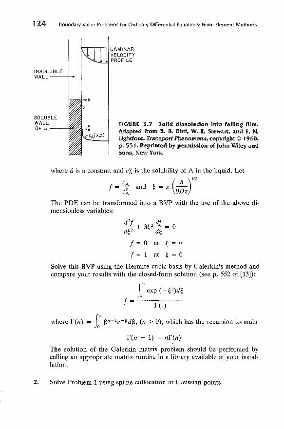
• 24 Boundary-Value Problems for Ordinary Differential Equations: Finite Element Methods
h-.,---,--"; LAMIN ARVELOCITYPROFILE
INSOLUBLEWALL--+-O-
SOLUBLEWALLOF A
x
fiGURE 3.7 Solid dissolution Into failing film.Adapted from R. B. Bird, W. E. Stewart, and E. N.Lightfoot, Transport Phenomena, copyright © 1960,p. 551. Reprinted by permission of John Wiley andSons, New York.
where f(n)
where a is a constant and c1 is the solubility of A in the liquid. Let
f = CAand ~ = x (~)1/3c1 9Dz
The PDE can be transformed into a BVP with the use of the above dimensionless variables:
d2f + 3e df = 0
de d~
f = 0 at ~ = 00
f = 1 at ~ = 0
Solve this BVP using the Hermite cubic basis by Galerkin's method andcompare your results with the closed-form solution (see p. 552 of [13]):
fi;x exp ( - ~3)d~
f= fmLX I3n-1r13dl3, (n > 0), which has the recursion formula
f(n + 1) = nf(n)
The solution of the Galerkin matrix problem should be performed bycalling an appropriate matrix routine in a library available at your installation.
2. Solve Problem 1 using spline collocation at Gaussian points.
Problems 125
3.* Solve problem 5 of Chapter 2 and compare your results with those obtainedwith a discrete variable method.
4.* The following problem arises in the study of compressible boundary layerflow at a point of attachment on a general curved surface [14].
f'" + (f + cg)f" + (1 + Swh - (f'F) = 0
gill + (f + cg)g" + c(l + Swh - (f')2) = 0
hlf + (f + cg)h' = 0
with
f=g=f' = g' = 0 at Tj = 0
h= 1 at Tj = 0
f' = g' = 1 at Tj ~ 00
h = 0 at Tj~oo
where f, g, and h are functions of the independent variable Tj, and c andSw are constants. As initial approximations use
Tj2f(Tj) = g(Tj) = ---2
Tjoo
h(Tj) = Tjoo - Tj
Tjoo
where Tjoo is the point at which the right-hand boundary conditions areimposed. Solve this problem with Sw = 0 and c = 1.0 and compare yourresults with those given in [11].
5.* Solve Problem 4 with Sw = 0 and c = -0.5. In this case there are twosolutions. Be sure to calculate both solutions.
6.* Solve Problem 3 with [3 = 0 but allow for a boundary layer around theexterior of the pellet. The boundary condition at x = 1 now becomes
dy = Bi (1 - y)dx
Vary the value of Bi and explain the effects of the boundary layer.
REFERENCES
1. Fairweather, G., Finite Element Galerkin Methods for Differential Equations, Marcel Dekker, New York (1978).
2. deBoor, C., Practical Guide to Splines, Springer-Verlag, New York (1978).
.26 Boundary-Value Problems for Ordinary Differential Equations: Finite Element Methods
3. Varga, R. S., Matrix Iterative Analysis, Prentice-Hall, Englewood Cliffs,N.J. (1962).
4. Fox, P. A., A. D. Hall, and N. L. Schryer, "The PORT MathematicalSubroutine Library," ACM TOMS, 4, 104 (1978).
5. deBoor, C., and B. Swartz, "Collocation at Gaussian Points," SIAM J.Numer. Anal., 10, 582 (1973).
6. Varah, J. M., "Alternate Rowand Column Elimination for Solving CertainLinear Systems," SIAM J. Numer. Anal., 13, 71 (1976).
7. Diaz, J. c., G. Fairweather, and P. Keast, "FORTRAN Packages forSolving Almost Block Diagonal Linear Systems by Alternate RowandColumn Elimination," Tech. Rep. No. 148/81, Department of ComputerScience, Dniv. Toronto (1981).
8. Ascher, D., J. Christiansen, and R. D. Russell, "Collocation Software forBoundary Value ODEs," ACM TOMS, 7, 209 (1981).
9. Ascher, D., and R. D. Russell, "Reformulation of Boundary Value Problems Into "Standard" Form," SIAM Rev. 23, 238 (1981).
10. deBoor, C., and R. Weiss, "SOLVEBLOK: A Packagefor Solving AlmostBlock Diagonal Linear Systems," ACM TOMS, 6, 80 (1980).
11. Davis, M., and G. Fairweather, "On the Dse of Spline Collocation forBoundary Value Problems Arising in Chemical Engineering," Comput.Methods. Appl. Mech. Eng., 28, 179 (1981).
12. Aris, R., The Mathematical Theory ofDiffusion and Reaction in PermeableCatalysts, Clarendon Press, Oxford (1975).
13. Bird, R. B., W. E. Stewart, and E. N. Lightfoot, Transport Phenomena,Wiley, New York (1960).
14. Poots, J., "Compressible Laminar Boundary-Layer Flow at a Point ofAttachment," J. Fluid Mech., 22, 197 (1965).
BIBLIOGRAPHY
For additional or more detailed information, see the following:
Becker, E. B., G. F. Carey, and J. T. Oden, Finite Elements: An Introduction, PrenticeHall, Englewood Cliffs, N.J. (1981).
deBoor, C., Practical Guide to Splines, Springer-Verlag, New York (1978).
Fairweather, G., Finite Element Galerkin Methods for Differential Equations, MarcelDekker, New York (1978).
Russell, R. D., Numerical Solution of Boundary Value Problems, Lecture Notes, Universidad Central de Venezuela, Publication 79-06, Caracas (1979).
Strang, G., and G. J. Fix, An Analysis of the Finite Element Method, Prentice-Hall,Englewood Cliffs, N.J. (1973).
(4.2)
Equations in One Space Variable
INTRODUCTION
In Chapt~r 1 we discussed methods for solving IVPs, whereas in Chapters 2 and3 boundary-value problems were treated. This chapter combines the techniquesfrom these chapters to solve parabolic partial differential equations in one spacevariable.
CLASSifiCATION Of PARTIAL DiffERENTIAL EQUATIONS
Consider the most general linear partial differential equation of the second orderin two independent variables:
Lw = awxx + 2bwxy + CWyy + dwx + ewy + fw = g (4.1)
where a, b, C, d, e, f, g are given functions of the independent variables andthe subscripts denote partial derivatives. The principal part of the operator Lis
a2 a2 a2
a-+2b--+c-ax2 ax ay ay2
Primarily, it is the principal part, (4.2), that determines the properties of thesolution of the equation Lw = g. The partial differential equation Lw - g = 0
127
128 Parabolic Partial Differential Equations in One Space Variable
is classified as:
HyperbOliC} {> °Parabolic according as b2
- ac = °Elliptic < ° (4.3)
where b2 - ac is called the discriminant of L. The procedure for solving eachtype of partial differential equation is different. Examples of each type are:
Wxx + W yy = 0, e.g., Laplace's equation, which is elliptic
e.g., wave equation, which is hyperbolic
e.g., diffusion equation, which is parabolic
An equation can be of mixed type depending upon the values of the parameters,e.g.,
YWxx + Wyy = 0,(Tricomi's equation) {
y < 0, hyperbolicy = 0, parabolic,U > 0, elliptic
To each of the equations (4.1) we must adjoin appropriate subsidiaryrelations, called boundary and/or initial conditions, which serve to complete theformulation of a "meaningful problem." These conditions are related to thedomain in which (4.1) is to be solved.
METHOD OF LINES
Consider the diffusion equation:
aw = D a2wat ax2 '
°< x < 1, 0< t
D constant, (4.4)
with the following mesh in the x-direction
i = 1, ... ,N
(4.5)
(4.6)
Discretize the spatial derivative in (4.4) using finite differences to obtain thefollowing system of ordinary differential equations:
duo Dd/ = h2 [Ui+l - 2ui + ui-d
where
ult) = W(Xi' t)
Method of Lines 129
Thus, the parabolic PDE can be approximated by a coupled system of ODEsin t. This technique is called the method of lines (MOL) [1] for obvious reasons.To complete the formulation we require knowledge of the subsidiary conditions.The parabolic PDE (4.4) requires boundary conditions atx = °and x = 1, andan initial condition at t = 0. Three types of boundary conditions are:
Dirichlet, e.g., weD, t) = 8l(t)
Neumann, e.g., wi1, t) = gz(t)
Robin, e.g., aw(O, t) + I3wx (O, t) = git) (4.7)
In the MOL, the boundary conditions are incorporated into the discretizationin the x-direction while the initial condition is used to start the associated IVP.
EXAMPLE 1
Write down the MOL discretization for
aw = D azwat axz
weD, t) = a
w(l, t) = 13
w(x, 0) = a + (13 - a)x
using a uniform mesh, where D, a, and 13 are constants.
SOLUTION
Referring to (4.6), we have
du Ddt' = hZ [u;+1 - 2u; + u;-d, i = 2, ... ,N
i = 3, ... ,N - 1
For i = 1, U 1 = a, and for i = N + 1, UN+l = 13 from the boundary conditions.The ODE system is therefore:
duz 1dt = hZ [u3 - 2uz + a]
duo 1dr' = hZ [U;+l - 2u; + u;-d,
with
u; = a + (13 - a)x; at t = °This IVP can be solved using the techniques discussed in Chapter 1.
130 Parabolic Partial Differential Equations in One Space Variable
The method of lines is a very useful technique since IVP solvers are in amore advanced stage of development than other types of differential equationsolvers. We have outlined the MOL using a finite difference discretization. Otherdiscretization alternatives are finite element methods such as collocation andGalerkin methods. In the following sections we will first examine the MOL usingfinite difference methods, and then discuss finite element methods.
FINITE DIffERENCES
Low-Order Time Approximations
Consider the diffusion equation (4.4) with
w(O, t) = 0
w(l, t) = 0
w(x, 0) = f(x)
which can represent the unsteady-state diffusion of momentum, heat, or massthrough a homogeneous medium. Discretize (4.4) using a uniform mesh to give:
duo Dd/ = h2 [Ui+l - 2ui + ui-d, i = 2, ... , N
(4.8)
where Ui = f(xi), i = 2, ... ,N at t = O. If the Euler method is used to integrate(4.8), then with
we obtain
j = 0,1, ...
or
where
Ui,j+l - Ui,j DI::i.t = h2 [Ui+1,j - 2 i ,j + Ui-1,j]
Ui,j+l = (1 - 2T)Ui ,j + T(Ui+1,j + Ui-l,)
(4.9)
AtT = h2 D
and the error in this formula is O(At + h2) (At from the time discretization, h2
from the spatial discretization). At j = 0 all the u/s are known from the initialcondition. Therefore, implementation of (4.9) is straightforward:
Finite Differences 131
1. Calculate Ui,j+1 for i = 2, ... , N (u l and UN+l are known from theboundary conditions), using (4.9) with j = O.
2. Repeat step (1) using the computed Ui,j+l values to calculate Ui ,j+2, and soon.
Equation (4.9) is called the forward difference method.
EXAMPLE 2
Calculate the solution of (4.8) with
D = 1
{
2X'f(x) =
2(1 - x),
for 0,;:.;; x ,;:.;; ~
for ~ ,;:.;; x ,;:.;; 1
Use h = 0.1 and let (1) At = 0.001, and (2) f:.t = 0.01.
SOLUTION
Equation (4.9) with h = 0.1 and At = 0.001 becomes:
Ui,j+l = 0.8ui,j + O.l(Ui+l,j + Ui-1,j) (1' = 0.1)
The solution of this equation at x = 0.1 and t = 0.001 is
U2,1 = 0.8~,o + 0.1(u3,o + Ul,O)
The initial condition gives
U2,O = 2h
U3,O = 2(2h)
U1,O = 0
Thus, U2 ,1 = 0.16 + 0.04 = 0.2. Likewise U3 ,1 = 0.4. Using U3 ,1' U2 ,1' UI,l' onecan then calculate U 2 ,2 as
~,2 = 0.2.
A sampling of some results are listed below:
0.0050.010.Q20.10
Finite-DifferenceSolution (x = 0.3)
0.59710,58220.53730.2472
AnalyticalSolution (x = 0.3)
0.59660.57990.53340.2444
132
Now solve (4.9) using h
Parabolic Partial Differential Equations in One Space Variable
0.1 and I1t = 0.01 (r = 1). The results are:
x
t 0.0 0.1 0.2 0.3 0.4 0.50.00 0 0.2 0.4 0.6 0.8 1.00.01 0 0.2 0.4 0.6 0.8 0.60.02 0 0.2 0.4 0.6 0.4 1.00.03 0 0.2 0.4 0.2 1.2 -0.20.04 0 0.2 0.0 1.4 -1.2 2.6
As one can see, the computed results are very much affected by the choice ofT.
In Chapter 1 we saw that the Euler method had a restrictive stabilitycriterion. The analogous behavior is shown in the forward difference method.The stability criterion for the forward difference method is [2]:
(4.10)
As with IVPs there are two properties of PDEs that motivate the derivation ofvarious algorithms, namely stability and accuracy. Next we discuss a methodthat has improved stability properties.
Consider again the discretization of (4.4), i.e., (4.8). If the implicit Eulermethod is used to integrate (4.8), then (4.8) is approximated by
or
Ui,j+l - Ui,j DI1t = h2 [Ui+l,j+l - 2ui ,j+l + Ui-1,j+d
Ui,j = -TUi+l,j+l + (1 + 2T)Ui ,j+l - TUi-1,j+l
(4.11)
The error in (4.11) is again O(l1t + h2). Notice that in contrast to (4.9), (4.11)is implicit. Therefore, denote
-T
and write (4.11) in matrix notation as:
1 + 2T -T-T 1 + 2T
-T
1 + 2T
U1,j+l
o
oUN+1,j+l
(4.12)
(4.13)
with U1,j+l UN+1,i+l = O. Equation (4.11) is called the backward differencemethod, and it is unconditionally stable. One has gained stability over the forward difference method at the expense of having to solve a tridiagonal linearsystem, but the same accuracy is maintained.
Finite Differences t33
To achieve higher accuracy in time, discretize the time derivative using thetrapezoidal rule:
where
aWat
j+1/Z
(4.14)
Notice that (4.14) requires the differential equation to be approximated at thehalf time level. Therefore the spatial discretization must be at the half time level.If the average of Wi,j and Wi,j+l is used to approximate Wi,j+l/Z' then (4.4)becomes
Wi,j+l - w· . DI1t ',J = 2hz [(Wi+1,j+l + Wi+1,j) -2(wi,j+l + Wi,j)
(4.15)
A numerical procedure for the solution of (4.4) can be obtained from (4.15) bytruncating O(LltZ + hZ) and is:
1 + 'T -'T12- 'T12 1 + 'T -'T12
1-'T'T12
'T121-'T 'T12
u·]
-'T12-'T12 1+'T
'T12'T12 1 - 'T
o
~(UN+l,j + UN+1,j+l) (4.16)
where U1,j' U1,j+v UN+l,j and UN+l,j+l = O. This procedure is called the CrankNicolson method, and it is unconditionally stable [2].
The Theta Method
The forward, backward, and Crank-Nicolson methods are special cases of thetheta method. In the theta method the spatial derivatives are approximated by
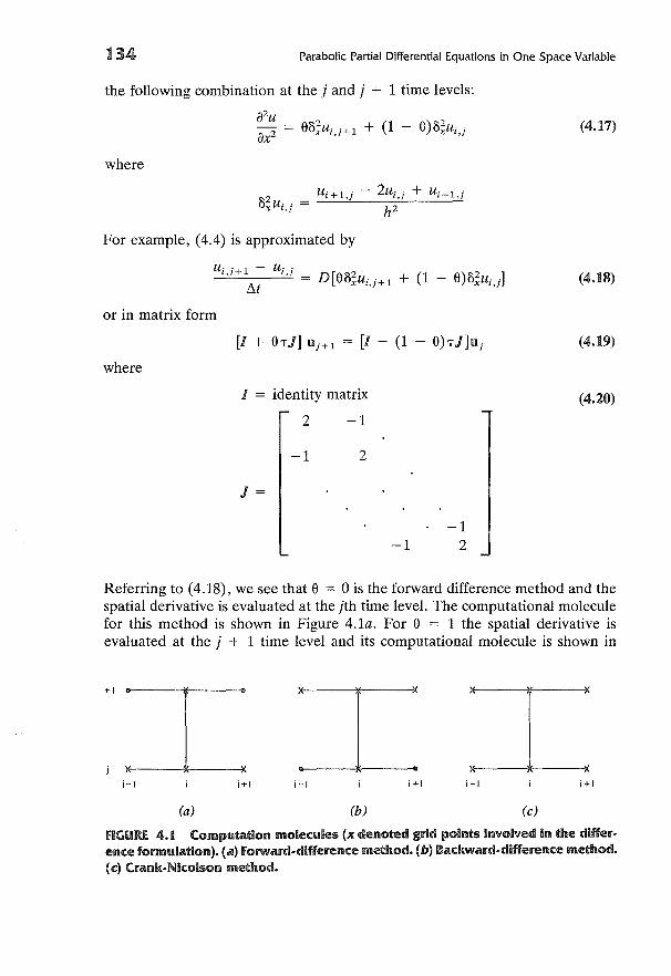
134 Parabolic Partial Differential Equations in One Space Variable
the following combination at the j and j + 1 time levels:
iPu _ 2 (1 )"2-2 - 80x u i J"+l + - 8 uxui J"ax' ,
where
U"+l " - 2u" " + U,"-l,J"02 _',J ',JxUi,j - h2
For example, (4.4) is approximated by
U i ,j+1 - Ui,j = D[802 u" " (1 8)02 ]I5..t x ',J+1 + - xUi,j
or in matrix form
(4.17)
(4.18)
[1 - (1 - 8)1"1]U j (4.19)
where
1 = identity matrix
2 -1
-1 2
J=
-1-1 2
(4.20)
Referring to (4.18), we see that 8 = 0 is the forward difference method and thespatial derivative is evaluated at the jth time level. The computational moleculefor this method is shown in Figure 4.1a. For 8 = 1 the spatial derivative isevaluated at the j + 1 time level and its computational molecule is shown in
+1
i-I
(a)
;+1 i-I
(b)
;+1 i-I
(c)
i+1
FIGURE 4.. Computation molecules (x denoted grid points involved in the difference formulation). (a) Forward-difference method. (b) Backward-difference method.(c) Crank-Nicolson method.
Finite Differences 135
Figure 4.1b. The Crank-Nicolson method approximates the differential equationat the j + ~ time level (computational molecule shown in Figure 4.1c) andrequires information from six positions. Since 8 = t the Crank-Nicolson methodaverages the spatial derivative between j and j + 1 time levels. Theta may lieanywhere between zero and one, but for values other than 0, 1, and ~ there isno direct correspondence with previously discussed methods. Equation (4.19)can be written conveniently as:
or
uj + 1 = [1 + 81"1]-1 [1 - (1 - 8) 1"1] u j (4.21)
(4.22)
Boundary and Initial Conditions
Thus far, we have only discussed Dirichlet boundary conditions. Boundary conditions expressed in terms of derivatives (Neumann or Robin conditions) occurvery frequently in practice. If a particular problem contains flux boundary conditions, then they can be treated using either of the two methods outlined inChapter 2, i.e., the method of false boundaries or the integral method. As anexample, consider the problem of heat conduction in an insulated rod with heatbeing convected "in" at x = °and convected "out" at x = 1. The problem canbe written as
aT aZTpC- = k-Pat axz
T = To at t = 0, for 0< x < 1
where
aT- k- = h1(T1 - T) at x = °
ax
aT-k- = hz(T - Tz) at x = 1
ax
T = dimensionless temperature
To = dimensionless initial temperature
pCp = density times the heat capacity of the rod
h1, hz = convective heat transfer coefficients
T1, Tz = dimensionless reference temperatures
k = thermal conductivity of the rod
(4.23)
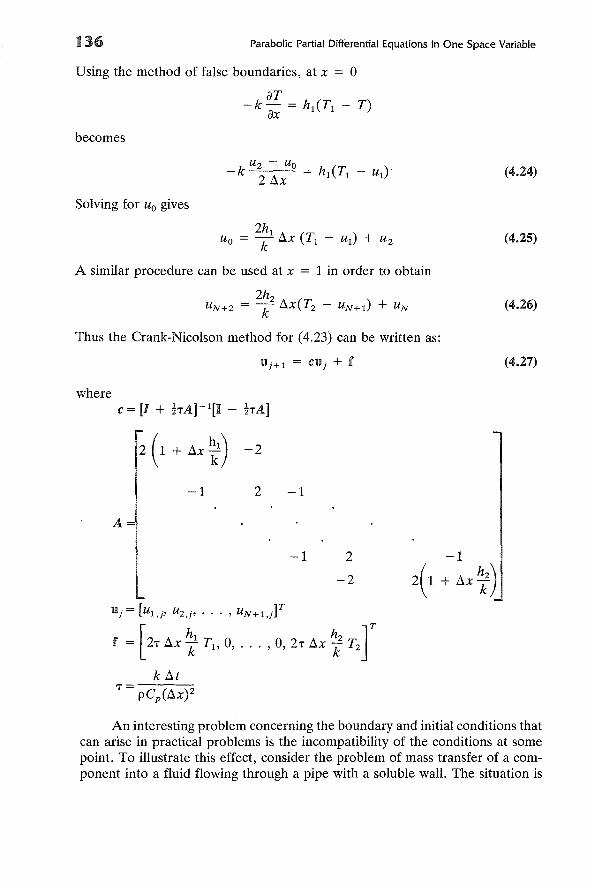
136 Parabolic Partial Differential Equations in One Space Variable
Using the method of false boundaries, at x = 0
aT-k- = h1(T1 - T)ax
becomes
Solving for Uo gives
A similar procedure can be used at x = 1 in order to obtain
2h2UN + 2 = k t:u(T2 - UN + 1) + UN
Thus the Crank-Nicolson method for (4.23) can be written as:
wherec = [I + hA]-l[I - hAl
(4.24)
(4.25)
(4.26)
(4.27)
A=
-1 2 -1
-1 2
-2
An interesting problem concerning the boundary and initial conditions thatcan arise in practical problems is the incompatibility of the conditions at somepoint. To illustrate this effect, consider the problem of mass transfer of a component into a fluid flowing through a pipe with a soluble wall. The situation is
Finite Differences 137
I' L ,
- FLUID VELOCITY
t t t t t t t t t t t t t
Fluid entersat a uniformcompositionwith molefraction ofcomponent A,
YA1 ______-L......I-.L-.L-L.....J--L---I.--L-L-L-...I-...I.-.L--'-- _
Soluble coating an wall maintains liquidcomposition Y~ next to the wall surface.
fiGURE. 4.2 Mass transfer in a pipe with a solubie wall. Adapted from R. B. Bird,W. E. Stewart, and Eo N. Lightfoot, Transport Phenomena, copyright © 1960, p. 643.Reprinted by permission of John Wiley and Sons, New York.
shown in Figure 4.2. The governing differential equation is simply a materialbalance on the fluid
vayA= 0 ~ (r ayA)az r ar ar
(a) (b)
(4.28a)
with
YA = YA , at z = 0, for °~ r ~ wall (4. 28b)
aYA = ° at r = °ar (4.28c)
at r = wall (4.28d)
where
o = diffusion coefficient
v = fluid velocity
kg = mass transfer coefficient
Term (a) is the convection in the z-direction and term (b) is the diffusion in ther-direction. Notice that condition (4.28b) does not satisfy condition (4.28d) atr = wall. This is what is known as inconsistency in the initial and boundaryconditions.
The question of the assignment of YA at z = 0, r = wall now arises, andthe analyst must make an arbitrary choice. Whatever choice is made, it introduceserrors that, if the difference scheme is stable, will decay at successive z levels(a property of stable parabolic equation solvers). The recommendation of Wilkes[3] is to use the boundary condition value and set YA = Y~ at z = 0, r = wall.
138
EXAMPLE 3
Parabolic Partial Differential Equations in One Space Variable
A fluid (constant density p and viscosity fL) is contained in a long horizontalpipe of length L and radius R. Initially, the fluid is at rest. At t = 0, a pressuregradient (Po - PL)/L is imposed on the system. Determine the unsteady-statevelocity profile V as a function of time.
SOLUTION
The governing differential equation is
p aV = Po - PL + fL!..i (r av)at L r ar ar
with
v=o at t = 0, for 0 :%; r :%; R
av = 0 at r = 0, for t ~ 0arV=o at r = R, for t ~ 0
Define
r~ =
R
T) = (Po - PL)R2
then the governing PDE can be written as
aT) = 4 + !..i (~ aT))aT ~ a~ a~
T) = 0 at T = 0, for 0 :%; ~ :%; 1
a1] = 0 at ~ = 0, for T ~ 0a~
1] = 0 at ~ = 1, for T ~ 0
At T ---? 00 the system attains steady state, 1]0C" Let
The steady-state solution is obtained by solving
1 d ( d1]oc)o = 4 + ~ d~ ~ d~
Finite Differences
with
1]00 = 0 at £ = 1
a1]oo = 0 at £ = 0a£
and is 1]00 = 1 - £2. Therefore
a<l> = ! ~ (£ a<l»a'T £a£ a£
with
a<l> = 0 at £ = 0, for'T ;:?; 0a£
<1>=0 at £ = 1, for 'T ;:?; 0
<I> = 1 - £2 at 'T = 0, for 0 ~ £ ~ 1
Discretizing the above PDE using the theta method yields:
[1 + e<PA] Uj+l = [1 - (1 - e)<pA] uj
where
139
A=
-4
2 _(1 + __1__)2(i - 1)
Table 4.1 shows the results. For <P > 0.5, the solution with e = 0 diverges. As<P goes from 0.4 to 0.04, the solutions with e = 0, 1 approach the solution withe = 1. Also notice that no change in the e = 1solution occurs when decreasing<P. Since e = 0,1 areO(A'T + A£2) and e = 1is 0(A'T2 + A£2), one would expectthe behavior shown in Table 4.1. The analytical solution is given for 'T = 0.2and 0.4, but as stated in the table, it required interpolation from Bessel functiontables, and therefore is not applicable for a five-digit precision comparison withthe numerical results. The analytical solution is given to show that all the answers
140 Parabolic Partial Differential Equations in One Space Variable
TABLE 4.1 Computed <l> Values Using the Theta Method~ = 0.4
fl> = 0.4 fl> = 0.04
'I' 6=0 6=1 6=! 6=0 6=1 6=!
0.2 0.27192 0.27374 0.27283 0.27274 0.27292 0.272830.4 0.85394( -1) 0.86541( -1) 0.85967( -1) 0.8591O( -1) 0.86025( -1) 0.85968( -1)0.8 0.84197(-2) 0.86473( -2) 0.85332(-2) 0.85218(-2) 0.85446(-2) 0.85332(-2)
Analyticalt0.27230.8567( -1)
t Solution required the use of Bessel functions, and interpolation of tabular data will produce errors in thesenumbers.
are within "engineering accuracy." Finally, the unsteady-state velocity profileis shown in Figure 4.3, and is what one would expect from the physical situation.
Nonlinear EquationsConsider the nonlinear equation
W xx = F(x, t, w, wx ' wt)
o~ x ~ 1, 0 ~ t
(4.29)
1.0 r-------~-~------__,
0.8
0.6
0.4
0.2
1.0 0.8 0.4 o 0.4 0.8 1.0
fiGURE 4.3 Transient velocity profiles.
(1) 0.1(2) 0.2(3) 00
Finite Differences 141
(4.30)
with w(O, t), w(l, t), and w(x, 0) specified. The forward difference methodwould produce the following difference scheme for (4.29):
2 _ ( ui,i+l - Ui,i)8x ui ,i - F Xi' ti, Ui,i' ilXUi,i' ilt
where
If the time derivative appears linearly, (4.30) can be solved directly. This isbecause all the nonlinearities are evaluated at the jth level, for which the nodevalues are known. The stability criterion for the forward difference method isnot the same as was derived for the linear case, and no generalized explicitcriterion is available. For "difficult" problems implicit methods should be used.The backward difference and Crank-Nicolson methods are
and
1 2( (Ui,i+1 + Ui,i28x Ui,i+l + Ui,) = F Xi' ti +1/2, 2
Ui,i+\ -t Ui,i)~ilx (u i , i + 1 + U i , i ), --'-''---''l.l----'-'"-
(4.31)
(4.32)
Equations (4.31) and (4.32) lead to systems of nonlinear equations that must besolved at each time step. This can be done by a Newton iteration.
To reduce the computation time, it would be advantageous to use methodsthat handle nonlinear equations without iteration. Consider a special case of(4.29), namely,
Wxx = !lex, t, w)wt + f2(X, t, w)wx + f3(X, t, w) (4.33)
A Crank-Nicolson discretization of (4.33) gives
with
= h i +1I2 (Ui'i+~~ Ui,i)
+ hi+1I2 ilx
(Ui,i+12+ Ui,i) + f~i+1/2 (4.34)
(u· . 1 + u· .)
f i,i+ 1/2 _ .(: l,J+ l,Jn - in Xi' ti + 1/2 , 2 ' n = 1,2,3.
Equation (4.34) still leads to a nonlinear system of equations that would requirean iterative method for solution. If one could estimate ui,i+1/2' by ui,i+1/2 say,
142 Parabolic Partial Differential Equations in One Space Variable
and use it in
1 1)2 ( U . .) = t-iJ+1/2(Ui,j+1 - Ui,j)2' x U i ,j+1 + ',j 1 At
- (u .. 1 + U· .)+ t~j+1I2 Ax l,j+ 2 ',j
where
+ h j+
1I2
(4.35)
then there would be no iteration. Douglas and Jones [4] have considered thisproblem and developed a predictor-corrector method. They used a backwarddifference method to calculate Cti,j+1I2:
1)2 - -Ii j Cti,j+1/2 - Ui,j fi j A - fi j, ";,1+," - i (~t) + i ,u;,I+'" + i'
where
(4.36)
The procedure is to predict Ui,j+1/2 from (4.36) (this requires the solutionof one tridiagonal linear system) and to correct using (4.35) (which also requiresthe solution of one tridiagonal linear system). This method eliminates the nonlinear iteration at each time level, but does require that two tridiagonal systemsbe solved at each time level. Lees [5] introduced an extrapolated Crank-Nicolsonmethod to eliminate the problem of solving two tridiagonal systems at each timelevel. A linear extrapolation to obtain Ui,j+ 112 gives
Ct· '+1/2 = U· . + ~ (u· . - U· '-1)l,] l.J 1,J l,j
or
Cti,j + 1/23Ui ,j - U i ,j-1
2(4.37)
Notice that Cti ,j+1I2 is defined directly for j > 1. Therefore, the procedure is tocalculate the first time level using either a forward difference approximation orthe predictor-corrector method of Douglas and Jones, then step in time using(4.35) with Cti,j + 1/2 defined by (4.37). This method requires the solution of onlyone tridiagonal system at each time level (except for the first step), and thuswould require less computation time.
Inhomogeneous Media
Problems containing inhomogeneities occur frequently in practical situations.Typical examples of these are an insulated pipe-i.e., interfaces at the insidefluid-inside pipewall, outside pipewall-inside insulation surface, and the outside
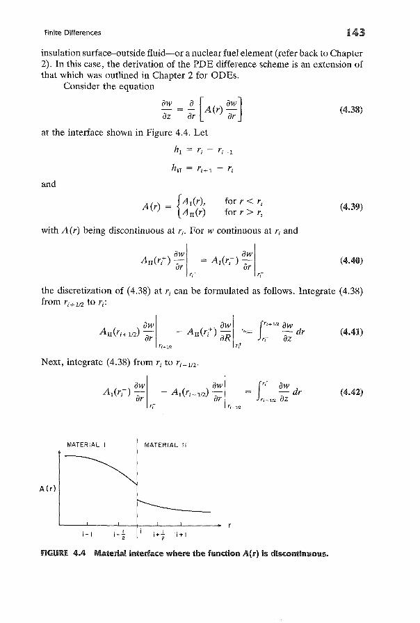
Finite Differences 143
insulation surface-outside fluid-or a nuclear fuel element (refer back to Chapter2). In this case, the derivation of the PDE difference scheme is an extension ofthat which was outlined in Chapter 2 for ODEs.
Consider the equation
ow 0 [ ow]- = - A(r)-uz or orat the interface shown in Figure 4.4. Let
and
(4.38)
A(r) = {A1(r),AlI(r)
for r < rj
for r > r i(4.39)
with A(r) being discontinuous at rj. For w continuous at r j and
+ owAlI(rj )ar (4.40)
the discretization of (4.38) at r j can be formulated as follows. Integrate (4.38)from ri+ liZ to r j :
+ aw jr'+112 aw- AlI(ri ) .oR "".= - dr
u r,+ azrt
(4.41)
Next, integrate (4.38) from r j to rj-1/Z '
rj-1I2
jr,- aw= -dr
r'-1I2 az(4.42)
A(r)
MATERIAL I MATERIAL II
i-I • 11--
2
FIGURE 4.4 Material interface where the function A(l') is discontinuous.
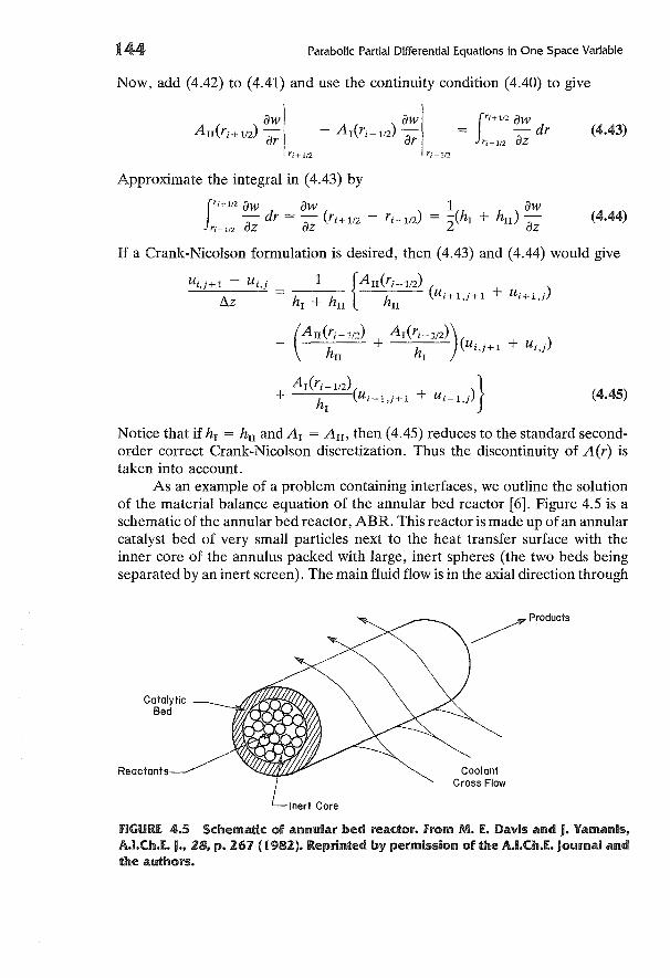
144 Parabolic Partial Differential Equations in One Space Variable
Now, add (4.42) to (4.41) and use the continuity condition (4.40) to give
fr;+112 aw
= -drr'-112 aZ
ri-l/2
(4.43)
Approximate the integral in (4.43) by
fr'+112 aw aw 1 aw
- dr = - (ri+l/Z - r i - lIZ) = -2(hr + hn ) ri-112 az az az
(4.44)
If a Crank-Nicolson formulation is desired, then (4.43) and (4.44) would give
Ui,j+l - Ui,j 1 {An (ri + 1/z)Llz = hI + hn hn (Ui+l,j+l + Ui+l)
(4.45)
Notice that if hI = hn and AI = An, then (4.45) reduces to the standard secondorder correct Crank-Nicolson discretization. Thus the discontinuity of A(r) istaken into account.
As an example of a problem containing interfaces, we outline the solutionof the material balance equation of the annular bed reactor [6]. Figure 4.5 is aschematic of the annular bed reactor, ABR. This reactor is made up of an annularcatalyst bed of very small particles next to the heat transfer surface with theinner core of the annulus packed with large, inert spheres (the two beds beingseparated by an inert screen). The main fluid flow is in the axial direction through
CatalyticBed
Reactants CoolantCross Flow
FIGURE. 4.5 Schematic of annular bed reactor. From M. E. Davis and J. Yamanis,A.I.Ch.E. J., 28, p. 267 (1982). Reprinted by permission ofthe A.I.Ch.E. Journal andthe authors.
Finite Differences 145
the core, where the inert packing promotes radial transport to the catalyst bed.If the effects of temperature, pressure, and volume change due to reaction onthe concentration and on the average velocity are neglected and mean propertiesare used, the mass balance is given by
"at _VI az
(a)
[Am An] ~ ~ (rD at)Re Sc r ar ar
(b)
+ [~: ~n}2 4> 2R(f)
(c) (4.46)
where the value of 1 or 0 for ~1 and ~2 signifies the presence or absence of aterm from the above equation as shown below
Core Screen Bed
with
1o
oo
o-1
t = dimensionless concentration
z = dimensionless axial coordinate
r = dimensionless radial coordinate
Am, An = aspect ratios (constants)
Re = Reynolds number
Sc = Schmidt number
D = dimensionless radial dispersion coefficient
4> = Thiele modulus
R(f) = dimensionless reaction rate function.
Equation (4.46) must be complemented by the appropriate boundary and initialconditions, which are given by
at r = 0at = 0ar
Dc atl = Dsc atl at r = rscar c ar sc
Dsc atl = DB atl at r = r Bar sc ar B
at = 0 at r = 1ar
(centerline)
(core-screen interface)
(screen-bed interface)
(wall)
t = 1 at z = 0, for 0 ~ r ~ 1

146 Parabolic Partial Differential Equations in One Space Variable
Notice that in (4.46), term (a) represents the axial convection and therefore isnot in the equation for the screen and bed regions, while term (c) representsreaction that only occurs in the bed, i.e., the equation changes from parabolicto elliptic when moving from the core to the screen and bed. Also, notice thatD is discontinuous at r sc and rB • This problem is readily solved by the use of anequation of the form (4.45). Equation (4.46) becomes
81
[Ui ,j+1 :z Ui ,j-1] [Am An] 1 ~ {ri + 1/z D i + 1/Z
= Re Sc hI + hrr
ri
hrr
(Ui + 1,j+1
(ri+1/Z Di+lIZ + r i - 1/Z D i - lIZ) ( . . . .)+ Ui + 1 ) - h h U"j+1 + U"j
rr I
(4.47)
with the requirement that the positions r sc and rB be included in the set of meshpoints rio Since R(Ui+ liZ) is a nonlinear function of Ui+ liZ' the extrapolated CrankNicolson method (4.37) was used to solve (4.47), and typical results from Daviset al. [7] are shown in Figure 4.6. For a discussion of the physical significanceof these results see [7].
1.0
0.9
0.8
0.7
0.6
f 0.5
0.4
0.3
0.2FLOW
( I) Laminar - Unpacked
0.1 (2) Packed Core
00 0.1
r
flGURf. 4.6 Results of annular bed reactor. Adapted from M. E. Davis, G. fairweather, and J. Yamanis, Can. J. Chem. Eng., 59, p. 499 (1981). Reprinted by permission of the Can. J. Chem. Eng.lC.S.Ch.E. and the authors.
Finite Differences 147
(4.48)
High-Order Time Approximations
Selecting an integration method for use in the MOL procedure is very importantsince it influences accuracy and stability. Until now we have only discussedmethods that are O(6.t) or O(6.tZ). Higher-order integration methods, such asRunge-Kutta, and multistep methods can be used in the MOL procedure, andin fact are the preferred methods in commercial MOL software. The formulationof the MOL-IVP leads to a system of the form:
duB - + Au = f
dt
uJO) = <Xo(xi)
where u(t) is the vector of nodal solution values at grid points of the mesh (Xi),A corresponds to the spatial operator, f can be a nonlinear function vector, and<Xo(xi) are the nodal solution values at the grid points for t = O. More generally,(4.48) can be written as:
dudt = g(t, u)
It is the eigenvalues of the Jacobian J,
J = agau
(4.49)
(4.50)
that determine the stiffness ratio, and thus the appropriate IVP technique.Sepehrnoori and Carey [8] have examined the effect of the IVP solver on
systems of the form (4.48) arising from PDEs by using a nonstiff (ODE [9]), astiff (DGEAR [10]), and a stabilized Runge-Kutta method (M3RK [11]). Theirresults confirm that nonstiff, moderately stiff, and stiff systems are most effectively solved by nonstiff, stabilized explicit, and stiff algorithms respectively.Also they observed that systems commonly encountered in practice require bothstiff and nonstiff integration algorithms, and that a system may change from stiffto nonstiff or vice versa during the period of integration. Some integrators suchas DGEAR offer both stiff and nonstiff options, and the choice is left to theuser. This idea merits continued development to include stiffness detection andthe ability to switch from one category to another as a significant change instiffness is detected. Such an extension has been developed by Skeel and Kong[12]. More generalizations of this type will be particularly useful for developingefficient MOL schemes.
Let us examine the MOL using higher-order time approximations by considering the time-dependent mass and energy balances for a porous catalystparticle. Because of the large amount of data required to specify the problem,consider the specific reaction:
C6H 6 (benzene) + 3Hz (hydrogen) = C6H 12 (cyclohexane)
148 Parabolic Partial Differential Equations in One Space Variable
(4.51)
(hydrogen)
(benzene)
which proceeds with the aid of a nickel/kieselguhr catalyst. The material andenergy balances for a spherical catalyst pellet are:
E aCB = De ~ (r2 aCB ) - RBat r2 ar ar
E aCH = De ~ (r2 aCH) - 3RBat r2 ar ar
aT ke a ( aT)pC - = -- r2 - + (-AH)R Bp at r2 ar ar
with
aCB = aCH = aT = ° atar ar ar r = °
De a~H = kg[C~(t) - CH ]
. aTke a; = hg[TO(t) - T]
at r = 1
CB = ° at t = 0,
CH = ° at t = 0, for °"'S r "'S rp
T = TO(O) at t = 0, for °"'S r "'S rp
where
- AH = heat of reaction
E = void fraction of the catalyst pellet
CB , CH = concentration of benzene, hydrogen
T = temperature
De = effective diffusivity (assumed equal for B and H)
ke = effective thermal conductivity
p = density of the fluid-solid system
Cp = heat capacity of the fluid-solid system
r = radial coordinate; rp = radius of the pellet
t = time
kg = mass transfer coefficient
hg = heat transfer coefficient
RB = reaction rate of benzene, RB = RB(CB, CH , T)
Finite Differences 149
and the superscript 0 represents the ambient conditions. Notice that C~, CfJ-I,and TO are functions of time; i.e., they can vary with the perturbations in areactor. Define the following dimensionless parameters
-~YB - C~(O)
CHYH = C~(O)
Te = TO(O)
Substitution of these parameters into the transport equations gives:
ae 1 a ( ae)Le - = - - x 2 - + ~<!>2 9taT x2 ax ax
with
aYB = aYH = ae = 0 at x = 0ax ax ax
(4.52)
(4.53)
at x = 1
YB = 0 at T = 0,
YH = 0 at T = 0,
e = 1 at T = 0,
for 0 ~ x ~ 1
for 0 ~ x ~ 1
for 0 ~ x ~ 1
150
where
Parabolic Partial Differential Equations in One Space Variable
2
<1>2 = C~~;)De RB(C~(O), C~(O), TO(O)) (Thiele modulus squared)
p = De ( - LlH)C~(O) (Prater number)keTO(O)
(Lewis number)
DetT=-
r~E
Bim
= rpkg
De
B. rphgIh =
ke
(dimensionless time)
(mass Biot number)
(heat Biot number)
(4.54)
For the benzene hydrogenation reaction, the reaction rate function is [13]:
Peatk K exp [(QR:rE
)]PBPH
RB =
1 + K exp (R~T)PBwhere
k = 3207 gmole/(sec'atm'gcat)K = 3.207 X 10⁻⁸ atm- 1
Q = 16,470 callgmole
E = 13,770 cal/gmole
Rg = 1.9872 call(gmoleoK)
Peat = 1.88 g/cm3
Pi = partial pressure of component i
Noticing that
Ci Pi (TO(O))Yi = q(O) = P?(O) -r/LJ [(1 1)] 2 __[~l_+_K_P--,~:::...;(--,-O)_e-"xp--,(~(X=l),,--]_YL· = exp (X2 - - 6 YBYH
6 [1 + KP~(O) exp (~l) YB6]
(4.55)
Finite Differences
where
a - Q1 - R
gTO(O)
a _ ..o..::(Q=----_E--'-)2 - R
gTO(O)
151
(use false boundaries)
We solve this system of equations using the MOL. First, the system iswritten as an IVP by discretizing the spatial derivatives using difference formulas.The IVP is:
aYB,l _ 6 2----a;- - h2 [YB,2 - YB,d - <I> 9(1
aYH,l _ 6 2 C~(O)----a;- - h2 [YH,2 - YH,l] - 3<1> C~(O) 9(1
ae 6Le _1 = h
2[e2 - e1] + 13<1>2 9( 1
aT
a~~'i = ~2 {[1 + (i ~ 1)}B,i+1 - 2YB,i +
a~:'i = ~2 {[1 + (i ~ 1)}H,i+1 - 2YH,i
[ 1] }_3.1,.2 C~(O) 9(.+ 1 - (i _ 1) YH,i-1 't' C~(O) I
Le ~; = ~2 {[1 + (i ~ 1)]ei + 1 - 2ei
+ [1 - (i ~ 1)Jei-1} + 13<1>29(i (4.56)
with i = 2, ... , N,
aYB,N+1 = ~ {2 - 2[1 +aT h2 YB,N
aYH,N+1 1{ [( 1).]aT = h2 2YH,N - 2 1 + 1 + N Blmh YH,N+1
. C~(t) [ 1]} 2 C~(O)+ 2Blmh CMO) 1 + IV - 3<1> C~(O) flP N + 1
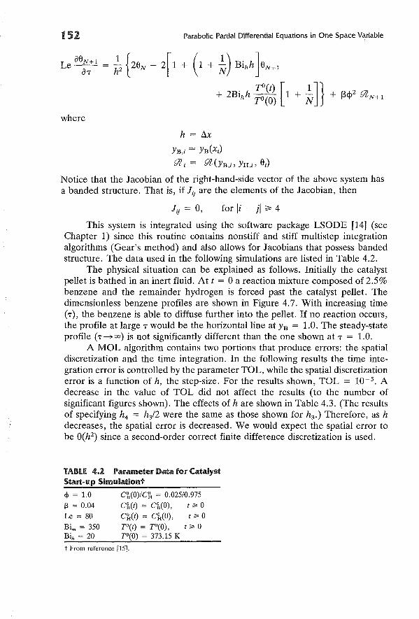
151 Parabolic Partial Differential Equations in One Space Variable
Le aeN + 1 = ~ {2e - 2[1 +aT h2 N
where
h = Ax
YB,i = YB(Xi)
[7(. = [7(. (YB' YH' e.)1 ,1' ,1' 1
Notice that the Jacobian of the right-hand-side vector of the above system hasa banded structure. That is, if Jij are the elements of the Jacobian, then
for Ii - jl ;;,: 4
This system is integrated using the software package LSODE [14] (seeChapter 1) since this routine contains nonstiff and stiff multistep integrationalgorithms (Gear's method) and also allows for Jacobians that possess bandedstructure. The data used in the following simulations are listed in Table 4.2.
The physical situation can be explained as follows. Initially the catalystpellet is bathed in an inert fluid. At t = aa reaction mixture composed of 2.5%benzene and the remainder hydrogen is forced past the catalyst pellet. Thedimensionless benzene profiles are shown in Figure 4.7. With increasing time(T), the benzene is able to diffuse further into the pellet. If no reaction occurs,the profile at large T would be the horizontal line at YB = 1.0. The steady-stateprofile (T-i>OO) is not significantly different than the one shown at T = 1.0.
A MOL algorithm contains two portions that produce errors: the spatialdiscretization and the time integration. In the following results the time integration error is controlled by the parameter TaL, while the spatial discretizationerror is a function of h, the step-size. For the results shown, TaL = 10-5 • Adecrease in the value of TaL did not affect the results (to the number ofsignificant figures shown). The effects of h are shown in Table 4.3. (The resultsof specifying h4 = h3/2 were the same as those shown for h3 .) Therefore, as hdecreases, the spatial error is decreased. We would expect the spatial error tobe O(h2
) since a second-order correct finite difference discretization is used.
TABU 4.2 Parameter Data for CatalystStart-up Simulationt
q, = 1.0 C\'.(O)/C~ = 0.025/0.975
f3 = 0.04 C\'.(t) = q(O), t ~ 0
Le = 80 C~(t) = C~(O), t ~ 0Bim = 350 TO(t) = TO(O) , t ~ 0Bih = 20 TO(O) = 373.15 K
t From reference [15].
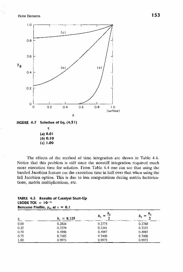
Finite Elements
1.0 ,.-------,.----,--------,.----,------::All
153
(c)
0.8
0.6
(b)
0.4
0.2
O'--------'------.l.---=-----'------'o 0.2 0.4 0.6 0.8 1.0
(surface)
x
fiGURE. 4.7 Solution of Eq. (4.51)
!(a) 0.01(b) 0.10(c) 1.00
The effects of the method of time integration are shown in Table 4.4.Notice that this problem is stiff since the nonstiff integration required muchmore execution time for solution. From Table 4.4 one can see that using thebanded Jacobian feature cut the execution time in half over that when using thefull Jacobian option. This is due to less computations during matrix factorizations, matrix multiplications, etc.
TABLE 4.3 Results of Catalyst Start-UpLSODE TOL = 10- 5
Benzene Profile, Yn, at 'T = 0.1
h _ hI hzh3 =-X hI = 0.125 z - 2 2
0.00 0.2824 0.2773 0.27600.25 0.3379 0.3341 0.33310.50 0.4998 0.4987 0.49830.75 0.7405 0.7408 0.74081.00 0.9973 0.9973 0.9973
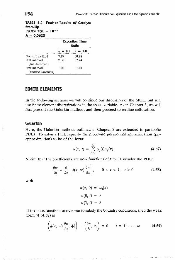
154 Parabolic Partial Differential Equations in One Space Variable
TABLE 4.4 further Results of CatalystStart-Up150D£ TOt = 10-5
h = 0.0625
Execution TimeRatio
Nonstiff methodStiff method
(full Jacobian)Stiff method
(banded Jacobian)
T = 0.1
7.872.30
1.00
T = 1.0
50.982.24
1.00
fiNITE ELEMENTS
In the following sections we will continue our discussion of the MOL, but willuse finite element discretizations in the space variable. As in Chapter 3, we willfirst present the Galerkin method, and then proceed to outline collocation.
Galerkin
Here, the Galerkin methods outlined in Chapter 3 are extended to parabolicPDEs. To solve a PDE, specify the piecewise polynomial approximation (ppapproximation) to be of the form:
m
u(x, t) 2: uj(t)<I>j(x)j=l
(4.57)
Notice that the coefficients are now functions of time. Consider the PDE:
with
aw a [ aw]at = ax a(x, w) ax ' 0< x < 1, t> 0 (4.58)
w(x, 0) = woCx)
w(O, t) = 0
w(l, t) = 0
If the basis functions are chosen to satisfy the boundry conditions, then the weakform of (4.58) is
(a(x, w) ~:' <1>;) + (aa~' <l>i) = 0 i = 1, ... m (4.59)
Finite Elements 155
The MOL formulation for (4.58) is accomplished by substituting (4.57) into(4.59) to give
i = 1, ... ,m
Thus, the IVP (4.60) can be written as:
Ba'(t) + D(a)a(t) = 0
with
Ba(O) 13where
Di,j = (a <1>; , <1>;)
Bi,j = (<I>j' <l>i)13 = [(wo, <1>1), (wo, <1>2), ..• , (wo, <l>m))T
(4.60)
(4.61)
(4.62)
In general this problem is nonlinear as a result of the function a in thematrix D. One could now use an IVP solver to calculate a(t). For example, ifthe trapezoidal rule is applied to (4.61), the result is:
[an+1 an]B l:i.t + D(an+1/2)an+1
/2 = 0
with
where
tn = n l:i.t
an = a(tn)
a n + 1/2 =2
Since the basis <l>i is local, the matrices Band D are sparse. Also, recall that theerror in the Galerkin discretization is O(hk ) where k is the order of the approximating space. Thus, for (4.62), the error is 0(l:i.t2 + hk ), since the trapezoidalrule is second-order accurate. In general, the error of a Galerkin-MOL discretization is O(l:i.tP + hk ) where p is determined by the IVP solver. In the followingexample we extend the method to a system of two coupled equations.
EXAMPLE 4
A two-dimensional model is frequently used to describe fixed-bed reactors thatare accomplishing highly exothermic reactions. For a single independent reaction
156 Parabolic Partial Differential Equations in One Space Variable
a material and energy balance is sufficient to describe the reactor. These continuity equations are:
r af = pe[~ (r af)] + 131r9P(f, e)
az ar ar
ae [a ( ae)]r - = Bo - r - + I37.r9P(f, e)az ar ar
with
f = e = 1 at z = 1, for 0 < r < 1
af = ae = 0 at r = 0, for 0 < z < 1ar ar
where
aear
-Bi(e - ew) at r = 1, for 0 < Z < 1
z = dimensionless axial coordinate, 0 ~ z ~ 1
r = dimensionless radial coordinate, 0 ~ r ~ 1
f = dimensionless concentration
e = dimensionless temperature
ew = dimensionless reactor wall temperature
9P = dimensionless reaction rate function
Bi, Pe, Bo, 131, 132 = constants
These equations express the fact that the change in the convection is equal tothe change in the radial dispersion plus the change due to reaction. The boundarycondition for e at r = 1 comes from the continuity of heat flux at the reactorwall (which is maintained at a constant value of ew). Notice that these equationsare parabolic PDE's, and that they are nonlinear and coupled through the reaction rate function. Set up the Galerkin-MOL-IVP.
SOLUTION
Let
m
u(x, z) ~ a/z)<j>/x) = f(x, z)j=l
m
vex, z) = ~ "Yj(z)<j>j(x) = e(x, z)j=l
Finite Elements 151
such that
m
u(X, 0) = 2: aj(O)<I>/X) = 1.0j=1
m
VeX, 0) = 2: 'Yj(O)<I>j(X) = 1.0j=1
The weak form of this problem is
(:~, <1» = Pe [r :~<I>{ - G~ <1>:) ] + ~1( YG, <l>i)
G:, <l>i) = Bo [r ~~<I>{ - G~, <1>:) ] + ~2( YG,<I>i)
i= 1, ... ,m
where
(a, b) = fal abr dr
The boundary conditions specify that
r = 0)(:~ = 0 at r = 1 and r = 0)
(ae- = 0 atar
r at <l>i 11 = 0ar 0
r ae <l>i 11 - Bi (e - ew )<I>i(1)ar 0
Next, substitute the pp-approximations for t and e into the weak forms of thecontinuity equations to give
j~1 a; (z)(<I>j' <1>;) = -Pe [j~1 aj(z)(<I>;, <1>;)] + ~1(.Yi, <l>i)
j~1 'Y;(z)(<I>j' <l>i) = -Bo [Bi C~1 'Yj<l>/1) - ew ) <l>i(1)
+ j~1 'Y/z)(<I>;, <1>;)] + ~2(.Yi, <l>i)' i = 1, ... ,m
where
158
Denote
Parabolic Partial Differential Equations in One Space Variable
Ci,j = (<pj, <Pi)
Di,j = (<p;, <Pi)
Bi,j = <pi(l)<pj(l)
tlJi = (9t , <p;)
The weak forms of the continuity equations can now be written as:
COl.' - Pe DOl. + 131'"
C'Y' -Bo [Bi (B'Y - ew $(l)) + D'Y] + 13z'"
with 01.(0) and 'Y(O) known. Notice that this system is a set of IVPs in thedependent variables 01. and 'Y with initial conditions 01.(0) and 'Y(O). Since thebasis <Pi is local, the matrices B, C, and D are sparse. The solution of this systemgives OI.(t) and 'Y(t) , which completes the specification of the pp-approximationsu and v.
From the foregoing discussions one can see that there are two componentsto any Galerkin-MOL solution, namely the spatial discretization procedure andthe IVP solver. We defer further discussions of these topics and that of Galerkinbased software until the end of the chapter where it is covered in the sectionon mathematical software.
CollocationAs in Chapter 3 we limit out discussion to spline collocation at Gaussian points.To begin, specify the pp-approximation to be (4.57), and consider the PDE:
with
aw ( aw aZw)-- xtw--at - f " 'ax' axz ' 0< x < 1, t> 0 (4.63)
where
w = wo(x) at t = 0'hW + f3 lw' = "Il(t) at x = 01] zW + f3zw' = "Iz(t) at x = 1
i = 1,2
According to the method of spline collocation at Gaussian points, we requirethat (4.57) satisfy the differential equation at (k - M) Gaussian points persubinterval, where k is the degree of the approximating space and M is the orderof the differential equation. Thus with the mesh
o = Xl < Xz < ... < Xe+l 1 (4.64)
Finite Elements 159
Eq. (4.63) becomes
j~l u; (t)<!>j(x;) = t(X;, t, j~l u/t)<!>j(x;), j~l Uj(t)<!>; (x;), j~l Uj(t)<!>" (x;) )
i = 1, ... , m - 2 (4.65)
where
m = (k - M}e + 2
M = 2
We now have m - 2 equations in m unknown coefficients uj • The last twoequations necessary to specify the pp-approximation are obtained by differentiating the boundary conditions:
m m
'll1 L u; (t)<!>/O) + (31 L U; (t)<!>; (0) = -y~ (t)j=l j=lm m
'll2 L U; (t)<!>j(1) + (32 L U; (t)<!>; (1) = -y;(t)j=l j=l
This system of equations can be written as
Aa' (t) = F(t, a)
a(O) = a owhere
A = left-hand side of (4.65) and (4.66)
F = right-hand side of (4.65) and (4.66)
and a o is given by:
(4.66)
(4.67)
m
L Uj(O)<!>j(xi) = Wo(X;) ,j=l
1 = 1, ... ,m
Since the basis <!>j is local, the matrix A will be sparse. Equation (4.67) can nowbe integrated in time by an IVP solver. As with Galerkin-MOL, the errorproduced from collocation-MOL is O(LltP + hk) where p is specified by the IVPsolver and k is set by the choice of the approximating space. In the followingexample we formulate the collocation method for a system of two coupledequations.
EXAMPLE 5
A polymer solution is spun into an acidic bath, where the diffusion of acid intothe polymeric fiber causes the polymer to coagulate. We wish to find the concentration of the acid (in the fiber), CA , along the spinning path. The coagulationreaction is
Polymer + acid -i> coagulated polymer + salt
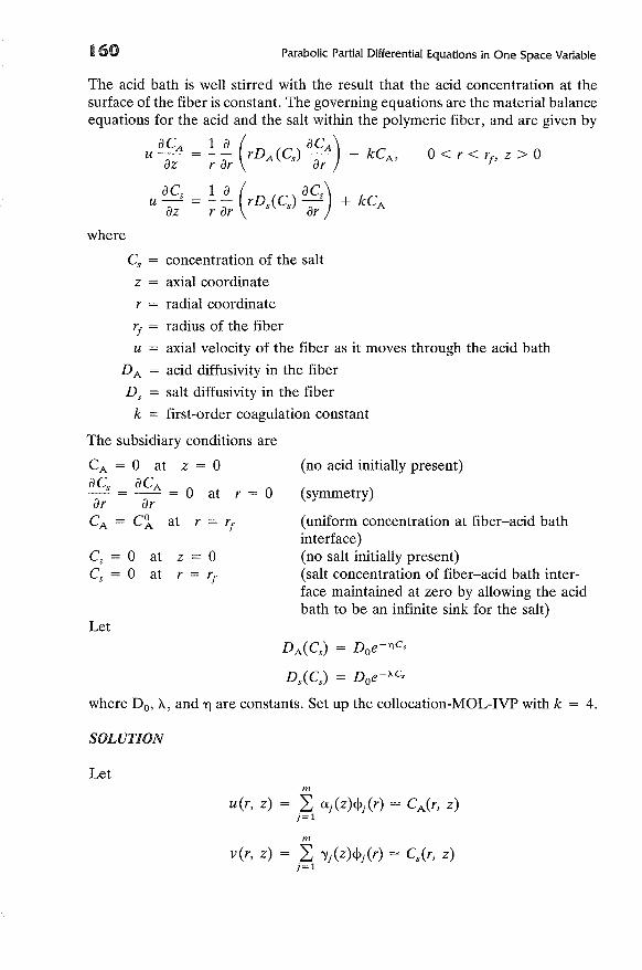
160 Parabolic Partial Differential Equations in One Space Variable
The acid bath is well stirred with the result that the acid concentration at thesurface of the fiber is constant. The governing equations are the material balanceequations for the acid and the salt within the polymeric fiber, and are given by
u aCA = ! ~ (rD (C) acA ) - kCaz r ar A s ar A, 0 < r < rf' z > 0
u acs = ! ~ (rDs(Cs) acs) + kCAaz r ar ar
where
(no acid initially present)
(symmetry)
(uniform concentration at fiber-acid bathinterface)(no salt initially present)(salt concentration of fiber-acid bath interface maintained at zero by allowing the acidbath to be an infinite sink for the salt)
Cs = 0 at z = 0Cs = 0 at r = rf
Cs = concentration of the salt
z = axial coordinate
r = radial coordinate
rf = radius of the fiber
u = axial velocity of the fiber as it moves through the acid bath
DA = acid diffusivity in the fiber
Ds = salt diffusivity in the fiber
k = first-order coagulation constant
The subsidiary conditions are
CA = 0 at z = 0acs aCA- = -- = 0 at r = 0ar arCA = Cs... at r = rf
Let
where Do, A, and'f) are constants. Set up the collocation-MOL-IVP with k = 4.
SOLUTION
Letm
u(r, z) 2: uj(z)<j>j(r) = CA(r, z)j=l
m
vCr, z) = 2: )'j(z)<j>j(r) = CsCr, z)j=l
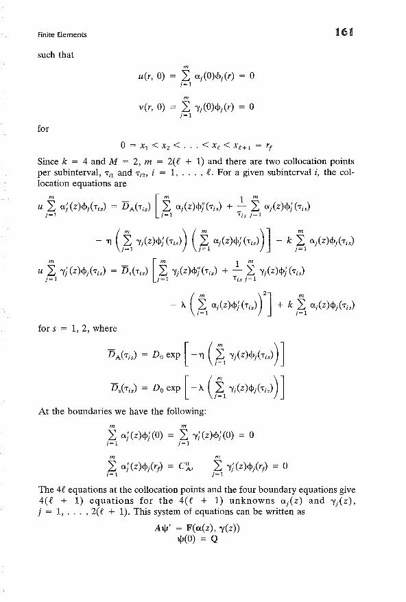
Finite Elements
such that
for
m
u(r, 0) = L Uj(O)<pj(r) = 0j=l
m
vCr, 0) = L 'Yj(O)<pj(r) = 0j=l
161
o = Xl < Xz < ... < Xe < Xe+l = rf
Since k = 4 and M = 2, m = 2(e + 1) and there are two collocation pointsper subinterval, 'Til and 'TiZ, i = 1, ... , e. For a given subinterval i, the collocation equations are
for s = 1, 2, where
DA('Tis) = Do exp [ -11 C~l 'Y/Z)<Pj('TiS)) ]
Dbis) = Do exp [ -A. (~l 'Yj (Z)<pj ('TiS)) ]
At the boundaries we have the following:
m m
L U; (Z)<p; (0) = L 1'; (Z)<p; (0) = 0j=l j=l
m
L U; (Z)<P/rf) = C~,j=l
m
L 'Y;(Z)<Pkf) = 0j=l
The 4e equations at the collocation points and the four boundary equations give4(( + 1) equations for the 4(( + 1) unknowns Uj(z) and 'Yj(Z) ,j = 1, . . . , 2(e + 1). This system of equations can be written as
AljI' = F(a(z), ')'(z))ljI(O) = Q
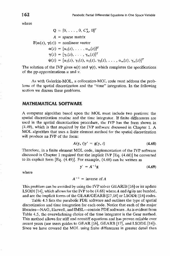
162
where
Parabolic Partial Differential Equations in One Space Variable
Q = [0, ... , 0, C~L OFA = sparse matrix
F(a(z), 'Y(z)) = nonlinear vector
a(z) = [U1(Z), , um(z))T
'Y(z) = b1(Z), , 'Vm(z))T
\fJ(z) = [U1(Z), 'V1(Z), U2(Z), 'Viz), ... , um(z), 'Vm(z)F
The solution of the IVP gives aCt) and 'Y(t), which completes the specificationsof the pp-approximations u and v.
As with Galerkin-MOL, a collocation-MOL code must address the problems of the spatial discretization and the "time" integration. In the followingsection we discuss these problems.
MATHEMATICAL SOfTWARE
A computer algorithm based upon the MOL must include two portions: thespatial discretization routine and the time integrator. If finite differences areused in the spatial discretization procedure, the IVP has the form shown in(4.49), which is that required by the IVP software discussed in Chapter 1. AMOL algorithm that uses a finite element method for the spatial discretizationwill produce an IVP of the form:
A(y, t)y' = g(y, t) (4.68)
Therefore, in a finite element MOL code, implementation of the IVP softwarediscussed in Chapter 1 required that the implicit IVP [Eq. (4.68)] be convertedto its explicit form [Eq. (4.49)]. For example, (4.68) can be written as
where
y'=A- 1g
A-I = inverse of A
(4.69)
This problem can be avoided by using the IVP solver GEARIB [16] or its updateLSODI [14], which allows for the IVP to be (4.68) where A and ag/ay are banded,and are the implicit forms of the GEAR/GEARB [17,18] or LSODE [14] codes.
Table 4.5 lists the parabolic PDE software and outlines the type of spatialdiscretization and time integration for each code. Notice that each of the majorlibraries-NAG, Harwell, and IMSL-eontain PDE software. As is evident fromTable 4.5, the overwhelming choice of the time integrator is the Gear method.This method allows for stiff and nonstiff equations and has proven reliable overrecent years (see users guides to GEAR [16], GEARB [17], and LSODE [14]).Since we have covered the MOL using finite differences in greater detail than
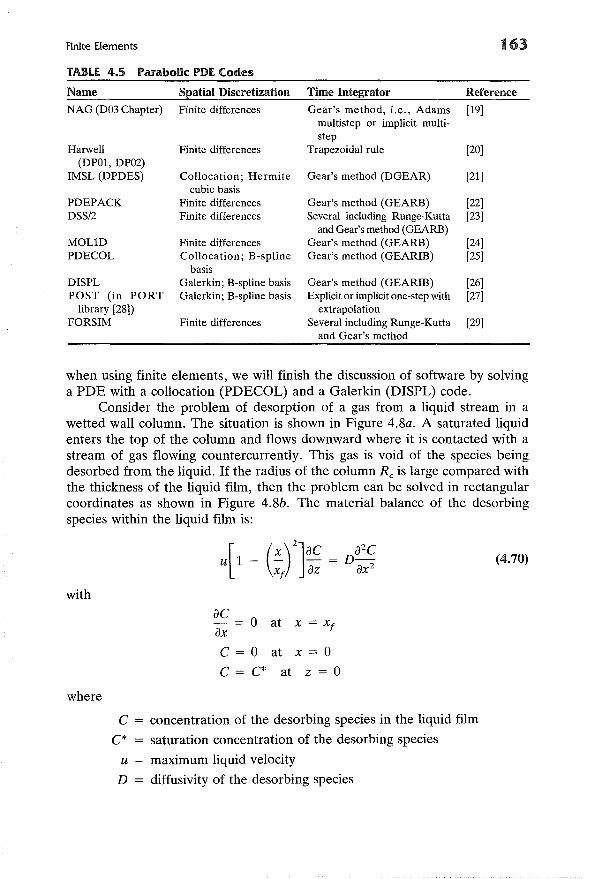
Finite Elements
TABLE 4.5 Parabolic POE Codes
163
Name
NAG (D03 Chapter)
Harwell(DP01, DP02)
IMSL (DPDES)
PDEPACKDSS/2
MOLlOPDECOL
DISPLPOST (in PORT
library [28])FORSIM
Spatial Discretization
Finite differences
Finite differences
Collocation; Hermitecubic basis
Finite differencesFinite differences
Finite differencesCollocation; B-spline
basisGalerkin; B-spline basisGalerkin; B-spline basis
Finite differences
Time Integrator
Gear's method, i.e., Adamsmultistep or implicit multistep
Trapezoidal rule
Gear's method (DGEAR)
Gear's method (GEARB)Several including Runge-Kutta
and Gear's method (GEARB)Gear's method (GEARB)Gear's method (GEARIB)
Gear's method (GEARIB)Explicit or implicit one-step with
extrapolationSeveral including Runge-Kutta
and Gear's method
Reference
[19]
[20]
[21]
[22][23]
[24][25]
[26][27]
[29]
when using finite elements, we will finish the discussion of software by solvinga PDE with a collocation (PDECOL) and a Galerkin (DISPL) code.
Consider the problem of desorption of a gas from a liquid stream in awetted wall column. The situation is shown in Figure 4.8a. A saturated liquidenters the top of the column and flows downward where it is contacted with astream of gas flowing countercurrently. This gas is void of the species beingdesorbed from the liquid. If the radius of the column Rc is large compared withthe thickness of the liquid film, then the problem can be solved in rectangularcoordinates as shown in Figure 4.8b. The material balance of the desorbingspecies within the liquid film is:
U[l (~r]~~a2c
(4.70)D-ax2
with
ac0 at x = xfax
C=O at x = 0
C = C* at z = 0
where
c = concentration of the desorbing species in the liquid film
C* saturation concentration of the desorbing species
U = maximum liquid velocity
D diffusivity of the desorbing species
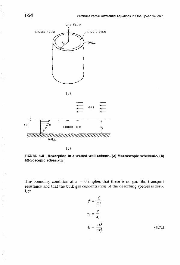
164 Parabolic Partial Differential Equations in One Space Variable
GAS FLOW
(0)
LIQUID FILM
WALL
z
~
~
~-- GAS
~-~~
.~~~Xf
WALL
(b)
fiGURE. 4.8 Desorption in a wetted-wall column. (<1) Macroscopic schematic. (11)Microscopic schematic.
The boundary condition at x = 0 implies that there is no gas film transportresistance and that the bulk gas concentration of the desorbing species is zero.Let
cf =·c*
xT] =
xf
~zD
(4.71)-ux2
f
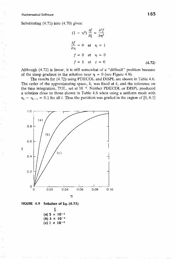
Mathematical Software
Substituting (4.71) into (4.70) gives:
(1 _ 1)2) af = a2f
a~ a1)2
af = 0 at 1) = 1a1)
f = 0 at 1) = 0
f = 1 at z = 0
165
(4.72)
Although (4.72) is linear, it is still somewhat of a "difficult" problem becauseof the steep gradient in the solution near 1) = 0 (see Figure 4.9).
The results for (4.72) using PDECOL and DISPL are shown in Table 4.6.The order of the approximating space, k, was fixed at 4, and the tolerance onthe time integration, TOL, set at 10- 6 • Neither PDECOL or DISPL produceda solution close to those shown in Table 4.6 when using a uniform mesh with1); - 1);-1 = 0.1 for all i. Thus the partition was graded in the region of [0,0.1]
1.0 .------,--~-__,_--__r-=-___,r__-__,
0.8
0.6
f
0.4
0.2
0.02 0.04 0.06 0.08 0.10
fiGURE 4.9 Solution of Eq. (4.72)
~(a) 5 x 10⁻⁵
(b) 3 x 10⁻⁴
(c) 1 X 10⁻³
166 Parabolic Partial Differential Equations in One Space Variable
TABLE 4.6 Results of (q. (4.72)1] = 0.01, k = 4, TOt = (-6)
PDECOL DISPL
5( -5) 0.6827 0.68283( -4) 0.3169 0.31681( - 3) 0.1768 0.1769'ITI: 0 = 'TJI < 'TJ2 < 'TJII = 0.1
0.1 = 'TJII < 'TJ12 < < 'TJ20 = 1.0'IT2: 0 = 'TJI < 'TJ2 < < 'TJ21 = 0.1
0.1 = 'TJ21 < 'TJ22 < 'TJ30 = 1.0
0.68390.31690.1769'TJi - 'TJi-1 = 0.01'TJi - 'TJi-1 = 0.1'TJi - 'TJi-l = 0.005'TJi - 'TJi-1 = 0.1
0.68280.31680.1769
as specified by 'lT1 and 'lTz in Table 4.6. Further mesh refinements in the regionof [0, 0.1] did not cause the solutions to differ from those shown for 'lTz. Fromthese results, one can see that PDECOL and DISPL produced the same solutions. This is an expected result since both codes used the same approximatingspace, and the same tolerance for the time integration.
The parameter of engineering significance in this problem is the Sherwoodnumber, Sh, which is defined as
where
Sh (4.73)
311
1 = 2: 0 (1 - 1]Z)f dTf (4.74)
Table 4.7 shows the Sherwood numbers for various ~ (calculated from the solutions of PDECOL using 'lTz). Also, from this table, one can see that the resultscompare well with those published elsewhere [30].
TABLE 4.7 further Results oHq. (4.72)
~ Sh* Sh (PDECOL)
5( -5) 80.75 80.731( -4) 57.39 57.383( -4) 33.56 33.555( -4) 26.22 26.228( -4) 20.95 20.941( - 3) 18.85 18.84
* From Chapter 7 of [30].
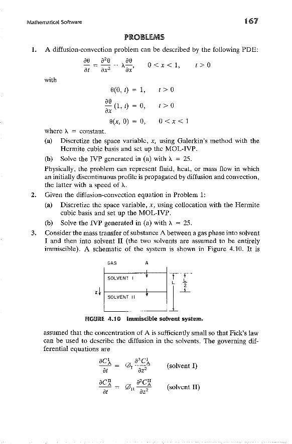
Mathematical Software
PROBLEMS
167
1. A diffusion-convection problem can be described by the following PDE:
as a2 s as'11.- 0< x < 1, t> °at ax2 ax'
with
S(O, t) = 1,
as- (1, t) = 0,ax
sex, 0) = 0,
t> °t> °O<x<l
where A = constant.(a) Discretize the space variable, x, using Galerkin's method with the
Hermite cubic basis and set up the MOL-IVP.
(b) Solve the IVP generated in (a) with A = 25.
Physically, the problem can represent fluid, heat, or mass flow in whichan initially discontinuous profile is propagated by diffusion and convection,the latter with a speed of A.
2. Given the diffusion-convection equation in Problem 1:
(a) Discretize the space variable, x, using collocation with the Hermitecubic basis and set up the MOL-IVP.
(b) Solve the IVP generated in (a) with A = 25.
3. Consider the mass transfer of substance A between a gas phase into solventI and then into solvent II (the two solvents are assumed to be entirelyimmiscible). A schematic of the system is shown in Figure 4.10. It is
GAS A
SOLVENT I' t +
zt L *----J1L
1~OLVENT II •
fiGURE 4.10 Immiscible solvent system.
assumed that the concentration of A is sufficiently small so that Fick's lawcan be used to describe the diffusion in the solvents. The governing differential equations are
ac~ a2c~(solvent I)0-at I az2
ac~ = a2c~(solvent II)0 n -
2-at az
168 Parabolic Partial Differential Equations in One Space Variable
where
e~ = concentration of A in region i (moles/cm3)
o i = diffusion coefficient in region i (cmz/s)
t = time (s)
with
e~ = e~ = 0 at t = 0
ae~-- = 0 at z = Laz
ae~0 u -z- ataz
Lz=-
2
e~ = e~ at z = L/2 (distribution coefficient = 1)
P = HeI at z = 0 (pA = partial pres.sure of A in)A A the gas phase; H IS a constant
Compute the concentration profile of A in the liquid phase from t = 0to steady state when PA = 1 atm and H = 104 atm/(moles'cm3), forDr/Du = 1.0.
4. Compute the concentration profile of A in the liquid phase (from Problem3) using DI/Du = 10.0 and DI/Du = 0.1. Compare these profiles to thecase where DI/Du = 1.0.
5*. Diffusion and adsorption in an idealized pore can be represented by thePDEs:
ac aZc- = D-z - [ka (1 - f)c - kdfJ, 0< x < 1, t> 0at ax
~ f3[ka (1 - f)c - kdfJat
with
c(O, t) = 1, t> 0
ac- (1, t) = 0, t> 0ax
c(x, 0) = f(x, 0) = 0 0<x<1
Problems
where
169
c = dimensionless concentration of adsorbate in the fluid within thepore
f = fraction of the pore covered by the adsorbate
x = dimensionless spatial coordinate
ka = rate constant for adsorption
k d = rate constant for desorption
D, f3 = constants
Let D = f3 = ka = 1 and solve the above problem with ka/kd = 0.1, 1.0,and 10.0. From these results, discuss the effect of the relative rate ofadsorption versus desorption.
6*. The time-dependent material and energy balances for a spherical catalystpellet can be written as (notation is the same as was used in the sectionFinite Differences-High-Order Time Approximations):
- <\>29(
with
where
ay = ae = ° at x = °ax axy = e = 1 at x = 1
y = 0, e = 1 at 'T = 0, for all x
(first order)
Let <\> = 1.0, f3 = 0.04, 'Y = 18, and solve this problem using:
(a) Le = 10
(b) Le = 1
(c) Le = 0.1
Discuss the physical significance of each solution.
170 Parabolic Partial Differential Equations in One Space Variable
7*. Froment [31] developed a two-dimensional model for a fixed-bed reactorwhere the highly exothermic reactions
k 1 k2
o-xylene--p.~phthalic anhydride - CO2 , CO, H20(A) "'" (B) (C)
k3 ~CO2 , CO, H20
(C)
were occurring on a vanadium catalyst. The steady-state material andenergy balances are:
aXI = Pe [a2XI + ! aXI]
az ar2 r ar
aX2 = Pe [a2X2 + ! aX2]
az ar2 r ar
ae = Bo [a2e + ! ae]
az ar2 r ar
with
0< r < 1, O<z<l
O<z<l
Xl = X2 = 0 and e = eo at z = 0,
aXI aX2 ae- = - = - = 0 at r = 0,ar ar ar
O<r<l
aXI = aX2 = 0ar ar
where
d ae B' ( )an - = 1 e - ew at r= 1,ar O<z<l
Xl = fractional conversion to B
X2 = fractional conversion to C
e = dimensionless temperature
z = dimensionless axial coordinate
r = dimensionless radial coordinate
R I = k l (l - Xl - x2) - k 2x I
R2 = k2xI + k3(1 - Xl - X2)Pe, Bo = constants
13i = constants, i = 1, 2, 3
Bi = Biot number
ew = dimensionless wall temperature
Problems 171
Froment gives the data required to specify this system of PDEs, and oneset of his data is given in Chapter 8 of [30] as:
where
Pe = 5.76,
131 = 5.106,
Bo = 10.97,
I3z = 3.144,
Bi = 2.5
133 = 11.16
with
i = 1,2,3
a1 = -1.74,
"'11 = 21.6,
a z = -4.24,
"'Iz = 25.1,
a3 = -3.89
"13 = 22.9
Let ew = eo = 1 and solve the reactor equations with:
(a) al = -1.74
(b) a1 = - 0.87
(c) a1 = - 3.48
Comment on the physical implications of your results.
8*. The simulation of transport with chemical reaction in the stratospherepresents interesting problems, since certain reactions are photochemical,i.e., they require sunlight to proceed. In the following problem let C1
denote the concentration of ozone, 03' Cz denote the concentration ofoxygen singlet, 0, and C3 denote the concentration of oxygen, Oz (assumedto be constant). If z specifies the altitude in kilometers, and a Fickianmodel of turbulent eddy diffusion (neglecting convection) is used to describe the transport of chemical species, then the continuity equations ofthe given species are
aC1 = ~[K ac1] + R 30 < z < 50, 0< t
at az az 1,
acz = ~ [K acz] + Rzat az az
with
aC1 (30, t) = acz (30, t) = 0, t > °az az
aC1 (50, t) = acz (50, t) = 0, t > °az az
C1(z, 0) = 106"'1(z) , 30 ~ z ~ 50
Cz(z, 0) = 101z"'l(z), 30 ~ z ~ 50
112 Parabolic Partial Differential Equations in One Space Variable
where
K =exp [~]R 1 = - k 1C1C3 - k ZC1Cz + 2k3(t)C3 + kit)Cz
Rz =k1C1C3 - k ZC1CZ - kit)Cz
C3 =3.7 x 10¹⁶
k1 =1.63 X 10- 16
k z =4.66 X 10- 16
klt) = { exp [Sin-(~t)l for sin (wt) > 0, i = 3,4
0, for sin (wt) ~ 0,
V3 =22.62
V4 =7.601
1T
W = 43,200
[ ]z [ ]4Z - 40 1 z - 40
-y(z) = 1 - 10 + 2 10
Notice that the reaction constants k3(t) and k4(t) build up to a peak atnoon (t = 21,600) and are switched off from sunset (t = 43,200) to sunrise(t = 86,400). Thus, these reactions model the diurnal effect. Calculate theconcentration of ozone for a 24-h time period, and compare your resultswith those given in [26].
REfERENCES
1. Liskovets, O. A., "The Method of Lines," J. Diff. Eqs., 1, 1308 (1965).
2. Mitchell, A. R., andD. F. Griffiths, The Finite Difference Method in PartialDifferential Equations, Wiley, Chichester (1980).
3. Wilkes, J. 0., "In Defense of the Crank-Nicolson Method," A.I.Ch.E.J., 16, 501 (1970).
4. Douglas, J., Jr., and B. F. Jones, "On Predictor-Corrector Method forNonlinear Parabolic Differential Equations," J. Soc. Ind. Appl. Math.,11, 195 (1963).
Problems 173
5. Lees, M., "An Extrapolated Crank-Nicolson Difference Scheme for QuasiLinear Parabolic Equations," in Nonlinear Partial Differential Equations,W. F. Ames (ed.), Academic, New York (1967).
6. Davis, M. E., "Analysis of an Annular Bed Reactor for the Methanationof Carbon Oxides," Ph.D. Thesis, Univ. of Kentucky, Lexington (1981).
7. Davis, M. E., G. Fairweather and J. Yamanis, "Annular Bed ReactorMethanation of Carbon Dioxide," Can. J. Chern. Eng., 59, 497 (1981).
8. Sepehrnoori, K., and G. F. Carey, "Numerical Integration of SemidiscreteEvolution Systems," Comput. Methods Appl. Mech. Eng., 27, 45 (1981).
9. Shampine, L. F., and M. K. Gordon, Computer Solution of OrdinaryDifferential Equations: The Initial Value Problem, Freeman, San Francisco(1975).
10. International Mathematics and Statistics Libraries Inc., Sixth Floor-NBCBuilding, 7500 Bellaire Boulevard, Houston, Tex.
11. Verwer, J. G., "Algorithm 553-M3RK, An Explicit Time Integrator forSemidiscrete Parabolic Equations," ACM TOMS, 6, 236 (1980).
12. Skeel, R. D., and A. K. Kong, "Blended Linear Multistep Methods,"ACM TOMS. Math. Software, 3, 326 (1977).
13. Kehoe, J. P. C., and J. B. Butt, "Kinetics of Benzene Hydrogenation bySupported Nickel at Low Temperature," J. Appl. Chern. Biotechnol., 22,23 (1972).
14. Hindmarsh, A. c., "LSODE and LSODI, Two New Initial Value OrdinaryDifferential Equation Solvers," ACM SIGNUM Newsletter, December(1980).
15. Kehoe, J. P. c., and J. B. Butt, "Transient Response and Stability of aDiffusionally Limited Exothermic Catalytic Reaction," 5th InternationalReaction Engineering Symposium, Amsterdam (1972).
16. Hindmarsh, A. C., "GEARIB: Solution of Implicit Systems of OrdinaryDifferential Equations with Banded Jacobian," Lawrence Livermore Laboratory Report UCID-30103 (1976).
17. Hindmarsh, A. c., "GEAR: Ordinary Differential Equation System Solver,"Lawrence Livermore Laboratory Report UCID-30001 (1974).
18. Hindmarsh, A. C., "GEARB: Solution of Ordinary Differential EquationsHaving Banded Jacobians," Lawrence Livermore Laboratory Report UCID30059 (1975).
19. Dew, P. M., and Walsh, J. E., "A Set of Library Routines for SolvingParabolic Equations in One Space Variables," ACM TOMS, 7, 295 (1981).
20. Harwell Subroutine Libraries, Computer Science and Systems Division ofthe United Kingdom Atomic Energy Authority, Harwell, England.
21. Sewell, G., "IMSL Software for Differential Equations in One SpaceVariable," IMSL Tech. Report No. 8202 (1982).
174 Parabolic Partial Differential Equations in One Space Variable
22. Sincovec, R. F., and N. K. Madsen, "PDEPACK: Partial DifferentialEquations Package Users Guide," Scientific Computing Consulting Services, Colorado Springs, Colo. (1981).
23. Schiesser, W., "DDS/2-An Introduction to the Numerical Method ofLines Integration of Partial Differential Equations," Lehigh Univ., Bethlehem, Pa. (1976).
24. Hyman, J. M., "MOLID: A General-Purpose Subroutine Package for theNumerical Solution of Partial Differential Equations," Los Alamos Scientific Laboratory Report LA-7595-M, March (1979).
25. Madsen, N. K., and R. F. Sincovec, "PDECOL, General CollocationSoftware for Partial Differential Equations," ACM TOMS, 5, 326 (1979).
26. Leaf, G. K., M. Minkoff, G. D. Byrne, D. Sorensen, T. Blecknew, andJ. Saltzman, "DISP: A Software Package for One and Two Spatially Dimensioned Kinetics-Diffusion Problems," Report ANL-77-12, ArgonneNational Laboratory, Argonne, Ill. (1977).
27. Schryer, N. L., "Numerical Solution of Time-Varying Partial DifferentialEquations in One Space Variable," Computer Science Tech. Report 53,Bell Laboratories, Murray Hill, N.J. (1977).
28. Fox, P. A., A. D. Hall, and N. L. Schryer, "The PORT MathematicalSubroutine Library," ACM TOMS, 4, 104 (1978).
29. Carver, M., "The FORSIM VI Simulation Package for the AutomaticSolution of Arbitrarily Defined Partial Differential and/or Ordinary Differential Equation Systems," Rep. AECL-5821, Chalk River Nuclear Laboratories, Ontario, Canada (1978).
30. Villadsen, J., and M. L. Michelsen, Solution of Differential Equation Modelsby Polynomial Approximation, Prentice-Hall, Englewood Cliffs, N.J. (1978).
31. Froment, G. F., "Fixed Bed Catalytic Reactors," Ind. Eng. Chern., 59,18 (1967).
BIBLIOGRAPHY
An overview offinite diffrence and finite element methods for parabolic partial differentialequations in time and one space dimension has been given in this chapter. For additionalor more detailed information, see the following texts:
Finite Difference
Ames, W. F., Nonlinear Partial Differential Equations in Engineering, Academic, NewYork (1965).
Ames, W. F., ed., Nonlinear Partial Differential Equations, Academic, New York (1967).
Problems 175
Ames, W. F., Numerical Methods for Partial Differential Equations, 2nd ed., Academic,New York (1977).
Finlayson, B. A., Nonlinear Analysis in Chemical Engineering, McGraw-Hill, New York(1980).
Forsythe, G. E., and W. R. Wason, Finite Difference Methods for Partial DifferentialEquations, Wiley, New York (1960).
Issacson, 1., and H. B. Keller, Analysis ofNumerical Methods, Wiley, New York (1966).
Mitchell, A. R., and D. F. Griffiths, The Finite Difference Method in Partial DifferentialEquations, Wiley, Chichester (1980).
finite Element
Becker, E. B., G. F. Carey, and J. T. Oden, Finite Elements: An Introduction, PrenticeHall, Englewood Cliffs, N.J. (1981).
Fairweather, G., Finite Element Galerkin Methods for Differential Equations, MarcelDekker, New York (1978).
Mitchell, A. R., and D. F. Griffiths, The Finite Difference Method in Partial DifferentialEquations, Wiley, Chichester (1980). Chapter 5 discusses the Galerkin method.
Mitchell, A. R., and R. Wait, The Finite Element Method in Partial Differential Equations,Wiley, New York (1977).
Strang, G., and G. J. Fix, An Analysis of the Finite Element Method, Prentice-Hall,Englewood Cliffs, N.J. (1973).
(5.1)
Partial Differendal Equadons in TwoSpace Variables
INTRODUCTION
In Chapter 4 we discussed the various classifications of PDEs and describedfinite difference (FD) and finite element (FE) methods for solving parabolicPDEs in one space variable. This chapter begins by outlining the solution ofelliptic PDEs using FD and FE methods. Next, parabolic PDEs in two spacevariables are treated. The chapter is then concluded with a section on mathematical software, which includes two examples.
ELLIPTIC rOES-fiNITE DIffERENCES
Background
Let R be a bounded region in the x - y plane with boundary aR. The equation
~ [alex, y) aw] + ~ [az(x, y) aw] = d (x, y, w, aw, aw)ax ax ay ay ax ayalaz > 0
is elliptic in R (see Chapter 4 for the definition of elliptic equations), and threeproblems involving (5.1) arise depending upon the subsidiary conditions prescribed on aR:
1. Dirichlet problem:
w = f(x, y) on aR (5.2)
111
178 Partial Differential Equations in Two Space Variables
2. Neumann problem:
aw- = g(x, y) on aRan
where a/an refers to differentiation along the outward normal to aR
3. Robin problem:
awu(x, y)w + ~(x, y) an = "{(x, y) on aR
We illustrate these three problems on Laplace's equation in a square.
laplace's Equation in a Square
Laplace's equation is
(5.3)
(5.4)
o~ x ~ 1, 0 ~ Y ~ 1 (5.5)
Let the square region R, 0 ~ x ~ 1, 0 ~ y ~ 1, be covered by a grid with sidesparallel to the coordinate axis and grid spacings such that Llx = Ily = h. IfNh = 1, then the number of internal grid points is (N - 1)2. A second-orderfinite difference discretization of (5.5) at any interior node is:
1 1(IlX)2 [Ui+1,j - 2ui ,j + Ui-1,j] + (lly)2 [Ui,j+l - 2ui ,j + ui,j-d = 0 (5.6)
where
Ui,j = w(xi , y)Xi = ihYj = jh
Since Ilx = Ily, (5.6) can be written as:
Ui,j-l + Ui+1,j - 4ui ,j + Ui-1,j + Ui,j+l = 0
with an error of O(h2).
Dirichlet Problem If w = f(x, y) on aR, then
Ui,j = f(x i , Yj)
(5.7)
(5.8)
for (x;, yJ on aR. Equations (5.7) and (5.8) completely specify the discretization,and the ensuing matrix problem is
Au = f (5.9)
Elliptic PDES-Finite Differences
where
179
A
J
-[
°
-[ °
(N - 1)2 x (N - 1)2
-1
-1
1 = identity matrix,
4 -1
-1J=
J
(N - 1) x (N - 1)
(N - 1) x (N - 1)-1
-1 . 4
U = [Ul,l, ... , UN-l,l, Ul,b ... , UN-l,b ... , Ul,N-V ... , UN_l,N_d T
f = [teO, Yl) + f(xv 0), f(X2' 0), ... ,f(XN-V 0)
+ f(l, Yl), f(O, Yz), 0, ... ,0, f(l, Yz), ... ,f(O, YN-l)
+ f(xv 1), f(xv 1), f(X2' 1), ... ,f(xN-v 1) + f(l, YN-l»)T
Notice that the matrix A is block tridiagonal and that most of its elements arezero. Therefore, when solving problems of this type, a matrix-solving techniquethat takes into account the sparseness and the structure of the matrix should beused. A few of these techniques are outlined in Appendix E.
Neumann Problem Discretize (5.3) using the method of false boundaries togIVe:
or
where
gO,j = g(O, jh)
(5.10)
180 Partial Differential Equations in Two Space Variables
Combine (5.10) and (5.7) with the result
Au = 2hg (5.11)
where
K -21
-1
A= (N + 1)2 X (N + If-1
-21 K
4 -2-1 4 -1-1
K = (N + 1) x (N + 1)
-1 4-1-2 4
1 = identity matrix, (N + 1) x (N + 1)
u = [uo,o, ... , UN,O, UO,l' ... , UN,l' ... , UO,N, ... , UN,N]T
g = [2go,o, gl,O, , 2gN,o, gO,l' 0, ... , 0, gN,l' ... ,
2g0,N' gl,N, , gN-l,N, 2gN,NF
In contrast to the Dirichlet problem, the matrix A is now singular. Thus A hasonly (N + If - 1 rows or columns that are linearly independent. The solutionof (5.11) therefore involves an arbitrary constant. This is a characteristic of thesolution of a Neumann problem.
(5.12)
for 0,;:;; x,;:;; 1
for 0,;:;; y ,;:;; 1x = 01}x=
y=O}y = 1
away - <P2W = go(x),
aw- + T) w = gl(X),ay 2
Robin Problem. Consider the boundary conditions of form
awax - <hw = Jo(Y),
Elliptic PDES-Finite Differences 181
where <I> and 11 are constants and f and g are known functions. Equations (5.12)can be discretized, say by the method of false boundaries, and then included inthe discretization of (5.5). During these discretizations, it is important to maintain the same order of accuracy in the boundary discretization as with the PDEdiscretization. The resulting matrix problem will be (N + 1)2 X (N + 1)2, andits form will depend upon (5.12).
Usually, a practical problem contains a combination of the different typesof boundary conditions, and their incorporation into the discretization of thePDE can be performed as stated above for the three cases.
EXAMPLE 1
Consider a square plate Rconduction equation
{(x, y): 0 ~ x ~ 1, 0 ~ Y ~ I} with the heat
Set up the finite difference matrix problem for this equation with the followingboundary conditions:
T(x, y) = T(O, y)
T(I, y)
~; (x, 0) = 0
aT- (x, 1) = k[T(x, 1) - T2]ay
(fixed temperature)
(fixed temperature)
(insulated surface)
(heat convected away at y 1)
where Tv T2, and k are constants and T1 ~ T(x, y) ~ T2 .
SOLUTION
Impose a grid on the square region R such that Xi = ih, Yj = jh (Lix = Liy) andNh = 1. For any interior grid point
Ui,j-l + Ui+1,j - 4ui ,j + Ui-1,j + Ui,j+l = 0
where
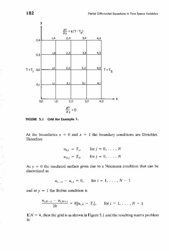
182
y
Partial Differential Equations in Two Space Variables
0,4
0,3
0,1
aT = k(T-T: )ay 2
1,4 2,4 3,4 4,4
13 23 3.3 43
12 22 32 42T=T2
II 21 31 41
0,0 1,0 2,0
aT =0ay
3,0 4,0x
FIGURE. 5. t Grid fOil" Example t.
At the boundaries xTherefore
°and x 1 the boundary conditions are Dirichlet.
for j = 0, ... ,N
for j = 0, ... ,N
At Y = °the insulated surface gives rise to a Neumann condition that can bediscretized as
and at y
Ui,-l - Ui,l = 0,
1 the Robin condition is
for i = 1, . . . , N - 1
Ui,N-l - Ui,N+l = k[. - T]2h U"N 2 , for i = 1, . . . , N - 1
If N = 4, then the grid is as shown inFigure 5.1 and the resulting matrix problemis:
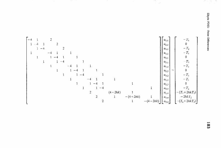
~
~n'"0,.."VI
I"T15'ii
-4 1 2 u1,o -T10
~1 -4 1 2 uz,o 0 ro
:J
1 -4 2 U3,O - TznroU>
1 -4 1 1 ul,l - T1
1 1 -4 1 1 UZ,l 01 1 -4 1 U 3,1 - Tz
1 -4 1 1 Ul,Z - T1
1 1 -4 1 1 uz,z = 01 1 -4 1 U3,Z - Tz
1 -4 1 1 u1,3 - T1
1 1 -4 1 1 UZ,3 01 1 -4 1 U3,3 -Tz
2 (4 +2hk) 1 Ul,4 - (T1 +2hkTz)
2 1 - (4+2hk) 1 UZ,4 -2hkTz
2 1 - (4 +2hk) U3,4 - (Tz+2hkTz )
-goW
j84 Partial Differential Equations in Two Space Variables
Notice how the boundary conditions are incorporated into the matrix problem.The matrix generated by the finite difference discretization is sparse, and anappropriate linear equation solver should be employed to determine the solution.Since the error is 0(h2 ), the error in the solution with N = 4 is 0(0.0625). Toobtain a smaller error, one must increase the value of N, which in turn increasesthe size of the matrix problem.
for (x, y) on aR
for (x, y) on aR
Variable Coefficients and Nonlinear Problems
Consider the following elliptic PDE:
- (P(x, y)wx)x - (P(x, y)wy)y + Tj(x, y)wo- = f(x, y)
defined on a region R with boundary aR and
awa(x, y)w + b(x, y) - = c(x, y),an
Assume that P, Px, Py, Tj, and f are continuous in Rand
P(x, y) > 0
Tj(x, y) > 0
Also, assume a, b, and c are piecewise continuous and
a(x, y) ;::", O}b(x, y) ;::",0a + b > 0
(5.13)
(5.14)
(5.15)
(5.16)
If (T = 1, then (5.13) is called a self-adjoint elliptic PDE because of the formof the derivative terms. A finite difference discretization of (5.13) for any interiornode is
-OxCP(x;, y)oxu;) - oiP(x;, yj)OyU;,j) + Tj(x;, y)ut,j = f(x;, Yj)
where
U;+1/2,j - U;-1/2,jo u· . = ----"------==""-x ',j ~x
U;,j+1/2 - U;,j-1/2OyU;,j = -"-'-'-'::'::-~-y-~-=-=
(5.17)
The resulting matrix problem will still remain in block-tridiagonal form, but if(T #. 0 or 1, then the system is nonlinear. Therefore, a Newton iteration mustbe performed. Since the matrix problem is of considerable magnitude, one wouldlike to minimize the number of Newton iterations to obtain solution. This is therationale behind the Newton-like methods of Bank and Rose [1]. Their methodstry to accelerate the convergence of the Newton method so as to minimize theamount of computational effort in obtaining solutions from large systems of
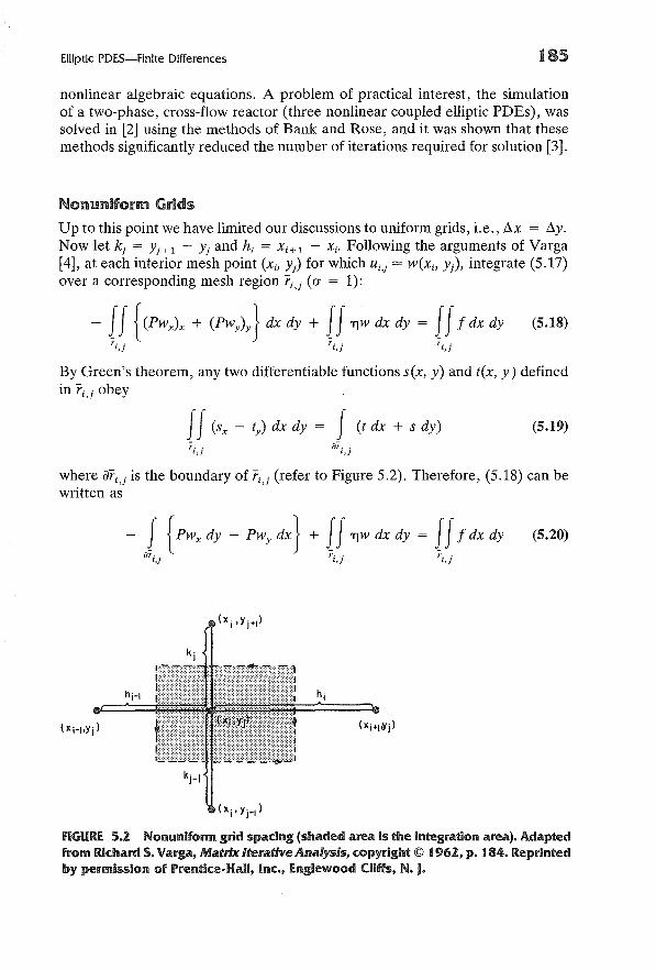
Elliptic PDES-Finite Differences 185
nonlinear algebraic equations. A problem of practical interest, the simulationof a two-phase, cross-flow reactor (three nonlinear coupled elliptic PDEs), wassolved in [2] using the methods of Bank and Rose, and it was shown that thesemethods significantly reduced the number of iterations required for solution [3].
Nonuniform Grids
Up to this point we have limited our discussions to uniform grids, i.e., Ax = Ay.Now let kj = yj+l - Yj and hi = Xi + 1 - Xi- Following the arguments of Varga[4], at each interior mesh point (Xi' y) for which Ui,j = w(xi, Yj), integrate (5.17)over a corresponding mesh region ri,j (a = 1):
(5.18)
By Green's theorem, any two differentiable functions sex, y) and t(x, y) definedin ri,j obey
JJ(sx - ty) dx dy = J (t dx + s dy)~. . ~..i,J I,]
(5.19)
where ari,j is the boundary of ri,j (refer to Figure 5.2). Therefore, (5.18) can bewritten as
(5.20)
hj-I hi
fiGURE 5.2 Nonuniform grid spacing (shaded area is the integration area). Adaptedfrom Richard S. Varga, Matrix Iterative Analysis, copyright © t 962, p. t 84. Reprintedby permission of Prentice-Hall, Inc., Englewood Cliffs, N. J.
186 Partial Differential Equations in Two Space Variables
The double integrals above can be approximated by
II z dx dy = A· . z· .1,J l,J
r ..loj
for any function z(x, y) such that z(x;, Yj) = Z;,j and
(h;-l + hJ(kj - 1 + k)A- . = -'-------'----'-
l,j 4
(5.21)
The line integral in (5.20) is approximated by central differences (integrationfollows arrows on Figure 5.2). For example, consider the portion of the lineintegral from (X;+l/2> Yj-lIz) to (Xi+lIZ' Yj+lIz):
where
Therefore, the complete line integral is approximated by
Using (5.23) and (5.21) on (5.20) gives
(5.22)
(5.23)
(5.24)
Elliptic PDES-Finite Differences
where
(h i - 1 + hi)(kj - 1 + kj )D'.,j. = L· . + M . + T· + B· . + 'n .. ------'----'-
I,j l,j I,j I,j 'Il,j 4
hi - 1 hik-T . = -- p. 1 ·+1 + -2 p'.+!,j.+!
j I,j 2 1- 2,j 2 2 2
181
Notice that if hi = hi - 1 = kj = kj - 1 and P(x, y) = constant, (5,24) becomesthe standard second-order accurate difference formula for (5.17). Also, noticethat if P(x, y) is discontinuous at Xi and/or Yj as in the case of inhomogeneousmedia, (5.24) is still applicable since P is not evaluated at either the horizontal(Yj) or the vertical (x;) plane. Therefore, the discretization of (5.18) at any interiornode is given by (5.24). To complete the discretization of (5.18) requires knowledge of the boundary discretization. This is discussed in the next section.
EXAMPLE 2
In Chapter 4 we discussed the annular bed reactor (see Figure 4.5) with its masscontinuity equation given by (4.46). If one now allows for axial dispersion ofmass, the mass balance for the annular bed reactor becomes
01at = [AmAn] L~ (rDrat) + [An/Am]~ (Dz at) + [AmAn] 02<tlR(f)az ReSc rar ar ReSc az az ReSc
where the notation is as in (4.46) except for
Dr = dimensionless radial dispersion coefficientDZ = dimensionless axial dispersion coefficient
At r = rsc> the core-screen interface, we assume that the convection term isequal to zero (zero velocity), thus reducing the continuity equation to
! i (rDr at) + ~ (Dz at) = 0rar ar az az
188 Partial Differential Equations in Two Space Variables
Also, since the plane r = rsc is an interface between two media, Dr and DZ arediscontinuous at this position. Set up the difference equation at the interfacer = rsc using the notation of Figure 5.3. If we now consider Dr and DZ to beconstants, and let hi- 1 = hi' and k j - 1 = k j , show that the interface discretizationsimplifies to the standard second-order correct discretization.
SOLUTION
Using (5.18) to discretize the PDE at r = rsc gives
-II [! i (rDr at) + ~ (Dz at)] r dr dz 0_ r ar ar az azr ..
'.}
Upon applying Green's theorem to this equation, we have
I [ at at]- rDr - dz - DZ - r dr = 0_ ar azar. .'.}
If the line integral is approximated by central differences, then
(h 1 h ) (u ..-U·· 1)+ ~Dz + -.!.Dz l,j I,j- - 0
. 1· 1 . 1· 1 r· -2 l-_,j-_ 2 l+-,j-_ 1 k
2 2 2 2 j-1
where
Di-l,j+l = Di-l,j-l = D~2 2 2 2
Df-£,j+£ = Df-l,j-l = D~2 2 2 2
Now if Dr and DZ are constants, hi- 1 hi = h, and k j - 1 = k j = k, a secondorder correct discretization of the continuity equation at r = rsc is
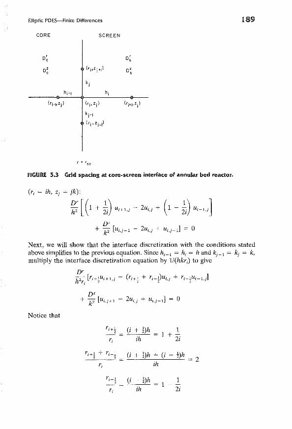
Elliptic PDES-Finite Differences 189
CORE SCREEN
(rj, Z j)
k j-I
(rj,zH)
r = rsc
FIGURE 5.3 Grid spacing at core-screen interface of annular bed reador.
(ri = ih, Zj = jk):
~: [(1 + ~) ui+1,j - 2ui,j + (1 - ~) U i - 1,j]
DZ+ k2 [Ui,j+1 - 2ui,j + Ui,j-1] = 0
Next, we will show that the interface discretization with the conditions statedabove simplifies to the previous equation. Since hi -1 = hi = hand kj -1 = kj = k,multiply the interface discretization equation by l/(hkri) to give
DZ+ k2 [Ui,j+1 - 2ui,j + ui,j-d 0
Notice that
ri+~ (i+ !)h 11 +-
r i ih 2i
ri+1 + ri-1 (i + !)h + (i - ~)h2 2 2r i ih
ri-1 (i - ~)h 12 1r i ih 2i
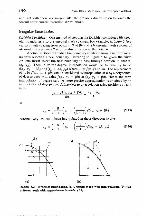
190 Partial Differential Equations in Two Space Variables
and that with these rearrangements, the previous discretization becomes thesecond-order correct discretion shown above.
Irregular Boundaries
Dirichlet Condition One method of treating the Dirichlet condition with irregular boundaries is to use unequal mesh spacings. For example, in figure SAa avertical mesh spacing from position B of f3h and a horizontal mesh spacing ofOI.h would incorporate aR into the discretization at the point B.
Another method of treating the boundary condition using a uniform meshinvolves selecting a new boundary. Referring to Figure SAa, given the curveaR, one might select the new boundary to pass through position B, that is,(xs, Ys)· Then, a zeroth-degree interpolation would be to take Us to bef(xs, Ys + f3h) or f(xs + OI.h, Ys) where w = f(x, y) on aR. The replacementof Us by f(xs, Ys + f3h) can be considered as interpolation at B by a polynomialof degree zero with value f(xs, Ys + f3h) at (xs, Ys + f3h). Hence the terminterpolation of degree zero. A more precise approximation is obtained by aninterpolation of degree one. A first-degree interpolation using positions Us andUc is:
Us - f(xs, Ys + f3h)f3h
or
Us = (f3 ~ l)UC + (f3 ~ l)f(xs, Ys + f3h)
Alternatively, we could have interpolated in the x-direction to give
Us = (01. : l)UA + (01. ~ l)f(xs + OI.h, Ys)
/3h
(5.25)
(5.26)
ilR
(0)
ilR
(b)
fiGURE 5.4 Irregular boundaries. (a) Uniform mesh with interpolation. (b) Nonuniform mesh with approximate boundary aRh'
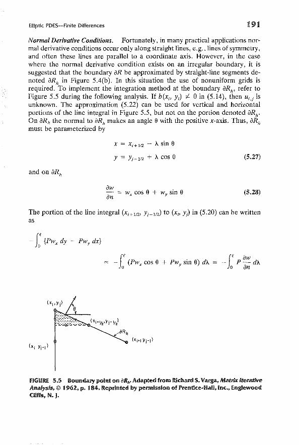
Elliptic PDES-Finite Differences 191
Normal Derivative Conditions. Fortunately, in many practical applications normal derivative conditions occur only along straight lines, e.g., lines of symmetry,and often these lines are parallel to a coordinate axis. However, in the casewhere the normal derivative condition exists on an irregular boundary, it issuggested that the boundary aR be approximated by straight-line segments denoted aRh in Figure 5.4(b). In this situation the use of nonuniform grids isrequired. To implement the integration method at the boundary aRh' refer toFigure 5.5 during the following analysis. If b(xi, yJ :;f 0 in (5.14), then Ui,j isunknown. The approximation (5.22) can be used for vertical and horizontalportions of the line integral in Figure 5.5, but not on the portion denoted aRh'On aRh the normal to aRh makes an angle ewith the positive x-axis. Thus, aRhmust be parameterized by
x = Xi+1/2 - 'A sin e
and on aRh
Y = Yj-1/2 + 'A cos e
aWe' e- = Wx cos + wy sman
(5.27)
(5.28)
The portion of the line integral (Xi+1/2' Yj-1/2) to (Xi' y) in (5.20) can be writtenas
if if aw- (PWx cos e + PWy sin e) d'A = - P- d'A
o 0 an
FIGURE 5.5 Boundary point on aRh' Adapted from Richard S. Varga, Matrix IteratIveAnalysIs, © 1962, p. 184. Reprinted by permission of Prentice-Hali, Inc., EnglewoodCliffs, N. J.
192 Partial Differential Equations in Two Space Variables
or by using (5.14):
-L{PWx dy - PWy dx} = - LP [C(A) -b~A~A)W(A)] dA
= _ p . . [Ci,j - ai,jUi,j] .e (5.29)',j b· .
t,j
where
1.e = - Yh2 + k?
2 ' r 1 (path length of integration).
Notice that we have used the boundary condition together with the differentialequation to obtain a difference equation for the point (x;, y).
ELLIPTIC PDES-fINITE ELEMENTS
Background
Let us begin by illustrating finite element methods with the following ellipticPDE:
and
a2W a2 w
-2 + -2 = -f(x, y),ax ay for (x, y) in R (5.30)
W(x, y) = 0, for (x, y) on aR (5.31)
Let the bounded domain R with boundary aR be the unit square, that is, 0 :;:::; x :;:::; 1,o< Y :;:::; 1. Finite element methods find a piecewise polynomial (pp) approximation, u(x, y), to the solution of (5.30). The pp-approximation can be writtenas
m
u(x, y) = La/pix, y)j=l
(5.32)
where {<hex, y)lj = 1, ... ,m} are specified functions that satisfy the boundaryconditions and {ajlj = 1, ... , m} are as yet unknown constants.
In the collocation method the set {ajlj = 1, , m} is determined bysatisfying the PDE exactly at m points, {(Xi' Yi)li = 1, , m}, the collocationpoints in the region. The collocation problem for (5.30) using (5.32) as the ppapproximation is given by:
ACa = -f (5.33)
Elliptic PDES-Finite Elements
where
193
f = [I(x!> Yl), ... ,f(xm, Ym)]T
The solution of (5.33) then yields the vector Ol, which determines the collocationapproximation.
To formulate the Galerkin method, first multiply (5.30) by <Pi and integrateover the unit square:
II e:~ + ~:~) <Pi dx dy = - II f(x, Y)<Pi dx dyR R
i = i, ... ,m
Green's first identity for a function t is
II (at a<pi at a<pi) d d--+-- x Yax ax ay ay
R
II (aZt aZt) I at= - - + - <p. dx dy + - <p. deaxz ayz I an I
R M
(5.34)
(5.35)
where
~ = denotes differentiation in the direction of outward normalan
e = path of integration for the line integral
Since the functions <Pi satisfy the boundary condition, each <Pi is zero on aR.Therefore, applying Green's first identity to (5.34) gives
II (aw a<Pi + aw a<pi) dx dy = II f(x, y) <Pi dx dyax ax ay ay
R R
i = 1, ... ,m
For any two piecewise continuous functions 1] and <\1 denote
(1], <\1) = II 1]<\1 dx dyR
(5.36)
(5.37)
Equation (5.36) can then be written as
(V'w, V'<Pi) = (f, <Pi)'where
i = 1, ... ,m (5.38)
V' = gradient operator.
194 Partial Differential Equations in Two Space Variables
This formulation of (5.30) is called the weak form. The Galerkin method consistsin finding u(x) such that
i = 1, ... ,m (5.39)
or in matrix notation,
where
g = [gl> ... ,gmV
gi = (I, <Pi)
Next, we discuss each of these methods in further detail.
(5.40)
CollocationIn Chapter 3 we outlined the collocation procedure for BVPs and found thatone of the major considerations in implementing the method was the choice ofthe approximating space. This consideration is equally important when solvingPDEs (with the added complication of another spatial direction). The moststraightforward generalization of the basis functions from one to two spatialdimensions is obtained by considering tensor products of the basis functions forthe one-dimensional space !L?k(1T) (see Chapter 3). To describe these piecewisepolynomial functions let the region R be a rectangle with G1 ~ x ~ bv Gz ~ Y ~ b2J
where -00 < Gi ~ bi < 00 for i = 1,2. Using this region Birkhoff et al. [5] andlater Bramble and Hilbert [6,7] established and generalized interpolation resultsfor tensor products of piecewise Hermite polynomials in two space variables.To describe their results, let
(5.41)
h = max hi = max (X i + 1 - xJl~is.;;.Nx l:s:i~Nx
k = max k· = max (Yj+l - Yj)l,,;,j,,;,Ny J l,,;,j,,;,Ny
p = max {hJ k}
be the partitions in the x- and y-directions, and set 1T = 1Tl X 1T2' Denote byQ32(1T) the set of all real valued piecewise polynomial functions <Pi defined on
1T such that on each subrectangle [XiJ Xi+l] x [YjJ Yj+d of R defined by 1T, <Pi isa polynomial of degree at most 3 in each variable (x or y). Also, each <Pi'
Elliptic PDES-finite Elements 195
(a<p;)/(ax), and (a<p;)/(ay) must be piecewise continuous. A basis for !Z!2 is thetensor products of the Hermite cubic basis given in Chapter 3 and is
{V;(X)Vj(y), s;(x)Vj(Y)' v;(x)s/y), S;(X)Sj(Y)} [:1 [:1 (5.42)
where the v's and s's are listed in Table 3.2. If the basis is to satisfy the homogeneous Dirichlet conditions, then it can be written as:
i = 1,Nx + 1, j = 1, ... ,Ny + 1i=1, ,Nx +1, j=1,Ny +1i = 2, ,Nx , j = 2, ... ,Ny
(5.43)
Using this basis, Prenter and Russell [8] write the pp-approximation as:
Nx +1 N y +1 [ auu(x, y) = 2: 2: u(xb Yj)v;Vj + - (x;, Yj)S;Vj
;=1 j=1 ax (5.44)
au a2u ]+ - (x;, Y)V;Sj + -- (x;, Yj)S;Sjay ax ay
which involves 4(Nx + 1)(Ny + 1) unknown coefficients. On each subrectangle[x;, x;+d X [Yj' Yj+d there are four collocation points that are the combinationof the two Gaussian points in the x direction, and the two Gaussian points inthe Y direction, and are:
TL = (x; + ~ [1 - ~l Yj + 1[1- ~])
TT,j = (x; + ~ [1 + ~l Yj + 1[1-~])TL = (x; + ~ [1 - ~l Yj + 1[1+ ~])
Ttj = (x; + ~ [1 + ~l Yj + 1[1+ ~])
(5.45)
Collocating at these points gives 4Nx Ny equations. The remaining 4Nx + 4Ny + 4equations required to determine the unknown coefficients are supplied by theboundary conditions [37]. To obtain the boundary equations on the sides x = a1
and x = h1 differentiate the boundary conditions with respect to y. For example,if
au = y2 at x = a1 and x = h1ax
196
then
Partial Differential Equations in Two Space Variables
(5.46)
a2 u-- = 2y at x = a l and x = b Iax ay
Equation (5.46) applied at Ny - 1 boundary nodes (yjlj = 2, ... , Ny) gives:
auax (a v Yj) = yJ
a2uax ay (aI' y) = 2Yj
auax (b v Yj) = yJ
(5.47)
or 4Ny - 4 equations. A similar procedure at y = a2 and y = b2 is followed togive 4Nx - 4 equations. At each corner both of the above procedures are applied.For example, if
(5.48)
then
au ag- (av a2) = - (aI' a2)ay ay
Thus, the four corners supply the final 12 equations necessary to completelyspecify the unknown coefficients of (5.44).
EXAMPLE 3
Set up the colocation matrix problem for the PDE:
a2 w a2w- + - = <P °~ x ~ 1, °~ Y ~ 1ax2 ay2 '
with
w = 0, for x = 1
w= 0, for y = 1
aw0, for x = °-=
ax
aw0, for y = °-=
ay
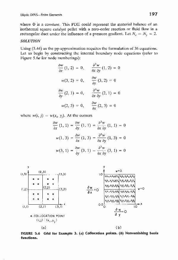
Elliptic DPES-Finite Elements 197
where 1> is a constant. This PDE could represent the material balance of anisothermal square catalyst pellet with a zero-order reaction or fluid flow in arectangular duct under the influence of a pressure gradient. Let N x = Ny = 2.
SOLUTION
Using (5.44) as the pp-approximation requires the formulation of 36 equations.Let us begin by constructing the internal boundary node equations (refer toFigure 5.6a for node numberings):
aw (1, 2) = 0, a2w (1, 2)
ax ax ay
w(3,2)aw
0, ay (3,2) = 0
~; (2, 1) 0,a2 w-(2 1)ax ay ,
w(2, 3) = 0, aw (2, 3) 0ax
o
o
where w(i, j) w(x i, yJ At the corners
aw (1, 1) = aw (1, 1) = a2
w (1, 1) 0ax ay ax ay
aw a2 ww(l, 3) = - (1, 3) = - (1, 3) 0
ax ax ay
w(3,1) aw (3, 1) = a2
w (3, 1) 0ay ax ay
y y
,3)
(1,1)x
=0
1.0
~=oo y
w=O
V1V2 ,VI SZi'I S3 V2VZtV2SZ,V2S3
V2V2 ,V252/253 S2V2,5{>2,5253
S2V2'5252~2S, 5,v2,5?2'S3%w
VI VI' VI V2,VI~ V2V1,V2V2 ,V2~
v2v[ 1 V2V2,V2S; 52V,,52V2 ,5,A,
5 2V"S2V2'Sij, 53V,,53V2,~
1.0
ow =0ax
,2)
x(2,1) (3,1)
EI:COLLOCATION POINT
(i,j) : (x i' Yj )
(2,3)(3
EI EI EI EI
EI EI EI EI
(2,2) (3EI EI EI EI
EI EI EI EI
(1,2)
(1,3)
(0) (b)
fiGURE. 5.6 Grid for Example 3. (a) Collocation points. (b) Nonvanishing basisfunctions.
198
and
Partial Differential Equations in Two Space Variables
aw aww(3, 3) = - (3, 3) = - (3, 3) = 0
ax ay
This leaves 16 equations to be specified. The remaining 16 equations are thecollocation equations, four per subrectangle (see Figure 5.6a). If the aboveequations involving the boundary are incorporated in the pp-approximation,then the result is
U(x, y)
a=
where
U;,j = u(x;, Yj)
The pp-approximation is then used to collocate at the 16 collocation points.Since the basis is local, various terms of the above pp-approximation can bezero at a given collocation point. The nonvanishing terms of the pp-approximation are given in the appropriate subrectangle in Figure 5.6b. Collocating atthe 16 collocation points using the pp-approximation listed above gives thefollowing matrix problem:
where
1 = [1, ... , IV
[aUl Z aU13 auz 1
U U --'--'U --'UI,V I,Z' ay' ay' Z,V ax' z,z
auz,z auz,z aZuz,z aUZ,3 aZUZ,3ax' ay' ax ay' ay' ax ay
aU3,1 au3,z aZu3,z aZU3,3]Tax' ax' ax ay' ax ay
(for any function 1jJ)
and for the matrix A c,
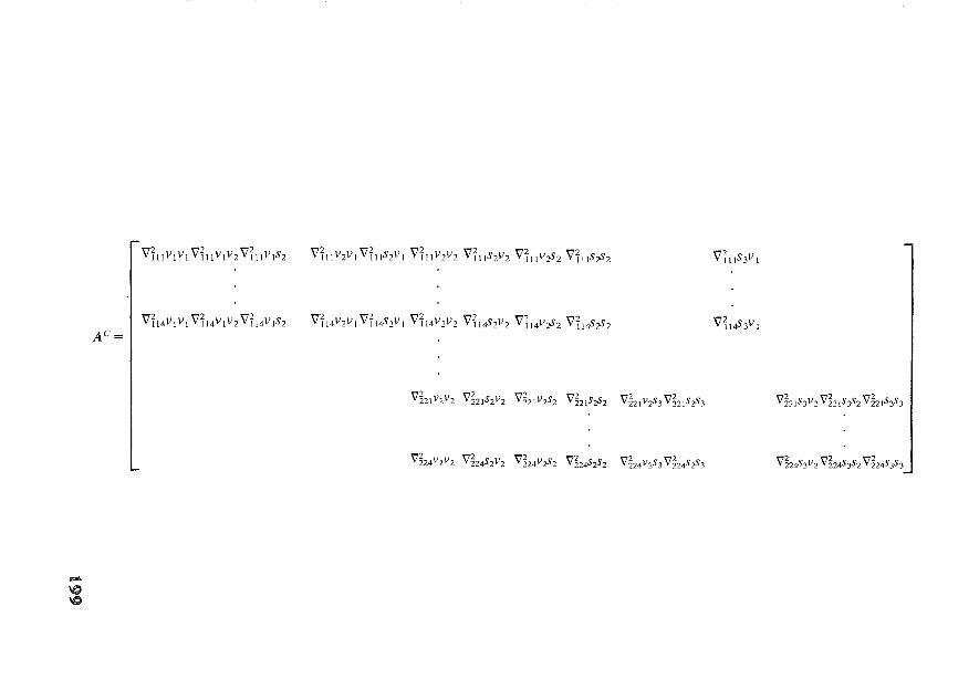
-\C\C
A C =
V'IIIV1V 1V'IIIVlVZ V'I11V1SZ
V'II4VI Vl V'II4V I VZV'II4VlSZ
V'I11VZV 1V'I11SZV 1 V'IIIVZVZ V'Il1SZVZ V'I11VzSZ V'I11SzSZ
V'II4VZVl V'II4SZV l V'II4VZVZ V'II4S ZVZ V'II4VzSZ V'II4S zSZ
V'~ZIV2V2 V'~ZISZVZ V'~21VZSZ V'bszsz V'~ZIVZS3V'bSZS3
V'~Z4VZVZ V'~Z4SZVZ V'~Z4VZSZ V'~Z4S2SZ V'~Z4VZS3V'~Z4SZS3
V'11IS 3V 1
V'114S 3V :
V'~21S3VZ V'~ZIS3SZ V'bS3S3
V'~24S3V ZV'~Z4S3S2 V'~Z4S3S3
200 Partial Differential Equations in Two Space Variables
The solution of this matrix problem yields the vector a, which specifies the valuesof the function and its derivatives at the grid points.
Thus far we have discussed the construction of the collocation matrix problem using the tensor products of the Hermite cubic basis for a linear PDE. Ifone were to solve a nonlinear PDE using this basis, the procedure would be thesame as outlined above, but the ensuing matrix problem would be nonlinear.
In Chapter 3 we saw that the expected error in the pp-approximation whensolving BVPs for ODEs was dependent upon the choice of the approximatingspace, and for the Hermite cubic space, was O(h4). This analysis can be extendedto PDEs in two spatial dimensions with the result that [8]:
lu(x, y) - w(x, y)1 = O(p4)
Next, consider the tensor product basis for.!Z!'fe ('ITl) x .!Z!'fe ('ITz) where 'ITI andx y
'ITz are given in (5.41), kx is the order of the one-dimensional approximatingspace in the x-direction, and ky is the order of the one-dimensional approximatingspace in the y-direction. A basis for this space is given by the tensor productsof the B-splines as:
/
DIMX IDIMY
B;(x)B~(y) i~l j~l
where
Bf(x) = B-spline in the x-direction of order kx
B~(y) = B-spline in the y-direction or order ky
DIMX = dimension of .!Z!t
DIMY = dimension of .!Z! 'fey
The pp-approximation for this space is given by
DIMX DIMY
u(x, y) = 2: 2: (Xi,jBf(x)B~(y)i~ 1 j= 1
where (Xi,j are constants, with the result that
lu(x, y) - w(x, y)1 = O(p'!)
where
(5.49)
(5.50)
(5.51)
Galerkin
The literature on the use of Galerkin-type methods for the solution of ellipticPDEs is rather extensive and is continually expanding. The reason for this growthin use is related to the ease with which the method accommodates complicated
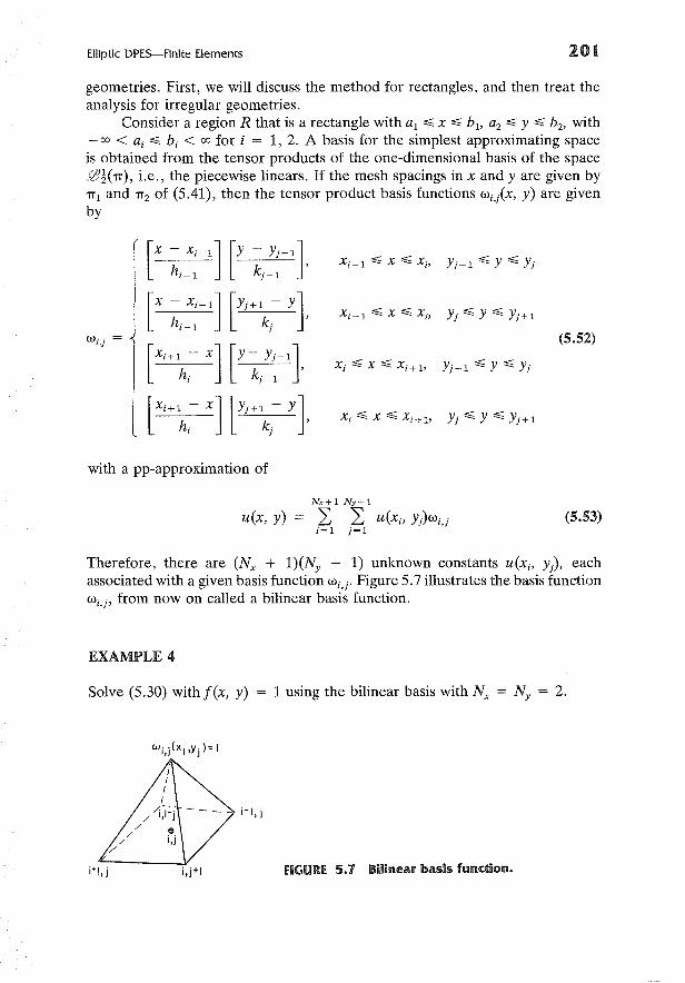
Elliptic DPES-Finite Elements 201
geometries. First, we will discuss the method for rectangles, and then treat theanalysis for irregular geometries.
Consider a region R that is a rectangle with a l ~ x ~ bl , a2 ~ Y ~ b2, with-00 < ai ~ bi < 00 for i = 1,2. A basis for the simplest approximating spaceis obtained from the tensor products of the one-dimensional basis of the space..0i(1T), i.e., the piecewise linears. If the mesh spacings in x and yare given by1TI and 1T2 of (5.41), then the tensor product basis functions wi,/x, y) are givenby
[x - Xi-I] [Y - Yj-ll Xi- l ~ x~ Xi' Yj-l ~ Y ~ Yjhi- l kj- l
[X - Xi-I] [Yj+l - Y1 Xi- l ~ X ~ Xi' Yj~Y ~Yj+lhi- l kj
Wi,j (5.52)
[Xi+l - X] [Y-Yj-l} Xi~X~Xi+h Yj-l ~ Y ~ Yjh, k j - l
[Xi+lhi- X] [Yj+lkj- Y1 Xi ~ X ~ Xi+h Yj~Y~Yj+1
with a pp-approximation of
Nx+l Ny+lu(x, y) = L L U(Xi' Yj)Wi,j
i= I j= I(5.53)
Therefore, there are (Nx + l)(Ny + 1) unknown constants u(xi , y), eachassociated with a given basis function Wi,j' Figure 5.7 illustrates the basis functionWi,j' from now on called a bilinear basis function.
EXAMPLE 4
Solve (5.30) with f(x, y) 1 using the bilinear basis with Nx = Ny = 2.
fiGURE 5.7 Bilinear basis function.
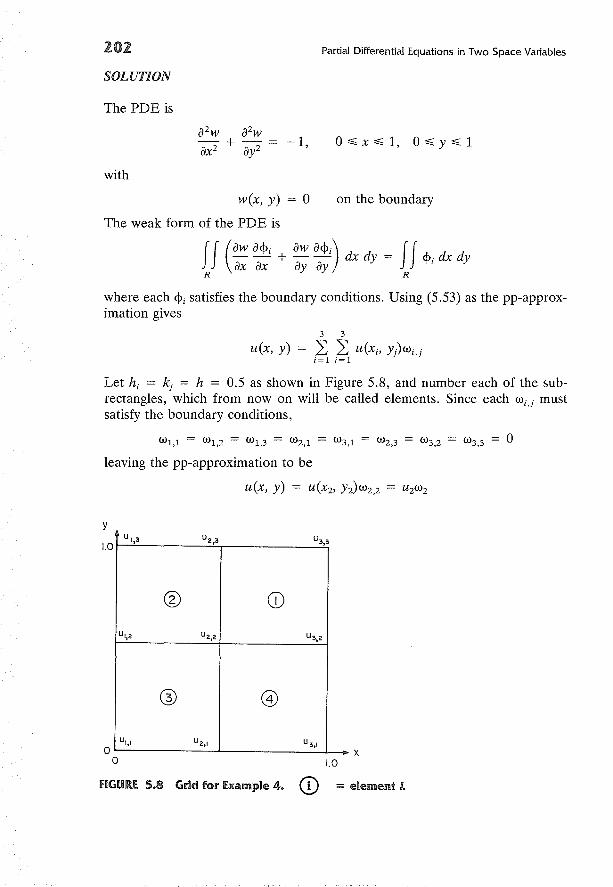
202 Partial Differential Equations in Two Space Variables
SOLUTION
The PDE is
0<;; x <;; 1, 0 <;; Y <;; 1
with
w(x, y)
The weak form of the PDE is
o on the boundary
II (aw a<Pi aw a<pi) II- -- + - -- dx dy = <Pi dx dyax ax ay ay
R R
where each <Pi satisfies the boundary conditions. Using (5.53) as the pp-approximation gives
3 3
u(x, y) = 2: 2: u(xi, Yj)Wi,ji~ 1 j~ 1
Let hi = k j = h = 0.5 as shown in Figure 5.8, and number each of the subrectangles, which from now on will be called elements. Since each Wi,j mustsatisfy the boundary conditions,
leaving the pp-approximation to be
u(x, y) = u(xz, yz)wz,z = UzWz
y
x1.0
U 1,3 U 2 ,3 U 3,3
® CDU 1,2 U2,2 U 3,2
® @
U',I U 2tl U 3,Ioo
1.0
fiGURE 5.8 Grid for Example 4. CD = element I.
Elliptic DPES-Finite Elements 203
Therefore, upon substituting u(x, y) for w(x, y), the weak form of the PDEbecomes
II ( awz awz awz awz) IIUz - - + Uz - - dx dy = Wz dx dyax ax ay ay
R R
or
where
II (awz awz + awz awz) dx dAzz = ax ax ay ay y
R
gz = II Wz dx dyR
This equation can be solved on a single element ei as
ei = 1, ... ,4
and then summed over all the elements to give
4 4
Azzuz = L A~2UZ = L g~; = gzei=l ej=l
In element 1:
Uzu(x, y) = hZ (1 - x)(l - y),
and
0.5 ~ x ~ 1, 0.5 ~ Y ~ 1
1W z = hZ (1 - x)(l - y)
Thus
Aiz = h14 e e [(1 - yf + (1 - x)Z] dx dy = ~)0.5 )0.5 3
and
gi = 1z f e (1 - x)(l - y) dx dy = hZ
h 0.5 )0.5 4
For element 2:
(h = 0.5)
Uzu(x, y) = hZ (1 - y)x, o~ x ~ 0.5, 0.5 ~ Y ~ 1.0
204
and
giving
and
Partial Differential Equations in Two Space Variables
1W z = hZ x(l - Y)
The results for each element are
Element Aei22
12'3
2 23
3 :<3
4 23
Thus, the solution is given by the sum of these results and is
Uz = i hZ = 0.09375
In the previous example we saw how the weak form of the PDE could besolved element by element. When using the bilinear basis the expected error inthe pp-approximation is
Iu(x, Y) - w(x, Y)I = O(pZ) (5.54)
(5.55)
where p is given in (5.41). As with ODEs, to increase the order of accuracy,the order of the tensor product basis functions must be increased, for example,the tensor product basis using Hermite cubics given an error of 0(p4). To illustratethe formulation of the Galerkin method using higher-order basis functions, letthe pp-approximation be given by (5.50) and reconsider (5.30) as the ellipticPDE. Equation (5.39) becomes
(V ~~x ~~y (Xi,jB~(x)B;(y), VB;';,(X)B~(Y)) = 0B;';,(X)B~(Y))
m = 1, ... , DIMX, n = 1, ... , DIMY
In matrix notation (5.55) is
Aa = g (5.56)
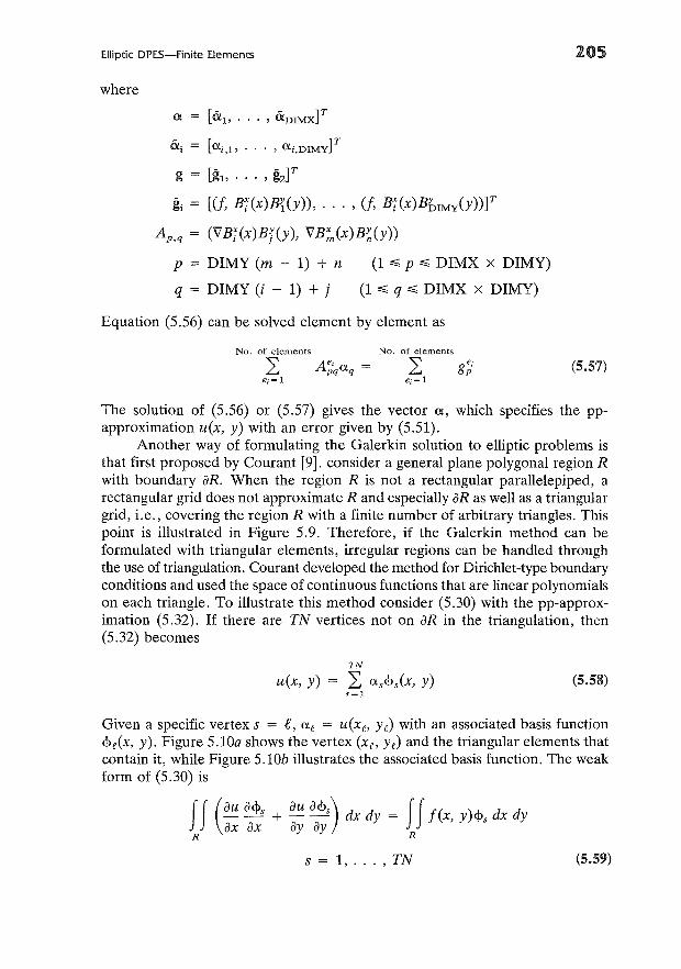
Elliptic DPES-Finite Elements
where
_ [- - ]Tg - gl>"" gz
gj = [(f, B:(x)B{(y)), ... , (f, B:(x)Bt>IMy(y))]T
Ap,q = (VB:(x)Br(y), VB~,(x)B~(y))
p = DIMY (m - 1) + n (1 ~ P ~ DIMX x DIMY)
q = DIMY (i - 1) + j (1 ~ q ~ DIMX x DIMY)
Equation (5.56) can be solved element by element as
No. of elements No. of elements
L Aiq<Xq = L giei=l ei=l
205
(5.57)
The solution of (5.56) or (5.57) gives the vector a, which specifies the ppapproximation u(x, y) with an error given by (5.51).
Another way of formulating the Galerkin solution to elliptic problems isthat first proposed by Courant [9]. consider a general plane polygonal region Rwith boundary aR. When the region R is not a rectangular parallelepiped, arectangular grid does not approximate R and especially aR as well as a triangulargrid, i.e., covering the region R with a finite number of arbitrary triangles. Thispoint is illustrated in Figure 5.9. Therefore, if the Galerkin method can beformulated with triangular elements, irregular regions can be handled throughthe use of triangulation. Courant developed the method for Dirichlet-type boundaryconditions and used the space of continuous functions that are linear polynomialson each triangle. To illustrate this method consider (5.30) with the pp-approximation (5.32). If there are TN vertices not on aR in the triangulation, then(5.32) becomes
TN
u(x, y) = L <Xs<Ps(x, y)s~l
(5.58)
Given a specific vertex s = e, <Xe = u(xf, Ye) with an associated basis function<l>e(x, y). Figure 5.lOa shows the vertex (xeo Ye) and the triangular elements thatcontain it, while Figure 5.10b illustrates the associated basis function. The weakform of (5.30) is
II (au a<l>s + au a<l>s) dx dy = II f(x, Y)<l>s dx dyax ax ay ay
R R
s = 1, ... , TN (5.59)
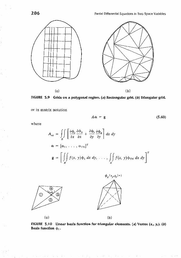
206
(0)
Partial Differential Equations in Two Space Variables
(b)
fiGURE 5.9 Grids on a polygonal region. (a) Rectangular grid. (b) Triangular grid.
or in matrix notation
Aa = g
where
A sq = JJ [a<ps a<pq + a<ps a<pq] dx dyax ax ay ay
R
g = [JJf(x, Y)<Pl dx dy, ... , JJf(x, y)<PTN dx dY] T
R R
(5.60)
(0) (b)
fiGURE 5.10 Linear basis function for triangular elements. (a) Vertex (xe, Ye)' (b)Basis function <Pe.
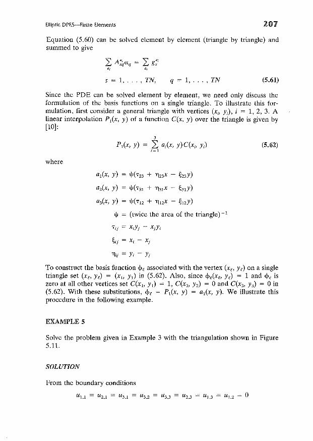
Elliptic DPES-Finite Elements 207
Equation (5.60) can be solved element by element (triangle by triangle) andsummed to give
2: A;~aq = 2: g;iei ej
s = 1, ... , TN, q = 1, ... , TN (5.61)
Since the PDE can be solved element by element, we need only discuss theformulation of the basis functions on a single triangle. To illustrate this formulation, first consider a general triangle with vertices (Xi' Yi), i = 1, 2, 3. Alinear interpolation Pl(x, y) of a function C(x, y) over the triangle is given by[10]:
where
3
Pl(x, y) = 2: a;(x, Y)C(Xb y;)i=l
al(x, y) = l/J(-r23 + 'll23X - ~23Y)
a2(x, y) = l/J(-r3l + 'll3lX - ~3lY)
a3(x, y) = l/J(T12 + 'll12X - ~12Y)
l/J = (twice the area of the triangle)-l
(5.62)
To construct the basis function <Pe associated with the vertex (xe, Ye) on a singletriangle set (xe, Ye) = (Xl, Yl) in (5.62). Also, since <Pe(xe> Ye) = 1 and <Pe iszero at all other vertices set C(xl, Yl) = 1, C(x2, Y2) = 0 and C(X3' Y3) = 0 in(5.62). With these substitutions, <Pe = PI(X, y) = al(x, y). We illustrate thisprocedure in the following example.
EXAMPLE 5
Solve the problem given in Example 3 with the triangulation shown in Figure5.11.
SOLUTION
From the boundary conditions
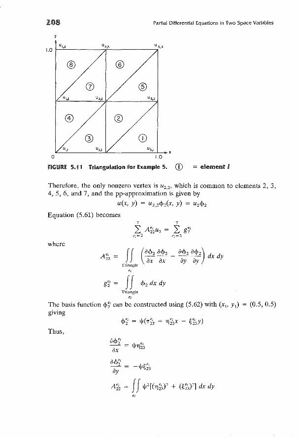
208 Partial Differential Equations in Two Space Variables
y
1.0U 1,3 U 2,3 U 3,3
® ®
CD ®U 1,2 U 2,2 U 3,2
@) ®
® CDU 2,I U 3,I
X
0 1.0
fiGURE 5.11 Triangulation for Example 5. CD = element J
Therefore, the only nonzero vertex is uz,z, which is common to elements 2, 3,4, 5, 6, and 7, and the pp-approximation is given by
u(x, y) = uz,z<Pz(x, y) = uz<Pz
Equation (5.61) becomes7 7
~ A~2Uz = ~ g~iei=2 ei=2
where
A ei = JJ (a<pz a<pz + a<pz a<pz) dx dzz ax ax ay ay y
Triangleei
Triangleei
The basis function <p~i can be constructed using (5.62) with (Xl> Yl) = (0.5,0.5)giving
Thus,
e,
Elliptic DPES-Finite Elements
and
ei
For element 2 we have the vertices
(Xl' Yl) = (0.5, 0.5)
(X2' Y2) = (1, 0.5)
(x3 , Y3) = (0.5, 0)
and
1tV = 0.25
1"23 = (1)(0) - (0.5)(0.5) = - 0.25
~23 = 1 - 0.5 = 0.5
1123 = 0.5
A~2 = II (0.25)-2[(0.5)2 + (0.5)2] dx dy = 1
2 - II 1 ] _ 0.25g2 - (0.25) [-0.25 + 0.5x - 0.5y dx dy - -6-
Likewise, the results for other elements are
Element Aei g;i22
0.252 1.0 -
6
0.50.25
3 -6
0.50.25
4 -6
0.255 0.5 -
6
0.50.25
6 -6
0.257 1.0 -
6-
Total 4.0 0.25
which gives
U2 = 0.0625
209
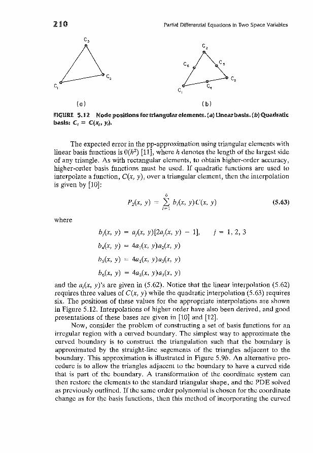
210
C3
Partial Differential Equations in Two Space Variables
c,
(a)
C2
( b)
fiGURE 5. t 2. Node positions for triangular elements. (a) Linear basis. (b) Quadraticbasis: C, = C(x" y,).
The expected error in the pp-approximation using triangular elements withlinear basis functions is O(h2
) [11], where h denotes the length of the largest sideof any triangle. As with rectangular elements, to obtain higher-order accuracy,higher-order basis functions must be used. If quadratic functions are used tointerpolate a function, C(x, Y), over a triangular element, then the interpolationis given by [10]:
where
6
L bi(x, y)C(x, y)i= 1
(5.63)
j = 1, 2, 3b/x, y) = aj(x, y)[2aj(x, y) - 1],
b4(x, y) = 4a1(x, y)a2(x, y)
bs(x, y) = 4a 1(x, y)a3(x, y)
b6(x, y) = 4aix, y)a3(x, y)
and the ai(x, y)'s are given in (5.62). Notice that the linear interpolation (5.62)requires three values of C(x, y) while the quadratic interpolation (5.63) requiressix. The positions of these values for the appropriate interpolations are shownin Figure 5.12. Interpolations of higher order have also been derived, and goodpresentations of these bases are given in [10] and [12].
Now, consider the problem of constructing a set of basis functions for anirregular region with a curved boundary. The simplest way to approximate thecurved boundary is to construct the triangulation such that the boundary isapproximated by the straight-line segements of the triangles adjacent to theboundary. This approximation is illustrated in Figure 5.9b. An alternative procedure is to allow the triangles adjacent to the boundary to have a curved sidethat is part of the boundary. A transformation of the coordinate system canthen restore the elements to the standard triangular shape, and the PDE solvedas previously outlined. If the same order polynomial is chosen for the coordinatechange as for the basis functions, then this method of incorporating the curved
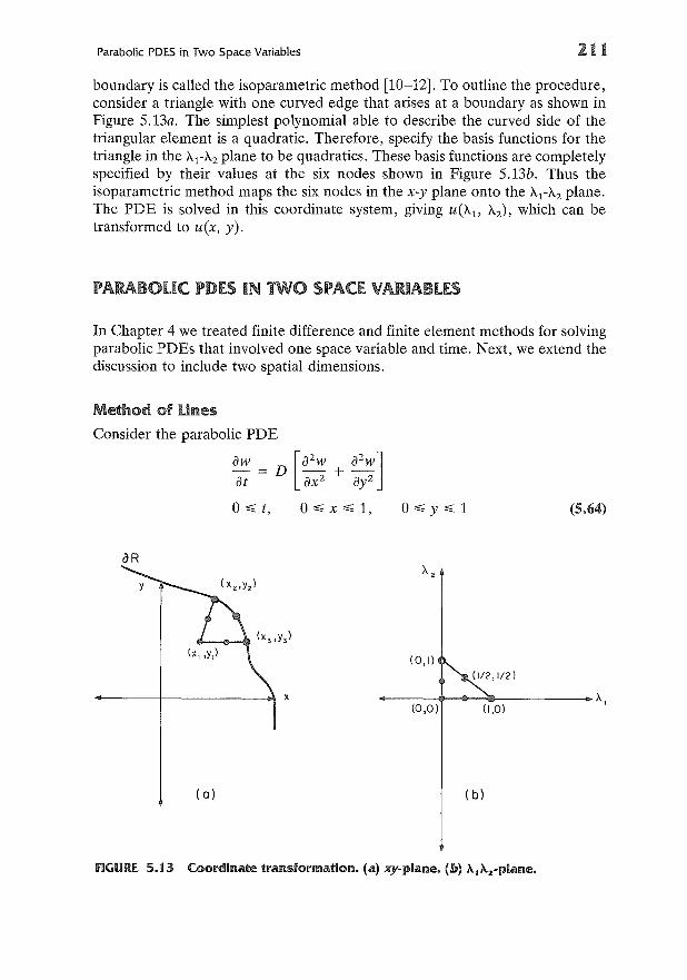
Parabolic PDES in Two Space Variables 211
boundary is called the isoparametric method [10-12]. To outline the procedure,consider a triangle with one curved edge that arises at a boundary as shown inFigure 5.13a. The simplest polynomial able to describe the curved side of thetriangular element is a quadratic. Therefore, specify the basis functions for thetriangle in the Al-A2 plane to be quadratics. These basis functions are completelyspecified by their values at the six nodes shown in Figure 5.13b. Thus theisoparametric method maps the six nodes in the x-y plane onto the ACA2 plane.The PDE is solved in this coordinate system, giving U(Al> A2), which can betransformed to u(x, y).
PARABOLIC PDES IN TWO SPACE VARIABLES
In Chapter 4 we treated finite difference and finite element methods for solvingparabolic PDEs that involved one space variable and time. Next, we extend thediscussion to include two spatial dimensions.
Method of Lines
Consider the parabolic PDE
aw = D [a 2 w + a2 w]at ax2 ay2
oR
o~ t, o~ x ~ 1, (5.64)
( 0)
(O,I)
-----...~II--....-----... },.,(0,0) (1,0)
( b)
fiGURE. 5.13 C.oordinate transformation. (a) xy-plane. (b) AtAz-plane.
212 Partial Differential Equations in Two Space Variables
(5.65)
with D constant. Discretize the spatial derivatives in (5.64) using finite dif-ferences to obtain the following system of ordinary differential equations:
au·· D Da~'J = (LiX)JUi+1,j - 2ui,j + Ui-1J + (Liy)JUi,j+l - 2ui,j + Ui,j-l]
where
Ui,j = w(xiJ y)
Xi = i Lix
Yj = j Liy
Equation (5.65) is the two-dimensional analog of (4.6) and can be solved in asimilar manner. To complete the formulation requires knowledge of the subsidiary conditions. The parabolic PDE (5.64) requires boundary conditions at X = 0,x = 1, y = 0, and y = 1, and an initial condition at t = 0. As with the MOLin one spatial dimension, the two-dimensional problem incorporates the boundary conditions into the spatial discretizations while the initial condition is usedto start the IVP.
Alternatively, (5.64) could be discretized using Galerkin's method or bycollocation. For example, if (5.32) is used as the pp-approximation, then thecollocation MOL discretization is
(5.66)
i = 1, ... ,m
where (Xi> y;) designates the position of the ith collocation point. Since the MOLwas discussed in detail in Chapter 4 and since the multidimensional analogs arestraightforward extensions of the one-dimensional cases, no rigorous presentation of this technique will be given.
Alternating Direction Implicit Methods
Discretize (5.65) in time using Euler's method to give
ut,j = [~~~] [U?+l,j + U?-l,j] + [~~;] [Ui,j+l + Ui,j-l]
[2D Lit 2D Lit]
+ ui,j 1 - (LiX)2 - (Liy)Z
where
(5.67)
Parabolic PDES in Two Space Variables
For stability
[ 1 1] 1D ilt (ilX)2 + (ily)2 < 2"
If ilx = ily, then (5.68) becomes
D ilt 1--~
(ilX)2 4
213
(5.68)
(5.69)
(5.70)
which says that the restriction on the time step-size is half as large as the onedimensional analog. Thus the stable time step-size decreases with increasingdimensionality. Because of the poor stability properties common to explicitdifference methods, they are rarely used to solve multidimensional problems.Inplicit methods with their superior stability properties could be used instead ofexplicit formulas, but the resulting matrix problems are not easily solved. Another approach to the solution of multidimensional problems is to use alternatingdirection implicit (ADI) methods, which are two-step methods involving thesolution of tridiagonal sets of equations (using finite difference discretizations)along lines parallel to the x-y axes at the first-second steps, respectively.
Consider (5.64) with D = 1 where the region to be examined in (x, y, t)space is covered by a rectilinear grid with sides parallel to the axes, andh = ilx = ily. The grid points (Xi' yj' tn ) given by x = ih, Y = jh, and t = n ilt,and ui,j is the function satisfying the finite difference equation at the grid points.Define
iltT = h2
Essentially, the principle is to employ two difference equations that are used inturn over successive time-steps of ilt/2. The first equation is implicit in the xdirection, while the second is implicit in the y-direction. Thus, if Ui,j is an intermediate value at the end of the first time-step, then
or
Ui,j un. T [ 2- + O~Ui,J= 2" °XUi,jl,J
Un+ 1 U· . T [ 2- + 02Un+l]= 2" °xUi,jl,J l,J Y l,J
[1 - ! Tonti = [1 + ! TO~]Un
[1 - !To~]Un+l = [1 + !Tonti
(5.71)
(5.72)
214
where
Partial Differential Equations in Two Space Variables
for all i and j
These formulas were first introduced by Peaceman and Rachford [13], andproduce an approximate solution which has an associated error of O(Lit2 + h2 ).
A higher-accuracy split formula is due to Fairweather and Mitchell [14] and is
[1 - H,. - ~) 8;]ii = [1 + H,. + ~) 8~]un
[1 - ~ (,. - ~) 8~]un+l = [1 + ~ (,. + ~) 8~]ii (5.73)
with an error of O(Llt2 + h4). Both of these methods are unconditionally stable.A general discussion of ADI methods is given by Douglas and Gunn [15].
The intermediate value ii introduced in each ADI method is not necessarilyan approximation to the solution at any time level. As a result, the boundaryvalues at the intermediate level must be chosen with care. If
W(x, y, t) = g(x, y, t) (5.74)
when (x, y, t) is on the bounadry of the region for which (5.64) is specified,then for (5.72)
and for (5.73)
Ui,j = ,. ~ ~ [1 - HT - n8~]gZ:1 + ,. ; ~ [1 + HT + ~) 8~]gi,j
(5.75)
(5.76)
If g is not dependent on time, then
Ui,j = gi,j (for 5.72) (5.77)
Ui,j = (1 + ~ 8~)gi,j (for 5.73) (5.78)
A more detailed investigation of intermediate boundary values in ADI methodsis given in Fairweather and Mitchell [16].
ADI methods have also been developed for finite element methods. Douglas and Dupont [17] formulated ADI methods for parabolic problems usingGalerkin methods, as did Dendy and Fairweather [18]. The discussion of thesemethods is beyond the scope of this text, and the interested reader is referredto Chapter 6 of [11].
MATHEMATICAL SOFTWARE
As with software for the solution of parabolic PDEs in one space variable andtime, the software for solving multidimensional parabolic PDEs uses the methodof lines. Thus a computer algorithm for multidimensional parabolic PDEs based
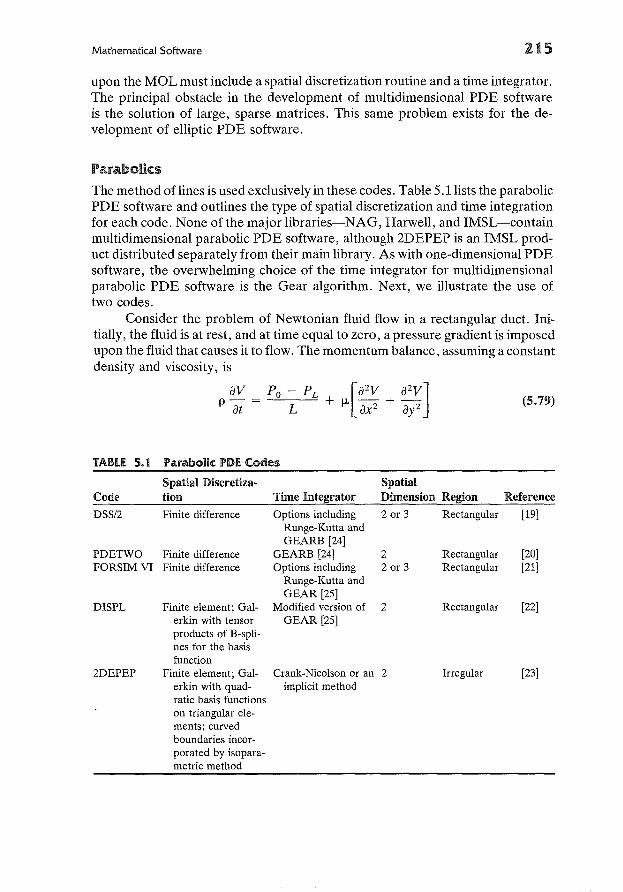
Mathematical Software 215
(5.79)
upon the MOL must include a spatial discretization routine and a time integrator.The principal obstacle in the development of multidimensional PDE softwareis the solution of large, sparse matrices. This same problem exists for the development of elliptic PDE software.
ParabolicsThe method of lines is used exclusively in these codes. Table 5.1 lists the parabolicPDE software and outlines the type of spatial discretization and time integrationfor each code. None of the major libraries-NAG, Harwell, and IMSL-containmultidimensional parabolic PDE software, although 2DEPEP is an IMSL product distributed separately from their main library. As with one-dimensional PDEsoftware, the overwhelming choice of the time integrator for multidimensionalparabolic PDE software is the Gear algorithm. Next, we illustrate the use oftwo codes.
Consider the problem of Newtonian fluid flow in a rectangular duct. Initially, the fluid is at rest, and at time equal to zero, a pressure gradient is imposedupon the fluid that causes it to flow. The momentum balance, assuming a constantdensity and viscosity, is
av Po - PL [a 2v a2v]p-= +/-L-+-at L ax2 ay2
TABLE 5.1 Parabolic PDE Codes
Spatial Discretiza- SpatialCode tion Time Integrator Dimension Region Reference
DSS/2 Finite difference Options including 2or3 Rectangular [19]Runge-Kutta andGEARB [24]
PDETWO Finite difference GEARB [24] 2 Rectangular [20]FORSIM VI Finite difference Options including 2or3 Rectangular [21]
Runge-Kutta andGEAR [25]
DISPL Finite element; Gal- Modified version of 2 Rectangular [22]erkin with tensor GEAR [25]products of B-spli-nes for the basisfunction
2DEPEP Finite element; Gal- Crank-Nicolson or an 2 Irregular [23]erkin with quad- implicit methodratic basis functionson triangular ele-ments; curvedboundaries incor-porated by isopara-metric method
216
where
Partial Differential Equations in Two Space Variables
p = fluid density
Po - PL .L = pressure gradIent
J1. = fluid viscosity
V = axial fluid velocity
The situation is pictured in Figure 5.14. Let
xX=B
y=Lw
V
J1.!T=-
pB2 (5.80)
Substitution of (5.80) into (5.79) gives
aT] a 2T]-=2+-+aT a2x
The subsidiary conditions for (5.81) are
(B)2 a2T]
w a2y(5.81)
T] = 0 at T = 0 (fluid initially at rest)
T] = 0 at y=O (no slip at the wall)
T] = 0 at X=1 (no slip at the wall)
aT] = 0 at X = 0 (symmetry)ax
aT] = 0 at Y = 1 (symmetry)aY
Equation (5.81) was solved using DISPL (finite element discretization) andPDETWO (finite difference discretization). First let us discuss the numericalresults form these codes. Table 5.2 shows the affect of the mesh spacing(klY = klX = h) when solving (5.81) with PDETWO. Since the spatial discretization is accomplished using finite differences, the error associated with this
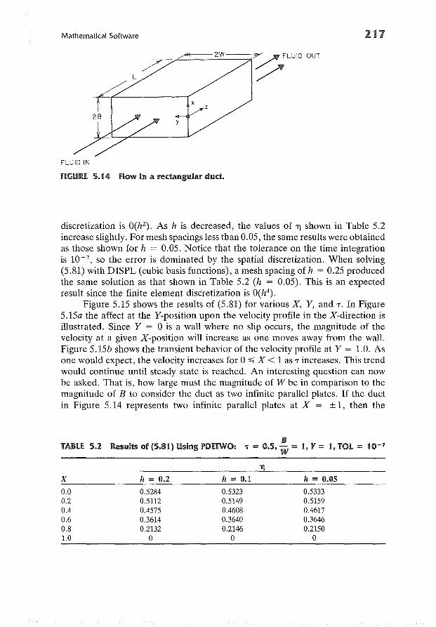
Mathematical Software 217
y
L
~~2W---<?"""'-~LUID OUT
ff------t"xFLUIDIN
fiGURE 5.14 flow In a rectangular duct.
discretization is 0(h2 ). As h is decreased, the values of 'Y] shown in Table 5.2increase slightly. For mesh spacings less than 0.05, the same results were obtainedas those shown for h = 0.05. Notice that the tolerance on the time integrationis 10-7 , so the error is dominated by the spatial discretization. When solving(5.81) with DISPL (cubic basis functions), a mesh spacing of h = 0.25 producedthe same solution as that shown in Table 5.2 (h = 0.05). This is an expectedresult since the finite element discretization is 0(h4 ).
Figure 5.15 shows the results of (5.81) for various X, Y, and 'I". In Figure5.15a the affect at the Y-position upon the velocity profile in the X-direction isillustrated. Since Y = 0 is a wall where no slip occurs, the magnitude of thevelocity at a given X-position will increase as one moves away from the wall.Figure 5.15b shows the transient behavior of the velocity profile at Y = 1.0. Asone would expect, the velocity increases for 0 ~ X < 1 as ,. increases. This trendwould continue until steady state is reached. An interesting question can nowbe asked. That is, how large must the magnitude of W be in comparison to themagnitude of B to consider the duct as two infinite parallel plates. If the ductin Figure 5.14 represents two infinite parallel plates at X = ±1, then the
BTABLE 5.2 Results of (5.81) Using PDETWO: ,. = 0.5, W= 1, Y = 1, TOL = 10- 7
'Y]
X h = 0.2 h = 0.1 h = 0.05
0.0 0.5284 0.5323 0.53330.2 0.5112 0.5149 0.51590.4 0.4575 0.4608 0.46170.6 0.3614 0.3640 0.36460.8 0.2132 0.2146 0.21501.0 0 0 0
218 Partial Differential Equations in Two Space Variables
0.6 ,.--,----,---,.--,----,
1. (b) Y = 1.0, BIW = 1.
LO08
!
0.2 0.4 0.6
X
(b)
(l) 1.00(1) 0.75(3) 0.50(4) 0.15
0.2
0.1
0.5
0.4
TJ 0.3
1.00.6 0.80.4
X
(a)
Results of (5.81).(et) 'T = 0.15, BIW =
Y
(1) 0.15(1) 0.5(3) 1.0
0.2
0.1
0.0 '--_--'--_--'-_---'L.--_--'--_~
o
0.5
0.4
0.3
TJ(2)
0.2
fiGURE 5.15
momentum balance becomes
(5.82)
with
T) = 0 at 'T = 0
T) = 0 at X= 1
aT) = 0 at X = 0axEquation (5.82) possesses an analytic solution that can be used in answering theposed question. Figure 5.16 shows the affect of the ratio B/W on the velocityprofile at various 'T. Notice that at low 'T, a B/W ratio of ~ approximates theanalytical solution of (5.82). At larger 'T this behavior is not observed. To matchthe analytical solution (five significant figures) at all 'T, it was found that thevalue of B/W must be i or less.
Mathematical Software
1.0 ,---,-----,---,----,----,
119
1.0 ,---,-----,---,---,-----,
r =0.5
Y = 1.00.8
0.6
0.4
0.2
0.8
0.6
0.4
02
(3)r= 1.0
Y =1.0
0.0 '--_...L-_--'--__"---_-"-_--'" 0.0 '---_...L-_-----'-__'--_-'-_-'"o 0.2 0.4 0.6 0.8 1.0 0 0.2 0.4 0.6 0.8 1.0
x
FIGURE. 5.16 further results of (5.81).
BIW(1) 1(2) 1/z(3) 1/4 and analytical solution of (5.82)
x
Ellipties
Table 5.3 lists the elliptic PDE software and outlines several features of eachcode. Notice that the NAG library does contain elliptic PDE software, but thisroutine is not very robust. Besides the software shown in Table 5.3, DISPL and2DEPEP contain options to solve elliptic PDEs. Next we consider a practicalproblem involving elliptic PDEs and illustrate the solution and physical implications through the use of DISPL.
The most common geometry of catalyst pellets is the finite cylinder withlength to diameter, LID, ratios from about 0.5 to 4, since they are produced byeither pelleting or by extrusion. The governing transport equations for a finitecylindrical catalyst pellet in which a first-order chemical reaction is occurringare [34]:
where
(Mass)
(Energy)
( )2 []
(Pf 1 af D a2f 'Y- + - - + - - = <p 2f exp - (t - 1)ar 2 r ar L az2 t
( )2 []
a2t 1 at D a2t 2 'Y- + - - - - = -!3<P f exp - (t - 1)ar 2 r ar L az2 t
(5.83)
r = dimensionless radial coordinate, 0 ~ r ~ 1z = dimensionless axial coordinate, 0 ~ z ~ 1
220
f=t =
'Y<P13
Partial Differential Equations in Two Space Variables
dimensionless concentrationdimensionless temperatureArrhenius number (dimensionless)Thiele modulus (dimensionless)Prater number (dimensionless)
with the boundary conditions
af at= 0 at r = 0ar ar
af at0 0- at zaz az
(symmetry)
(symmetry)
f = t = 1 at z = 1 and r 1 (concentration andtemperature specified atthe surface of the pellet)
Using the Prater relationship [35], which is
t = 1 + (1 - f)l3
TABLE 5.3 Elliptic POE Codes
NonlinearEquations Reference
No
No [26]No [27]No [28]No [29]No [30]
No [31]
Code
NAG(D03 chapter)
FISPACKEPDE1ITPACK/REGIONFFf9HLMHLZ/HEL-
MIT/HELSIXIHELSYM
PLTMG
ELIPTI
ELLPACK
Discretization
Finite difference(Laplace's equation
in two dimensions)Finite differenceFinite differenceFinite differenceFinite differenceFinite difference
Finite element; Galerkin with linearbasis functions ontriangular elements
ADI with finite differences; integrateto steady state
Finite difference; finite element (collocation and Galerkin)
Region
Rectangular
RectangularIrregularIrregularIrregularIrregular
Irregular
Irregular
Rectangular
Yes
Yes
[32]
[33]
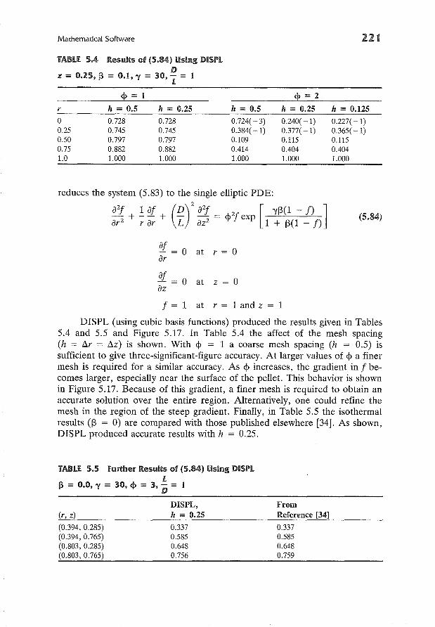
Mathematical Software
TABlE. 5.4 Results of (5.84) Using DlSPLD
Jl = 0.25,13 = 0.1, 'Y = 30, - =L
221
$=1
r h = 0.5 h = 0.25
0 0.728 0.7280.25 0.745 0.7450.50 0.797 0.7970.75 0.882 0.8821.0 1.000 1.000
h = 0.50.724( -3)0.384( -1)0.1090.4141.000
$ = 2
h = 0.25
0.240( -1)0.377( -1)0.1150.4041.000
h = 0.125
0.227( -1)0.365( -1)0.1150.4041.000
reduces the system (5.83) to the single elliptic PDE:
( )2 [ ]
a2f 1 af D a2f 2 'Y13(1 - f)ar 2 + -;. ar + L az2 = <P J exp 1 + 13(1 - f)
af = 0 at r = 0ar
(5.84)
af = 0 at z = 0az
f = 1 at r = 1 and z = 1
DISPL (using cubic basis functions) produced the results given in Tables5.4 and 5.5 and Figure 5.17. In Table 5.4 the affect of the mesh spacing(h = fJ.r = fJ.z) is shown. With $ = 1 a coarse mesh spacing (h = 0.5) issufficient to give three-significant-figure accuracy. At larger values of <p a finermesh is required for a similar accuracy. As <p increases, the gradient in f becomes larger, especially near the surface of the pellet. This behavior is shownin Figure 5.17. Because of this gradient, a finer mesh is required to obtain anaccurate solution over the entire region. Alternatively, one could refine themesh in the region of the steep gradient. Finally, in Table 5.5 the isothermalresults (13 = 0) are compared with those published elsewhere [34]. As shown,DISPL produced accurate results with h = 0.25.
TABlE. 5.5 Further Results of (5.84) Using DISPLL
13 = 0.0, 'Y = 30, $ = 3, D = 1
(r, z)
(0.394, 0.285)(0.394, 0.765)(0.803, 0.285)(0.803, 0.765)
DISPL,h = 0.25
0.3370.5850.6480.756
FromReference [34]
0.3370.5850.6480.759
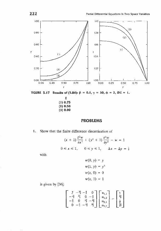
222 Partial Differential E.quations in Two Space Variables
1.000750.50
1.10 F=:::::::J:::::-----,---,---i
1.08
1.06
1.02
1.04
1.00 ,------,-----,---,,-----.1
0.20
0.40
060
080
0.00 ~=::::J=-_--.JL___L__--.J 1.00 ~--~--~-~--~0.00 0.25 0.50 0.75 1.00 0.00 0.25
fiGURE. 5.17 Results of (5.84): p = 0.1, 'Y = 30, <I> = 2, DIL = 1.
!(1) 0.75(2) 0.50(3) 0.00
PROBLEMS
1. Show that the finite difference discretization of
a2 w a2 w(x + 1) - + (y2 + 1) - - w = 1ax 2 ay 2
o :%; x:%; 1, 0 :%; Y :%; 1, Lix = Liy = ~
with
w(O, y) = Y
w(l, y) = y2
w(x,O) = 0
w(x, 1) = 1
is given by [36]:
Problems 223
2.* Consider a rectangular plate with an initial temperature distribution of
w(x, y, 0) = T - To = 0, °~ x ~ 2, °~ y ~ 1
°~ r ~ 1, °~ z ~ 1
3.*
If the edges x = 2, y = 0, and y = 1 are held at T = To and on the edgex = °we impose the following temperature distribution:
() {2tY for °~ Y ~ ~
w 0, Y, t = T - To = 2t(1' _ y), f 1 1or 2: ~ Y ~
solve the heat conduction equation
aw a2w a2w-=-+-at ax2 ay 2
for the temperature distribution in the plate. The analytical solution tothis problem is [22]:
w = ± i i ~ \ (e-O"! + at - 1) sin (WIT) sin (m'Trx) sin (n'TrY)'Trm~ln=ln a 2 2
where
a = 'Tr2 (:2 + n2 )
Calculate the error in the numerical solution at the mesh points.
An axially dispersed isothermal chemical reactor can be described by thefollowing material balance equation:
at = _1 [a2t + ! at] + _1_ a2t + Daz Per ar2 r ar Pea az2 at,
with
1 - t = _1_ at at zPea az
0, at = ° at r = °and r = 1ar
ataz ° a. z = 1
wheret = dimensionless concentration
r = dimensionless radial coordinate
z = dimensionless axial coordinate
Per = radial Peclet number
Pea = axial Peclet number
D a = Damkohler number (first-order reaction rate)
224 Partial Differential Equations in Two Space Variables
The boundary conditions in the axial direction arise from continuity offlux as discussed in Chapter 1 of [34]. Let Da = 0.5 and Per = 10. Solvethe material balance equation using various values of Pea' Compare yourresults to plug flow (Pea -? (0) and discuss the effects of axial dispersion.
4.* Solve Eq. (5.84) with D/L = 1, <p = 1, "y = 30, and let -0.2 ~ 13 ~ 0.2.Comment on the affect of varying 13 [13 < 0 (endothermic), 13 > 0 (exothermic)].
5.* Consider transient flow in a rectangular duct, which can be described by:
a'Y] = a + a2
'Y] + (B) 2 a2
'Y]aT aX2 w ay2
using the same notation as with Eq. (5.81) where a: is a constant. Solvethe above equation with
-(l( Comment
(a) 2(b) 4(c) 1
Eq. (5.81)Twice the pressure gradient as Eq. (5.81)Half the pressure gradient as Eq. (5.81)
How does the pressure gradient affect the time required to reach steadystate?
REFE.RENCE.S
1. Bank, R. E., and D. J. Rose, "Parameter Selection for Newton-LikeMethods Applicable to Nonlinear Partial Differential Equations: SIAM J.Numer. Anal., 17, 806 (1980).
2. Denison, K. S., C. E. Hamrin, and J. C. Diaz, "The Use of PreconditionedConjugate Gradient and Newton-Like Methods for a Two-Dimensional,Nonlinear, Steady-State, Diffusion, Reaction Problem," Comput. Chern.Eng., 6, 189 (1982).
3. Denison, K. S., private communication (1982).
4. Varga, R. S., Matrix Iterative Analysis, Prentice-Hall, Englewood Cliffs,N.J. (1962).
5. Birkhoff, G., M. H. Schultz, and R. S. Varga, "Piecewise Hermite Interpolation in One and Two Variables with Applications to Partial Differential Equations," Numer. Math., 11, 232 (1968).
6. Bramble, J. H., and S. R. Hilbert, "Bounds for a Class of Linear Functionals with Applications to Hermite Interpolation," Numer. Math., 16,362 (1971).
References 225
7. Hilbert, S. R., "A Mollifier Useful for Approximations in Sobolev Spacesand Some Applications to Approximating Solutions of Differential Equations," Math. Comput., 27, 81 (1973).
8. Prenter, P. M., and R. D. Russell, "Orthogonal Collocation for EllipticPartial Differential Equations," SIAM J. Numer. Anal., 13, 923 (1976).
9. Courant, R., "Variational Methods for the Solution of Problems of Equilibrium and Vibrations," Bull. Am. Math. Soc., 49, 1 (1943).
10. Mitchell, A. R., and R. Wait, The Finite Element Method in Partial Differential Equations, Wiley, London (1977).
11. Fairweather, G., Finite Element Galerkin Methods for Differential Equations, Marcel Dekker, New York (1978).
12. Strang, G., and G. J. Fix, An Analysis of the Finite Element Method,Prentice-Hall, Englewood Cliffs, N.J. (1973).
13. Peaceman, D. W., and H. H. Rachford, "The Numerical Solution ofParabolic and Elliptic Differential Equations," J. Soc. Ind. Appl. Math.,3, 28 (1955).
14. Mitchell, A. R., and G. Fairweather, "Improved Forms of the AlternatingDirection Methods of Douglas, Peaceman and Rachford for Solving Parabolic and Elliptic Equations," Numer. Math. 6, 285 (1964).
15. Douglas, J., and J. E. Gunn, "A General Formulation of AlternatingDirection Methods. Part I. Parabolic and Hyperbolic Problems," Numer.Math., 6, 428 (1964).
16. Fairweather, G., and A. R. Mitchell, "A New Computational Procedurefor A.D.I. Methods," SIAM J. Numer. Anal., 163 (1967).
17. Douglas, J. Jr., and T. Dupont, "Alternating Direction Galerkin Methodson Rectangles," in Numerical Solution ofPartial Differential Equations II,B. Hubbard (ed.), Academic, New York (1971).
18. Dendy, J. E. Jr., and G. Fairweather, "Alternating-Direction GalerkinMethods for Parabolic and Hyperbolic Problems on Rectangular Polygons," SIAM J. Numer. Anal., 12, 144 (1975).
19. Schiesser, W., "DSS/2-An Introduction to the Numerical Methods ofLines Integration of Partial Differential Equations," Lehigh Univ., Bethlehem, Pa. (1976).
20. Melgaard, D., and R. Sincovec, "General Software for Two DimensionalNonlinear Partial Differential Equations," ACM TOMS, 7, 106 (1981).
21. Carver, M., et aI., "The FORSIM VI Simulation Package for the Automated Solution of Arbitrarily Defined Partial Differential and/or OrdinaryDifferential Equation Systems, Rep. AECL-5821, Chalk River NuclearLab., Ontario, Canada (1978).
22. Leaf, G. K., M. Minkoff, G. D. Byrne, D. Sorensen, T. Bleakney, andJ. Saltzman, "DISPL: A Software Package for One and Two Spatially
226 Partial Differential Equations in Two Space Variables
Dimensional Kinetics-Diffusion Problems," Rep. ANL-77-12, ArgonneNational Lab., Argonne, Ill. (1977).
23. Sewell, G., "A Finite Element Program with Automatic User-ControlledMesh Grading," in Advances in Computer Methods for Partial DifferentialEquations III, R. Vishnevetsky and R. S. Stepleman (eds.), IMACS (AICA),Rutgers Univ., New Brunswick, N.J. (1979).
24. Hindmarsh, A. c., "GEARB: Solution of Ordinary Differential EquationsHaving Banded Jacobians," Lawrence Livermore Laboratory, Report UCID30059 (1975).
25. Hindmarsh, A. C., "GEAR: Ordinary Differential Equation System Solver," Lawrence Livermore Laboratory Report UCID-3000l (1974).
26. Adams, J., P. Swarztrauber, and N. Sweet, "FISHPAK: Efficient FORTRAN Subprograms for the Solution of Separable Elliptic Partial Differential Equations: Ver. 3, Nat. Center Atmospheric Res., Boulder, Colo.(1978).
27. Hornsby, J., "EPDE1-A Computer Programme for Elliptic Partial Differential Equations (Potential Problems)," Computer Center Program Library Long Write-Up D-300, CERN, Geneva (1977).
28. Kincaid, D., and R. Grimes, "Numerical Studies of Several AdapticeIterative Algorithms," Report 126, Center for Numerical Analysis, Univ.Texas, Austin (1977).
29. Houstics, E. N., and T. S. Papatheodorou, "Algorithm 543. FFT9, FastSolution of Helmholtz-Type Partial Differential Equations," ACM TOMS,5, 490 (1979).
30. Proskurowski, W., "Four FORTRAN Programs for Numerically SolvingHelmholtz's Equation in an Arbitrary Bounded Planar Region," LawrenceBerkeley Laboratory Report 7516 (1978).
31. Bank, R. E., and A. H. Sherman, "PLTMG Users' Guide," Report CNA152, Center for Numerical Analysis, Univ. Texas, Austin (1979).
32. Taylor, J. C., and J. V. Taylor, "ELIPTI-TORMAC: A Code for theSolution of General Nonlinear Elliptic Problems over 2-D Regions ofArbitrary Shape," in Advances in Computer Methods for Partial Differential Equations II, R. Vichnevetsky (ed.), IMACS (AICA), Rutgers Univ.,New Brunswick, N.J. (1977).
33. Rice, J., "ELLPACK: A Research Tool for Elliptic Partial DifferentialEquation Software," in Mathematical Software III, J. Rice (ed.), Academic, New York (1977).
34. Villadsen, J., and M. L. Michelsen, Solution of Differential Equation Modelsby Polynomial Approximation, Prentice-Hall, Englewood Cliffs, N.J. (1978).
35. Prater, C. D., "The Temperature Produced by Heat of Reaction in theInterior of Porous Particles," Chern. Eng. Sci., 8, 284 (1958).
Bibliography 227
36. Ames, W. F., Numerical Methods for Partial Differential Equations, 2nded., Academic, New York (1977).
37. Dixon, A. G., "Solution of Packed-Bed Heat-Exchanger Models by Orthogonal Collocation Using Piecewise Cubic Hermite Functions," MCRTech. Summary Report #2116, University of Wisconsin-Madison (1980).
BIBLIOGRAPHY
An overview offinite difference and finite element methods for partial differential equationsin several space variables has been given in this chapter. For additional or more detailedinformation, see the following texts:
finite Difference
Ames, W. F., Nonlinear Partial Differential Equations in Engineering, Academic, New- York (1965).
Ames, W. F. (ed.), Nonlinear Partial Differential Equations, Academic, New York (1967).
Ames, W. F., Numerical Methods for Partial Differential Equations, 2nd ed., Academic,New York (1977).
Finlayson, B. A., Nonlinear Analysis in Chemical Engineering, McGraw-Hill, New York(1980).
Mitchell, A. R., and D. F. Griffiths, The Finite Difference Method in Partial DifferentialEquations, Wiley, Chichester (1980).
Finite Element
Becker, E. B., G. F. Carey, and J. T. aden, Finite Elements: An Introduction, PrenticeHall, Englewood Cliffs, N.J. (1981).
Fairweather, G., Finite Element Galerkin Methods for Differential Equations, MarcelDekker, New York (1978).
Huebner, K. H., The Finite Element Method for Engineers, Wiley, New York (1975).
Mitchell, A. R., and D. F. Griffiths, The Finite Difference Method in Partial DifferentialEquations, Wiley, Chichester (1980). Chapter 5 discusses the Galerkin method.
Mitchell, A. R., and R. Wait, The Finite Element Method in Partial Differential Equations,Wiley, New York (1977).
Strang, G., and G. J. Fix, An Analysis of the Finite Element Method, Prentice-Hall,Englewood Cliffs, N.J. (1973).
Zienkiewicz, O. C., The Finite Element Method in Engineering Science, McGraw-Hill,New York (1971).
APPENDIX
Computer ArithmeticError Control
In mathematical computations on a computer, errors are introduced into thesolutions. These errors are brought into a calculation in three ways:
1. Error is present at the outset in the original data-inherent error
2. Error results from replacing an infinite process by a finite one-truncationerror, i.e., representing a function by the first few terms of a Taylor seriesexpansion
3. Error arises as a result of the finite precision of the numbers that can berepresented in a computer-round-off error.
Each of these errors is unavoidable in a calculation, and hence the problem isnot to prevent their occurrence, but rather to control their magnitude. Thecontrol of inherent error is not within the scope of this text, and the truncationerrors pertaining to specific methods are discussed in the appropriate chapters.This section outlines computer arithmetic and how it influences round-off errors.
COMPUTER NUMBER SYSTEM
The mathematician or engineer, in seeking a solution to a problem, assumesthat all calculations will be performed within the system of real numbers, !7{.
In !7{, the interval between any two real numbers contains infinitely many realnumbers. !7{ does not exist in a computer because there are only a finite amount
229
230 Computer Arithmetic and Error Control
of real numbers within a computer's number system. This is a source of roundoff error. In computer memory, each number is stored in a location that consistsof a sign (±) plus a fixed number of digits. A discussion of how these digitsrepresent numbers is presented next.
NORMALIZED fLOATING-POINT NUMBER SYSTEM
A floating-point number system is characterized by four parameters:
~ = number base
t = precision
L, U = exponent range.
One can denote such a system by
F(~, t, L, U)
Each floating-point number, x#.o, in F is represented in the following way:
x = + (d1 + d2 + + dt) x Qe (A.I)
- ~ ~2 ..• W tJ
where
The fact that d1 #. 0 means that the floating-point number system is normalized.
ROUND-Off ERRORS
Next, consider the differences between computations in Fversus 9l, i.e., roundoff errors. The source of the differences lies in the fact that F is not closed underthe arithmetric operations of addition and multiplication (likewise, subtractionand division); the sum or the product of two numbers in F may not necessarilybe an element of F. Hence, to stay in F, the computer replaces the "true" resultof an operation by an element of F, and this process produces some error.Several cases can occur [A.4]:
1. The exponent e of the result can lie outside the range L ~ e ~ U,(a) If e > U, overflow; for example, in F(2, 3, -1, 2) (A.2)
(0.100 x 22) x (0.110 X 22) = 0.110 X 2d
2 x 3 6
Round-Off E.rrors 231
(b) If e < L, underflow; for example, in F(2, 3, -1, 2)(0.100 x 2°) x (0.110 x 2- 1
) = 0.110 X 22.133- X - -2 8 16
(A.3)
2. The fractional part has more than t digits; for example, considerF(2, 3, -1,2)(0.110 x 2°) + (0.111 x 2°) = 0.1101 X 21
3 7 13- + - -488
(notice that four digits are required to represent the fractional part). Similarly,(0.111 x 2°) x (0.110 x 2°) = 0.10101 x 2°
7 3 21- x - -8 4 32
(while this situation does not arise frequently in addition, it almost invariablydoes with multiplication).
To define a result that can be represented in the machine, the computer selectsa nearby element of F. This can be done in two ways: rounding and chopping.Suppose the "true" result of an operation is
(A.4)
then,
x 21 : rounding,
~0.110
X 21
------ 0.111
0.1101
1. Chopping: digits beyond (dt)/(W) are dropped.
2. Rounding:
(d1 d2 dt + 1 + ~ 13) x Qe13 + 132 + ... + W+ 1 I-'
then chop.
For example, if one considers F(2, 3, -1, 2), the number
x 21 : chopping
while for
0.10101 x
.----.. 0.101
2°
--------.. 0.101
x 2°: chopping
x 2°: rounding.
232 Computer Arithmetic and Error Control
Both methods are commonly used on present-day computers. No matter themethod, there is some round-off error introduced by the process. If f(x) represents the machine representation of x, then
Ix -xf(X)I,a(x) = relative round-off error = X =1= 0
(A.S)
It can be shown that [A.1]
{f3 1- t • chopping
a(x) ~ EPS = -21 Q.2~t.. d'fJ roun mg
As an example, suppose X = 12.467 with F(lO, 4, - 50, 50) and chopping, thenf(x) = 0.1246 X 10² and
( )= 112.467 - 0.1246 x 1021
a X 12.467
or
a(x) = 0.00056 < EPS = 10-3
For the same system with rounding, f(x) = 0.1247 X 10⁻² and
a(x) = 0.00024 < EPS = ! X 10-3
One can see that the parameter EPS plays an important role in computationwith a floating-point number system. EPS is the machine epsilon and is definedto be the smallest positive machine number such that
f(1 + EPS) > 1,
For example, for F(lO, 4, - 50, 50) with chopping
EPS = 10-3 since f(1 + 0.001) = 0.1001 x 101 > 1
and for rounding
EPS = 0.0005 since f(1 + 0.0005) = 0.1001 x 101 > 1
The machine epsilon is an indicator of the attainable accuracy in a floating-pointnumber system and can be used to determine the maximum achievable accuracyof computation.
Take, as a specific example, an IBM 3032 and find EPS. Considering onlyfloating-point number systems, the IBM 3032 uses either of two base 16 systems:
1. Fs (16, 6, - 64, 63): single precision
2. Fv(16, 14, - 64, 63): extended precision
For chopping (EPS = f31-t):
EPS (single) = 9.54 x 10⁻⁷
EPS (extended) = 2.22 x 10⁻¹⁶
Round-Off Errors 233
If one executes the following algorithm (from Forsythe, Malcolm, and Moler[A.1]):
OOUBLE PRECISION EPS, EPS1EPS = 1.00
10 EPS = 0.500*EPSEPS1 = EPS + 1.00IF (EPS1. GT. 1.00) GO TO 10WRITE (6,20) EPS
20 FORMAT (5X, 'THE MACHINE EPSILON = ',017.10)STOPENO
the result is:
THE MACHINE EPSILON = 0.1110223025 0-15
This method of finding EPS can differ from the "true" EPS by at most a fractionof 2 (EPS is continually halved in statement number 10). Notice that the calculated value of EPS is half of the value predicted by EPS = 13 1 - t
, as one wouldexpect. In the course of carrying out a computer calculation of practical magnitude, a very large number of arithmetic operations are performed, and theerrors can propagate. It is, therefore, wise to use the number system with thegreatest precision.
Another computational problem involving the inability of the computer torepresent numbers of 9( in F is shown below. Take for instance the number0.1, which is used frequently in the partition of intervals, and consider whetherten steps of length 0.1 are the same as one step of length 1.0. If one executesthe following algorithm on an IBM 3032:
OOUBLE PRECISION XX = 0.00N = 000 10 I = 1,10X = X + 0.100
10 CONTINUEIF (X.EQ.1.00) N = 1WRITE(6,20) N,X
20 FORMAT (1 OX,' THE VALUE OF N = ',11,/,10X,*' THE VALUE OF X = ',017.10)
STOPENO
the result is:
THE VALUE OF N = 0THE VALUE OF X = 0.1000000000001.
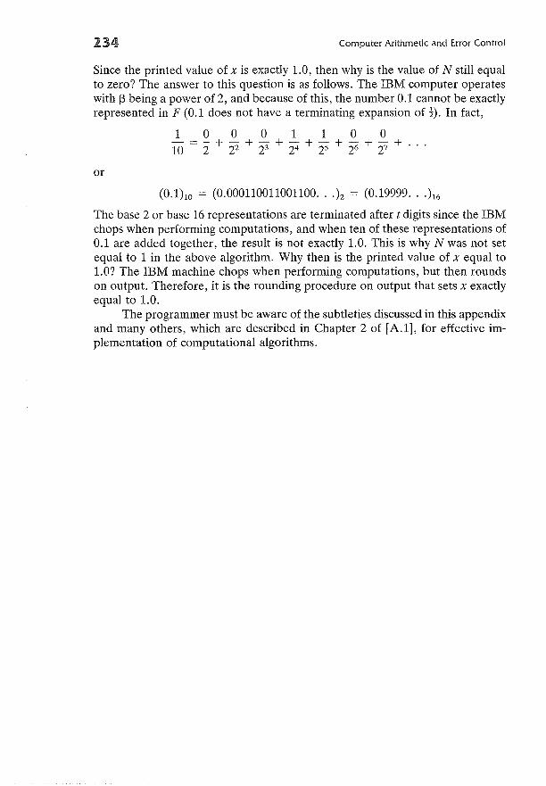
234 Computer Arithmetic and Error Control
Since the printed value of x is exactly 1.0, then why is the value of N still equalto zero? The answer to this question is as follows. The IBM computer operateswith 13 being a power of 2, and because of this, the number 0.1 cannot be exactlyrepresented in F (0.1 does not have a terminating expansion of ~). In fact,
1000110010 = 2: + 22 + 23 + 24 + 25 + 26 + 27 + . . .
or
(0.1)10 = (0.000110011001100...)z = (0.19999.. ')16
The base 2 or base 16 representations are terminated after t digits since the IBMchops when performing computations, and when ten of these representations of0.1 are added together, the result is not exactly 1.0. This is why N was not setequal to 1 in the above algorithm. Why then is the printed value of x equal to1.0? The IBM machine chops when performing computations, but then roundson output. Therefore, it is the rounding procedure on output that sets x exactlyequal to 1.0.
The programmer must be aware of the subtleties discussed in this appendixand many others, which are described in Chapter 2 of [A.1], for effective implementation of computational algorithms.
APPENDIX
Newton's
(B.t)
Systems of nonlinear algebraic equations arise in the discretization of differentialequations. In this appendix, we illustrate a technique for solving systems ofnonlinear algebraic equations. More detailed discussions of this topic can befound in [A.1-A.4].
Consider the set of nonlinear algebraic equations
fl(Yv Yz, ... ,Yn) = 0
f2(YV Yz,·· ·,Yn) = 0
which can be written as
i = 1,2, ... , n,
or
fey) = 0
We wish to find that set {YAi = 1, ... , n} that satisfies (B.1).Although there are many ways to solve Eq. (B.1), the most common
method of practical use is Newton's method (or variants of it). In the case of asingle equation, the Newton method consists in linearizing the given equationfey) = 0 by approximatingf(y) by
f(yO) + f' (yO)(y - yO) (B.2)
235
236 Newton's Method
where yO is believed to be close to the actual solution, and solving the linearizedequation
(B.3)
The value yl = yO + Lly is then accepted as a better approximation, and theprocess is continued if necessary.
Now consider the system (B.l). If the ith equation is linearized, then
fi(Y~' y~, ... , y~) + ±[aaft
! (yJ+l - yn] = 0 (B.4)J~ 1 YJ k
where k ;;;: O. The Jacobian is defined as
II<. = a/; IIJ aYj k
and (B.4) can be written in matrix form as
Jk Lly = - f(yk)
where
The procedure is
1. Choose yO
2. Calculate Lly from (B.6)
3. Set yk+l = yk + Lly
4. Iterate on (2) and (3) until
IILlyllx < TOL
where
Ilxllx = max Xi
TOL = arbitrary
(B.S)
(B.6)
The convergence of the Newton method is proven in [A.2] under certain conditions, and it is shown that the method converges quadratically, i.e.,
(B.7)
where
f(g*) = 0
and
m = a constant
APPENDIX
Gaussian Elimination
From the main body of this text one can see that all the methods for solvingdifferential equations can yield large sets of equations that can be formulatedinto a matrix problem. Normally, these equations give rise to a matrix havinga special property in that a great many of its elements are zero. Such matricesare called sparse. Typically, there is a pattern of zero and nonzero elements,and special matrix methods have been developed to take these patterns intoconsideration. In this appendix we begin by discussing a method for solving ageneral linear system to equations and then proceed by outlining a method forthe tridiagonal matrix.
DENSE MATRIX
The standard method of solving a linear system of algebraic equations is to doa lower-upper (LU) decomposition on the matrix, or Gaussian elimination.Consider a dense (all elements are nonzero), nonsingular (all rows or columnsare independent) n x n matrix A such that
Ax = r
231
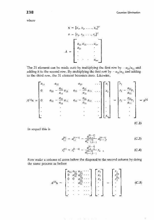
238
where
A
x = [Xl> X2' ... , Xn]T
Gaussian Elimination
The 21 element can be made zero by multiplying the first row by - a 2l /a ll andadding it to the second row. By multiplying the first row by - a3l/a ll and addingto the third row, the 31 element becomes zero. Likewise,
all a12 al3 Xl r l
0a 2l a 2l a2l
a 22 - -al2 a 23 - -al3 X2 r2 -rlall all all
A[l]X 0a3l a3l a3l
r[l]a32 - -al2 a33 - -al3 r3 - -rlall all all
(C.2)
In sequel this is
a[k-l]'-l
r[k] = r[k-l] _I I
a[k-l]i.k-l [k-l]
[k-l] a k - l •pak-l,k-l
a[k-l]i.lc-l
[k-l] r k - lalc-l,lc-l
(C.3)
(C.4)
Now make a column of zeros below the diagonal in the second column by doingthe same process as before
all a l2 a 13 .• Xl r l0 a[2] a[2] .. X2
r[2]22 23 2
0 0 a[2] . X 3r[2]
33 3A[2]x a[2] • (C.S)43
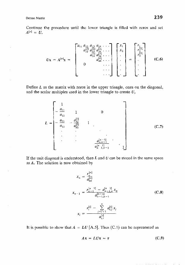
Dense Matrix 139
Continue the procedure until the lower triangle is filled with zeros and setA[n] = V.
Vx = A[n]x
o(C.6)
Define L as the matrix with zeros in the upper triangle, ones on the diagonal,and the scalar multiples used in the lower triangle to create V,
1a 21
1 0all
a 31a[2]
L 32 1all
- a[2](C.7)22
a[n-l]n,n -1
a[n-l]1n-l.n-l
If the unit diagonal is understood, then L and V can be stored in the same spaceas A. The solution is now obtained by
r[n-l] _ a[n-l] xn-l n-l.n n
a[n-l]n-l,n 1
(C.S)
Xi
n
~j=i+l
ali] x.l,J J
It is possible to show that A = LV [A.5]. Thus (C.l) can be represented as
Ax = LVx = r (C.9)
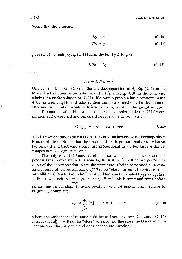
240
Notice that the sequence
Ly = r
Ux = y
gives (C.9) by multiplying (Cll) from the left by L to give
LUx = Ly
or
Gaussian Elimination
(C.IO)
(c.n)
(C.12)
Ax = LUx = r
One can think of Eq. (C.3) as the LV decomposition of A, Eq. (C.4) as theforward substitution or the solution of (C.10), and Eq. (C.S) as the backwardelimination or the solution of (Cll). If a certain problem has a constant matrixA but different right-hand sides r, then the matrix need only be decomposedonce and the iteration would only involve the forward and backward sweeps.
The number of multiplications and divisions needed to do one LV decomposition and m-forward and backward sweeps for a dense matrix is
OPG.E. = ~ n3- ~ n + mn2 (C.B)
This is fewer operations than it takes to calculate an inverse, so the decompositionis more efficient. Notice that the decomposition is proportional to n3
, whereasthe forward and backward sweeps are proportional to n2
• For large n the decomposition is a significant cost.
The only way that Gaussian elimination can become unstable and theprocess break down when A is nonsingular is if ali-I] = 0 before performingstep i of the decomposition. Since the procedure is being performed on a computer, round-off errors can cause ali-I] to be "close" to zero, likewise, causinginstabilities. Often this round-off error problem can be avoided by pivoting; thatis, find row s such that max \aJi- 11 \ = al~-l] and switch row s and row i before
i~I~n
performing the ith step. To avoid pivoting, we must impose that matrix A bediagonally dominant:
n
laul ~ 2: laiA,j~1
joFi
i = 1, ... , n, (C.14)
where the strict inequality must hold for at least one row. Condition (C.14)insures that a!;-l] will not be "close" to zero, and therefore the Gaussian elimination procedure is stable and does not require pivoting.
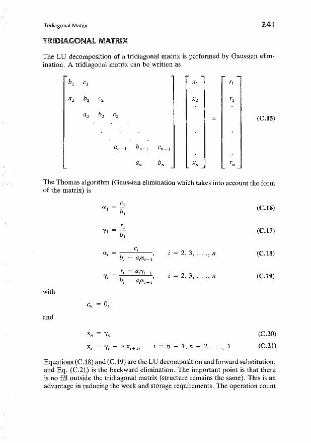
Tridiagonal Matrix
TRIDIAGONAL MATRIX
241
The LV decomposition of a tridiagonal matrix is performed by Gaussian elimination. A tridiagonal matrix can be written as
Xz
(C.IS)
The Thomas algorithm (Gaussian elimination which takes into account the formof the matrix) is
with
and
r i - ai'Yi-l'Yi = ,
hi - aiOl.i - 1
i = 2,3, ... , n
i = 2,3, ... , n
(C.16)
(C.17)
(C.lS)
(C.19)
i = n - 1, n - 2, ... , 1
(C.20)
(C.21)
Equations (C.18) and (C.19) are the LV decomposition and forward substitution,and Eq. (C.21) is the backward elimination. The important point is that thereis no fill outside the tridiagonal matrix (structure remains the same). This is anadvantage in reducing the work and storage requirements. The operation count
242
to solve m such systems of size n is
Gaussian Elimination
OPTD = 2(n - 1) + m(3n - 2),
which is a significant savings over mn3 of (C.13). Since this algorithm is a specialform of Gaussian elimination without pivoting, the procedure is stable only whenthe matrix possesses diagonal dominance.
APPENDIX
In finite element methods the manner in which the approximate numerical solution of a differential equation is represented affects the entire solution process.Specifically, we would like to choose an approximating space of functions thatis easy to work with and is capable of approximating the solution accurately.Such spaces exist, and bases for these spaces can be constructed by using Bsplines [A.6]. The authoritative text on this subject is by deBoor [A.6].
Before defining the B-splines, one must first understand the meaning of adivided difference and a truncated power function. The first-order divided difference of a function g(X) , Xi ~ X ~ Xi+h is
(D.I)
while the higher-order divided difference (dd) formulas are given by recursionformulas: the rth-order dd of g(x) on the points Xi' Xi + l' ... , Xi + r is
where
[ ]g[Xi+h"" x i + r] - g[xi, ... , xi+r-d
g Xi' Xi+ h ... ,Xi+r =Xi + r - Xi
(D.2)
g[Xi, ... , xi+r-dg[Xi+1' ... , Xi+r-d - g[Xi, ..• , Xi+r-Z]
Xi + r - 1 - Xi
243
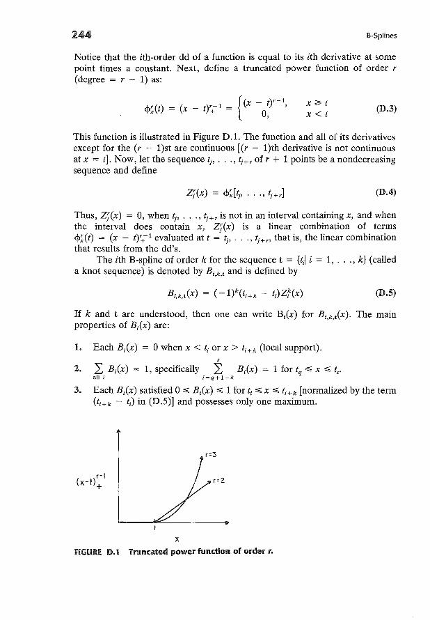
244 B-Splines
Notice that the ith-order dd of a function is equal to its ith derivative at somepoint times a constant. Next, define a truncated power function of order r(degree = r - 1) as:
x~t
x<t(D.3)
This function is illustrated in Figure D.1. The function and all of its derivativesexcept for the (r - l)st are continuous [(r - l)th derivative is not continuousat x = t]. Now, let the sequence tj , ••• , tj +r of r + 1 points be a nondecreasingsequence and define
(D.4)
Thus, Zj(x) = 0, when tj , ••• , tj +r is not in an interval containing x, and whenthe interval does contain x, Zj(x) is a linear combination of terms<p~(t) = (x - t)':t-- 1 evaluated at t = tj , ••• , tj +n that is, the linear combinationthat results from the dd's.
The ith B-spline of order k for the sequence t = {til i = 1, ... , k} (calleda knot sequence) is denoted by Bi,k,t and is defined by
(D.S)
If k and t are understood, then one can write B/x) for Bi,k,t(X). The mainproperties of Bi(x) are:
1. Each B/x) = °when x < ti or x> ti+k (local support).s
2. ~ B/x) = 1, specifically ~ Bi(x) = 1 for tq ~ x ~ ts •all i i=q+l-k
3. Each B/x) satisfied°~ Bi(x) ~ 1 for ti ~ x ~ ti+k [normalized by the term(ti+k - ti) in (D.S)] and possesses only one maximum.
fiGURE D.l
xTruncated power function of order 1'.
B-Splines 245
Consider the approximating space .0'1'(1T) (described in Chapter 3) andwhether the B-splines can serve as a basis for this space. Given the partition 1T,
a = Xl < X2 < ... < Xe+l = b, (D.6)
(D.7)
and the nonnegative integer sequence 11 = {Vj/j = 2, ... , e}, which denotesthe continuity at the breakpoints Xi> then the dimension of .0'1'(1T) is given by
eN = dim ~(1T) = 2": (k - Vj)
j=l
with VI = O. If t = {tili = 1, ... , N + k} such that
tl :s;; t2 :s;; ... :s;; tk :s;; Xl (makes the first B-spline one at Xl)
(makes the last B-spline one at Xe+l)
and if for i = 2, ... , e, the number Xi occurs exactly k - Vi times in the set t,then the sequence B;(x), i = 1, ... , N is a basis for ~(1T) [A.6]. Thereforea function f(x) can be represented in ~(1T) by
N
f(x) = 2": cxiB;(X)i=l
(D.9)
The B-splines have many computational features that are described in[A.6]. For example, they are easy to evaluate. To evaluate a B-spline at a pointX, tj :s;; X :s;; tj+l , the following algorithm can be used [A.7] [let Bi,k,t(X) bedenoted by Bi,k and Z7(x) by Zi,k]:
Bi,l = 1
DO 20 e = 1, . . ., k - 1
Bi-e,e+l = 0
DO 10 j = 1, . . ., eZi+j-e,e = Bi+j-e,ef(ti+j - ti+l - e)
Bi+j-e-l,e+l = Bi+j-e-l,e+l + (ti+j - X)Zi+j-e,e
Bi+j-e,e+l = (x - ti+j-e)Zi+j-e,e
10 CONTINUE
20 CONTINUE
Thus B-splines of lower order are used to evaluate B-splines of higher order. Acomplete set of algorithms for computing with B-splines is given by deBoor[A.6].
A B-spline Bi,k,t(X) has support over [ti, ' .. , ti+k]' If each point Xi appearsonly once in t, that is, Vi = k - 1, then the support is k subintervals, and theB-spline has continuity of the k - 2 derivative and all lower-order derivatives.
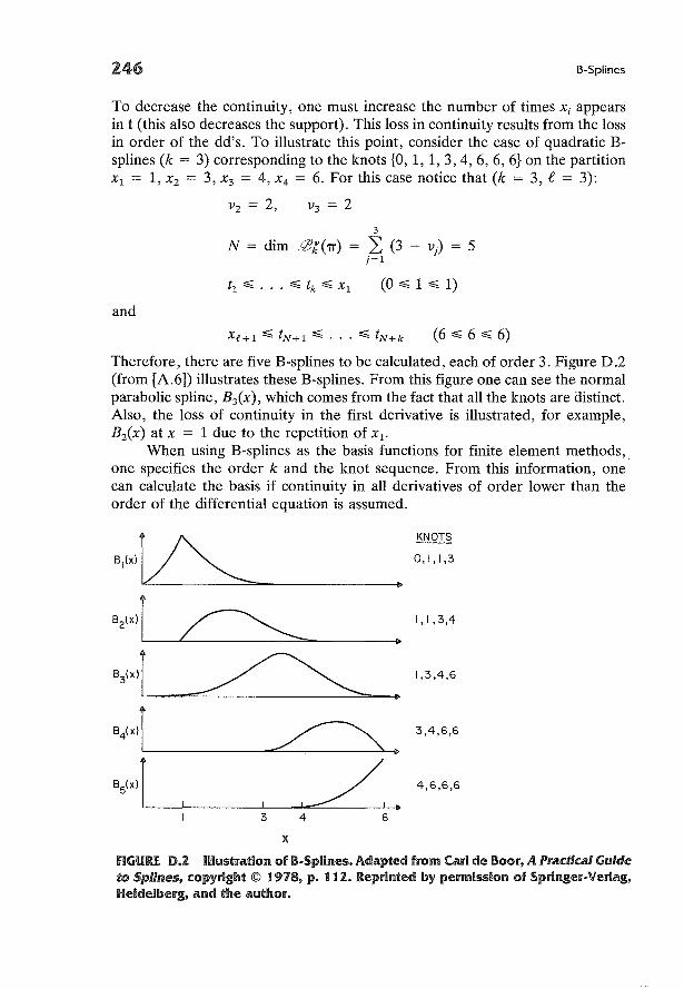
246 B-Splines
To decrease the continuity, one must increase the number of times Xi appearsin t (this also decreases the support). This loss in continuity results from the lossin order of the dd's. To illustrate this point, consider the case of quadratic Bsplines (k = 3) corresponding to the knots {O, 1, 1,3,4,6,6, 6} on the partitionXl = 1, Xz = 3, X3 = 4, X4 = 6. For this case notice that (k = 3, e = 3):
Vz = 2,
3
N = dim .fB{('TT) = L (3 - v) = 5J=l
(0 ~ 1 ~ 1)
and
(6 ~ 6 ~ 6)
Therefore, there are five B-splines to be calculated, each of order 3. Figure D.2(from [A.6]) illustrates these B-splines. From this figure one can see the normalparabolic spline, B3(x), which comes from the fact that all the knots are distinct.Also, the loss of continuity in the first derivative is illustrated, for example,Bz(x) at X = 1 due to the repetition of Xl'
When using B-splines as the basis functions for finite element methods,one specifies the order k and the knot sequence. From this information, onecan calculate the basis if continuity in all derivatives of order lower than theorder of the differential equation is assumed.
B""~B21"l_£--~__-----=",,---- ~
B,"'l-----===-------=----+B4(X)1L- ~"""_______----"'_~
BS'" 1--'-_--'----"-,L-=:.----,---+!
KNOTS
0,1,1,3
1,1,3,4
1,3,4,6
3,4,6,6
4,6,6,6
3 4 6
xFIGURE D.2 Illustration of B.Splines. Adapted from Carl de Boor, A Practical Guideto Splines, copyright © t 978, p. t t 2. Reprinted by permission of Springer.Verlag,Heidelberg, and the author.
APPENDIX
Iterative Matrix
Consider the solution of the linear algebraic system
Ax = b (E.1)
where A is a given real N x N matrix, b is a given N component vector, and xis the unknown vector to be determined. In this appendix we are concernedwith systems in which N is large and A is sparse. Linear systems of this typearise from the numerical solution of partial differential equations.
After discretizing a partial differential equation by either finite differenceor finite element techniques, one is faced with the task of solving a large sparsesystem of linear equations of form (E.1). Two general procedures used to solvesystems of this nature are direct and iterative methods. Direct methods are thosethat, in the absence of round-off errors, yield the exact solution in a finite numberof arithmetic operations. An example of a direct method is Gaussian elimination.Iterative methods are those that start with an initial guess for the solution andthat, by applying a suitably chosen algorithm, lead to better approximations. Ingeneral, iterative methods require less storage and fewer arithmetic operationsthan direct methods for large sparse systems (for a comparison of direct anditerative methods, see [A.8]).
An iterative method for the solution of linear systems is obtained by splitting the matrix A into two parts, say
A=S-T
To solve (E.1) define a sequence of vectors xe by
(E.2)
e = 0,1, . (E.3)
147
248 Iterative Matrix Methods
where XO is specified. If the sequence of vectors converges, then the limit willbe a solution of (E.1).
There are three common splittings of A. The first is known as the pointJacobi method and is
S=D
T=D-A(E.4)
where the matrix D is the diagonal matrix whose main diagonal is that of A. Incomponent form the point Jacobi method is
l~i~N, e~o (E.5)
An obvious necessary condition for (E.5) to work is au 1= O. If A is diagonallydominant, then the point Jacobi method converges [A.3]. Examination of (E.5)shows that one must save all the components of xe while computing xe+ 1
• TheGauss-Seidel method does not possess this storage requirement. The matrixsplitting equations for the Gauss-Seidel method are
S=D+L
T = -U
(E.6)
where D is as before, and U and L are strictly upper and lower triangular matrices,respectively. In component form this method is
i-I a.. Nabxe+1 = - 2: 3. Xf+l - 2: -!!. xf + -.!.,
I j=1 aii J j=i+l aii aii
1 ~ i ~ N, e~ o. (E.7)
As with the point Jacobi method, A must be diagonally dominant for the GaussSeidel method to converge [A.3]. Also, in most practical problems the GaussSeidel method converges faster than the point Jacobi method. The third commonmethod is closely related to the Gauss-Seidel method. Let the vector xe+ 1 bedefined by
i-I a Nab.2: -!!. xf + 1 - 2: -!!. xJ + -'-,j~1 au j~i+l au au
1 ~ i ~ N, e~ 0 (E.8)
from which xe+ 1 is obtained as
Xf+l = xf + W(if+l - xi)or
Xf+l = (1 - w)xf + Wif+l (E.9)
The constant w, 1 ~ w ~ 2, is called the relaxation parameter, and is chosen toaccelerate the convergence. Equations (E.8) and (E.9) can be combined to give
b· }+ -'- - xfaii
1 ~ i ~ N, e ~ 0 (E.I0)
Appendix References 249
Notice that if w = 1, the method is the Gauss-Seidel method. Equation (E.lO)can be written in the split matrix notation as
1S = - [D + wL]
w
1T = - [(1 - w)D - wU]
w
(E.ll)
where D, L, and U are as previously defined. This method is called successiveover relaxation (SOR). In the practical use of SOR, finding the optimal w is ofmajor importance. Adaptive procedures have been developed for the automaticdetermination of w as the iterative procedure is being carried out (see, forexample [A9]).
Computer packages are available for the solution of large, sparse linearsystems of algebraic equations. One package, ITPACK [AlO], contains research-oriented programs that implement iterative methods.
APPENDIX REFERENCES
A.I. Forsythe, G. E., M. A Malcolm, and C. B. Moler, Computer Methodsfor Mathematical Computations, Prentice-Hall, Englewood Cliffs, N.J.(1977).
A.2. Keller, H. B., Numerical Solution of Two Point Boundary Value Problems, SIAM, Philadelphia (1976).
A.3. Finlayson, B. A., Nonlinear Analysis in Chemical Engineering, McGrawHill, New York (1980).
A.4. Johnston, R. L., Numerical Methods-A Software Approach, Wiley,New York (1982).
A.5. Forsythe, G., and G. B. Moler, Computer Solution of Linear AlgebraicSystems, Prentice-Hall, Englewood Cliffs, N.J. (1967).
A.6. deBoor, C., Practical Guide to Splines, Springer-Verlag, New York(1978).
A.7. Russell, R. D., Numerical Solution of Boundary Value Problems, Lecture Notes, Universidad Central de Venezuela, Publication 79-06, Caracas (1979).
A.S. Eisenstat, S., A. George, R. Grimes, D. Kincaid, and A. Sherman,"Some Comparisons of Software Packages for Large Sparse Linear Systems," in Advances in Computer Methods for Partial Differential Equations III, R. Vichneveshy and R. S. Stepleman (eds.), IMACS (AICA),Rutgers University, New Brunswick, N.J. (1979).
250, Iterative Matrix Methods
A.9. Kincaid, D. R., "On Complex Second-Degree Iterative Methods," SIAMJ. Numer. Anal., 2, 211 (1974).
A.10. Grimes, R. G., D. R. Kincaid, W. I. MacGregor, and D. M. Young,"ITPACK Report: Adaptive Iterative Algorithms Using Symmetric SparseStorage," Report No. CNA-139, Center for Numerical Analysis, Univ.of Texas, Austin, Tex. (1978).
Adams, J., 226Addison, C.A., 51Alexander, R., 29, 50Allen, R.H., 28, 50Ames, W.F., 174, 175,227Aris, R., 126Ascher, D., 126Ariz, A.Z., 95
Bank,R.E., 184, 185,224,226Becker,E.B., 126, 175,227Bickart, T.A., 51Bird, R.B., 94, 126, 137Birkhoff, G., 194,224Bleakney, T., 174,225Bramble, I.H., 194,224Brown, D.R., 94Brown, H.G., 51Bui, T.D., 29, 50Bui, T.R., 29, 50Bulirsch, R., 94Burka, M.K., 29, 50Burrage, K., 51Butcher, J .C., 51Butt, I.B., 5, 49,173Byrne, G.D., 51,174,225
Caillaud, I.B., 28, 33,42,43,44,50
Calahan, D., 28, 50Carberry, J.J., 93Carey, G.F., 126, 147, 173, 175,227Carver, M., 174,225Childs, B., 95Chipman, F.H., 51Christiansen, J., 126Conte, S.D., 49Courant, R., 205, 225Craigie, I.A. 1., 51Crowther, C.R., 51
Daniel, J.W., 95Davenport, S.M., 39, 51Davis, M.E., 90, 94,126,144,146,173deBoor, C., 49, 120, 125, 126,247Dendy, J.E., Jr., 214, 225Denison, K.S., 224Denman, E., 95Deuflhard, P., 93, 94Dew, P.M., 173Diaz, J .C., 118, 126,224Dixon, A.D., 227Douglas, J., Jr., 142, 172,214,225DuPont, T., 214, 225
Eisenstat, S., 247England, R., 94
251
252
Enright, W.H., 39, 51
Fairweather, G., 90, 94,125,126,146,173,175,214,225,227
Fellen, B.M., 39, 51Finlayson, B.A., 42, 52,175,227,249Fix, G.J., 126, 175,225,227Forsythe, G.E., 50, 52,175,233,249Fox, L., 86, 93,95, 126Fox, P.A., 174Froment, G.F., 174
Gaffney, P.W., 51Gear, C.W., 36, 49, 52George, A., 247Gladwell, 1., 51, 95Gordon, M.K., 49, 52,173Griffiths, D.F., 172, 175,227Grimes, R.G., 226, 247, 250Gunn, J.E., 214, 225
Hall, A.D., 52, 126, 174Hamrin, C.E., 224Hicks, J.S., 94Hilbert, S.R., 194,224,225Hindmarsh, A.C., 51, 173,226Hornsby, J., 226Houstics, E.N., 226Hueber, K.H., 227Hull, T.E., 39, 51Hwang, M., 42, 52Hyman, J.M., 174
Isaacson, E., 95,175
Jackson, K.R., 51Johnston, R.L., 37, 49, 52, 247Jones,B.F., 142, 172
Keast, P., 126Kehoe, J.P.G., 5,49,173Keller, H.B., 56, 93, 95,175,249Kincaid, D., 226, 249, 250Kong, A.K., 51,147,173Krogh, F.T., 37, 50
Lambert, J.D., 50, 52Lapidus, L., 42,52Leaf,G.K., 174,225Lees, M., 142, 173Lentini, M., 89, 94Lightfoot, E.N., 94,126,137Lindberg, B., 39, 51Liskovets, O.A., 172
Author Index
MacGregor, W.1., 250Madsen, M.K., 174Malcolm, M.A., 50, 52, 233, 249Melgaard, D., 225Michelsen, M.L., 33, 37, 42, 50, 52,174,226Minkoff, M., 174,225Mitchell, A.R., 172, 175,214,225,227Moler, C.B., 50, 52, 233, 249Murray, J.D., 81, 93
Nelson, P., 95Norsett, S.P., 29, 50
Oden,J.T., 126, 175,227
Padmanabhan, L.,28,33,42,43,44, 50Papatheodorou, T.S., 226Peaceman, D.W., 214, 225Pereyra, V., 86, 89, 93, 94Pice!, Z., 51Poots, J., 126Prater, C.D., 226Prenter, P.M., 195,225Price, T.H., 5, 49Proskurowski, W., 226
Rachford, H.H., 214, 225Rice, J., 226Robertson, A.H., 41, 52Rose, D.J., 184, 185,224Rosenbrock, H.H., 50Russell, R.D., 95, 126, 195,225,247
Salariya, A.K., 94Saltzman, J., 174,225Sayers, D.K., 95Schiesser, W., 174,225Schryer, N.L., 126, 174Schultz, M.H., 194,224Scott, M.R., 93, 94, 95Sedgwick, A.E., 39, 51Seinfeld, J.H., 42, 52Sepehrnoori, K., 147, 173Sewell, G., 21, 226Shampine, L.F., 39, 49, 50, 51, 52,173Sherman, A.H., 226, 249Sincovec, R.F., 174,225Skeel, R.D., 51,147,173Sorensen, D., 174,225Stewart, W.E., 94, 126, 137Strang, G., 126, 175,225,227Swartz, B., 126Swarztrauber, P., 226Sweet, N., 226

Author Index
Taylor, J.C., 226Taylor, J.V., 226Tendler, J.M., 51
Varah, J.M., 118Varga, R.S., 93, 95, 126, 185, 191, 194,
224Verwer, J.G., 51,173Villadsen, J., 42, 50, 52,174,226
Wait, R., 175,225,227
Walsh, LE., 173Watson, W.R., 175Watts, H.A., 39, 50, 51, 52, 93, 94Weiss, R., 126Weisz, P.B., 94Wilkes, J.O., 137, 172
Yamanis, J., 144, 146, 173Young, D.M., 250
Zienkiewicz, O.C., 227
253
Adams-Bashforth predictor-corrector method,24,25,27,39,40
Adams-Moulton predictor-corrector method, 26,33,39,40
Adiabatic, 34Alternating direction implicit methods (ADI),
212-214Annular bed reactor, 144-146, 187-190Approximating space, 97-106, 109, 194,200,
201,243,245Autonomous, 28, 34Axial dispersion, 187-190
Backward difference approximation, 68, 132,133, 134, 139-142
Backward elimination, 240, 241Basis functions, 97-103, 154, 158, 159, 194,200,
201,205,207,208,210,211Batch still, 21-24Bilinear basis functions, 201-204Biot number (Bi), 116, 149, 150, 152Block tridiagonal, 109, 179, 184BLSODE,39Boundary conditions, 53, 54, 128, 129, 135, 136,
152-161, 177, 195, 196Boundary value problem (BVP), 1,2,53-127BOUNDS, 88
Subject Index
Breakpoints, 100-102B-splines, 103, 109, 120,200,204,243-246BVP software, 87-90, 119-123
Catalyst pellet, 58-61,115-118,120-123,144-154,196-200,219-221
Centered difference method, 84Central difference method, 69, 76, 186, 188Chopping errors, 213-234Collocation method, 97, 98,111-123,130,158
166,192,194-200,212,220Collocation points, 98,112,113,117,118,121-
123,158,161,192,195,197,198COLSYS, 119-123Computer arithmetic and error control, 229-234Computer number system, 229, 230Concentration profile, 5-8, 34, 35, 59-62, 115-
118,144-166,187-190,196-200,219-221Continuity of approximating space, 100-102,
112, 119,245,246Cooling fin, 72-75Cost of computation, 11, 16, 18Crank-Nicolson method, 133, 135, 136, 140-142,
144, 146,215
DD03AD, 88,90
255
256
DD04AD,88-90Deferred corrections, 85-89Dense matrix, 237DE/ODE,392DEPEP, 215, 219DEROOT/ODERT,39DGEAR, 40-44, 147Diagonally dominant, 240, 242, 248Diffusion, 1,58-61,81-83,128-130,137Dimension of approximating space, 100-103,
112, 119,200, 245Dirichlet boundary conditions, 68-71,73,77,
110,111,129,135,178,179,182,190,191,195,205
Discrete numerical solution, 3Discrete variable methods, 53-67Discriminant of L, 128DISPL, 163-166,215-221Divided difference, 243, 244, 246Double precision, 232, 233DSS/2, 163,215DVERK, 40-44, 60-62
Effectiveness factor, 58-62, 120-123Eigenvalue, 30-32, 34, 42, 147EUPT!,220Elliptic partial differential equations, 128, 145,
146,177-211,219-221ELLPACK, 220Energy balance, 14-17,34,35,71-75,78,79,
106-109,135,136,147-158,181-184,219-221Enzyme-catalyzed reaction, 81-83EPDEl,220EPISODE, 39-44Error analysis, 4, 5, 9-11,16,20,21,71,74,75,
105, 106, 109, 130, 132, 133, 139, 152, 155,159,165,166,178,184,200,204,210,214,216,217
Error oscillations, 9, 10,20Error propogation, 9-11Error tolerance (TOL), 19,36-38,41,43,44,60,
62,83,87,88,90,122,123,152,153,165,166,217,236
Euler method (explicit), 4-12,16,17,19,20,25,29,30,36,130-132,212
Euler method (implicit), 19-21,23,28,32,35,36,132·
Exact solution, 3, 4Explicit methods, 3-19, 25, 27, 32, 41, 44,130-
132,213Explicit methods stability criteria, 10, 130-132Exponent overflow, 230Exponent underflow, 231
Subject Index
Extrapolation, 21-24
FFT9,220Finite difference methods, 53, 67-90, 105, 128
153,162,163,177-192,211-220Finite element methods, 97-123, 128, 154-166,
192-211,214-221,243,246First degree interpolation, 190, 191First order accurate, 5,10,12,20,21,23,68First order systems, 54, 55, 57,60,62-64, 83-85FISPACK, 220Fixed bed reactor, 155-158Floating point number system, 230-234Fluid flow, 1,88-90,136-141,196-200,216-218Flux boundary conditions, 71-75, 77,110,111,
115, 135-137FORSIM,163FORSIM IV, 215Forward difference approximation, 68, 130-133,
139-142Forward substitution, 240, 241Fourier's law of heat conduction, 71Fourth order accurate, 13, 14, 16-19,88,109,
115,200,204,214,217
Galerkin method, 97-99, 104-112, 130, 154-158,162-166,194,200-212,214,215,220
Gaussian elimination, 70, 114, 120,237-242,247Gaussian points, 112, 120, 158, 159, 195, 198Gauss-Seidel method, 248, 249GEAR, 39, 162, 163,215GEARB, 39, 162, 163,215GEARIB, 162, 163GERK,39Global error, 4, 7, 9-11, 38Global methods, 67Green's first identity, 193Green's theorem, 185, 188
HARWELL library, 38, 39, 88, 162, 163,215Heat transfer, 1, 14-19,34,35,71-75,78,79,
106-109,135-137,147-158,181-184,219-221Hermite cubic basis, 102, 103, 106-109, 112-117,
194-200,204Higher order methods for solving BVP's, 85-87Higher order methods for solving IVP's, 28,
29,33Higher order time approximations, 145-153HLMHLZ/HELMIT/HELSIX/HELSYM, 220Hyperbolic partial differential equations, 128
Identity matrix, 33, 134, 179, 180Implicit backward formula, 27
Subject Index
Implicit methods, 19-21,25-28,32,40,44,132,213
IMSL (DPDES), 162, 163IMSL library, 38-40, 60, 88, 162, 163,215Incompatibility of boundary conditions and ini-
tial conditions, 136-140Inherent error, 229Inhomogeneous media, 75-79,142-146,187-190Initial conditions, 128-131, 134-137Initial value methods for solving BVP's, 53-67Initial value problems (lVP), 1-52,55-57,59,
61-65,87,88,127,129,146,147,151,155162,212
Initial value problem software, 37-39Inner products, 90, 104-111, 193, 194Integral method, 75-79,135,142-146Irregular boundaries (geometries), 190-192, 200,
205-211,215,220Isoparametric method, 211, 215Isothermal, 5, 58, 196,221Iterative matrix methods, 247-249ITPACK/REGION,220
Jacobian, 32, 34,40-42,67, 80, 82, 87, 147, 152154,236
Jacobi method, 248
Kinetics of benzene hydrogenation 5-8, 10, 11,147-154
Knot sequence, 244-246
Lacquer application, 89, 90Laplace's equation, 128, 178-184,220Lewis number, 149, 150, 152L'Hopitals rule, 82Linear function space, 100Linear interpolation, 207-210Linear second order equations, 67-79, 83-87Linearly independent, 66,100, 180Line integral, 185, 186, 188, 191Local support, 103, 104, 155, 158, 159,244-246Local truncation error, 4,5,9, 16,23,25,26,36,
37,39,41,70,86,229L-operator, 54, 55, 68, 69, 79, 83, 113, 127Lower-upper decomposition (LV), 237-242Low order time approximations, 130-146LSODE, 39, 41-44, 62,152,162LSODI,162
Machine epsilon (EPS), 232, 233Machine number, 9, 229-234Mass transfer, 1,58,59,136,137,147-158Material (mass) balance, 5-8, 34, 35, 58-62, 115-
251
118, 136, 137, 144-166, 187-190, 196-200,219-221
Mathematical software, 37-44, 87-90,111,119-123,162-166,214-221
Mesh points, 67, 68, 89Mesh refinement, 120, 122Mesh size, 68, 85, 87Method of false (fictitious) boundaries, 71, 72,
135,136,151,179,180Method of lines (MOL), 128-156, 159, 160, 162,
211,212,215Method parameter (MF), 40, 41, 43, 44MOLlO, 163M3RK, 39, 147MSHOOT,88Multiple shooting, 56, 63-65, 88-90Multistep methods, 24-28, 39, 40, 146, 152
NAG library, 38, 39, 88, 162, 163,215,219,220Neumann boundary conditions, 129, 135, 178
182, 191, 192Newton backward formula, 24Newton iteration, 19,21,27,55,62,65,67,79,
83,87,89,110, 118, 120, 122, 141, 184, 185,235,236
Newton's law of heating and cooling, 15Non-autonomous, 33, 34Nonlinear, 53, 54, 67, 79-83, 87, 88,109,110,
112,118,120,140-142,147,155,156,184,185,200,220,235,236
Nonstiff, 32, 34, 39,41-44,62, 147,152, 154,162
Nonuniform mesh (grid), 84, 85, 87,185-191,205-211
Nuclear fuel rods, 78, 79Numerical integration, 24
ODE, 40-44, 147Order of accuracy, 4,5,11,13, 14,20,23, 104
106,109,113-115,181,204Order of approximating space (k), 100, 101, 103,
105, 112, 115, 118-120, 155, 158, 159, 165,200,245,246
Ordinary differential equations, 1-125, 128, 129,142
Orthogonal, 67Orthonormalization, 67, 88
Parabolic partial differential equations in onespace dimension, 127-166
Parabolic partial differential equations in twospace dimensions, 177, 211-218
Partial differential equations (PDE), 127-227
258
PDECOL,162-166PDEPACK,163PDETWO, 215-217Peelet number (Pe), 156-158Piecewise continuous, 75Piecewise linear function, 100-106, 200-204Piecewise polynomial approximations, 97-126,
154-166, 192-211Piecewise polynomial functions, 97-103Pivoting, 240PLTMG,220Polymer reaction, 159-162POST, 163Prater number, 149, 150, 152,219-221Predictor-corrector methods, 26, 27, 142Pth-order accurate, 4,5,11,13,18,36
Quadratic B-splines, 246Quadratic piecewise polynomial interpolation,
210,211,215Quadrature, 110Quasilinearization, 67, 88
Radial dispersion, 187-190Reaction, 1,5-8,29-32,34,35,41-44,58-61,
81-83,115,147-154,156,159-162Relative round-off error, 232Reverse shooting, 90Reynold's number (Re), 145, 146Richardson's extrapolation, 85, 86RKF45,39Robertson's problem, 41-44Robin boundary conditions, 129, 135, 179, 180-
184Rounding errors, 231-234Rounding off errors, 56, 229-234, 240, 247Runga-Kutta-Fehlberg method, 18,32-35,39,88Runga-Kutta-GiII method, 14-20Runga-Kutta method, 11-20,28,29,39,88, 146,
147,215
Schmidt number, 145, 146SECDER,39Second order accurate, 13, 15, 16,20,69-71,75,
105,130,132,133,139,144,147,155,184,187-190,204,210,214,216
Second order difference approximations, 69-7 I,75,79, 178, 187
Semi-implicit methods, 28, 29, 37Sherwood number (Sh), 166Shooting methods, 53-66, 88Shooting root(s), 55-58, 60, 62, 63, 65SHOOTI,88SHOOT2,88Single precision, 232
Subject Index
Slopefunctions(s), 102, 103, 106-108, 114, 117,118, 195, 198, 199
Sparse matrix, 237, 247Spatial discretization, 128-152, 162Stability, 7-11,14,15,18-21,23,24,27,28,70,
131-133,139-141,212,213Step size strategies, 36, 37Stiff, 36, 37, 39,41-44,62,147,152,154,162Stiffness, 29-32Stiffness ratio (SR), 30-32, 34, 147STIFF3,39-44STINT,39STRIDE,39Successive over relaxation method, 248, 249Superposition, 53, 65-67, 88SUPORQ,88SUPORT,88System of differential equations, 29, 32-35
Taylor series expansion (theorem), 4, 12, 13, 19,24,25,68,229
Temperature profile, 14-16,34,35,72-75,78,79,106-109,135-137,147-158,181-184,219221
Tensor products, 194, 195,200,201,204Thermocouple, 14-16Theta method, 133-136, 139-141Thiele modulus, 59-62, 116, 120-123, 145, 146,
149,150,152,219,220Thomas algorithm, 241Time integration of PDE's, 128-153, 162Trapezoidal rule, 20, 21, 23, 25-28, 32, 83, 85,
86,89, 133, 155Triangulation (triangular grid), 205-211,215,
220Tricomi's equation, 128Tridiagonal matrix, 70, 72, 80, 83, 105-109, 132,
142,213,237,241,242Truncated power function, 244Tubular reactor, 9, 34
Unconditionally stable, 10,20,21,28,132,133,214
Value functions (v), 102, 103, 113, 114, 117, 118,194, 198, 199
Vector notation (derivation), 2, 3Velocity profile, 138-141,215-219
Wave equation, 128Weak form, 99, 104, 107,110, 154, 157, 158,
194,202-205Wetted-wall column, 163-166
Zero degree interpolation, 190


