

CCU Spring School March 23 -26, 2009
CCU Spring SchoolRadio Astronomy for Chemists
Lucy M. ZiurysDepartment of ChemistryDepartment of Astronomy
Arizona Radio ObservatoryUniversity of Arizona
Arizona
ObservatoryRadio
Arizona
ObservatoryRadio

CCU Spring School March 23 -26, 2009
Chemistry and Interstellar Molecules
Our Galaxy at Optical Wavelengths
Columbia-CfA ProjectCO 1-0 All Sky Survey
Our Galaxy in Molecules
• Molecular Astrophysics: 35 Years of Investigation Universe is truly MOLECULAR in nature• Molecular Gas is Widespread in the Galaxy and in External Galaxies
• 50% of matter in inner 10 kpc of Galaxy is MOLECULAR (~1010 M)
• Molecular clouds largest well-defined objects in Galaxy (1 -106 M)
• Unique tracers of chemical/physical conditions in cold, dense gas New window on astronomical systems - no longer realm of atoms

CCU Spring School March 23 -26, 2009
• Galactic Structure (Milky Way, others) - Galaxy Morphology - Galactic Chemical Evolution• Early Star Formation - Life Cycles of Molecular Clouds - Creation of Solar Systems• Late Stages of Stellar Evolution - Properties of Giant Stars, Planetary Nebulae - Mass Loss and Processing of Material in ISM - Nucleosynthesis and Isotope Ratios• Molecular Composition of ISM - Remarkably Active and Robust Chemistry - Molecules present in extreme environments• Implications for Astrobiology/Origins of Life - Limits of Chemical Complexity Unknown
From Interstellar Molecules..
CRL 2688
Post-AGB Star
CO in M51
Protostars inOrion: HCN

CCU Spring School March 23 -26, 2009
Known Interstellar Molecules2 3 4 5 6 7 8 9
H2 CN H2O C3 NH3 CH3 SiH4 CH3OH CH3CHO CH3COOH CH3CH2OH
OH CF+ H2S MgNC H3O+ C3N
- CH4 NH2CHO CH3NH2 HCOOCH3 (CH3)2O
SO CO SO2 NaCN H2CO HCNO HCOOH CH3CN CH3CCH CH3C3N CH3CH2CN
SO+ CS N2H+ CH2 H2CS HSCN HC3N CH3NC CH2CHCN C7H HC7N
SiO C2 HNO MgCN HNCO CH2NH CH3SH HC5N H2C6 CH3C4H
SiS SiC HCP HOC+ HNCS NH2CN C5H C6H CH2OHCHO C8H
NO CP NH2 HCN CCCN H2CCO HC2CHO C6H- HC6H C8H
-
NS CO+ H3+ HNC HCO2
+ C4H C2H4 c-CH2OCH2 CH2CCHCN CH3CONH2
HCl SH N2O AlNC CCCH C4H- H2C4 CH2CHOH CH2CHCHO CH3CHCH2
NaCl HD HCO SiCN c-C3H c-C3H2 HC3NH+ NH2CH2CN
KCl HF HCO+ SiNC CCCO CH2CN HC4H 10 11
AlCl PO OCS H2D+ CCCS C5 HC4N CH3COCH3 HC9N
AlF AlO CCH HD2+ HCCH SiC4 C5N CH3C5N CH3C6H
PN HCS+ KCN HCNH+ H2C3 20 ions (CH2OH)2 12
SiN c-SiC2 CO2 HCCN HCCNC 6 rings CH3CH2CHO
CH CCO H2CN HNCCC 116 Carbon Molecules 13
CH+ CCS c-SiC3 H2COH+ 20 Refractories HC11N
NH CCP PH3 WHAT ELSE ??? Total = 151

CCU Spring School March 23 -26, 2009
Physical Characteristics of Molecular Gas
CRL 2688
Circumstellar Envelopes of Evolved Stars
• Characteristics of Molecular Regions– Cold: T ~ 10 -100 K– Dense: n ~ 103-107 particles/cm3 (OR 10-13-10-9 mtorr)– Clouds Collapse to Form Stars/Solar Systems– Chemistry occurs primarily via 2-body ION-MOLECULE reactions Kinetics governs the chemistry, NOT thermodynamics Timescales for chemistry: 103 - 106 years
OrionMolecular Clouds
• Primarily Found in Two Types of Objects

CCU Spring School March 23 -26, 2009
Rotational Spectroscopy: How Molecules are Detected
• Cold Interstellar Gas: Rotational Levels Populated via Collisions• Spontaneous Decay Produces Narrow Emission Lines• Resolve Individual Rotational Transitions (Gas-Phase)
• Identification by “Finger Print” Pattern• Unique to a Given Chemical CompoundRotational ~ 10 cm-1
Vibrational ~ 100-1000 cm-1
Electronic ~ 10,000 cm-1
Molecular Energy Levels I = μ r2
I2B
r
• Rotational energy levels Depend on Moments of Inertia
Erot = B J(J+1)

CCU Spring School March 23 -26, 2009
0.6
0.4
0.2
0.0
T R* (
K)
226800226600226400Frequency (MHz)
J = 1.5 - 1.5hf components
J = 1.5 - 0.5hf components
J = 2.5 - 1.5hf components
G 1 9 . 6 G i a n t M o l e c u l a r C l o u d C N R a d i c a l (N = 2 - 1)
Spectra obtained with Radio Telescopes
• High Resolution Spectral Data• Many transitions measured• High signal-to-noise• Resolve fine, hyperfine structure
C N
N =2→1 rotational transition: 15 hyperfine components

CCU Spring School March 23 -26, 2009
Radio Telescopes: Some Technical Aspects• Radio Telescope:
- Consists of two main components
- Telescope (antenna) itself with control system
- Receiver plus associated detection electronics• Antenna:
- Panels on a super structure
(aluminum with carbon fiber)
- Power pattern or gain function g(θ,φ)
- Pencil beam on sky with circular aperture• Gain pattern is Airy pattern
- First null at 1.22 λ/D: “diffraction-limited”
- Describes HPBW (θb) of antenna
- At 12 m, θb ~ 75″ – 40″
SMT
HPBW

CCU Spring School March 23 -26, 2009
• Antenna response in terms of Antenna Temperature TA
TA = 1/4π ∫ g(θ,φ) TB (θ,φ) d
- convolution of source and antenna properties
- imbed antenna in Blackbody at TBB
TA = T/4π ∫ g(θ,φ) d = TBB
• Various Efficiencies for Antenna response
• Aperture Efficiency ηA
- Response to a point source
- ηA ~ 0.5
- a measure of surface accuracy of dish (as good as 15 microns rms)
• Main Beam Efficiency ηB
- Percent of power in main beam vs. side lobes
- Response to extended source
TA = 1/4π∫ gTB d ~ <TB>
- ηB ~ 0.7 – 0.9
CCU Spring School March 23 -26, 2009
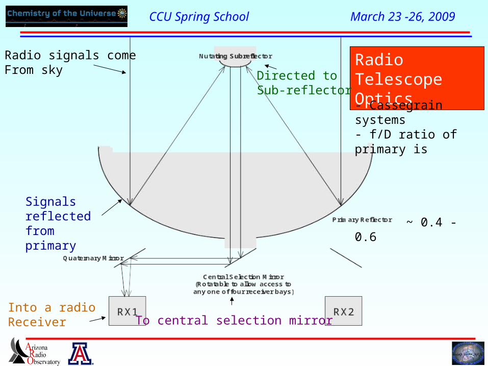
Radio signals comeFrom sky
Signals reflected from primary
Radio Telescope OpticsDirected to
Sub-reflector
To central selection mirrorInto a radioReceiver
- Cassegrain systems- f/D ratio of primary is ~ 0.4 -0.6
CCU Spring School March 23 -26, 2009
Dewar windowLens
Feedhorn
Coupler
Mixer
Bias
Isolator
HEMTamplifier
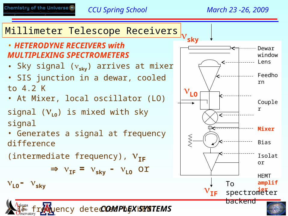
• HETERODYNE RECEIVERS withMULTIPLEXING SPECTROMETERS • Sky signal (sky) arrives at mixer
• SIS junction in a dewar, cooled to 4.2 K
• At Mixer, local oscillator (LO) signal (LO) is
mixed with sky signal • Generates a signal at frequency difference
(intermediate frequency), IF
IF = sky - LO or LO- sky
• IF frequency detected by HEMT amplifier • IF Signal sent to the spectrometer (Backend)• Not single signal but range IF 0.5 GHz =
sky 0.5 GHz
Millimeter Telescope Receivers
LO
sky
IF
To spectrometer backend
COMPLEX SYSTEMS
CCU Spring School March 23 -26, 2009
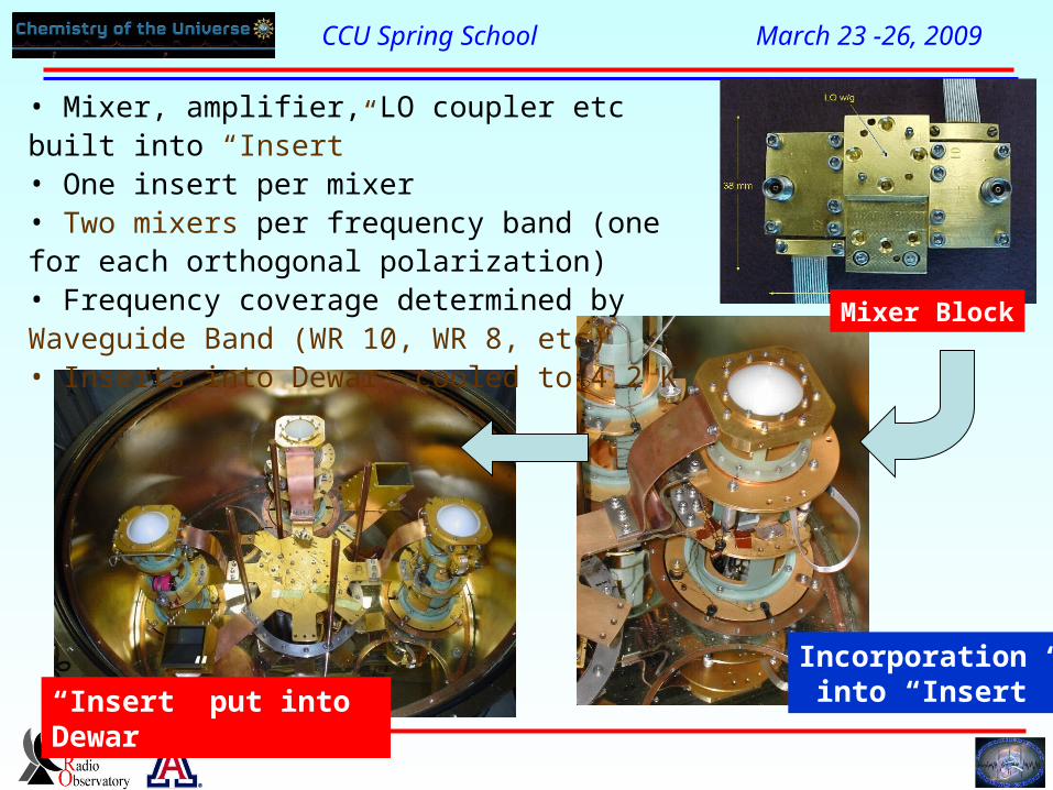
Mixer Block
• Mixer, amplifier, LO coupler etc built into “Insert”• One insert per mixer• Two mixers per frequency band (one for each orthogonal polarization)• Frequency coverage determined by Waveguide Band (WR 10, WR 8, etc)• Inserts into Dewar; cooled to 4.2 K
Incorporation into “Insert”“Insert” put into Dewar

CCU Spring School March 23 -26, 2009
A Complete Receiver… Optics
Card Cage
Cryo linescabling
CCU Spring School March 23 -26, 2009
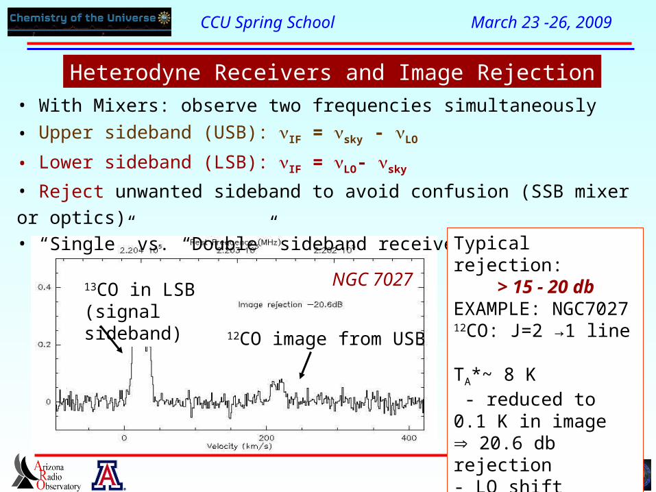
Heterodyne Receivers and Image Rejection
• With Mixers: observe two frequencies simultaneously
• Upper sideband (USB): IF = sky - LO
• Lower sideband (LSB): IF = LO- sky
• Reject unwanted sideband to avoid confusion (SSB mixer or optics)• “Single” vs. “Double” sideband receiver (SSB vs. DSB)
13CO in LSB (signal sideband)
12CO image from USB
NGC 7027
Typical rejection: > 15 - 20 db EXAMPLE: NGC702712CO: J=2 →1 line TA*~ 8 K - reduced to 0.1 K in image 20.6 dbrejection- LO shift

CCU Spring School March 23 -26, 2009
IF Systems at Radio Telescopes
• Radio Telescopes: MULTIPLEX ADVANTAGE• Simultaneously collect data over complete BW of IF Amplifier• Must have electronics to cleanly process IF signals
Frequency
steering
AOS
A,B,C
Filterbanks
Rx switch/
Total power/
Attenuators
IF System Block Diagram: SMT
Channel
steering
345Rx
490Rx
NewRx
1.5G
Rx
switch RightFlange
Rx
BE switch
1.5->5G
Converter5G
Rx
switch
Right Rx roomLeft Rx room
Computer room
• Mix IF signal down to base band• Send into spectrometer
CCU Spring School March 23 -26, 2009
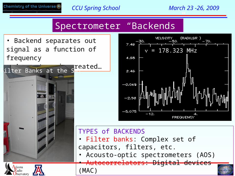
Spectrometer “Backends”
TYPES of BACKENDS• Filter banks: Complex set of capacitors, filters, etc.• Acousto-optic spectrometers (AOS)• Autocorrelators: Digital devices (MAC)
• Backend separates out signal as a function of frequency A spectrum is created…
= 178.323 MHz
Filter Banks at the SMT

CCU Spring School March 23 -26, 2009
Filter Card Block Diagram(one channel)
MuxBPF
Zero DAC
Square law detector
Integrator
Filter Card for 16 channels:1 MHz resolution filters
CCU Spring School March 23 -26, 2009
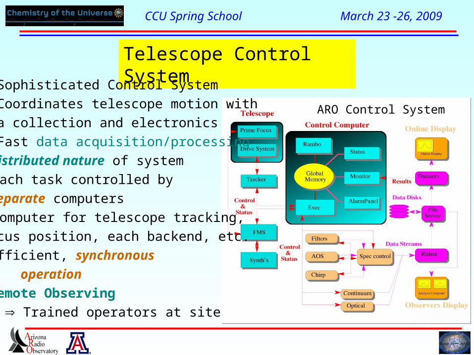
Telescope Control System
• Sophisticated Control System• Coordinates telescope motion with
data collection and electronics• Fast data acquisition/processing• Distributed nature of system Each task controlled by
separate computers Computer for telescope tracking,
focus position, each backend, etc.• Efficient, synchronous
operation• Remote Observing
Trained operators at site
ARO Control System
CCU Spring School March 23 -26, 2009
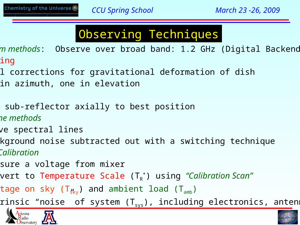
• Continuum methods: Observe over broad band: 1.2 GHz (Digital Backend)1) Pointing - Small corrections for gravitational deformation of dish - one in azimuth, one in elevation 2) Focus - Move sub-reflector axially to best position•Spectral Line methods - Observe spectral lines - Background noise subtracted out with a switching technique•Telescope Calibration - Measure a voltage from mixer
- Convert to Temperature Scale (TR*) using “Calibration Scan”
- Voltage on sky (Tsky) and ambient load (Tamb)
- Intrinsic “noise” of system (Tsys), including electronics, antenna, sky
Observing Techniques

CCU Spring School March 23 -26, 2009
Pointing scan or continuum 5-point: done on planet Jupiter
Establish pointing constants in az and elv
CCU Spring School March 23 -26, 2009
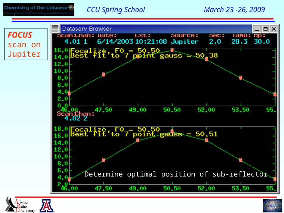
FOCUS scan on Jupiter
Determine optimal position of sub-reflector
CCU Spring School March 23 -26, 2009
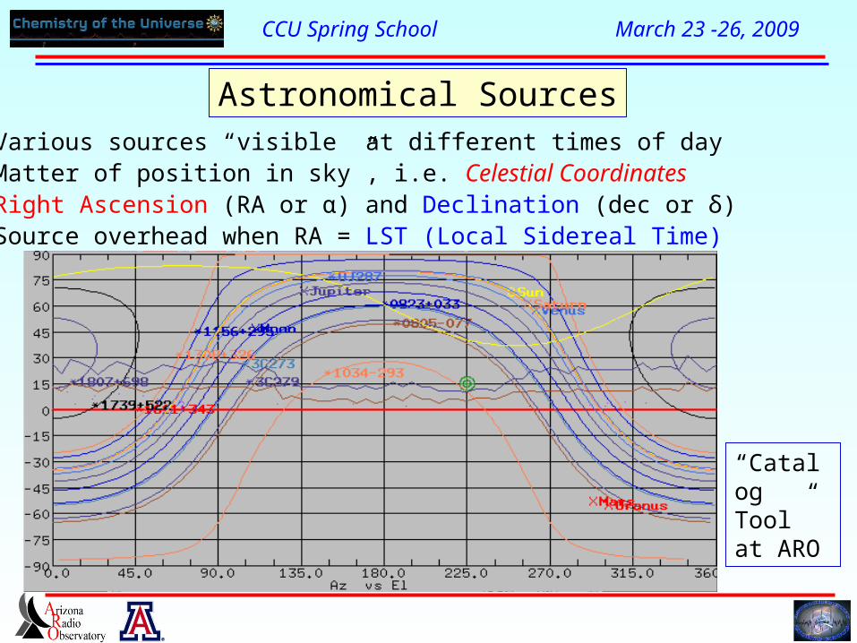
• Various sources “visible” at different times of day• Matter of position in sky”, i.e. Celestial Coordinates• Right Ascension (RA or α) and Declination (dec or δ)• Source overhead when RA = LST (Local Sidereal Time)
Astronomical Sources
“Catalog Tool”at ARO

CCU Spring School March 23 -26, 2009
• Position switching Switch telescope position between the source and blank sky
(“off position”: 10-30 arcmin away in azimuth) Subtract “(ON – OFF)/OFF” to remove background Calibrate the intensity scale (voltage) by doing a
“Cal scan” :Tscale=TA*( in K)
• Beam-switching
Nutate sub-reflector to get ON/OFF positions
Also begin with Cal Scan • Frequency switching
Change frequency of LO ± 1-2 MHz
Spectral Line Techniques
Molecular cloud
Blank sky
• (ON-OFF)/OFF and calibration all done instantly in software

CCU Spring School March 23 -26, 2009
• Data obtained immediately calibrated with background subtracted
• Background given by SYSTEM TEMPERATURE (Tsys)
• Tsys changes with time
• Tsys ~ 150 – 250 K with new ALMA 3 mm rxr at 12 m
• Spectral Line Intensity (TR*) ~ 0.001 – 10 K
• Want background subtracted• No further reduction needed• Only cosmetic:
baseline subtraction, “bad channels”, etc)• Look at data and ON-LINE decisions• Change frequency, source, receiver, etc. Optimize data return• Flexibility for new discoveries
Data Calibration and Intensity Scales

CCU Spring School March 23 -26, 2009
Sensitivity Limits:
Trms 2Tsys
spec t int
• Tsys = system temperature
• For a noise level of 0.5 mK, signal
average for ~100 hours (Tsys ~ 300 K)
• Requires telescope systems to be very stable over long periods of time can be accomplished with ARO
rms = 2mk at 12+ hrs
rms = 1 mK at 25 hrs
rms = 0.5 mK at 100 hrs
Extensive Signal-Averaging
• Collect data over 5-6 min as a single “scan” with a scan number• Written to computer disk• Average many scans for high S/N
Radiometer Equation

CCU Spring School March 23 -26, 2009
Spectrum after 15 hoursTrms = 0.0014 KMOSTLY NOISE
Spectrum after 30 hoursrms = 0.0010 KMAYBE A LINE ???
Spectrum after 60 hoursrms = 0.0007 K
LINES APPEAR
• Searching for KCN: new molecule
• J(Ka,Kc) = 16(0,16) 15(0,15)
at 150.0433 GHz
Signal Averaging: An Illustration
IRC+10216
KCN UU
CCU Spring School March 23 -26, 2009
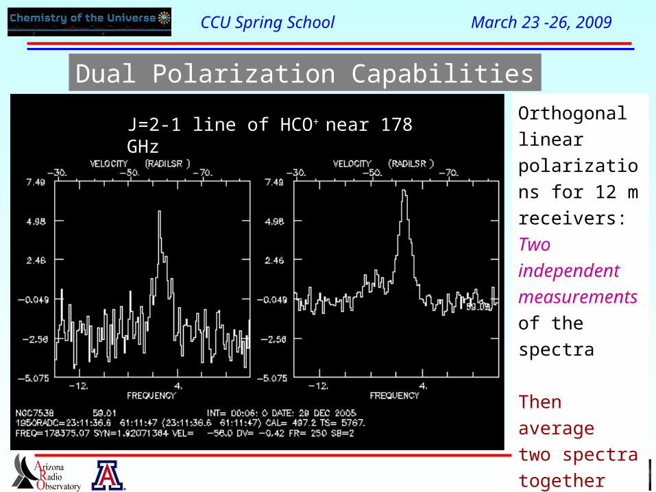
Dual Polarization Capabilities
J=2-1 line of HCO+ near 178 GHzOrthogonal
linear
polarizations
for 12 m
receivers: Two
independent
measurements
of the spectra
Then average
two spectra
together for
increased S/N
CCU Spring School March 23 -26, 2009
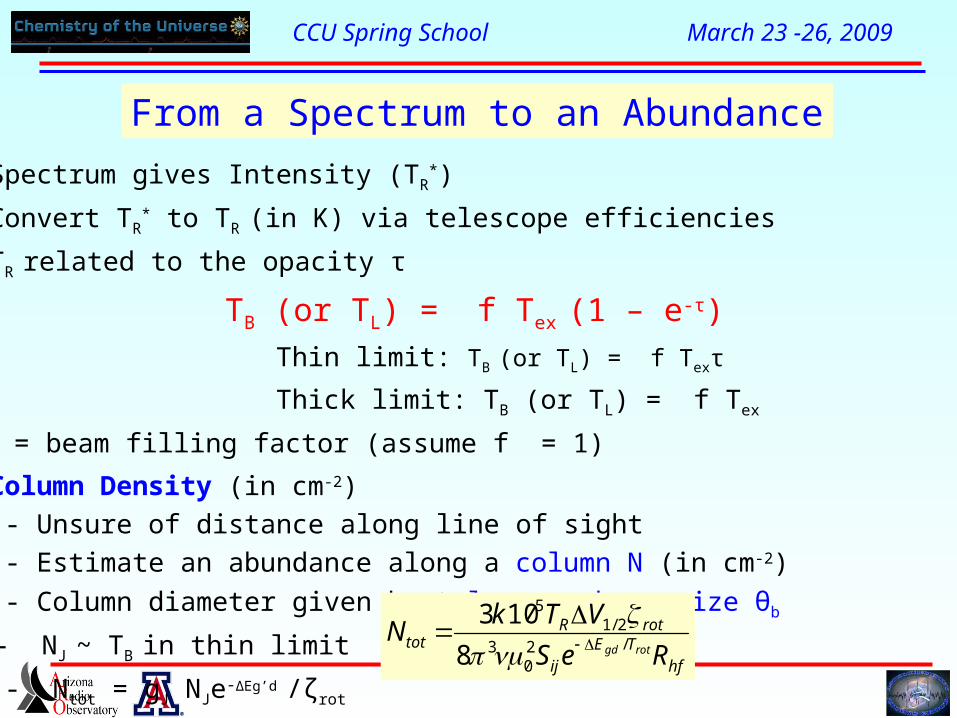
• Spectrum gives Intensity (TR*)
• Convert TR* to TR (in K) via telescope efficiencies
• TR related to the opacity τ
TB (or TL) = f Tex (1 – e-τ)
Thin limit: TB (or TL) = f Texτ
Thick limit: TB (or TL) = f Tex
• f = beam filling factor (assume f = 1)
• Column Density (in cm-2)
- Unsure of distance along line of sight
- Estimate an abundance along a column N (in cm-2)
- Column diameter given by telescope beam size θb
- NJ ~ TB in thin limit
- Ntot = gJ NJe-ΔEg’d /ζrot
From a Spectrum to an Abundance
hfTE
ij
rotRtot
ReS
VTkN
rotgd /20
32/1
5
8
103

CCU Spring School March 23 -26, 2009
Trot = 27 ± 8 KNtot = 1.1 ± 0.4 x1011 cm-2
KCN/H2 ~ 3 x10-11
Rotational Diagrams• Measure many transitions
• More accurate picture of abundance and excitation
• Population in the levels governs the intensity of the transitions
• By considering multiple transitions, column density (abundance) and temperature governing level population can be derived• Create “Rotational Diagram”• Also model with more sophisticated excitation code: LVG, Monte Carlo formalism, etc.

CCU Spring School March 23 -26, 2009
Line Profiles Contain Kinematic Information

CCU Spring School March 23 -26, 2009
1.4
1.2
1.0
0.8
0.6
0.4
0.2
0.0
TR
* (K)
232000231800231600231400231200231000Frequency (MHz)
13C
S
OC
S
C2H
3CN
C2H
3CN
C2H
3CN
CH
3CH
O +
C2H
3CN
CH
3CH
O +
C2H
5CN
C2H
3CN
C2H
3CN
HC
OO
CH
3 +
C2H
3CN
C2H
3CN
C2H
5CN
C2H
5CN
C2H
5CN
C2H
5CN
HC
OO
CH
3
HC
OO
CH
3
HC
OO
CH
3
HC
OO
CH
3
HC
OO
CH
3
CH
3CH
O
C2H
3CN
+ C
2H5C
N
C2H
5OH
C2H
5OH
+ (C
H2O
H) 2
CH
3CH
O
C2H
5OH
CH
3NH
2
HN
CO
CH
3CH
O
CH
3CH
O
HC
OO
H
C2H
5OH
(CH
3)2O
(CH
3)2O
NH
2CH
O
37 Indentified Features35 Unidentified Features~6 lines per 100 km/sTRMS = 0.003 K (theoretical)
U
U U
U U
U
U
U
U
CCU Spring School March 23 -26, 2009
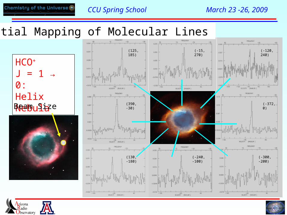
(125, 185)
(390, -30)
(130, -180)
(-15, 270)
(-240, -100)
(-120, 240)
(-372, 0)
(-300, -200)
HCO+ J = 1 → 0:Helix Nebula
Spatial Mapping of Molecular Lines
Beam Size
CCU Spring School March 23 -26, 2009
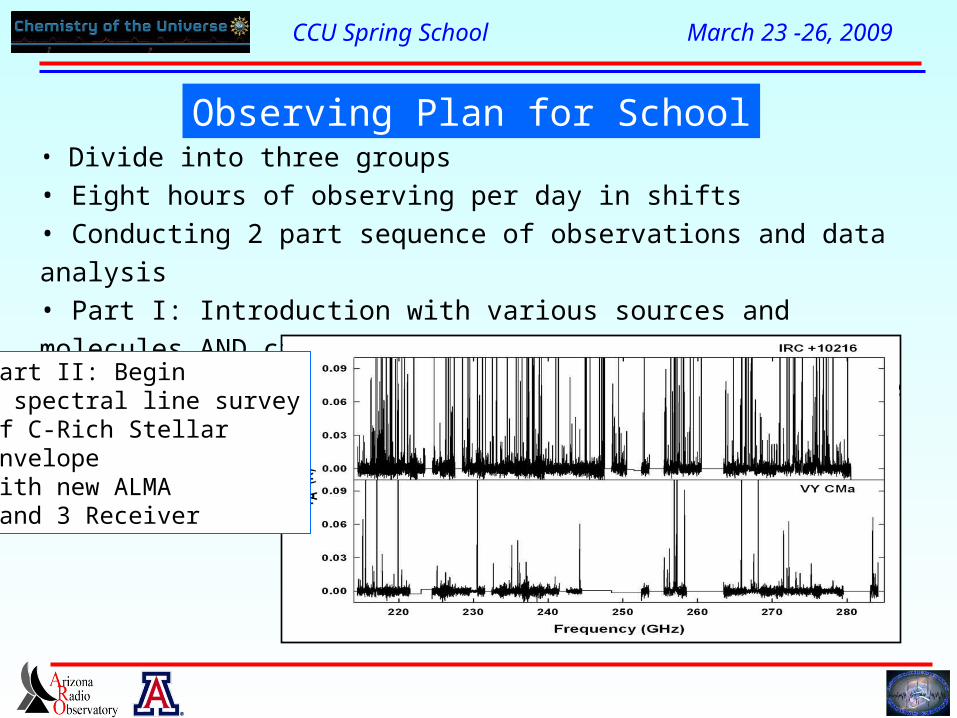
Observing Plan for School• Divide into three groups• Eight hours of observing per day in shifts• Conducting 2 part sequence of observations and data analysis• Part I: Introduction with various sources and molecules AND calculations• Part II: Real observations could lead to publishable results
Part II: Begin a spectral line surveyof C-Rich StellarEnvelopewith new ALMABand 3 Receiver
CCU Spring School March 23 -26, 2009
Watch out for the Skunk !


