

CF-1 Bank Hapoalim Jun-2001
Zvi Wiener
02-588-3049http://pluto.mscc.huji.ac.il/~mswiener/zvi.html
Computational Finance

CF1 slide 2Zvi Wiener
Plan1. Introduction, deterministic methods.2. Stochastic methods.3. Monte Carlo I.4. Monte Carlo II.5. Advanced methods for derivatives.
Other topics:queuing theory, floaters, binomial trees, numeraire, ESPP, convertible bond, DAC, ML-CHKP.
CF1 slide 3Zvi Wiener
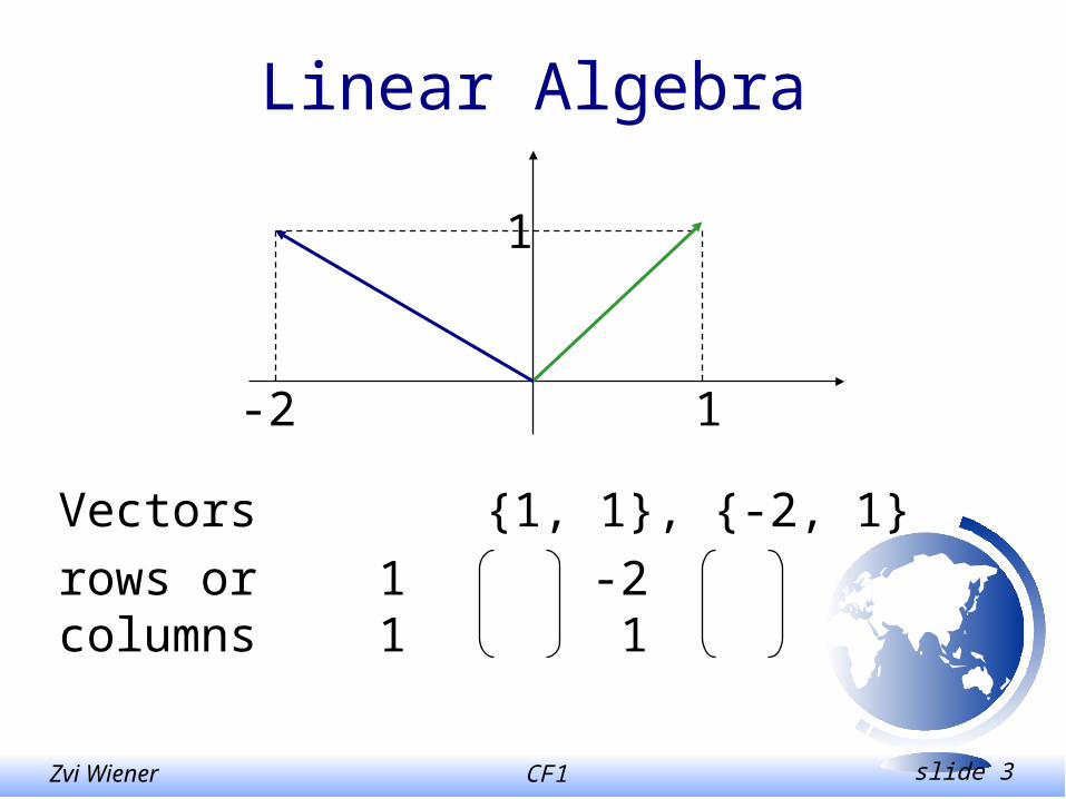
Linear Algebra
-2 1
1
Vectors {1, 1}, {-2, 1}
rows or 1 -2columns 1 1

CF1 slide 4Zvi Wiener
Linear Algebra

CF1 slide 5Zvi Wiener
Basic Operations
1 2 3
2 + -1 = 1
-2 1 -1
1 3
3 2 = 6
2 6

CF1 slide 6Zvi Wiener
Linear Algebra
vector
3
2
1
x
x
x
x Vectors form a linear space.
3
2
1
x
x
x
x
33
22
11
yx
yx
yx
yx Zero vector
Scalar multiplication

CF1 slide 7Zvi Wiener
Linear Algebra
matrix
333231
232221
131211
aaa
aaa
aaa
AMatrices alsoform a linearspace.
Zero matrix
000
000
000
Unit matrix
100
010
001

CF1 slide 8Zvi Wiener
Linear Algebra
Matrix can operate on a vector
3
2
1
333231
232221
131211
x
x
x
aaa
aaa
aaa
Ax
333232131
323222121
313212111
xaxaxa
xaxaxa
xaxaxa
How does zero matrix operate?
How does unit matrix operate?

CF1 slide 9Zvi Wiener
Linear Algebra
Transposition of a matrix
A symmetric matrix is A=AT
for example a variance-covariance matrix.
333231
232221
131211
aaa
aaa
aaa
A
332313
322212
312111
aaa
aaa
aaa
AT

CF1 slide 10Zvi Wiener
Linear Algebra
Matrix multiplication
333323321331323322321231313321321131
332323221321322322221221312321221121
331323121311321322121211311321121111
bababababababababa
bababababababababa
bababababababababa
333231
232221
131211
333231
232221
131211
bbb
bbb
bbb
aaa
aaa
aaa
AB

CF1 slide 11Zvi Wiener
Scalar Product
i
iibaba
332211
3
2
1
321 ,, bababa
b
b
b
aaa
a is orthogonal to b if ab = 0
CF1 slide 12Zvi Wiener
Linear Algebra
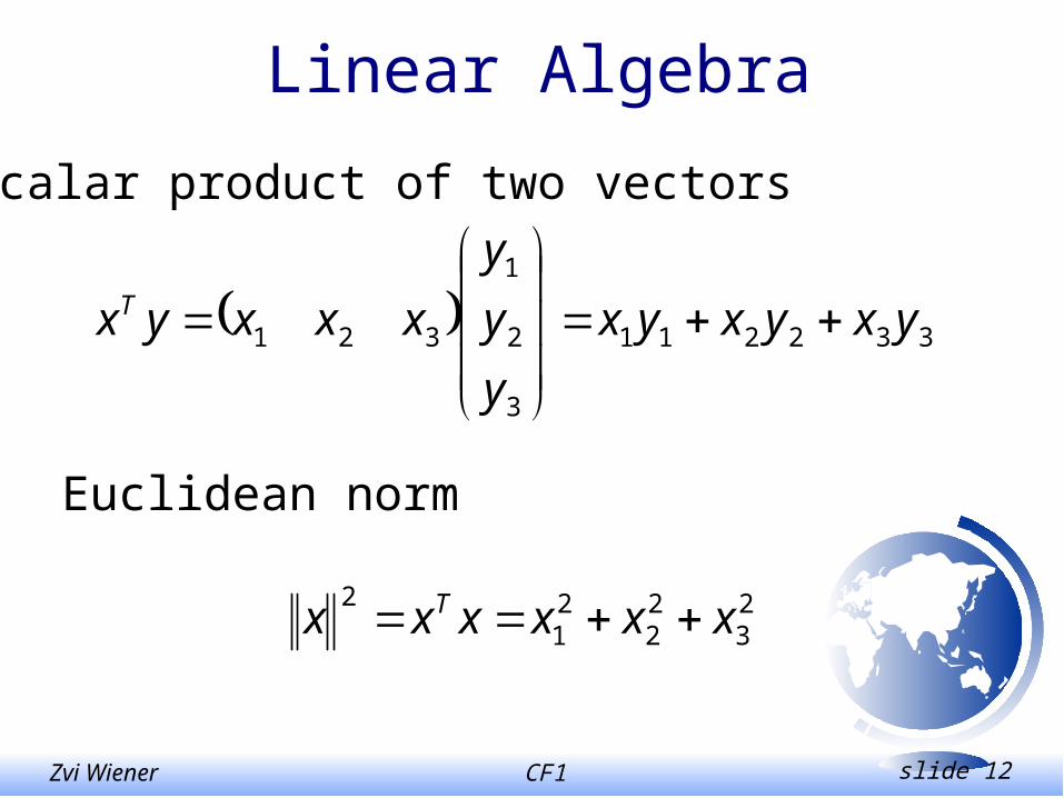
Scalar product of two vectors
332211
3
2
1
321 yxyxyx
y
y
y
xxxyxT
Euclidean norm
23
22
21
2xxxxxx T
CF1 slide 13Zvi Wiener
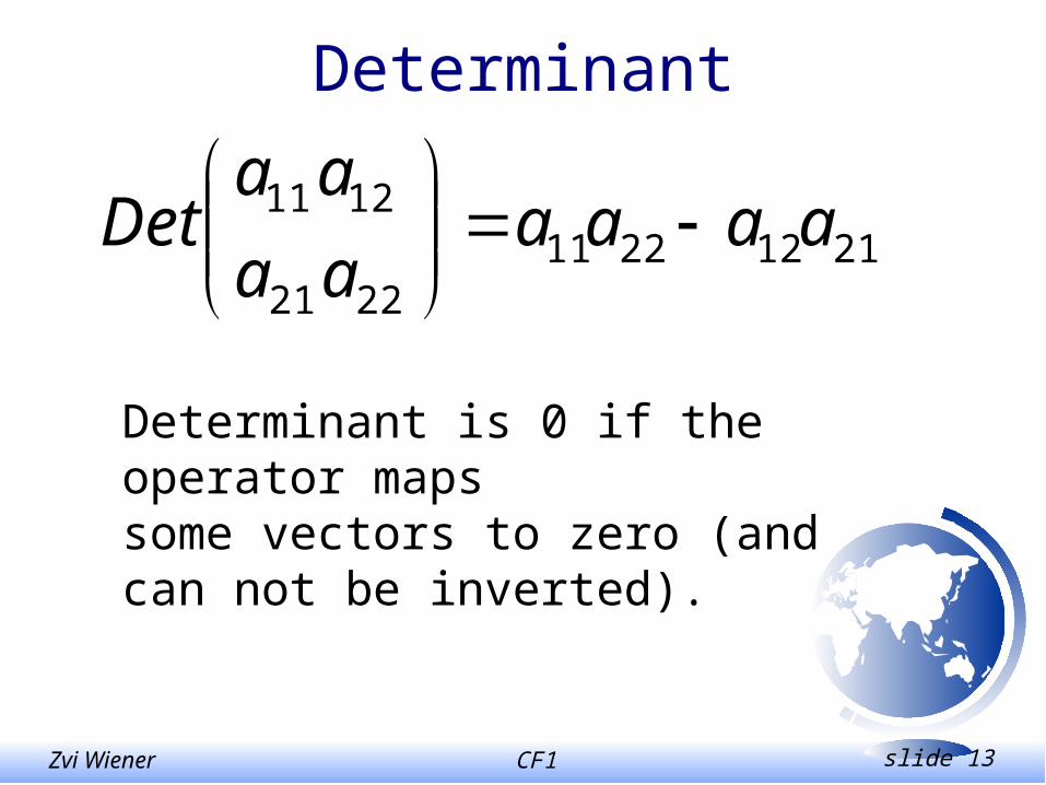
Determinant
211222112221
1211 aaaaaa
aaDet
Determinant is 0 if the operator mapssome vectors to zero (and can not be inverted).

CF1 slide 14Zvi Wiener
Linear Algebra
• Matrix multiplication corresponds to a
consecutive application of each operator.
• Note that it is not commutative! ABBA.
• Unit matrix does not change a vector.
• An inverse matrix is such that AA-1=I.

CF1 slide 15Zvi Wiener
Linear Algebra
• Determinant of a matrix ...
• A matrix can be inverted if det(A)0
• Rank of a matrix
• Matrix as a system of linear equations Ax=b.
• Uniqueness and existence of a solution.
• Trace tr(A) – sum of diagonal elements.
CF1 slide 16Zvi Wiener
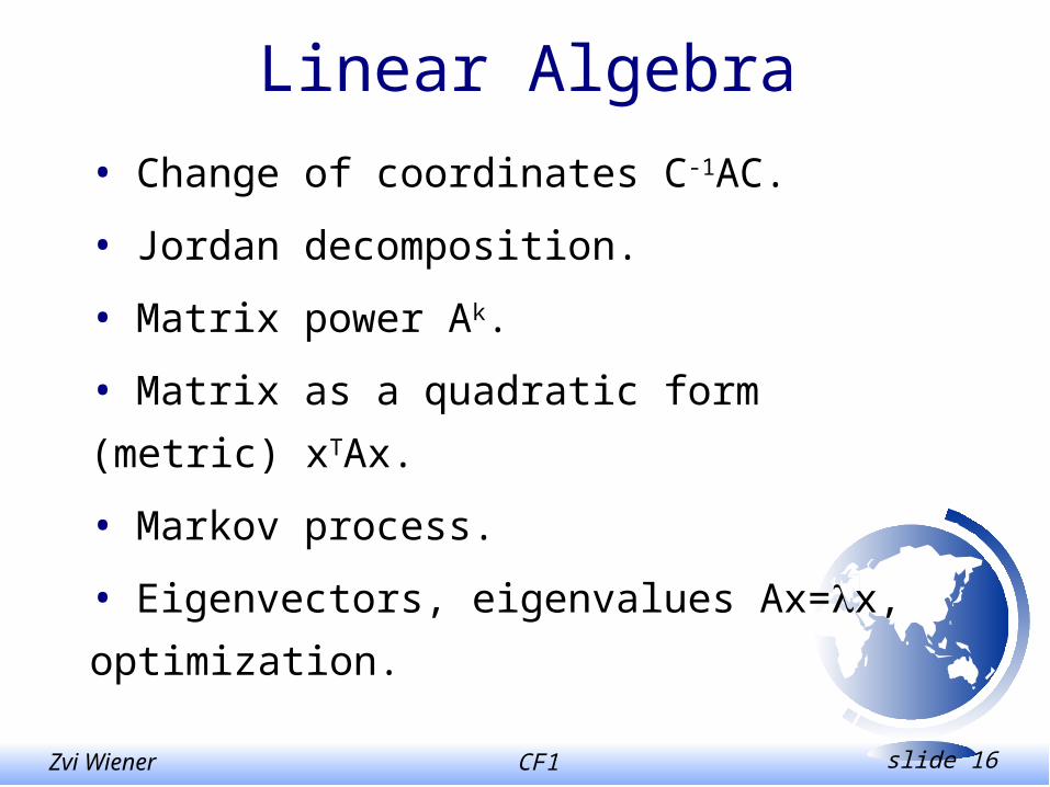
Linear Algebra
• Change of coordinates C-1AC.
• Jordan decomposition.
• Matrix power Ak.
• Matrix as a quadratic form (metric) xTAx.
• Markov process.
• Eigenvectors, eigenvalues Ax=x,
optimization.

CF1 slide 17Zvi Wiener
Problems
Check how the following matrices act on vectors:
00
01
10
01
10
01
cossin
sincos
01
10
01
10
CF1 slide 18Zvi Wiener
Simple Exercises
• Show an example of ABBA.
• Construct a matrix that inverts each vector.
• Construct a matrix that rotates a two dimensional vector by an angle .
• Construct a covariance matrix, show that it is symmetric.
• What is mean and variance of a portfolio in matrix terms?

CF1 slide 19Zvi Wiener
Examples
• Credit rating and credit dynamics.
• Variance-covariance model of VaR.
• Can the var-covar matrix be inverted
• VaR isolines (the ovals model).
• Prepayment model based on types of clients.
• Finding a minimum of a function.

CF1 slide 20Zvi Wiener
Calculus
• Function of one and many variables.
• Continuity in one and many directions.
• Derivative and partial derivative.
• Gradient and Hessian.
• Singularities, optimization, ODE, PDE.
CF1 slide 21Zvi Wiener
x
$
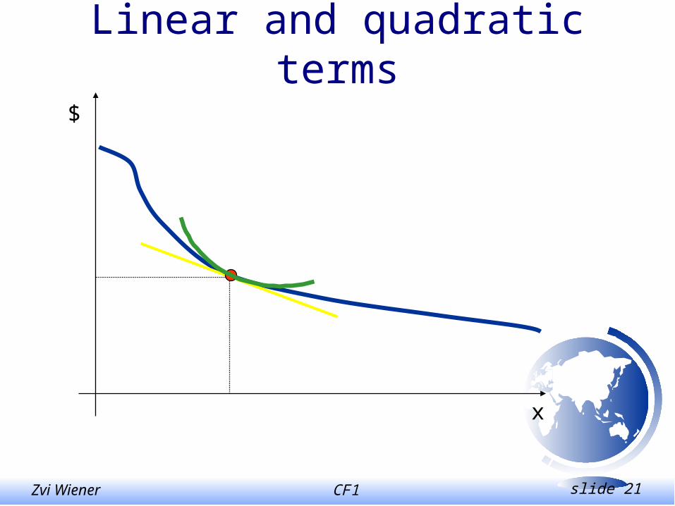
Linear and quadratic terms

CF1 slide 22Zvi Wiener
Taylor series
22
2)(")(')()( xo
xxfxxfxfxxf
2222
22
),(),(
yxoy
gyxgx
g
ygxgyxgyyxxg
yyxyxx
yx
2)("
2
1)(')()( xoxxFxxxFxFxxF T

CF1 slide 23Zvi Wiener
Variance-Covariance
),...,,()( 21 nxxxVxV
nnn
n
n
1
2221
112111
,

CF1 slide 24Zvi Wiener
Variance-Covariance
nx
V
x
V
xV 1
)('Gradient vector:

CF1 slide 25Zvi Wiener
Variance-Covariance
2)("2
1)(')()( xxVxxVxVxxV
2)("2
1)(')( xxVxxVxV

CF1 slide 26Zvi Wiener
Variance-Covariance
22
)(")(' xE
xVxVxEVE
"2
1' VtrVVE T
'' VVV T

CF1 slide 27Zvi Wiener
Variance-Covariance
For a short time period , the changes in the value are distributed approximately normal with the following mean and variance:
''
"2
1'
2 VVV
VtrVVE
T
T

CF1 slide 28Zvi Wiener
Variance-Covariance
Then VaR can be found as:
)(33.2)(%,1 VVVVaR
''33.2"2
1' VVVtrV TT

CF1 slide 29Zvi Wiener
Weighted Variance covariance
Volatility estimate on day i based on last M days.
i
Mijj RR
Mt 1
2)()1(
1
i
jj
ji RRt
2)(1

CF1 slide 30Zvi Wiener
Weighted Variance covariance
Covariance on day i based on last M days.
i
Mijjj RRRR
Mt 1221112 ))((
)1(
1
It is important to check that the resulting
matrix is positive definite!

CF1 slide 31Zvi Wiener
Positive Quadratic Form
For every vector x a we have x.A.x > 0
Only such a matrix can be used to define a
norm.
For example, this matrix can not have
negative diagonal elements. Any variance-
covariance matrix must be positive.

CF1 slide 32Zvi Wiener
Positive Quadratic Form
Needs["LinearAlgebra`MatrixManipulation`"];
ClearAll[ positiveForm ];
positiveForm[ a_?MatrixQ ] := Module[{aa, i},
aa = Table[
Det[ TakeMatrix[ a, {1, 1}, {i, i}] ],
{i, Length[a]}];
{ aa, If[ Count[ aa, t_ /; t < 0] > 0, False, True]}
];

CF1 slide 33Zvi Wiener
Stochastic (transition) Matrix
Used to define a Markov chain (only the last state matters).
A matrix P is stochastic if it is non-negative and sum of elements in each line is 1.
One can easily see that 1 is an eigenvalue of any stochastic matrix.
What is the eigenvector?

CF1 slide 34Zvi Wiener
Markov chain
• credit migration
• prepayment and freezing of a program
CF1 slide 35Zvi Wiener
Stochastic (transition) Matrix
Theorem: P0 is stochastic iff (1,1,…1) is an eigenvector with an eigenvalue 1 and this is the maximal eigenvalue.
If both P and PT are stochastic, then P is called double stochastic.

CF1 slide 36Zvi Wiener
Cholesky decomposition
The Cholesky decomposition writes a symmetric positive definite matrix as the product of an upper triangular matrix and its transpose.
In MMA CholeskyDecomposition[m]
CF1 slide 37Zvi Wiener
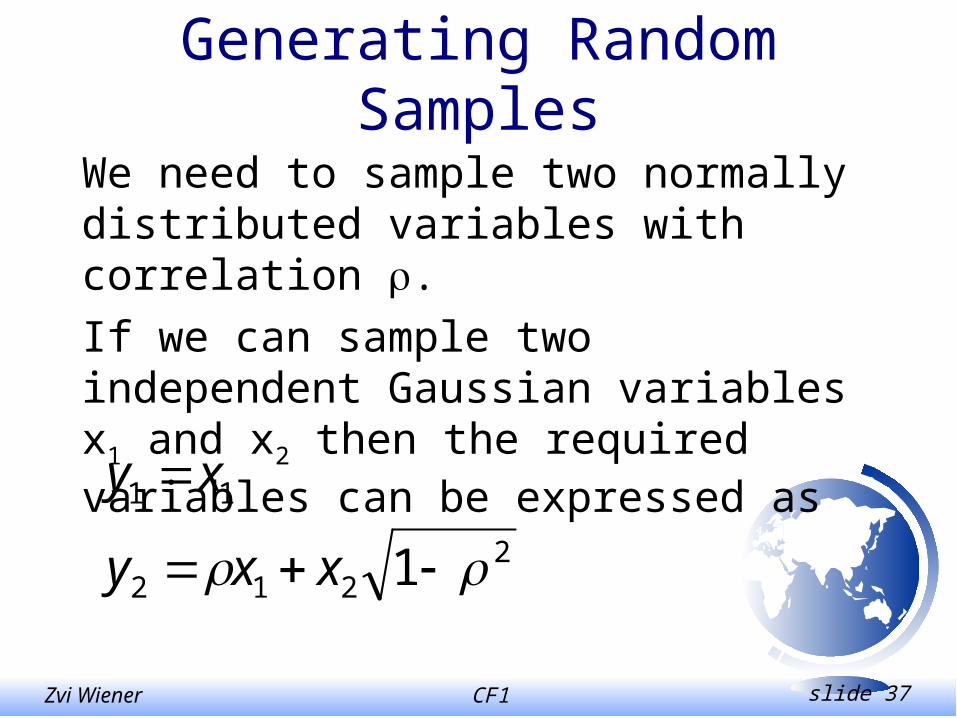
Generating Random Samples
We need to sample two normally distributed variables with correlation .
If we can sample two independent Gaussian variables x1 and x2 then the required variables can be expressed as
2212
11
1
xxy
xy

CF1 slide 38Zvi Wiener
Generating Random Samples
We need to sample n normally distributed variables with correlation matrix ij, ( >0).
Sample n independent Gaussian variables x1…xn.
n
kkiki xay
1
xAy .
AAAanda Tn
kik ,,1
1
2
CF1 slide 39Zvi Wiener
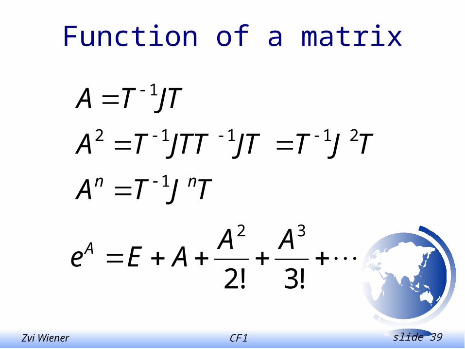
Function of a matrix
!3!2
32 AAAEeA
TJTA
TJTJTJTTTA
JTTA
nn 1
21112
1

CF1 slide 40Zvi Wiener
ODE
Axdt
dx 00 )( xtx
0)( 0)( xetx ttA

CF1 slide 41Zvi Wiener
ODE
)(tfAxdt
dx 00 )( xtx
t
t
tAttA dtfexetx0
0 )()( )(0
)(

CF1 slide 42Zvi Wiener
Bisection method
If the function is monotonic, e.g. implied vol.
x
f

CF1 slide 43Zvi Wiener
Newton’s method
x
f
x1x2x3

CF1 slide 44Zvi Wiener
Solve and FindRoot
Solve[ 0 = = x2- 0.8x3- 0.3, {x}]
{{x -> -0.467297}, {x ->0.858648 -0.255363*I}, {x -> 0.858648 + 0.255363*I}}
FindRoot[ x2 + Sin[x] - 0.8x3 - 0.3, {x, 0,1}]
{x -> 0.251968}

CF1 slide 45Zvi Wiener
Max, min of a multidimensional function
• Gradient method
• Solve a system of equations (both derivatives)
-1
-0.5
0
0.5
1-1
-0.5
0
0.5
1
0
0.5
1
-1
-0.5
0
0.5
1

CF1 slide 46Zvi Wiener
-1 -0.5 0 0.5 1-1
-0.5
0
0.5
1
Gradient method

CF1 slide 47Zvi Wiener
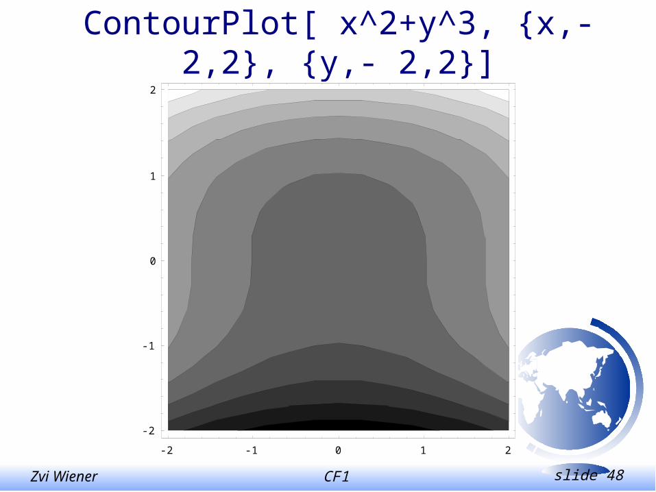
Level curve of a multivariate function
ContourPlot[ x^2+y^3, {x,-2,2}, {y,- 2,2}]
ContourPlot[ x^2+y^3, {x,-2,2}, {y,- 2,2}], Contours->{1 ,-0.5}, ContourShading->False];
CF1 slide 48Zvi Wiener
ContourPlot[ x^2+y^3, {x,-2,2}, {y,- 2,2}]
-2 -1 0 1 2
-2
-1
0
1
2

CF1 slide 49Zvi Wiener
ContourPlot[ x^2+y^3, {x,-2,2}, {y,- 2,2}], Contours->{1 ,-0.5}, ContourShading->False];
-2 -1 0 1 2
-2
-1
0
1
2

CF1 slide 50Zvi Wiener
Example
Consider a portfolio with two risk factors and benchmark duration of 6M.
The VaR limit is 3 bp. and you have to make two decisions:
a – % of assets kept in spread products
q – duration mismatch
we assume that all instruments (both treasuries and spread) have the same duration T+q months.

CF1 slide 51Zvi Wiener
q - durationmismatch
Contour Levels of VaR (static)
0 0.2 0.4 0.6 0.8 1
-6
-4
-2
0
2
4
6
a (% of spread)

CF1 slide 52Zvi Wiener
0 0.2 0.4 0.6 0.8 1
-6
-4
-2
0
2
4
6
q - durationmismatch
a (% of spread)
position
VaR=2 bp
VaR=3 bp

CF1 slide 53Zvi Wiener
0 0.2 0.4 0.6 0.8 1
-6
-4
-2
0
2
4
6
q - durationmismatch
a (% of spread)
In order to reducerisk one can increase duration(in this case).

CF1 slide 54Zvi Wiener
0 0.2 0.4 0.6 0.8 1
-6
-4
-2
0
2
4
6
What we can do using limits
VaR = 6 bp

CF1 slide 55Zvi Wiener
0 0.2 0.4 0.6 0.8 1
-0.2
-0.1
0
0.1
0.2
spread %
duration mismatch (yr)
Position 2M, and10% spread5% weekly VaR=2.2 bp
weekly VaR limit 3 bp

CF1 slide 56Zvi Wiener
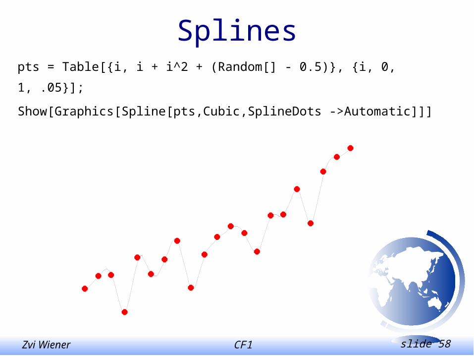
Splines
x1 x2 x3 … xn

CF1 slide 57Zvi Wiener
Splines<<Graphics`Spline`
pts = {{0, 0}, {1, 2}, {2, 3}, {3, 1}, {4, 0}}
Show[
Graphics[
Spline[pts, Cubic, SplineDots -> Automatic]]]
CF1 slide 58Zvi Wiener
Splinespts = Table[{i, i + i^2 + (Random[] - 0.5)}, {i, 0, 1, .05}];
Show[Graphics[Spline[pts,Cubic,SplineDots ->Automatic]]]

CF1 slide 59Zvi Wiener
Fitting datadata = Table[7*x + 3 + 10*Random[], {x, 10}];
f[x_] := Evaluate[Fit[data, {1, x}, x]]
Needs["Graphics`Graphics`"]
DisplayTogether[
ListPlot[data, PlotStyle -> {AbsolutePointSize[3],
RGBColor[1, 0, 0]}],
Plot[f[x], {x, 0, 10}, PlotStyle -> RGBColor[0, 0, 1]]
];

CF1 slide 60Zvi Wiener
Fitting data
2 4 6 8 10
20
40
60

CF1 slide 61Zvi Wiener
Fitting data
data = {{1.0, 1.0, .126}, {2.0, 1.0, .219},
{1.0, 2.0, .076}, {2.0, 2.0, .126}, {.1, .0, .186}};
ff[x_, y_] = NonlinearFit[data,
a*c*x/(1 + a*x + b*y), {x, y}, {a, b, c}];
ff[x, y]
nonlinear, multidimensional

CF1 slide 62Zvi Wiener
Orly - Nelson Siegel
50 100 150 200 250 300 350
0.125
0.13
0.135
0.14
0.145 MAKAM

CF1 slide 63Zvi Wiener
Numerical Differentiation
22
2)(")(')()( xo
xxfxxfxfxxf
22
2)(")(')()( xo
xxfxxfxfxxf
2)('2)()( xoxxfxxfxxf
xoxfx
xxfxxf
)('2
)()(

CF1 slide 64Zvi Wiener
Numerical Differentiation
22
2)(")(')()( xo
xxfxxfxfxxf
22
2)(")(')()( xo
xxfxxfxfxxf
22)(")()(2)( xoxxfxxfxfxxf
22
)(")()(2)(
xOxfx
xxfxfxxf

CF1 slide 65Zvi Wiener
Finite Differences
Typically equal time and S (or logS) steps.
time
S Following P. Wilmott, “Derivatives”

CF1 slide 66Zvi Wiener
Finite Differences
Time step tasset step S(i,k) node of the grid is t = T - kt, iS0 i I, 0 k K
assets value at each node is
note the direction of time!
),( tkTSiVV ki

CF1 slide 67Zvi Wiener
The Black-Scholes equation
Linear parabolic PDE
0)(2
12
222
rVS
VSrr
S
VS
t
Vf
Final conditions )(),( SPayoffTSV
Boundary conditions ...

CF1 slide 68Zvi Wiener
Transformation of BS
U
x
U2
2
.2
,
,12
4
1
,12
2
1
),(),(
2
2
2
2
rTt
eS
r
r
xUetSV
x
x

CF1 slide 69Zvi Wiener
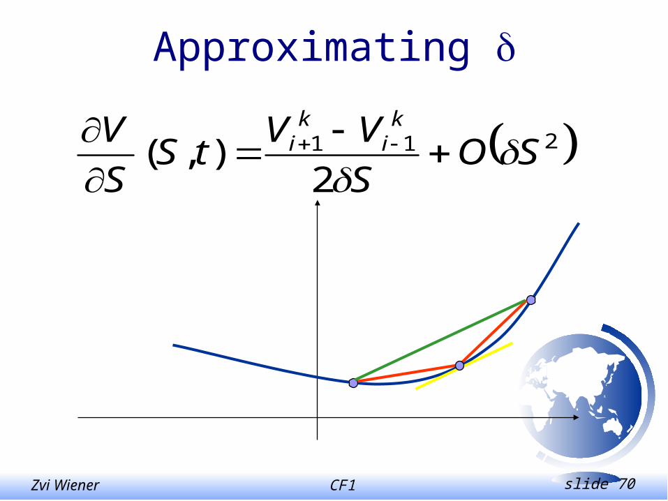
Approximating
h
tSVhtSV
t
Vh
),(),(lim
0
tOt
VVtS
t
V ki
ki
1
),(
CF1 slide 70Zvi Wiener
Approximating
211
2),( SO
S
VVtS
S
V ki
ki

CF1 slide 71Zvi Wiener
Approximating
22
112
2 2),( SO
S
VVVtS
S
V ki
ki
ki

CF1 slide 72Zvi Wiener
Bilinear Interpolation
A3A4
A2A1
V3V4
V2V1
4
1
4
1
jj
jjj
A
VA
V
Area of the rectangle

CF1 slide 73Zvi Wiener
Final conditions and payoffs
)(),( SPayoffTSV
)(0 SiPayoffVi
For example a European Call option
)0,(0 ESiMaxVi

CF1 slide 74Zvi Wiener
Boundary conditions Call
00 kV
For example a Call option
trkkI EeSIV
For large S the Call value asymptotes toS-Ee-r(T-t)

CF1 slide 75Zvi Wiener
Boundary conditions Put
trkk EeV 0
For example a Put option
0kIV
For large S
CF1 slide 76Zvi Wiener
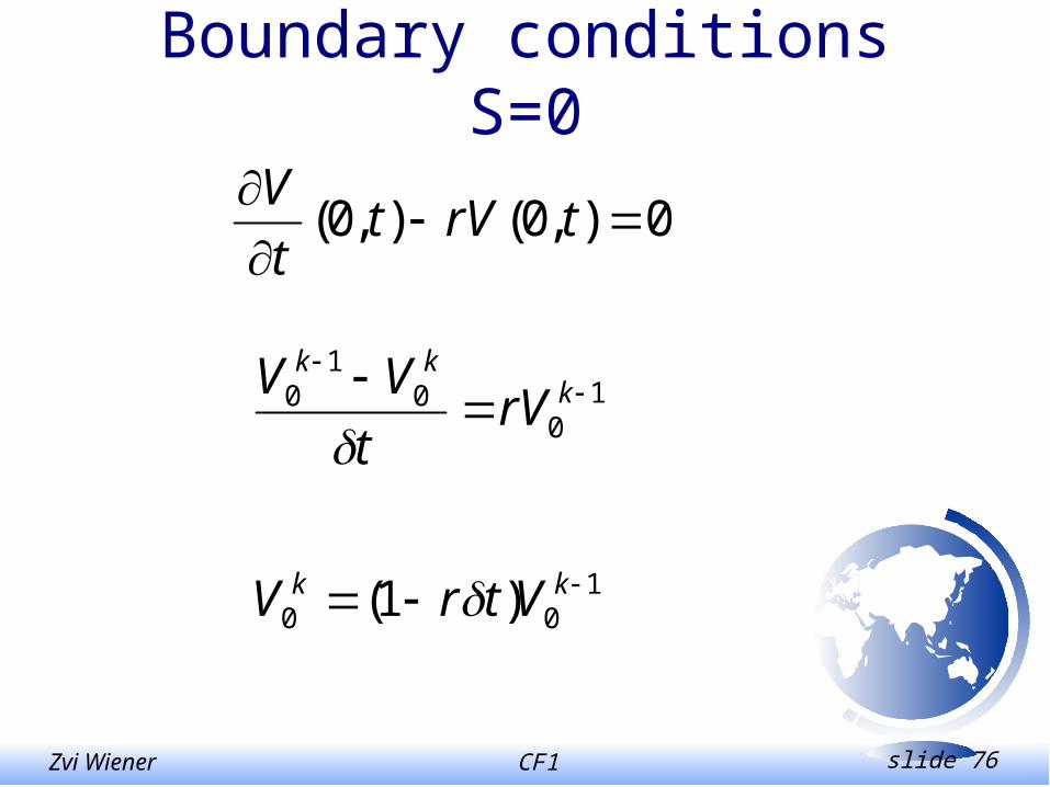
Boundary conditions S=0
0),0(),0(
trVtt
V
100 )1( kk VtrV
10
01
0
k
kk
rVt
VV
CF1 slide 77Zvi Wiener
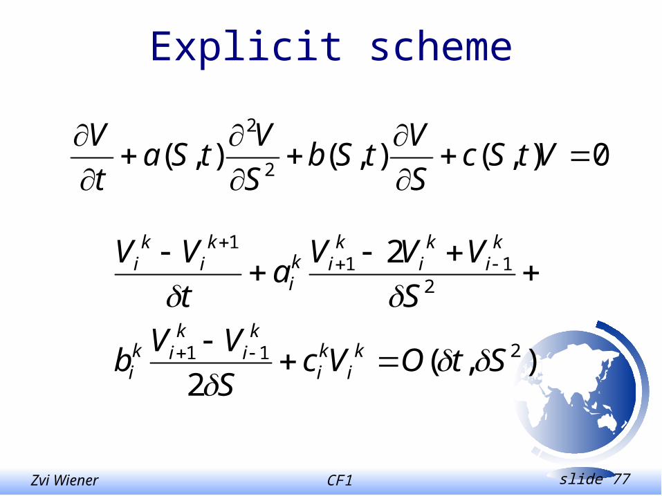
Explicit scheme
0),(),(),(2
2
VtScS
VtSb
S
VtSa
t
V
),(2
2
211
211
1
StOVcS
VVb
S
VVVa
t
VV
ki
ki
ki
kik
i
ki
ki
kik
i
ki
ki

CF1 slide 78Zvi Wiener
Explicit scheme
),(2
2
211
211
1
StOVcS
VVb
S
VVVa
t
VV
ki
ki
ki
kik
i
ki
ki
kik
i
ki
ki
ki
ki
ki
ki
ki
ki
ki VCVBVAV 11
1 )1(
Local truncation error 22 , SttO

CF1 slide 79Zvi Wiener
Explicit scheme
ki
ki
ki
ki
ki
ki
ki VCVBVAV 11
1 )1(
time
S
Value here is calculated
These values arealready known

CF1 slide 80Zvi Wiener
Explicit scheme
ki
ki
ki
ki
ki
ki
ki VCVBVAV 11
1 )1(
This equation is defined for 1i I-1,
for i=1 and i=I we use boundary conditions.

CF1 slide 81Zvi Wiener
Explicit scheme
ki
ki
ki
ki
ki
ki
ki VCVBVAV 11
1 )1(
For the BS equation (with dividends)
,2/))((
,)(
,2/))((
22
22
22
tiDriC
triB
tiDriA
ki
ki
ki

CF1 slide 82Zvi Wiener
Explicit scheme
Stability problems related to step sizes.
These relationships should guarantee stability.
Note that reducing asset step by half we must reduce the time step by a factor of four.
a
St
b
aS
2,
2 2

CF1 slide 83Zvi Wiener
Explicit scheme
Advantages
easy to program, hard to make a mistake
when unstable it is obvious
coefficients can be S and t dependent
Disadvantages
there are restrictions on time step, which may cause slowness.

CF1 slide 84Zvi Wiener
Implicit scheme
0),(),(),(2
2
VtScS
VtSb
S
VtSa
t
V
),(2
2
2111
11
11
2
11
1111
1
StOVcS
VVb
S
VVVa
t
VV
ki
ki
ki
kik
i
ki
ki
kik
i
ki
ki

CF1 slide 85Zvi Wiener
Implicit scheme
),(2
2
2111
11
11
2
11
1111
1
StOVcS
VVb
S
VVVa
t
VV
ki
ki
ki
kik
i
ki
ki
kik
i
ki
ki
11
11111
1 )1(
ki
ki
ki
ki
ki
ki
ki VCVBVAV

CF1 slide 86Zvi Wiener
Implicit scheme
time
S
Values here are calculated
This value is used
11
11111
1 )1(
ki
ki
ki
ki
ki
ki
ki VCVBVAV

CF1 slide 87Zvi Wiener
Crank-Nicolson scheme
),(2222
22
2
2
2
2
211
11
11
11
1
211
2
11
111
11
StOVc
Vc
S
VVb
S
VVb
S
VVVa
S
VVVa
t
VV
ki
kik
i
ki
ki
ki
ki
ki
ki
ki
ki
ki
ki
ki
ki
ki
ki
ki
ki
ki

CF1 slide 88Zvi Wiener
Crank-Nicolson scheme
ki
ki
ki
ki
ki
ki
ki
ki
ki
ki
ki
ki
VCVBVA
VCVBVA
11
11
11111
1
)1(
)1(

CF1 slide 89Zvi Wiener
Crank-Nicolson scheme
time
S
Values here are calculated
These values are used

CF1 slide 90Zvi Wiener
Crank-Nicolson scheme
0
0
0
10
10
000
1
01 10
11
11
12
12
11
11
11
12
12
12
12
11
11
kk
kI
kI
k
k
kI
kI
kI
kI
kk
kk VA
V
V
V
V
BA
CB
BA
CB
kkkR
kkL rvMvM 11
A general form of the linear equation is:
Note that M are tridiagonal!
CF1 slide 91Zvi Wiener
Crank-Nicolson scheme
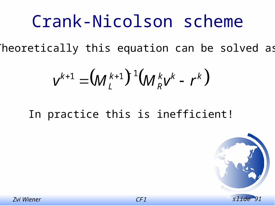
kkkR
kL
k rvMMv 111
Theoretically this equation can be solved as
In practice this is inefficient!
CF1 slide 92Zvi Wiener
LU decomposition
M is tridiagonal, thus M=LU, where L is
lower triangular, and U is upper triangular.
In fact L has 1 on the diagonal and one
subdiagonal only, U has a diagonal and one
superdiagonal.

CF1 slide 93Zvi Wiener
LU decomposition
Then in order to solve Mv=q
orLUv=q
We will solve
Lw=q
first, and then
Uv=w.

CF1 slide 94Zvi Wiener
LU decomposition
Very fast, especially when M is time
independent.
Disadvantages:
Needs a big modification for American options

CF1 slide 95Zvi Wiener
Other methods
• SOR successive over relaxation
• Douglas scheme
• Three time-level scheme
• Alternating direction method
• Richardson Extrapolation
• Hopscotch method
• Multigrid methods

CF1 slide 96Zvi Wiener
Multidimensional case
r
S
Fixed t layer
These values are usedto calculate space derivatives
Note additional boundary conditions.

CF1 slide 97Zvi Wiener
Geometrical Brownian Motion
SdBrSdtdS
)()( SpayoffEeoption neutralrisktTr

CF1 slide 98Zvi Wiener
Lognormal process
SdBrSdtdS
dBdtrSd
2)(log
2
tZtr N
eStS)1,0(
2
2)0()(

CF1 slide 99Zvi Wiener
Euler Scheme
SdBrSdtdS
)()1,0( tOtSZtrSS N

CF1 slide 100Zvi Wiener
Milstein Scheme
SdBrSdtdS
)()1(2
1 22)1,0(
22
)1,0(
tOtZS
tSZtrSS
N
N

CF1 slide 101Zvi Wiener
Stochastic Calculus
Standard Normal
Diffusion process
x z
dzexN 2
2
2
1)(
tdBtXdttXdX ),(),(
ABM tdBdtdX
GBM tXdBXdtdX

CF1 slide 102Zvi Wiener
Ito’s Lemma
tdBtXdttXdX ),(),(
22
2
),( dXX
FdX
X
Fdt
t
FtXdF
dt dXdt 0 0dX 0 dt

CF1 slide 103Zvi Wiener
)1,0(
2
2)0()(
Ztt
eXtX
)ln(XY
22
)(11
0 dXX
dXX
dtdY
tdBdtdY
2
2
)1,0(
2
2)0()( ZttYtY
tXdBXdtdX

CF1 slide 104Zvi Wiener
Siegel’s paradoxConsider two currencies X and Y. Define S an exchange rate (the number of units of currency Y for a unit of X).
The risk-neutral process for S is
tSXY SdBSdtrrdS )(
By Ito’s lemma the process for 1/S is
tSSXY dBS
dtS
rrS
d111 2

CF1 slide 105Zvi Wiener
Siegel’s paradoxThe paradox is that the expected growth rate of 1/S is not ry - rX, but has a correction term.


