

Changing cultures, changing environments: a novel means of investigating the effects of introducing
non-native species into past ecosystems
Jacqueline Pitta, Phillipa K. Gillinghama, Mark Maltbyb, Richard Stafforda and John R. Stewarta
a Department of Life and Environmental Sciences, Bournemouth University, Talbot Campus, Pooleb Department of Archaeology, Anthropology and Forensic Science, Bournemouth University, Talbot Campus, Poole
Keywords: Chicken; Domestication; Bayesian belief networks; Biotic interactions
Abstract: Descended from junglefowl of Asia and South-east Asia, the chicken was introduced into Europe
during the first millennium BCE. As one of the most recently domesticated species, it makes an excellent case
study for investigating the consequences of such introductions to past ecological communities. We present a
unique application of a novel ecological method to explore multiple past interspecies relationships. Analysing the
faunal record using a Bayesian belief network, which allows for the analysis of multiple interspecies relationships
simultaneously, indicates that the chicken has more affinity with other domestic birds rather than domestic
mammals in terms of species interactions. We find that the introduction of the chicken affected fox, partridge,
pigeon and rat, but the success of the chicken was most affected by responses to abiotic variables, rather than
biotic interactions. As the method is not limited to environmental variables, we also examined the effect of
recovery method and demonstrate that sieving would enhance the frequency of small animal remains recovered
from archaeological sites.
1. Introduction: Relationships between different species, otherwise termed inter-specific interactions, can be
both positive and negative. Interactions usually take the form of competition, predation, herbivory, and symbiosis
(Lang and Benbow 2013). Symbiosis, literally meaning ‘living-together’, encompasses commensalism,
amensalism, parasitism and mutualism, whereby only the latter is a mutually beneficial relationship and is not
necessarily equally so (Parmentier and Michel 2013). Within ecological communities these relationships become
established over time but can be disrupted by environmental change or by the introduction of non-native species.
Introducing non-native species into a new environment can cause dramatic changes in both the invader and the
native populations within a very short period (as little as fifty years (approximately 100 chicken generations))
(Mooney and Cleland 2001). Niche displacement, hybridisation and reorganisation of mutual relationships can all
be consequences of such an introduction. Investigation of past ecological communities has identified unusual
compositions of species assemblages compared to what might be expected today, which may cause
evolutionary change (Stewart 2009).
As a bird that has descended from junglefowl of Asia and Southeast Asia, and then been transported to Europe
by people, the chicken successfully acclimated to different environments (Pitt et al. 2016). The subsequent effect
of this has not been studied, making the chicken an interesting case study for evaluating the impact of
1
1
2
34
5
6
7
8
9
10
11
12
13
14
15
16
17
18
19
20
21
22
23
24
25
26
27
28
29
30
31
32
33
34
35
36
introducing non-native species into new environments. Analysing changes in interactions between species found
together in the faunal record over time enables us to examine the effect of the introduction of the chicken on its
ecosystem. Investigating responses to various factors can help determine whether changes in communities
occurred because of human intervention or natural change. Examination of species interactions is not new to
archaeology, but investigation usually focuses primarily on human use of animals as a product, rather than how
species affect one another. It is usually limited to the primary domestic species, and often only mammals.
Yet the presence of humans and the animals they keep has an effect beyond the domestic sphere, directly and
indirectly. O’Connor (1993) discussed the displacement of certain groups of birds by facultative carnivores and
carrion-feeders, particularly those which rely on other live species for food or have specific dietary needs. The
consequence is that certain species should be expected to be encountered in faunal remains, and where this
pattern is not found, then other factors must be responsible. Synanthropic species benefit from association with
humans but usually have habitats outside of human settlements. Synurbanisation is defined as the ‘highest level
of synanthropisation’ (Boev 1993, 145) and includes species which nest in human settlements. Human
perception of synanthropic, and particularly commensal species, varies greatly. Commensal species are drawn
to human habitations for food and shelter, and might be enjoyed, reviled, tolerated or hunted (O'Connor 2013a).
Understanding complex networks of species interactions related to other species or to changing environments is
challenging. One of the oft-noted issues in ecological studies is the lack of incorporation of biotic relationships as
opposed to models based purely on abiotic variables (Pearson and Dawson 2003; Baselga and Araújo 2009;
Soberón and Nakamura 2009; Wisz et al. 2013). Ecological ‘community models’ attempt to incorporate multiple
biotic species interactions to address fine scale variability (McInerny and Purves 2011; Kissling et al. 2012;
Araújo and Rozenfeld 2014; Pollock et al. 2014). Such models could be beneficial to archaeological
interpretation. Rather than using them to predict where species might occur, as with ecological applications, it is
the interaction itself which is of most interest to archaeology.
Bayesian Belief Network models (Stafford et al. 2015; Spiers et al. 2016) offer an effective means of
understanding complex networks of species interactions. The model predicts how changes in certain variables,
for example an increase in frequency of chicken, would affect other species, for example, other edible birds,
other fighting birds, predators and commensal species. The method is not limited to environmental factors, and
can also be used to investigate more practical aspects of archaeology, such as how archaeological recovery
methods affect the retrieval of small animal bones. It is generally assumed that sieving will result in greater
recovery of small animal bones (Wilkinson 2007, 87; Davis 2012, 29); however, there are instances where
sieving has produced limited or no additional results (Zeiler and de Vries 2008; Elevelt 2012). Given additional
costs (time and financial) associated with this process it is important to understand how useful it might be. We
present a methodology for adapting archaeological data for use in a BBN, and use the technique to assess
2
37
38
39
40
41
42
43
44
45
46
47
48
49
50
51
52
53
54
55
56
57
58
59
60
61
62
63
64
65
66
67
68
69
70
71
72

whether introducing the chicken into a new ecosystem had an impact on other species, whether other species or
abiotic variables influenced the success of the introduction of chicken, and whether the method can be used to
identify recovery biases.
2. Materials and Methods: We performed four different models using specific variables. The first two models
use only biotic (species) variables, the second considers biotic and abiotic variables, including climate, location,
and site type, and the final model addresses recovery method on species frequency.
Matrices of faunal assemblages, including species found together, date, site-type, number of identified
specimens (NISP), recovery and bone condition were extracted from a pan-European database of assemblages
containing bird bones (Pitt 2017; Pitt and Stewart in press). The dataset includes sites from ca. 3000 BCE to 500
CE (Figure 1). For clarity of interpretation, assemblages from site phases dating from ca. 3000 - 800 BCE are
referred to as ‘period 1’; ‘800 BCE – 0/42 CE’ as ‘period 2’; and ‘1 - 500 CE’ as ‘period 3’. The dates broadly
correspond with the Bronze Age, Iron Age and Roman periods in Europe, but it is recognised that the Bronze
Age ended at different times in different parts of Europe, that the Greek civilisation and Roman Republic fall
within the time frame of ‘period 2’, and not all phases in Europe in ‘period 3’ were occupied by the Romans.
Period 2 includes sites from the United Kingdom up until 42 CE, due to the later arrival of the Romans in this
region.
Figure 1 Location of assemblages
3
73
74
75
76
77
78
79
80
81
82
83
84
85
86
87
88
89
90
91
92

As many animal bones cannot be reliably, confidently or consistently identified to species (Pitt and Stewart in
press), genus level data was used. ‘Species’ is used in this study as a general term meaning ‘type’, and includes
multiple genera where applicable. Assemblages containing only one of the selected species were excluded for
most analyses because they offer no insights into species relationships. This resulted in a dataset containing
824 archaeological assemblages. Analysis of recovery method included all assemblages which provided
information on bone condition (n=340) and whether sieving had taken place (n=454).
4000 BCE bioclim layers (Hijmans et al. 2005) and comparable 4050 BCE Mauri et al (2015) layers (Pitt 2017)
were used to downscale 2150 BCE layers (Mauri et al. 2015), for period 1, and ‘Iron Age’ and ‘Roman’ (Büntgen
2011) layers for periods 2 and 3 respectively from modern bioclim (Hijmans et al. 2005) layers, assuming no
change in the spatial distribution of weather patterns. This increased resolution to 2.5 arc-minutes, or approx.
5km at the equator. A 90m digital elevation model (CGIAR Consortium for Spatial Information 2008) provided
altitude information. These variables were extracted at assemblage locations using ArcGIS (v.10.2.2).
The community modelling method uses a Bayesian Belief Network (BBN) in the form of a Microsoft® Excel
spreadsheet, developed by Stafford et al. (2015). This method has only previously been applied to ecological
research but can be adapted to inform archaeological interpretation. The principal difference is that ecological
studies use prediction of change to model a future outcome, while an archaeological study will use the known
outcome to model a prediction of change, thus enabling identification or exclusion of the factors which have most
likely shaped the archaeological record. Bayesian statistics use ‘prior beliefs’, which, in an ecological BBN,
represent the belief that a given species may increase or decrease in the future, based on expert available
knowledge. For example, there is a belief that Species A will increase if climate change causes temperatures to
rise, based on expert knowledge. The ecologist wants to predict how that will affect increase or decrease of
interacting species, given their relationships with one another. The changing factor is known (an increase in
Species A). The aim is to predict the outcome, i.e. does the model predict that an increase in Species A will lead
to an increase or decrease in Species B and C?
When used in archaeological studies, the prior beliefs predict increase or decrease in frequency of species
based on known changes in the past. Information present in the dataset provides parameters which are used to
predict how a combination of multiple variables should affect species frequency. Comparison with the known
record, specifically increases or decreases in species, explains whether the factors modelled are resulting in the
observed changes over time. If the models fail to predict the known outcome, then other factors must explain the
differences. For example, Species A is known to have increased in frequency in the Roman period, but it is not
known how this may this have affected increase or decrease of interacting species, given their relationships with
one another. The archaeologist knows which other species increased or decreased over the same time period
and needs to establish whether these changes are connected. If Species B is known from the archaeological
4
93
94
95
96
97
98
99
100
101
102
103
104
105
106
107
108
109
110
111
112
113
114
115
116
117
118
119
120
121
122
123
124
125
126
127
128
record to have increased and the model predicts that an increase in Species A will result in an increase in
Species B, then it is possible that the increase in both species may be more than coincidence. If the model
predicts that an increase in Species A will result in a decrease in Species B, then it is unlikely that the increase in
Species B was related to the increase in Species A and other variable changes can then be modelled to find a
better match for the outcome (increase in species B).
There are three stages in a BBN:
1. An interaction matrix explaining the strength of any interaction between two variables
2. An interaction matrix containing whether an interaction is present
3. Prior beliefs (see above)
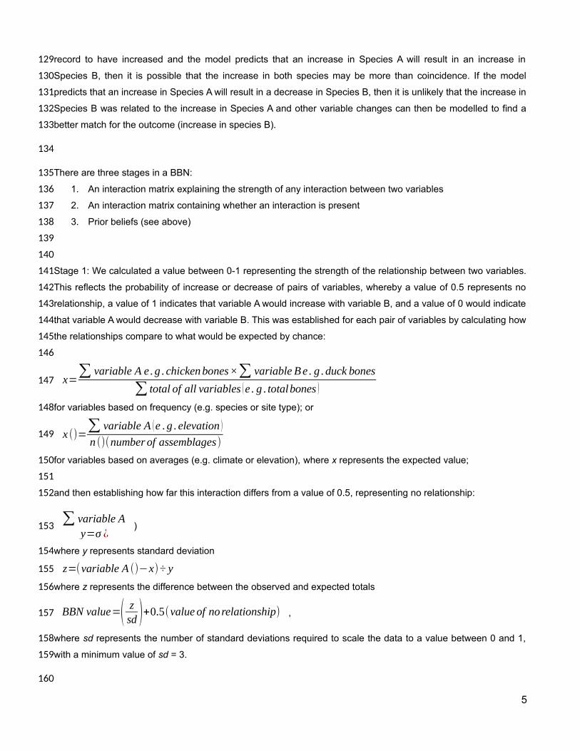
Stage 1: We calculated a value between 0-1 representing the strength of the relationship between two variables.
This reflects the probability of increase or decrease of pairs of variables, whereby a value of 0.5 represents no
relationship, a value of 1 indicates that variable A would increase with variable B, and a value of 0 would indicate
that variable A would decrease with variable B. This was established for each pair of variables by calculating how
the relationships compare to what would be expected by chance:
x=∑ variable A e .g . chickenbones×∑ variable Be . g .duck bones
∑ total of all variables (e . g . totalbones )
for variables based on frequency (e.g. species or site type); or
x ()=∑ variable A (e .g . elevation )
n ()(number of assemblages)
for variables based on averages (e.g. climate or elevation), where x represents the expected value;
and then establishing how far this interaction differs from a value of 0.5, representing no relationship:
∑ variable Ay=σ ¿
)
where y represents standard deviation
z=(variable A ()−x)÷ y
where z represents the difference between the observed and expected totals
BBN value=( zsd )+0.5(value of norelationship) ,
where sd represents the number of standard deviations required to scale the data to a value between 0 and 1,
with a minimum value of sd = 3.
5
129
130
131
132
133
134
135
136
137
138
139
140
141
142
143
144
145
146
147
148
149
150
151
152
153
154
155
156
157
158
159
160

Stage 2: If an interaction (positive or negative) was present, this was input into the second stage of the BBN.
Based on the formula above, relationships of 0.55 or above and 0.45 or below were interpreted as interactions.
As 0.5 represents no change, the range between 0.45 and 0.55 is unlikely to represent a meaningful
relationship.
Stage 3: We then adjusted the prior beliefs.. The model uses Bayesian inference to assess how changes, based
on observations from the archaeological record (e.g. an increase in chicken), would affect the other variables in
the study, based on their interactions with one another. Where a known increase or decrease occurred, albeit
limited by caveats associated with archaeological excavation (Pitt and Stewart in press), the prior belief was
adjusted to 1 or 0 respectively.
Species were selected based on association with chicken within specific spheres of interest (Table 1). The
chicken is found in the domestic sphere, along with the other primary domestic animals, dog, horse, pig,
sheep/goat, and the domestic birds, duck, goose and pigeon. Cattle were not selected for this analysis, as it has
been noted that comparison of cattle with other primary mammals and with birds is problematic, due to disposal
practices, recovery and preservation issues (Maltby 1997; Maltby 2010). It should be noted that duck, goose or
pigeons found on archaeological sites are not necessarily domestic but may have been merely tamed (Albarella
2005), or may represent other duck species (Parker 1988). Many of the selected domestic species are also
edible, as are partridge and quail, although partridge and quail are additionally of interest for their use as fighting
birds (Jennison 1937; Gal 2008).
Genera
Chicken Gallus
Dog Canis
Duck Anas, Aythya
Fox Vulpes
Goose Anser, Branta
Horse Equus
Marten Martes
Mouse Apodemus, Mus, Micromys
Partridge Alectoris, Perdix
Pig Sus
Pigeon Columba
Quail Coturnix
Rat Rattus
Sheep/goat Capra, Ovis
Sparrow Passer
Weasel/stoat Mustela
Table 1 Selected species.
3. Results and discussion 6
161
162
163
164
165
166
167
168
169
170
171
172
173
174
175
176
177
178
179
180
181
182
183

3.1 Analysis of changes in the faunal record
The known outcome from the archaeological data forms the prior beliefs and allows interpretation of the
Bayesian belief models. This study is concerned with understanding how known increases in chicken affected
other species with which it is associated, and whether changes in the frequency of those species may have
contributed to the increase in frequency of chicken found on archaeological sites. The data were analysed to
establish how species populations changed over time (Table 2).
Period 1 (to 800 BCE)
Period 2 (800 BCE - 0/42 CE)
Period 3 (1/43 - 500 CE)
NISP No. of sites NISP No. of sites NISP No. of sites
Total NISP
Total Sites
Chicken 16 2 4157 221 90040 468 94213 691
Dog 1087 23 21336 237 39903 356 62326 616
Duck 106 8 360 74 3415 197 3881 279
Fox 152 14 952 70 495 51 1599 135
Goose 44 6 308 59 4697 169 5049 234
Horse 542 17 42164 237 42881 398 85587 652
Marten 263 6 72 9 16 12 351 27
Mouse 0 0 215 16 906 44 1121 60
Partridge 20 4 39 12 598 32 657 48
Pig 7084 27 302716 275 216385 445 526185 747
Pigeon 3 2 515 26 799 104 1317 132
Quail 0 1 7 5 37 6 44 12
Rat 23 2 84 2 264 24 371 28
Sheep/goat 14524 27 341695 277 273019 446 629238 750
Sparrow 0 0 50 7 69 12 119 19
Weasel/stoat 6 3 46 18 209 29 261 50
Total 23870 28 714716 292 673733 504 1412319 824
Database Total (all mammals and birds)
105888
647 1002702
3242 1164718
7520 2273308 11409
Table 2. NISP and frequency of occurrence on sites
Domestic animals dominate the evidence in all periods, with bones of pig and sheep/goat recovered in greatest
frequency. Chicken is present in small numbers by period 2. By period 3 it is widespread with larger populations.
The change in frequency of chicken is paralleled by other species, including duck, goose, mouse, partridge,
quail, rat and weasel/stoat. Sparrow and pigeon also increase in frequency in period 3, but are present in
reasonable numbers in period 2. The increase in evidence of chicken in period 3 coincides with decreases in fox,
marten, pig and sheep/goat. The primary edible mammals experience minor population decreases in period 3,
but horse and dog continue to increase. Marten decrease over both periods.
3.2 Bayesian belief network analyses
7
184
185
186
187
188
189
190
191
192
193
194
195
196
197
198
199
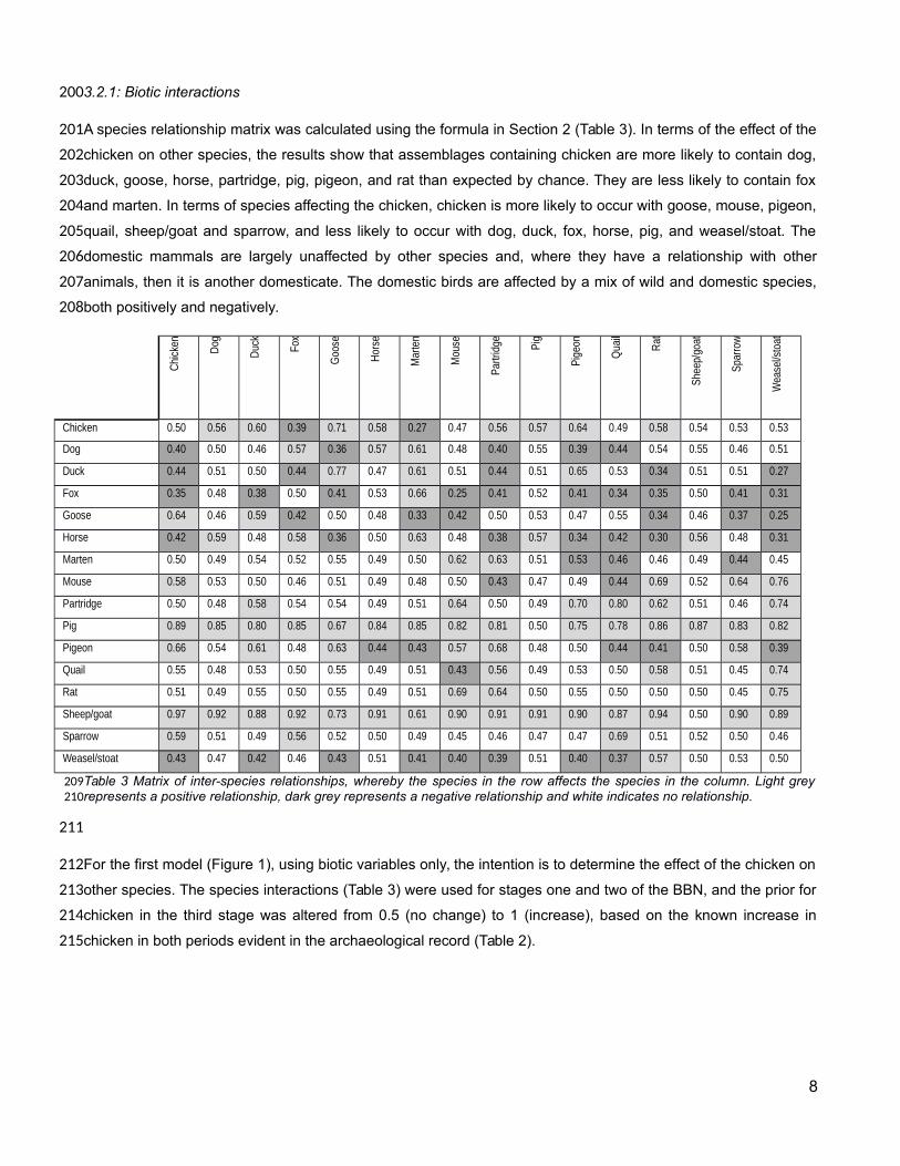
3.2.1: Biotic interactions
A species relationship matrix was calculated using the formula in Section 2 (Table 3). In terms of the effect of the
chicken on other species, the results show that assemblages containing chicken are more likely to contain dog,
duck, goose, horse, partridge, pig, pigeon, and rat than expected by chance. They are less likely to contain fox
and marten. In terms of species affecting the chicken, chicken is more likely to occur with goose, mouse, pigeon,
quail, sheep/goat and sparrow, and less likely to occur with dog, duck, fox, horse, pig, and weasel/stoat. The
domestic mammals are largely unaffected by other species and, where they have a relationship with other
animals, then it is another domesticate. The domestic birds are affected by a mix of wild and domestic species,
both positively and negatively.
Chick
en Dog
Duck Fox
Goo
se
Hors
e
Mar
ten
Mou
se
Partr
idge Pig
Pige
on
Qua
il
Rat
Shee
p/go
at
Spar
row
Wea
sel/s
toat
Chicken 0.50 0.56 0.60 0.39 0.71 0.58 0.27 0.47 0.56 0.57 0.64 0.49 0.58 0.54 0.53 0.53
Dog 0.40 0.50 0.46 0.57 0.36 0.57 0.61 0.48 0.40 0.55 0.39 0.44 0.54 0.55 0.46 0.51
Duck 0.44 0.51 0.50 0.44 0.77 0.47 0.61 0.51 0.44 0.51 0.65 0.53 0.34 0.51 0.51 0.27
Fox 0.35 0.48 0.38 0.50 0.41 0.53 0.66 0.25 0.41 0.52 0.41 0.34 0.35 0.50 0.41 0.31
Goose 0.64 0.46 0.59 0.42 0.50 0.48 0.33 0.42 0.50 0.53 0.47 0.55 0.34 0.46 0.37 0.25
Horse 0.42 0.59 0.48 0.58 0.36 0.50 0.63 0.48 0.38 0.57 0.34 0.42 0.30 0.56 0.48 0.31
Marten 0.50 0.49 0.54 0.52 0.55 0.49 0.50 0.62 0.63 0.51 0.53 0.46 0.46 0.49 0.44 0.45
Mouse 0.58 0.53 0.50 0.46 0.51 0.49 0.48 0.50 0.43 0.47 0.49 0.44 0.69 0.52 0.64 0.76
Partridge 0.50 0.48 0.58 0.54 0.54 0.49 0.51 0.64 0.50 0.49 0.70 0.80 0.62 0.51 0.46 0.74
Pig 0.89 0.85 0.80 0.85 0.67 0.84 0.85 0.82 0.81 0.50 0.75 0.78 0.86 0.87 0.83 0.82
Pigeon 0.66 0.54 0.61 0.48 0.63 0.44 0.43 0.57 0.68 0.48 0.50 0.44 0.41 0.50 0.58 0.39
Quail 0.55 0.48 0.53 0.50 0.55 0.49 0.51 0.43 0.56 0.49 0.53 0.50 0.58 0.51 0.45 0.74
Rat 0.51 0.49 0.55 0.50 0.55 0.49 0.51 0.69 0.64 0.50 0.55 0.50 0.50 0.50 0.45 0.75
Sheep/goat 0.97 0.92 0.88 0.92 0.73 0.91 0.61 0.90 0.91 0.91 0.90 0.87 0.94 0.50 0.90 0.89
Sparrow 0.59 0.51 0.49 0.56 0.52 0.50 0.49 0.45 0.46 0.47 0.47 0.69 0.51 0.52 0.50 0.46
Weasel/stoat 0.43 0.47 0.42 0.46 0.43 0.51 0.41 0.40 0.39 0.51 0.40 0.37 0.57 0.50 0.53 0.50
Table 3 Matrix of inter-species relationships, whereby the species in the row affects the species in the column. Light greyrepresents a positive relationship, dark grey represents a negative relationship and white indicates no relationship.
For the first model (Figure 1), using biotic variables only, the intention is to determine the effect of the chicken on
other species. The species interactions (Table 3) were used for stages one and two of the BBN, and the prior for
chicken in the third stage was altered from 0.5 (no change) to 1 (increase), based on the known increase in
chicken in both periods evident in the archaeological record (Table 2).
8
200
201
202
203
204
205
206
207
208
209210
211
212
213
214
215
Do
g
Du
ck
Fo
x
Go
ose
Ho
rse
Ma
rte
n
Mo
use
Pa
rtri
dg
e
Pig
Pig
eo
n
Qu
ail
Ra
t
Sh
ee
p/g
oa
t
Sp
arr
ow
We
ase
l
-60%
-40%
-20%
0%
20%
40%
60%
Affect on species predicted by increasing frequency of chickens
Pro
bab
ility
of
inc
rea
se
/de
cre
as
e
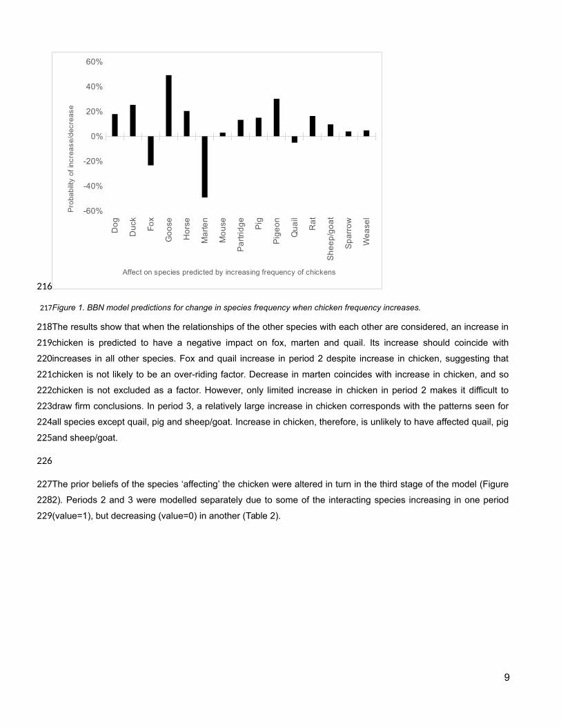
Figure 1. BBN model predictions for change in species frequency when chicken frequency increases.
The results show that when the relationships of the other species with each other are considered, an increase in
chicken is predicted to have a negative impact on fox, marten and quail. Its increase should coincide with
increases in all other species. Fox and quail increase in period 2 despite increase in chicken, suggesting that
chicken is not likely to be an over-riding factor. Decrease in marten coincides with increase in chicken, and so
chicken is not excluded as a factor. However, only limited increase in chicken in period 2 makes it difficult to
draw firm conclusions. In period 3, a relatively large increase in chicken corresponds with the patterns seen for
all species except quail, pig and sheep/goat. Increase in chicken, therefore, is unlikely to have affected quail, pig
and sheep/goat.
The prior beliefs of the species ‘affecting’ the chicken were altered in turn in the third stage of the model (Figure
2). Periods 2 and 3 were modelled separately due to some of the interacting species increasing in one period
(value=1), but decreasing (value=0) in another (Table 2).
9
216
217
218
219
220
221
222
223
224
225
226
227
228
229
Incr
ea
se d
og
Incr
ea
se d
uck
Incr
ea
se fo
x
De
cre
ase
fox
Incr
ea
se g
oo
se
Incr
ea
se h
ors
e
Incr
ea
se m
ou
se
Incr
ea
se p
ig
De
cre
ase
pig
Incr
ea
se p
ige
on
Incr
ea
se q
ua
il
Incr
ea
se s
he
ep
/go
at
De
cre
ase
sh
ee
p/g
oa
t
Incr
ea
se s
pa
rro
w
Incr
ea
se w
ea
sel
-100%
-80%
-60%
-40%
-20%
0%
20%
40%
60%
80%
100%
Period 2 Period 3
Species affecting chicken
Pro
bab
ility
of
inc
rea
se/d
ec
rea
se
of c
hic
ke
n
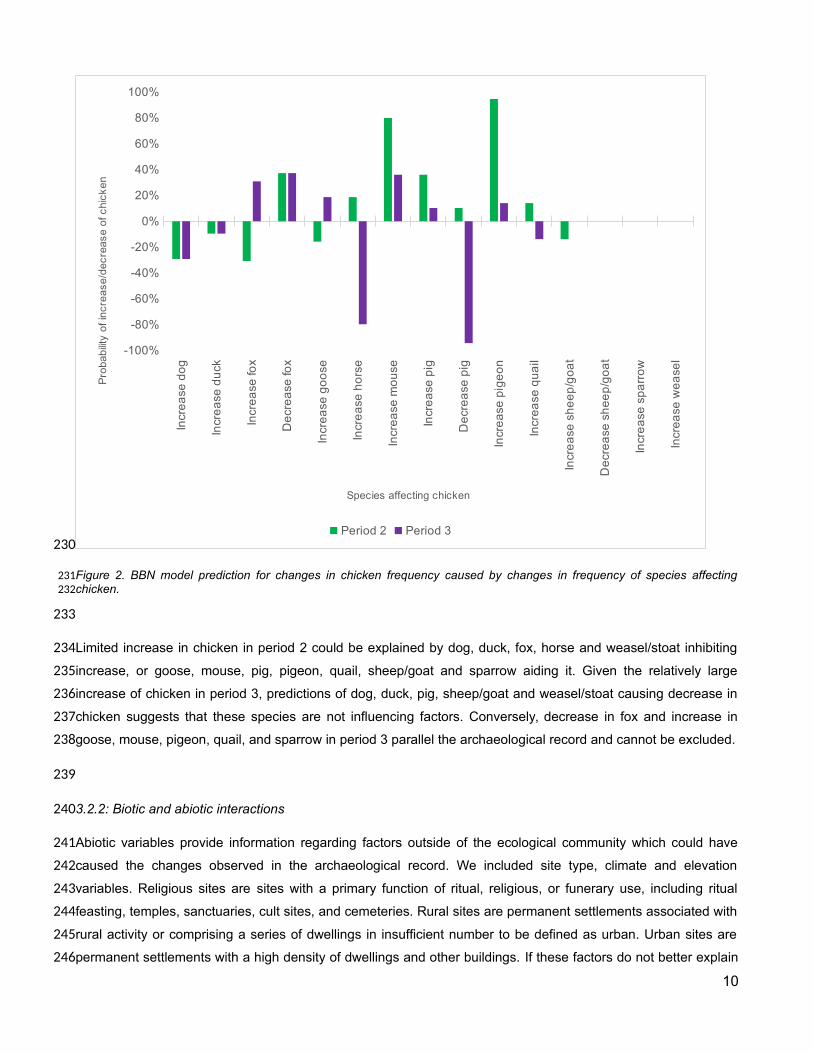
Figure 2. BBN model prediction for changes in chicken frequency caused by changes in frequency of species affectingchicken.
Limited increase in chicken in period 2 could be explained by dog, duck, fox, horse and weasel/stoat inhibiting
increase, or goose, mouse, pig, pigeon, quail, sheep/goat and sparrow aiding it. Given the relatively large
increase of chicken in period 3, predictions of dog, duck, pig, sheep/goat and weasel/stoat causing decrease in
chicken suggests that these species are not influencing factors. Conversely, decrease in fox and increase in
goose, mouse, pigeon, quail, and sparrow in period 3 parallel the archaeological record and cannot be excluded.
3.2.2: Biotic and abiotic interactions
Abiotic variables provide information regarding factors outside of the ecological community which could have
caused the changes observed in the archaeological record. We included site type, climate and elevation
variables. Religious sites are sites with a primary function of ritual, religious, or funerary use, including ritual
feasting, temples, sanctuaries, cult sites, and cemeteries. Rural sites are permanent settlements associated with
rural activity or comprising a series of dwellings in insufficient number to be defined as urban. Urban sites are
permanent settlements with a high density of dwellings and other buildings. If these factors do not better explain
10
230
231232
233
234
235
236
237
238
239
240
241
242
243
244
245
246

the observed changes, then they are unlikely to be major driving factors. The relationships between the abiotic
variables and both the chicken and the species affected by chicken (Table 4), were calculated as per the method
in Section 2.
Chick
en Dog
Duck Fox
Goo
se
Hors
e
Mar
ten
Partr
idge Pig
Pige
on Rat
Religious 0.65 0.45 0.5 0.43 0.5 0.5 0.5 0.5 0.5 0.58 0.61Rural 0.5 0.56 0.5 0.63 0.5 0.5 0.65 0.5 0.5 0.45 0.86
Urban 0.39 0.5 0.55 0.44 0.5 0.5 0.39 0.55 0.5 0.5 0.03
Elevation 0.46 0.40 0.27 0.47 0.29 0.41 0.83 0.91 0.43 0.58 0.61
Temperature 0.5 0.43 0.38 0.5 0.4 0.42 0.5 0.94 0.5 0.5 0.62
Precipitation 0.4 0.38 0.43 0.21 0.3 0.39 0.43 0.94 0.43 0.76 0.68
Table 4. Matrix of species relationships with climate and environment variables, whereby the variable in the row affects the
species in the column. Light grey represents a positive relationship, dark grey represents a negative relationship and white
indicates no relationship.
The abiotic variable relationships were added to stages one and two of the model. The inter-species
relationships were retained. The prior beliefs of each of the abiotic variables were altered in the third stage of the
model to reflect known changes (Figure 3), as observed in historical records (climate) or derived from the
dataset (elevation at site locations and site type). Known changes in period 2, compared to period 1, include a
decrease in religious sites; and increase in rural and urban sites. The average height of a site above sea level
increases, as does annual rainfall. In period 3, urban sites increase at the expense of rural sites; sites are
located at lower elevation, and annual rainfall decreases slightly, compared to period 2.
11
247
248
249
250
251252
253
254
255
256
257
258
259
260
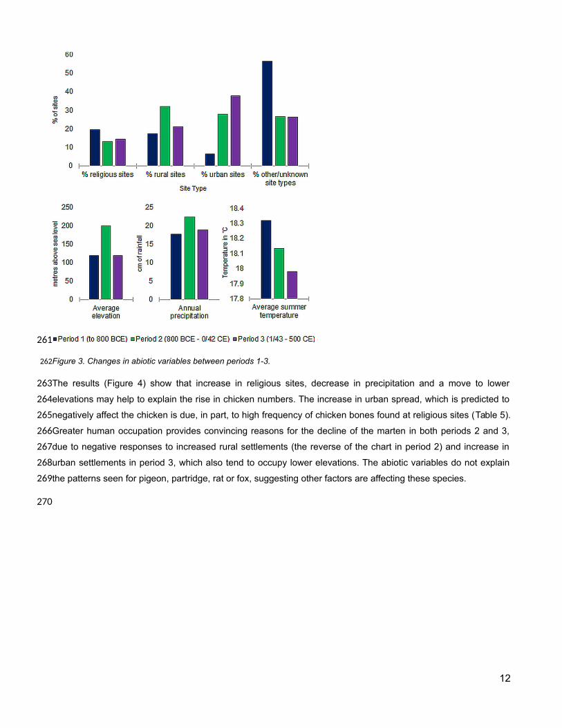
Figure 3. Changes in abiotic variables between periods 1-3.
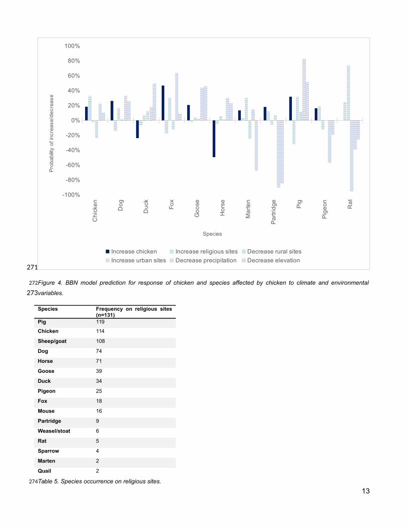
The results (Figure 4) show that increase in religious sites, decrease in precipitation and a move to lower
elevations may help to explain the rise in chicken numbers. The increase in urban spread, which is predicted to
negatively affect the chicken is due, in part, to high frequency of chicken bones found at religious sites (Table 5).
Greater human occupation provides convincing reasons for the decline of the marten in both periods 2 and 3,
due to negative responses to increased rural settlements (the reverse of the chart in period 2) and increase in
urban settlements in period 3, which also tend to occupy lower elevations. The abiotic variables do not explain
the patterns seen for pigeon, partridge, rat or fox, suggesting other factors are affecting these species.
12
261
262
263
264
265
266
267
268
269
270
Ch
icke
n
Do
g
Du
ck
Fo
x
Go
ose
Ho
rse
Ma
rte
n
Pa
rtri
dg
e
Pig
Pig
eo
n
Ra
t
-100%
-80%
-60%
-40%
-20%
0%
20%
40%
60%
80%
100%
Increase chicken Increase religious sites Decrease rural sites
Increase urban sites Decrease precipitation Decrease elevation
Species
Pro
bab
ility
of
inc
rea
se/d
ec
rea
se
Figure 4. BBN model prediction for response of chicken and species affected by chicken to climate and environmental
variables.
Species Frequency on religious sites(n=131)
Pig 119
Chicken 114
Sheep/goat 108
Dog 74
Horse 71
Goose 39
Duck 34
Pigeon 25
Fox 18
Mouse 16
Partridge 9
Weasel/stoat 6
Rat 5
Sparrow 4
Marten 2
Quail 2
Table 5. Species occurrence on religious sites.
13
271
272
273
274

3.2.3 Recovery methods
One of the main benefits of this kind of model is that it is not limited to purely environmental variables. This
allows testing of a further theory- that the frequency of small animals is affected by excavation recovery
methods. Larger bones are easier to detect during hand excavation, and smaller ones more likely to be missed
unless contexts are sieved (Payne 1972; Sapir-Hen et al. 2017). Other factors influence whether sieving is part
of the excavation methodology, and these were included in the models. Type of site was included because
religious sites, particularly burials and cremations, are more likely to be sieved. This was confirmed by the
relationship calculation (Table 6 and 7), after the method presented in Section 2. The type of excavation, whether
commercial, rescue or research can influence the type of site excavated and whether sieving is performed. Bone
condition also affects whether more bones are recovered by sieving, and sieving was calculated to procure
greater numbers of bones in poor condition.
Chick
en Dog
Duck Fox
Goo
se
Hors
e
Mar
ten
Mou
se
Partr
idge Pi
g
Pige
on
Qua
il
Rat
Shee
p/go
at
Spar
row
Wea
sel/s
toat
Hand excavated 0.33 0.5 0.5 0.3 0.5 0.5 0.5 0.01 0.52 0.54 0 0.39 0.29 0.31 0.51 0.43
Sieved 0.67 0.5 0.5 0.7 0.5 0.5 0.5 0.99 0.48 0.46 1 0.61 0.71 0.69 0.49 0.57
Good condition 0.34 0.5 0.5 0.4 0.5 0.5 0.36 0.32 0.54 0.51 0.02 0.55 0.42 0.51 0.52 0.55
Poor condition 0.68 0.5 0.5 0.43 0.56 0.5 0.64 0.69 0.46 0.5 0.58 0.47 0.43 0.48 0.5 0.46
Commercial 0.45 0.88 1 0.58 0.69 0.51 0.44 0.48 0.45 0.47 0.44 0.42 0.71 0.52 0.48 0.46
Rescue 0.67 0.43 0 0.49 0.5 0.44 0.79 0.3 0.27 0.36 0.32 0.3 0.18 0.64 0.8 0.27
Research 0.38 0.19 0 0.43 0.31 0.55 0.27 0.72 0.78 0.67 0.74 0.78 0.61 0.34 0.23 0.77
Religious 0.7 0.43 0.5 0.4 0.5 0.5 0.5 0.5 0.45 0.47 0.58 0.44 0.62 0.49 0.48 0.45
Rural 0.44 0.56 0.5 0.61 0.44 0.5 0.69 0.5 0.47 0.49 0.39 0.46 0.8 0.52 0.7 0.7
Urban 0.38 0.5 0.57 0.43 0.5 0.5 0.37 0.28 0.58 0.55 0.39 0.56 0.03 0.48 0.34 0.34
Table 6. Matrix of species and recovery method variables relationships, whereby the variable in the row affects the species inthe column. Light grey represents a positive relationship, dark grey represents a negative relationship and white indicates norelationship.
Hand
exc
avat
ed
Siev
ed
Poor
con
ditio
n
Relig
ious
Rura
l
Urba
n
Hand excavated 0.5 0.5 0.5 0.38 0.5 0.5Sieved
0.5 0.5 0.5 0.62 0.5 0.5Good condition
0.5 0.5 0.5 0.5 0.5 0.5Poor condition
0.5 0.5 0.5 0.5 0.5 0.5Commercial
0.5 0.5 0.5 0.5 0.5 0.5Rescue
0.5 0.5 0.5 0.5 0.5 0.5
14
275
276
277
278
279
280
281
282
283
284
285
286
287288289
290

Research 0.76 0 0.5 0.5 0.5 0.5
Religious 0.43 0.73 0.5 0.5 0.5 0.5
Rural0.5 0.44 0.5 0.5 0.5 0.5
Urban 0.55 0.33 0.5 0.5 0.5 0.5
Table 7. Matrix of recovery method variables relationships, whereby the variable in the row affects the variable in the column.Light grey represents a positive relationship, dark grey represents a negative relationship and white indicates no relationship.
These relationships were used in stages one and two of the BBN to assess the predicted increase in NISP if
more sieving is done (value=1 in stage three) (Figure 5). Inter-species relationships were not included as they
are not relevant to this analysis. The model predicts that nine of the species in this study are likely to benefit from
more sieving, especially mouse and pigeon. Sieving would not decrease recovery of any of these species.
Ch
icke
n
Do
g
Du
ck
Fo
x
Go
ose
Ho
rse
Ma
rte
n
Mo
use
Pa
rtri
dg
e
Pig
Pig
eo
n
Qu
ail
Ra
t
Sh
ee
p/g
oa
t
Sp
arr
ow
We
ase
l
0%
10%
20%
30%
40%
50%
60%
70%
80%
90%
100%
Species
Pro
bab
ility
of
inc
rea
se w
ith m
ore
sie
vin
g
Figure 5. BBN model prediction for recovery of animal bones with more sieving.
4. Discussion: Analysis of presence on archaeological sites shows that increase in chicken occurs at the same
time as changes in other species related to the chicken in various spheres of influence. Decreases in pig and
sheep/goat and only minimal increase in horse in period 3 suggests that observed increase of other species is
not merely because of population size increases. The largest percentage change observed is the chicken in
period 3. This large increase of chicken also coincides with increases in duck, goose, mouse, partridge, quail, rat
and weasel/stoat and decreases in fox and marten. As a predator species, which is known to steal eggs, the
15
291292
293
294
295
296
297
298
299
300
301
302
303
304
305
306

fortune of the weasel/stoat contrasts with that of the fox and marten. This raises interesting observations for
further analysis. Does the chicken affect the increase of weasel/stoat and cause fox and marten to decline?
Perhaps the weasel/stoat is perceived differently by humans (after O'Connor 2013a)? Does the presence of
other domestic species cause higher occurrence of chicken, and vice versa? Or does the increasing popularity of
the chicken in period 3 cause proportional decreases in the primary domesticates? Does the method of feeding
chickens enhance populations of commensal species such as mouse, rat, feral pigeon and sparrow? Are other
factors causing these changes instead?
Calculating the relationships for the Bayesian belief network inter-species model identified that the ecosystem
dynamics are different for domestic birds compared to domestic mammals, and, given the wide range of species
that affect or are affected by chicken, the chicken belongs in a domestic sphere influenced by the other domestic
birds. The models predicted that chicken neither influenced, nor was influenced by, the primary domestic
mammals. Changing dietary patterns between periods 2 and 3 (King 1999) and particularly the varied diet
enjoyed by the Romans (Rowan 2017), at least on some sites, might offer a good explanation for the increase in
birds, and slight decrease in domestic mammals. The models predict that goose and pigeon are most likely to
increase chicken. This may be due to their position within the domestic sphere. Goose husbandry is well
established by the Roman period, but duck domestication appears to be in its infancy, based on ancient literature
(Albarella 2005). Positive association of duck with urban settlements and lower elevations may, therefore, be
explained by importation into towns (after Parker 1988). Association with religious sites, consistent with the
findings of King (2005), is predicted to be the abiotic variable most affecting chicken.
Chickens are, however, known to be frequently found in towns (Maltby 1997). As common quail prefer open,
agricultural habitats (BirdLife International 2016), it might be expected that they should not be found associated
with chicken. Yet, an increase in quail is predicted to increase chicken populations. An increase in chicken,
however, is predicted to reduce numbers of quail. The known evidence suggests otherwise. They are both
fighting, edible birds and quail could be imported to towns for these purposes. The same is true for partridge, the
other fighting bird, which is predicted to increase with increased numbers of chicken. Environmental variables
cannot explain what is seen in the faunal record. This suggests that the increase of the chicken is not to the
detriment of the other potential fighting birds.
Environmental variables, particularly the spread of urbanisation, deforestation, and construction of settlements at
lower elevations explain the reduction of marten in the archaeological record better than the influence of chicken,
although exacerbation by increase of chicken in period 3 is not discounted. The models show that the effect of
the chicken on the other egg-thief, weasel/stoat is little more than expected by chance, and that the weasel/stoat
does not, in fact, affect chicken. Of the predators, fox matches the pattern seen in the archaeological data, with
16
307
308
309
310
311
312
313
314
315
316
317
318
319
320
321
322
323
324
325
326
327
328
329
330
331
332
333
334
335
336
337
338
339
340
341
its increase perhaps inhibiting numbers of chicken initially and then experiencing population decline as chicken
appears more frequently in the archaeological record.
The other small birds, sparrow and pigeon, along with mouse and rat, are predicted to increase with increased
numbers of chicken, and thus the introduction of the chicken may have benefited these species. These species
are all small and recovery is likely to have been a major issue. Mouse, pigeon and rat were all shown to benefit
from more sieving. This suggests that the frequency of small mammals and birds present was, in all likelihood,
higher, but that they were not recovered. With the exception, perhaps, of pigeon, they are all also species which
have less direct human interaction and so their presence on archaeological sites is opportunistic. Their remains
are more likely to be found where humans have chosen to deposit their refuse, rather than in the main centres of
human activity (O'Connor 2013b) and so are likely to be underrepresented in the archaeological literature.
There is another explanation, not accounted for in the models, which could apply to rat and to fox. These two
species are a problem for chicken keepers because foxes can decimate a flock, while rats can contaminate feed
and water and cause disease in humans (Graham 2015). Both animals would thrive around chickens, and eat
their eggs, were it not for humans, who will take measures to protect their flock from them. This offers a good
explanation for the predicted and observed results for fox, which increases in period 2 while chicken is present,
but only in low frequency and has been newly introduced. It decreases in period 3 when chicken increases
dramatically and humans are likely to have developed better means of protecting them. This is consistent with a
study of Anglo-Saxon fauna, which identified no direct correlation between chicken and fox (Poole 2015). Poole
(2015) suggested that, in these instances, humans may have been reducing the fox population as a threat to
human infant burials.
5. Conclusions: The impact of the chicken on its environment and of the environment on the chicken was
examined using a novel method to identify and exclude potential causes and effects. Analysis of the
relationships and associations between species found in similar spheres of human activity, and their responses
to external environmental factors, allows us to establish which of the many possible correlations are likely to
have contributed to, or been most affected by, the success of the chicken in Europe. The results show that
chicken demonstrate most affinity with the other domestic birds. Where chicken is found, goose and pigeon are
more likely to be found, and, indirectly, duck via a positive mutual relationship between duck and goose. Its
introduction and success did not affect the primary domestic mammals, nor the other fighting birds, quail and
partridge, possibly due to their use as food also.
The introduction of the chicken was shown to most affect fox, partridge and pigeon. Increase in chicken, directly
or indirectly, provides the best explanation for the decrease of fox, having established that environmental
17
342
343
344
345
346
347
348
349
350
351
352
353
354
355
356
357
358
359
360
361
362
363
364
365
366
367
368
369
370
371
372
373
374
375
376

changes in period 3 should have led to increases in fox numbers. While the chicken may have contributed to the
decline of marten, external environmental factors, particularly the spread of urbanisation, offer a better
explanation. Increase in chicken may have aided increases in mouse, quail and rat; although models suggest
that recovery of these species, which are present in low numbers in the dataset, are affected by retrieval
methods and may be under-represented. Recovery models find that sieving would enhance recovery of nine of
the sixteen species assessed (over 50%), making it a worthy endeavour for small animal assemblages.
The results are model predictions and must be interpreted as such. In this study, interpretation is restricted to
better understanding of the information present in the data. For future work, if two independent datasets were
available, this would enable the user to establish the prior beliefs from one dataset, and use this information to
test hypotheses from another dataset. This would facilitate testing of site scale hypotheses as well as those at
larger regional scales. Local or regional study of detailed recovery techniques may also provide interesting
results. This study presents a method which can be easily applied to any archaeological dataset. It demonstrates
how an inter-disciplinary approach, using novel ecological techniques, offers an efficient means of comparing
various inter-related aspects of large quantities of data and can help to better interpret the archaeological record.
Acknowledgments: This research was funded by Bournemouth University, in association with the AHRC (Grant
No AH/L006979/1). We would like to thank the two anonymous reviewers who helped to improve this study.
18
377
378
379
380
381
382
383
384
385
386
387
388
389
390
391
392
393
394

References:
Albarella, U., 2005. Alternate fortunes? The role of domestic ducks and geese from Roman to Medieval times in Britain. In: Grupe, G. and Peters, J., eds. Feathers, grit and symbolism: Birds and humans in the ancient Old and New Worlds. Proceedings of the 5th Meeting of the ICAZ Bird WorkingGroup in Munich [26.7.-28.7.2004]. Rahden: Verlag Marie Leidorf, 249-258.
Araújo, M. B. and Rozenfeld, A., 2014. The geographic scaling of biotic interactions. Ecography, 37 (5), 406-415.
Baselga, A. and Araújo, M. B., 2009. Individualistic vs community modelling of species distributions under climate change. Ecography, 32 (1), 55-65.
BirdLife International, 2016. Coturnix coturnix. The IUCN Red List of threatened species 2016: e.T22678944A85846515. [online]. Available from: http://dx.doi.org/10.2305/IUCN.UK.2016-3.RLTS.T22678944A85846515.en [Accessed 1 February 2017].
Boev, Z., 1993. Archeo-ornithology and the synanthropisation of birds: A case study for Bulgaria. Archaeofauna: Revista de la Asociación Española de Arqueozoología, 2, 145-153.
Büntgen, U., Tegel, W., Nicolussi, K., McCormick, M., Frank, D., Trouet, V., Kaplan, J. O., Herzig, F., Heussner, K.-U., Wanner, H., Luterbacher, J. and Esper, J., 2011. 2500 years of European climate variability and human susceptibility. Science, 331, (6017), 578-582.
CGIAR Consortium for Spatial Information, 2008. Resampled SRTM data to 250m resolution (based on SRTM 90m Digital Elevation Model) [online]. Available from: http://srtm.csi.cgiar.org/ [Accessed 16 December 2015].
Davis, S. J. M., 2012. The archaeology of animals. London: Routledge.
Elevelt, S. C., 2012. Subsistence and social stratification in Northern Ionic Calabria from the Middle Bronze Age until the Early Iron Age: the archaeozoological evidence. Thesis (Doctor of Philosophy). Groningen.
Gal, E., 2008. Bone evidence of pathological lesions in domestic hen (Gallus domesticus Linnaeus, 1758). Veterinarija ir Zootechnika, 41 (63), 42-48.
Graham, C., 2015. The chicken keeper's problem solver. 100 common problems explored andexplained. London: Hamlyn.
Hijmans, R. J., Cameron, S. E., Parra, J. L., Jones, P. G. and Jarvis, A., 2005. Very high resolution interpolated climate surfaces for global land areas. International Journal of Climatology, 25 (15), 1965-1978.
Jennison, G., 1937. Animals for Show and Pleasure in Ancient Rome. Manchester University Press.
King, A., 1999. Diet in the Roman world: a regional inter-site comparison of the animal bones. Journal of Roman Studies, 12, 168-202.
King, A., 2005. Animal remains from temples in Roman Britain. Britannia, 36, 329-369
Kissling, W. D., Dormann, C. F., Groeneveld, J., Hickler, T., Kühn, I., McInerny, G. J., Montoya, J. M., Römermann, C., Schiffers, K., Schurr, F. M., Singer, A., Svenning, J.-C., Zimmermann, N. E. and O’Hara, R. B., 2012. Towards novel approaches to modelling biotic interactions in multispecies assemblages at large spatial extents. Journal of Biogeography, 39 (12), 2163-2178.
Lang, J. M. and Benbow, M. E., 2013. Species interactions and competition. Nature Education Knowledge, 4 (4), 8.
19
395
396397398399
400401
402403
404405406
407408
409410411
412413414
415
416417418
419420
421422423424425426
427
428429
430
431432433434
435436
Maltby, M., 1997. Domestic fowl on Romano‐British sites: inter‐site comparisons of abundance. International Journal of Osteoarchaeology, 7 (4), 402-414.
Maltby, M., 2010. Feeding a Roman town: environmental evidence from excavations in Winchester,1972-1985. Winchester: Winchester Museums.
Mauri, A., Davis, B. A. S., Collins, P. M. and Kaplan, J. O., 2015. The climate of Europe during the Holocene: a gridded pollen-based reconstruction and its multi-proxy evaluation. Quaternary Science Reviews, 112, 109-127.
McInerny, G. J. and Purves, D. W., 2011. Fine-scale environmental variation in species distribution modelling: regression dilution, latent variables and neighbourly advice. Methods in Ecology and Evolution, 2 (3), 248-257.
Mooney, H. A. and Cleland, E. E., 2001. The evolutionary impact of invasive species. Proceedings of the National Academy of Sciences, 98 (10), 5446-5451.
O'Connor, T. P., 1993. Birds and the scavenger niche. Archaeofauna: Revista de la Asociación Española de Arqueozoología, 2, 155-162.
O'Connor, T., 2013a. Animals as neighbors: The past and present of commensal animals. East Lansing: Michigan State University Press.
O'Connor, T., 2013b. The archaeology of animal bones. New York: The History Press.
Parker, A. J., 1988. The birds of Roman Britain. Oxford Journal of Archaeology, 7 (2), 197-226.
Parmentier, E. and Michel, L., 2013. Boundary lines in symbiosis forms. Symbiosis, 60 (1), 1-5.
Payne, S., 1972. Partial recovery and sample bias: The results of some sieving experiments. In: Higgs, E. S., ed. Papers in Economic Prehistory. London: Cambridge University Press, 49-64.
Pearson, R. G. and Dawson, T. P., 2003. Predicting the impacts of climate change on the distribution of species: are bioclimate envelope models useful? Global Ecology and Biogeography, 12 (5), 361-371.
Pitt, J., 2017. The ecology of chickens: An examination of the introduction of the domestic chickenacross Europe after the Bronze Age. Thesis (Doctor of Philosophy). Bournemouth University.
Pitt, J., Gillingham, P. K., Maltby, M. and Stewart, J. R., 2016. New perspectives on the ecology of early domestic fowl: An interdisciplinary approach. Journal of Archaeological Science, 74, 1-10.
Pitt, J. and Stewart, J. R., in press. Garbage in, garbage out? Issues and suggestions for small vertebrate zooarchaeological databases. Submitted to British Archaeological Reports.
Pollock, L. J., Tingley, R., Morris, W. K., Golding, N., O'Hara, R. B., Parris, K. M., Vesk, P. A. and McCarthy, M. A., 2014. Understanding co-occurrence by modelling species simultaneously with a JointSpecies Distribution Model (JSDM). Methods in Ecology and Evolution, 5 (5), 397-406.
Poole, K., 2015. Foxes and badgers in Anglo-Saxon life and landscape. Archaeological Journal, 172 (2), 389-422.
Rowan, E., 2017. Sewers, archaeobotany, and diet at Pompeii and Herculaneum. In: Flohr, M. and Wilson, A., eds. The economy of Pompeii. Oxford: Oxford University Press, 111-134.
Sapir-Hen, L., Sharon, I., Gilboa, A. and Dayan, T., 2017. Wet sieving a complex tell: Implications for retrieval protocols and studies of animal economy in historical periods. Journal of Archaeological Science, 82, 72-79.
20
437438
439440
441442443
444445446
447448
449450
451452
453
454
455
456457
458459460
461462
463464
465466
467468469
470471
472473
474475476

Soberón, J. and Nakamura, M., 2009. Niches and distributional areas: Concepts, methods, and assumptions. Proceedings of the National Academy of Sciences, 106 (Supplement 2), 19644-19650.
Spiers, E. K. A., Stafford, R., Ramirez, M., Vera Izurieta, D. F., Cornejo, M. and Chavarria, J., 2016. Potential role of predators on carbon dynamics of marine ecosystems as assessed by a Bayesian belief network. Ecological Informatics, 36, 77-83.
Stafford, R., Williams, R. L. and Herbert, R. J. H., 2015. Simple, policy friendly, ecological interaction models from uncertain data and expert opinion. Ocean & Coastal Management, 118, Part A, 88-96.
Stewart, J. R., 2009. The evolutionary consequence of the individualistic response to climate change. Journal of Evolutionary Biology, 22 (12), 2363-2375.
Wilkinson, P., 2007. Archaeology : what it is, where it is, and how to do it. Oxford: Archaeopress.
Wisz, M. S., Pottier, J., Kissling, W. D., Pellissier, L., Lenoir, J., Damgaard, C. F., Dormann, C. F., Forchhammer, M. C., Grytnes, J.-A., Guisan, A., Heikkinen, R. K., Høye, T. T., Kühn, I., Luoto, M., Maiorano, L., Nilsson, M.-C., Normand, S., Öckinger, E., Schmidt, N. M., Termansen, M., Timmermann, A., Wardle, D. A., Aastrup, P. and Svenning, J.-C., 2013. The role of biotic interactions inshaping distributions and realised assemblages of species: implications for species distribution modelling. Biological Reviews, 88 (1), 15-30.
Zeiler, J. T. and de Vries, L. S., 2008. Archeozoölogisch onderzoek van de Romeinse stad Forum Hadriani (120-270 AD), gem. Leidschendam-Voorburg (LVB-FO 9888). Leeuwarden: ArchaeoBone.
21
477478
479480481
482483
484485
486
487488489490491492
493494
495
496


