
1
Channel Tracking using Particle Filtering in
unresolvable Multipath Environments
Tanya Bertozzi†*, Didier Le Ruyet*, Cristiano Panazio* and Han Vu-Thien *
† DIGINEXT, 45 impasse de la Draille, 13857 Aix en Provence Cedex 3, France,
Tel.: 0033 4 42 90 82 82, Fax: 0033 4 42 90 82 80, Email: [email protected]
* CNAM, 292 rue Saint Martin, 75141 Paris Cedex 3, France
Tel.: 0033 1 58 80 84 91, Email: [email protected]
December 24, 2003 DRAFT

2
Abstract
In this paper we propose a new timing error detector for timing tracking loops inside the Rake
receiver in spread spectrum systems. Based on a particle filter, this timing error detector jointly tracks
the delays of each path of the frequency selective channels. Instead of using conventional channel
estimator we have introduced a joint time delay and channel estimator without almost no additional
computational complexity. The proposed scheme avoids the drawback of the classical early late gate
detector which is not able to separate closely spaced paths. Simulation results show that the proposed
detectors outperform the conventional early late gate detector in indoor scenarios.
Index Terms
Sequential Monte Carlo, multipath channels, importance sampling, timing estimation.
I. INTRODUCTION
In wireless communications, Direct-Sequence Spread Spectrum (DS-SS) techniques have re-
ceived an increasing interest, especially for the third generation of mobile systems. In DS-SS
systems, the adapted filter typically employed is the Rake receiver. This receiver is efficient to
counteract the effects of frequency-selective channels. It is composed of fingers, each assigned to
one of the most significant channel paths. The outputs of the fingers are combined proportionally
to the power of each path for estimating the transmitted symbols (maximum ratio combining).
Unfortunately, the performance of the Rake receiver strongly depends on the quality of the
estimation of the parameters associated with the channel paths. As a consequence, we have to
estimate the delay of each path using a Timing Error Detector (TED). This goal is generally
achieved in two steps: acquisition and tracking. During the acquisition phase, the number and the
delays of the most significant paths are determined. These delays are estimated within one half
chip from the exact delays. Then, the tracking module refines the first estimation and follows
the delay variations during the permanent phase. The conventional TED used during the tracking
phase is the Early Late Gate-TED (ELG-TED) associated with each path. It is well known that
the ELG-TED works very well in the case of a single fading path. However, in the presence of
multipath propagation, the interference between the different paths can degrade its performance.
In fact, the ELG-TED cannot separate the individual paths when they are closer than one chip
period from the other paths, whereas a discrimination up to Tc/4 can still increase the diversity
December 24, 2003 DRAFT
3
of the receiver (Tc denotes the chip time) [1]. When the difference between the delays of two
paths is contained in the interval 0-1.5 Tc, we are in the presence of unresolvable multipaths.
This scenario corresponds for example to the indoor scenario. The problem of unresolvable
multipaths has been recently analyzed in [2] [3] [4].
Particle filtering (PF) or Sequential Monte Carlo (SMC) methods [5] represent the most
powerful approach for the sequential estimation of the hidden state of a nonlinear dynamic
model. The solution to this problem depends on the knowledge of the Posterior Probability
Density (PPD) of the hidden state given the observations. Except in a few special cases including
linear Gaussian system models, it is impossible to calculate analytically a sequential expression
of this PPD. It is necessary to adopt numerical approximations. The PF methods give a discrete
approximation of the PPD of the hidden state by weighted points or particles which can be
recursively updated as new observations become available.
The first main application of the PF methods was target tracking. More recently, these tech-
niques have been successfully applied in communications, including blind equalization in Gaus-
sian [6] and non-Gaussian [7], [8] noises and joint symbol and timing estimation [9]. For a
complete survey of the communication problems dealt with using PF methods, see [10].
In this paper we propose to use the PF methods for estimating the delays of the paths in
multipath fading channels. Since these methods are based on a joint approach, they provide
optimal estimates of the different channel delays. In this way, we can overcome the problem of
the adjacent paths which causes the failure of the conventional single path tracking approaches
in the presence of unresolvable multipaths. Moreover, we will combine the PF-based TED (PF-
TED) with a conventional estimator for estimating the amplitudes of the channel coefficients. We
will also apply the PF methods to the estimation of the channel coefficients in order to jointly
estimate the delays and the coefficients.
This paper is organized as follows. In Section 2, we will introduce the system model. Then
in Section 3, we will describe the conventional ELG-TED and the PF-TED. In Section 4, we
will present the conventional estimators of the channel coefficients and the application of the PF
methods to the joint estimation of the delays and the channel coefficients. In Section 5, we will
give simulation results. Finally, we will draw a conclusion in Section 5.
December 24, 2003 DRAFT

4
II. SYSTEM MODEL
We consider a DS-SS system sending a complex data sequence {sn} . The data symbols are
spread by a spreading sequence {dm}Ns−1m=0 where Ns is the spreading factor.
The resulting baseband equivalent transmitted signal is given by:
e(t) =∑
n
sn
Ns−1∑
m=0
dmg(t − mTc − nT ), (1)
where Tc and T are respectively the chip and symbol period and g(t) is the impulse response
of the root-raised cosine filter with a rolloff factor equal to 0.22 in the case of the Universal
Mobile Telecommunications System (UMTS) [11].
h(t, τ) denotes the overall impulse response of the multipath propagation channel with Lh
independent paths (Wide Sense Stationary Uncorrelated Scatterers (WSSUS) model):
h(t, τ) =
Lh∑
l=1
hl(t)δ(τ − τl(t)). (2)
Each path is characterized by its time-varying delay τl(t) and channel coefficient hl(t).
The signal at the output of the matched filter is given by:
r(t) =
Lh∑
l=1
hl(t)∑
n
sn
Ns−1∑
m=0
dmRg(t − mTc − nT − τl(t)) + n(t), (3)
where n(t) represents the Additive White Gaussian Noise (AWGN) n(t) filtered by the matched
filter and
Rg(t) =
∫ +∞
−∞
g∗(τ)g(t + τ)dτ (4)
is the total impulse response of the transmission and receiver filters.
Fig. 1 shows the equivalent lowpass transmission model considered in this paper.
The output of the matched filter is used as the input of the Rake receiver. The Rake receiver
model is shown in Fig. 2. The Rake receiver is composed of L branches corresponding to the
L most significant paths. In the l-th branch, the received and filtered signal r(t) is sampled at
time mTc + nT + τl in order to compensate the timing delay τl of the associated path with the
estimate τl. The outputs of each branch are combined to estimate the transmitted symbols. The
output of the Rake receiver is given as :
sn = s(nT ) =1
Ns
L∑
l=1
h∗l
Ns−1∑
m=0
d∗mr(mTc + nT + τl). (5)
December 24, 2003 DRAFT
5
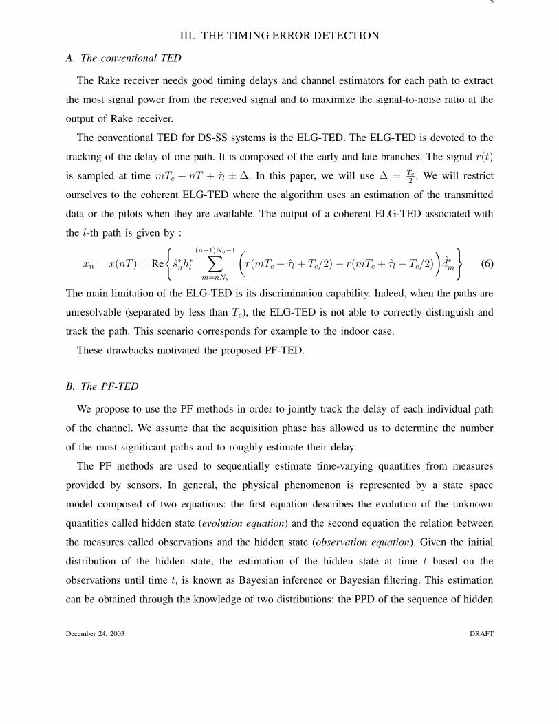
III. THE TIMING ERROR DETECTION
A. The conventional TED
The Rake receiver needs good timing delays and channel estimators for each path to extract
the most signal power from the received signal and to maximize the signal-to-noise ratio at the
output of Rake receiver.
The conventional TED for DS-SS systems is the ELG-TED. The ELG-TED is devoted to the
tracking of the delay of one path. It is composed of the early and late branches. The signal r(t)
is sampled at time mTc + nT + τl ± ∆. In this paper, we will use ∆ = Tc
2. We will restrict
ourselves to the coherent ELG-TED where the algorithm uses an estimation of the transmitted
data or the pilots when they are available. The output of a coherent ELG-TED associated with
the l-th path is given by :
xn = x(nT ) = Re
{
s∗nh∗l
(n+1)Ns−1∑
m=nNs
(
r(mTc + τl + Tc/2) − r(mTc + τl − Tc/2)
)
d∗m
}
(6)
The main limitation of the ELG-TED is its discrimination capability. Indeed, when the paths are
unresolvable (separated by less than Tc), the ELG-TED is not able to correctly distinguish and
track the path. This scenario corresponds for example to the indoor case.
These drawbacks motivated the proposed PF-TED.
B. The PF-TED
We propose to use the PF methods in order to jointly track the delay of each individual path
of the channel. We assume that the acquisition phase has allowed us to determine the number
of the most significant paths and to roughly estimate their delay.
The PF methods are used to sequentially estimate time-varying quantities from measures
provided by sensors. In general, the physical phenomenon is represented by a state space
model composed of two equations: the first equation describes the evolution of the unknown
quantities called hidden state (evolution equation) and the second equation the relation between
the measures called observations and the hidden state (observation equation). Given the initial
distribution of the hidden state, the estimation of the hidden state at time t based on the
observations until time t, is known as Bayesian inference or Bayesian filtering. This estimation
can be obtained through the knowledge of two distributions: the PPD of the sequence of hidden
December 24, 2003 DRAFT

6
states from time 1 to time t given the corresponding sequence of observations and the marginal
distribution of the hidden state at time t given the sequence of the observations until time t. Except
in a few special cases including linear Gaussian state space models, it is impossible to analytically
calculate these distributions. The PF methods provide a discrete and sequential approximation
of the distributions. It can be updated when a new observation is available, without reprocessing
of the previous observations. The support of the distributions is discretized by particles, which
are weighted samples evolving in time.
Tracking the delay of the individual channel paths can be interpreted as a Bayesian inference.
The delays are the hidden state of the system and the model (3) of the received samples relating
the observations to the delays represents the observation equation. We notice that this equation
is nonlinear with respect to the delays and as a consequence, we cannot analytically estimate
the delays. To overcome this nonlinearity, we propose to apply the PF methods.
The PF methods have been previously applied for the delay estimation in DS-CDMA systems
[12], [13]. In [12], the PF methods are used to jointly estimate the data, the channel coefficients
and the propagation delay. In [13], the PF methods are combined with a Kalman Filter (KF) to
respectively estimate the delay propagation and the channel coefficients; the information symbols
are assumed known, provided by a Rake receiver. In both papers, the delays of each channel path
are considered known and multiple of the sampling time; therefore, only the propagation delay is
estimated. In this paper, the approach is different. We suppose that each channel path has a slow
time-varying delay, unknown at the receiver. This environment can represent an indoor wireless
communication. We assume that the information symbols are known or have been estimated
essentially for three reasons:
• To reduce the computational complexity of the receiver;
• The channel estimation is typically performed transmitting known pilot symbols, for example
using a specific channel as the Common Pilot Channel (CPICH) of the UMTS;
• The PF methods applied to the estimation of the information symbols perform slightly worse
than simple deterministic algorithms [12], [14].
Firstly, we will apply the PF methods only to the estimation of the delays of each channel path,
considering that the channel coefficients are known. In the next paragraph, we will introduce the
estimation of the channel coefficients.
The structure of the proposed PF-TED is shown in Fig. 3. This estimator operates on samples
December 24, 2003 DRAFT
7
from the matched filter output taken at an arbitrary sampling rate 1/Ts (at least Nyquist sampling).
Then, the samples are processed by means of interpolation and decimation in order to obtain
intermediate samples at the chip rate 1/Tc. These samples are the input of the particle filter. In
order to reduce the computational complexity of the PF-TED and since the time variation of the
delays are slow with respect to the symbol duration, we choose that the particle filter works at
the symbol rate 1/T . Moreover, in order to exploit all the information contained in the chips of
a symbol period, the equations of the PF algorithm are modified. The PF algorithm proposed in
this paper is thus the adaptation of the PF methods to a DS-SS system.
Following [15], the evolution of the delays of the channel paths can be described as a first
order AutoRegressive (AR) process:
τ1,n = α1τ1,n−1 + v1,n
...
τL,n = αLτL,n−1 + vL,n
, (7)
where τl,n for l = 1, · · · , L denotes the delay of the l-th channel path at time n, α1, · · · , αL
express the possible time variation of the delays from a time to the next one, and v1, · · · , vL
are AWGN with zero mean and variance σ2v . Note that the time index n is an integer multiple
of the symbol duration.
The estimation of the delays can be achieved using the Minimum Mean Square Error (MMSE)
method or the Maximum A Posteriori (MAP) method. The MMSE solution is given by the
following expectation:
τn = E[τn|r1:n], (8)
where τn = {τ1,n, · · · , τL,n} and r1:n is the sequence of received samples from time 1 to n.
The calculation of (8) involves the knowledge of the marginal distribution p(τn|r1:n). Unlike the
MMSE solution that yields an estimate of the delays at each time, the MAP method provides
the estimate of the hidden state sequence τ1:n = {τ1, · · · , τn}:
τ1:n = arg maxτ1:n
p(τ1:n|r1:n). (9)
The calculation of (9) requires the knowledge of the PPD p(τ1:n|r1:n).
The simulations give similar results for the MMSE method and the MAP method. Hence, we
choose to adopt the MMSE solution as in [9]. In order to obtain samples from the marginal
December 24, 2003 DRAFT

8
distribution, we use the Sequential Importance Sampling (SIS) approach [16]. Applying the
definition of the expectation, (8) can be expressed as follows:
τn =
∫
τnp(τn|r1:n)dτn. (10)
The aim of the SIS technique is to approximate the marginal distribution p(τn|r1:n) by means
of weighted particles:
p(τn|r1:n) ≈
Np∑
i=1
w(i)n δ(τn − τ (i)
n ), (11)
where Np is the number of particles, w(i)n is the normalized importance weight at time n associated
with the particle i and δ(τn − τ(i)n ) denotes the Dirac delta centered in τn = τ
(i)n .
The phases of the PF-TED based on the SIS approach are summarized below.
1. Initialization: In this paper, we apply the PF methods for the tracking phase, assuming
that the number of the channel paths and the initial value of the delay for each path have been
estimated during the acquisition phase [17]. We assume that the error on the delay estimated
by the acquisition phase belongs to the interval (−Tc/2, Tc/2). Hence, the a priori probability
density p(τ0) can be considered uniformly distributed in (τ0 − Tc/2, τ0 + Tc/2), where τ0 is the
delay provided by the acquisition phase. Note that the PF methods can be used also for the
acquisition phase. However, the number of particles has to be increased, because we have no a
priori information on the initial value of the delays.
2. Importance sampling: The time evolution of the particles is achieved with an importance
sampling distribution. When rn is observed, the particles are drawn according to the importance
function. In general, the importance function is chosen to minimize the variance of the importance
weights associated with each particle. In fact, it can be shown that the variance of the importance
weights can only increase stochastically over time [16]. This means that, after a few iterations
of the SIS algorithm, only one particle has a normalized weight almost equal to 1 and the other
weights are very close to zero. Therefore, a large computational effort is devoted to updating
paths without almost no contribution to the final estimate. In order to avoid this behavior, a
resampling phase of the particles is inserted among the recursions of the SIS algorithm. To limit
December 24, 2003 DRAFT
9
this degeneracy phenomenon, we need to use the optimal importance function [16], given by:
π(τ (i)n |τ
(i)1:n−1, r1:n) = p(τ (i)
n |τ(i)n−1, rn). (12)
Unfortunately, the optimal importance function can be analytically calculated only in a few
cases, including the class of models represented by a Gaussian state space model with linear
observation equation. In this case, the observation equation (3) is nonlinear and thus, the optimal
importance function cannot be analytically determined. We can consider two solutions to this
problem [16]:
1) the a priori importance function p(τ(i)n |τ
(i)n−1);
2) an approximated expression of the optimal importance function by linearization of the
observation equation about τ(i)l,n = αlτ
(i)l,n−1 for l = 1, · · · , L.
Since the second solution involves the derivative calculation of the nonlinear observation equation
and hence very complex operations, we choose the a priori importance function as in [9].
Considering that the noises vl,n for l = 1, · · · , L in (7) are Gaussian, the importance function
for each delay l is a Gaussian distribution with mean αlτ(i)l,n−1 and variance σ2
v .
3. Weight update: The evaluation of the importance function for each particle at time n enables
the calculation of the importance weights [16]:
w(i)n = w
(i)n−1
p(rn|τ(i)n )p(τ
(i)n |τ
(i)n−1)
π(τ(i)n |τ
(i)1:n−1, r1:n)
. (13)
This expression represents the calculation of the importance weights if we only consider the
samples of the received signal at the symbol rate. However, in a DS-SS system we have additional
information provided by Ns samples for each symbol period due to the spreading sequence.
Consequently, we modify (13) taking into account the presence of a spreading sequence. Indeed,
observing that the received samples are independent, the probability density p(rn|τ(i)n ) at the
symbol rate can be written as:
p(rn|τ(i)n ) =
(n+1)Ns−1∏
m=nNs
p(rm|τ(i)n ). (14)
Considering (3) at the chip rate and recalling the assumptions of known symbols, the probability
density p(rm|τ(i)n ) is Gaussian. Typically, the received sample rm is complex. For the calculation
December 24, 2003 DRAFT
10
of the Gaussian distribution, we can write rm as a bi-dimensional vector with components being
the real part and the imaginary part of rm. The probability density p(rm|τ(i)n ) is thus given by:
p(rm|τ(i)n ) =
1
πσ2n
exp
{
−1
σ2n
∣
∣rm − µ(i)m
∣
∣
2}
, (15)
where σ2n is the variance of the AWGN n(t) in (3) and the mean µ
(i)m is obtained by:
µ(i)m =
L∑
l=1
hl,nsn
m+3∑
k=m−3
dkRg(mTc − kTc − nT − τ(i)l,n). (16)
In order to reduce the computational complexity of the PF-TED, in (16) we have assumed that
the contribution of the raised cosine filter Rg to the sum on the spreading sequence is limited
to the previous 3 and next 3 samples. By substitution of (15) in (14), (14) becomes:
p(rn|τ(i)n ) =
(
1
πσ2n
)Ns
exp
{
−1
σ2n
(n+1)Ns−1∑
m=nNs
∣
∣rm − µ(i)m
∣
∣
2}
. (17)
Assuming the a priori importance function, (13) yields:
w(i)n = w
(i)n−1p(rn|τ
(i)n ) = w
(i)n−1
(
1
πσ2n
)Ns
exp
{
−1
σ2n
(n+1)Ns−1∑
m=nNs
∣
∣rm − µ(i)m
∣
∣
2}
. (18)
Finally, the importance weights in (18) are normalized using the following expression:
w(i)n =
w(i)n
∑Np
j=1 w(j)n
. (19)
4. Estimation: By substitution of (11) into (10), we obtain at each time the MMSE estimate:
τn =
Np∑
i=1
w(i)n τ (i)
n . (20)
5. Resampling: This algorithm presents a degeneracy phenomenon. After a few iterations of the
algorithm, only one particle has a normalized weight almost equal to 1 and the other weights
are very close to zero. This problem of the SIS method can be eliminated with a resampling of
the particles. A measure of the degeneracy is the effective sample size Neff , estimated by:
Neff =1
∑Np
i=1(w(i)n )2
. (21)
When Neff is below a fixed threshold Nthres, the particles are resampled according to the weight
distribution [16]. After each resampling task, the normalized weights are initialized to 1/Np.
December 24, 2003 DRAFT
11
IV. THE ESTIMATION OF THE CHANNEL COEFFICIENTS
A. The conventional estimators
Channel estimation is performed using the known pilot symbols. If we suppose that the channel
remains almost unchanged during the slot, the conventional estimator of the channel coefficients
of the lth path is obtained by correlation using the known symbols [18]:
hl =1
NpilotNs
Npilot−1∑
n=0
Ns−1∑
m=0
s∗nd∗mr(mTc + nT + τl,n), (22)
where Npilot is the number of pilots in a slot. For each path, the received signal is sampled at
time mTc + nT + τl,n in order to compensate its delay. Then the samples are multiplied by the
despread sequence and summed on the whole sequence of pilot symbols. The problem of this
estimator is that when the delays are unresolvable, the estimation becomes biased. To eliminate
this bias, we can use an estimator based on the Maximum Likelihood (ML) criterion. In [19] [1],
a simplified version of the ML estimation is proposed. The channel coefficients which maximize
the ML criterion are given by :
h = P−1
a (23)
where h = (h1, . . . , hL), P is a L × L matrix with elements Pij = Rg(τi,n − τj,n) and a is the
vector of the channel coefficients calculated using (22).
B. The PF-based joint estimation of the delays and the channel coefficients
We can apply the PF methods to jointly estimate the delays of each path and the channel
coefficients with a very low additional cost in terms of computational complexity. This is a
suboptimal solution, since the observation equation (3) is linear and Gaussian with respect to
the channel coefficients. The optimal solution is represented by a Kalman Filter (KF). However,
combining the PF methods and the KF to jointly estimate the delays and the channel coefficients
involves the implementation of a KF. It is better to use the particles employed for the delay
estimation and to associate to each particle the estimation of the channel coefficients.
In this case, the hidden state is composed of the L delays and the L channel coefficients of
each individual path. When a particle evolves in time, its new position is thus determined by
the evolution of the delays and the evolution of the channel coefficients. The delays evolve as
described for the PF-TED. For the channel coefficients, we assume that the time variations are
December 24, 2003 DRAFT

12
slow as for example in indoor environments. Hence, the evolution of the channel coefficients
can be expressed by the following first order AR model:
h1,n = β1h1,n−1 + z1,n
...
hL,n = βLhL,n−1 + zL,n
, (24)
where β1, · · · , βL describe the possible time variation of the channel coefficients from a time to
the next one and z1, · · · , zL are AWGN with zero mean and variance σ2z . Notice that this joint
estimator operates at the symbol rate as the PF-TED.
As for the delays, we only consider the MMSE method for the estimation of the channel
coefficients and we use a prior importance function:
π(h(i)n |h
(i)1:n−1, r1:n) = p(h(i)
n |h(i)n−1), (25)
where hn = {h1,n, · · · , hL,n}. Considering that the noises zl,n for l = 1, · · · , L in (24) are
Gaussian, the importance function for the channel coefficients is a Gaussian distribution with
mean βlh(i)l,n−1 and variance σ2
z . To determine the positions of the particles at time n from the
positions at time n − 1, each particle is drawn according to p(τ(i)n |τ
(i)n−1) and (25).
The calculation of the importance weights is very similar to the case of the PF-TED. The
only difference is that the channel coefficients hl,n are replaced by the support of the particles
h(i)l,n.
V. SIMULATION RESULTS
In this section, we will compare the performance of the conventional ELG-TED and the
PF-TED. In order to demonstrate the gain achieved using the latter, we will consider different
indoor scenarios with a two Rayleigh path channel with the same average power on each path
and a maximum Doppler frequency of 19 Hz corresponding to a mobile speed of 10 Km/h for
a carrier frequency of 2GHz. The simulation setup is compatible with the UMTS standard. In
these conditions, the time variations of the channel delays can be expressed by the model (7),
with α1 = · · · = αL = 0.99999 and σ2v = 10−5 [15]. Moreover, the time variations of the channel
coefficients can be represented by the model (24), β1 = · · · = βL = 0.999 and σ2z = 10−3.
December 24, 2003 DRAFT
13
In these simulations, a CPICH is used. In each slot of CPICH, 40 pilot symbols equal to 1
are expanded into a chip level by a spreading factor of 64. The spreading sequence is a PN
sequence changing at each symbol.
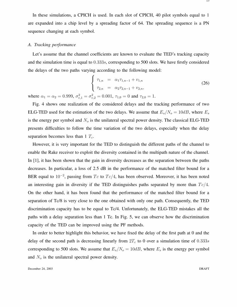
A. Tracking performance
Let’s assume that the channel coefficients are known to evaluate the TED’s tracking capacity
and the simulation time is equal to 0.333s, corresponding to 500 slots. We have firstly considered
the delays of the two paths varying according to the following model:
τ1,n = α1τ1,n−1 + v1,n
τ2,n = α2τ2,n−1 + v2,n,(26)
where α1 = α2 = 0.999, σ2v,1 = σ2
v,2 = 0.001, τ1,0 = 0 and τ2,0 = 1.
Fig. 4 shows one realization of the considered delays and the tracking performance of two
ELG-TED used for the estimation of the two delays. We assume that Es/No = 10dB, where Es
is the energy per symbol and No is the unilateral spectral power density. The classical ELG-TED
presents difficulties to follow the time variation of the two delays, especially when the delay
separation becomes less than 1 Tc.
However, it is very important for the TED to distinguish the different paths of the channel to
enable the Rake receiver to exploit the diversity contained in the multipath nature of the channel.
In [1], it has been shown that the gain in diversity decreases as the separation between the paths
decreases. In particular, a loss of 2.5 dB in the performance of the matched filter bound for a
BER equal to 10−2, passing from Tc to Tc/4, has been observed. Moreover, it has been noted
an interesting gain in diversity if the TED distinguishes paths separated by more than Tc/4.
On the other hand, it has been found that the performance of the matched filter bound for a
separation of Tc/8 is very close to the one obtained with only one path. Consequently, the TED
discrimination capacity has to be equal to Tc/4. Unfortunately, the ELG-TED mistakes all the
paths with a delay separation less than 1 Tc. In Fig. 5, we can observe how the discrimination
capacity of the TED can be improved using the PF methods.
In order to better highlight this behavior, we have fixed the delay of the first path at 0 and the
delay of the second path is decreasing linearly from 2Tc to 0 over a simulation time of 0.333s
corresponding to 500 slots. We assume that Es/No = 10dB, where Es is the energy per symbol
and No is the unilateral spectral power density.
December 24, 2003 DRAFT
14
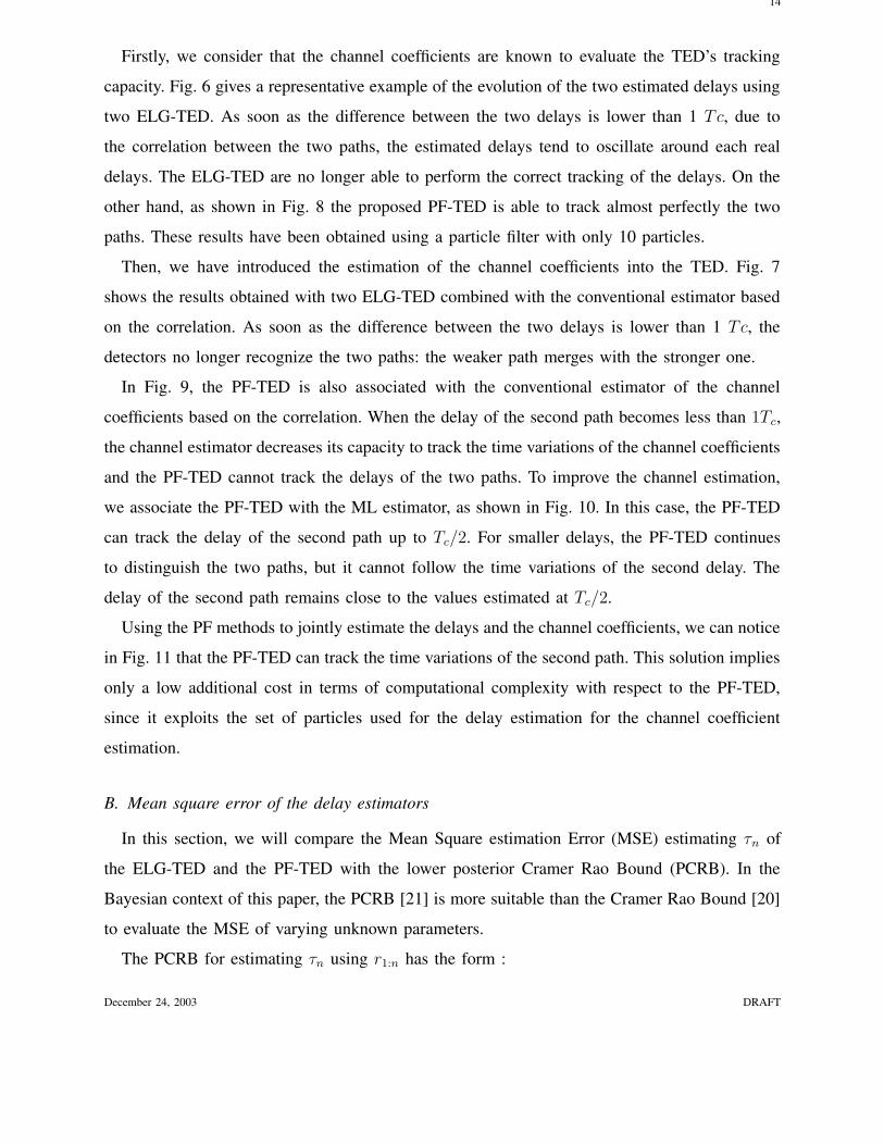
Firstly, we consider that the channel coefficients are known to evaluate the TED’s tracking
capacity. Fig. 6 gives a representative example of the evolution of the two estimated delays using
two ELG-TED. As soon as the difference between the two delays is lower than 1 Tc, due to
the correlation between the two paths, the estimated delays tend to oscillate around each real
delays. The ELG-TED are no longer able to perform the correct tracking of the delays. On the
other hand, as shown in Fig. 8 the proposed PF-TED is able to track almost perfectly the two
paths. These results have been obtained using a particle filter with only 10 particles.
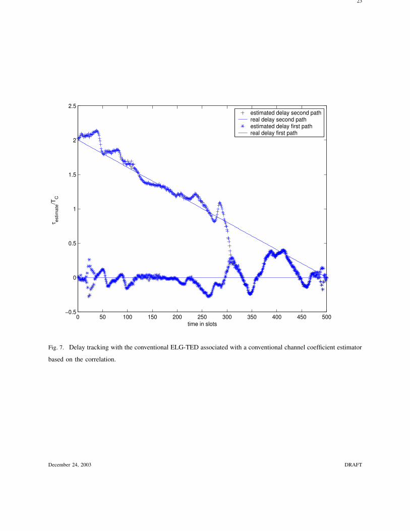
Then, we have introduced the estimation of the channel coefficients into the TED. Fig. 7
shows the results obtained with two ELG-TED combined with the conventional estimator based
on the correlation. As soon as the difference between the two delays is lower than 1 Tc, the
detectors no longer recognize the two paths: the weaker path merges with the stronger one.
In Fig. 9, the PF-TED is also associated with the conventional estimator of the channel
coefficients based on the correlation. When the delay of the second path becomes less than 1Tc,
the channel estimator decreases its capacity to track the time variations of the channel coefficients
and the PF-TED cannot track the delays of the two paths. To improve the channel estimation,
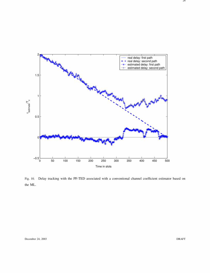
we associate the PF-TED with the ML estimator, as shown in Fig. 10. In this case, the PF-TED
can track the delay of the second path up to Tc/2. For smaller delays, the PF-TED continues
to distinguish the two paths, but it cannot follow the time variations of the second delay. The
delay of the second path remains close to the values estimated at Tc/2.
Using the PF methods to jointly estimate the delays and the channel coefficients, we can notice
in Fig. 11 that the PF-TED can track the time variations of the second path. This solution implies
only a low additional cost in terms of computational complexity with respect to the PF-TED,
since it exploits the set of particles used for the delay estimation for the channel coefficient
estimation.
B. Mean square error of the delay estimators
In this section, we will compare the Mean Square estimation Error (MSE) estimating τn of
the ELG-TED and the PF-TED with the lower posterior Cramer Rao Bound (PCRB). In the
Bayesian context of this paper, the PCRB [21] is more suitable than the Cramer Rao Bound [20]
to evaluate the MSE of varying unknown parameters.
The PCRB for estimating τn using r1:n has the form :
December 24, 2003 DRAFT
15
E(τn − τn)2 ≥ J−1n,n (27)
where Jn,n is the right lower element of the n × n Fisher information matrix.
In [21], the authors have shown how to evaluate recursively Jn,n. For our application, the
nonlinear filtering system is
τn+1 = ατn + vn
rn = zn(τn) + nn,(28)
where the second relation represents the nonlinear observation equation (3) at chip rate.
Since the spreading sequence is different at each chip time, we have to evaluate zn(τn) at this
rate.
From the general recursive equation given in [21] the sequence {Jn,n} can be obtained as
follows :
Jn+1,n+1 = σ−1v + E[Oτn+1
zn+1(τn+1)]2σ−1
n − (ασ−1v )2(Jn,n + α2σ−1
v )−1 (29)
In order to calculate E[Oτn+1zn+1(τn+1)], we have applied a Monte Carlo evaluation. We
generate M i.i.d. state trajectories of a given length Nt {τ i0, τ
i1, . . . τ
iNt} with 1 ≤ i ≤ M by
simulating the system model defined in (28) starting from an initial state τ0 drawn from the a
priori probability density p(τ0). For the calculation, we fixed M = 100.
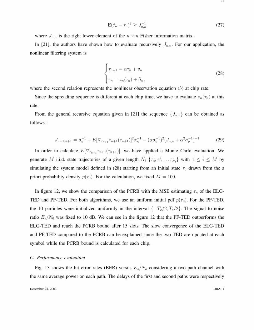
In figure 12, we show the comparison of the PCRB with the MSE estimating τn of the ELG-
TED and PF-TED. For both algorithms, we use an uniform initial pdf p(τ0). For the PF-TED,
the 10 particles were initialized uniformly in the interval {−Tc/2, Tc/2}. The signal to noise
ratio Es/N0 was fixed to 10 dB. We can see in the figure 12 that the PF-TED outperforms the
ELG-TED and reach the PCRB bound after 15 slots. The slow convergence of the ELG-TED
and PF-TED compared to the PCRB can be explained since the two TED are updated at each
symbol while the PCRB bound is calculated for each chip.
C. Performance evaluation
Fig. 13 shows the bit error rates (BER) versus Es/No considering a two path channel with
the same average power on each path. The delays of the first and second paths were respectively
December 24, 2003 DRAFT
16
fixed at 0 and 1 Tc. The same maximum Doppler frequency as above was used. The BER values
have been averaged over 50000 bits.
When using two ELG-TED, except when the channel is known the performance are very poor
compare to the maximum achievable performance (known delays and channel coefficients). On
the other hand, the PF-TED with channel coefficients known or estimated reaches the optimal
performance. We can conclude that the considered TED must be able to separate the different
paths of the channel, otherwise the performance of the Rake receiver breaks down.
VI. CONCLUSIONS
In this paper we have proposed to use the PF methods in order to track the delay of the
different channel paths. We have assumed that an acquisition phase has already provided an
initial estimation of these delays.
We have firstly considered that the channel coefficients are known. We have compared the
tracking capacity of the conventional ELG-TED and the proposed PF-TED. We have shown that
when the delays of the channel paths become very close (less than 1Tc), the ELG-TED is unable
to track the time variations of the delays. However, the PF-TED continues to track the delays.
We have introduced the channel coefficient estimation to the TED. We have considered two
classical methods: the estimation based on the correlation using pilot symbols and the estimation
based on the ML criterion. We have shown that the ELG-TED with estimation of the channel
coefficients loses the capacity to distinguish the paths when the delays are very closed. On the
other hand, the PF-TED associated with the two classical channel estimator is able to separate
the different paths. However, for very close delays the channel estimators prevent to the PF-TED
to track the time variations of the delays. We have proposed to estimate jointly the delays and
the channel coefficients using the PF methods to avoid this loss of tracking. We have found that
the joint estimation enables a better tracking of the delays.
Finally, we have seen that it is very important for the Rake receiver that the TED can
distinguish the different paths of the channel. We have observed that in the case of unresolvable
paths, the ELG-TED confuses the paths and the performance of the Rake receiver are very poor.
As conclusion, we can say that the PF-TED based on the joint estimation of the delays
and the channel coefficients can be a good substitute of the classical ELG-TED, specially for
December 24, 2003 DRAFT
17
indoor wireless communications. Moreover, the computational complexity of the PF-TED is very
limited, seen that we have used only 10 particles.
REFERENCES
[1] H. Boujemaa, M. Siala, “Rake receivers for direct sequence spread spectrum systems,” Ann. Telecommun., Vol. 56, No. 5-6,
pp. 291–305, 2001.
[2] V. Aue, G. P. Fettweis, “A non-coherent tracking scheme for the Rake receiver that can cope with unresolvable multipath,”
ICC 1999, June 1999.
[3] R. De Gaudenzi, “Direct-sequence spread spectrum chip tracking in the presence of unresolvable multipath components,”
IEEE Transactions on Vehicular Technology, Vol. 48, pp. 1573–1583, September 1999.
[4] G. Fock, J. Baltersee, P. Schulz-Rittich, and H. Meyr, “ Channel tracking for Rake receivers in closely spaced multipath
environments,” IEEE Journal on Selected Areas in Communications, Vol. 19, pp. 2420-2431, December 2001.
[5] A. Doucet, J. F. G. de Freitas, and N. J. Gordon, Sequential Monte Carlo methods in practice. New York: Springer-Verlag,
2001.
[6] J. S. Liu and R. Chen, “Blind deconvolution via sequential imputations,” Journal of the American Statistical Association,
Vol. 90, Issue 430, pp. 567–576, June 1995.
[7] R. Chen, X. Wang, and J. S. Liu, “Adaptive joint detection and decoding in flat-fading channels via mixture Kalman
filtering,” IEEE Transactions on Information Theory, Vol. 46, No.6, pp. 2079–2094, September 2000.
[8] E. Punskaya, C. Andrieu, A. Doucet, and W. J. Fitzgerald, “Particle filtering for demodulation in fading channels with
non-Gaussian additive noise,” IEEE Transactions on Communications, Vol. 49, No.4, pp. 579–582, April 2001.
[9] T. Ghirmai, M. F.Bugallo, J. Mıguez, and P. M. Djuric, “Joint symbol detection and timing estimation using particle
filtering,” Proceedings of ICASSP, Vol. 4, pp. 596–599 6–10 April 2003.
[10] P. M. Djuric, J. H. Kotecha, J. Zhang, Y. Huang, T. Ghirmai, M. F.Bugallo, and J. Mıguez, “Applications of particle .ltering
to selected problems in communications,” IEEE Signal Processing Magazine, September 2003.
[11] 3GPP Technical Specification Group Radio Access Network, Spreading and Modulation (FDD), 3G TS 25.213 version
3.3.0, December 2000.
[12] E. Punskaya, A. Doucet, and W. J. Fitzgerald, “On the use and misuse of particle filtering in digital communications,”
EUSIPCO 2002, Toulouse, September 2002.
[13] R. A. Iltis, “A sequential Monte Carlo filter for joint linear/nonlinear state estimation with application to DS-CDMA,”
IEEE Transactions on Signal Processing, Vol. 51, pp. 417–426, February 2003.
[14] T. Bertozzi, D. Le Ruyet, G. Rigal, and H. Vu-Thien, “On particle filtering in digital communications,” SPAWC 2003,
Rome, June 2003.
[15] R. A. Iltis, “Joint estimation of PN code delay and multipath using the extended Kalman filter,” IEEE Transactions on
Communications, Vol. 38, pp. 1677–1685, October 1990.
[16] A. Doucet, S. Godsill, and C. Andrieu, “On sequential Monte Carlo sampling methods for Bayesian filtering,” Statistics
and Computing, Vol. 10, No. 3, pp. 197–208, 2000.
[17] A. J. Viterbi, CDMA : principles of spread spectrum communication. Ed. Addison-Wesley, June 1995.
[18] H. Meyr, M. Moeneclaey, and S. Fechtel, Digital Communication receivers. Ed. Wiley Series in Telecom and Signal
Processing, 2nd Edition, New York, 1998.
December 24, 2003 DRAFT
18
[19] E. Sourour, G. Bottomley, and R. Ramesh, “Delay tracking for direct sequence spread spectrum systems in multipath
fading channels”Vehicular Technology Conference Spring VTC’99, Amsterdam, Vol. 1, pp. 422–426, 1999.
[20] U. Mengali and A. N. D’Andrea, Synchronization Techniques for Digital Receivers . Plenun Press, New York, 1997.
[21] P. Tichavsky, C. H. Muravchik, and A. Nehorai. “Posterior Cramer-Rao Bounds for Discrete-Time Nonlinear Filtering”.
IEEE Transactions on Signal Processing, Vol. 46-5, pp. 1386–1396, May 1998.
[22] N. Bergman, L. Ljung, and F. Gustafsson, “Terrain navigation using Bayesian statistics” IEEE Control Systems Magazine,
Amsterdam, Vol. 19, No. 3, pp. 33–40, 1999.
December 24, 2003 DRAFT

19
n s
m d
) ( t g
) ( t n
) ( t r
CHANNEL
) , ( t h ) ( * t g
Fig. 1. Equivalent lowpass transmission system model.
r(t)
) ( ˆ 1 t mT nT
1
0
S N
m
* ˆ m d *
1 ˆ h
* ˆ m d * ˆ
L h
1/T S
Interpolator/ Decimator
Interpolator/ Decimator
) ( ˆ t mT nT
N S
1
1
0
S N
m N S
1
L
C
C
n s ˆ
Fig. 2. Rake receiver model.
) ( t r s T / 1
Interpolator/ Decimator
) ( c mT r Particle Filter 1
) ( nT ) ( nT L , ,
Fig. 3. Structure of the proposed PF-TED.
December 24, 2003 DRAFT

20
0 50 100 150 200 250 300 350 400 450 500−0.4
−0.2
0
0.2
0.4
0.6
0.8
1
1.2
1.4
1.6
Time in slots
τ estim
ate/T
c
true delay
estimated delay
Fig. 4. Delay tracking with the conventional ELG-TED.
December 24, 2003 DRAFT

21
0 50 100 150 200 250 300 350 400 450 500−0.2
0
0.2
0.4
0.6
0.8
1
1.2
1.4
Time in slots
τ estim
ate/T
c
true delay
estimated delay
Fig. 5. Delay tracking with the PF-TED.
December 24, 2003 DRAFT

22
0 50 100 150 200 250 300 350 400 450 500−0.5
0
0.5
1
1.5
2
2.5
time in slots
τ estim
ate/T
C
estimated delay second pathreal delay second pathestimated delay first pathreal delay first path
Fig. 6. Delay tracking with the conventional ELG-TED.
December 24, 2003 DRAFT
23
0 50 100 150 200 250 300 350 400 450 500−0.5
0
0.5
1
1.5
2
2.5
time in slots
τ estim
ate/T
C
estimated delay second pathreal delay second pathestimated delay first pathreal delay first path
Fig. 7. Delay tracking with the conventional ELG-TED associated with a conventional channel coefficient estimator
based on the correlation.
December 24, 2003 DRAFT

24
0 50 100 150 200 250 300 350 400 450 500−0.5
0
0.5
1
1.5
2
2.5
Time in slot
τ estim
ate/T
c
real delay: first pathreal delay: second pathestimated delay: first pathestimated delay: second path
Fig. 8. Delay tracking with the PF-TED.
December 24, 2003 DRAFT

25
0 50 100 150 200 250 300 350 400 450 500−0.5
0
0.5
1
1.5
2
2.5
Time in slots
τ estim
ate/T
c
real delay:first pathreal delay: second pathestimated delay: first pathestimated delay: second path
Fig. 9. Delay tracking with the PF-TED associated with a conventional channel coefficient estimator based on the
correlation.
December 24, 2003 DRAFT
26
0 50 100 150 200 250 300 350 400 450 500−0.5
0
0.5
1
1.5
2
Time in slots
τ estim
ate/T
c
real delay: first pathreal delay: second pathestimated delay: first pathestimated delay: second path
Fig. 10. Delay tracking with the PF-TED associated with a conventional channel coefficient estimator based on
the ML.
December 24, 2003 DRAFT

27
0 50 100 150 200 250 300 350 400 450 500−0.5
0
0.5
1
1.5
2
2.5
Time in slots
τ estim
ate/T
c
real delay: first pathreal delay: second pathsestimated delay: first pathestimated delay: second path
Fig. 11. Delay tracking with a joint delay and channel coefficient estimator based on the PF methods.
December 24, 2003 DRAFT

28
0 2 4 6 8 10 12 14 16 18 200
0.02
0.04
0.06
0.08
0.1
0.12
0.14
0.16
0.18
0.2
Mea
n S
quar
e E
rror
PF−TEDPCRBELG−TED
time in slots
Fig. 12. Comparison of the PCRB with the MSE estimating τn of ELG-TED and PF-TED
December 24, 2003 DRAFT

29
0 2 4 6 8 10 1210−3
10−2
10−1
100
Es/N
0 (dB)
BE
R
Rake known del. known chan.ELG−TED known chan.PF−TED known chan.ELG−TED estim. chan. corr.PF−TED estim.chan. corr.PF−TED estim. chan. PF
Fig. 13. Performance comparison of the ELG-TED and the PF-TED.
December 24, 2003 DRAFT


