
Chaos, Solitons and Fractals 102 (2017) 245–253
Contents lists available at ScienceDirect
Chaos, Solitons and Fractals
Nonlinear Science, and Nonequilibrium and Complex Phenomena
journal homepage: www.elsevier.com/locate/chaos
Pricing of basket options in subdiffusive fractional Black–Scholes
model
Gulnur Karipova, Marcin Magdziarz
∗
Faculty of Pure and Applied Mathematics, Hugo Steinhaus Center, Wroclaw University of Science and Technology, Wyspianskiego 27, 50-370 Wroclaw,
Poland
a r t i c l e i n f o
Article history:
Received 26 January 2017
Revised 4 May 2017
Accepted 5 May 2017
Available online 10 May 2017
Keywords:
Black–Scholes model
Subdiffusion
Basket options
Stable process
a b s t r a c t
In this paper we generalize the classical multidimensional Black-Scholes model to the subdiffusive case.
In the studied model the prices of the underlying assets follow subdiffusive multidimensional geometric
Brownian motion. We derive the corresponding fractional Fokker–Plank equation, which describes the
probability density function of the asset price. We show that the considered market is arbitrage-free and
incomplete. Using the criterion of minimal relative entropy we choose the optimal martingale measure
which extends the martingale measure from used in the standard Black–Scholes model. Finally, we derive
the subdiffusive Black–Scholes formula for the fair price of basket options and use the approximation
methods to compare the classical and subdiffusive prices.
© 2017 Elsevier Ltd. All rights reserved.
1
t
t
h
M
t
t
m
t
o
s
t
p
T
a
S
u
p
a
w
e
m
d
[
t
F
t
B
t
i
m
p
o
m
W
t
b
o
s
p
fi
u
t
h
0
. Introduction
During the last few decades the scientists have had a keen in-
erest to the problem of financial markets’ modelling and deriva-
ion of prices of different financial derivatives. The breakthrough
appened when in 1973 the papers of Black and Scholes [1] and
erton [14] were published. These papers had a great impact to
he financial market and arouse huge academic interest, setting up
he key principles of arbitrage option pricing. However, the original
odel has its disadvantages as it sets a number of restrictions on
he real state of life [19] . Many of assumptions were relaxed in the
ngoing researches. In this work the subdiffusive phenomena is of
pecific interest.
The fact is that in some financial markets the number of par-
icipants and, therefore, performed transactions, is so low that the
rice of the asset may remain constant during the period of time.
his phenomenon is the most inherent for the emerging markets
nd it breaks the assumption on liquidity set in the original Black–
choles (B-S) model. The idea to model the price of such assets
sing subdiffusive Geometric Brownian Motion (GBM) comes from
hysics: the so-called stagnation periods in the market are associ-
ted with the trapping events of the subdiffusive test particle [4] ,
hich is manifested by the fractional derivatives in Fokker–Planck
quations [15,16] .
∗ Corresponding author.
E-mail addresses: [email protected] (G. Karipova),
[email protected] (M. Magdziarz).
a
B
o
B
ttp://dx.doi.org/10.1016/j.chaos.2017.05.013
960-0779/© 2017 Elsevier Ltd. All rights reserved.
The generalized to the subdiffusive regime B-S model for one
imensional case was already introduced in details in the literature
9] . However, such model cannot define the price of such impor-
ant financial derivatives as, for instance, European basket options.
or these reasons the multidimensional B-S model was applied in
he standard approach. Here we generalize the multidimensional
-S model by adding the periods of stagnation, which are charac-
eristic for subdiffusion and can be modelled by equations involv-
ng fractional derivatives. We underline the extension from one- to
ultidimensional setting of the subdiffusive B-S model is at some
oints not straightforward. Property of lack of arbitrage depends
n the parameters of the volatility matrix. Also, the martingale
easure is not unique, its choice has crucial influence on the price.
e use the relative entropy criterion to solve this problem. Addi-
ionally, there is no closed-form formula for the fair price of the
asket option. It has to be approximated using Monte Carlo meth-
ds or applying deterministic approach.
Let us remind that the celebrated B-S formula was derived by
olving certain heat equation, so the motivation came clearly from
hysics. We expect that the similar process will be observed in
nancial engineering. Fractional operators, which are successfully
sed in statistical physics in the description of anomalous frac-
ional dynamics will find important applications also in finance.
The first chapter of this work includes the basic knowledge
bout the options, classical one-dimensional and multidimensional
-S models and such characteristics of the financial market as lack
f arbitrage and market completeness.
The second chapter introduces the concept of multidimensional
-S model, generalized to the subdiffusive case. At the beginning

246 G. Karipova, M. Magdziarz / Chaos, Solitons and Fractals 102 (2017) 245–253
2
p
e
i
t
T
t
a
s
f
d
o
Z
H
i
C
w
d
H
m
d
h
o
P
T
a
d
p
i
s
2
s
Z
d
o
Z
w
w
a
k
f
s
p
C
the inverse stable subordinator is defined and its basic character-
istics are given. The subdiffusive multidimensional GBM is intro-
duced, i.e. the subordinated process used to model the prices of
the underlying assets with specific periods of stagnation. The frac-
tional multidimensional Fokker–Planck equation is derived, which
gives the information about the dynamics of the probability den-
sity function (PDF) of the studied process [13,15,16] . In the follow-
ing it is proved that the considered market is arbitrage-free and
incomplete. It should be added that the lack of arbitrage for sub-
diffusive B-S model was also analyzed in [7] . The B-S formula of
option pricing is derived, the price of basket call option depending
on the stability parameter α, maturity time and the strike price is
approximated by the methods of numerical integration and Monte-
Carlo simulations. The obtained price functions are compared with
the classical case. We end the paper with concluding chapter.
For the sake of clarity we moved the most technical proofs to
the Appendix .
2. B-S: classical approach
2.1. Options
Let us recall the definition of an option. Option is a financial
instrument such that its buyer (owner) has the right to buy (call
option) or to sell (put option) an asset Z ( t ) at some prespecified
maturity time T for a prespecified strike price K . The underlying
asset is usually a stock but some other assets are also possible. A
European option, in contrary to the American option, can be exer-
cised at the maturity time only, whereas it is possible to exercise
American option at any time up to expiration [1,17] .
The payoffs of the European call option and the European put
option are equal to (Z(T ) − K) + and (K − Z(T )) + , respectively.
Here (x ) + = max (x, 0) . There is a relationship between price of the
put option P and the price of a call option C . This relationship is
called put-call parity [17] :
Z(0) − Ke −rT = C − P. (1)
Here r ≥ is the interest rate. Further on, we will assume for sim-
plicity that r = 0 .
Let us now introduce the concept of a basket option, which is
defined as financial instrument, where the underlying asset is a
portfolio of various assets Z ( i ) ( t ), i = 1 , . . . , m, for instance, single
stocks. Basket option among others belongs to the class of exotic
options. The basket option implies higher cost-effectiveness than a
simple collection of single options, as it is a diversification instru-
ment which also takes into account the interdependences between
diverse risk factors. As an example, there might be a negative cor-
relation between stocks in the “basket”, strong enough to signifi-
cantly reduce the total risk or even make it disappear [17] . Basket
option, exercised in European call style, has the following payoff(
m ∑
i =1
ω i Z (i ) (T ) − K
)
+ , (2)
where { ω i } m
i =1 are constant weights, such that
∑ m
i =1 ω i = 1 . Here
the constant K > 0 is the strike price.
Trading of option contracts has had a long historical life. How-
ever, the prevalence of the option market increased rapidly in 1973
when options regulations became standardized and transactions
on the stock options were performed on the Chicago Board Op-
tions Exchange. Simultaneously in 1973 Black and Scholes [1] and
Merton [14] published their celebrated papers. These papers had
a great impact to the financial market and arouse huge academic
interest, setting up the key principles of arbitrage option pricing.
While the fair prices of European options can be found using
the classical B-S formula, to find the price of a basket option one
needs to use the multidimensional models.
.2. Classical B-S model
Over the last forty years the B-S [2,14,17,19] model is being a
owerful tool for pricing derivatives. One may define it as a math-
matical model that allows us to simulate the prices of financial
nstruments, such as stocks, as well as derive the fair prices of cer-
ain financial derivatives such as European call options.
Let us consider such a market, that its development up to time
is defined on the probability space ( �, F, P ), where � is called
he sample space, F is a set of all events and possible statements
bout the prices on the market and P is the usual probability mea-
ure. The price of an asset Z t in classical B-S model is assumed to
ollow GBM given by
Z t =
(μ +
1
2
σ 2 )
Z t dt + Z t σdW t , Z 0 = z 0 (3)
r equivalently
t = Z 0 exp { μt + σW t } . (4)
ere, W t is the standard Brownian motion with respect to P, σ > 0
s the diffusion (volatility) parameter and μ ∈ R is the drift.
The celebrated B-S price of European call option equals [1] :
B −S (Z 0 , K, T , σ ) = Z 0 �(d + ) − K�(d −) , (5)
ith
± =
log Z 0 K
± 1 2 σ 2 T
σ√
T ,
ere � is the distribution function of Gaussian distribution with
ean zero and variance equal to one. This fair price was originally
erived by Black and Scholes by solving the well-known in physics
eat equation.
By the mentioned put-call parity we have for the price of put
ption
B −S (Z 0 , K, T , σ ) = C B −S (Z 0 , K, T , σ ) + K − Z 0 . (6)
he B-S model was certainly a break-through in the option pricing
pparatus. However, it has number of limiting assumptions that
o not reflect the real market conditions and behavior of assets’
rices. This gives a fruitful area for academic purposes: already ex-
sting and ongoing researches are aimed to possibly relax these as-
umptions.
.3. Multidimensional B-S model
The classical B-S model can be generalized to the multidimen-
ional case, i.e. the number of assets m > 1 and the asset prices
(t) = (Z (1) t , . . . , Z (m )
t ) follow multidimensional GBM as
Z (i ) t =
(
μi +
1
2
n ∑
j=1
σ 2 i j
)
Z (i ) t d t + Z (i )
t
n ∑
j=1
σi j d W
( j) t , Z (i )
0 = z 0 i (7)
r equivalently
(i ) t = Z (i )
0 exp
{
μi t +
n ∑
j=1
σi j W
( j) t
}
, i = 1 , . . . m,
here W (t) = (W
(1) t , . . . , W
(n ) t ) is n -dimensional Brownian motion
ith respect to P , { σ ij } m ×n , σ ij ≥ 0, is non-singular volatility matrix
nd (μ1 , . . . , μm
) is a drift vector.
Multidimensional B-S model allows to find the fair price of bas-
et options defined in (2) . Unfortunately, there is no explicit B-S
ormula for such purpose. The price of a basket option in the clas-
ical multidimensional B-S model can be found using Gentle’s ap-
roximation by geometric average [6,17] . It is given by
B −S =
(
m ∑
i =1
ω i Z (i ) 0
)
(c�(l 1 (T )) − ( K + c − 1)�(l 2 (T ))) , (8)

G. Karipova, M. Magdziarz / Chaos, Solitons and Fractals 102 (2017) 245–253 247
w
c
v
ρ
ω
w
l
2
m
p
[
Z
P
Q
a
i
t
r
p
fi
P
t
s
i
g
i
Q
e
l
r
I
Q
s
t
t
3
d
[
t
F
t
s
o
t
i
m
o
P
h
t
t
t
i
b
t
c
3
S
0
L
E
i
h
s
E
w
o
E
w
f
S
o
o
3
d
Z
w
c
d
c
o
r
F
t
here
= exp
{ (
1
2
v 2 − 1
2
m ∑
j=1
ˆ ω j σ2 j
)
T
}
,
2 =
m ∑
i, j=1
ρi, j ω i ω j σi σ j ,
i, j =
∑ n k =1 σik σ jk
σi σ j
, σi =
√
n ∑
k =1
σ 2 ik ,
ˆ i =
ω i Z (i ) 0 ∑ m
j=1 ω j Z ( j) 0
, K =
K ∑ m
j=1 ω j Z ( j) 0
,
here { ρ ij } m ×n are the instantaneous correlation coefficients and
1 , 2 (t) =
ln c − ln ( K + c − 1) ± 1 2 v 2 t
v √
t .
.4. Arbitrage free market and market completeness
The lack of arbitrage for a market model is crucial require-
ent for pricing regulations, i.e. it should not be possible to get a
rofit without any risk. The Fundamental Theorem of Asset Pricing
3] states that the market model is arbitrage-free if the asset price
( t ) is a martingale with respect to some measure Q equivalent to
. In other words, Z ( t ) is a fair-game process w.r.t. Q . The measure
is such a measure under which the expected rate of return on
ll assets existing in arbitrage-free market is equal for all financial
nstruments despite the variability of assets’ price, whereas under
he real-life measure P the higher is the risk, the larger is expected
ate of return [9] .
Another vital characteristic of the market model is market com-
leteness which assures the uniqueness of the fair price for each
nancial instrument. The Second Fundamental Theorem of Asset
ricing [3] states that if there is only one martingale measure Q
hen the market is complete.
One can show that the classical one-dimensional B-S model re-
ponds to both arbitrage-free and completeness criteria, therefore,
ts B-S formula for option pricing defines a unique fair price of sin-
le European option. The martingale measure Q for the B-S model
s given by
(A ) =
∫ A
exp
{
−(μ + σ 2 / 2
σ
)2 T
2
− μ + σ 2 / 2
σW T
}
dP, A ∈ F .
(9)
In the multidimensional B-S model the case looks a bit differ-
nt. Let us introduce constants { γ j } n j=1 as the solution of the fol-
owing system
− μi −1
2
n ∑
j=1
σ 2 i j =
n ∑
j=1
σi j γ j , i = 1 , . . . m, (10)
f the solution of such system exists, then there exists Q defined as
(A ) =
∫ A
exp
{
−n ∑
i =1
γi W
(i ) T
− 1
2
n ∑
i =1
γ 2 i T
}
dP, A ∈ F , (11)
uch that Z ( t ) is a martingale w.r.t. Q . This implies the lack of arbi-
rage. One can show that the considered market model is complete,
herefore, all financial derivatives have unique fair prices.
. Subdiffusive multidimensional B-S model
The generalized to the subdiffusive regime B-S model for one
imensional case was already introduced in details in the literature
9] . However, such model cannot define the price of such impor-
ant financial derivatives as, for instance, European basket options.
or these reasons the multidimensional B-S model was applied in
he classical approach.
The following chapter introduces the concept of multidimen-
ional B-S model, generalized to the subdiffusive case. It consists
f three sections. The first defines the inverse α-stable subordina-
or and gives its basic characteristics. The second introduces subd-
ffusive multidimensional GBM, i.e. subordinated process used to
odel the prices of the underlying assets with specific periods
f stagnation. There is also a fractional multidimensional Fokker–
lank equation derived, which gives the information about the be-
avior of the PDF of the studied process [13,15,16] . The third sec-
ion shows that the introduced subdiffusive market has no arbi-
rage and is not complete. The subdiffusive B-S formula of op-
ion pricing is derived here, the price of basket options depend-
ng on the α, maturity time and the strike price is approximated
y the methods of numerical integration and Monte-Carlo simula-
ions. The obtained price functions are compared with the classical
ase.
.1. Inverse alpha-stable subordinator
The inverse α-stable subordinator is defined as
α(t) = inf { τ > 0 : U α(τ ) > t} , (12)
< α < 1. Here { U α( τ )} τ > 0 is the strictly increasing α-stable
évy process (subordinator). It has the following Laplace transform
(e −uU α (t) ) = e −tu α [8,22,23] . Here E denotes the expectation. Us-
ng the fact that U α( t ) is 1/ α-self-similar process, we get that S α( t )
as the same distribution as [ t / U α(1)] α . The moments of the con-
idered process can be found in [12]
[ S n α(t )] =
t nαn !
(nα + 1) , (13)
here ( ·) is the gamma function. Moreover, the Laplace transform
f S α( t ) equals
(e −uS α (t) ) = E α(−ut α) , (14)
here the function E α(z) =
∑ ∞
n =0 z n
(nα+1) is the Mittag-Leffler
unction [11,21] .
Simulated trajectories of the processes U α( t ) and corresponding
α( t ) are presented in Fig. 1 . As it can be seen, consecutive jumps
f U α( t ) are reflected by the flat periods (the periods of stagnation)
f S α( t ), which is characteristic for subdiffusion.
.2. Subdiffusive geometric Brownian motion
Let us consider such a market model in which the price of m
ifferent assets is given by the following subdiffusive process
α(t) = Z(S α(t)) , (15)
here S α( t ) is inverse α-stable subordinator and Z(t) =(Z (1)
t , . . . , Z (m ) t ) is the GBM given in (15) . Such defined pro-
ess Z α(t) = (Z (1) α (t ) , . . . , Z (m )
α (t )) will describe the prices of m
ifferent assets. We will call it subdiffusive GBM. Contrary to the
lassical one, it will capture the property of subdiffusion (periods
f stagnation), characteristic for emerging markets or interest
ates.
The next theorem determines the multidimensional fractional
okker–Plank equation (fFPE), which gives the information about
he behavior of the PDF of Z α( t ).

248 G. Karipova, M. Magdziarz / Chaos, Solitons and Fractals 102 (2017) 245–253
Fig. 1. Trajectories of the α-stable and inverse α-stable subordinators, α = 0 . 9 .
a
I
k
L
t
a
d
o
3
s
T
m
s
e
Y
i
A
i
r
Theorem 1. Let Z α( t ) be given by (15) . Then its PDF is the solution
of the fFPE
∂ω(x, t)
∂t = 0 D
1 −αt
[−
m ∑
i =1
∂
∂x i
(μi +
1
2
n ∑
j=1
σ 2 i j
)x i ω(x, t)
+
m ∑
i =1
m ∑
j=1
∂ 2
∂ x i ∂ x j (K i j (x ) ω(x, t))
], (16)
ω(x, 0) = δZ 0 (x ) , K i j (x ) =
1 2
∑ n k =1 σik σ jk x i x j . Here, the operator
0 D
1 −αt g(t) =
1
(α)
d
dt
∫ t
0
(t − s ) α−1 g(s ) ds,
0 < α < 1, is the Riemann–Liouville fractional derivative [21] .
Proof. We will apply the technique from the one-dimensional
case. Let p ( x, t ) be the PDF of Z α( t ). The total probability formula
implies that
ˆ p (x, k ) =
∫ ∞
0
e −kt p(x, t) dt =
∫ ∞
0
f (x, τ ) g (τ, k ) dτ. (17)
The above functions f ( x, τ ) and g ( τ , t ) are the respective PDFs of
the processes Z ( τ ) and S α( t ). We use the convention that ˆ h is the
Laplace transform of a function h w.r.t. the time variable. Recall
that Z ( τ ) is defined in (15) , therefore its PDF solves the Fokker–
Plank equation
∂ f (x, t)
∂t = −
m ∑
i =1
∂
∂x i
(μi +
1
2
n ∑
j=1
σ 2 i j
)x i f (x, t)
+
m ∑
i =1
m ∑
j=1
∂ 2
∂ x i ∂ x j (K i j (x ) f (x, t)) ,
Putting the Laplace transform on both sides of the above we arrive
at
k f (x, k ) − f (x, 0) = −m ∑
i =1
∂
∂x i
(μi +
1
2
n ∑
j=1
σ 2 i j
)x i f (x, t)
+
m ∑
i =1
m ∑
j=1
∂ 2
∂ x i ∂ x j (K i j (x ) f (x, t)) . (18)
Using selfsimilarity of S α( t ) and U α( t ) we obtain
g(τ, t) = − ∂
∂τ
∫ t
0
u (y, τ ) dy =
t
ατu (t, τ ) ,
where by u ( t, τ ) we denote the PDF of U α( τ ). This implies that
ˆ g (τ, k ) = k α−1 e −τk α
nd consequently
ˆ p (x, k ) =
∫ ∞
0
f (x, τ ) k α−1 e −τk α dτ = k α−1 ˆ f (x, k α) .
f we change the variables k → k α , we arrive at.
p (x, k ) − p(x, 0) = k α−1
[−
m ∑
i =1
∂
∂x i
(μi +
1
2
n ∑
j=1
σ 2 i j
)x i p (x, t)
+
m ∑
i =1
m ∑
j=1
∂ 2
∂ x i ∂ x j (K i j (x ) p (x, t))
].
astly, if we invert the Laplace transform, we arrive at the equa-
ion
∂ p(x, t)
∂t = 0 D
1 −αt
[−
m ∑
i =1
∂
∂x i
(μi +
1
2
n ∑
j=1
σ 2 i j
)x i p(x, t)
+
m ∑
i =1
m ∑
j=1
∂ 2
∂ x i ∂ x j (K i j (x ) p(x, t))
],
nd the proof is completed. �
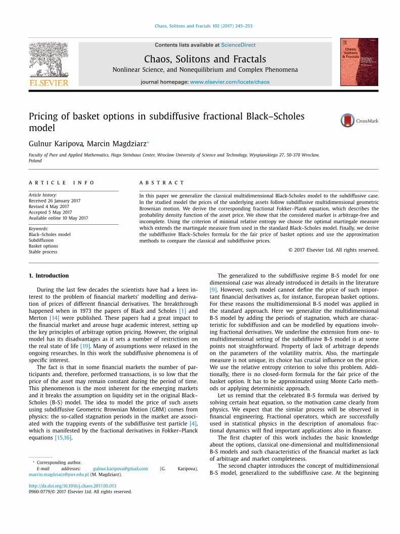
In Fig. 2 we compare trajectory of the first coordinate of stan-
ard multidimensional GBM and trajectory of the first coordinate
f the corresponding subdiffusive multidimensional GBM.
.3. Subdiffusive B-S formula
The following theorems verify the existence of martingale mea-
ures for Z α( t ).
heorem 2. If C ( t ) is a linear combination of independent Brownian
otions, i.e. C(t) =
∑ n i =1 γi W
(i ) (t) , γi = const, ∀ i, then the subdiffu-
ion process A (t) = C(S α(t)) is a martingale. Moreover, the stochastic
xponential of A ( t ) defined as
(t) = exp
{λA (t ) − λ2
2
〈 A (t ) , A (t ) 〉 }
, λ � = 0
s also a martingale. Here < A ( t ), A ( t ) > is the quadratic variation of
( t ) .
For the proof see the Appendix .
Let us introduce constants { γ j } n j=1 as the solution of the follow-
ng system
− μi −1
2
n ∑
j=1
σ 2 i j =
n ∑
j=1
σi j γ j , i = 1 , . . . , m. (19)
G. Karipova, M. Magdziarz / Chaos, Solitons and Fractals 102 (2017) 245–253 249
Fig. 2. Trajectories of Z (1) t and Z (1)
α (t) . Here, the parameters are: α = 0 . 9 , T = 1 , m = n = 10 , Z (i ) 0
= 1 , μi ∈ [ −2 , 3] , σ ij ∈ [0, 0.6], ∀ i, j = 1 , . . . , 10 .
T
Q
w
∈
C
m
c
p
a
s
s
i
m
L
Q
T
s
P
ε
m
D
O
D
T
R
d
p
d
m
T
f
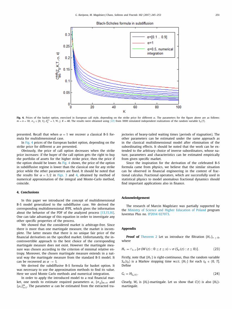
heorem 3. Let ε ≥ 0 . Let Q ε be the probability measure defined as
ε (A ) = C
∫ A
exp
{n ∑
i =1
γi W
(i ) (S α(T )) −(
ε +
1
2
n ∑
i =1
γ 2 i
)S α(T )
}dP,
(20)
here A ∈ F and C = [ E( exp { ∑ n i =1 γi W
(i ) (S α(T )) − (ε +1 2
∑ n i =1 γ
2 i ) S α(T ) } )] −1 is the normalizing constant. Then Z α( t ), t
[0, T ], is Q ε-martingale.
For the proof see the Appendix .
Two Fundamental Theorems of Asset Pricing imply that
orollary 1. The market model in which the asset prices follow the
ultidimensional subdiffusive GBM Z α( t ), has no arbitrage and is in-
omplete.
Market incompleteness means that there is no unique fair
rice of financial derivatives. Unfortunately, the incontrovertible
pproach to the best choice of the corresponding martingale mea-
ure does not exist. However the martingale measure can be cho-
en according to the criterion of minimal relative entropy, mean-
ng that the best choice of measure Q minimizes the distance from
easure P [10] .
emma 1. Let us define a probability measure Q as
(A ) =
∫ A
exp
{n ∑
i =1
γi W
(i ) (S α(T )) − 1
2
n ∑
i =1
γ 2 i S α(T )
}dP, A ∈ F .
(21)
hen the relative entropy for the measure Q is less than for the mea-
ure Q ε , ε > 0 .
roof. Clearly, Q is the special case of Q ε , defined in (20) for
= 0 and C = 1 . Thus, from Theorem 2 we have that Z α( t ) is a Q -
artingale.
The relative entropy of Q is equal to
= −∫ �
log dQ
dP dP =
1
2
E(S α(T )) n ∑
i =1
γ 2 i .
n the other hand, the relative entropy of Q ε is equal to
ε = −∫ �
log dQ ε
dP dP
= log E
(exp
{n ∑
i =1
γi W
(i ) (S α(T )) −(
ε +
1
2
n ∑
i =1
γ 2 i
)S α(T )
})
+
(
ε +
1
2
n ∑
i =1
γ 2 i
)
E(S α(T ))
= log E
(E
(exp
{n ∑
i =1
γi W
(i ) (S α(T )) − 1
2
n ∑
i =1
γ 2 i S α(T )
}
× exp {−εS α(T ) }| G t
))+
(ε +
1
2
n ∑
i =1
γ 2 i
)E(S α(T ))
= log E ( exp {−εS α(T ) } E (Y (t))) +
(ε +
1
2
n ∑
i =1
γ 2 i
)E(S α(T ))
= log E( exp {−εS α(T ) } ) +
(ε +
1
2
n ∑
i =1
γ 2 i
)E(S α(T ))
≥ 1
2
E(S α(T )) n ∑
i =1
γ 2 i = D.
hus, Q minimizes relative entropy. �
emark 1. Note that for α = 1 the measure Q defined in (21) re-
uces to the martingale measure in the standard B-S model.
Under the above arguments, further on we will find the fair
rices using the martingale measure Q . In the next theorem we
etermine the fair price of a basket option in the subdiffusive B-S
odel.
heorem 4. Let the assets prices follow Z α( t ) . Then the corresponding
air price C sub B −S
(Z 0 , K, T , σ, α) of a basket option satisfies

250 G. Karipova, M. Magdziarz / Chaos, Solitons and Fractals 102 (2017) 245–253
Fig. 3. Prices of the basket option, exercised in European call style, depending on the maturity time for different α. The parameters for the figure above are as follows:
m = n = 10 , σ ij ∈ [0, 1], Z (i ) 0
= 1 , ∀ i, j, K = 40 . The results were obtained using (22) from 10 0 0 simulated independent realizations of the random variable S α ( T ).
C
C
t
t
n
u
t
m
B
C
T
P
R
t
a
m
t
g
T
S
a
t
t
(
b
s
o
w
t
a
m
c
sub B −S (Z 0 , K, T , σ, α) = E(C B −S (Z 0 , K, S α(T ) , σ ))
=
∫ ∞
0
C B −S (Z 0 , K, x, σ ) T −αg α(x/T α) dx, (22)
where C B −S (Z 0 , K, T , σ ) is price of the basket option in the standard
multidimensional B-S model, g α( z ) stands for the PDF of S α(1) and
can be expressed using Fox function
g α(z) = H
10 11
(z| (1 −α,α)
(0 , 1)
).
Proof. The arbitrage-free rule of pricing requires that
sub B −S (Z 0 , K, T , σ, α) = E Q
((m ∑
i =1
ω i Z (i ) α (T ) − K
)+
)
= E
(exp
{n ∑
i =1
γi W
(i ) (S α(T ))
− 1
2
n ∑
i =1
γ 2 i S α(T )
}(m ∑
i =1
ω i Z (i ) α (T ) − K
)+
)
= E
(E
(exp
{n ∑
i =1
γi W
(i ) (S α(T ))
− 1
2
n ∑
i =1
γ 2 i S α(T )
}
×(
m ∑
i =1
ω i Z (i ) α (T ) − K
)+
)| S α(T )
)= E(C B −S (Z 0 , K, S α(T ) , σ ))
=
∫ ∞
0
C B −S (Z 0 , K, x, σ ) g α(x, T ) dx.
Here by g α( x, T ) we denote the PDF of S α( T ). since S α( T ) is α-
selfsimilar, we obtain g α(x, T ) = T −αg α(x/T α) . Thus, the statement
follows. �
Remark 2. There is no explicit formula for C B −S (Z 0 , K, T , σ ) , there-
fore, in order to find the basket option price in the subdiffusive
case, it is necessary to use the approximation methods. One needs
o approximate first the classical price C B −S (Z 0 , K, x, σ ) using Gen-
le’s approximation (already given in (8) , see [6,17] ). Next, one
eeds to approximate the integral ∫ ∞
0 C B −S (Z 0 , K, x, σ ) g α(x, T ) dx
sing some standard method. Another possibility is to use the fact
hat C sub B −S
(Z 0 , K, T , σ, α) = E(C B −S (Z 0 , K, S α(T ) , σ )) and to approxi-
ate C sub B −S
(Z 0 , K, T , σ, α) using Monte Carlo methods.
The put-call parity applied to the multidimensional subdiffusive
-S model, with r = 0 is as follows
sub B −S (Z 0 , K, T , σ, α) − P sub
B −S (Z 0 , K, T , σ, α) = Z α(0) − K, .
hus the subdiffusive price of the put option yields
sub B −S (Z 0 , K, T , σ, α) = C sub
B −S (Z 0 , K, T , σ, α) + K − Z α(0) .
emark 3. The derivatives prices with payoff functions, different
han European basket option, can be calculated using analogous
pproach.
The above result allows us to find fair price of basket option in
ultidimensional subdiffusive B-S model. For instance, for α = 1 / 2
he Fox function can be evaluated as follows [18]
1 / 2 (z) =
1 √
πexp
{− z 2
4
}, z ≥ 0 .
he price of a basket option in the classical Multidimensional B-
model can be found using Gentle’s approximation by geometric
verage, mentioned in previous chapter. The approximate value of
he classical B-S formula is given by (8) . Thus, one can estimate
he value of C sub B −S
by numerical integration of expression in formula
22) . Another method of finding the price of the basket option is
y using well-known Monte Carlo methods. It is only needed to
imulate the realization of S α( T ). From the self-similarity property
f S α( t ) it is evident that S α( T ) is equal in distribution to (
T U α (1)
)α,
here U α( τ ) is α-stable subordinator. U α(1) can be generated in
he standard way, see [5] . Thus, one only needs to simulate U α(1)
nd estimate the expectations in formula (22) using Monte-Carlo
ethod.
In Fig. 3 prices of the basket option, exercised in European
all style, depending on the maturity time for different α are
G. Karipova, M. Magdziarz / Chaos, Solitons and Fractals 102 (2017) 245–253 251
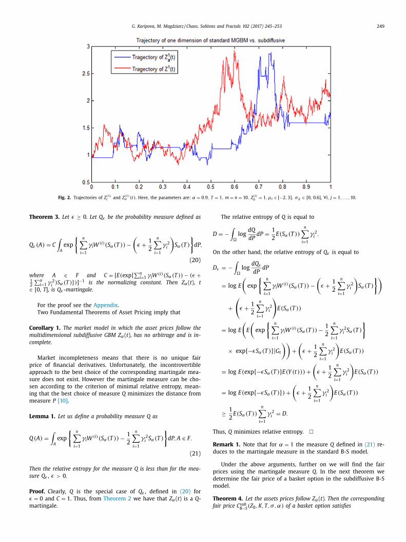
Fig. 4. Prices of the basket option, exercised in European call style, depending on the strike price for different α. The parameters for the figure above are as follows:
m = n = 10 , σ ij ∈ [0, 1], Z (i ) 0
= 1 , ∀ i, j, K = 40 . The results were obtained using (22) from 10 0 0 simulated independent realizations of the random variable S α( T ).
p
m
s
p
t
t
i
p
t
n
c
4
B
c
a
O
o
t
p
fi
c
m
s
t
u
c
w
H
k
{
j
o
i
s
t
t
f
f
c
t
s
fi
A
t
I
A
w
H
F
S
D
G
C
m
resented. Recall that when α = 1 we recover a classical B-S for-
ula for multidimensional case.
In Fig. 4 prices of the European basket option, depending on the
trike price for different α are presented.
Obviously, the price of call option decreases when the strike
rice increases: if the buyer of the call option gets the right to buy
he portfolio of assets for the higher strike price, then the price if
he option should be lower. As Fig. 4 shows, the price of the option
n subdiffusive regime is lower than the classical one for any strike
rice while the other parameters are fixed. It should be noted that
he results for α = 1 / 2 in Figs. 3 and 4 , obtained by method of
umerical approximation of the integral and Monte-Carlo method,
oincide.
. Conclusions
In this paper we introduced the concept of multidimensional
-S model generalized to the subdiffusive case. We derived the
orresponding multidimensional fFPE, which gives the information
bout the behavior of the PDF of the analyzed process [13,15,16] .
ne can take advantage of this equation in order to investigate any
ther specific properties of the process.
We showed that the considered market is arbitrage-free. Since
here is more than one martingale measure, the market is incom-
lete. The latter means that there is no unique fair price of the
nancial derivatives on the specified market. Unfortunately, the in-
ontrovertible approach to the best choice of the corresponding
artingale measure does not exist. However the martingale mea-
ure was chosen according to the criterion of minimal relative en-
ropy. Moreover, the chosen martingale measure extends in a nat-
ral way the martingale measure from the standard B-S model. It
an be recovered as α → 1.
We derived the subdiffusive B-S formula for basket option. It
as necessary to use the approximation methods to find its value.
ere we used Monte Carlo methods and numerical integration.
In order to apply the introduced model to a real financial mar-
et, one needs to estimate required parameters α, { σ ij } m ×n and
μi } m
i =1 . The parameter α can be estimated from the extracted tra-
ectories of heavy-tailed waiting times (periods of stagnation). The
ther parameters can be estimated under the same approach as
n the classical multidimensional model after elimination of the
ubordinating effects. It should be noted that the work can be ex-
ended to the arbitrary choice of inverse subordinators, whose na-
ure, parameters and characteristics can be estimated empirically
rom given specific market.
Since the inspiration for the derivation of the celebrated B-S
ormula came from physics, we believe that the similar situation
an be observed in financial engineering in the context of frac-
ional calculus. Fractional operators, which are successfully used in
tatistical physics to model anomalous fractional dynamics should
nd important applications also in finance.
cknowledgement
The research of Marcin Magdziarz was partially supported by
he Ministry of Science and Higher Education of Poland program
uventus Plus no. IP2014 027073 .
ppendix
Proof of Theorem 2 Let us introduce the filtration { H τ } τ ≥ 0 ,
here
τ = ∩ s>τ { σ (W (z) : 0 ≤ z ≤ s ) ∨ σ (S α(z) : z ≥ 0) } . (23)
irstly, note that { H τ } is right-continuous, thus the random variable
α( t 0 ) is a Markov stopping time w.r.t. { H τ } for each t 0 ∈ (0, T ].
efine
t = H S α (t) . (24)
learly, W t is { H t }-martingale. Let us show that C ( t ) is also { H t }-
artingale.
252 G. Karipova, M. Magdziarz / Chaos, Solitons and Fractals 102 (2017) 245–253
Y
Y
Y
a
h
Q
T
o
E
U
E
f
E
A
m
i
E
T
E
T
f
t
Z
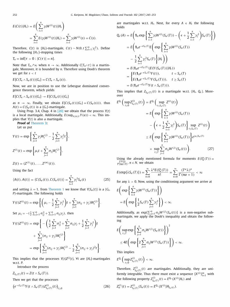
E(C(t) | H s ) = E
(n ∑
i =1
γi W
(i ) (t) | H s
)
=
n ∑
i =1
E(γi W
(i ) (t) | H s ) =
n ∑
i =1
γi W
(i ) (s ) = C(s ) .
Therefore, C ( t ) is { H t }-martingale, C(t) ∼ N(0 , t ∑ n
i =1 γ2
i ) . Define
the following { H τ }-stopping times
T n = inf { τ > 0 : | C(τ ) | = n } . Note that T n ↗∞ when n → ∞ . Additionally C ( T n ∧ τ ) is a martin-
gale, Moreover, it is bounded by n . Therefore using Doob’s theorem
we get for s < t
E{ C(T n ∧ S α(t)) | G s } = C(T n ∧ S α(s )) .
Now, we are in position to use the Lebesgue dominated conver-
gence theorem, which yields
E{ C(T n ∧ S α(t)) | G s } → E{ C(S α(t)) | G s } as n → ∞ . Finally, we obtain E{ C(S α(t)) | G s } = C(S α(s ))) , thus
A (t) = C(S α(t)) is a { G t }-martingale.
Using Prop. 3.4, Chap. 4 in [20] we obtain that the process Y ( t )
is a local martingale. Additionally, E( sup o≤u ≤t Y (u )) < ∞ . This im-
plies that Y ( t ) is also a martingale.
Proof of Theorem 3 :
Let us put
(t) = exp
{n ∑
j=1
γ j W
( j) t − 1
2
n ∑
j=1
γ 2 j t
},
Z (i ) (t) = exp
{μi t +
n ∑
j=1
σi j W
( j) t
},
Z(t) = (Z (1) (t ) , . . . , Z (m ) (t )) .
Using the fact
〈 A (t) , A (t) 〉 = 〈 C(S α(t)) , C(S α(t)) 〉 =
n ∑
i =1
γ 2 i S α(t) (25)
and setting λ = 1 , from Theorem 1 we know that Y ( S α( t )) is a ( G t ,
P )-martingale. The following holds
(t) Z (i ) (t) = exp
{(μi −
1
2
n ∑
j=1
γ 2 j
)t +
n ∑
j=1
(σi j + γ j ) W
( j) t
}.
Set μi = −( 1 2
∑ n j=1 σ
2 i j
+
∑ n j=1 σi j γ j ) , then
(t) Z (i ) (t) = exp
{−
(1
2
n ∑
j=1
σ 2 i j +
n ∑
j=1
σi j γ j +
1
2
n ∑
j=1
γ 2 j
)t
+
n ∑
j=1
(σi j + γ j ) W
( j) t
}
= exp
{n ∑
j=1
(σi j + γ j ) W
( j) t − 1
2
n ∑
j=1
(σi j + γ j ) 2 t
}.
This implies that the processes Y ( t ) Z ( i ) ( t ), ∀ i are { H t }-martingales
w.r.t. P .
Introduce the process
Z S α (T ) (t) = Z(t ∧ S α(T )) .
Then we get that the processes (e −εS α (T ) Y (t ∧ S α(T )) Z (i )
S α (T ) (t)
)t≥0
(26)
re martingales w.r.t. H t . Next, for every A ∈ H t the following
olds
ε (A ) = E
(1 A exp
{n ∑
i =1
γi W
(i ) (S α(T )) −(
ε +
1
2
n ∑
i =1
γ 2 i
)S α(T )
})
= E
(1 A e
−εS α (T ) E
(exp
{n ∑
i =1
γi W
(i ) (S α(T ))
− 1
2
n ∑
i =1
γ 2 i S α(T )
}| H t
))= E ( 1 A e
−εS α (T ) (E (Y (S α(T )) | H t ))
=
{E( 1 A e
−εS α (T ) Y (t)) , t < S α(T )
E( 1 A e −εS α (T ) Y (S α(T ))) , t ≥ S α(T )
= E( 1 A e −εS α (T ) Y (t ∧ S α(T ))) .
his implies that Z S α(T ) (t) is a martingale w.r.t. ( H t , Q ε ). More-
ver
Q ε
(sup
t≥0
Z (i ) S α (T )
(t) )
= E Q ε(
sup
t≤S α (T )
Z (i ) (t) )
= E
(exp
{n ∑
i =1
γi W
(i ) (S α(T ))
−(
ε +
1
2
n ∑
i =1
γ 2 i
)S α(T )
}sup
t≤S α (T )
Z (i ) (t)
)
≤ E
(exp
{n ∑
i =1
γi W
(i ) (S α(T ))
}e | μi | S α (T )
× sup
t≤T
n ∑
j=1
σi j W
( j) (S α(t))
). (27)
sing the already mentioned formula for moments E(S n α(T )) =T nαn !
(nα+1) , n ∈ N, we obtain
( exp { λS α(T ) } ) =
∞ ∑
n =0
λn E(S n α(T ))
n ! =
∞ ∑
n =0
(T αλ) n
(nα + 1) < ∞
or any λ > 0. Now, using the conditioning argument we arrive at
(exp
{n ∑
i =1
γi W
(i ) (S α(T ))
})
= E
(exp
{1
2
S α(T ) n ∑
j=1
γ 2 j
})< ∞ .
dditionally, as exp { ∑ n j=1 σi j W
( j) (S α(t)) } is a non-negative sub-
artingale, we apply the Doob’s inequality and obtain the follow-
ng
(sup
t≤T
exp
{n ∑
j=1
σi j W
( j) (S α(t))
})2
≤ 4 E
(exp
{2
n ∑
j=1
σi j W
( j) (S α(T ))
})< ∞ .
his implies
Q ε
(sup
t≥0
Z (i ) S α (T )
(t) )
< ∞ .
herefore, Z (i ) S α(T )
(t) are martingales. Additionally, they are uni-
ormly integrable. Thus there must exist a sequence { X (i ) } m
i =1 with
he following property Z (i ) S α(T )
(t) = E Q ε (X (i ) | H t ) and
(i ) α (t) = Z (i )
S α (T ) (S α(t)) = E Q ε (X
(i ) | H S α (t) ) .

G. Karipova, M. Magdziarz / Chaos, Solitons and Fractals 102 (2017) 245–253 253
L
ε
m
R
[
[
[
astly, Z α( t ) is a martingale w.r.t. (H S α(t) , Q ε ) Note that for each
≥ > 0 we obtain different measure Q ε . So, there is no unique
artingale measure for Z α( t ). �
eferences
[1] Black F , Scholes M . The pricing of options and corporate liabilities. J Pol Econ1973;81:637–54 .
[2] Company R , Jodar L . Numerical solution of Black–Scholes option pricing with
variable yield discrete dividend payment. Banach Cent Publ 2008;83:37–47 . [3] Cont R , Tankov P . Financial modeling with jump processes. Chapman &
Hall/CRC, Boca Raton; 2004 . [4] Elizar I , Klafler J . Spatial gliding, temporal trapping and anomalous transport.
Physica D 2004;187:30–50 . [5] Janicki A , Weron A . Simulation and chaotic behaviour of α-stable stochastic
processes. New York: Marcel Dekker; 1994 .
[6] Krekel M , Kock J , Korn R , Man T-K . An analysis of pricing methods for basketsoptions. Wilmott Mag 2004;3:82–9 .
[7] Li GH , Zhang H , Luo MK . A multidimensional subdiffusion model: an arbi-trage-free market. Chin Phys B 2012;21:128901 .
[8] Magdziarz M , Weron A . Anomalous diffusion and semimartingales. EPL20 09;86:60 010 .
[9] Magdziarz M . Black–Scholes formula in subdiffusive regime. J Stat Phys
2009;136:553–64 . [10] Magdziarz M , Gajda J . Anomalous dynamics of Black–Scholes model time
changed by inverse subordinators. ACTA Physica Polonica 2012;B 43:1093–110 .[11] Magdziarz M . Path properties of subdiffusion - a martingale approach. Stochas-
tic Models 2010;26:256–71 .
[12] Magdziarz M . Stochastic representation of subdiffusion processes withtime-dependent drift. Stochastic Process Appl 2009;119:3238–52 .
[13] Martens W , Wagner U . Advances in solving high dimensional Fokker–Planckequations. Rome: ENOC; 2011 .
[14] Merton RC . Theory of rational option pricing. Bell J Econ Manag Sci1973;4:141–83 .
[15] Metzler R , Barkai E , Klafter J . Anomalous diffusion and relaxation close to ther-mal equilibrium: a fractional Fokker–Planck equation approach. Phys Rev Lett
1999;82:3563–7 .
[16] Metzler R , Klafter J . The random walk’s guide to anomalous diffusion: a frac-tional dynamics approach. Phys Rep 20 0 0;339:1–77 .
[17] Musiela M , Rutkowski M . Martingale methods in financial modelling. Berlin:Springer; 1997 .
[18] Piryatinska A , Saichev AI , Woyczynski WA . Models of anomalous diffusion: thesubdiffusive case. Physica 2005;A 349:375–420 .
[19] Ray S . A close look into Black–Scholes option pricing model. J Sci (JOS)
2012;2:172–8 . 20] Revuz D , Yor M . Continuous martingales and Brownian motion. Berlin:
Springer; 1999 . [21] Samko SG , Kilbas AA , Maritchev DI . Integrals and derivatives of the fractional
order and some of their applications. Amsterdam: Gordon and Breach; 1993 . 22] Xu L . Ergodicity of the stochastic real Ginzburg–Landau equation driven by
α-stable noises. Stochastic Process Appl 2013;123:3710–36 .
23] Zhang X . Derivative formulas and gradient estimates for SDEs driven byα-stable processes. Stochastic Process Appl 2013;123:1213–28 .

本文献由“学霸图书馆-文献云下载”收集自网络,仅供学习交流使用。
学霸图书馆(www.xuebalib.com)是一个“整合众多图书馆数据库资源,
提供一站式文献检索和下载服务”的24 小时在线不限IP
图书馆。
图书馆致力于便利、促进学习与科研,提供最强文献下载服务。
图书馆导航:
图书馆首页 文献云下载 图书馆入口 外文数据库大全 疑难文献辅助工具


