

Chapter 34
Electromagnetic Waves

Modifications to Ampère’s Law
Ampère’s Law is used to analyze magnetic fields created by currents:
But this form is valid only if any electric fields present are constant in time
Maxwell modified the equation to include time-varying electric fields
Maxwell’s modification was to add a term
od μ IB s
Modifications to Ampère’s Law, cont
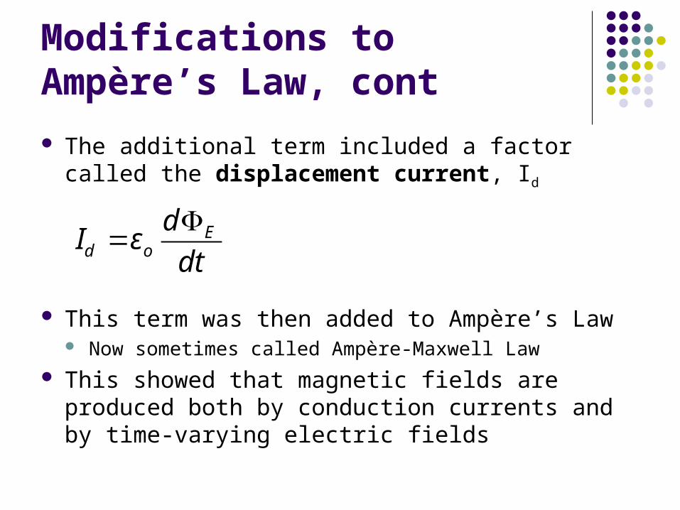
The additional term included a factor called the displacement current, Id
This term was then added to Ampère’s Law Now sometimes called Ampère-Maxwell Law
This showed that magnetic fields are produced both by conduction currents and by time-varying electric fields
Ed o
dI ε
dt
Maxwell’s Equations
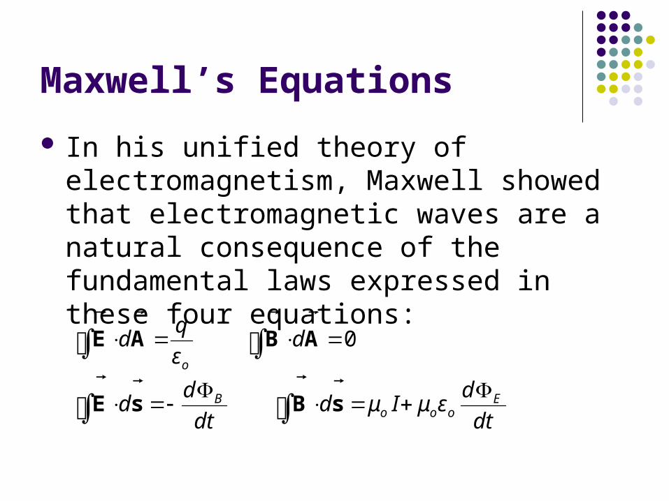
In his unified theory of electromagnetism, Maxwell showed that electromagnetic waves are a natural consequence of the fundamental laws expressed in these four equations:
0o
B Eo o o
qd d
ε
d dd d μ I μ ε
dt dt
E A B A
E s B s
Maxwell’s Equation 1 – Gauss’ Law
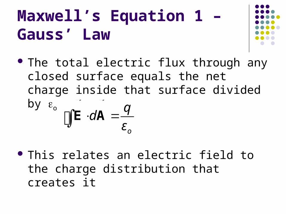
The total electric flux through any closed surface equals the net charge inside that surface divided by o
This relates an electric field to the charge distribution that creates it
o
qd
ε E A
Maxwell’s Equation 2 – Gauss’ Law in Magnetism
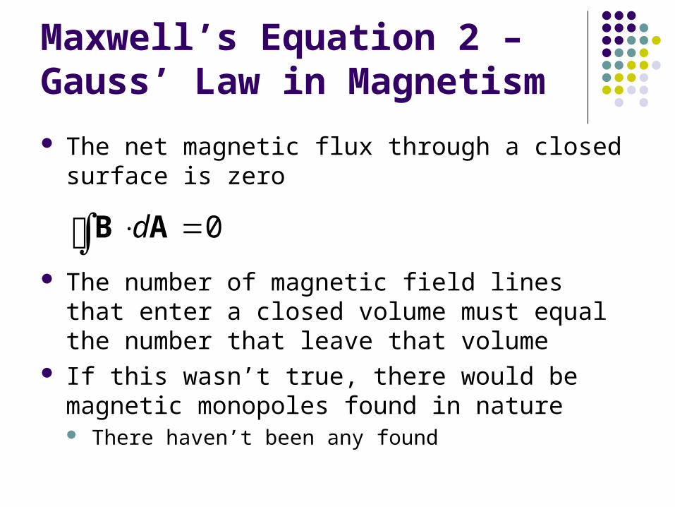
The net magnetic flux through a closed surface is zero
The number of magnetic field lines that enter a closed volume must equal the number that leave that volume
If this wasn’t true, there would be magnetic monopoles found in nature There haven’t been any found
0d B A
Maxwell’s Equation 3 – Faraday’s Law of Induction
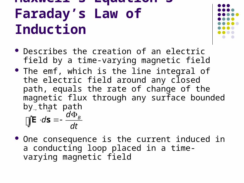
Describes the creation of an electric field by a time-varying magnetic field
The emf, which is the line integral of the electric field around any closed path, equals the rate of change of the magnetic flux through any surface bounded by that path
One consequence is the current induced in a conducting loop placed in a time-varying magnetic field
Bdd
dt
E s

Maxwell’s Equation 4 – Ampère-Maxwell Law
Describes the creation of a magnetic field by a changing electric field and by electric current
The line integral of the magnetic field around any closed path is the sum of o times the net current through that path and o times the rate of change of electric flux through any surface bounded by that path
Eo o o
dd μ I ε μ
dt
B s
Lorentz Force Law
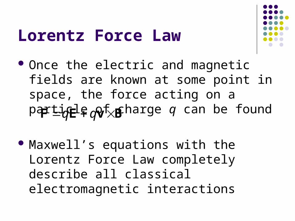
Once the electric and magnetic fields are known at some point in space, the force acting on a particle of charge q can be found
Maxwell’s equations with the Lorentz Force Law completely describe all classical electromagnetic interactions
q q F E v B
Speed of Electromagnetic Waves
In empty space, q = 0 and I = 0 The last two equations can be solved to show
that the speed at which electromagnetic waves travel is the speed of light
This result led Maxwell to predict that light waves were a form of electromagnetic radiation

Plane em Waves
We will assume that the vectors for the electric and magnetic fields in an em wave have a specific space-time behavior that is consistent with Maxwell’s equations
Assume an em wave that travels in the x direction with
as shown
andE B
PLAYACTIVE FIGURE
Plane em Waves, cont.
The x-direction is the direction of propagation The electric field is assumed to be in the y direction
and the magnetic field in the z direction Waves in which the electric and magnetic fields are
restricted to being parallel to a pair of perpendicular axes are said to be linearly polarized waves
We also assume that at any point in space, the magnitudes E and B of the fields depend upon x and t only
Rays
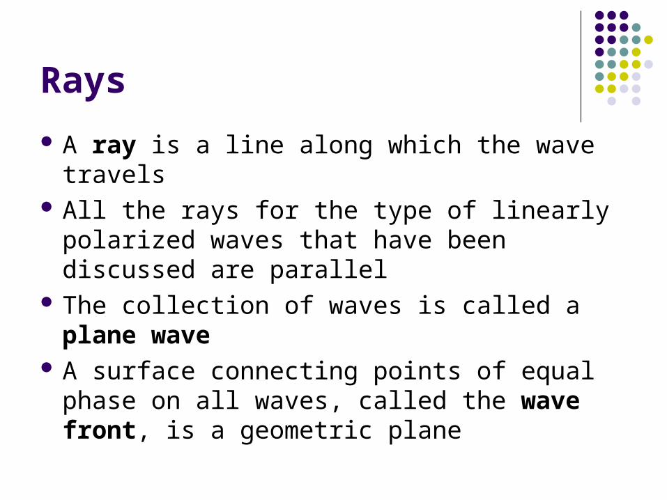
A ray is a line along which the wave travels All the rays for the type of linearly polarized
waves that have been discussed are parallel The collection of waves is called a plane
wave A surface connecting points of equal phase
on all waves, called the wave front, is a geometric plane

Wave Propagation, Example
The figure represents a sinusoidal em wave moving in the x direction with a speed c
Use the active figure to observe the motion
Take a “snapshot” of the wave and investigate the fields
PLAYACTIVE FIGURE

Waves – A Terminology Note
The word wave represents both The emission from a single point The collection of waves from all points on the
source The meaning should be clear from the
context

Properties of em Waves
The solutions of Maxwell’s third and fourth equations are wave-like, with both E and B satisfying a wave equation
Electromagnetic waves travel at the speed of light:
This comes from the solution of Maxwell’s equations
1
o o
cμ ε
Properties of em Waves, 2
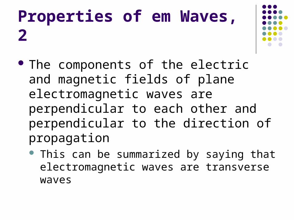
The components of the electric and magnetic fields of plane electromagnetic waves are perpendicular to each other and perpendicular to the direction of propagation This can be summarized by saying that
electromagnetic waves are transverse waves
Properties of em Waves, 3
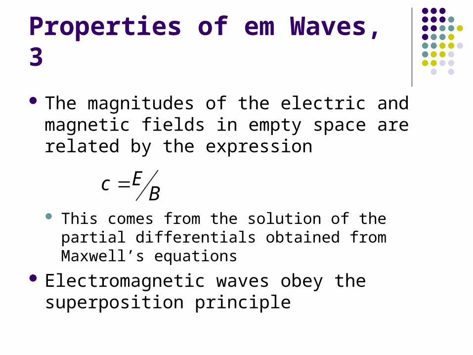
The magnitudes of the electric and magnetic fields in empty space are related by the expression
This comes from the solution of the partial differentials obtained from Maxwell’s equations
Electromagnetic waves obey the superposition principle
Ec B

Derivation of Speed – Some Details
From Maxwell’s equations applied to empty space, the following partial derivatives can be found:
These are in the form of a general wave equation, with
Substituting the values for μo and εo gives c = 2.99792 x 10⁸ m/s
2 2 2 2
2 2 2 2o o o o
E E B Bμ ε and μ ε
x t x t
1
o o
v cμ ε

E to B Ratio – Some Details
The simplest solution to the partial differential equations is a sinusoidal wave: E = Emax cos (kx – ωt)
B = Bmax cos (kx – ωt)
The angular wave number is k = 2π/λ λ is the wavelength
The angular frequency is ω = 2πƒ ƒ is the wave frequency
E to B Ratio – Details, cont.
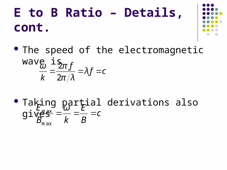
The speed of the electromagnetic wave is
Taking partial derivations also gives
2
2
ƒƒ
ω πλ c
k π λ
max
max
E ω Ec
B k B
Poynting Vector
Electromagnetic waves carry energy As they propagate through space, they can
transfer that energy to objects in their path The rate of flow of energy in an em wave is
described by a vector, , called the Poynting vector
S

Poynting Vector, cont.
The Poynting vector is defined as
Its direction is the direction of propagation
This is time dependent Its magnitude varies in time Its magnitude reaches a
maximum at the same instant as
1
oμ S E B
andE B

Poynting Vector, final
The magnitude of represents the rate at which energy flows through a unit surface area perpendicular to the direction of the wave propagation This is the power per unit area
The SI units of the Poynting vector are J/(s.m2) = W/m2
S
Intensity
The wave intensity, I, is the time average of S (the Poynting vector) over one or more cycles
When the average is taken, the time average of cos2(kx - ωt) = ½ is involved
2 2max max max max
avg 2 2 2o o o
E B E c BI S
μ μ c μ
Energy Density
The energy density, u, is the energy per unit volume
For the electric field, uE= ½ εoE2
For the magnetic field, uB = ½ μoB2
Since B = E/c and 1 o oc μ ε
221
2 2B E oo
Bu u ε E
μ
Energy Density, cont.
The instantaneous energy density associated with the magnetic field of an em wave equals the instantaneous energy density associated with the electric field In a given volume, the energy is shared equally
by the two fields

Energy Density, final
The total instantaneous energy density is the sum of the energy densities associated with each field u =uE + uB = εoE2 = B2 / μo
When this is averaged over one or more cycles, the total average becomes uavg = εo(E2)avg = ½ εoE2
max = B2max / 2μo
In terms of I, I = Savg = cuavg The intensity of an em wave equals the average
energy density multiplied by the speed of light

Momentum
Electromagnetic waves transport momentum as well as energy
As this momentum is absorbed by some surface, pressure is exerted on the surface
Assuming the wave transports a total energy TER to the surface in a time interval Δt, the total momentum is p = TER / c for complete absorption
Pressure and Momentum
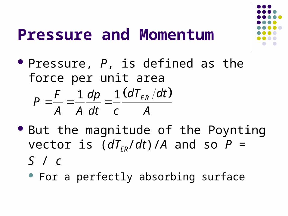
Pressure, P, is defined as the force per unit area
But the magnitude of the Poynting vector is (dTER/dt)/A and so P = S / c For a perfectly absorbing surface
1 1 ERdT dtF dpP
A A dt c A

Pressure and Momentum, cont.
For a perfectly reflecting surface,
p = 2TER /c and P = 2S/c For a surface with a reflectivity somewhere
between a perfect reflector and a perfect absorber, the pressure delivered to the surface will be somewhere in between S/c and 2S/c
For direct sunlight, the radiation pressure is about 5 x 10⁻⁶ N/m2

Production of em Waves by an Antenna
Neither stationary charges nor steady currents can produce electromagnetic waves
The fundamental mechanism responsible for this radiation is the acceleration of a charged particle
Whenever a charged particle accelerates, it radiates energy
Production of em Waves by an Antenna, 2
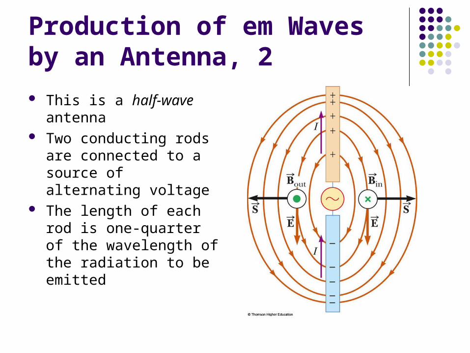
This is a half-wave antenna Two conducting rods are
connected to a source of alternating voltage
The length of each rod is one-quarter of the wavelength of the radiation to be emitted

Production of em Waves by an Antenna, 3
The oscillator forces the charges to accelerate between the two rods
The antenna can be approximated by an oscillating electric dipole
The magnetic field lines form concentric circles around the antenna and are perpendicular to the electric field lines at all points
The electric and magnetic fields are 90o out of phase at all times
This dipole energy dies out quickly as you move away from the antenna

Production of em Waves by an Antenna, final
The source of the radiation found far from the antenna is the continuous induction of an electric field by the time-varying magnetic field and the induction of a magnetic field by a time-varying electric field
The electric and magnetic field produced in this manner are in phase with each other and vary as 1/r
The result is the outward flow of energy at all times
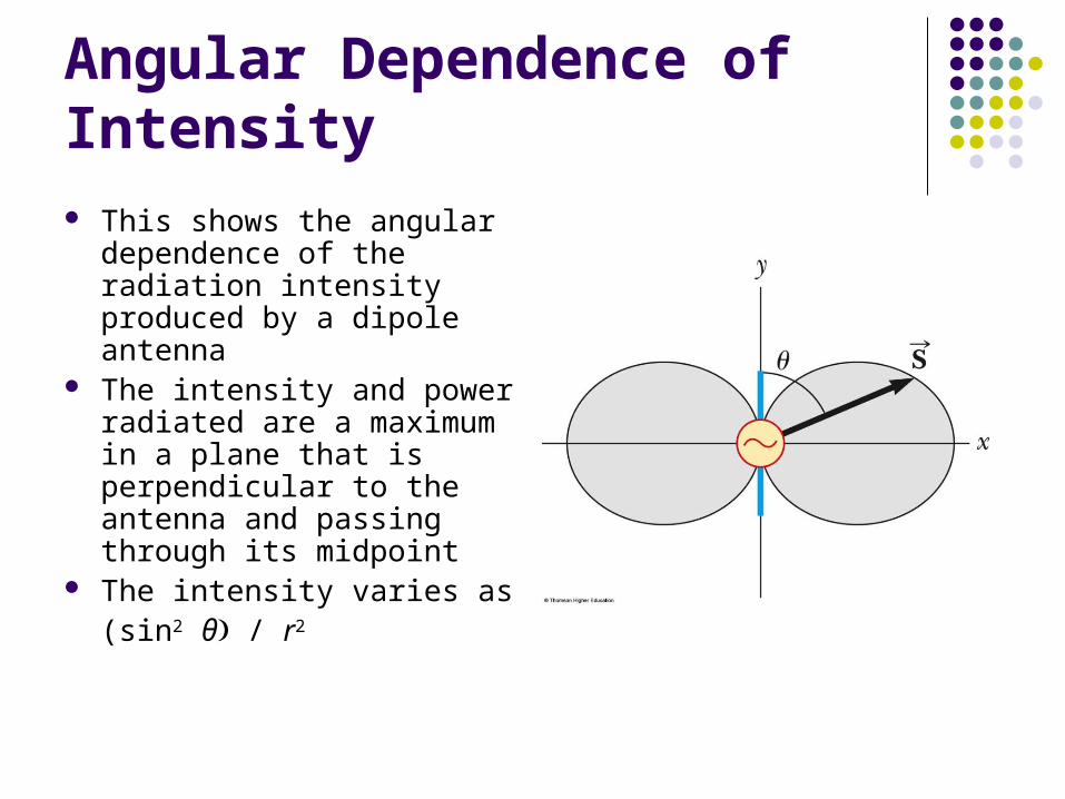
Angular Dependence of Intensity This shows the angular
dependence of the radiation intensity produced by a dipole antenna
The intensity and power radiated are a maximum in a plane that is perpendicular to the antenna and passing through its midpoint
The intensity varies as (sin2 θ / r2

The Spectrum of EM Waves
Various types of electromagnetic waves make up the em spectrum
There is no sharp division between one kind of em wave and the next
All forms of the various types of radiation are produced by the same phenomenon – accelerating charges
The EM Spectrum
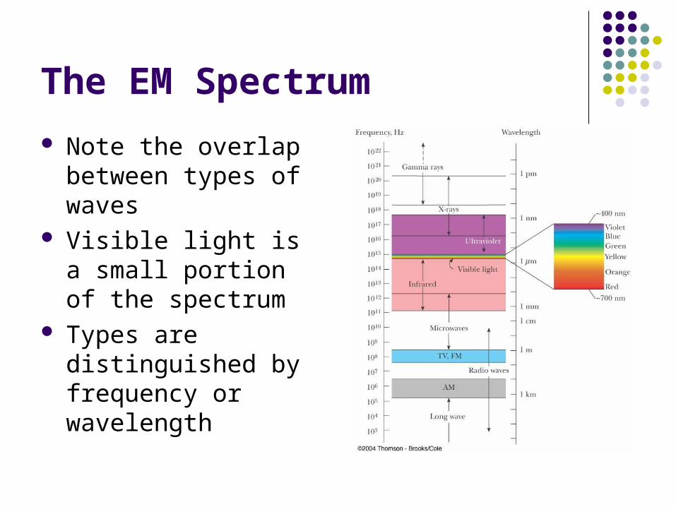
Note the overlap between types of waves
Visible light is a small portion of the spectrum
Types are distinguished by frequency or wavelength
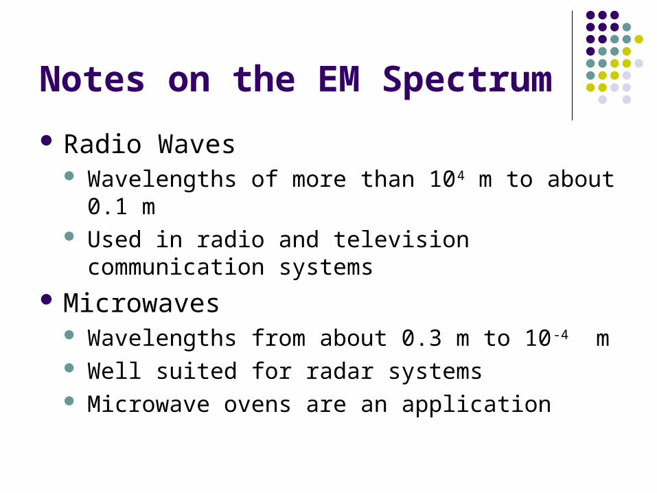
Notes on the EM Spectrum
Radio Waves Wavelengths of more than 104 m to about 0.1 m Used in radio and television communication
systems Microwaves
Wavelengths from about 0.3 m to 10-4 m Well suited for radar systems Microwave ovens are an application
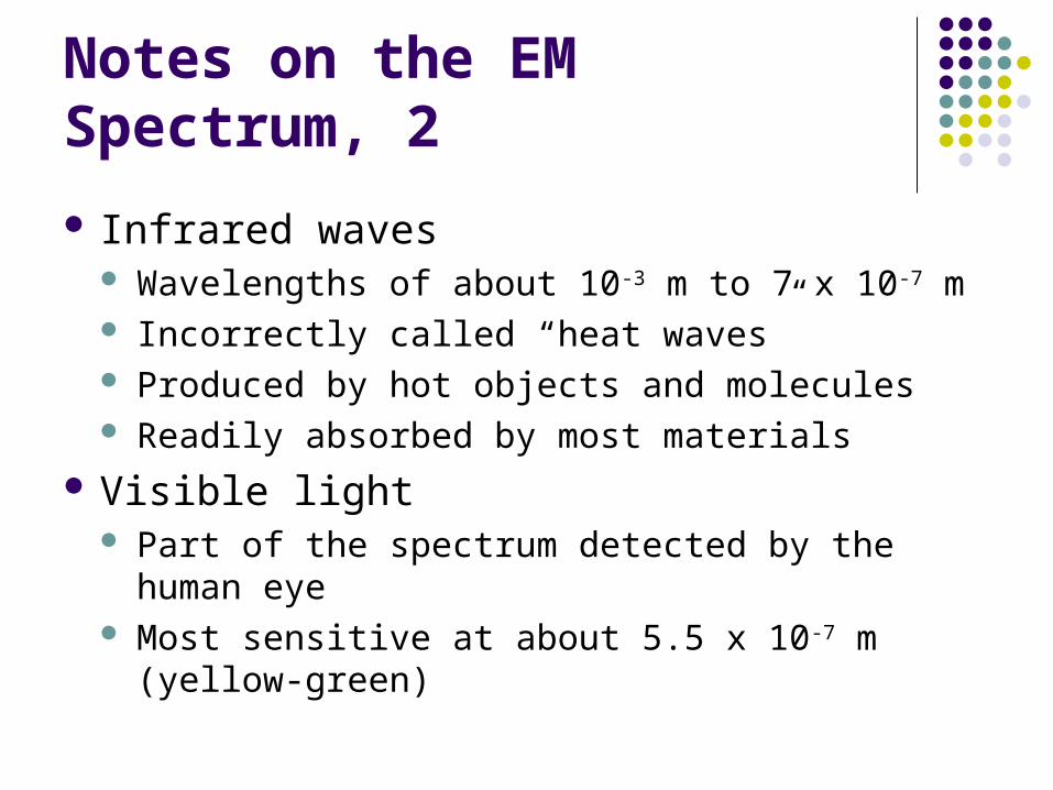
Notes on the EM Spectrum, 2
Infrared waves Wavelengths of about 10-3 m to 7 x 10⁻⁷ m Incorrectly called “heat waves” Produced by hot objects and molecules Readily absorbed by most materials
Visible light Part of the spectrum detected by the human eye Most sensitive at about 5.5 x 10⁻⁷ m (yellow-
green)

More About Visible Light
Different wavelengths correspond to different colors
The range is from red (λ ~ 7 x 10⁻⁷ m) to violet (λ ~4 x 10⁻⁷ m)
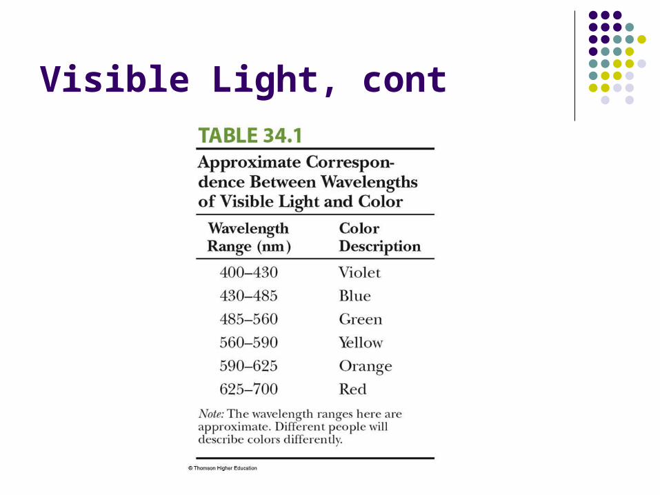
Visible Light, cont
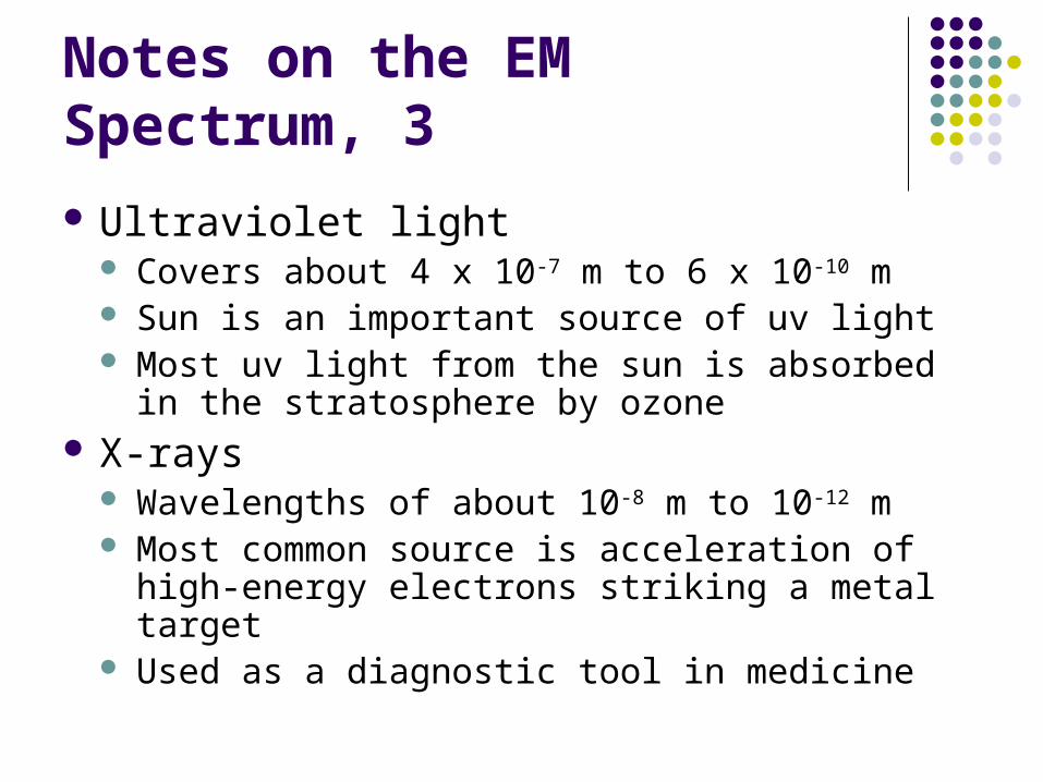
Notes on the EM Spectrum, 3
Ultraviolet light Covers about 4 x 10⁻⁷ m to 6 x 10⁻¹⁰ m Sun is an important source of uv light Most uv light from the sun is absorbed in the
stratosphere by ozone X-rays
Wavelengths of about 10-8 m to 10-12 m Most common source is acceleration of high-
energy electrons striking a metal target Used as a diagnostic tool in medicine
Notes on the EM Spectrum, final
Gamma rays Wavelengths of about 10-10 m to 10-14 m Emitted by radioactive nuclei Highly penetrating and cause serious damage
when absorbed by living tissue Looking at objects in different portions of the
spectrum can produce different information
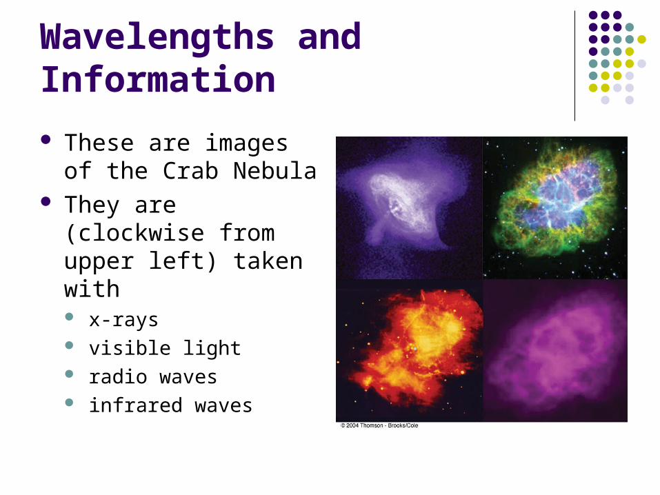
Wavelengths and Information
These are images of the Crab Nebula
They are (clockwise from upper left) taken with x-rays visible light radio waves infrared waves


![L 28 Electricity and Magnetism [6] magnetism Faraday’s Law of Electromagnetic Induction –induced currents –electric generator –eddy currents Electromagnetic.](https://static.documents.pub/doc/80x56/56649d035503460f949d6537/l-28-electricity-and-magnetism-6-magnetism-faradays-law-of-electromagnetic.jpg)
