

Chapter 6
Finite Differences
6.1 Introduction
For a function 𝑦 = 𝑓 𝑥 , finite differences refer to
changes in values of 𝑦 (dependent variable) for any
finite (equal or unequal) variation in 𝑥 (independent
variable).
In this chapter, we shall study various differencing
techniques for equal deviations in values of 𝑥 and
associated differencing operators; also their
applications will be extended for finding missing
values of a data and series summation.
6.2 Shift or Increment Operator (𝑬)
Shift (Increment) operator denoted by ‘𝐸’ operates on 𝑓(𝑥) as 𝐸𝑓 𝑥 = 𝑓 𝑥 +
Or 𝐸𝑦𝑥 = 𝑦𝑥+ , where ‘’ is the step height for equi-spaced data points.
Clearly effect of the shift operator 𝐸 is to shift the function value to the next
higher value 𝑓 𝑥 + or 𝑦𝑥+
Also 𝐸2𝑓 𝑥 = 𝐸 𝐸𝑓(𝑥) = 𝐸𝑓 𝑥 + = 𝑓 𝑥 + 2
∴ 𝐸𝑛𝑓 𝑥 = 𝑓 𝑥 + 𝑛
Moreover 𝐸−1𝑓 𝑥 = 𝑓 𝑥 − , where 𝐸−1 is the inverse shift operator.
6.3 Differencing Operators
If 𝑦0, 𝑦1, 𝑦2 , …𝑦𝑛 be the values of 𝑦 for corresponding values of 𝑥0, 𝑥1, 𝑥2 ,
…𝑥𝑛 , then the differences of 𝑦 are defined by (𝑦1 − 𝑦0), (𝑦2 − 𝑦1), … , (𝑦𝑛 − 𝑦𝑛−1) , and are denoted by different operators discussed in this section.
6.3.1 Forward Difference Operator ∆
Forward difference operator ‘∆’ operates on 𝑦𝑥 as ∆𝑦𝑥 = 𝑦𝑥+1− 𝑦𝑥
Or ∆𝑓 𝑥 = 𝑓 𝑥 + − 𝑓 𝑥 , where is the height of differencing.
∴ ∆𝑦0 = 𝑦1− 𝑦0
∆𝑦1 = 𝑦2− 𝑦1
⋮
∆𝑦𝑛 = 𝑦𝑛+1− 𝑦𝑛
Also ∆2𝑦0 = ∆𝑦1− ∆𝑦0 = 𝑦2− 𝑦1 − 𝑦1− 𝑦0 = 𝑦2 − 2𝑦1 + 𝑦0
⋮
∆𝑛𝑦0 = 𝑦𝑛 − 𝑛𝐶1𝑦𝑛−1 + 𝑛𝐶2𝑦𝑛−2 −⋯+ −1 𝑛−1 𝑛𝐶𝑛−1𝑦1 + −1 𝑛𝑦0
Generalizing ∆𝑛𝑦𝑟 = 𝑦𝑛+𝑟 − 𝑛𝐶1𝑦𝑛+𝑟−1 + 𝑛𝐶2𝑦𝑛+𝑟−2 −⋯+ −1 𝑟𝑦𝑟
Here ∆𝑛 is the 𝑛𝑡 order forward difference; Table 6.1 shows the forward
differences of various orders.

Table 6.1 Forward Differences
𝒙 𝒚 ∆ ∆𝟐 ∆𝟑 ∆𝟒 ∆𝟓 𝒙𝒐 𝑦𝑜
∆𝑦𝑜 𝒙𝟏 𝑦1 ∆2𝑦𝑜
∆𝑦1 ∆3𝑦𝑜 𝒙𝟐 y2 ∆2𝑦1 ∆4𝑦0
∆𝑦2 ∆3𝑦1 ∆5𝑦0 𝒙𝟑 𝑦3 ∆2𝑦2 ∆4𝑦1
∆𝑦3 ∆3𝑦2 𝒙𝟒 𝑦4 ∆2𝑦3
∆𝑦4 𝒙𝟓 𝑦5
The arrow indicates the direction of differences from top to bottom. Differences in
each column notate difference of two adjoining consecutive entries of the previous
column.
Relation between ∆ and 𝑬
∆ and 𝐸 are connected by the relation ∆ ≡ 𝐸 − 1
Proof: we know that ∆𝑦𝑛 = 𝑦𝑛+1− 𝑦𝑛
= 𝐸𝑦𝑛− 𝑦𝑛
⇒ ∆𝑦𝑛 = 𝐸 − 1 𝑦𝑛
⇒ ∆ ≡ 𝐸 − 1 or 𝐸 ≡ 1 + ∆
Properties of operator ‘∆’
∆𝐶 = 0 , 𝐶 being a constant
∆𝐶 𝑓(𝑥) = 𝐶𝑓(𝑥)
∆[𝑎𝑓 𝑥 ± 𝑏𝑔(𝑥)] = 𝑎 ∆𝑓 𝑥 ± 𝑏 ∆𝑔(𝑥)
∆ 𝑓 𝑥 𝑔 𝑥 = 𝑓 𝑥 + ∆ 𝑔 𝑥 + 𝑔 𝑥 ∆𝑓 𝑥 , 𝑓 & 𝑔 may be interchanged
∆ 𝑓 𝑥
𝑔 𝑥 =
𝑔 𝑥 ∆𝑓 𝑥 −𝑓(𝑥)∆𝑔 𝑥
𝑔 𝑥+ 𝑔 𝑥
Result 1: The 𝒏𝒕𝒉 differences of a polynomial of degree 'n' are constant and all
higher order differences are zero.
Proof: Consider the polynomial 𝑓(𝑥) of 𝑛𝑡 degree
𝑓(𝑥) = 𝑎0𝑥𝑛 + 𝑎1𝑥
𝑛−1 + 𝑎2𝑥𝑛−2 + ⋯+ 𝑎𝑛−1𝑥 + 𝑎𝑛
First differences of the polynomial 𝑓(𝑥) are calculated as:
∆ 𝑓 𝑥 = 𝑓 𝑥 + − 𝑓(𝑥)
= 𝑎0 (𝑥 + )𝑛 − 𝑥𝑛 + 𝑎1 (𝑥 + )𝑛−1 − 𝑥𝑛−1 + ⋯+ 𝑎𝑛−1 𝑥 + − 𝑥 = 𝑎0𝑛 𝑥𝑛−1 + 𝑎1
′ 𝑥𝑛−1 + 𝑎2′ 𝑥𝑛−2 + ⋯+ 𝑎𝑛−1
′ + 𝑎𝑛′
where 𝑎1′ , 𝑎2
′ ,… ,𝑎𝑛−1′ , 𝑎𝑛
′ are new constants
⇒ First difference of a polynomial of degree 𝑛 is a polynomial of degree (𝑛 − 1)
Similarly ∆2𝑓 𝑥 = ∆ 𝑓 𝑥 + − ∆ 𝑓 𝑥
= 𝑎0𝑛(𝑛 − 1)2 𝑥𝑛−2 + 𝑎1′′ 𝑥𝑛−3 + …+ 𝑎𝑛
′′
∴ Second difference of a polynomial of degree 𝑛 is a polynomial of degree (𝑛 − 2)
Repeating the above process ∆𝑛𝑓 𝑥 = 𝑎0𝑛(𝑛 − 1)…2.1𝑛 𝑥𝑛−𝑛
⇒ ∆𝑛𝑓 𝑥 = 𝑎0𝑛! 𝑛 which is a constant
∴ 𝑛𝑡 Difference of a polynomial of degree 𝑛 is a polynomial of degree zero.
Thus (𝑛 + 1)𝑡and higher order differences of a polynomial of 𝑛𝑡 degree are all
zero.
The converse of above result is also true , i.e. if the 𝑛𝑡 difference of a
polynomial given at equally spaced points are constant then the function is
a polynomial of degree ‘𝑛’.
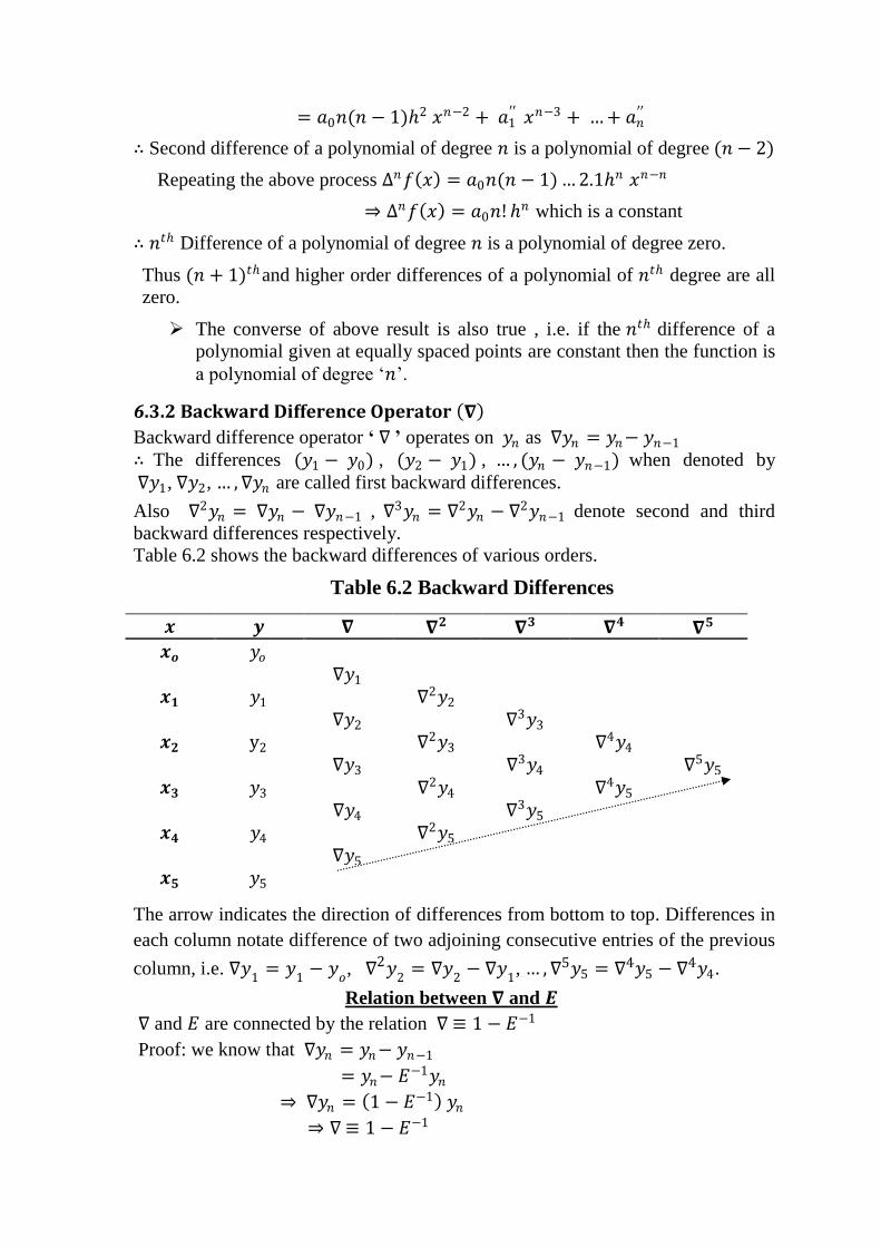
6.3.2 Backward Difference Operator 𝛁
Backward difference operator ‘ ∇ ’ operates on 𝑦𝑛 as ∇𝑦𝑛 = 𝑦𝑛− 𝑦𝑛−1
∴ The differences (𝑦1 − 𝑦0) , (𝑦2 − 𝑦1) , … , (𝑦𝑛 − 𝑦𝑛−1) when denoted by
∇𝑦1, ∇𝑦2, … ,∇𝑦𝑛 are called first backward differences.
Also ∇2𝑦𝑛 = ∇𝑦𝑛 − ∇𝑦𝑛−1 , ∇3𝑦𝑛 = ∇2𝑦𝑛 − ∇2𝑦𝑛−1 denote second and third
backward differences respectively.
Table 6.2 shows the backward differences of various orders.
Table 6.2 Backward Differences
𝒙 𝒚 𝛁 𝛁𝟐 𝛁𝟑 𝛁𝟒 𝛁𝟓 𝒙𝒐 𝑦𝑜
∇𝑦1 𝒙𝟏 𝑦1 ∇2𝑦2
∇𝑦2 ∇3𝑦3 𝒙𝟐 y2 ∇2𝑦3 ∇4𝑦4
∇𝑦3 ∇3𝑦4 ∇5𝑦5 𝒙𝟑 𝑦3 ∇2𝑦4 ∇4𝑦5
∇𝑦4 ∇3𝑦5 𝒙𝟒 𝑦4 ∇2𝑦5
∇𝑦5 𝒙𝟓 𝑦5
The arrow indicates the direction of differences from bottom to top. Differences in
each column notate difference of two adjoining consecutive entries of the previous
column, i.e. ∇𝑦1
= 𝑦1− 𝑦
𝑜, ∇2𝑦
2= ∇𝑦
2− ∇𝑦
1, … ,∇5𝑦5 = ∇4𝑦5 − ∇4𝑦4.
Relation between 𝛁 and 𝑬
∇ and 𝐸 are connected by the relation ∇ ≡ 1 − 𝐸−1
Proof: we know that ∇𝑦𝑛 = 𝑦𝑛− 𝑦𝑛−1
= 𝑦𝑛− 𝐸−1𝑦𝑛
⇒ ∇𝑦𝑛 = 1 − 𝐸−1 𝑦𝑛
⇒ ∇ ≡ 1 − 𝐸−1

6.3.3 Central Difference Operator 𝛅
Central difference operator ‘ δ ’ operates on 𝑦𝑛 as δ 𝑦𝑛 = 𝑦𝑛+
1
2
− 𝑦𝑛−
1
2
∴ The differences (𝑦1 − 𝑦0) , (𝑦2 − 𝑦1) , … , (𝑦𝑛 − 𝑦𝑛−1) when denoted by
δ𝑦1
2
, δ𝑦3
2
, … , δ𝑦𝑛−
1
2
are called first central differences.
Also δ2𝑦𝑛 = δ𝑦𝑛+
1
2
− δ𝑦𝑛−
1
2
, δ3𝑦𝑛 = δ2𝑦𝑛+
1
2
− δ2𝑦𝑛−
1
2
denote second and third
central differences respectively as shown in Table 6.3.
Table 6.3 Central Differences
𝒙 𝒚 𝛅 𝛅𝟐 𝛅𝟑 𝛅𝟒 𝛅𝟓 𝒙𝒐 𝑦𝑜
δ𝑦12
𝒙𝟏 𝑦1 δ2𝑦1
δ𝑦32 δ3𝑦3
2
𝒙𝟐 y2 δ2𝑦2 δ4𝑦
2
δ𝑦52 δ3𝑦5
2
δ5𝑦52
𝒙𝟑 𝑦3 δ2𝑦3 δ4𝑦
3
δ𝑦72 δ3𝑦7
2
𝒙𝟒 𝑦4 δ2𝑦4
δ𝑦92
𝒙𝟓 𝑦5
Central differences in each column notate difference of two adjoining consecutive
entries of the previous column, i.e. δ𝑦1
2
= 𝑦1− 𝑦
𝑜, … , δ5𝑦5
2
= δ4𝑦3 − δ4𝑦2.
Relation between 𝛅 and 𝑬
δ and 𝐸 are connected by the relation δ ≡ 𝐸1
2 − 𝐸− 1
2
Proof: we know that δ 𝑦𝑛 = 𝑦𝑛+
1
2
− 𝑦𝑛−
1
2
= 𝐸1
2𝑦𝑛− 𝐸− 1
2𝑦𝑛
⇒ δ 𝑦𝑛 = 𝐸1
2 − 𝐸− 1
2 𝑦𝑛
∴ δ ≡ 𝐸1
2 − 𝐸− 1
2
Observation: It is only the notation which changes and not the difference.
∴ 𝑦1 − 𝑦𝑜 = ∆𝑦0 = ∇𝑦1 = δ𝑦1
2
6.3.4 Averaging Operator 𝛍
Averaging operator ‘ μ ’ operates on 𝑦𝑥 as μ 𝑦𝑥 =1
2 𝑦
𝑥+
2
+ 𝑦𝑥−
2

Or μ 𝑓 𝑥 = 1
2 𝑓 𝑥 +
2 + 𝑓 𝑥 −
2 , ‘ h ’ is the height of the interval.
Relation between 𝛍 and 𝑬
We know that μ 𝑦𝑛 =1
2 𝑦
𝑛+
2
+ 𝑦𝑛−
2
=1
2 𝐸
1
2𝑦𝑛+ 𝐸− 1
2𝑦𝑛
⇒ μ 𝑦𝑛 =1
2 𝐸
1
2 + 𝐸− 1
2 𝑦𝑛
∴ μ ≡1
2 𝐸
1
2 + 𝐸− 1
2
Result 2: Relation between 𝑬 and 𝑫, where 𝑫 ≡𝒅
𝒅𝒙
We know 𝑦 𝑥 + = 𝑦 𝑥 + 𝑦′ 𝑥 +2
2! 𝑦′′ 𝑥 +. .. By Taylor’s theorem
= 𝑦 𝑥 + 𝐷𝑦(𝑥) +2
2! 𝐷2𝑦(𝑥)+. ..
= 1 + 𝐷 +2
2! 𝐷2 + ⋯ 𝑦(𝑥)
⇒ 𝐸 𝑦 𝑥 = 𝑒𝐷𝑦(𝑥)
∴ 𝐸 = 𝑒𝐷, 𝐷 ≡𝑑
𝑑𝑥
Result 3: Relation between ∆ and 𝑫, where 𝑫 ≡𝒅
𝒅𝒙
We know that ∆ ≡ 𝐸 − 1
⇒ ∆ ≡ 𝑒𝐷 − 1 ∵ 𝐸 = 𝑒𝐷
Result 4: Relation between 𝜵 and 𝑫, where 𝑫 ≡𝒅
𝒅𝒙
We know that ∇ ≡ 1 − 𝐸−1 = 1 − 𝑒−𝐷 ∵ 𝐸 = 𝑒𝐷
Result 5: Relation between ∆ and 𝜵
We know that 𝐸 ≡ 1 + ∆ ⋯①
Also 𝐸−1 ≡ 1 − ∇
⇒ 𝐸 ≡1
1−∇ ⋯ ②
⇒ 1 + ∆≡1
1−∇ From ① and ②
⇒ ∆≡1
1−∇− 1
⇒ ∆≡∇
1−∇
Result 6: Relation between 𝛍 , 𝜹 and 𝑬
We have μ ≡1
2 𝐸
1
2 + 𝐸− 1
2
Also δ ≡ 𝐸1
2 − 𝐸− 1
2
⇒ μδ ≡1
2 𝐸
1
2 + 𝐸− 1
2 𝐸1
2 − 𝐸− 1
2
⇒ μδ ≡1
2 𝐸 − 𝐸− 1
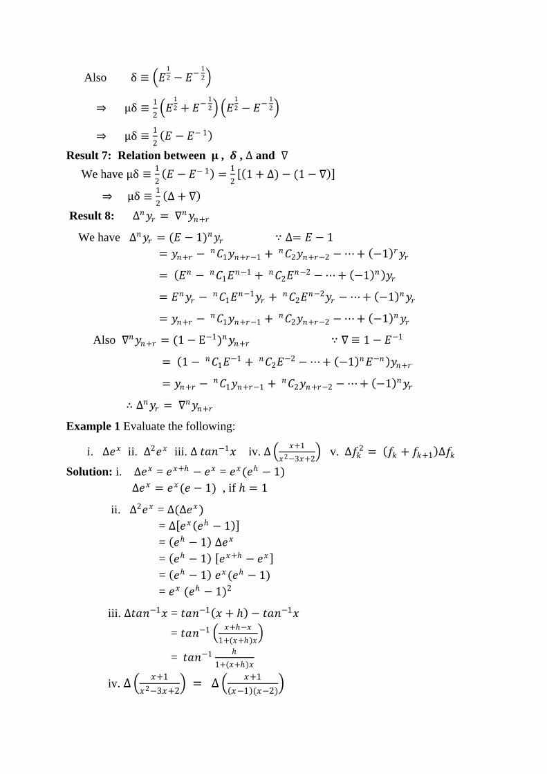
Result 7: Relation between 𝛍 , 𝜹 , ∆ and ∇
We have μδ ≡1
2 𝐸 − 𝐸− 1 =
1
2 1 + ∆) − (1 − ∇
⇒ μδ ≡1
2 ∆ + ∇
Result 8: ∆𝑛𝑦𝑟 = ∇𝑛𝑦𝑛+𝑟
We have ∆𝑛𝑦𝑟 = (𝐸 − 1)𝑛𝑦𝑟 ∵ ∆= 𝐸 − 1
= 𝑦𝑛+𝑟 − 𝑛𝐶1𝑦𝑛+𝑟−1 + 𝑛𝐶2𝑦𝑛+𝑟−2 −⋯+ −1 𝑟𝑦𝑟
= 𝐸𝑛 − 𝑛𝐶1𝐸𝑛−1 + 𝑛𝐶2𝐸
𝑛−2 −⋯+ −1 𝑛 𝑦𝑟
= 𝐸𝑛𝑦𝑟 − 𝑛𝐶1𝐸𝑛−1𝑦𝑟 + 𝑛𝐶2𝐸
𝑛−2𝑦𝑟 −⋯+ −1 𝑛𝑦𝑟
= 𝑦𝑛+𝑟 − 𝑛𝐶1𝑦𝑛+𝑟−1 + 𝑛𝐶2𝑦𝑛+𝑟−2 −⋯+ −1 𝑛𝑦𝑟
Also ∇𝑛𝑦𝑛+𝑟 = (1 − E−1)𝑛𝑦𝑛+𝑟 ∵ ∇ ≡ 1 − 𝐸−1
= 1 − 𝑛𝐶1𝐸−1 + 𝑛𝐶2𝐸
−2 −⋯+ −1 𝑛𝐸−𝑛 𝑦𝑛+𝑟
= 𝑦𝑛+𝑟 − 𝑛𝐶1𝑦𝑛+𝑟−1 + 𝑛𝐶2𝑦𝑛+𝑟−2 −⋯+ −1 𝑛𝑦𝑟
∴ ∆𝑛𝑦𝑟 = ∇𝑛𝑦𝑛+𝑟
Example 1 Evaluate the following:
i. ∆𝑒𝑥 ii. ∆2𝑒𝑥 iii. ∆ 𝑡𝑎𝑛−1𝑥 iv. ∆ 𝑥+1
𝑥2−3𝑥+2 v. ∆𝑓𝑘
2 = 𝑓𝑘 + 𝑓𝑘+1 ∆𝑓𝑘
Solution: i. ∆𝑒𝑥 = 𝑒𝑥+ − 𝑒𝑥 = 𝑒𝑥(𝑒 − 1)
∆𝑒𝑥 = 𝑒𝑥(𝑒 − 1) , if = 1
ii. ∆2𝑒𝑥 = ∆(∆𝑒𝑥)
= ∆ 𝑒𝑥 𝑒 − 1
= 𝑒 − 1 ∆𝑒𝑥
= 𝑒 − 1 𝑒𝑥+ − 𝑒𝑥
= 𝑒 − 1 𝑒𝑥(𝑒 − 1)
= 𝑒𝑥 (𝑒 − 1)2
iii. ∆𝑡𝑎𝑛−1𝑥 = 𝑡𝑎𝑛−1 𝑥 + − 𝑡𝑎𝑛−1𝑥
= 𝑡𝑎𝑛−1 𝑥+−𝑥
1+(𝑥+)𝑥
= 𝑡𝑎𝑛−1
1+(𝑥+)𝑥
iv. ∆ 𝑥+1
𝑥2−3𝑥+2 = ∆
𝑥+1
𝑥−1 (𝑥−2)

= ∆ −2
𝑥−1+
3
𝑥−2 = ∆
−2
𝑥−1 + ∆
3
𝑥−2
= −2 1
𝑥+1−1−
1
𝑥−1 + 3
1
𝑥+1−2−
1
𝑥−2
= −2 1
𝑥−
1
𝑥−1 + 3
1
𝑥−1−
1
𝑥−2
= −(𝑥+4)
𝑥 𝑥−1 (𝑥−2)
v. ∆𝑓𝑘2 = 𝑓𝑘+1
2 − 𝑓𝑘2 = 𝑓𝑘+1 + 𝑓𝑘 𝑓𝑘+1 − 𝑓𝑘 = 𝑓𝑘 + 𝑓𝑘+1 ∆𝑓𝑘
Example 2 Evaluate the following:
i. ∆𝑒𝑥 log 2𝑥 ii. ∆ 𝑥2
cos 2𝑥
Solution: i. Let 𝑓 𝑥 = 𝑒𝑥 and 𝑔 𝑥 = log 2𝑥
We have ∆ 𝑓 𝑥 𝑔 𝑥 = 𝑓 𝑥 + ∆ 𝑔 𝑥 + 𝑔 𝑥 ∆𝑓 𝑥
∴ ∆𝑒𝑥 log 2𝑥 = 𝑒𝑥+∆ log 2𝑥 + log 2𝑥 ∆𝑒𝑥
= 𝑒𝑥+ log 2 𝑥 + − log 2𝑥 + log 2𝑥 𝑒𝑥+ − 𝑒𝑥
= 𝑒𝑥𝑒 log 1 +
𝑥 + 𝑒𝑥 log 2𝑥 𝑒 − 1
= 𝑒𝑥 𝑒 log 1 +
𝑥 + log 2𝑥 𝑒 − 1
ii. Let 𝑓 𝑥 = 𝑥2 and 𝑔 𝑥 = cos 2𝑥
We have ∆ 𝑓 𝑥
𝑔 𝑥 =
𝑔 𝑥 ∆𝑓 𝑥 −𝑓(𝑥)∆𝑔 𝑥
𝑔 𝑥+ 𝑔 𝑥
=cos 2𝑥 𝑥+ 2−𝑥2 −𝑥2 cos 2 𝑥+ −cos 2𝑥
cos 2 𝑥+ cos 2𝑥
= 2+2𝑥 cos 2𝑥+2𝑥2 sin 2𝑥+ sin
cos 2 𝑥+ cos 2𝑥
Example 3 Evaluate ∆4 1 − 2𝑥 1 − 3𝑥 1 − 4𝑥 1 − 𝑥 ,where interval of differencing is one.
Solution: ∆4 1 − 2𝑥 1 − 3𝑥 1 − 4𝑥 1 − 𝑥
= ∆4 24𝑥4 + ⋯+ 1 = 24.4!. 14 = 576
∵ ∆𝑛𝑓 𝑥 = 𝑎0𝑛! 𝑛 and ∆4𝑥𝑛 = 0 when 𝑛 < 4
Example 4 Prove that ∆3𝑦3 = ∇3𝑦6
Solution: ∆3𝑦3 = (𝐸 − 1)3𝑦3 ∵ ∆= 𝐸 − 1
= 𝐸3 − 1 − 3𝐸2 + 3𝐸 𝑦3
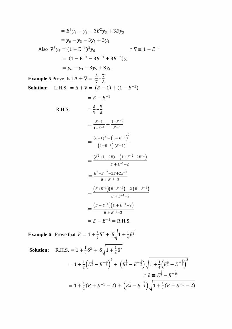
= 𝐸3𝑦3 − 𝑦3 − 3𝐸2𝑦3 + 3𝐸𝑦3
= 𝑦6 − 𝑦3 − 3𝑦5 + 3𝑦4
Also ∇3𝑦6 = (1 − E−1)3𝑦6 ∵ ∇ ≡ 1 − 𝐸−1
= 1 − E−3 − 3𝐸−1 + 3𝐸−2 𝑦6
= 𝑦6 − 𝑦3 − 3𝑦5 + 3𝑦4
Example 5 Prove that ∆ + ∇ = ∆
∇–∇
∆
Solution: L.H.S. = ∆ + ∇ = 𝐸 − 1 + 1 − 𝐸−1
= 𝐸 − 𝐸−1
R.H.S. =∆
∇–∇
∆
=𝐸−1
1−𝐸–1−
1−𝐸 –1
𝐸−1
= 𝐸−1 2 − 1− 𝐸 –1
2
1−𝐸 –1 𝐸−1
= 𝐸2+1− 2𝐸 − 1+ 𝐸–2−2𝐸–1
𝐸 + 𝐸–1−2
=𝐸2−𝐸−2−2𝐸+2𝐸–1
𝐸 + 𝐸–1−2
= 𝐸+𝐸–1 𝐸−𝐸 –1 − 2 𝐸− 𝐸–1
𝐸 + 𝐸–1−2
= 𝐸 − 𝐸–1 𝐸 + 𝐸 –1−2
𝐸 + 𝐸–1−2
= 𝐸 − 𝐸−1 = R.H.S.
Example 6 Prove that 𝐸 = 1 +1
2δ2 + δ 1 +
1
4δ2
Solution: R.H.S. = 1 +1
2δ2 + δ 1 +
1
4δ2
= 1 +1
2 𝐸
1
2 − 𝐸− 1
2 2
+ 𝐸1
2 − 𝐸− 1
2 1 +1
4 𝐸
1
2 − 𝐸− 1
2 2
∵ δ ≡ 𝐸1
2 − 𝐸− 1
2
= 1 +1
2 𝐸 + 𝐸−1 − 2 + 𝐸
1
2 − 𝐸− 1
2 1 +1
4 𝐸 + 𝐸−1 − 2
= 1 +1
2 𝐸 + 𝐸−1 − 2 + 𝐸
1
2 − 𝐸− 1
2 1
4 𝐸 + 𝐸−1 + 2
= 1 +1
2 𝐸 + 𝐸−1 − 2 + 𝐸
1
2 − 𝐸− 1
2 1
4 𝐸
1
2 + 𝐸− 1
2 2
= 1 +1
2 𝐸 + 𝐸−1 − 2 +
1
2 𝐸
1
2 − 𝐸− 1
2 𝐸1
2 + 𝐸− 1
2
=1
2 𝐸 + 𝐸−1 +
1
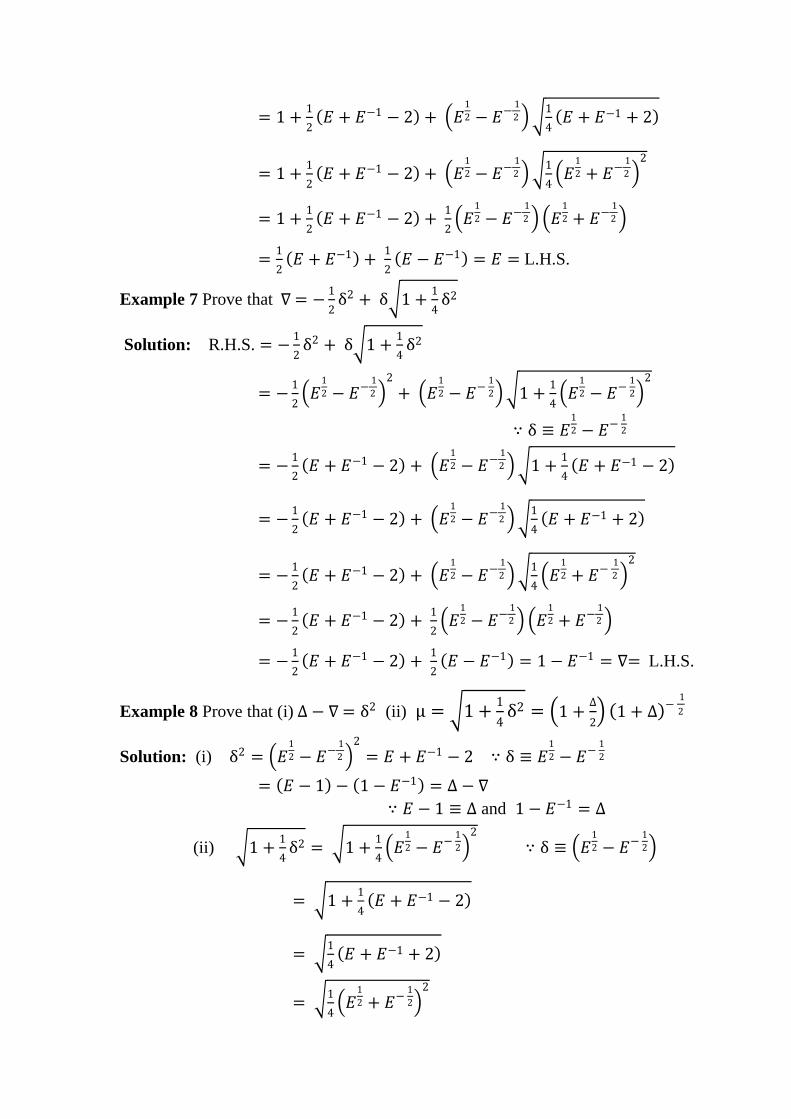
2 𝐸 − 𝐸−1 = 𝐸 = L.H.S.
Example 7 Prove that ∇ = −1
2δ2 + δ 1 +
1
4δ2
Solution: R.H.S. = −1
2δ2 + δ 1 +
1
4δ2
= −1
2 𝐸
1
2 − 𝐸− 1
2 2
+ 𝐸1
2 − 𝐸− 1
2 1 +1
4 𝐸
1
2 − 𝐸− 1
2 2
∵ δ ≡ 𝐸1
2 − 𝐸− 1
2
= −1
2 𝐸 + 𝐸−1 − 2 + 𝐸
1
2 − 𝐸− 1
2 1 +1
4 𝐸 + 𝐸−1 − 2
= −1
2 𝐸 + 𝐸−1 − 2 + 𝐸
1
2 − 𝐸− 1
2 1
4 𝐸 + 𝐸−1 + 2
= −1
2 𝐸 + 𝐸−1 − 2 + 𝐸
1
2 − 𝐸− 1
2 1
4 𝐸
1
2 + 𝐸− 1
2 2
= −1
2 𝐸 + 𝐸−1 − 2 +
1
2 𝐸
1
2 − 𝐸− 1
2 𝐸1
2 + 𝐸− 1
2
= −1
2 𝐸 + 𝐸−1 − 2 +
1
2 𝐸 − 𝐸−1 = 1 − 𝐸−1 = ∇= L.H.S.
Example 8 Prove that (i) ∆ − ∇ = δ2 (ii) μ = 1 +1
4δ2 = 1 +
∆
2 1 + ∆ −
1
2
Solution: (i) δ2 = 𝐸1
2 − 𝐸− 1
2 2
= 𝐸 + 𝐸−1 − 2 ∵ δ ≡ 𝐸1
2 − 𝐸− 1
2
= 𝐸 − 1 − 1 − 𝐸−1 = ∆ − ∇
∵ 𝐸 − 1 ≡ ∆ and 1 − 𝐸−1 = ∆
(ii) 1 +1
4δ2 = 1 +
1
4 𝐸
1
2 − 𝐸− 1
2 2
∵ δ ≡ 𝐸1
2 − 𝐸− 1
2
= 1 +1
4 𝐸 + 𝐸−1 − 2
= 1
4 𝐸 + 𝐸−1 + 2
= 1
4 𝐸
1
2 + 𝐸− 1
2 2

=1
2 𝐸
1
2 + 𝐸− 1
2 = μ ∵ μ ≡1
2 𝐸
1
2 + 𝐸− 1
2
Also 1 +∆
2 1 + ∆ −
1
2 = 1 +𝐸−1
2 1 + 𝐸 − 1 −
1
2
∵ ∆ ≡ 𝐸 − 1
= 𝐸+1
2 𝐸−
1
2
=1
2 𝐸−
1
2 + 𝐸1
2 = μ
Example 9 Prove that (i) ∆ ≡ 𝐸∇ ≡ ∇E = δ𝐸 12 (ii) Er = μ +
𝛿
2
2𝑟
Solution: (i) 𝐸∇ = E 1 − 𝐸− 1 = 𝐸 − 1 = ∆ ∵ ∇ ≡ 1 − 𝐸−1
∇E = 1 − 𝐸− 1 𝐸 = 𝐸 − 1 = ∆
δ𝐸 12 = 𝐸
1
2 − 𝐸− 1
2 𝐸 12 = 𝐸 − 1 = ∆ ∵ δ ≡ 𝐸
1
2 − 𝐸− 1
2
(ii) R.H.S. = μ +𝛿
2
2𝑟
= 1
2 𝐸
1
2 + 𝐸− 1
2 +1
2 𝐸
1
2 − 𝐸− 1
2
2𝑟
∵ μ ≡1
2 𝐸
1
2 + 𝐸− 1
2 and δ ≡ 𝐸1
2 − 𝐸− 1
2
= 1
2 2𝐸
1
2
2𝑟
= 𝐸1
2 2𝑟
= Er = L.H.S
Example 10 Prove that (i) 𝐷 ≡ 1
𝑙𝑜𝑔 𝐸 (iii) 𝐷 ≡ 𝑙𝑜𝑔 1 + ∆ ≡ −log(1 − ∇)
(iii) ∇2 ≡ 2𝐷2 − 3𝐷3 +7
124𝐷4 + ⋯
Solution: (i) We know that 𝐸 ≡ 𝑒𝐷
⇒ 𝑙𝑜𝑔𝐸 ≡ 𝑙𝑜𝑔 𝑒𝐷
⇒ 𝑙𝑜𝑔𝐸 ≡ 𝑑 𝑙𝑜𝑔 𝑒
⇒ 𝐷 ≡ 1
𝑙𝑜𝑔 𝐸 ∵ 𝑙𝑜𝑔 𝑒 = 1
(ii) 𝐷 ≡ 𝑙𝑜𝑔𝐸 From relation (i)
≡ log(1 + ∆) ∵ 𝐸 ≡ 1 + ∆
Also 𝐷 ≡ 𝑙𝑜𝑔𝐸 ≡ − log𝐸−1
≡ −log(1 − ∇) ∵ ∇ ≡ 1 − 𝐸−1
(iii) We know that ∇ ≡ 1 − 𝐸−1
⇒ ∇ ≡ 1 −1
𝐸

≡ 1 − 𝑒−𝐷 ∵ 𝐸 = 𝑒𝐷
⇒ ∇≡ 1 − 1 − 𝑑 +2𝐷2
2!−
3𝐷3
3!+ ⋯
⇒ ∇≡ 𝑑 −2𝐷2
2! +
3𝐷3
3!+ ⋯
∴ ∇2 ≡ 𝑑 −2𝐷2
2! +
3𝐷3
3!+ ⋯
2
⇒ ∇2 ≡ 2𝐷2 + 2𝐷2
2!
2
+ ⋯− 2 𝑑 2𝐷2
2! + 2 𝑑
3𝐷3
3! −⋯
⇒ ∇2 ≡ 2𝐷2 − 3𝐷3 + 4𝐷4
4+
4𝐷4
3 −⋯
⇒ ∇2 ≡ 2𝐷2 − 3𝐷3 +7
124𝐷4 −⋯
Remark: In order to prove any relation, we can express the operators (∆ ,∇,𝛿) in
terms of fundamental operator 𝐸.
Example 11 Form the forward difference table for the function
𝑓 𝑥 = 𝑥3 − 2𝑥2 − 3𝑥 − 1 for 𝑥 = 0, 1, 2, 3, 4.
Hence or otherwise find ∆3𝑓 𝑥 , also show that ∆4𝑓 𝑥 = 0
Solution: 𝑓 0 = −1, 𝑓 1 = −5, 𝑓 2 = −7, 𝑓 3 = −1, 𝑓 4 = 19
Constructing the forward difference table:
𝒙 𝒇(𝒙) ∆ ∆𝟐 ∆𝟑 ∆𝟒 𝟎 −1 −4
1 −5 2 −2 6 𝟐 −7 8 0 6 6 𝟑 −1 14 20 𝟒 19
From the table, we see that ∆3𝑓 𝑥 = 6 and ∆4𝑓 𝑥 = 0
Note: Using the formula ∆𝑛𝑓 𝑥 = 𝑎0𝑛! 𝑛 , ∆3𝑓 𝑥 = 1.3!. 1𝑛 = 6
Also ∆𝑛+1𝑓 𝑥 = 0 for a polynomial of degree 𝑛, ∴ ∆4𝑓 𝑥 = 0
Example 12 If for a polynomial, five observations are recorded as: 𝑦0 = −8,
𝑦1 = −6, 𝑦2 = 22, 𝑦3 = 148, 𝑦4 = 492, find 𝑦5.
Solution: 𝑦5 = 𝐸5𝑦0 = (1 + ∆)5𝑦0 ∵ 𝐸 ≡ 1 + ∆
= 𝑦0 + 5𝐶1∆𝑦0 + 5𝐶2∆2𝑦0 + 5𝐶3∆
3𝑦0 + 5𝐶4∆4𝑦0 + ∆5𝑦0 …①

Constructing the forward difference table:
𝒙 𝒚 ∆ ∆𝟐 ∆𝟑 ∆𝟒 𝒙𝟎 −8
2 𝒙𝟏 −6 26
28 72 𝒙𝟐 22 98 48
126 120 𝒙𝟑 148 218
344 𝒙𝟒 492
From table ∆𝑦0 = 2, ∆2𝑦0 = 26 , ∆3𝑦0 = 72 , ∆3𝑦0 = 48 … ②
⇒ 𝑦5
= −8 + 5 2 + 10 26 + 10 72 + 5 48 = 1222 using ② in ①
6.4 Missing values of Data Missing data or missing values occur when an observation is missing for a
particular variable in a data sample. Concept of finite differences can help to locate
the requisite value using known concepts of curve fitting.
To determine the equation of a line (equation of degree one), we need at least two
given points. Similarly to trace a parabola (equation of degree two), at least three
points are imperative. Thus we essentially require 𝑛 + 1 known observations to
determine a polynomial of 𝑛𝑡 degree.
To find missing values of data using finite differences, we presume the degree of
the polynomial by the number of known observations and use the result
∆𝑛+1𝑓 𝑥 = 0 for a polynomial of degree 𝑛.
Example 13 Use the concept of missing data to find 𝑦5 if 𝑦0 = −8, 𝑦1 = −6,
𝑦2 = 22, 𝑦3 = 148, 𝑦4 = 492
Solution: Constructing the forward difference table taking 𝑦5 as missing value
𝒙 𝒚 ∆ ∆𝟐 ∆𝟑 ∆𝟒 ∆𝟓 𝒙𝒐 −8
2 𝒙𝟏 −6 26
28 72 𝒙𝟐 22 98 48
126 120 𝑦5 − 1222 𝒙𝟑 148 218 𝑦5 − 1174
344 𝑦5 − 1054 𝒙𝟒 492 𝑦5 − 836
𝑦5 − 492 𝒙𝟓 𝑦5

Since 5 observations are known, let us assume that the polynomial represented by
given data is of 4𝑡 degree. ∴ ∆5𝑦 = 0 ⇒ 𝑦5− 1222 = 0 or 𝑦5 = 1222
Example 14 Find the missing values in the following table
𝒙 𝟎 𝟓 𝟏𝟎 𝟏𝟓 𝟐𝟎 𝟐𝟓
𝒇(𝒙) 6 ? 13 17 22 ?
Solution: Since there are 4 known values of 𝑓 𝑥 in the given data, let us assume
the polynomial represented by the given data to be of 3𝑟𝑑degree.
Constructing the forward difference table taking missing values as 𝑎 and 𝑏.
𝒙 𝒚 ∆ ∆𝟐 ∆𝟑 ∆𝟒 𝟎 6
𝑎 − 6 𝟓 𝑎 19 − 2𝑎
13 − 𝑎 3𝑎 − 28 𝟏𝟎 13 𝑎 − 9 38 − 4𝑎
4 10 − 𝑎 15 17 1 𝑎 + 𝑏 − 38
5 𝑏 − 28 2𝟎 22 𝑏 − 27
𝑏 − 22
25 𝑏
Since the polynomial represented by the given data is considered to be of
3𝑟𝑑degree, 4𝑡ℎand higher order differences are zero i.e. ∆4𝑦 = 0
∴ 38 − 4𝑎 = 0 and 𝑎 + 𝑏 − 38 = 0 Solving these two equations, we get 𝑎 = 9.5 𝑏 = 28.5
6.5 Finding Differences Using Factorial Notation We can conveniently find the forward differences of a polynomial using factorial
notation.
6.5.1 Factorial Notation of a Polynomial
A product of the form 𝑥 𝑥 − 1 𝑥 − 2 … 𝑥 − 𝑟 + 1 is called a factorial
polynomial and is denoted by 𝑥 𝑟
∴ 𝑥 = 𝑥
𝑥 2 = 𝑥(𝑥 − 1)
𝑥 3 = 𝑥 𝑥 − 1 (𝑥 − 2)
⋮
𝑥 𝑛 = 𝑥 𝑥 − 1 𝑥 − 2 … 𝑥 − 𝑛 + 1
In case, the interval of differencing is , then
𝑥 𝑛 = 𝑥 𝑥 − 𝑥 − … 𝑥 − 𝑛– 1

The results of differencing 𝑥 𝑟 are analogous to that differentiating 𝑥𝑟
∴ ∆ 𝑥 𝑛 = 𝑛 𝑥 𝑛−1
∆2 𝑥 𝑛 = 𝑛(𝑛 − 1) 𝑥 𝑛−2
∆3 𝑥 𝑛 = 𝑛 𝑛 − 1 (𝑛 − 2) 𝑥 𝑛−3
⋮
∆𝑛 𝑥 𝑛 = 𝑛 𝑛 − 1 𝑛 − 2 … 3.2.1 = 𝑛!
∆𝑛+1 𝑥 𝑛 = 0
Also 1
∆ 𝑥 =
𝑥 2
2 ,
1
∆ 𝑥 2 =
𝑥 3
3 and so on
1
∆2 𝑥 =
1
∆ 𝑥 2
2 =
𝑥 3
6
⋮
Remark:
i. Every polynomial of degree 𝑛 can be expressed as a factorial
polynomial of the same degree and vice-versa.
ii. The coefficient of highest power of 𝑥 and also the constant term
remains unchanged while transforming a polynomial to factorial
notation.
Example15 Express the polynomial 2𝑥2 + 3𝑥 + 1 in factorial notation.
Solution: 2𝑥2 − 3𝑥 + 1 = 2𝑥2 − 2𝑥 + 5𝑥 + 1
= 2𝑥 𝑥 − 1 + 5𝑥 + 1
= 2 𝑥 2 + 5 𝑥 + 1
Example16 Express the polynomial 2𝑥3 − 𝑥2 + 3𝑥 − 4 in factorial notation.
Solution: 2𝑥3 − 𝑥2 + 3𝑥 − 4 = 2 𝑥 3 + 𝐴 𝑥 2 + 𝐵 𝑥 − 4
Using remarks i and ii
= 2𝑥 𝑥 − 1 𝑥 − 2 + 𝐴𝑥 𝑥 − 1 + 𝐵𝑥 − 4
= 2𝑥3 + 𝐴 − 6 𝑥2 + −𝐴 + 𝐵 + 4 𝑥 − 4
Comparing the coefficients on both sides
A − 6 = −1, −𝐴 + B + 4 = 3
⇒ A = 5, B = 4
∴ 2𝑥3 − 𝑥2 + 3𝑥 − 4 = 2 𝑥 3 + 5 𝑥 2 + 4 𝑥 − 4
We can also find factorial polynomial using synthetic division as shown:
Coefficients 𝐴 and 𝐵 can be found as remainders under 𝑥2 and 𝑥 columns
𝑥3 𝑥2 𝑥
1 2 –1 3 –4
– 2 1
2 2 1 4 = 𝐵
– 4
2 5 = A

Example 17 Find ∆3𝑓 𝑥 for the polynomial 𝑓 𝑥 = 𝑥3 − 2𝑥2 − 3𝑥 − 1
Also show that ∆4𝑓 𝑥 = 0
Solution: Finding factorial polynomial of 𝑓 𝑥 as shown:
Let 𝑥3 − 2𝑥2 − 3𝑥 − 1 = 𝑥 3 + 𝐴 𝑥 2 + 𝐵 𝑥 − 1
Coefficients 𝐴 and 𝐵 can be found as remainders under 𝑥2 and 𝑥 columns
𝑥3 𝑥2 𝑥
1 1 –2 –3 –1
– 1 –1
2 1 –1 – 4 = 𝐵
– 2
1 1 = A
∴ 𝑓 𝑥 = 𝑥3 − 2𝑥2 − 3𝑥 − 1 = 𝑥 3 + 𝑥 2 − 4 𝑥 − 1
∆3𝑓 𝑥 = ∆3 𝑥 3 + 𝑥 2 − 4 𝑥 − 1
= 3! + 0 = 6 ∵ ∆𝑛 𝑥 𝑛 = 𝑛! and ∆𝑛+1 𝑥 𝑛 = 0
Also ∆4𝑓 𝑥 = ∆4 𝑥 3 + 𝑥 2 − 4 𝑥 − 1 = 0
Note: Results obtained are same as in Example 11, where we have used
forward difference table to compute the differences.
Example 18: Obtain the function whose first difference is 8𝑥3 − 3𝑥2 + 3𝑥 − 1
Solution: Let 𝑓 𝑥 be the function whose first difference is 8𝑥3 − 3𝑥2 + 3𝑥 − 1
⇒ ∆𝑓 𝑥 = 8𝑥3 − 3𝑥2 + 3𝑥 − 1
Let 8𝑥3 − 3𝑥2 + 3𝑥 − 1 = 8 𝑥 3 + 𝐴 𝑥 2 + 𝐵 𝑥 − 1
Coefficients 𝐴 and 𝐵 can be found as remainders under 𝑥2 and 𝑥 columns
𝑥3 𝑥2 𝑥
1 8 –3 3 –1
– 8 5
2 8 5 8 = 𝐵
– 16
8 21 = A
∴ ∆𝑓 𝑥 = 8𝑥3 − 3𝑥2 + 3𝑥 − 1 = 8 𝑥 3 + 21 𝑥 2 + 8 𝑥 − 1
𝑓 𝑥 = 1
∆ 8 𝑥 3 + 21 𝑥 2 + 8 𝑥 − 1
=8 𝑥 4
4+
21 𝑥 3
3+
8 𝑥 2
2− 𝑥 ∵
1
∆ 𝑥 =
𝑥 2
2 ,
1
∆ 𝑥 2 =
𝑥 3
3, …
= 2 𝑥 4 + 7 𝑥 3 + 4 𝑥 2 − [𝑥] = 2𝑥 𝑥 − 1 𝑥 − 2 𝑥 − 3 + 7𝑥 𝑥 − 1 𝑥 − 2 + 4𝑥 𝑥 − 1 − 𝑥
= 𝑥 2 𝑥 − 1 𝑥 − 2 𝑥 − 3 + 7 𝑥 − 1 𝑥 − 2 + 4 𝑥 − 1 − 1 = 𝑥 2𝑥3 − 5𝑥2 + 5𝑥 − 3 = 2𝑥4 − 5𝑥3 + 5𝑥2 − 3𝑥
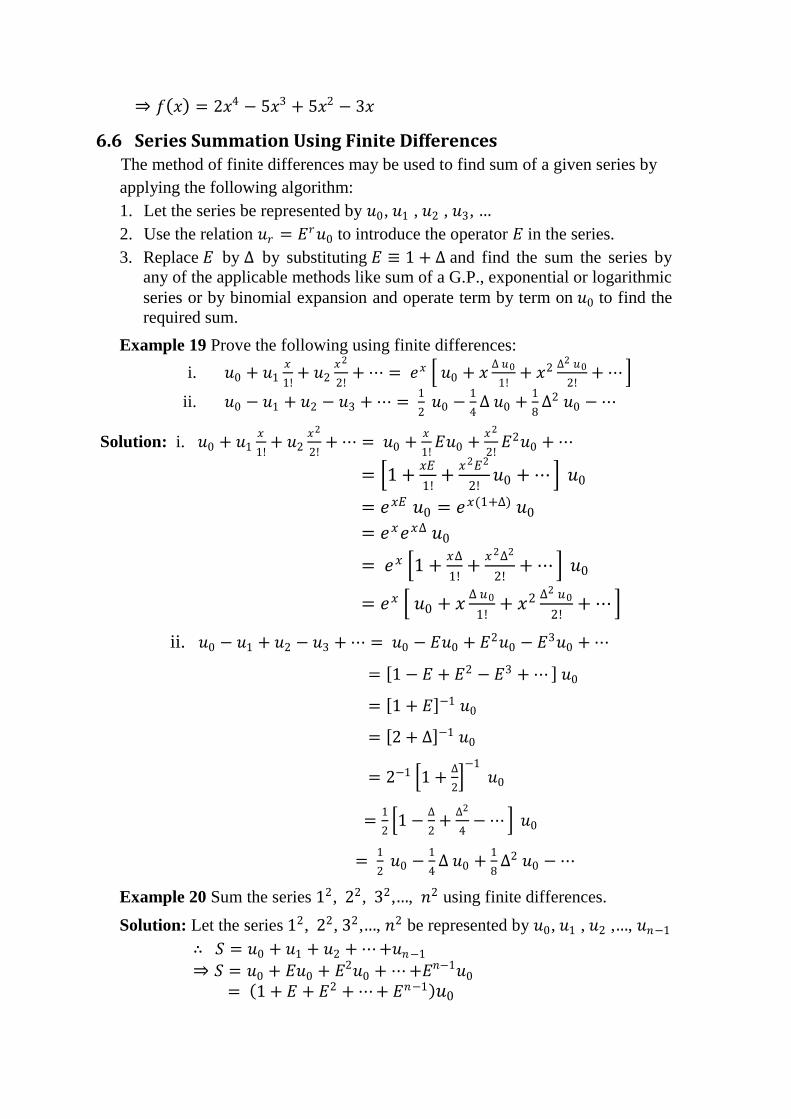
⇒ 𝑓 𝑥 = 2𝑥4 − 5𝑥3 + 5𝑥2 − 3𝑥
6.6 Series Summation Using Finite Differences The method of finite differences may be used to find sum of a given series by
applying the following algorithm:
1. Let the series be represented by 𝑢0, 𝑢1 , 𝑢2 , 𝑢3, …
2. Use the relation 𝑢𝑟 = 𝐸𝑟𝑢0 to introduce the operator 𝐸 in the series.
3. Replace 𝐸 by ∆ by substituting 𝐸 ≡ 1 + ∆ and find the sum the series by
any of the applicable methods like sum of a G.P., exponential or logarithmic
series or by binomial expansion and operate term by term on 𝑢0 to find the
required sum.
Example 19 Prove the following using finite differences:
i. 𝑢0 + 𝑢1𝑥
1!+ 𝑢2
𝑥2
2!+ ⋯ = 𝑒𝑥 𝑢0 + 𝑥
∆ 𝑢0
1!+ 𝑥2 ∆2 𝑢0
2!+ ⋯
ii. 𝑢0 − 𝑢1 + 𝑢2 − 𝑢3 + ⋯ = 1
2 𝑢0 −
1
4∆ 𝑢0 +
1
8∆2 𝑢0 −⋯
Solution: i. 𝑢0 + 𝑢1𝑥
1!+ 𝑢2
𝑥2
2!+ ⋯ = 𝑢0 +
𝑥
1!𝐸𝑢0 +
𝑥2
2!𝐸2𝑢0 + ⋯
= 1 +𝑥𝐸
1!+
𝑥2𝐸2
2!𝑢0 + ⋯ 𝑢0
= 𝑒𝑥𝐸 𝑢0 = 𝑒𝑥(1+∆) 𝑢0
= 𝑒𝑥𝑒𝑥∆ 𝑢0
= 𝑒𝑥 1 +𝑥∆
1!+
𝑥2∆2
2!+ ⋯ 𝑢0
= 𝑒𝑥 𝑢0 + 𝑥∆ 𝑢0
1!+ 𝑥2 ∆2 𝑢0
2!+ ⋯
ii. 𝑢0 − 𝑢1 + 𝑢2 − 𝑢3 + ⋯ = 𝑢0 − 𝐸𝑢0 + 𝐸2𝑢0 − 𝐸3𝑢0 + ⋯
= 1 − 𝐸 + 𝐸2 − 𝐸3 + ⋯ 𝑢0
= 1 + 𝐸 −1 𝑢0
= 2 + ∆ −1 𝑢0
= 2−1 1 +∆
2 −1
𝑢0
=1
2 1 −
∆
2+
∆2
4−⋯ 𝑢0
= 1
2 𝑢0 −
1
4∆ 𝑢0 +
1
8∆2 𝑢0 −⋯
Example 20 Sum the series 12, 22, 32,…, 𝑛2 using finite differences.
Solution: Let the series 12, 22, 32,…, 𝑛2 be represented by 𝑢0, 𝑢1 , 𝑢2 ,…, 𝑢𝑛−1
∴ 𝑆 = 𝑢0 + 𝑢1 + 𝑢2 + ⋯+𝑢𝑛−1
⇒ 𝑆 = 𝑢0 + 𝐸𝑢0 + 𝐸2𝑢0 + ⋯+𝐸𝑛−1𝑢0
= 1 + 𝐸 + 𝐸2 + ⋯+ 𝐸𝑛−1 𝑢0

=1−𝐸𝑛
1−𝐸𝑢0 =
𝐸𝑛−1
𝐸−1𝑢0 ∵ 𝑆𝑛 = 𝑎
1−𝑟𝑛
1−𝑟
⇒ 𝑆 =(1+∆)𝑛−1
(1+∆)−1𝑢0
=1
∆ 1 + 𝑛∆ +
𝑛(𝑛−1)
2!∆2 +
𝑛 𝑛−1 (𝑛−2)
3!∆3 + ⋯ − 1 𝑢0
= 𝑛𝑢0 +𝑛(𝑛−1)
2!∆𝑢0 +
𝑛 𝑛−1 (𝑛−2)
3!∆2𝑢0 + ⋯
Now 𝑢0 = 12 = 1
∆𝑢0 = 𝑢1 − 𝑢0 = 22 − 12 = 3
∆2𝑢0 = ∆𝑢1 − ∆𝑢0 = 𝑢2 − 2𝑢1 + 𝑢0 = 32 − 2( 22) + 12 = 2
∆3𝑢0, ∆4𝑢0 … are all zero as given series is an expression of degree 2
∴ 𝑆 = 𝑛 + 𝑛(𝑛−1)
2! 3 +
𝑛 𝑛−1 (𝑛−2)
3! 2 + 0
= 𝑛 +3𝑛 𝑛−1
2+
𝑛 𝑛−1 𝑛−2
3
=1
6 6𝑛 + 9𝑛 𝑛 − 1 + 2𝑛 𝑛 − 1 𝑛 − 2
=1
6𝑛 6 + 9𝑛 − 9 + 2𝑛2 − 6𝑛 + 4
=1
6𝑛 2𝑛2 + 3𝑛 + 1 =
1
6𝑛 𝑛 + 1 (2𝑛 + 1)
Example 21 Prove that 𝑢0 + 𝑢1𝑥 + 𝑢2𝑥2 + ⋯ =
𝑢0
1−𝑥+
𝑥∆𝑢0
(1−𝑥)2+
𝑥2∆𝑢02
(1−𝑥)3+ ⋯
and hence evaluate 1.2 + 2.3𝑥 + 3.4𝑥2 + 4.5𝑥3 + ⋯
Solution: 𝑢0 + 𝑢1𝑥 + 𝑢2𝑥2 + ⋯ = 𝑢0 + 𝑥𝐸𝑢0 + 𝑥2𝐸
2𝑢0 + ⋯
= 1 + 𝑥𝐸 + 𝑥2𝐸2 + ⋯ 𝑢0
=1
1−𝑥𝐸𝑢0 ∵ 𝑆∞ =
𝑎
1−𝑟
=1
1−𝑥(1+∆)𝑢0 =
1
(1−𝑥)−𝑥∆𝑢0
=1
1−𝑥
1
1−𝑥∆
1−𝑥 𝑢0
=1
1−𝑥 1 −
𝑥∆
1−𝑥 −1𝑢0
=1
1−𝑥 1 +
𝑥∆
1−𝑥 +
𝑥2∆2
(1−𝑥)2+ ⋯ 𝑢0
= 𝑢0
1−𝑥+
𝑥∆𝑢0
(1−𝑥)2+
𝑥2∆𝑢02
(1−𝑥)3+ ⋯ = R.H.S.

Now to evaluate the series 1.2 + 2.3𝑥 + 3.4𝑥2 + 4.5𝑥3 + ⋯
Let 𝑢0 = 1.2 = 2, 𝑢1 = 2.3 = 6, 𝑢2 = 3.4 = 12, 𝑢3 = 4.5 = 20,…
Forming forward difference table to calculate the differences
𝒖 ∆ ∆𝟐 ∆𝟑 ∆𝟒 𝒖𝟎 = 𝟏.𝟐 = 𝟐
4 𝒖𝟏 = 𝟐.𝟑 = 𝟔 2
6 0 𝒖𝟐 = 𝟑.𝟒 = 𝟏𝟐 2 0
8 0 𝒖𝟑 = 𝟒.𝟓 = 𝟐𝟎 2
10 𝒖𝟒 = 𝟓.𝟔 = 𝟑𝟎
∴ 1.2 + 2.3𝑥 + 3.4𝑥2 + 4.5𝑥3 + ⋯ = 𝑢0
1−𝑥+
𝑥∆𝑢0
(1−𝑥)2+
𝑥2∆𝑢02
(1−𝑥)3+ ⋯
=2
1−𝑥+
4𝑥
(1−𝑥)2+
2𝑥2
(1−𝑥)3+ 0
=2
(1−𝑥)3
Exercise 6A
1. Express 𝑦4 in terms of successive forward differences.
2. Prove that ∆𝑛𝑒3𝑥+5 = 𝑒3 − 1 𝑛𝑒3𝑥+5
3. Evaluate ∆2 5𝑥+12
𝑥2+5𝑥+6
4. If 𝑢0 = 3, 𝑢1 = 12, 𝑢2 = 81, 𝑢3 = 2000, 𝑢4 = 100, calculate ∆4𝑢0.
5. Prove that μ =2+∆
2 1+∆= 1 +
1
4δ2
6. Find the missing value in the following table
𝑥 0 5 10 15 20 25
𝑦 6 10 - 17 - 31
7. Sum the series 13, 23, 33,…, 𝑛3 using finite differences.
Answers
1. 𝑦4 = 𝑦0 + 4∆𝑦0 + 6∆2𝑦0 + 4∆3𝑦0 + ∆4𝑦0
3. –3(𝑥2+9𝑥+15)
𝑥(𝑥+1)(𝑥+4)(𝑥+5)(𝑥+8)(𝑥+9)
4. −7459
6. 13.25, 22.5


