

FEDERAL UNIVERSITY OF TECHNOLOGY - PARANÁ
GRADUATE PROGRAM IN ELECTRICAL AND COMPUTER ENGINEERING
GUILHERME HEIM WEBER
CHARACTERIZATION OF TRANSMISSION LINES BASED ON
FREQUENCY-DOMAIN AND TIME-DOMAIN MEASUREMENT
TECHNIQUES
MASTER THESIS
CURITIBA
2018

GUILHERME HEIM WEBER
CHARACTERIZATION OF TRANSMISSION LINES BASED ON
FREQUENCY-DOMAIN AND TIME-DOMAIN MEASUREMENT
TECHNIQUES
Master thesis submitted to the Graduate
Program in Electrical and Computer
Engineering of Federal University –
Paraná, as a partial requirement for the
degree of Master of Science – Concentration
Area: Automation and Systems
Engineering.
Advisor: Prof. Marco José da Silva, Dr.
Co-advisor: Prof. Cicero Martelli, Dr.
CURITIBA
2018

Dados Internacionais de Catalogação na Publicação
Weber, Guilherme Heim W374c Characterization of transmission lines based on frequency- 2018 -domain and time-domain measurement techniques / Guilherme
Heim Weber.-- 2018. 86 f. : il. ; 30 cm Disponível também via World Wide Web Texto em inglês com resumo em português Dissertação (Mestrado) - Universidade Tecnológica Federal
do Paraná. Programa de Pós-graduação em Engenharia Elétrica e Informática Industrial, Curitiba, 2018
Bibliografia: f. 81-86 1. Linhas elétricas. 2. Linhas de telecomunicação. 3. Cabos
elétricos. 4. Condutores elétricos. 5. Cabos de telecomunicação. 6. Engenharia elétrica - Dissertações. I. Silva, Marco José da. II. Martelli, Cicero. III. Universidade Tecnológica Federal do Paraná. Programa de Pós-Graduação em Engenharia Elétrica e Informática Industrial. IV. Título.
CDD: Ed. 23 – 621.3
Biblioteca Central da UTFPR, Câmpus Curitiba Bibliotecário: Adriano Lopes CRB-9/1429

Ministério da Educação Universidade Tecnológica Federal do Paraná Diretoria de Pesquisa e Pós-Graduação
TERMO DE APROVAÇÃO DE DISSERTAÇÃO Nº 797
A Dissertação de Mestrado intitulada “Characterization of Transmission Lines Based on Frequency-domain and Time-domain measurement techniques” defendida em sessão pública pelo(a) candidato(a) Guilherme Heim Weber, no dia 21 de maio de 2018, foi julgada para a obtenção do título de Mestre em Ciências, área de concentração Engenharia de Automação e Sistemas, e aprovada em sua forma final, pelo Programa de Pós-Graduação em Engenharia Elétrica e Informática Industrial.
BANCA EXAMINADORA:
Prof(a). Dr(a). Marco José da Silva - Presidente – (UTFPR) Prof(a). Dr(a). Eduardo Nunes dos Santos - (UTFPR)
Prof(a). Dr(a). Daniel Discini Silveira - (UFJF)
A via original deste documento encontra-se arquivada na Secretaria do Programa, contendo a
assinatura da Coordenação após a entrega da versão corrigida do trabalho.
Curitiba, 21 de maio de 2018.

ACKNOWLEDGMENTS
I would like to acknowledge Petrobras ad National Agency of Petroleum, Natural
Gas and Biofuels for providing financial resources for this study.
My deepest gratitude to my advisor Professor Dr. Marco José da Silva for all the
effort, patience and time dedicated to me and to this work, for being my mentor
through the academic research. My gratitude to co-advisor Professor Dr. Cicero
Martelli and Professor Dr. Jean Cardozo, who actively participated in the development
of this work. Special thanks to Professor Dr. Daniel Pipa for providing knowledge to
develop the solution of the proposed method in this work.
My gratitude to my family for all the support and encouragement during the
masters, especially to my parents Matias Weber and Cleís Heim who always have kept
me up and have shown me the right way. Thanks to my sisters Fernanda, Katherine
and Flávia for always supporting me and caring about me.
My gratitude to Gabriella Kesikowski for always being by my side and motivating
me during the development of this work.
My gratitude to my friends Jean Nakatu, Eduardo Nunes, Aluísio Wrasse, Tiago
Venduscolo, Guilherme Dutra, Uilian Dreyer, Rafael Daciuk, Hector Lise, Eduardo
Robin and André Di Renzo, for always being by my side and providing support.

ABSTRACT
WEBER, G. H.. Characterization of transmission lines based on frequency-domain
and time-domain measurement techniques. 86 p. Master Thesis - Graduate Program
in Electrical and Computer Engineering of Federal University of Technology –
Paraná. Curitiba, 2018.
The importance of electrical cables in modern data communication and power
transmission systems cannot be overstated. Efficient and secure transmission of either
data or energy depends on the healthy state of electrical cables and cable networks. In
many applications, the continuous monitoring of cable characteristics is required in
order to guarantee system performance. In this work, different time-domain and
frequency domain techniques are applied to a set of experiments to explore different
means to characterize transmission lines in a comparative manner. First, two exemplary
cables are analyzed by frequency domain techniques to obtain their capacities in
function of different cable lengths. Results show the influence of length over channel
capacity for both cables, which were compared to commercial data transmission
systems. As a second part of the experiments, a chosen cascaded transmission line set
is characterized in time and frequency domain. Time domain analysis based on
reflectometry and transmissometry methods reveals impedance mismatches along the
line and impulse response respectively. Frequency domain analysis is based on the
scattering parameters and enables the extraction of the electrical parameters of the
channel. Also, time domain analysis of scattering parameters can be performed by the
inverse chirp Z transform, a weak approach generally based on a minimum norm
solution. Since the nature of the impedance mismatches along the line is sparse, it is
proposed a sparse inverse chirp Z transform, specially designed for this kind of
application. The method is verified by comparing results provided by the general
approach, showing promising performance through the reflection and transmission
profiles obtained.
Keywords: inverse chirp Z transform, frequency domain analysis, scattering
parameters, time domain analysis, transmission line analysis.

RESUMO
WEBER, G. H.. Caracterização de linhas de transmissão baseada em técnicas de
medição no domínio do tempo e no domínio da frequência. 86 f. Dissertação de
Mestrado - Programa de Pós-Graduação em Engenharia Elétrica e Engenharia de
Computação da Universidade Tecnológica Federal do Paraná. Curitiba, 2018.
A importância de cabos elétricos em sistemas modernos de comunicação de dados
e transmissão de energia não pode ser subestimada. A transmissão segura e eficiente de
dados ou energia depende da integridade dos cabos elétricos e redes de cabos. Em
muitas aplicações o monitoramento contínuo das características do cabo é necessário
para garantir o desempenho do sistema. Neste trabalho, diferentes técnicas no domínio
do tempo e no domínio da frequência são aplicadas a um conjunto de experimentos
para explorar diferentes meios para caracterizar linhas de transmissão de forma
comparativa. Primeiro, dois cabos exemplares são analisados por técnicas no domínio
da frequência para obter suas capacidades em função de diferentes comprimentos de
cabo. Os resultados mostram a influência do comprimento sobre a capacidade do canal
para ambos os cabos, os quais foram comparados a sistemas comerciais de transmissão
de dados. Como segunda parte dos experimentos, um conjunto de linhas de transmissão
em cascata escolhido é caracterizado no domínio do tempo e da frequência. A análise
do domínio do tempo baseada em métodos de reflectometria e transmissometria revela
descasamentos de impedância ao longo da linha e resposta ao impulso, respectivamente.
A análise no domínio da frequência é baseada nos parâmetros de espalhamento e
permite a extração dos parâmetros elétricos do canal. Além disso, a análise no domínio
do tempo dos parâmetros de espalhamento pode ser realizada pela transformada inversa
chirp Z, uma abordagem fraca geralmente baseada em uma solução de norma mínima.
Uma vez que a natureza dos descasamentos de impedância ao longo da linha é esparsa,
propõe-se uma transformada inversa chirp Z esparsa, especialmente projetada para este
tipo de aplicação. O método é verificado comparando-se os resultados fornecidos pela
abordagem geral, mostrando desempenho promissor através dos perfis de reflexão e
transmissão obtidos.

Palavras-chave: transformada inversa chirp Z, análise no domínio da
frequência, parâmetros S, análise no domínio do tempo, análise de linhas de
transmissão.

LIST OF FIGURES
Figure 1 – Transmission line lumped model: (a) voltage and current definitions; (b)
lumped-element equivalent circuit (POZAR, 2005). .................................................. 26
Figure 2 - Transmission line terminated in a load impedance ZL (POZAR, 2005). .... 29
Figure 3 - Locations of maximum and minimum standing wave values along the line
toward the generator (IDA, 2015). ............................................................................ 32
Figure 4 - Two-port network model for system connected to a source and load.
Adapted from (BEGOVIC; SKALJO; GORAN, 2013). ............................................. 33
Figure 5 - Different shapes of reflections and their meanings (AGILENT
TECHNOLOGIES, 2012). ......................................................................................... 37
Figure 6 - Scattering parameters measurement topology for 2-port network. ............ 39
Figure 7 - Chirp Z Transform: spiral contour in the Z plane. Adapted from
(RABINER; SCHAFER; RADER, 1969). ................................................................. 41
Figure 8 – Two-port network - ABCD matrix representation. .................................. 42
Figure 9 - Two-port networks in cascaded connection. .............................................. 43
Figure 10 – Frequency selective fading channel (GOLDSMITH, 2005). .................... 45
Figure 11 - Block diagram of basic OFDM system. Adapted from (BAHAI;
SALTZBERG; ERGEN, 2004). ................................................................................. 47
Figure 12 –Cables selected for analysis: CAT5e UTP line (a) and flexible stranded
two-wire copper 1.5 mm² (b). .................................................................................... 51
Figure 13 - Channel set chosen to be characterized in time and frequency domain. .. 52
Figure 14 - Block diagram for the channel analysis proposed. ................................... 53
Figure 15 – Time domain measurements scenario: reflectometry profile acquisition (a)
and transmissometry profile acquisition (b). .............................................................. 57
Figure 16 - Frequency response of the twisted-pair line for the different length sets, in
dB. ............................................................................................................................. 59
Figure 17 - Channel capacity and performance of the twisted-pair channel. ............. 60
Figure 18 - Frequency response of the two-wire line, in dB. ...................................... 61
Figure 19 - Channel capacity and performance of the two-wire channel. .................. 62

Figure 20 - TDR profiles of the channel under test in direct perspective using
different pulse widths and different terminations. (a) presents the profiles obtained
with the pulse 1.5 ns wide for open, short and load termination, (b) the profile
obtained with the pulse 5 ns wide for each termination, and (c) the profiles using the
pulse 10 ns wide. The y axis represents the magnitude of the reflection coefficients
along the channel over time. ...................................................................................... 64
Figure 21 - TDR profiles of the channel under test in reverse perspective using
different pulse widths and different terminations. (a) shows the profiles obtained with
the pulse 1.5 ns wide for open, short and load termination, (b) the profile obtained
with the pulse 5 ns wide for each termination, and (c) the profiles using the pulse 10
ns wide. The y axis represents the magnitude of the reflection coefficients along the
channel, given in time (x axis). ................................................................................. 66
Figure 22 - Impulse response of the channel under analysis. (a) depicts the response
considering the propagation through the direct perspective, while (b) for the contrary
perspective. ................................................................................................................ 68
Figure 23 - S21 parameter acquired for the analysis of the channel under test. (a)
depicts the magnitude of the parameter, in dB. (b) presents its angle over the
frequency, in rad. ....................................................................................................... 69
Figure 24 – S11 parameter acquired for the analysis of the channel under test. (a)
depicts the magnitude of the parameter, in dB. (b) presents its angle over the
frequency, in rad. ....................................................................................................... 70
Figure 25 – Analysis of the parameters S11 and S22 in time domain, given by the
conversion performed by ICZT and Sparse ICZT, in comparison to the TDR profile
acquired. (a) is related to the direct perspective of the channel, whereas (b) to the
reverse perspective. .................................................................................................... 71
Figure 26 - Analysis of the parameters S21 and S12 in time domain, presenting results
of the conversion performed by ICZT and Sparse ICZT, in comparison to the TDT
profile acquired. (a) presents the parameter S21 in time domain, related to the direct
perspective propagation. (b) presents the parameter S12 in time domain, related to
the reverse perspective propagation. .......................................................................... 74
Figure 27 - Characteristic impedance of the cascaded transmission line under analysis
calculated from the scattering parameters acquired. .................................................. 75

Figure 28 - Propagation constant calculated from the scattering parameters acquired
of the mixed channel. The attenuation constant alpha (a) (real part of the
propagation constant) increases with the frequency, standing near to 0.017 at 100
MHz. The phase constant beta (b) (imaginary part) varies periodically following the
length of the channel under test. ............................................................................... 76
Figure 29 - Distributed parameters calculated for the channel under analysis. (a)
depicts the distributed resistance given in .m-1, (b) the distributed inductance in µ
H.m-1, (c) the distributed conductance in m S.m-1, and (d) the distributed capacitance
in p F.m-1. .................................................................................................................. 77
Figure 30 - Frequency response of the channel under analysis, in dB. ....................... 78
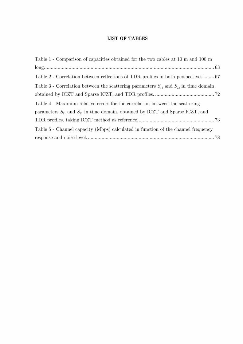
LIST OF TABLES
Table 1 - Comparison of capacities obtained for the two cables at 10 m and 100 m
long. ........................................................................................................................... 63
Table 2 - Correlation between reflections of TDR profiles in both perspectives. ....... 67
Table 3 - Correlation between the scattering parameters S11 and S22 in time domain,
obtained by ICZT and Sparse ICZT, and TDR profiles. ........................................... 72
Table 4 - Maximum relative errors for the correlation between the scattering
parameters S11 and S22 in time domain, obtained by ICZT and Sparse ICZT, and
TDR profiles, taking ICZT method as reference. ....................................................... 73
Table 5 - Channel capacity (Mbps) calculated in function of the channel frequency
response and noise level. ............................................................................................ 78

NOMENCLATURE
ADSL Assymetric Digital Subscriber Line
AV Audio Video
AWGN Additive White Gaussian Noise
BPSK Binary Phase Shift Keying
CAT5e ANSI/TIA/EIA-568-A 5e Cable Category
CSMA/CA Carrier Sense Multiple Acces / Collision Avoidance
CZT Chirp Z Transform
DAB Digital Audio Broadcasting
DFT Discrete Fourier Transform
DMT Discrete Multitone
DSL Digital Subscriber Line
DVB Digital Video Broadcasting
FDR Frequency Domain Reflectometry
FFT Fast Fourier Transform
FISTA Fast Iterative Shrinkage-Thresholding Algorithm
HF High Frequency (3 MHz to 30 MHz)
ICZT Inverse Chirp Z Transform
IFFT Inverse Fast Fourier Transform
IS Impedance Spectroscopy
ISI Intersymbol Interference
ITU International Telecommunications Union
MAC Media Access Control
MF Medium Frequency (300 kHz to 3 MHz)
MIMO Multiple Input Multiple Output
MPDU MAC Protocol Data Unit
OFDM Orthogonal Frequency Domain Multiplexing
PBs PHY Blocks
PHY Physical layer
PLC Power Line Communication
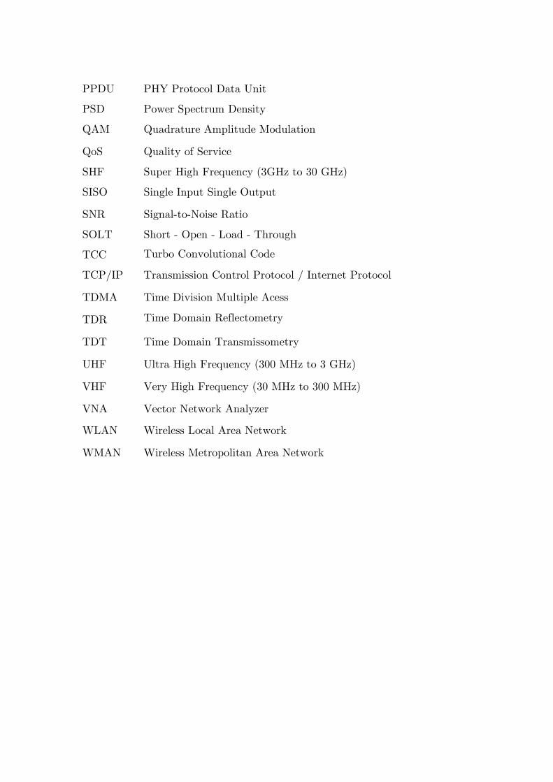
PPDU PHY Protocol Data Unit
PSD Power Spectrum Density
QAM Quadrature Amplitude Modulation
QoS Quality of Service
SHF Super High Frequency (3GHz to 30 GHz)
SISO Single Input Single Output
SNR Signal-to-Noise Ratio
SOLT Short - Open - Load - Through
TCC Turbo Convolutional Code
TCP/IP Transmission Control Protocol / Internet Protocol
TDMA Time Division Multiple Acess
TDR Time Domain Reflectometry
TDT Time Domain Transmissometry
UHF Ultra High Frequency (300 MHz to 3 GHz)
VHF Very High Frequency (30 MHz to 300 MHz)
VNA Vector Network Analyzer
WLAN Wireless Local Area Network
WMAN Wireless Metropolitan Area Network
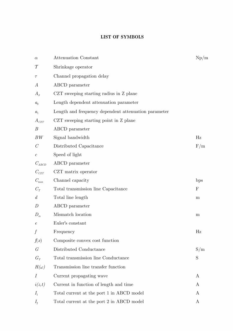
LIST OF SYMBOLS
Attenuation Constant Np/m
Shrinkage operator
Channel propagation delay
A ABCD parameter
A0 CZT sweeping starting radius in Z plane
a0 Length dependent attenuation parameter
a1 Length and frequency dependent attenuation parameter
ACZT CZT sweeping starting point in Z plane
B ABCD parameter
BW Signal bandwidth Hz
C Distributed Capacitance F/m
c Speed of light
CABCD ABCD parameter
CCZT CZT matrix operator
Cmax Channel capacity bps
CT Total transmission line Capacitance F
d Total line length m
D ABCD parameter
Dm Mismatch location m
e Euler's constant
f Frequency Hz
f(x) Composite convex cost function
G Distributed Conductance S/m
GT Total transmission line Conductance S
H() Transmission line transfer function
I Current propagating wave A
i(z,t) Current in function of length and time A
I1 Total current at the port 1 in ABCD model A
I2 Total current at the port 2 in ABCD model A

I3 Total current at the port 3 in ABCD model A
IL Current at the load A
j Imaginary Unit
k Step number for the proximal regularization solution
kf Exponent of the attenuation factor
ks Convergence order parameter related to the number of steps
L Distributed Inductance H/m
l Length refeered to the load m
LB Blind spot length m
lmax Location of maximum value of voltage wave (in units of wave
length)
lmin Location of minimum value of voltage wave (in units of wave
length)
LT Total transmission line Inductance H
N Additive white Gaussian noise power level W
O Convergence order parameter
R Distributed Resistance /m
RL Return loss dB
RT Total transmission line Resistance
S Average signal power W
S Scattering parameters matrix
S11 Input reflection coefficient with matched output
S12 Reverse transmission coefficient with matched input
S21 Forward transmission coefficient with matched output
S22 Output reflection coefficient with matched input
SWR Standing Wave Ratio
t Time s
tk Step size for proximal regularization solution
tResolution TDR time resolution s
twidth Interrogation pulse width s
V Voltage propagating wave V
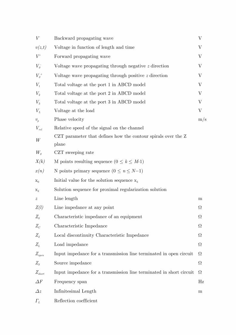
V- Backward propagating wave V
v(z,t) Voltage in function of length and time V
V+ Forward propagating wave V
V0- Voltage wave propagating through negative z direction V
V0+ Voltage wave propagating through positive z direction V
V1 Total voltage at the port 1 in ABCD model V
V2 Total voltage at the port 2 in ABCD model V
V3 Total voltage at the port 3 in ABCD model V
VL Voltage at the load V
vp Phase velocity m/s
Vrel Relative speed of the signal on the channel
W CZT parameter that defines how the contour spirals over the Z
plane
W0 CZT sweeping rate
X(k) M points resulting sequence (0 k M-1)
x(n) N points primary sequence (0 n N1
x0 Initial value for the solution sequence xk
xk Solution sequence for proximal regularization solution
z Line length m
Z(l) Line impedance at any point
Z0 Characteristic impedance of an equipment
ZC Characteristic Impedance
Zd Local discontinuity Characteristic Impedance
ZL Load impedance
Zopen Input impedance for a transmission line terminated in open circuit
ZS Source impedance
Zshort Input impedance for a transmission line terminated in short circuit
DF Frequency span Hz
Dz Infinitesimal Length m
GL Reflection coefficient

G(l) Reflection coefficient at any point
Phase Constant rad/m
Propagation Constant
0 CZT sweeping angle step size rad
Wave length m
CZT Regularization parameter of L2-L1 minimization problem solution
Set of real numbers
0 CZT sweeping starting angle in Z plane rad
G Reflection coefficient phase angle rad
G(l) Reflection coefficient at any point phase angle rad
Reflection coefficient
Angular Frequency rad/s
CONTENTS
1 INTRODUCTION ................................................................................................21
1.1 MOTIVATION .................................................................................................21
1.2 OBJECTIVES ...................................................................................................23
1.2.1 General Objective ............................................................................................23
1.2.2 Specific Objectives ..........................................................................................23
1.3 STRUCTURE ...................................................................................................24
2 THEORETICAL BACKGROUND .......................................................................25
2.1 TRANSMISSION LINES ..................................................................................25
2.1.1 The Lumped Model .........................................................................................25
2.1.2 The Load Reflection Coefficient ......................................................................29
2.1.3 Line Impedance and the Generalized Reflection Coefficient ............................29
2.1.4 The Terminated Lossless Transmission Line ...................................................30
2.1.5 Transmission Line Transfer Function .............................................................33
2.2 NETWORK ANALYSIS ...................................................................................33
2.2.1 Time Domain Reflectometry ...........................................................................34
2.2.2 Scattering Parameters .....................................................................................38
2.2.2.1 Scattering parameters in time domain .........................................................40
2.2.3 ABCD Matrix .................................................................................................42
2.2.4 Impedance Spectroscopy .................................................................................44
2.2.5 Shannon-Hartley Theorem ..............................................................................44
2.2.6 LTI Channel Model .........................................................................................45
2.3 ORTHOGONAL FREQUENCY DIVISION MULTIPLEXING .......................46
2.3.1 Power Line Communication ............................................................................47
2.3.1.1 HomePlug AV2 ...........................................................................................48
3 METHODOLOGY ................................................................................................50
3.1 INFLUENCE OF THE LENGTH OVER THE CHANNEL CAPACITY SET 50
3.2 CHANNEL ANALYSIS THROUGH TIME DOMAIN AND FREQUENCY
DOMAIN DATA .....................................................................................................52

3.2.1 Frequency Domain Data Acquisition and Analysis .........................................53
3.2.1.1 Sparse Inverse Chirp-Z Transform for Time Domain Analysis ....................54
3.2.2 Time Domain Data Acquisition and Analysis .................................................56
4 RESULTS AND DISCUSSIONS ..........................................................................59
4.1 CHANNEL CAPACITY IN DIFFERENT LENGTHS .....................................59
4.1.1 Twisted-Pair Line ...........................................................................................59
4.1.2 Two-Wire Stranded Line .................................................................................61
4.2 CHANNEL ANALYSIS IN TIME AND FREQUENCY DOMAIN ..................64
4.2.1 Time Domain Results ......................................................................................64
4.2.2 Frequency Domain Results..............................................................................69
5 CONCLUSIONS ...................................................................................................79
5.1 FUTURE WORK..............................................................................................80
REFERENCES ........................................................................................................81

21
1 INTRODUCTION
1.1 MOTIVATION
The use of electrical cables to transmit data or energy has steadily grown in the
past due to the fast expansion of the demand on energy and communication industries.
Current end-consumer or industrial systems demand transmission rates greater than
ever existed as well as more efficient power transmission through smaller, less
susceptible to electromagnetic interference and less noise generating transmission lines.
Several applications come up with different issues such as cable attenuation,
possible impedance mismatches along the channel, faults, electromagnetic susceptibility
and thermal noise. Cables faults (sometimes intermittent) can cause power failure or
loss of control, giving the importance of monitoring the integrity of the cables
(YAMADA; HIRAI; OHKI, 2012). On the aircrafts industry, typically there are several
tens of miles of wires within their structures (BLEMEL; FURSE, 2001), and wiring
problems have already been identified as the likely cause of several accidents (SMITH;
FURSE; GUNTHER, 2005). Among the wiring problems there are wire insulation
chafing, defective connections, ticking short circuits, solid short circuits, insulation
breakdown, exposed conductors and corrosion (BLEMEL; FURSE, 2001). Once placed
on their designated positions such problems often cannot be identified and fixed. The
mechanical structure on these kind of environments does not allow visual inspection or
any direct located measuring.
In the oil industry, for example, there is a need for measuring and registering oil
reservoir’s characteristics of offshore wells. Subsea installations imply in some
restrictions on the electrical cables for communications systems and electrical power
energy distribution which supply down-hole electronics and tools (RITO et al., 2013).
Hence, the development of systems like those demands a prior knowledge about the
electrical parameters of existing cable structures and in some application the need for
continuous monitoring of electrical cables and their current transmission performance.
In a communication system for example, is essential to know the maximum possible
capacity to achieve through a given channel. Current communication technologies like
Orthogonal Frequency Domain Multiplexing (OFDM) and Turbo Convolutional Code
(TCC) provides robust performance within 0.5 dB of Shannon’s limit (ALLIANCE;

22
RESERVED, 2005), implying on the importance of knowing the channel capacity of a
target transmission line and on the efficiency of the application at all.
This scenario opens horizons for methods for detecting faults on cable and/or its
current transmission capacity. The most known and applied so far are reflectometry
based methods like time-domain reflectometry (TDR), frequency-domain reflectometry
(FDR) (CHING-WEN HSUE; TE-WEN PAN, 1997) (VANHAMME, 1990), time
gating methods (DUNSMORE; CHENG; ZHANG, 2011), and identification of
moderate reflections of cascaded circuits by transmission and reflection measurements
(VEIJOLA; VALTONEN, 1988). The main idea of all those techniques consists in
applying a high frequency stimulus to the line and monitor the reflected signals
generated by impedance mismatches. Although their success on this field, most of
reflectometry based methods have a restricted application given by certain assumptions
such as small amplitudes for the reflections (VEIJOLA; VALTONEN, 1988) (VAN
HAMME, 1992) or prior knowledge about the line under test (VANHAMME, 1990).
Recently a method based on a sample maximum likelihood estimator for locating and
separating closely spaced reflections with high magnitude has been proposed (ZYARI;
ROLAIN, 2016), at the expense of an increase in complexity of the model yet. Another
technique for characterizing transmission lines is called impedance spectroscopy (IS),
which consists in measuring the impedance of the line under test in a given frequency
spectrum with one end terminated in short and open circuit. From these measurements
it is calculated the parameters characteristic impedance and propagation constant, and
from these the primary ones, composing a model of the line over the frequency spectrum
acquired (SHI; KANOUN, 2013). Impedance spectroscopy also enables the analysis of
the line in time domain, allowing to identify faults along it .(QINGHAI SHI; KANOUN,
2015).
Despite of its simple concept, time-domain methods come up with limitations on
signal detection, implying a restriction on the application to monitor weak impedance
mismatches or at high noisy and high attenuation systems (AGILENT
TECHNOLOGIES, 2012). Moreover, they require ideal open and short terminations,
which are difficult to achieve over a broadband frequency range. Due to electric field
fringing at high frequencies, open circuit terminations cause stray capacitance, and
short circuit terminations introduce additional inductance to the line (PAPAZYAN et
al., 2004). These problems on measurements are also related to the IS method.
Facing all these facts, the concept of travelling waves for the analysis of
transmission lines becomes an attractive alternative. The scattering parameters, basis
23
of this analysis, do not depend on terminations but only on incident, scattered and
reflected waves over the network. The parameters are acquired on frequency domain
at one frequency at a time using a vector network analyzer, which provides high signal-
to-noise ratio and high frequency resolution over a wide bandwidth. In addition, the
analysis of the network in time domain though the scattering parameters is possible,
and is given by the conversion through the Inverse Chirp Z Transform (RABINER;
SCHAFER; RADER, 1969), first proposed in 1969 and already used by commercial
instruments.
1.2 OBJECTIVES
1.2.1 General Objective
Facing the importance of studying and monitoring electrical cables and cables
networks, it is aims of this work to explore techniques to characterize electrical cables,
evaluating their behavior through time and frequency domain analysis. The possible
scenario of application were for the oil industry in subsea and downhole systems, in
which non-optimal electrical connection exists, e.g. no impedance match and different
cable types along same line.
1.2.2 Specific Objectives
In order to evaluate the influence of the length of a channel over its capacity, two
different types of cable were chosen to be the channels under test, exemplary test beds.
Through the analysis of the scattering parameters acquired from these cables in
different lengths, their capacities are evaluated in function of different noise levels,
following the Shannon-Hartley’s theorem. Then, channel capacity curves are compared
to the performance of a commercial communication system running over the channel
at its different lengths, in a way to evaluate the working noise level of the modems
used.
As a second specific objective is evaluating the electrical parameters of a given
transmission line in time and frequency domain. Through time domain reflectometry
and transmissometry methods a clear view about the changes on the impedance along
24
the line can be achieved, as well its length and impulse response. Through scattering
parameters in frequency domain, the primary and secondary parameters of the channel
under test can be acquired and calculated. The presented work also aims to explore
means to convert frequency domain parameters to time domain, enabling the same
analysis obtained from reflectometry and transmissometry methods.
1.3 STRUCTURE
The presented work is organized in five sections, as follows: the second section
(theoretical background) presents a brief theory about transmission lines and network
analysis, going from their electrical characteristics and behavior to methods for
acquiring their electrical parameters and characterizing them in time and frequency
domain; the third section (methodology) describes two different sets of experiments
proposed, being the first one designed to relate the influence of the channel length to
its capacity, and the second one a proposed set of analysis to characterize a given
channel in frequency and time domain; the fourth section presents results and
discussions; the fifth section concludes this work and describes proposed future
research.

25
2 THEORETICAL BACKGROUND
2.1 TRANSMISSION LINES
Transmission lines are structures in which electric energy and signals propagate
from a source to a load. From connections between a transmitter and an antenna,
between computers in a network, to the ones between a hydroelectric generating plant
and a substation several hundred kilometers away are some examples of typical
transmission lines found nowadays (HAYT; BUCK, 2011).
Circuit theory and transmission lines theory differ essentially by the electrical size
involved. Physical dimensions in circuit theory are much smaller than the electrical
wavelength of the propagating signal, so the amplitude along the line is treated as
constant. In the transmission line scenario, the line length can be a fraction or many
times the electrical wavelength, so the amplitude and phase of the wave vary along the
line and thus are not negligible anymore (POZAR, 2005).
The characterization of a transmission line is given by parameters which describe
its electrical properties as a function of the constructive characteristics of the line and
the electrical properties of the component materials, as well of the transmitting signal
frequency.
2.1.1 The Lumped Model
While ordinary circuit analysis deals with lumped elements, where voltage and
current do not vary appreciably over the physical dimension of the elements, a
transmission line is a distributed parameter network, where voltages and currents vary
in magnitude and phase over its length. The distributed parameters of a transmission
line refer to the representation of electrical characteristics in a length unit. This idea
gave rise to the RLGC model, which consists of a minimalist model that represents a
transmission line with lumped elements. R represents the series resistance due to the
finite conductivity of the individual conductors per unit length in /m, for both
conductors. L represents the series inductance per unit length of the two conductors,
in H/m. G represents the shunt conductance per unit length due to dielectric loss in
the material between the conductors, given in S/m. C represents the shunt capacitance

26
per unit length, due to the close proximity of the two conductors, in F/m. An
infinitesimal length Dz of the line represented by two-wire conductors in Figure 1.a,
can be modeled with lumped elements (POZAR, 2005), as shown in Figure 1.b.
Figure 1 – Transmission line lumped model: (a) voltage and current definitions; (b) lumped-element
equivalent circuit (POZAR, 2005).
Applying Kirchhoff’s voltage and current laws to the lumped-element equivalent
circuit, one obtains (2.1) and (2.2) respectively:
( , )( , ) ( , ) ( , ) 0
i z tv z t R zi z t L z v z z t
t
, (2.1)
( , )( , ) ( , ) ( , ) 0
v z z ti z t G zv z z t C z i z z t
t
. (2.2)
Taking the limit as Dz®0 after dividing (2.1) and (2.2) by Dz one obtains the
differential equations (2.3) and (2.4):
( , ) ( , )( , )
v z t i z tRi z t L
z t
, (2.3)
( , ) ( , )( , )
i z t v z tGv z t C
z t
. (2.4)
Equations (2.3) and (2.4) are known as the telegrapher equations, being the time
domain form of the transmission line equations (POZAR, 2005). Considering the
steady-state condition with cosine-based phasors these equations simplify to (2.5) and
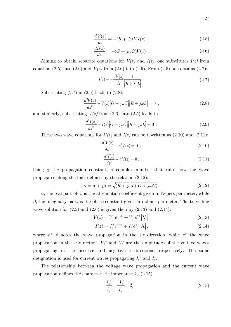
(2.6) as two coupled first-order differential equations:
27
( )( ) ( )
dV zR j L I z
dz , (2.5)
( )( ) ( )
dI zG j C V z
dz . (2.6)
Aiming to obtain separate equations for V(z) and I(z), one substitutes I(z) from
equation (2.5) into (2.6) and V(z) from (2.6) into (2.5). From (2.5) one obtains (2.7):
( ) 1
( )dV z
I zdz R j L
. (2.7)
Substituting (2.7) in (2.6) leads to (2.8):
2
2
( )( ) 0
d V zV z G j C R j L
dz , (2.8)
and similarly, substituting V(z) from (2.6) into (2.5) leads to :
2
2
( )( ) 0
d I zI z G j C R j L
dz . (2.9)
These two wave equations for V(z) and I(z) can be rewritten as (2.10) and (2.11):
2
2
2
( )( ) 0
d V zV z
dz , (2.10)
2
2
2
( )( ) 0
d I zI z
dz , (2.11)
being the propagation constant, a complex number that rules how the wave
propagates along the line, defined by the relation (2.12):
( )( )j R j L G j C . (2.12)
, the real part of , is the attenuation coefficient given in Nepers per meter, while
, the imaginary part, is the phase constant given in radians per meter. The travelling
wave solution for (2.5) and (2.6) is given then by (2.13) and (2.14):
0 0
( ) Vz zV z V e V e , (2.13)
0 0
( ) Az zI z I e I e , (2.14)
where e-z denotes the wave propagation in the +z direction, while ez the wave
propagation in the -z direction. V0+ and V0
- are the amplitudes of the voltage waves
propagating in the positive and negative z directions, respectively. The same
designation is used for current waves propagating I0+ and I0
-.
The relationship between the voltage wave propagation and the current wave
propagation defines the characteristic impedance ZC (2.15):
0 0
0 0
c
V VZ
I I
, (2.15)

28
which can be related to the electrical parameters of the line substituting the general
solution from (2.13) and (2.14) into the transmission line relation in (2.5) and (2.6).
From (2.5) one obtains (2.16):
0 00 0
( )( )
z zz zd V e V e
I e I e R j Ldz
. (2.16)
Solving the derivatives leads to (2.17):
0 0 0 0
( )z z z zV e V e I e I e R j L . (2.17)
Similarly, substituting (2.14) into (2.6) and solving the derivatives one obtains
(2.18):
0 0 0 0
( )z z z zI e I e V e V e G j C . (2.18)
Considering only the forward propagating wave (0 0
0V I ) in equations (2.17)
and (2.18) one obtains (2.19):
0 0
0 0
z z
z z
V e I e R j L
I e V e G j C
, (2.19)
leading to the rewritten for characteristic impedance as (2.20):
0
0
c
V R j LZ
G j CI
. (2.20)
Substituting from (2.12) in (2.20) one obtains (2.21) (IDA, 2015):
[ ]c
R j LZ
G j C
. (2.21)
The same relation for the characteristic impedance can be found by considering
only the backward propagating wave (V0+=I0
+=0).
The current wave propagation (2.14) can be rewritten as (2.22):
0 0( ) z z
c c
V VI z e e
Z Z
. (2.22)
The wavelength on the line is related with the phase constant as (2.23):
2
, (2.23)
and the phase velocity is given by the relation (2.24)
pv f
. (2.24)
Another parameter commonly used is the electrical length of the line, given by z
in radians (IDA, 2015).

29
2.1.2 The Load Reflection Coefficient
Considering a load connected to a transmission line and located at l=0 (l equal to
the maximum z or the length of the line) as shown in Figure 2:
Figure 2 - Transmission line terminated in a load impedance ZL (POZAR, 2005).
Recalling the definition of ZC in (2.15) and, the load impedance will be given by
the relation between the total voltage and current propagating through a transmission
line as (2.25):
(0)(0) / /L c
c c
V V V V V V VZ Z
I I I V Z V Z V V
, (2.25)
being the total voltage and current the sum of the forward and backward propagating
waves. At the condition of matching between load and line, there will not exist a
backward propagating wave (V-=0) since the load impedance equals to the
characteristic impedance of the line.
Therefore, the backward propagating wave will only exist when ZL¹ZC, due to the
reflection of the forward propagating wave at the load. The relation between reflection
V- and forward V+ waves defines the load reflection coefficient as (2.26):
jL cL L
L c
Z ZVe
Z ZV
, (2.26)
being a complex number where G is the phase angle of the reflection coefficient.
2.1.3 Line Impedance and the Generalized Reflection Coefficient
Line impedance refers to the impedance at any point on the line. It can be obtained
dividing the total voltage at any point on the line (2.13) by the total current also at

30
any point on the line (2.14). Rewriting the current in terms of voltage and characteristic
impedance and using the concept of load reflection coefficient presented in (2.26) leads
to (2.27) and (2.28)
( ) ( ) Vl lL
V l V e e , (2.27)
0
( ) ( ) Al lL
VI l e e
Z
. (2.28)
Dividing V(l) by I(l) to obtain the line impedance at any point Z(l) one obtains
(2.29)
( )( )
( ) [ ]( ) ( )
l lL
c l lL
e eV lZ l Z
I l e e
. (2.29)
Using the identities (el+e-l)/2=coshl and (el-e-l)/2=sinhl, the line impedance
equation can also be rearranged as (2.30)
0
0
tanh( )
tanhL c
c
Z Z lZ l Z
Z Z l
. (2.30)
Thus, the reflection coefficient at point l on the line can be achieved by (2.31)
2( )( )
( )
l llL L
Ll l
V e eV ll e
V l V e e
, (2.31)
which can be rewritten as (2.32)
2 2 2( ) l l j lL L
l e e e e . (2.32)
To distinguish it from the load reflection coefficient GL, G(l) is called the generalized
reflection coefficient (IDA, 2015). On a general lossy line this coefficient has an
amplitude |GL| at the load which decays exponentially as z increases (toward the
generator), and a phase varying linearly along l set by the phase constant as (2.33)
( )
2 radl
l . (2.33)
2.1.4 The Terminated Lossless Transmission Line
Considering a lossless line (=0 and =j), terminated in ZL, the voltage and
current on the line becomes (2.34) and (2.35) respectively
( ) ( ) Vj l j lL
V l V e e , (2.34)
0
( ) ( ) Aj l j lL
VI l e e
Z
. (2.35)

31
From (2.30) and using the identity tanh(jl)=j tan(l), the line impedance of a
lossless transmission line is given by (2.36)
Ωtan cos sin
( ) =tan cos sin
L c L cc c
c L c L
Z jZ l Z l jZ lZ l Z Z
Z jZ l Z l jZ l
, (2.36)
and the generalized reflection coefficient by (2.37)
2 2( ) cos 2 sin 2jj l j lL L L
l e e e l j l . (2.37)
The phase rules how the voltage and current vary along the line, resulting in
maxima and minima points, as well for the reflection coefficient. Rearranging the terms
in (2.34) and (2.35) one obtains the maximum and minimum values for voltage (2.38)
max
min
1 ( ) V
1 ( ) V
V V l
V V l
, (2.38)
and for current (2.39)
maxmax
minmin
1 ( ) A
1 ( ) A
c c
c c
VVI l
Z Z
VVI l
Z Z
. (2.39)
A mismatched load implies a not full power transfer from the generator to the load.
This “loss” is called return loss (RL) (POZAR, 2005), defined in dB by (2.40)
20 log dBRL . (2.40)
When there is no reflection (0 matched load), the return loss is equal to ¥ dB,
whereas total reflection (||1) gives a return loss of 0 dB.
Another term used in microwave circuit analysis is called standing wave ratio
(SWR), defined as the ratio between the maximum and minimum voltage (or current)
as (2.41)
max max
min min
1 ( )SWR dimensionless
1 ( )
lV I
V I l
. (2.41)
The SWR is dimensionless and varies between 1 (no reflection) and ¥ (total
reflection).
Rewriting the equations (2.34) and (2.35) for the voltage and current anywhere on
the line, but now expanding the term L one obtains (2.42) and (2.43)
2 2( ) (1 ) (1 ) Vjj l j l j l j lL L
V l V e e V e e e , (2.42)
2 2
0 0
( ) (1 ) (1 ) Ajj l j l j l j lL L
V VI l e e e e e
Z Z
. (2.43)

32
At the load, voltage and current are given by setting l = 0 as (2.44)
0
(1 ) V
(1 ) A
j
L L
j
L L
V V e
VI e
Z
. (2.44)
Analyzing equations (2.42) and (2.43), voltage wave assumes minimum values at
the phase (2.45)
2 (2 1) , 0,1,2,...l n n . (2.45)
Thus, using the identity 2p/, the locations for minimum values of voltage can
be obtained by the relation (2.46)
λmin
( (2 1) ) , 0,1,2,...4
l n n
, (2.46)
which indicates the distance in units of wavelength. Maximum values occur at a
distance of /4 on each side from minimum locations as (2.47)
λmax
( 2 ) , 0,1,2,...4
l n n
. (2.47)
Figure 3 shows the representation of maxima and minima values for voltage and
current standing waves along the line.
Figure 3 - Locations of maximum and minimum standing wave values along the line toward the
generator (IDA, 2015).
Line impedance assumes maximum values at locations of voltage maxima (current
minima), and minimum ones at locations of voltage minima (current maxima).
33
2.1.5 Transmission Line Transfer Function
The transfer function of a transmission line ideally terminated in ZC is defined by
the relation (2.48) (ROHLING, 2011):
d d j dH e e e , (2.48)
with d representing the total length of the line under analysis.
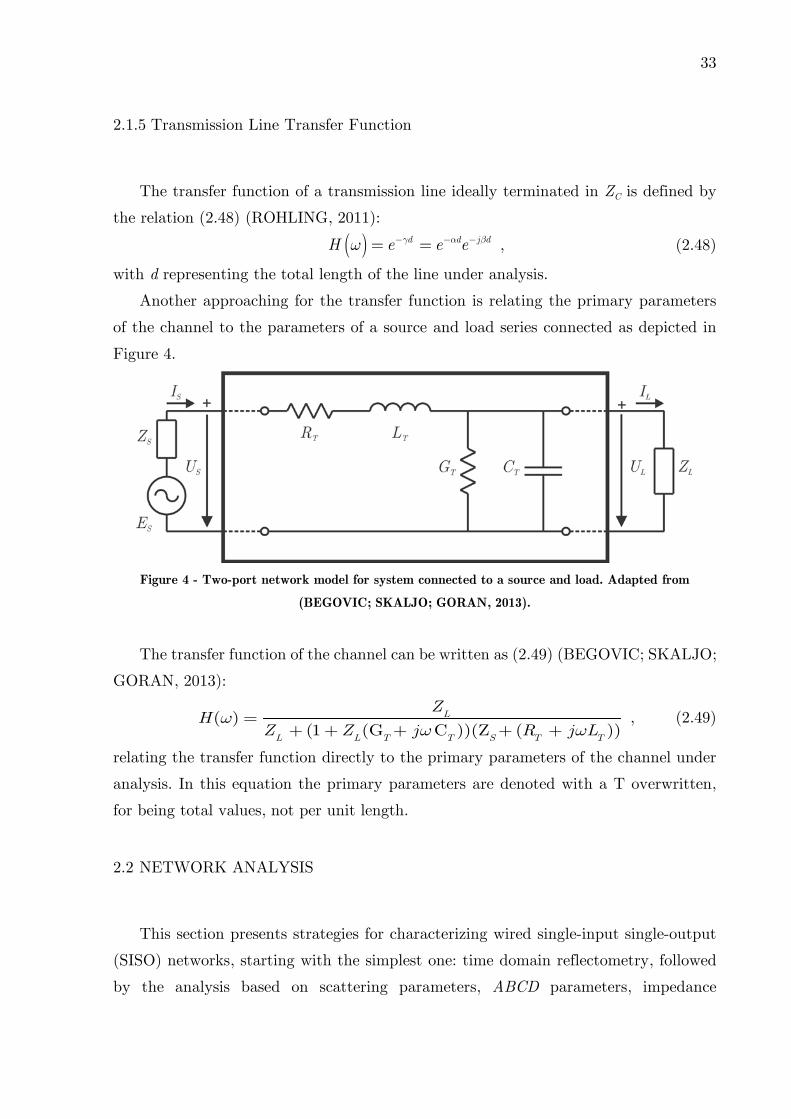
Another approaching for the transfer function is relating the primary parameters
of the channel to the parameters of a source and load series connected as depicted in
Figure 4.
Figure 4 - Two-port network model for system connected to a source and load. Adapted from
(BEGOVIC; SKALJO; GORAN, 2013).
The transfer function of the channel can be written as (2.49) (BEGOVIC; SKALJO;
GORAN, 2013):
( )(1 (G C ))(Z ( ))
L
L L T T S T T
ZH
Z Z j R j L
, (2.49)
relating the transfer function directly to the primary parameters of the channel under
analysis. In this equation the primary parameters are denoted with a T overwritten,
for being total values, not per unit length.
2.2 NETWORK ANALYSIS
This section presents strategies for characterizing wired single-input single-output
(SISO) networks, starting with the simplest one: time domain reflectometry, followed
by the analysis based on scattering parameters, ABCD parameters, impedance
34
spectroscopy and finally a channel model for linear time invariant channels aiming to
accomplish the Shannon’s capacity.
2.2.1 Time Domain Reflectometry
Time domain reflectometry (TDR) is a method introduced in the early 1960’s for
evaluating a transmission line in time domain using a pulse generator and a broadband
oscilloscope. It consists in applying a high frequency stimulus over the channel (impulse
or step) and monitoring the reflected signals caused by impedance mismatches along
the line, as well as by the end of the line. Magnitude of each reflection is directly related
to the reflection coefficient related to the pulse generator impedance, while its location
in time gives the exact location of that mismatch in the line. Once known the line
propagation velocity it is possible to associate the time of each reflection gave by the
TDR trace with its location in the line. The type of each discontinuity can also be
identified by its response, being capacitive or inductive (AGILENT TECHNOLOGIES,
2012). Changes in impedance can be caused by faults as short-circuits, splices, open
connections, taps in the cable system, deteriorated neutrals, water ingress into
insulation material or joints, and high resistance connectors (HERNANDEZ-MEJIA,
2016). Compared to other measurement techniques, time domain reflectometry
provides a more intuitive and direct look at the channel under analysis (AGILENT
TECHNOLOGIES, 2013), it is easy to employ, test equipment are small and not
expensive, analysis at low voltage and periodic testing provides historical data.
The magnitude of the reflections () will be given by the relation between the
characteristic impedance of the line ZC and the characteristic impedance of local
discontinuity Zd as (2.50):
d c
d c
Z Z
Z Z
. (2.50)
The reflection coefficient varies from -1, meaning short circuit, to 1, meaning open
circuit. The zero value represents no reflection, implying the perfect matching.
The location of each mismatch in unit of length is achieved by the relation between
the time taken to the pulse travel to this location, reflect and travel back to the start
of the line as (2.51):
2p
m
v tD , (2.51)
35
being t the transit time, vp the velocity of propagation and Dm the location of the
mismatch. If unknown yet, the velocity of propagation can be determined using a cable
of the same type of a known length, and verifying the time required for an incident
pulse travel down, reflect at the end of the line in an open circuit termination and
travel back to the start (AGILENT TECHNOLOGIES, 2013). The velocity of
propagation is generally defined in terms of speed of light in vacuum environment, as
100 % reference. For instance, the velocity of propagation on a coaxial line RG-58U is
65.9 % (PASTERNACK, 2017), while for a CAT5e twisted pair line is about 67 %
(DRAKA, 2017).
The characteristics of the pulse are very relevant to the performance of the analysis.
The amplitude is defined as the peak amplitude of the TDR pulse, being the maximum
value of the trace not depending on its shape. The pulse width is defined as the time
that the amplitude keeps at 50 % of its peak amplitude, and is related to the resolution
in time / length of the result TDR trace. The resolution is given by the relation (2.52)
:
Resolution 2
widtht
t . (2.52)
Therefore, a pulse 10 ns wide performs a TDR trace with resolution of 5 ns.
Considering a line with velocity of propagation of 66%, the resolution in length is about
0.99 m. The narrower the pulse the greater the resolution of the analysis.
Despite of the easy implementation, there is an inherited drawback related to
reflectometry based methods known as dead zone or a blind spot. It is generated when
the channel under test is short enough in a way that an overlap occurs between the
incident and the reflected wave from a fault (KWAK et al., 2008). For this reason, this
phenomenon is truly relevant as it indicates the minimum cable length which can be
tested. The blind spot length is directly related to the width of the incident pulse. The
wider the pulse the larger the blind spot. The blind spot length LB is equal to the
resolution time converted into length once it is known the velocity of propagation in
the cable as (2.53) :
2
p widthB
v tL . (2.53)
So, taking for instance the example described above where the pulse is 10 ns wide,
the blind spot is 0.99 meter long. Faults located below this length will not be possible
to be identified using the TDR trace. There are some solutions to work around this
problem like the addition of an extension cable as the simplest one, the dual time base

36
technique (WALSH, 1995) and reduction of the blind spot using signal processing
techniques (KWAK et al., 2008). Another approach is applying the method from both
perspectives, in other words, applying the pulse and monitoring the reflections from
port one and also from port two, enabling the reading of both ends of the channel under
test once the blind spot of the first perspective will be the end of the line on the second
one.
Another problem related to the TDR method is given by the attenuation that the
pulse will suffer while traveling along the line, being a function of the distance traveled.
Losses in the bulk insulation and propagation through the resistance of the channel
components induce energy loss of an incident pulse (HERNANDEZ-MEJIA, 2016).
TDR pulses with narrow width, composed by high frequency components, suffer higher
attenuation than the wider ones, with low frequency components. Attenuation increases
with frequency and for long channels the pulses can attenuate until reach the noise
background level, hiding the reflections information. In addition to the attenuation,
the TDR pulse suffers also dispersion and distortion. Different frequency components
travel along the channel at different speeds, causing a phase shift of each frequency
component of the TDR pulse, being a function of the distance traveled by the pulse
and its frequency components profile (HERNANDEZ-MEJIA, 2016). Both distortions
attenuation and dispersion can occur simultaneously, affecting the accuracy of locating
impedance mismatches along the channel.
There is a tradeoff when specifying the pulse width and amplitude to apply the
TDR method. Both affect the TDR resolution, in other words the ability to identify
all those impedance mismatches along the channel under test. Having a good amplitude
resolution means that even small changes in the reflection coefficient can be identified
over the TDR trace, in a way that all the reflection coefficients of the channel will be
represented by an amplitude higher than the background noise. So, the amplitude
resolution is directly linked to the distance that the incident pulse or reflection is able
to travel without reaching the noise level amplitude. In other hand, the time resolution
is referred to the ability to distinguish two impedance mismatches locations closely
spaced. The wider the pulse, the harder to recognize them. The tradeoff between the
amplitude and time resolution is all based on attenuation and dispersion. Improving
time resolution by using a narrower pulse may compromise the amplitude resolution,
as well as improving the amplitude resolution using wider pulse may compromise the
time resolution. Therefore, there is an optimal point when choosing amplitude and
width of the TDR pulse.
37
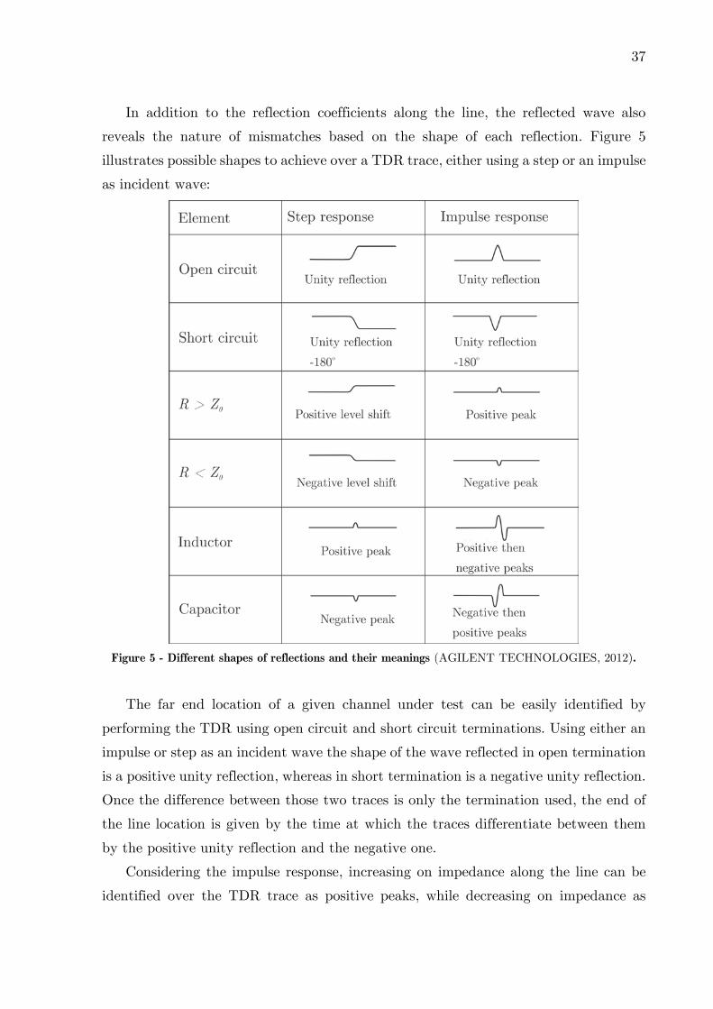
In addition to the reflection coefficients along the line, the reflected wave also
reveals the nature of mismatches based on the shape of each reflection. Figure 5
illustrates possible shapes to achieve over a TDR trace, either using a step or an impulse
as incident wave:
Figure 5 - Different shapes of reflections and their meanings (AGILENT TECHNOLOGIES, 2012).
The far end location of a given channel under test can be easily identified by
performing the TDR using open circuit and short circuit terminations. Using either an
impulse or step as an incident wave the shape of the wave reflected in open termination
is a positive unity reflection, whereas in short termination is a negative unity reflection.
Once the difference between those two traces is only the termination used, the end of
the line location is given by the time at which the traces differentiate between them
by the positive unity reflection and the negative one.
Considering the impulse response, increasing on impedance along the line can be
identified over the TDR trace as positive peaks, while decreasing on impedance as

38
negative peaks. Inductance characteristics are revealed by positive followed by negative
peaks, while locations with capacitance characteristics the contrary.
As described, time domain reflectometry method requires ideal open and short
circuit terminations, which are difficult to achieve over a broadband frequency range.
Moreover, open circuit terminations cause stray capacitance due to electric field
fringing at high frequencies, while short circuit terminations introduce additional
inductance (PAPAZYAN et al., 2004).
2.2.2 Scattering Parameters
Scattering parameters are widely used for characterizing n-port networks. These
parameters relate travelling waves to the network behavior, rather than voltages and
currents. The waves scattered or reflected from the network are related to those waves
incident upon the network (AGILENT TECHNOLOGIES, 2006). From them it is
possible to extract the characteristic impedance, propagation constant and the
distributed parameters (resistance, inductance, conductance and capacitance) as well
of the line (PAPAZYAN et al., 2004).
The scattering matrix S represents the relationship between the normalized incident
voltage waves [V +] and the normalized reflected ones [V -] as (2.54):
V S V , (2.54)
which can be detailed as (2.55):
1 111 12 1
21 22 22 2
2
.
j
j
ij j iji j
V VS S S
S S SV V
S S SV V
. (2.55)
Each element of the scattering matrix describes the electrical behavior related to
two specific ports of the network under analysis. The parameter Sij relates the reflected
wave from port i to the incident wave from port j as (2.56):
iij
j
VS
V
. (2.56)
Rather than short or open circuit terminations as demanded in methods for
characterizing based on the reflectometry principle, the extraction of the scattering
parameters is made by terminating one or the other port with the normalizing
impedance Z0 of the network analyzer equipment, which is normally 50 . For a given

39
2-port network, there will exist four scattering parameters, and the topology for
acquiring them is shown in Figure 6.
V1+
V1-
S11 S12
S21 S22
V2+
V2-
Z0
Z0~
Figure 6 - Scattering parameters measurement topology for 2-port network.
And its S matrix is given by (2.57):
2 11 12 2
21 221 1
V S S V
S SV V
, (2.57)
being S11 the input reflection coefficient with matched output, S21 the forward
transmission coefficient with matched output, S22 the output reflection coefficient with
matched input, and S12 the reverse transmission coefficient with matched input
(AGILENT TECHNOLOGIES, 2006). Therefore, the parameters S11 and S22 are related
with how matched is the network referenced to Z0, whereas S12 and S21 are related to
how the network attenuates or amplifies an input signal.
When a network has the same transmission and reflection characteristics from port
one to port two in comparison to the contrary perspective, it is designated as a
reciprocal network (AGILENT TECHNOLOGIES, 2006). The S-parameter matrix of
this kind of network is equal to its transpose, implying S11=S22 and S12=S21.
The scattering parameters can also be written in terms of transmission line wave
propagation characteristics as (2.58) (PAPAZYAN et al., 2004)
2 2
0 02 2
0 0
( )sinh 212 ( )sinh
C C
C CS
Z Z l Z ZS
Z Z Z Z lD
, (2.58)
being DS = 2ZCZ0 cosh l + (ZC2+Z0
2) sinh l and l the line length.
Assuming that the line is reciprocal (S11ºS22 and S21ºS12), the propagation constant
can be derived from (2.58), written in function of these parameters as (2.59)
2 2
1 11 21
21
11( ) cosh
2
S S
l S
, (2.59)
as well the characteristic impedance ZC as (2.60)
2 211 21
0 2 211 21
1( )
1C
S SZ Z
S S
. (2.60)

40
The distributed parameters can be deduced from the definition of propagation
constant (2.12) and characteristic impedance (2.21) as (2.61)
( ) Re
( ) Im /
( ) Re /
( ) Im / /
C
C
C
C
R Z
L Z
G Z
C Z
. (2.61)
2.2.2.1 Scattering parameters in time domain
Scattering parameters can be converted to time domain to provide an impedance
profile and impulse response of the line under test. As seen in section 2.2.1,
reflectometry based methods enable to find physically faults and impedance mismatches
along the line, which is also possible to achieve from the analysis of the parameter S11
converted to time domain. Whereas, time domain transmission analysis give the
impulse response of the line, equivalent to the integral of the parameter S21 converted
to time domain. The conversion is achieved by mathematical tools that enable the
change on the analysis scenario from frequency to time domain, and vice-versa. One
conversion method usually performed by a number of commercial Network Analyzers
is the Inverse Chirp Z Transform, but before to explain it, one must to define the direct
Chirp Z Transform. Proposed by Lawrence Rabiner in 1969, the Chirp Z Transform
consists in an algorithm that evaluates the Z transform of a sequence of N samples at
M points in the Z plane, standing either right on circular or spiral contours beginning
at any arbitrary point (RABINER; SCHAFER; RADER, 1969). The Chirp Z
Transform of sequence {x(n)} with 0 n < N-1 is defined as (2.62)
1
0
( )N n
kCZT
n
X k x n A W
, (2.62)
being X(k) the resulting M points sequence defined in 0 k < M-1 and, ACZT and W
arbitrary complex numbers defined by (2.63) and (2.64)
02
0
j
CZTA Ae , (2.63)
02
0
jW W e . (2.64)
ACZT is the starting point for the sweeping in Z plane, and W defines how the
contour spirals over the plane. A0 and 0 are the starting radius and angle respectively,
and 0 the angle step size. W0 sets the rate at which the contour spirals in (greater
than 1) or out (less than 1) from a circle of radius A0. Therefore, the contour at which

41
the Chirp Z transform is defined in the Z plane, shown in Figure 7, is set by the term
ACZTW-k.
Figure 7 - Chirp Z Transform: spiral contour in the Z plane. Adapted from (RABINER; SCHAFER;
RADER, 1969).
From this definition, Discrete Fourier Transform can be interpreted as a specific
case of the Chirp Z Transform for being restricted to the unit circle in the z plane.
Among the advantages provided by the Chirp Z Transform, one can list: the output
sampling can be different from the input one (N¹M or N=M); both N and M can be
prime numbers; arbitrary frequency resolution given by arbitrary angular spacing along
the contour; random starting point of analysis in the Z plane, enabling narrow-band
analysis.
The analysis of the scattering parameters in time domain requires the solution for
the inverse problem, performed by the Inverse Chirp Z Transform (ICZT). Mersereau
has developed an algorithm to calculate the Inverse Chirp Z Transform through the
relation ICZT(X(k)) = ACZTnCZT(1,W -1,CkX(k),N), with Ck a calculated coefficients
array (MERSEREAU, 1974). Although, even the author mentions that the number of
problems to which the proposed algorithm might be applied is extremely sensitive to
quantization errors. Frickey has proposed that the inverse transform can be
accomplished by ICZT(X(k)) = [CZT(X(k)*)]*, but the performance is only guaranteed
for the CZT operating at or inside the unit circle in the Z plane (FRICKEY, 1994).
Another approach is presented by Yague et al., following a direct method as (2.65):
1 1
12 ( )( )
10
1( ) ( )
0,1,..., 1
Mj f k f t n t
k
x t n t X k eM
n N
, (2.65)
42
being the data in time domain denoted by x(t1+nt), start frequency and time by f1
and t1 respectively, the step frequency and time by f and t respectively (DE
PORRATA-DORIA I YAGUE; IBARS; MARTINEZ, 1998).
Although the arbitrariness of CZT in choosing the number of input and output
samples is considered an advantage, it can also bring matters to the inverse problem
scenario. The difference between the sampling set in frequency and in time can render
unstable inversion due to ill-posedness of the problem.
2.2.3 ABCD Matrix
The ABCD Matrix (or Transmission Matrix) is another method to characterize a
two-port network, which defines four variables that relate total voltage and current in
each port as (2.66):
1 2 2
1 2 2ABCD
V AV BI
I C V DI
. (2.66)
Rewriting (2.66) in matrix form leads to (2.67):
1 2
1 2ABCD
V A B V
I C D I
. (2.67)
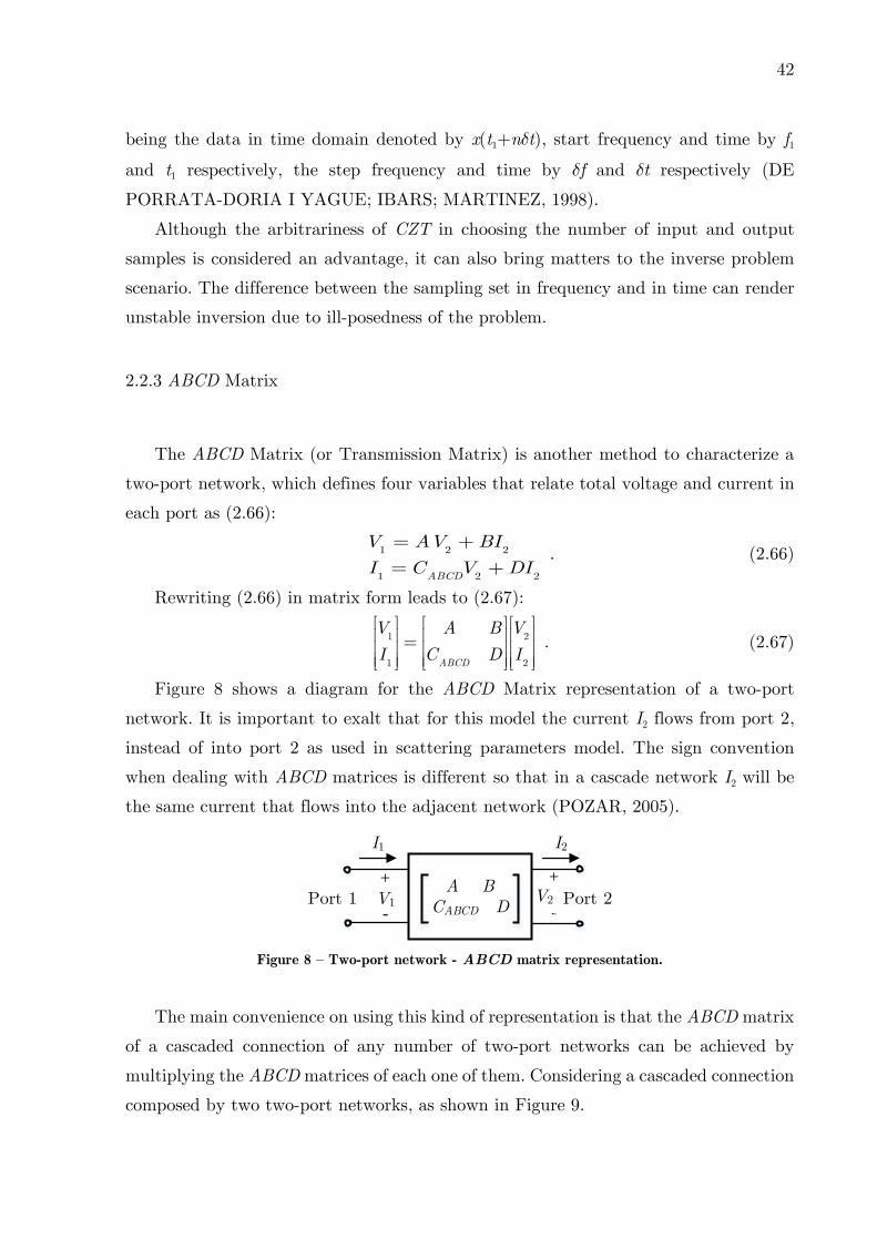
Figure 8 shows a diagram for the ABCD Matrix representation of a two-port
network. It is important to exalt that for this model the current I2 flows from port 2,
instead of into port 2 as used in scattering parameters model. The sign convention
when dealing with ABCD matrices is different so that in a cascade network I2 will be
the same current that flows into the adjacent network (POZAR, 2005).
V2V1-
A BCABCD D
+
-
+
I2I1
Port 1 Port 2
Figure 8 – Two-port network - ABCD matrix representation.
The main convenience on using this kind of representation is that the ABCD matrix
of a cascaded connection of any number of two-port networks can be achieved by
multiplying the ABCD matrices of each one of them. Considering a cascaded connection
composed by two two-port networks, as shown in Figure 9.

43
A2 B2
C2 D2V3-
+
I3
V1-
A1 B1
C1 D1
+V2-
+
I2I1
Figure 9 - Two-port networks in cascaded connection.
The ABCD matrix for the individuals two-ports is given by (2.68) and (2.69):
1 1 1 2
1 1 1 2
V A B V
I C D I
, (2.68)
2 2 2 3
2 2 2 3
V A B V
I C D I
. (2.69)
Substituting (2.69) in (2.68) leads to (2.70):
1 1 1 2 2 3
1 1 1 2 2 3
V A B A B V
I C D C D I
, (2.70)
which is equal to the product of the individual ABCD matrices. One must exalt that
the order of multiplication of the matrices must be the same as the networks are
arranged.
The ABCD parameters can also be related to the secondary parameters of a
reciprocal transmission line characteristic impedance and propagation constant
(LAMPE; TONELLO; SWART, 2016), defined by (2.71):
1 2
cosh( )
sinh( )
sinh( )C
ABCD C C
A D d
B Z d
C Z d BZ
, (2.71)
with the total line length denoted by d. Rewriting the ABCD parameters in matrix
notation one obtains (2.72):
1
cosh( ) sinh( )
sinh( ) cosh( )c
ABCD c
d Z dA B
C D Z d d
. (2.72)
Then one can relate those parameters to the input impedance of a set composed by
a given transmission line terminated in a load impedance ZL as (2.73):
cosh sinh
cosh sinhL c L
in cc L ABCD L
Z d Z d AZ BZ Z
Z d Z d C Z D
. (2.73)
Now considering the channel plus load set connected to a source with impedance
ZS. Its transfer function can be written in function of those ABCD parameters as (2.74)
(FRANCIS; TITUS, 2011):
44
( ) L
L ABCD S L S
ZH f
AZ B C Z Z DZ
. (2.74)
2.2.4 Impedance Spectroscopy
The impedance spectroscopy method consists in measuring impedance of a
particular material under test over a given frequency spectrum, which enables the
analysis of the changes of electrical properties in each frequency. The principle of this
method is relating the input impedance measured at each frequency to the
characteristic impedance and to the propagation constant of the line under test.
Considering a transmission line terminated in short circuit (ZL=0), the input impedance
presented in equation (2.30) becomes (2.75):
tanh( )short c
Z Z d , (2.75)
with the total line length denoted by d. Using the same logic, but now considering an
open circuit as termination (ZL®¥) the input impedance will be (2.76):
/ tanh( )open c
Z Z d . (2.76)
Through the relations between the definition of (2.12), impedance for short circuit
as load (2.75) and impedance for open load (2.76), one can obtain expressions for the
characteristic impedance (2.77) and propagation constant (2.78) (QINGHAI SHI;
TROLTZSCH; KANOUN, 2011):
c short open
Z Z Z , (2.77)
short
open
Z
Z . (2.78)
Then, the distributed parameters can be extracted following the same relations
presented in equations (2.61).
2.2.5 Shannon-Hartley Theorem
Shannon-Hartley theorem states that the theoretical tightest upper bound on the
information rate of data that can be performed at a communication system operating
at a bandwidth BW (Hz) using an average signal power S (W) through a channel
subject to additive white Gaussian noise power level N (W) is given by (2.79)
(SHANNON, 1948):
45
max 2
log 1S
C BWN
= +
, (2.79)
being the channel capacity represented by Cmax (bps), and signal-to-noise ratio (SNR)
designed by the relation between the communication signal to the noise at the receiver,
as a linear power ratio.
A Gaussian noise is defined as a filtered thermal noise, with power spectrum N(f).
For a channel perturbed by any Gaussian noise, channel capacity can be written as
frequency dependent function, dividing the band into a large number of small bands,
with N(f) approximately constant in each. The total capacity for a given distribution
S(f) can be written as (2.80) (SHANNON, 1949):
max 20
( )log 1
(f)
BW S fC df
N
= +
∫ . (2.80)
2.2.6 LTI Channel Model
A Linear Time Invariant channel is defined as the channel which has constant
frequency response H(f) over time. In other words, the electrical characteristics of the
channel do not vary over time. For instance, wireless channels are commonly treated
as time variant since the electrical properties of the medium cannot be assumed
constant, while the wired ones are treated as time invariant since the immunity to
external elements.
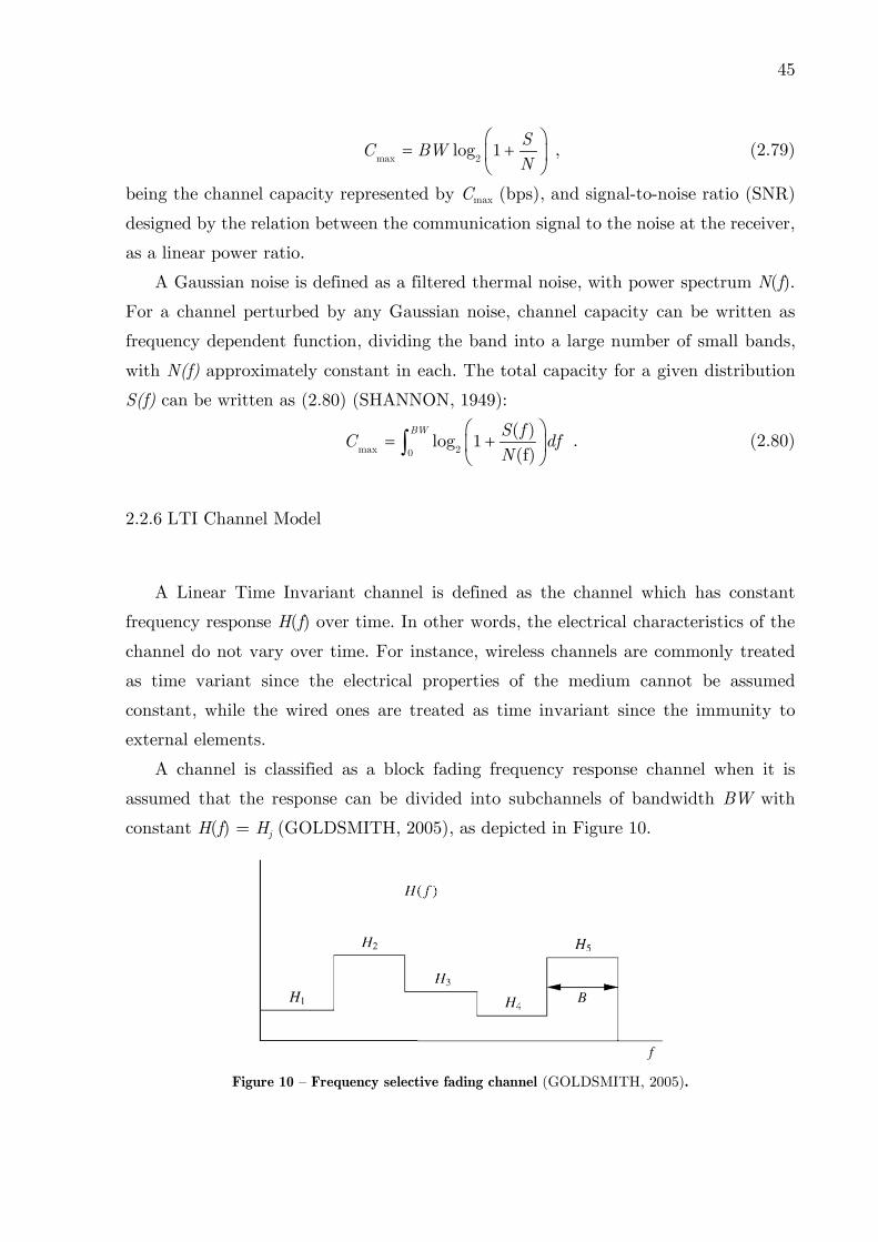
A channel is classified as a block fading frequency response channel when it is
assumed that the response can be divided into subchannels of bandwidth BW with
constant H(f) = Hj (GOLDSMITH, 2005), as depicted in Figure 10.
Figure 10 – Frequency selective fading channel (GOLDSMITH, 2005).
46
This channel is composed then by a set of AWGN channels in parallel with SNR
|Hj|2 Pj / N0BW on the jth channel, with power allocated Pj to the jth channel. So the
total capacity of the channel is the sum of rates on each subchannel as (2.81):
2
max 2max : 0
log 1j j j
j j
P P P
H PC BW
N BW
. (2.81)
2.3 ORTHOGONAL FREQUENCY DIVISION MULTIPLEXING
Orthogonal Frequency Division Multiplexing (OFDM) is a promising multicarrier
modulation technique for PLC applications, presenting high spectral efficiency and
properties that mitigate the harsh characteristics of power line channels
(KOTCHASARN, 2017). Its principle consists in splitting a high rate data stream into
a number of lower rate streams and transmit them simultaneously over a number of
orthogonal subcarriers, which ensures the non-interference between them. The
orthogonality property can be lost due to multipath or non-stationary behavior of the
channel, causing intersymbol interference (ISI). The phenomenon drastically degrades
the received signal, being one of the major obstacles that high data rate systems must
overcome (RAHMAN; MAJUMDER, 2014). However, ISI can be avoided completely
or can be reduced at least considerably by a proper choice of OFDM system parameters
(ROHLING, 2011).
Essentially the transmission process involves assembling the input information into
N blocks ofcomplex numbers, one for each sub-channel. Then, an Inverse Fast Fourier
Transform (IFFT) is performed on each block, resulting in N separate QAM signal
with spectrum shaped as sinc function, with nulls at the center of the other sub-carriers
(BAHAI; SALTZBERG; ERGEN, 2004). The resultant signal is transmitted serially
over the channel. At the receiver, the information is recovered by performing an FFT
on the received block of signal samples. A simple block diagram of an OFDM system
is presented in Figure 11.

47
Figure 11 - Block diagram of basic OFDM system. Adapted from (BAHAI; SALTZBERG; ERGEN,
2004).
To avoid overlap of consecutive transmitted blocks, a short cyclic prefix on the
transmit signal is used, acting as a buffer between blocks (LIN; PHOONG;
VAIDYANATHAN, 2011). This feature allows perfect distortionless data recovery at
the transmitter, even for dispersive channels. However, prefixing leads to an increasing
on the use of bandwidth.
OFDM characteristics enable transmission over extremely hostile channel at a
comparable low complexity with high data rates, and because of them this modulation
technique has been adopted in important wireless communication systems such as
Digital Audio Broadcasting (DAB), Digital Video Broadcasting (DVB), Wireless Local
Area Network (WLAN), Wireless Metropolitan Area Network (WMAN), and Multi
Band – OFDM Ultra Wide Band Besides. OFDM is also employed in wired applications
such as Asymmetric Digital Subscriber Line (ADSL) and Power Line Communication
(PLC) (RAHMAN; MAJUMDER, 2014).
2.3.1 Power Line Communication
Power Line Communication (PLC) is the name given to the technology with the
purpose of implementing data transmission over existed structures already used on
energy distribution. The transmission occurs through modulation in high frequency

48
signals, going from hundreds of Hertz to hundreds of Mega Hertz (LAMPE;
TONELLO; SWART, 2016). Its nature is intrinsic to the fact that the physical medium
used for transmission is inserted in harsh environments considering electromagnetic
interference, as well as channel parameters such as nominal noise, impedance and
attenuation.
The PLC technology uses DFT-based transceivers. This is related to the
modulation technique employed. For wired DSL (Digital Subscriber Line) applications
it is designated as a DMT (Discrete Multitone) based system, whereas for wireless local
area networks and broadcasting applications as OFDM (Orthogonal Frequency
Division Multiplexing) based system (LIN; PHOONG; VAIDYANATHAN, 2011).
In DMT based systems, signals are transmitted over copper lines, which implies
that the channel characteristics do not vary constantly. This feature enables power
allocation over the subcarriers considering the channel state information evaluated by
the system, allowing the exploitation of the disparity among the subchannel noise
variances for a bit rate maximization (LIN; PHOONG; VAIDYANATHAN, 2011). In
OFDM systems, there is no such constancy on channel behavior, so the transceiver
operates independently and, therefore, with no power allocation. That is the reason
why OFDM appears as a very useful modulation technique for broadcasting
applications, where there are many receivers operating at the same transmission paths.
2.3.1.1 HomePlug AV2
The reuse of existing wires to deploy wide band services has attracting industry
and research communities to dedicate attention to in-home power line communication.
In 2001 HomePlug Alliance, an industry-led organization, created a set of specifications
within the scope of power line networking, first named HomePlug 1.01. Then, in 2005
it was released a second version under the name HomePlug AV (ALLIANCE;
RESERVED, 2005). The AV acronym abbreviates “Audio,Video”, refereeing to its
data streaming application. HomePlug AV provides 200 Mbps class power line
networking capability through PHY (Physical layer) and MAC (Media Access Control)
technologies (YONGE et al., 2013). PHY layer operates in the frequency range of 2-28
MHz, using windowed OFDM and a powerful Turbo Convolutional Code (TCC) that
provides robust performance within 0.5 dB of Shannon’s limit. OFDM operates into
917 carriers with a flexible guard interval. 1024 QAM (Quadrature Amplitude
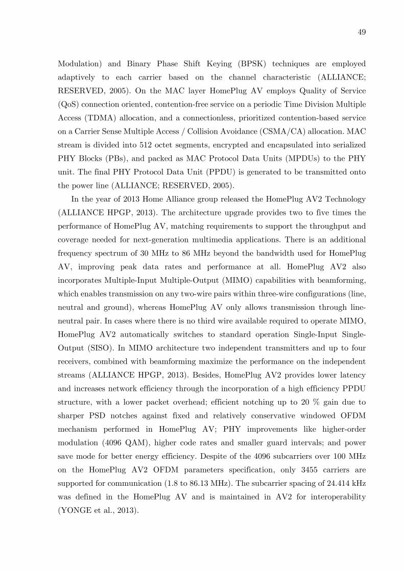
49
Modulation) and Binary Phase Shift Keying (BPSK) techniques are employed
adaptively to each carrier based on the channel characteristic (ALLIANCE;
RESERVED, 2005). On the MAC layer HomePlug AV employs Quality of Service
(QoS) connection oriented, contention-free service on a periodic Time Division Multiple
Access (TDMA) allocation, and a connectionless, prioritized contention-based service
on a Carrier Sense Multiple Access / Collision Avoidance (CSMA/CA) allocation. MAC
stream is divided into 512 octet segments, encrypted and encapsulated into serialized
PHY Blocks (PBs), and packed as MAC Protocol Data Units (MPDUs) to the PHY
unit. The final PHY Protocol Data Unit (PPDU) is generated to be transmitted onto
the power line (ALLIANCE; RESERVED, 2005).
In the year of 2013 Home Alliance group released the HomePlug AV2 Technology
(ALLIANCE HPGP, 2013). The architecture upgrade provides two to five times the
performance of HomePlug AV, matching requirements to support the throughput and
coverage needed for next-generation multimedia applications. There is an additional
frequency spectrum of 30 MHz to 86 MHz beyond the bandwidth used for HomePlug
AV, improving peak data rates and performance at all. HomePlug AV2 also
incorporates Multiple-Input Multiple-Output (MIMO) capabilities with beamforming,
which enables transmission on any two-wire pairs within three-wire configurations (line,
neutral and ground), whereas HomePlug AV only allows transmission through line-
neutral pair. In cases where there is no third wire available required to operate MIMO,
HomePlug AV2 automatically switches to standard operation Single-Input Single-
Output (SISO). In MIMO architecture two independent transmitters and up to four
receivers, combined with beamforming maximize the performance on the independent
streams (ALLIANCE HPGP, 2013). Besides, HomePlug AV2 provides lower latency
and increases network efficiency through the incorporation of a high efficiency PPDU
structure, with a lower packet overhead; efficient notching up to 20 % gain due to
sharper PSD notches against fixed and relatively conservative windowed OFDM
mechanism performed in HomePlug AV; PHY improvements like higher-order
modulation (4096 QAM), higher code rates and smaller guard intervals; and power
save mode for better energy efficiency. Despite of the 4096 subcarriers over 100 MHz
on the HomePlug AV2 OFDM parameters specification, only 3455 carriers are
supported for communication (1.8 to 86.13 MHz). The subcarrier spacing of 24.414 kHz
was defined in the HomePlug AV and is maintained in AV2 for interoperability
(YONGE et al., 2013).

50
3 METHODOLOGY
Aiming to explore the means to characterize a channel, two different experimental
sets are proposed. The first one aims to investigate the influence of length over channel
capacity, obtained from scattering parameters following the Shannon Hartley’s
theorem. The capacities are compared to real performance of a communication system
running over the cables as channel. The second set investigates the electrical behavior
of a channel at all, from time domain measurements analysis to frequency domain
measurements analysis.
Both experimental sets exploit frequency analysis bands up to 4 GHz, covering the
following bands defined by the International Telecommunications Union (ITU):
medium frequency (MF: 300 kHz to 3 MHz), high frequency (HF: 3 MHz to 30 MHz),
very high frequency (VHF: 30 MHz to 300 MHz), ultra high frequency (UHF: 300 MHz
to 3 GHz) and a small part of super high frequency (SHF: 3 GHz to 30 GHz).
3.1 INFLUENCE OF THE LENGTH OVER THE CHANNEL CAPACITY SET
Two different kinds of cables were selected to be characterized in a way to obtain
their capacities in function of length and noise level. In addition, the performance of a
communication system is verified using PLC devices running over those cables in
different lengths as the channel. The idea is comparing the capacities in function of
noise level and length curves to the performance obtained for each length set.
The selected cables are an unshielded twisted pair CAT5e and a flexible stranded
two-wire copper 1.5 mm² pair, both starting with 100 meters as initial length,
subsequently decreasing 10 meters in length at each round, until reach only 10 meters.
The experiment consists in extracting the scattering parameters of each cable in each
length set defined. From them it is achieved the frequency response for each length.
Proceeding to the calculus of the channel capacity, curves are fitted from the response
of each length case, considering the following channel response model (3.1) (EZZINE
et al., 2017):
0 1( ) 2( )kfa a f d j fH f e e . (3.1)
The first term composed by an exponential of order –(a0+a1f fk)d denotes the overall
attenuation. The second one of order –j 2pf is the delay of the wave, being the
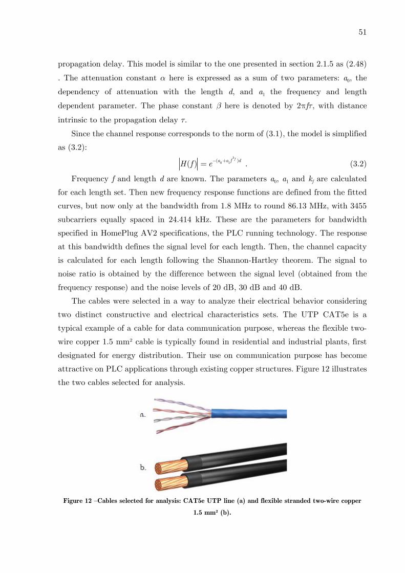
51
propagation delay. This model is similar to the one presented in section 2.1.5 as (2.48)
. The attenuation constant here is expressed as a sum of two parameters: a0, the
dependency of attenuation with the length d, and a1 the frequency and length
dependent parameter. The phase constant here is denoted by 2pf, with distance
intrinsic to the propagation delay .
Since the channel response corresponds to the norm of (3.1), the model is simplified
as (3.2):
0 1( )( )kfa a f dH f e . (3.2)
Frequency f and length d are known. The parameters a0, a1 and kf are calculated
for each length set. Then new frequency response functions are defined from the fitted
curves, but now only at the bandwidth from 1.8 MHz to round 86.13 MHz, with 3455
subcarriers equally spaced in 24.414 kHz. These are the parameters for bandwidth
specified in HomePlug AV2 specifications, the PLC running technology. The response
at this bandwidth defines the signal level for each length. Then, the channel capacity
is calculated for each length following the Shannon-Hartley theorem. The signal to
noise ratio is obtained by the difference between the signal level (obtained from the
frequency response) and the noise levels of 20 dB, 30 dB and 40 dB.
The cables were selected in a way to analyze their electrical behavior considering
two distinct constructive and electrical characteristics sets. The UTP CAT5e is a
typical example of a cable for data communication purpose, whereas the flexible two-
wire copper 1.5 mm² cable is typically found in residential and industrial plants, first
designated for energy distribution. Their use on communication purpose has become
attractive on PLC applications through existing copper structures. Figure 12 illustrates
the two cables selected for analysis.
Figure 12 –Cables selected for analysis: CAT5e UTP line (a) and flexible stranded two-wire copper
1.5 mm² (b).
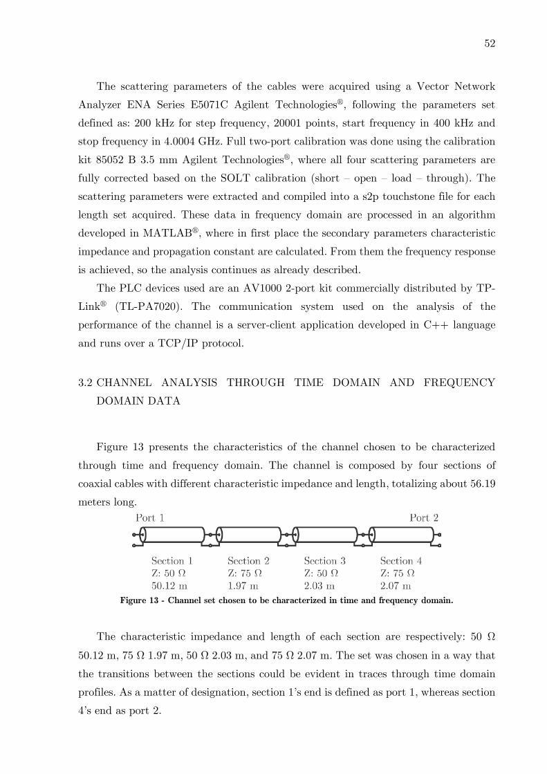
52
The scattering parameters of the cables were acquired using a Vector Network
Analyzer ENA Series E5071C Agilent Technologies®, following the parameters set
defined as: 200 kHz for step frequency, 20001 points, start frequency in 400 kHz and
stop frequency in 4.0004 GHz. Full two-port calibration was done using the calibration
kit 85052 B 3.5 mm Agilent Technologies®, where all four scattering parameters are
fully corrected based on the SOLT calibration (short – open – load – through). The
scattering parameters were extracted and compiled into a s2p touchstone file for each
length set acquired. These data in frequency domain are processed in an algorithm
developed in MATLAB®, where in first place the secondary parameters characteristic
impedance and propagation constant are calculated. From them the frequency response
is achieved, so the analysis continues as already described.
The PLC devices used are an AV1000 2-port kit commercially distributed by TP-
Link® (TL-PA7020). The communication system used on the analysis of the
performance of the channel is a server-client application developed in C++ language
and runs over a TCP/IP protocol.
3.2 CHANNEL ANALYSIS THROUGH TIME DOMAIN AND FREQUENCY
DOMAIN DATA
Figure 13 presents the characteristics of the channel chosen to be characterized
through time and frequency domain. The channel is composed by four sections of
coaxial cables with different characteristic impedance and length, totalizing about 56.19
meters long.
Figure 13 - Channel set chosen to be characterized in time and frequency domain.
The characteristic impedance and length of each section are respectively: 50
50.12 m, 75 1.97 m, 50 2.03 m, and 75 2.07 m. The set was chosen in a way that
the transitions between the sections could be evident in traces through time domain
profiles. As a matter of designation, section 1’s end is defined as port 1, whereas section
4’s end as port 2.
53
3.2.1 Frequency Domain Data Acquisition and Analysis
The scattering parameters of the channel are acquired also using the Vector
Network Analyzer ENA Series E5071C Agilent Technologies®. These data in frequency
domain are processed in an algorithm developed in MATLAB®, where in first place the
secondary parameters (characteristic impedance and propagation constant) are
calculated, and then the primary ones: distributed resistance, inductance, conductance
and capacitance. Also from the secondary ones it is possible to achieve the channel
frequency response, which added to a noise model leads to the Shannon channel
capacity. This completes the whole set of analysis in frequency domain. On other hand,
the analysis of the channel in time domain is made by the conversion of the frequency
domain scattering parameters using the Inverse Chirp Z Transform. Results are the
impulse response, given by the analysis of the parameter S21 in time domain, and the
impedance profile of the channel, given by the parameter S11 in time domain. In
addition, it is proposed a different approach for the conversion to time domain, leaded
by a sparse solution of the problem, which it is detailed explained in the following
subsection 3.2.1.1. Figure 14 illustrates the set of the proposed analysis of the channel.
Figure 14 - Block diagram for the channel analysis proposed.
Before starting the measurements, one must select the frequency parameters set.
Essentially, this selection will define more than just resolution and span for the analysis
in frequency domain, but also the time domain analysis configurations. The maximum
time for sampling is defined by the alias free range (ANRISTU, 2016) as (3.3)
54
max
12
tf
. (3.3)
Since the maximum length to be characterized is about 56 meters, round trip
considering the propagation speed through the channel in 66 % of the speed of light is
about 567 ns. This assumption is based on the fact that the dielectric insulation of the
coaxial cables used is made of polyethylene (AGILENT TECHNOLOGIES, 2012)
From (3.3) the step frequency f for this analysis shall be nearly about to 881.8 kHz.
So, this is the maximum step frequency required to cover the entire length of the
channel under test. Bigger values than this will not be sufficient to characterize the
round trip in time domain analysis. For a higher definition of the frequency response,
the step frequency selected for the measurements was 200 kHz.
The resolution in time domain analysis is defined in meters by the frequency span
F of the data acquired as (3.4)
0.5 * c*
relV
ResolutionF
, (3.4)
being Vrel the relative speed of the signal on the channel. In this way, a resolution of
1 cm requires a frequency span of 9.9 GHz, 5 cm 1.98 GHz and 10 cm 990 MHz. As
long as the maximum cable length is about 56 meters, and there is no need for a high
resolution since it is not expected high variations in impedance along the component
cables, the resolution is acceptable for smaller values than 10 cm. The frequency span
selected for measurements is 4 GHz, which leads to a resolution of about 2.5 cm.
The parameters set is defined as 200 kHz for step frequency, 20001 points, start
frequency in 400 kHz and stop frequency in 4.0004 GHz. Full two-port calibration was
done using the calibration kit 85052 B 3.5 mm Agilent Technologies®, where all four
scattering parameters are fully corrected based on the SOLT calibration (short – open
– load – through). The scattering parameters were extracted and compiled into a s2p
touchstone file. From this file, data in frequency domain were extracted and processed
by an algorithm developed in MATLAB® that performs the whole analysis proposed,
as already described.
3.2.1.1 Sparse Inverse Chirp-Z Transform for Time Domain Analysis
As presented in subsection 2.2.2.1, scattering parameters can be converted from
frequency domain to time domain through the Inverse Chirp Z Transform. Casting the
55
Chirp Z Transform operation in a matrix format, the expression that implements (2.62)
can be written as (3.5)
CZT
X C x , (3.5)
being CCZT the CZT MxN matrix. For M=N, CCZT implements a DFT and the inverse
operation is given by CCZT* (hermitian) since CCZT becomes unitary. Yet for the general
CZT matrix, the inverse can not be CCZT* since some rows were modified, added or even
discarded. CCZT* leads to the minimum norm solution (3.6)
* * 1( )CZT CZT CZT
x C C C X , (3.6)
which does not have strong support.
It is proposed a sparse reconstruction instead, aiming to represent the signal, sparse
in time, related to the reflections along the line. The reconstruction method proposed
is based on an L2-L1 minimization problem, being L2 the data-fidelity term and L1 the
sparse promoting term. The estimated solution x is given by the relation (3.7)
2
2
1argmin
CZT CZTx C x X x , (3.7)
where CZT is the regularization parameter. The Fast Iterative Shrinkage-Thresholding
Algorithm (FISTA) was chosen to solve (3.7), due to its simple implementation and
fast convergence. FISTA is an efficient first-order method for minimizing a composite
convex cost function (L2) with a convex non-smooth term (L1) (BECK; TEBOULLE,
2009a). The solution x will be a sparse signal representing the reflection coefficients on
the line under test.
FISTA is a gradient based method derived from the first proposed ISTA (Iterative
Shrinkage-Thresholding Algorithm) (BECK; TEBOULLE, 2009b). Considering the
unconstrained minimization problem of a continuously differentiable function f : n ®
(3.8):
min{ (x) : x }nf . (3.8)
As a matter of designation, f denotes the composite convex cost function CCZTx -
X22 presented in (3.7). One of the simplest methods for solving (3.8) is the gradient
method, which generates a sequence {xk} as (3.9):
0 1 1
x , x x (x )nk k k k
t f , (3.9)
being tk >0 a suitable stepsize. This gradient iteration can also be interpreted as a
proximal regularization of the linearized function f at xk-1 (BECK; TEBOULLE, 2009b)
as (3.10):
2
1 1 1 1
1x argmin (x ) x x , (x ) x x
2k k k k kk
f ft
. (3.10)

56
Taking the same gradient deployment to the nonsmooth l1 regularized problem
(3.11)
1
min{ (x) x : x }nf (3.11)
leads to a new sequence (3.12):
2
1 1 1 1 1
1x argmin (x ) x x , (x ) x x x
2k k k k kk
f ft
. (3.12)
This expression can be simplified by ignoring constant terms, leading to (3.13):
2
1 1 1
1x argmin x (x (x )) x
2k k k kk
t ft
. (3.13)
The computation of xk can be reduced to solving a one-dimensional minimization
problem for each of its components, because the norm l1 is separable. Thus, the final
solution of xk can be given by a shrinkage operator a : n ® n as (3.14):
1 1
x (x (x ))kk t k k k
t f . (3.14)
The logic presented above describes the development of ISTA solution. FISTA
implements the same idea but through a different step logic based on an accelerated
gradient-like method, which brings a faster convergence in the order of O(1/ks2) against
O(1/ks) performed by ISTA (BECK; TEBOULLE, 2009b).
The proposed method for the conversion of scattering parameters to time domain,
named Sparse ICZT, was published in an article (WEBER et al., 2017) presented at
the XXXV Brazilian Telecommunications and Signal Processing Symposium (SBrT),
titled “Sparse Inverse Chirp-Z Transform of S-Parameter Measurements for Time
Domain Analysis of Transmission Line”.
3.2.2 Time Domain Data Acquisition and Analysis
The analysis of the channel under test in time domain consists in applying time
domain reflectometry and transmissometry methods. Time domain reflectometry
analysis consists in applying a known electrical pulse to the channel and verifying the
reflected signal over time. The pulse is generated by a 330 MHz function generator
(81160A Keysight®) and the reflected signal is read by an oscilloscope (MSOS104A
Keysight®). Open, short and 50 load are used as terminations connected at the far
end of the channel, thus implying three steps for each pulse width configuration.
Transmissometry analysis consists in applying a known pulse at the near end and

57
reading the response at the far end of the channel. In this case, there is no need for
terminations neither the T connector. The scenario for the time domain profiles
acquisition is depicted in Figure 15.
Figure 15 – Time domain measurements scenario: reflectometry profile acquisition (a) and
transmissometry profile acquisition (b).
Both methods are applied using three pulse width configurations: 1.5 ns, 5 ns and
10 ns, so that it is possible to compare the results between their traces and evaluate
the advantages and disadvantages on changing the pulse width. The other
characteristics of the pulses keep the same: high level in 5 V and low level in 0 V, rise
and fall time set to the minimum possible by the instrument (1 ns). For these
acquisitions there is no need for a calibration process. Both TDR and TDT profiles of
the channel are acquired considering both directions, or both perspectives of
propagation. TDR profiles obtained from port 1 are designated as direct perspective,
and from port 2 as reverse perspective. For TDT profiles, the direct perspective

58
designates the transmission from port 1 to port 2, and the reverse one the contrary.
Each set is acquired and saved into a csv file.

59
4 RESULTS AND DISCUSSIONS
4.1 CHANNEL CAPACITY IN DIFFERENT LENGTHS
4.1.1 Twisted-Pair Line
The channel frequency response is extracted from the characteristic impedance and
propagation constant calculated for each length set of the twisted pair line, presented
in Figure 16 by dashed lines, in dB. From these data curves are fitted following the
model (3.2), presented by solid lines. The black dashed lines designate the lower and
upper bounds of the bandwidth of interest (1.8 MHz – 86 MHz).
Figure 16 - Frequency response of the twisted-pair line for the different length sets, in dB.
Clearly, the longer the cable the lower the response will be. In this case, increasing
the cable length in ten times the response decays, i.e. near at 50 MHz from -2.6 dB to
-23.3 dB. These evidences reveal the influence of the length on the frequency response.
For the sake of reference, a typical insertion loss for a CAT5e UTP cable is about -20
dB for a 100 meters long cable at 100 MHz (DRAKA, 2017), yet in this case verified
as a lower response.

60
From the frequency response of the channel under analysis it is possible to
accomplish the channel capacity, related to the SNR and to the bandwidth of the
incident signal given by the Shannon-Hartley theorem. The channel capacity is
calculated for different sets of noise level considering the bandwidth of 86 MHz, in a
way that the SNR is given by the difference between the channel response at this cutoff
frequency and the noise level. Thus, there will be a SNR associated to each subcarrier
and length set. Noise level varies from 40 dB to 20 dB stepped in 10 dB. Besides, the
performance of the communication system (PLC) operating through the cable in
different lengths as channel was verified. Results are depicted in Figure 17.
Figure 17 - Channel capacity and performance of the twisted-pair channel.
For a noise level of 20 dB the capacity decreases from 497.3 Mbps (10 meters long)
to 102.1 Mbps (100 meters long). Capacity suffers a positive shift as the noise level
decreases. For a noise level of 30 dB the capacity decreases from 775.6 Mbps to 282.8
Mbps, and for 40 dB from 1.06 Gbps to 539.7 Mbps.
Although not so explicit through the plots, the highest performance was obtained
using the shortest length cable (10 m: 334.1 Mbps), and the smallest using the longer
one (100 m: 247.4 Mbps). Despite the small difference between results for each length,
the performance increases inversely to the length. All the performance results have kept
their values below the 30 dB noise level capacities curve and crossing the 20 dB curve.

61
4.1.2 Two-Wire Stranded Line
The channel response of the two-wire stranded 1.5 mm² calculated is presented in
Figure 18, in dB by dashed lines. Curves are fitted from these data following the model
(3.2), presented by solid lines. The black dashed lines designate the lower and upper
bounds of the bandwidth of interest (1.8 MHz – 86 MHz).
Figure 18 - Frequency response of the two-wire line, in dB.
The channel in all lengths sets presents a behavior not as steady over the frequency
as verified through the results for the CAT5e cable. This difference may be caused by
constructive aspects of both cables that leads to different electrical characteristics along
the channel in space. The stranded two-wire line, for instance, does not have a constant
distance between the two wires along the cable since there is not any physical tie
between them, whereas the CAT5e is a twisted-pair and by definition the twists ensures
periodic distance as well the outer insulation of the cable. In addition, the stranded
two-wire is more susceptible to electromagnetic interference than the twisted-pair due
to loop area and the absence of the twists, which brings matters to the effects of the
harsh electromagnetic environment on the measurements of the scattering parameters.
Despite of all these points, the cable in all sets still presents a trending behavior, stated
by the decreasing of the magnitude of the response over the frequency. The response
near at 50 MHz decreases from -9.5 dB in a 10 m cable to -18 dB in a 100 m cable.

62
Despite the decreasing trend for the whole set, there is an unexpected increasing on the
response between 70 m and 80 m. This may be due to the noise level experienced when
acquiring the scattering parameters and electromagnetic susceptibility of the line under
test.
The channel capacity calculated for the stranded two-wire under analysis in all
length sets is presented in Figure 19. The performance of the communication system
using PLC devices was also verified for each cable length.
Figure 19 - Channel capacity and performance of the two-wire channel.
For a noise level of 20 dB, the capacity decreases from 335.4 Mbps (10 meters long)
to 138.2 Mbps (100 meters long). For a noise level of 30 dB the capacity decreases from
606.5 Mbps to 370.9 Mbps, and for 40 dB from 885.8 Mbps to 644.8 Mbps.
The performance obtained with the communication system varies from 145.3 Mbps
(100 m long cable) to 273.5 Mbps (10 m). The decreasing tendency is broken by the
values for 20 m and 30 m, maybe due to unstable behavior of the communication
system. Again, the performance results have kept below the 30 dB noise capacity curve
and above the 20 dB one.
Table 1 presents a comparison between the capacities obtained for the minimum
and maximum length considering the three different noise levels and communication
system performance for the two types of cable evaluated.

63
Table 1 - Comparison of capacities obtained for the two cables at 10 m and 100 m long.
Capacity (bps)
Length PLC 40 dB 30 dB -20 dB
UTP 10 m 334.1 M 1.06 G 775.6 M 497.3 M
100 m 247.4 M 539.7 M 282.8 M 102.1 M
Two-wire 1.5 mm² 10 m 273.5 M 885.8 M 606.5 M 335.4 M
100 m 145.3 M 644.8 M 370.9 M 138.2 M
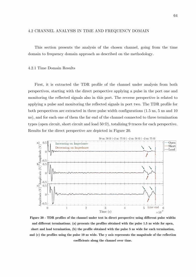
64
4.2 CHANNEL ANALYSIS IN TIME AND FREQUENCY DOMAIN
This section presents the analysis of the chosen channel, going from the time
domain to frequency domain approach as described on the methodology.
4.2.1 Time Domain Results
First, it is extracted the TDR profile of the channel under analysis from both
perspectives, starting with the direct perspective applying a pulse in the port one and
monitoring the reflected signals also in this port. The reverse perspective is related to
applying a pulse and monitoring the reflected signals in port two. The TDR profile for
both perspectives are extracted in three pulse width configurations (1.5 ns, 5 ns and 10
ns), and for each one of them the far end of the channel connected to three termination
types (open circuit, short circuit and load 50 ), totalizing 9 traces for each perspective.
Results for the direct perspective are depicted in Figure 20.
Figure 20 - TDR profiles of the channel under test in direct perspective using different pulse widths
and different terminations. (a) presents the profiles obtained with the pulse 1.5 ns wide for open,
short and load termination, (b) the profile obtained with the pulse 5 ns wide for each termination,
and (c) the profiles using the pulse 10 ns wide. The y axis represents the magnitude of the reflection
coefficients along the channel over time.

65
The end of the channel is given by the right time in the trace where the magnitude
of reflection for the short termination starts to assume different value in comparison to
the one using open circuit termination. For this case this event occurs at about 557 ns.
Considering the round trip of the incident/reflected signal, this channel is 278.5 ns
long.
On a first look at the profiles acquired for each pulse width set, it is clear a
similarity on shape and time between the traces. The initial variations read vary in
amplitude and dispersion. Knowing the channel and the disposition in which the
sections are through this perspective, there is no possibility to associate them with any
transition on the channel. The first transition for this perspective only occurs after
100 m (near at 500 ns) of round trip. Correlating the three profiles acquired, an initial
increasing on the reflection coefficient is observed at 13 ns. After that, a decreasing
followed by an increasing, but for these two there is no correlation in time between the
profiles. For each profile they differ by amplitude, time and dispersion. These evidences
may lead to correlate these initial variations to effects of the incident pulse over the
channel. Narrowing the pulse these effects are compressed in time and amplitude, as
can be verified.
The transitions between the sections can be verified at the far end of the channel
through this perspective. The reflection coefficient increases near at 497 ns, decreases
at 516 ns and increases back near at 537 ns, for the three cases.
It is evident the effect of resolution given by the pulse width difference. The
narrower the pulse, the higher the resolution obtained. The resolution for the 1.5 ns
trace for example is about 0.75 ns, which converted into space domain considering the
velocity of propagation of 66 % of the speed of light is equal to approximately 0.15 m.
For 5 ns wide, resolution will be 2.5 ns (0.495 m). For 10 ns wide, resolution is 5 ns
(0.99 m). Therefore, narrower pulses will lead to a more accurate analysis, as can be
verified in results through the shapes of changes on reflection coefficient at the end of
the channel for example. These shapes are more defined on the 1.5 ns traces, as their
changes are more abrupt in time. In other hand, narrowing the pulse comes with the
decreasing on its energy. The attenuation and distortion suffered by the pulse traveling
in round trip along the channel may lower its amplitude in a way which the reflections
cannot be identified at the reading end. In this case, the channel is short enough to
identify all the ones that matter, even for the narrowest pulse applied (1.5 ns).
However, for longer channels that would be a concern. This illustrates the trade-off on
choosing the pulse width and amplitude when applying reflectometry based methods.
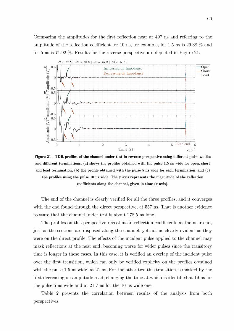
66
Comparing the amplitudes for the first reflection near at 497 ns and referring to the
amplitude of the reflection coefficient for 10 ns, for example, for 1.5 ns is 29.38 % and
for 5 ns is 71.92 %. Results for the reverse perspective are depicted in Figure 21.
Figure 21 - TDR profiles of the channel under test in reverse perspective using different pulse widths
and different terminations. (a) shows the profiles obtained with the pulse 1.5 ns wide for open, short
and load termination, (b) the profile obtained with the pulse 5 ns wide for each termination, and (c)
the profiles using the pulse 10 ns wide. The y axis represents the magnitude of the reflection
coefficients along the channel, given in time (x axis).
The end of the channel is clearly verified for all the three profiles, and it converges
with the end found through the direct perspective, at 557 ns. That is another evidence
to state that the channel under test is about 278.5 ns long.
The profiles on this perspective reveal mean reflection coefficients at the near end,
just as the sections are disposed along the channel, yet not as clearly evident as they
were on the direct profile. The effects of the incident pulse applied to the channel may
mask reflections at the near end, becoming worse for wider pulses since the transitory
time is longer in these cases. In this case, it is verified an overlap of the incident pulse
over the first transition, which can only be verified explicity on the profiles obtained
with the pulse 1.5 ns wide, at 21 ns. For the other two this transition is masked by the
first decreasing on amplitude read, changing the time at which is identified at 19 ns for
the pulse 5 ns wide and at 21.7 ns for the 10 ns wide one.
Table 2 presents the correlation between results of the analysis from both
perspectives.

67
Table 2 - Correlation between reflections of TDR profiles in both perspectives.
Perspective Direct Reverse
Section Duration Amplitude Duration Amplitude
1.5 ns 5 ns 10 ns 1.5 ns 5 ns 10 ns
50 W / 50.12
m
499.5 ns 0 0 0 497.5 ns 0 0 0
75 W / 1.97
m
19 ns 0.072 0.175 0.246 19.3 ns -0.207 -0.27 -0.31
50 W / 2.03
m
21.3 ns -0.031 -0.111 -0.17 20.5 ns 0.235 0.294 0.326
75 W / 2.07
m
20.1 ns 0.054 0.132 0.192 22.6 ns -0.230 -0.579 -0.829
It is verified a good agreement between the time for each section in both
perspectives, yet the difference verified for the maximum amplitude. The amplitude
difference is related to the distortion which the pulse suffers along the channel. The
pulse reflected at the near end of the channel will suffer a smaller attenuation than the
one reflected at the far end of the channel.
The analysis of the channel in time domain is also made by evaluating its impulse
response, thus composing the time domain transmissometry analysis. TDT is also
performed considering both perspectives of the channel. Results are shown in Figure
22.

68
Figure 22 - Impulse response of the channel under analysis. (a) depicts the response considering the
propagation through the direct perspective, while (b) for the contrary perspective.
The pulse takes about 272 ns to travel down the channel in both perspectives,
verified by the time in which the first pulse starts rising. It conflicts with the half time
for round trip achieved through the TDR analysis in both perspectives (278.5 ns),
resulting in a relative error of 2.33 %. The following pulses are related to second order
reflections, generated by reflections of the reflected signal over the transitions backward
propagating. Since the signal generator and the oscilloscope probe have an input
impedance of 50 , all the signals after the first pulse are generated by internals
reflections in the channel. This way what matters from this analysis is verifying how
long is the line and how distorted will be an incident pulse by the channel.
There is no clear difference verified comparing the impulse response acquired from
each perspective. Shape and amplitude over the time compound almost the same
response. The only differences noticed are related to the amplitudes comparing the
profiles obtained by different pulse widths for the same perspective. The attenuation
suffered by the channel is higher for narrower pulses, as already experimented in the
TDR profiles acquired. Taking the maximum amplitude acquired on the TDT profile
generated by the pulse 10 ns wide as 100 % (3.32 V), the 5 ns wide response has reached
82.53 %, and 40.96 % for the 1.5 ns wide one. The difference is notable and may be
related to the attenuation over the frequency components for each pulse width set.
Narrower pulses have more high frequency components than the wider ones, and since
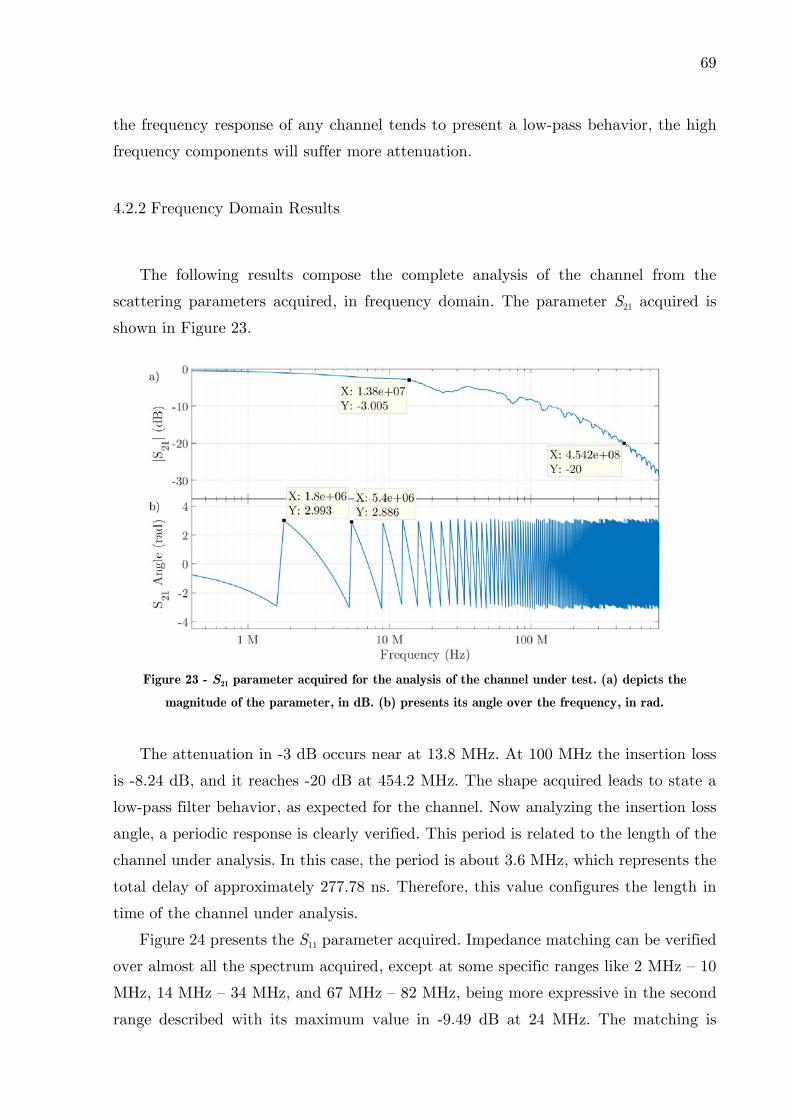
69
the frequency response of any channel tends to present a low-pass behavior, the high
frequency components will suffer more attenuation.
4.2.2 Frequency Domain Results
The following results compose the complete analysis of the channel from the
scattering parameters acquired, in frequency domain. The parameter S21 acquired is
shown in Figure 23.
Figure 23 - S21 parameter acquired for the analysis of the channel under test. (a) depicts the
magnitude of the parameter, in dB. (b) presents its angle over the frequency, in rad.
The attenuation in -3 dB occurs near at 13.8 MHz. At 100 MHz the insertion loss
is -8.24 dB, and it reaches -20 dB at 454.2 MHz. The shape acquired leads to state a
low-pass filter behavior, as expected for the channel. Now analyzing the insertion loss
angle, a periodic response is clearly verified. This period is related to the length of the
channel under analysis. In this case, the period is about 3.6 MHz, which represents the
total delay of approximately 277.78 ns. Therefore, this value configures the length in
time of the channel under analysis.
Figure 24 presents the S11 parameter acquired. Impedance matching can be verified
over almost all the spectrum acquired, except at some specific ranges like 2 MHz – 10
MHz, 14 MHz – 34 MHz, and 67 MHz – 82 MHz, being more expressive in the second
range described with its maximum value in -9.49 dB at 24 MHz. The matching is

70
related to the impedance of the measurement system, which is 50 in this case. At
the remaining spectrum the return loss parameter is under -20 dB.
Figure 24 – S11 parameter acquired for the analysis of the channel under test. (a) depicts the
magnitude of the parameter, in dB. (b) presents its angle over the frequency, in rad.
The analysis of the channel length is also possible through the periodic behavior of
the S11 angle, but now the round trip must be considered. The period verified is 1.8
MHz, which converted into time is about 555.56 ns. The channel length in time is half
this value, 277.78 ns, which is exactly the same time found by the analysis of the
periodic behavior of the S21 parameter.
Results of the conversion of the scattering parameters into time domain data are
presented in the two following figures, being the Figure 25 related to the parameters
S11 and S22 in time domain (reflection behavior) and Figure 26 to the parameters S21
and S12 in time domain (transmission behavior). Both figures present results of the
conversion performed by ICZT and Sparse ICZT in comparison to time domain profiles
acquired using the 1.5 ns wide pulse. The choice of the pulse width profiles was made
considering their higher resolution in comparison to the other ones acquired. A scaling
factor of 0.143 in amplitude was applied to the TDR signals to enable a better viewing
scenario for the comparison with ICZT and Sparse ICZT results. It is important to
remember that the TDR signals are purely voltage signals created by the reflection of
the incident pulse, whereas ICZT and Sparse ICZT are normalized coefficients
generated by the conversions.

71
Figure 25 – Analysis of the parameters S11 and S22 in time domain, given by the conversion performed
by ICZT and Sparse ICZT, in comparison to the TDR profile acquired. (a) is related to the direct
perspective of the channel, whereas (b) to the reverse perspective.
Analyzing the conversion of the parameter S11 in time domain, it is possible to
verify four transitions along the channel, all of them concentrated at the far end of the
channel. The first transition happens near at 496 ns, corresponding to an increasing on
the characteristic impedance. Then, after 20 ns a second transition designated by a
decreasing on it. Following the signal, after 20 ns there is an increasing on the
characteristic impedance representing the third transition. The last transition, near at
557 ns, represents a decreasing one. Correlating these results with the channel under
analysis, the transitions are verified just as the sections are disposed in time / length
along the channel through this perspective, as well the change tendencies on the
characteristic impedance. The last transition corresponds to the end of the channel,
which is the border between the section with characteristic impedance in 75 and the
network analyzer input impedance of 50 . That is why its magnitude is similar to the
one related to the transition from second to third section (75 to 50 ).
Now analyzing the parameter S22 in time domain, three transitions are clear to
identify at the near end: a decreasing near at 21 ns, an increasing near at 41 ns, and a
last decreasing near at 61 ns. The transitions are disposed just as the sections are in
the channel through the reverse perspective. In this case, the magnitudes are higher
than the ones obtained from the other perspective. The network analyzer equipment

72
acquires the parameters at one frequency at a time. Since the channel behaves as a low
pass filter, each frequency component of the interrogator signal will suffer a different
attenuation. Moreover, there is also the attenuation over the channel length. That is
why the same section transitions have presented different amplitudes comparing the
scattering parameters acquired for each perspective converted to time domain.
For both perspective profiles given by the conversion of the scattering parameters
S11 and S22 it is verified a good agreement in shape and time between results obtained
by ICZT and Sparse ICZT. The most explicit difference is related to the amplitude,
with an average difference in about 77.04 %, Sparse ICZT referred to ICZT.
Table 3 presents a comparison between the transition times in profiles obtained
with the conventional ICZT and the Sparse ICZT method, as well the correlation
between the duration for each section through each perspective. It is also presented
information about the TDR profiles acquired, in a way to compare them with their
respective scattering parameters converted into time domain.
Table 3 - Correlation between the scattering parameters S11 and S22 in time domain, obtained by
ICZT and Sparse ICZT, and TDR profiles.
Perspective Direct (S11) Reverse (S22)
Section ICZT Sparse
ICZT
TDR
1.5 ns
ICZT Sparse
ICZT
TDR
1.5 ns
50 W / 50.12
m
Transition at
Length
496.6 ns
496.6 ns
496.6 ns
496.6 ns
499.5 ns
499.5 ns
556.6 ns
496 ns
556.6 ns
496 ns
559.9 ns
497.5 ns
75 W / 1.97
m
Transition at
Length
516.6 ns
20 ns
516 ns
19.4 ns
518.5 ns
19 ns
60.6 ns
19.4 ns
60.6 ns
19.4 ns
62.4 ns
19.3 ns
50 W / 2.03
m
Transition at
Length
537.2 ns
20.6 ns
536.5 ns
20.5 ns
539.8 ns
21.3 ns
41.2 ns
20.6 ns
41.2 ns
20.6 ns
43.1 ns
20.5 ns
75 W / 2.07
m
Transition at
Length
557.8 ns
20.6 ns
556.6 ns
20.1 ns
559.9 ns
20.1 ns
20.6 ns
20.6 ns
20.6 ns
20.6 ns
22.6 ns
22.6 ns
Correlating the sections identified through each perspective, the maximum
difference for time duration of each one is about 0.6 ns for ICZT and Sparse ICZT
conversions, and 2.5 ns for TDR profiles, which correspond in length to 3 cm and 12.4
cm respectively. These errors represent 0.05 % and 0.022 % of total the length of the
channel under analysis, revealing the good correlation between the scattering
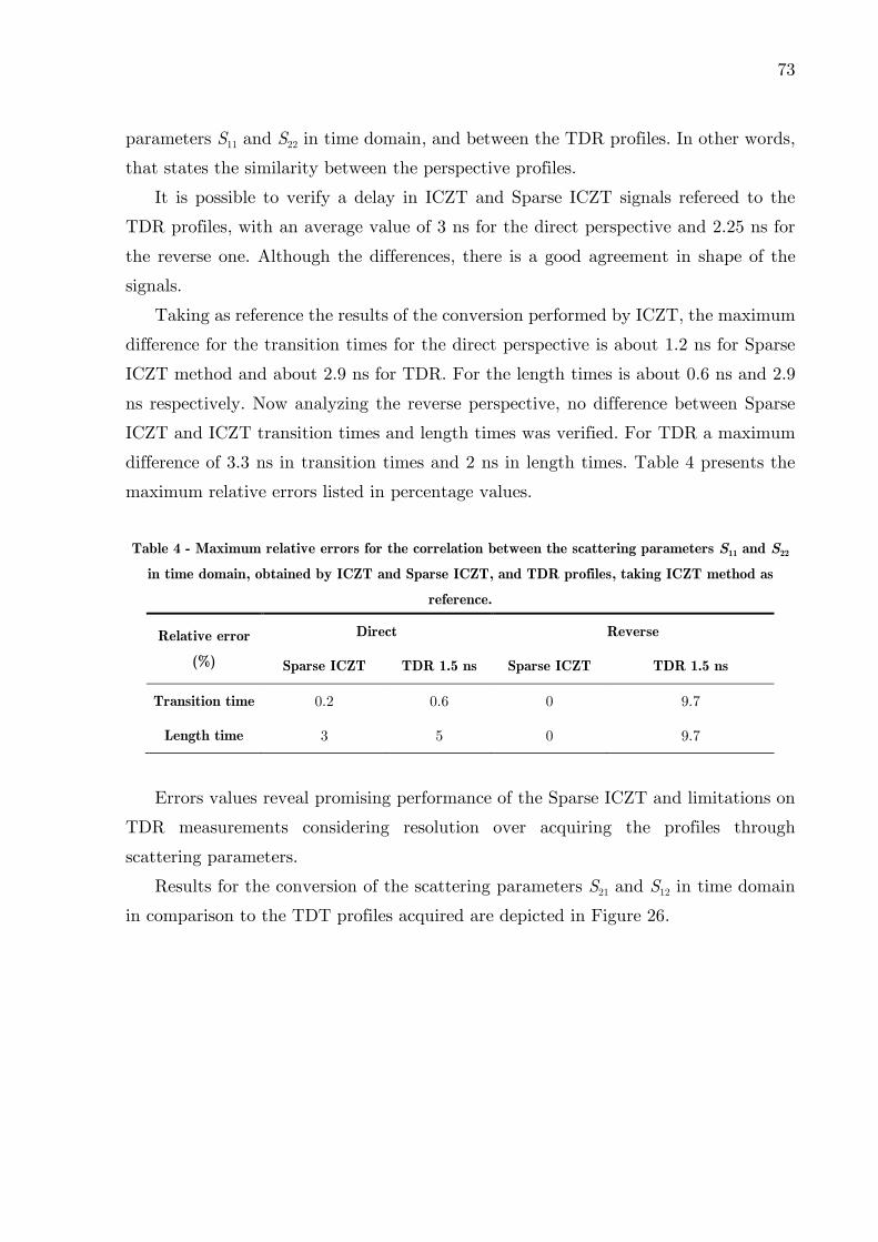
73
parameters S11 and S22 in time domain, and between the TDR profiles. In other words,
that states the similarity between the perspective profiles.
It is possible to verify a delay in ICZT and Sparse ICZT signals refereed to the
TDR profiles, with an average value of 3 ns for the direct perspective and 2.25 ns for
the reverse one. Although the differences, there is a good agreement in shape of the
signals.
Taking as reference the results of the conversion performed by ICZT, the maximum
difference for the transition times for the direct perspective is about 1.2 ns for Sparse
ICZT method and about 2.9 ns for TDR. For the length times is about 0.6 ns and 2.9
ns respectively. Now analyzing the reverse perspective, no difference between Sparse
ICZT and ICZT transition times and length times was verified. For TDR a maximum
difference of 3.3 ns in transition times and 2 ns in length times. Table 4 presents the
maximum relative errors listed in percentage values.
Table 4 - Maximum relative errors for the correlation between the scattering parameters S11 and S22
in time domain, obtained by ICZT and Sparse ICZT, and TDR profiles, taking ICZT method as
reference.
Relative error
(%)
Direct Reverse
Sparse ICZT TDR 1.5 ns Sparse ICZT TDR 1.5 ns
Transition time 0.2 0.6 0 9.7
Length time 3 5 0 9.7
Errors values reveal promising performance of the Sparse ICZT and limitations on
TDR measurements considering resolution over acquiring the profiles through
scattering parameters.
Results for the conversion of the scattering parameters S21 and S12 in time domain
in comparison to the TDT profiles acquired are depicted in Figure 26.

74
Figure 26 - Analysis of the parameters S21 and S12 in time domain, presenting results of the conversion
performed by ICZT and Sparse ICZT, in comparison to the TDT profile acquired. (a) presents the
parameter S21 in time domain, related to the direct perspective propagation. (b) presents the
parameter S12 in time domain, related to the reverse perspective propagation.
These parameters in time domain are related to the impulse response of the channel
under analysis, revealing the delay and attenuation caused by the channel. On a first
look, it is verified the similarity in behavior between them. That means that there will
be no difference propagating a signal through this channel in any perspective. The
delay is about 278.6 ns for both parameters S21 and S12 in time domain for both
conversion methods, whereas for the TDT profiles is about 274.5 ns for both
perspectives. Although, the amplitudes obtained also diverges from one to the other.
The amplitude in both perspectives of the first pulse is 0.157 for ICZT, while for Sparse
ICZT is 0.105. For a better comparison, a scaling factor of 0.143 in amplitude was
applied to the TDT signals, remembering that they are purely voltage signals, whereas
ICZT and Sparse ICZT are normalized coefficients.
Back to the analysis of the scattering parameters in the frequency domain, first it
is extracted the secondary parameters characteristic impedance and propagation
constant. In Figure 27 the results for the characteristic impedance are depicted, in
absolute values. The characteristic impedance also presents a periodic behavior that
reveals the length of the channel under test, with period in 1.8 MHz. It varies in
magnitude from 30 to 80 for frequencies lower than 33.8 MHz. After that it keeps
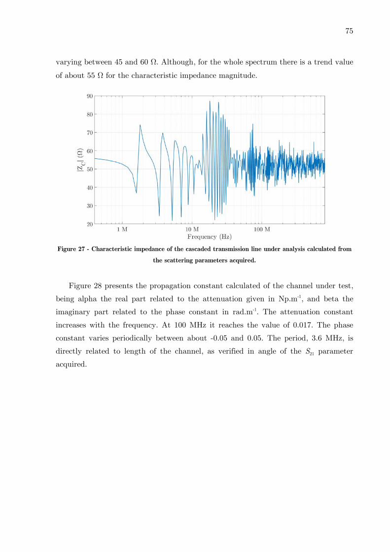
75
varying between 45 and 60 . Although, for the whole spectrum there is a trend value
of about 55 for the characteristic impedance magnitude.
Figure 27 - Characteristic impedance of the cascaded transmission line under analysis calculated from
the scattering parameters acquired.
Figure 28 presents the propagation constant calculated of the channel under test,
being alpha the real part related to the attenuation given in Np.m-1, and beta the
imaginary part related to the phase constant in rad.m-1. The attenuation constant
increases with the frequency. At 100 MHz it reaches the value of 0.017. The phase
constant varies periodically between about -0.05 and 0.05. The period, 3.6 MHz, is
directly related to length of the channel, as verified in angle of the S21 parameter
acquired.
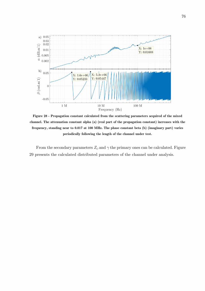
76
Figure 28 - Propagation constant calculated from the scattering parameters acquired of the mixed
channel. The attenuation constant alpha (a) (real part of the propagation constant) increases with the
frequency, standing near to 0.017 at 100 MHz. The phase constant beta (b) (imaginary part) varies
periodically following the length of the channel under test.
From the secondary parameters ZC and the primary ones can be calculated. Figure
29 presents the calculated distributed parameters of the channel under analysis.
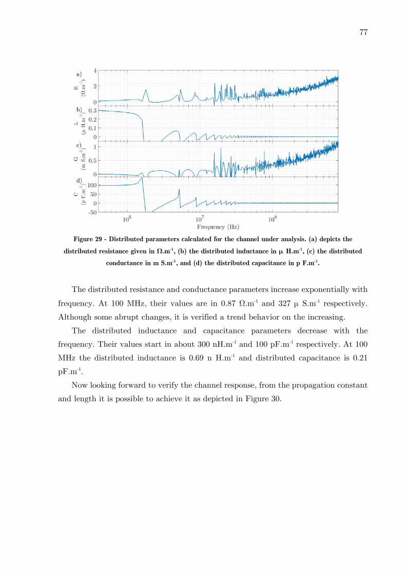
77
Figure 29 - Distributed parameters calculated for the channel under analysis. (a) depicts the
distributed resistance given in W.m-1, (b) the distributed inductance in µ H.m-1, (c) the distributed
conductance in m S.m-1, and (d) the distributed capacitance in p F.m-1.
The distributed resistance and conductance parameters increase exponentially with
frequency. At 100 MHz, their values are in 0.87 .m-1 and 327 µ S.m-1 respectively.
Although some abrupt changes, it is verified a trend behavior on the increasing.
The distributed inductance and capacitance parameters decrease with the
frequency. Their values start in about 300 nH.m-1 and 100 pF.m-1 respectively. At 100
MHz the distributed inductance is 0.69 n H.m-1 and distributed capacitance is 0.21
pF.m-1.
Now looking forward to verify the channel response, from the propagation constant
and length it is possible to achieve it as depicted in Figure 30.
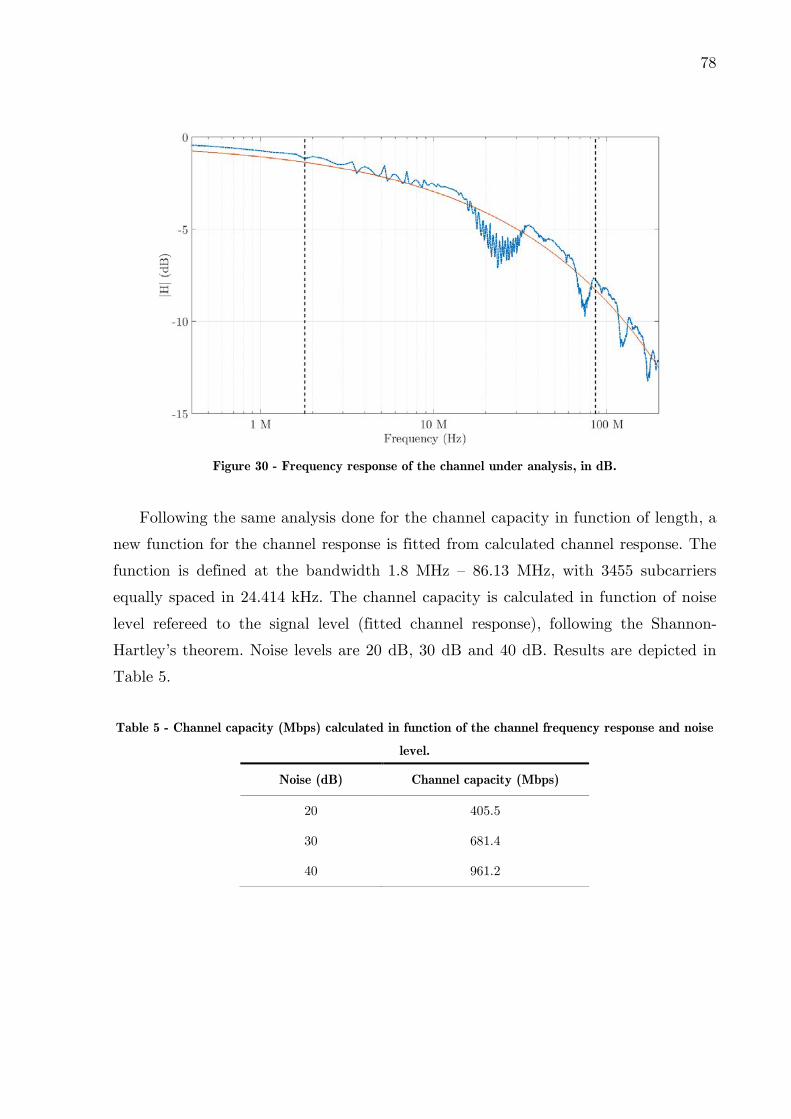
78
Figure 30 - Frequency response of the channel under analysis, in dB.
Following the same analysis done for the channel capacity in function of length, a
new function for the channel response is fitted from calculated channel response. The
function is defined at the bandwidth 1.8 MHz – 86.13 MHz, with 3455 subcarriers
equally spaced in 24.414 kHz. The channel capacity is calculated in function of noise
level refereed to the signal level (fitted channel response), following the Shannon-
Hartley’s theorem. Noise levels are 20 dB, 30 dB and 40 dB. Results are depicted in
Table 5.
Table 5 - Channel capacity (Mbps) calculated in function of the channel frequency response and noise
level.
Noise (dB) Channel capacity (Mbps)
20 405.5
30 681.4
40 961.2
79
5 CONCLUSIONS
Electrical cable networks are widely employed for energy distribution and
communication systems. In many applications, such cables are exposed to harsh
environments. Subsea systems in the oil industry are a typical example. The demand
for maximum power transfer, less susceptible to electromagnetic interference and
greater transmission rates requires the analysis of the transmission lines parameters in
details and continuously.
In this work a study of techniques for analysis of transmission lines in time and
frequency domain is presented. To evaluate the influence of length on the channel
capacity, the capacity was obtained from scattering parameters of an unshielded
twisted pair CAT5e in ten different lengths. Here the assumption that the signal level
is limited by the bandwidth of 1.8 MHz to 86 MHz was taken, following the HomePlug
AV2 specifications, which was taken as commercial example of communication system
for the sake performance evaluation. Results are curves of the channel capacity for
different noise levels in function of length. From them it is possible to evaluate the
maximum rates for each length in different SNR conditions. The same experiment was
done using a two wire stranded copper 1.5 mm² cable. Due to its constructive
characteristics the scattering parameters acquired has presented an unstable behavior
in comparison to the other cable. Although, for both kinds it is verified the relationship
between the length and maximum capacity. For both cables it was verified a
performance beyond the 20 dB noise level capacity curve and below the 30 dB curve,
suggesting the PLC working noise level.
Looking forward to understand techniques for the analysis of transmission lines in
time and frequency domain, a set of analysis for a chosen transmission line
configuration is also proposed, composed by four sections of coaxial cables with different
lengths and characteristic impedance alternating between 50 and 75 . The analysis
started in time domain with the extraction of TDR and TDT profiles of the channel,
for both perspectives of reflection and transmission respectively, and in three different
pulse width configurations. Through the results it was observed the effects of trade-off
between pulse width and amplitude over the profile resolution. The narrower the pulse
the greater the resolution, even though the energy decreasing by it also implies a
decreasing on the energy of the reflected pulse and might cause its vanish. The analysis

80
of the profiles acquired allows the verification of type and location of impedance
transitions along the line, as well its length and impulse response.
The analysis of the channel under test in frequency domain starts with the
extraction of the scattering parameters. From them it is calculated the secondary
parameters of the line characteristic impedance and propagation constant. These
parameters reveal the behavior of the channel over the frequency spectrum acquired,
and knowing its length lead to the primary ones: distributed resistance, inductance,
conductance and capacitance.
From scattering parameters it is also possible the analysis of the channel in time
domain, given by the Inverse Chirp Z Transform. In this work, a sparse approach for
this inverse problem is also proposed, since the nature of the impedance mismatches
along a transmission line is sparse. Results of the conversion solved by the proposed
method are compared to the ones obtained by the conventional Inverse Chirp Z
Transform. Through the comparison, it is verified a good agreement in time location
and wave shape of the signals, revealing promising results in time domain analysis of
scattering parameters.
5.1 FUTURE WORK
The presented work opens horizons to the development of more complex and
detailed studies on techniques for characterizing channels field. It is suggested the
application of the proposed sets of experiment using a real network managed by a real
communication system, in a way to achieve the maximum capacity at the environment
in which the system runs. This will require the study in details of proper noise models
and of the technology used by the system modems.
Moreover, on the channel characterization in time and frequency domain, it is
suggested an investigation and application of more complex methods for obtaining the
impedance profile of the line, so that the reflections coefficients can be achieved purely,
with no influence of second order reflections. In addition, the performance of the
proposed method Sparse Inverse Chirp Z Transform for time domain analysis of
transmission lines must be evaluated, being suggested to be compared to the
conventional Inverse Chirp Z Transform method.
81
REFERENCES
AGILENT TECHNOLOGIES. S-Parameter Design - Application note 154, 2006.
AGILENT TECHNOLOGIES. Time Domain Analysis Using a Network Analyzer -
Application note 1287-12, 2012.
AGILENT TECHNOLOGIES. Time Domain Reflectometry Theory - Application note
1304-2, 2013.
ALLIANCE, P.; RESERVED, A. R. HomePlug AV White Paper. Architecture, p. 1–
11, 2005.
ALLIANCE HPGP. HomePlug TM AV2 technology. HomePlug Powerline Alliance, Inc,
p. 1–12, 2013.
ANRISTU. A Guide to Making RF Measurements for Signal Integrity Applications,
2016.
BAHAI, A. R. S.; SALTZBERG, B. R.; ERGEN, M. Multi-Carrier Digital
Communications: Theory and Applications of OFDM. Second ed. Springer, 2004.
BECK, A.; TEBOULLE, M. Fast Gradient-Based Algorithms for Constrained Total
Variation Image Denoising and Deblurring Problems. IEEE Transactions on Image
Processing, v. 18, n. 11, p. 2419–2434, 2009a.
BECK, A.; TEBOULLE, M. A Fast Iterative Shrinkage-Thresholding Algorithm.
Society for Industrial and Applied Mathematics Journal on Imaging Sciences, v. 2, n.
1, p. 183–202, 2009b.
82
BEGOVIC, A.; SKALJO, N.; GORAN, N. An example of estimation of twisted pair
channel capacity in DSL environment. 1st International Conference on
Communications, Signal Processing, and their Applications (ICCSPA). IEEE, feb. 2013
BLEMEL, K.; FURSE, C. Applications of microsystems and signal processing for
wiring integrity monitoring. 2001 IEEE Aerospace Conference Proceedings (Cat.
No.01TH8542). IEEE, 2001
CHING-WEN HSUE; TE-WEN PAN. Reconstruction of nonuniform transmission lines
from time-domain reflectometry. IEEE Transactions on Microwave Theory and
Techniques, v. 45, n. 1, p. 32–38, 1997.
DE PORRATA-DORIA I YAGUE, R.; IBARS, A. B.; MARTINEZ, L. F. Analysis
and reduction of the distortions induced by time-domain filtering techniques in network
analyzers. IEEE Transactions on Instrumentation and Measurement, v. 47, n. 4, p.
930–934, 1998.
DRAKA. UC300 24 Cat.5e DatasheetDraka Prysmian Group, , 2017. Available on:
<https://www.prysmiangroup.com/sites/default/files/business_markets/markets/do
wnloads/datasheets/da13e_0.pdf>
DUNSMORE, J.; CHENG, N.; ZHANG, Y. Characterizations of asymmetric fixtures
with a two-gate approach. 77th ARFTG Microwave Measurement Conference. IEEE,
jun. 2011
EZZINE, S. et al. Evaluation of PLC channel capacity and ABER performances for
OFDM-based two-hop relaying transmission. Wireless Communications and Mobile
Computing, 2017.
FRANCIS, A.; TITUS, G. Channel capacity analysis of railway power lines. 2011
International Conference on Emerging Trends in Electrical and Computer Technology.

83
IEEE, mar. 2011
FRICKEY, D. A. Using the Inverse Chirp-Z Transform for Time-Domain Analysis of
Simulated Radar Signals. ICSPAT 94: signal procession applications and technology,
p. 1–6, 1994.
GOLDSMITH, A. Wireless Communications. Cambridge: Cambridge University Press,
2005.
HAYT, W. H.; BUCK, J. A. Engineering Electromagnetics. Engineering
Electromagnetics, p. 563, 2011.
HERNANDEZ-MEJIA, J. C. Time Domain Reflectometry. Neetrac Georgia Tech,
2016.
IDA, N. Engineering Electromagnetics. Third ed. Cham: Springer International
Publishing, 2015.
KOTCHASARN, C. Performance Analysis of Broadband Power Line Communications
with OFDM Transmission. p. 316–320, 2017.
KWAK, K. S. et al. Reduction of the blind spot in the time-frequency domain
reflectometry. IEICE Electronics Express, v. 5, n. 8, p. 265–270, 2008.
LAMPE, L.; TONELLO, A. M.; SWART, T. G. Power Line Communications:
Principles, Standards and Applications from Multimedia to Smart Grid. Second ed.
Chichester, UK: John Wiley & Sons, Ltd, 2016.
LIN, Y.-P.; PHOONG, S.-M.; VAIDYANATHAN, P. P. Filter bank transceivers for
OFDM and DMT systems. First ed. Cambridge: Cambridge University Press, 2011.

84
MERSEREAU, R. An Algorithm for Performing an Inverse Chirp Z-Transform. IEEE
Transactions on Acoustics, Speech, and Signal Processing, v. 22, n. 5, p. 387–388, oct.
1974.
PAPAZYAN, R. et al. Extraction of high frequency power cable characteristics from
S-parameter measurements. IEEE Transactions on Dielectrics and Electrical
Insulation, v. 11, n. 3, p. 261–270, jun. 2004.
PASTERNACK. Flexible RG58 Coax Cable Single Shielded with Black PVC Jacket
DatasheetPasternack Enterprises, , 2017. Available on:
<https://www.pasternack.com/images/ProductPDF/RG58C-U.pdf>
POZAR, D. Microwave Engineering. Fourth ed. John Wiley & Sons, Inc., 2005.
QINGHAI SHI; KANOUN, O. Wire Fault Diagnosis in the Frequency Domain by
Impedance Spectroscopy. IEEE Transactions on Instrumentation and Measurement, v.
64, n. 8, p. 2179–2187, aug. 2015.
QINGHAI SHI; TROLTZSCH, U.; KANOUN, O. Analysis of the parameters of a lossy
coaxial cable for cable fault location. Eighth International Multi-Conference on
Systems, Signals & Devices. IEEE, mar. 2011
RABINER, L.; SCHAFER, R.; RADER, C. The Chirp Z-Transform Algorithm. IEEE
Transactions on Audio and Electroacoustics, v. 17, n. 2, p. 86–92, jun. 1969.
RAHMAN, M. M.; MAJUMDER, S. P. Performance analysis of a OFDM SISO
powerline communication system with non-white Gaussian channel noise. 1st
International Conference on Electrical Engineering and Information and
Communication Technology, ICEEICT 2014, p. 1–4, 2014.

85
RITO, M.-C. et al. Communications System for Down-Hole Measurements. Journal of
Applied Research and Technology, v. 11, n. 6, p. 903–911, dec. 2013.
ROHLING, H. OFDM. Concepts for Future Communication Systems. Berlin,
Heidelberg: Springer Berlin Heidelberg, 2011.
SHANNON, C. E. A Mathematical Theory of Communication. Bell System Technical
Journal, v. 27, n. 3, p. 379–423, 1 jul. 1948.
SHANNON, C. E. Communication in the Presence of Noise. Proceedings of the IRE,
v. 37, n. 1, p. 10–21, jan. 1949.
SHI, Q.; KANOUN, O. Wire fault location in coaxial cables by impedance spectroscopy.
IEEE Sensors Journal, v. 13, n. 11, p. 4465–4473, 2013.
SMITH, P.; FURSE, C.; GUNTHER, J. Analysis of spread spectrum time domain
reflectometry for wire fault location. IEEE Sensors Journal, v. 5, n. 6, p. 1469–1478,
dec. 2005.
VAN HAMME, H. High-resolution frequency-domain reflectometry by estimation of
modulated superimposed complex sinusoids. IEEE Transactions on Instrumentation
and Measurement, v. 41, n. 6, p. 762–767, 1992.
VANHAMME, H. High resolution frequency-domain reflectometry. IEEE Transactions
on Instrumentation and Measurement, v. 39, n. 2, p. 369–375, apr. 1990.
VEIJOLA, T. V.; VALTONEN, M. E. Identification of cascaded microwave circuits
with moderate reflections using reflection and transmission measurements. IEEE
Transactions on Microwave Theory and Techniques, v. 36, n. 2, p. 418–423, 1988.
86
WALSH, J. F. Dual Time Base Zero Dead Zone Time Domain Reflectometer. United
States Patent, 1995.
WEBER, G. H. et al. Sparse Inverse Chirp-Z Transform of S-Parameter
Measurements for Time Domain Analysis of Transmission Line. XXXV Simpósio
Brasileiro de Telecomunicações e Processamento de Sinais - SBrT2017. São Pedro: 2017
YAMADA, T.; HIRAI, N.; OHKI, Y. Improvement in sensitivity of broadband
impedance spectroscopy for locating degradation in cable insulation by ascending the
measurement frequency. 2012 IEEE International Conference on Condition Monitoring
and Diagnosis. IEEE, sep. 2012
YONGE, L. et al. An Overview of the HomePlug AV2 Technology. Journal of Electrical
and Computer Engineering, v. 2013, p. 1–20, 2013.
ZYARI, M.; ROLAIN, Y. Identifying Multiple Reflections in Distributed-Lumped
High-Frequency Structures. IEEE Transactions on Microwave Theory and Techniques,
v. 64, n. 4, p. 1306–1312, apr. 2016.


