

Classification: Basic Concepts, Decision Trees, and Model Evaluation
Lecture Notes for Chapter 4
Introduction to Data MiningBy Tan, Steinbach, Kumar
1 1
Edited by Dr. Panagiotis Symeonidis Data Engineering Laboratory
http://delab.csd.auth.gr/~symeonhttp://delab.csd.auth.gr/~symeon
Classification: Definition
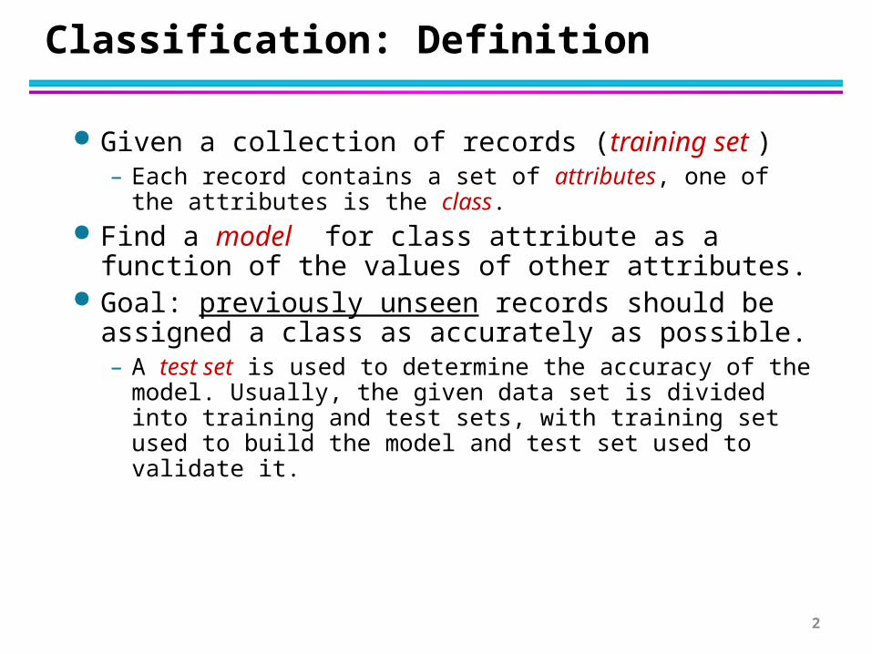
Given a collection of records (training set )– Each record contains a set of attributes, one of the
attributes is the class. Find a model for class attribute as a function
of the values of other attributes. Goal: previously unseen records should be
assigned a class as accurately as possible.– A test set is used to determine the accuracy of the
model. Usually, the given data set is divided into training and test sets, with training set used to build the model and test set used to validate it.
2

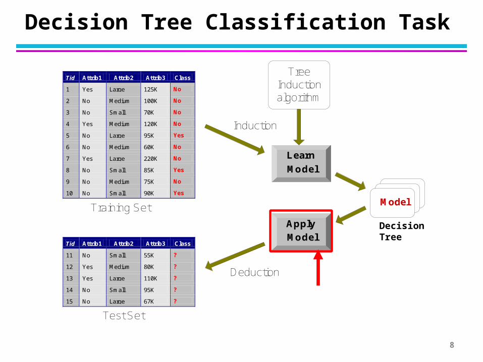
Illustrating Classification Task
Apply
Model
Induction
Deduction
Learn
Model
Model
Tid Attrib1 Attrib2 Attrib3 Class
1 Yes Large 125K No
2 No Medium 100K No
3 No Small 70K No
4 Yes Medium 120K No
5 No Large 95K Yes
6 No Medium 60K No
7 Yes Large 220K No
8 No Small 85K Yes
9 No Medium 75K No
10 No Small 90K Yes 10
Tid Attrib1 Attrib2 Attrib3 Class
11 No Small 55K ?
12 Yes Medium 80K ?
13 Yes Large 110K ?
14 No Small 95K ?
15 No Large 67K ? 10
Test Set
Learningalgorithm
Training Set
3
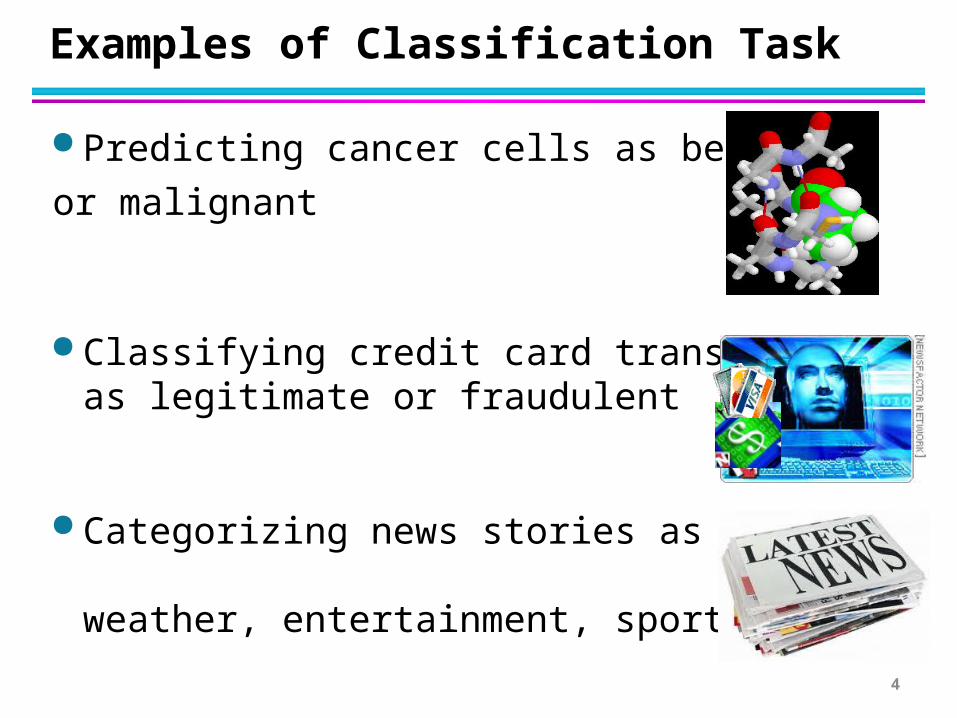
Examples of Classification Task
Predicting cancer cells as benign
or malignant
Classifying credit card transactions as legitimate or fraudulent
Categorizing news stories as finance, weather, entertainment, sports, etc
4
Classification Techniques
Decision Tree based Methods Association Rule based Methods Memory based Methods (e.g. k Nearest
Neighbor) Naïve Bayes Classifier Ensemble Methods (Bagging or Boosting)
5
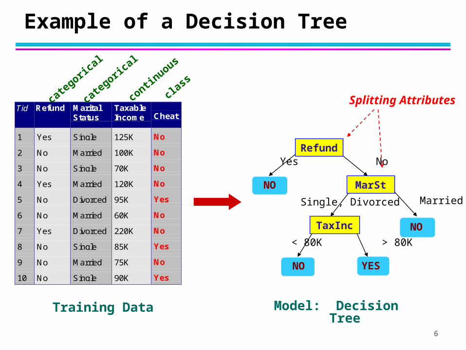
Example of a Decision Tree
Tid Refund MaritalStatus
TaxableIncome Cheat
1 Yes Single 125K No
2 No Married 100K No
3 No Single 70K No
4 Yes Married 120K No
5 No Divorced 95K Yes
6 No Married 60K No
7 Yes Divorced 220K No
8 No Single 85K Yes
9 No Married 75K No
10 No Single 90K Yes10
categoric
al
categoric
al
continuous
class
Refund
MarSt
TaxInc
YESNO
NO
NO
Yes No
Married Single, Divorced
< 80K > 80K
Splitting Attributes
Training Data Model: Decision Tree
6

Another Example of Decision Tree
Tid Refund MaritalStatus
TaxableIncome Cheat
1 Yes Single 125K No
2 No Married 100K No
3 No Single 70K No
4 Yes Married 120K No
5 No Divorced 95K Yes
6 No Married 60K No
7 Yes Divorced 220K No
8 No Single 85K Yes
9 No Married 75K No
10 No Single 90K Yes10
categoric
al
categoric
al
continuous
classMarSt
Refund
TaxInc
YESNO
NO
NO
Yes No
Married Single,
Divorced
< 80K > 80K
There could be more than one tree that fits the same data!
7
Decision Tree Classification Task
Apply
Model
Induction
Deduction
Learn
Model
Model
Tid Attrib1 Attrib2 Attrib3 Class
1 Yes Large 125K No
2 No Medium 100K No
3 No Small 70K No
4 Yes Medium 120K No
5 No Large 95K Yes
6 No Medium 60K No
7 Yes Large 220K No
8 No Small 85K Yes
9 No Medium 75K No
10 No Small 90K Yes 10
Tid Attrib1 Attrib2 Attrib3 Class
11 No Small 55K ?
12 Yes Medium 80K ?
13 Yes Large 110K ?
14 No Small 95K ?
15 No Large 67K ? 10
Test Set
TreeInductionalgorithm
Training Set
Decision Tree
8

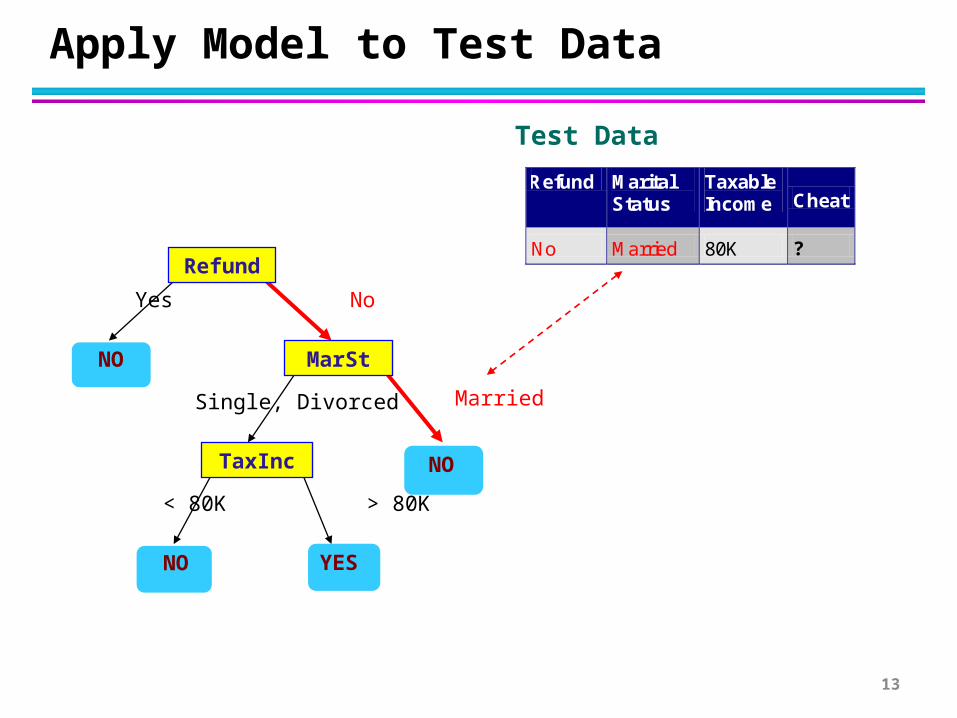
Apply Model to Test Data
Refund
MarSt
TaxInc
YESNO
NO
NO
Yes No
Married Single, Divorced
< 80K > 80K
Refund Marital Status
Taxable Income Cheat
No Married 80K ? 10
Test DataStart from the root of tree.
9

Apply Model to Test Data
Refund
MarSt
TaxInc
YESNO
NO
NO
Yes No
Married Single, Divorced
< 80K > 80K
Refund Marital Status
Taxable Income Cheat
No Married 80K ? 10
Test Data
10

Apply Model to Test Data
Refund
MarSt
TaxInc
YESNO
NO
NO
Yes No
Married Single, Divorced
< 80K > 80K
Refund Marital Status
Taxable Income Cheat
No Married 80K ? 10
Test Data
11

Apply Model to Test Data
Refund
MarSt
TaxInc
YESNO
NO
NO
Yes No
Married Single, Divorced
< 80K > 80K
Refund Marital Status
Taxable Income Cheat
No Married 80K ? 10
Test Data
12
Apply Model to Test Data
Refund
MarSt
TaxInc
YESNO
NO
NO
Yes No
Married Single, Divorced
< 80K > 80K
Refund Marital Status
Taxable Income Cheat
No Married 80K ? 10
Test Data
13
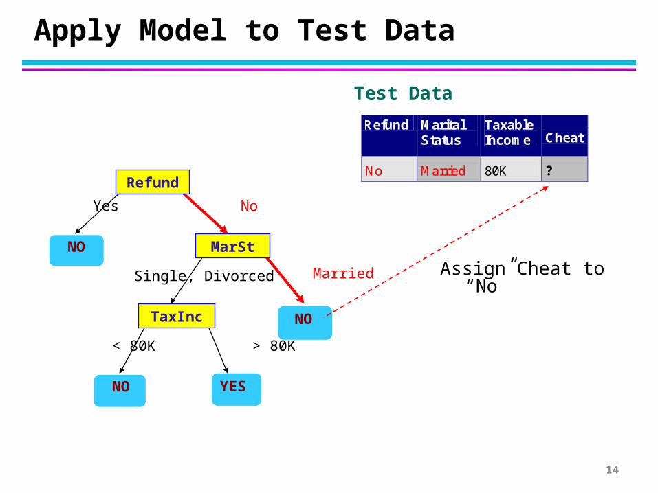
Apply Model to Test Data
Refund
MarSt
TaxInc
YESNO
NO
NO
Yes No
Married Single, Divorced
< 80K > 80K
Refund Marital Status
Taxable Income Cheat
No Married 80K ? 10
Test Data
Assign Cheat to “No”
14
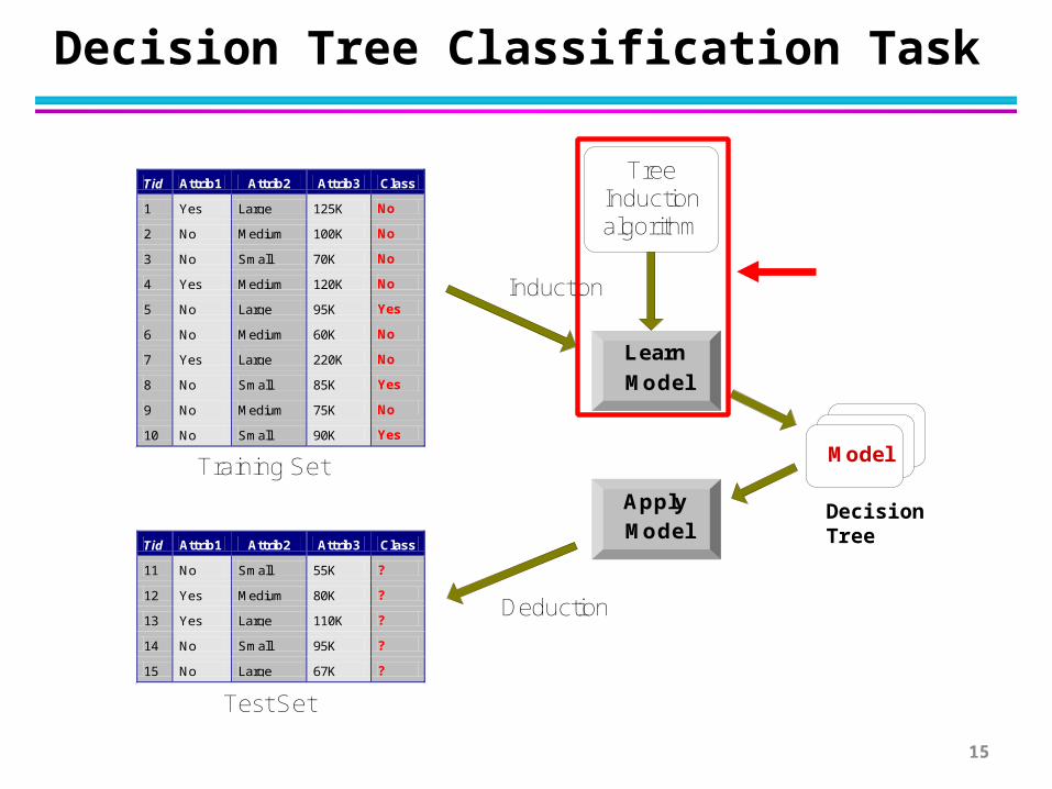
Decision Tree Classification Task
Apply
Model
Induction
Deduction
Learn
Model
Model
Tid Attrib1 Attrib2 Attrib3 Class
1 Yes Large 125K No
2 No Medium 100K No
3 No Small 70K No
4 Yes Medium 120K No
5 No Large 95K Yes
6 No Medium 60K No
7 Yes Large 220K No
8 No Small 85K Yes
9 No Medium 75K No
10 No Small 90K Yes 10
Tid Attrib1 Attrib2 Attrib3 Class
11 No Small 55K ?
12 Yes Medium 80K ?
13 Yes Large 110K ?
14 No Small 95K ?
15 No Large 67K ? 10
Test Set
TreeInductionalgorithm
Training Set
Decision Tree
15
Decision Tree Induction
Many Algorithms:
– Hunt’s Algorithm (one of the earliest)
– CART
– ID3, C4.5
– SLIQ,SPRINT
16
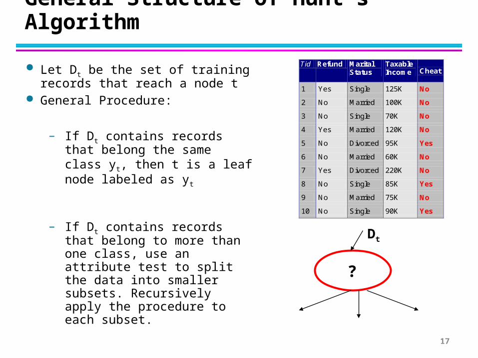
General Structure of Hunt’s Algorithm
Let Dt be the set of training records that reach a node t
General Procedure:
– If Dt contains records that belong the same class yt, then t is a leaf node labeled as yt
– If Dt contains records that belong to more than one class, use an attribute test to split the data into smaller subsets. Recursively apply the procedure to each subset.
Tid Refund Marital Status
Taxable Income Cheat
1 Yes Single 125K No
2 No Married 100K No
3 No Single 70K No
4 Yes Married 120K No
5 No Divorced 95K Yes
6 No Married 60K No
7 Yes Divorced 220K No
8 No Single 85K Yes
9 No Married 75K No
10 No Single 90K Yes 10
Dt
?
17
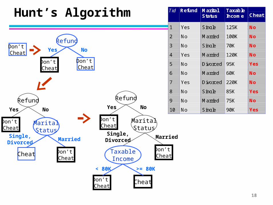
Hunt’s Algorithm
Don’t Cheat
Refund
Don’t Cheat
Don’t Cheat
Yes No
Refund
Don’t Cheat
Yes No
MaritalStatus
Don’t Cheat
Cheat
Single,Divorced
Married
TaxableIncome
Don’t Cheat
< 80K >= 80K
Refund
Don’t Cheat
Yes No
MaritalStatus
Don’t Cheat
Cheat
Single,Divorced
Married
18
Tree Induction
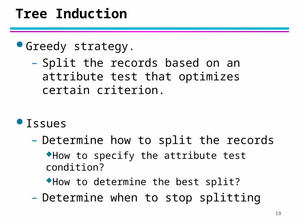
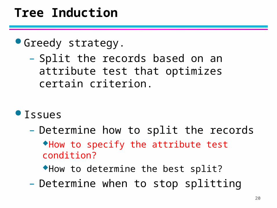
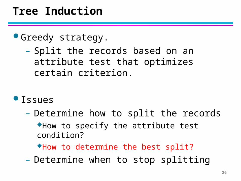
Greedy strategy.
– Split the records based on an attribute test that optimizes certain criterion.
Issues
– Determine how to split the recordsHow to specify the attribute test condition?How to determine the best split?
– Determine when to stop splitting
19
Tree Induction
Greedy strategy.
– Split the records based on an attribute test that optimizes certain criterion.
Issues
– Determine how to split the recordsHow to specify the attribute test condition?How to determine the best split?
– Determine when to stop splitting
20
How to Specify Test Condition?
Depends on attribute types
– Nominal
– Ordinal
– Continuous
Depends on number of ways to split
– 2-way split
– Multi-way split
21
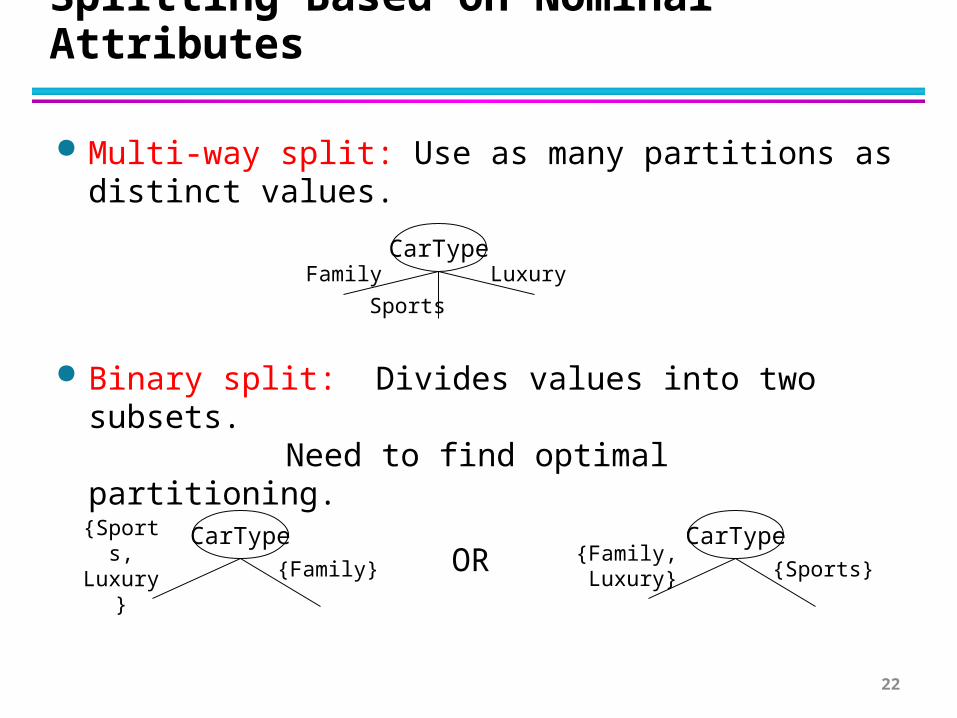
Splitting Based on Nominal Attributes
Multi-way split: Use as many partitions as distinct values.
Binary split: Divides values into two subsets. Need to find optimal partitioning.
CarTypeFamily
Sports
Luxury
CarType{Family, Luxury} {Sports}
CarType{Sports, Luxury} {Family} OR
22

Multi-way split: Use as many partitions as distinct values.
Binary split: Divides values into two subsets. Need to find optimal partitioning.
Splitting Based on Ordinal Attributes
SizeSmall
Medium
Large
Size{Medium,
Large} {Small}
Size{Small,
Medium} {Large}OR
23
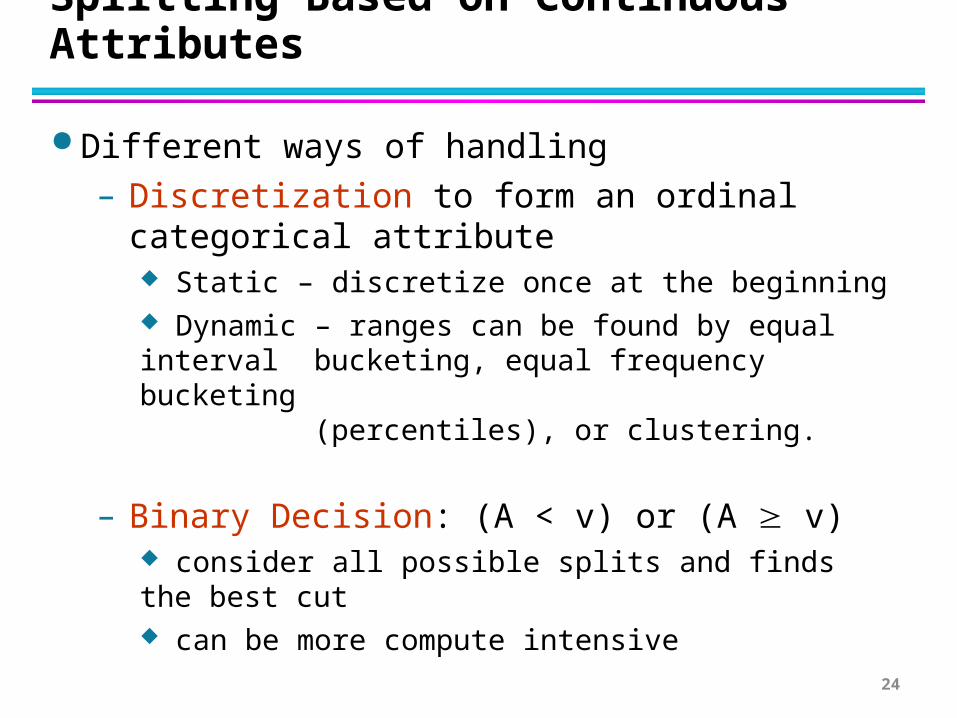
Splitting Based on Continuous Attributes
Different ways of handling
– Discretization to form an ordinal categorical attribute Static – discretize once at the beginning Dynamic – ranges can be found by equal interval
bucketing, equal frequency bucketing
(percentiles), or clustering.
– Binary Decision: (A < v) or (A v) consider all possible splits and finds the best cut can be more compute intensive
24

Splitting Based on Continuous Attributes
TaxableIncome> 80K?
Yes No
TaxableIncome?
(i) Binary split (ii) Multi-way split
< 10K
[10K,25K) [25K,50K) [50K,80K)
> 80K
25
Tree Induction
Greedy strategy.
– Split the records based on an attribute test that optimizes certain criterion.
Issues
– Determine how to split the recordsHow to specify the attribute test condition?How to determine the best split?
– Determine when to stop splitting
26

How to determine the Best Split
OwnCar?
C0: 6C1: 4
C0: 4C1: 6
C0: 1C1: 3
C0: 8C1: 0
C0: 1C1: 7
CarType?
C0: 1C1: 0
C0: 1C1: 0
C0: 0C1: 1
StudentID?
...
Yes No Family
Sports
Luxury c1c10
c20
C0: 0C1: 1
...
c11
Before Splitting: 10 records of class 0,10 records of class 1
Which test condition is the best?
27
How to determine the Best Split
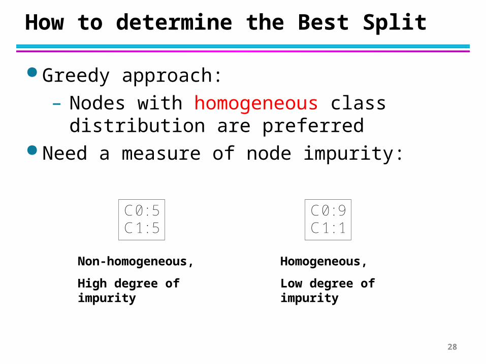
Greedy approach:
– Nodes with homogeneous class distribution are preferred
Need a measure of node impurity:
C0: 5C1: 5
C0: 9C1: 1
Non-homogeneous,
High degree of impurity
Homogeneous,
Low degree of impurity
28
Measures of Node Impurity
Gini Index
Entropy
Misclassification error
29

Measure of Impurity: GINI index
Gini Index for a given node t :
(NOTE: p( j | t) is the relative frequency of class j at node t).
– Maximum (1 - 1/nc) when records are equally distributed among all classes, implying least interesting information
– Minimum (0.0) when all records belong to one class, implying most interesting information
C1 0C2 6
Gini=0.000
C1 2C2 4
Gini=0.444
C1 3C2 3
Gini=0.500
C1 1C2 5
Gini=0.278
31
j
tjptGINI 2)]|([1)(index
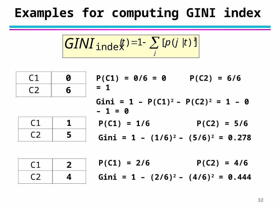
Examples for computing GINI index
C1 0 C2 6
C1 2 C2 4
C1 1 C2 5
P(C1) = 0/6 = 0 P(C2) = 6/6 = 1
Gini = 1 – P(C1)2 – P(C2)2 = 1 – 0 – 1 = 0
P(C1) = 1/6 P(C2) = 5/6
Gini = 1 – (1/6)2 – (5/6)2 = 0.278
P(C1) = 2/6 P(C2) = 4/6
Gini = 1 – (2/6)2 – (4/6)2 = 0.444
32
j
tjptGINI 2)]|([1)(index

Splitting Based on GINI split
Used in CART, SLIQ, SPRINT. When a node p is split into k partitions (children), the
quality of split is computed as,
where, ni = number of records at child i,
n = number of records at node p.
k
iindex
isplit i
n
nGINI GINI
1
)(
33
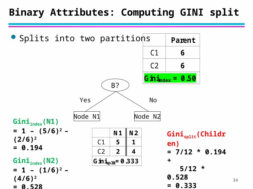
Binary Attributes: Computing GINI split
Splits into two partitions
B?
Yes No
Node N1 Node N2
Parent
C1 6
C2 6
Giniindex = 0.50
N1 N2 C1 5 1
C2 2 4
Ginisplit=0.333
Giniindex(N1) = 1 – (5/6)2 – (2/6)2 = 0.194
Giniindex(N2) = 1 – (1/6)2 – (4/6)2 = 0.528
Ginisplit(Children) = 7/12 * 0.194 + 5/12 * 0.528= 0.333
34

Categorical Attributes: Computing Gini Index
For each distinct value, gather counts for each class in the dataset
Use the count matrix to make decisions
CarType{Sports,Luxury}
{Family}
C1 3 1
C2 2 4
Gini 0.400
CarType
{Sports}{Family,Luxury}
C1 2 2
C2 1 5
Gini 0.419
CarType
Family Sports Luxury
C1 1 2 1
C2 4 1 1
Gini 0.393
Multi-way split Two-way split (find best partition of values)
35
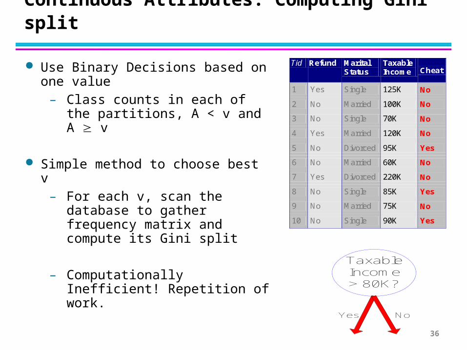
Continuous Attributes: Computing Gini split
Use Binary Decisions based on one value
– Class counts in each of the partitions, A < v and A v
Simple method to choose best v– For each v, scan the database to
gather frequency matrix and compute its Gini split
– Computationally Inefficient! Repetition of work.
TaxableIncome> 80K?
Yes No
36
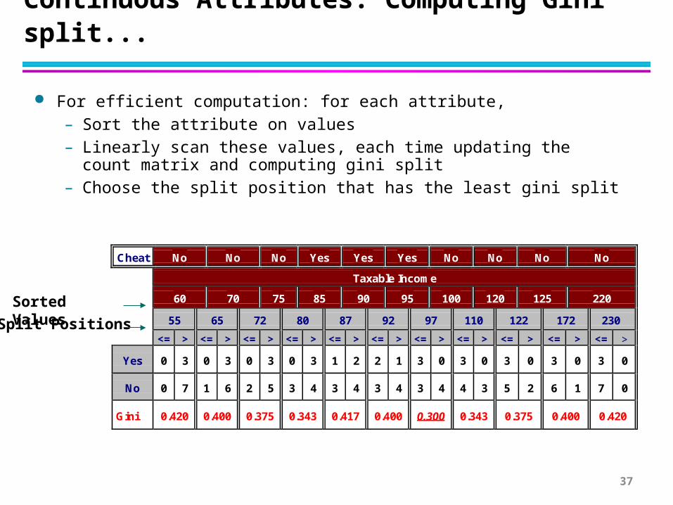
Continuous Attributes: Computing Gini split...
For efficient computation: for each attribute,– Sort the attribute on values– Linearly scan these values, each time updating the count matrix and
computing gini split– Choose the split position that has the least gini split
Cheat No No No Yes Yes Yes No No No No
Taxable Income
60 70 75 85 90 95 100 120 125 220
55 65 72 80 87 92 97 110 122 172 230
<= > <= > <= > <= > <= > <= > <= > <= > <= > <= > <= >
Yes 0 3 0 3 0 3 0 3 1 2 2 1 3 0 3 0 3 0 3 0 3 0
No 0 7 1 6 2 5 3 4 3 4 3 4 3 4 4 3 5 2 6 1 7 0
Gini 0.420 0.400 0.375 0.343 0.417 0.400 0.300 0.343 0.375 0.400 0.420
Split Positions
Sorted Values
37
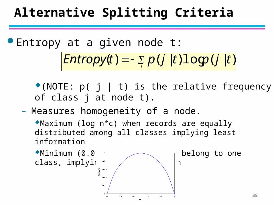
Alternative Splitting Criteria
Entropy at a given node t:
(NOTE: p( j | t) is the relative frequency of class j at node t).
– Measures homogeneity of a node. Maximum (log n*c) when records are equally distributed among all classes implying least informationMinimum (0.0) when all records belong to one class, implying most information
j
tjptjptEntropy )|(log)|()(
38
Splitting Based on INFORMATION GAIN
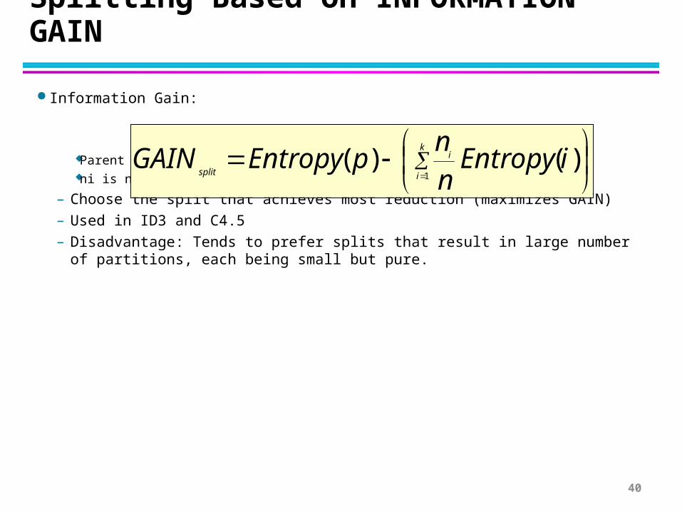
Information Gain:
Parent Node, p is split into k partitions;ni is number of records in partition I
– Choose the split that achieves most reduction (maximizes GAIN)
– Used in ID3 and C4.5
– Disadvantage: Tends to prefer splits that result in large number of partitions, each being small but pure.
k
i
i
splitiEntropy
nn
pEntropyGAIN1
)()(
40

Tree Induction
Greedy strategy.
– Split the records based on an attribute test that optimizes certain criterion.
Issues
– Determine how to split the recordsHow to specify the attribute test condition?How to determine the best split?
– Determine when to stop splitting
45
Stopping Criteria for Tree Induction
Stop expanding a node when all the records belong to the same class
Stop expanding a node when all the records have similar attribute values
Early termination (to be discussed later)
46
Decision Tree Based Classification
Advantages:
– Inexpensive to construct
– Extremely fast at classifying unknown records
– Easy to interpret for small-sized trees
– Accuracy is comparable to other classification techniques for many simple data sets
47
Example: C4.5
Uses Information Gain Sorts Continuous Attributes at each node. Needs entire data to fit in memory. Unsuitable for Large Datasets.
You can download the software from:http://www.cse.unsw.edu.au/~quinlan/c4.5r8.tar.gz
48
Practical Issues of Classification
Model Evaluation
Underfitting and Overfitting
Missing Values
49

Estimating Errors of Models (1/2)
Re-substitution errors: error on training ( e(t) )
Generalization errors: error on testing ( e’(t))
Methods for estimating generalization errors:– Optimistic approach: e’(t) = e(t)– Pessimistic approach:
For each leaf node: e’(t) = (e(t)+0.5) Total errors: e’(T) = e(T) + N 0.5 (N: number of leaf nodes) For a tree with 30 leaf nodes and 10 errors on training (out of 1000 instances): Training error = 10/1000 = 1% Generalization error = (10 + 300.5)/1000 = 2.5%
50
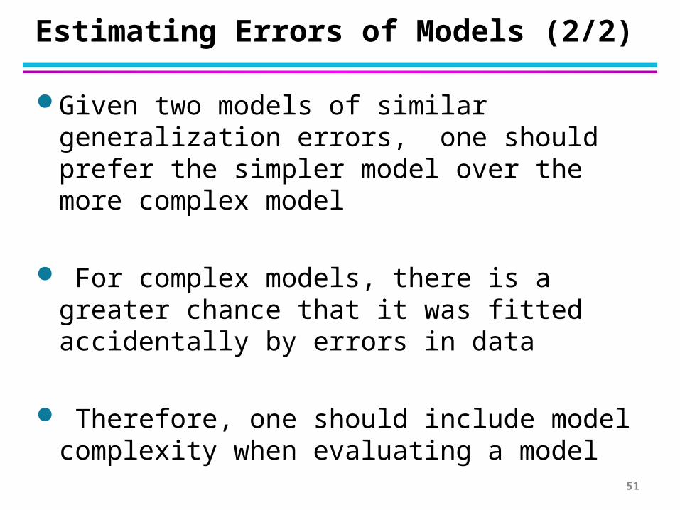
Estimating Errors of Models (2/2)
Given two models of similar generalization errors, one should prefer the simpler model over the more complex model
For complex models, there is a greater chance that it was fitted accidentally by errors in data
Therefore, one should include model complexity when evaluating a model
51
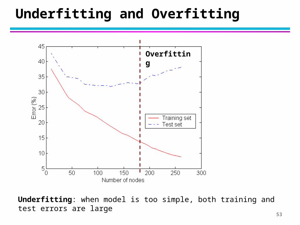
Underfitting and Overfitting
Overfitting
Underfitting: when model is too simple, both training and test errors are large
53

Overfitting due to Noise
Decision boundary is distorted by noise point
54
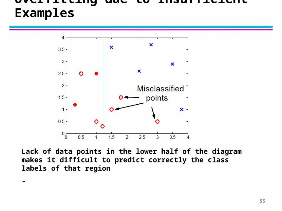
Overfitting due to Insufficient Examples
Lack of data points in the lower half of the diagram makes it difficult to predict correctly the class labels of that region
-
55

Notes on Overfitting
Overfitting results in decision trees that are more complex than necessary
Training error no longer provides a good estimate of how well the tree will perform on previously unseen records
Need new ways for estimating errors
56

How to Address Overfitting
Pre-Pruning (Early Stopping Rule)
– Stop the algorithm before it becomes a fully-grown tree
– Typical stopping conditions for a node: Stop if all instances belong to the same class Stop if all the attribute values are the same
– More restrictive conditions: Stop if number of instances is less than some user-specified threshold
Stop if expanding the current node does not improve impurity measures (e.g., Gini or information gain).
57

How to Address Overfitting…
Post-pruning
– Grow decision tree to its entirety
– Trim the nodes of the decision tree in a bottom-up fashion
– If generalization error improves after trimming, replace sub-tree by a leaf node.
– Class label of leaf node is determined from majority class of instances in the sub-tree
58

Example of Post-Pruning
A?
A1
A2 A3
A4
Class = Yes 20
Class = No 10
Error = 10/30
Training Error (Before splitting) = 10/30
Pessimistic error = (10 + 0.5)/30 = 10.5/30
Training Error (After splitting) = 9/30
Pessimistic error (After splitting)
= (9 + 4 0.5)/30 = 11/30
PRUNE!
Class = Yes 8
Class = No 4
Class = Yes 3
Class = No 4
Class = Yes 4
Class = No 1
Class = Yes 5
Class = No 1
59
Error = 9/30
Handling Missing Attribute Values
Missing values affect decision tree construction :
– Affects how impurity measures are computed
– Affects how a test instance with missing value is classified
60
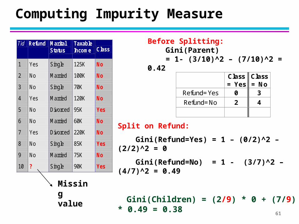
Computing Impurity Measure
Tid Refund Marital Status
Taxable Income Class
1 Yes Single 125K No
2 No Married 100K No
3 No Single 70K No
4 Yes Married 120K No
5 No Divorced 95K Yes
6 No Married 60K No
7 Yes Divorced 220K No
8 No Single 85K Yes
9 No Married 75K No
10 ? Single 90K Yes 10
Class = Yes
Class = No
Refund=Yes 0 3
Refund=No 2 4
Split on Refund:
Gini(Refund=Yes) = 1 – (0/2)^2 – (2/2)^2 = 0
Gini(Refund=No) = 1 - (3/7)^2 – (4/7)^2 = 0.49
Gini(Children) = (2/9) * 0 + (7/9) * 0.49 = 0.38 Missing value
Before Splitting: Gini(Parent) = 1- (3/10)^2 – (7/10)^2 = 0.42
61
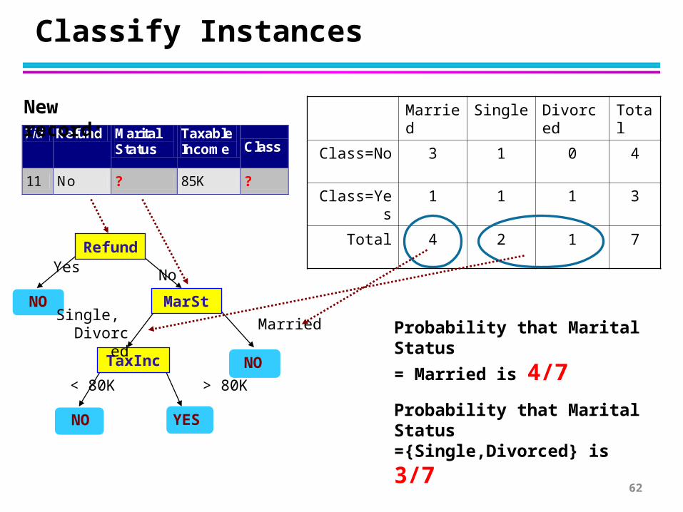
Classify Instances
Refund
MarSt
TaxInc
YESNO
NO
NO
Yes No
Married Single,
Divorced
< 80K > 80K
Married Single Divorced Total
Class=No 3 1 0 4
Class=Yes 1 1 1 3
Total 4 2 1 7
Tid Refund Marital Status
Taxable Income Class
11 No ? 85K ? 10
New record:
Probability that Marital Status
= Married is 4/7
Probability that Marital Status
={Single,Divorced} is 3/7
62
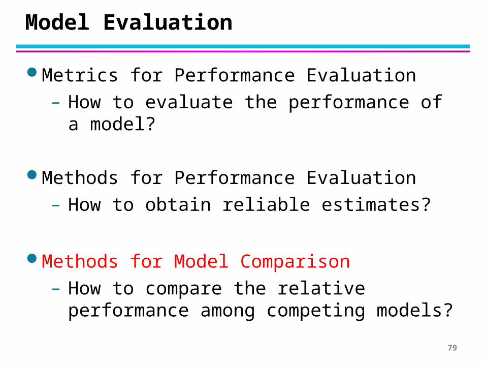
Model Evaluation
Metrics for Performance Evaluation
– How to evaluate the performance of a model?
Methods for Performance Evaluation
– How to obtain reliable estimates?
Methods for Model Comparison
– How to compare the relative performance among competing models?
67
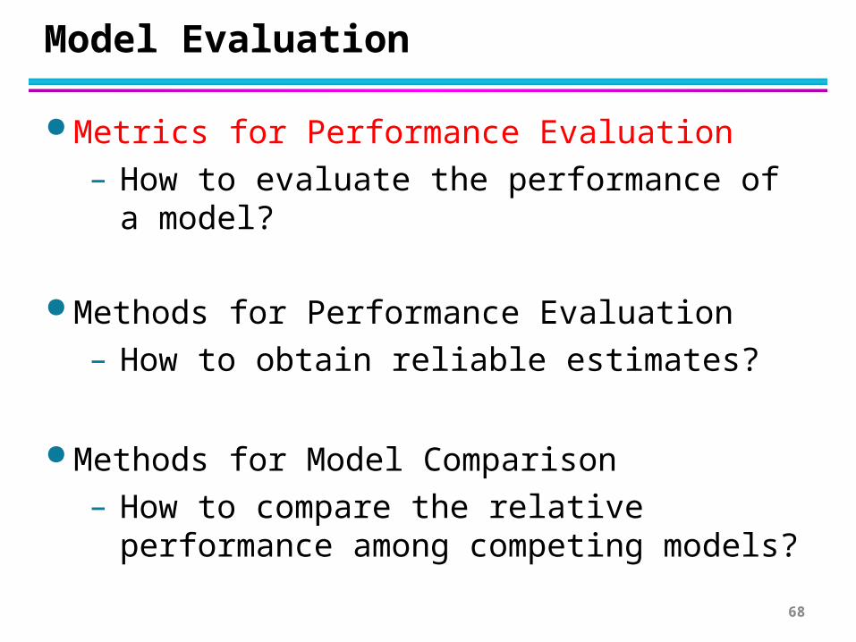
Model Evaluation
Metrics for Performance Evaluation
– How to evaluate the performance of a model?
Methods for Performance Evaluation
– How to obtain reliable estimates?
Methods for Model Comparison
– How to compare the relative performance among competing models?
68
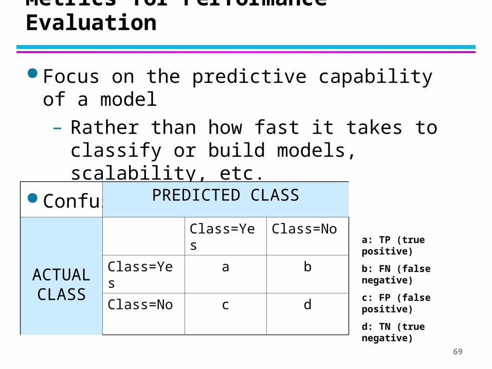
Metrics for Performance Evaluation
Focus on the predictive capability of a model
– Rather than how fast it takes to classify or build models, scalability, etc.
Confusion Matrix:
PREDICTED CLASS
ACTUALCLASS
Class=Yes Class=No
Class=Yes a b
Class=No c d
a: TP (true positive)
b: FN (false negative)
c: FP (false positive)
d: TN (true negative)
69
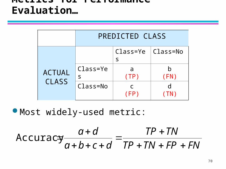
Metrics for Performance Evaluation…
Most widely-used metric:
PREDICTED CLASS
ACTUALCLASS
Class=Yes Class=No
Class=Yes a(TP)
b(FN)
Class=No c(FP)
d(TN)
FNFPTNTPTNTP
dcbada
Accuracy
70
Limitation of Accuracy
Consider a 2-class problem
– Number of Class 0 examples = 9990
– Number of Class 1 examples = 10
If model predicts everything to be class 0, accuracy is 9990/10000 = 99.9 %
– Accuracy is misleading because model does not detect any class 1 example
71

Cost Matrix
PREDICTED CLASS
ACTUALCLASS
C(i|j) Class=Yes Class=No
Class=Yes C(Yes|Yes) C(No|Yes)
Class=No C(Yes|No) C(No|No)
C(i|j): Cost of misclassifying class j example as class i
72

Computing Cost of Classification
Cost Matrix
PREDICTED CLASS
ACTUALCLASS
C(i|j) + -
+ -1 100
- 1 0
Model M1 PREDICTED CLASS
ACTUALCLASS
+ -
+ 150 40
- 60 250
Model M2 PREDICTED CLASS
ACTUALCLASS
+ -
+ 250 45
- 5 200
Accuracy = 80%
Cost = 3910
Accuracy = 90%
Cost = 4255
73
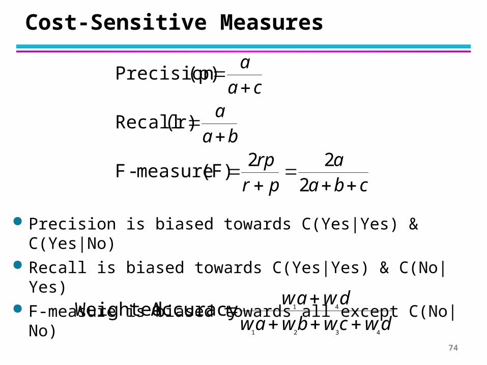
Cost-Sensitive Measures
cbaa
prrp
baa
caa
222
(F) measure-F
(r) Recall
(p)Precision
Precision is biased towards C(Yes|Yes) & C(Yes|No) Recall is biased towards C(Yes|Yes) & C(No|Yes) F-measure is biased towards all except C(No|No)
dwcwbwawdwaw
4321
41Accuracy Weighted
74
Model Evaluation
Metrics for Performance Evaluation
– How to evaluate the performance of a model?
Methods for Performance Evaluation
– How to obtain reliable estimates?
Methods for Model Comparison
– How to compare the relative performance among competing models?
75
Methods for Performance Evaluation
How to obtain a reliable estimate of performance?
Performance of a model may depend on other factors besides the learning algorithm:
– Class distribution
– Cost of misclassification
– Size of training and test sets
76
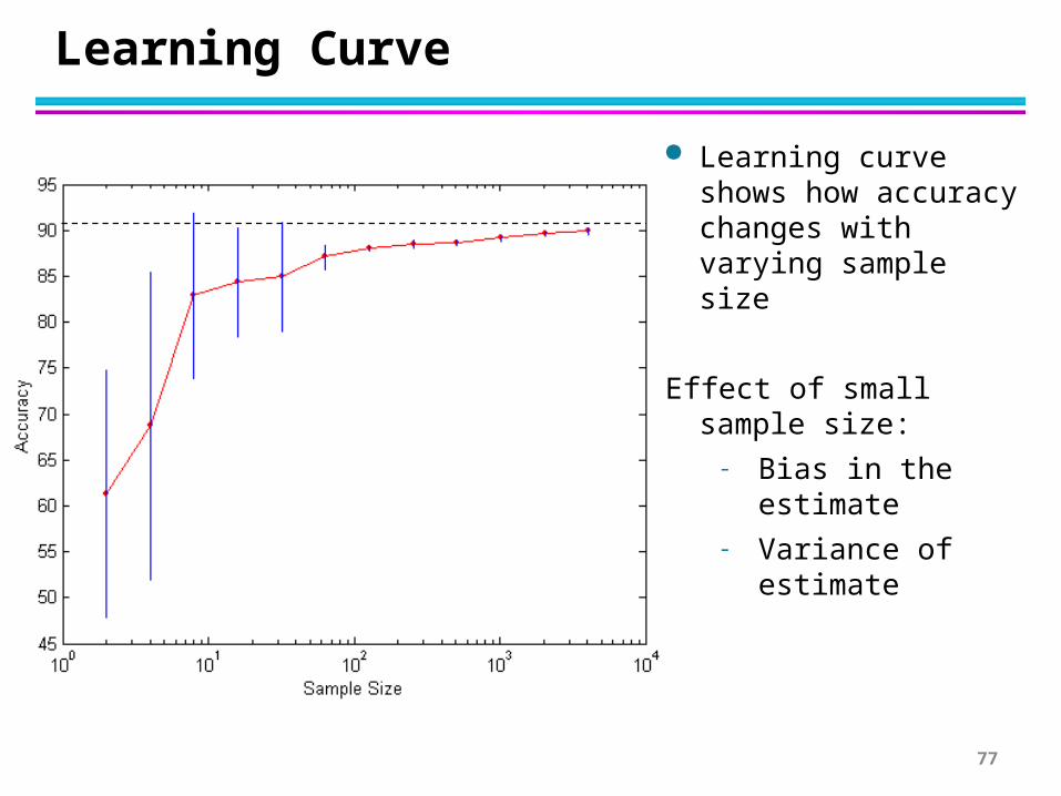
Learning Curve
Learning curve shows how accuracy changes with varying sample size
Effect of small sample size:- Bias in the estimate- Variance of estimate
77

Methods of Estimation
Holdout– Reserve 2/3 for training and 1/3 for testing
Random subsampling– Repeated holdout
Cross validation– Partition data into k disjoint subsets– k-fold: train on k-1 partitions, test on the
remaining one– Leave-one-out: k=n
Bootstrap– Sampling with replacement
78
Model Evaluation
Metrics for Performance Evaluation
– How to evaluate the performance of a model?
Methods for Performance Evaluation
– How to obtain reliable estimates?
Methods for Model Comparison
– How to compare the relative performance among competing models?
79

ROC (Receiver Operating Characteristic)
Characterize the trade-off between positive hits and false alarms
ROC curve plots TP (on the y-axis) against FP (on the x-axis)
80
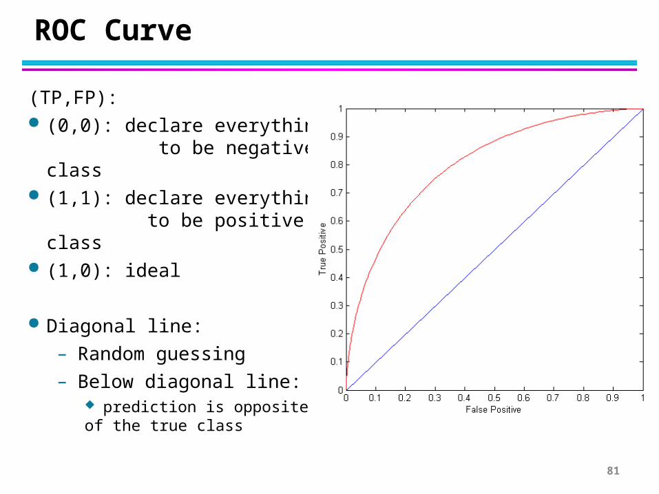
ROC Curve
(TP,FP): (0,0): declare everything
to be negative class (1,1): declare everything
to be positive class (1,0): ideal
Diagonal line:
– Random guessing
– Below diagonal line: prediction is opposite of the true class
81

How to Construct an ROC curve
Instance P(+|A) True Class
1 0.95 +
2 0.93 +
3 0.87 -
4 0.85 -
5 0.85 -
6 0.85 +
7 0.76 -
8 0.53 +
9 0.43 -
10 0.25 +
• Use classifier that produces posterior probability for each test instance P(+|A)
• Sort the instances according to P(+|A) in decreasing order
• Apply threshold at each unique value of P(+|A)
• Count the number of TP, FP,
TN, FN at each threshold
• TP rate, TPR = TP/(TP+FN)
• FP rate, FPR = FP/(FP + TN)82
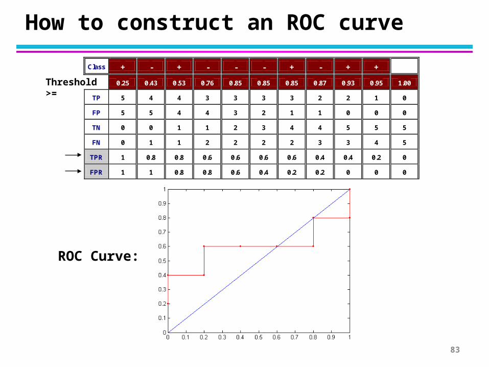
How to construct an ROC curve
Class + - + - - - + - + +
P 0.25 0.43 0.53 0.76 0.85 0.85 0.85 0.87 0.93 0.95 1.00
TP 5 4 4 3 3 3 3 2 2 1 0
FP 5 5 4 4 3 2 1 1 0 0 0
TN 0 0 1 1 2 3 4 4 5 5 5
FN 0 1 1 2 2 2 2 3 3 4 5
TPR 1 0.8 0.8 0.6 0.6 0.6 0.6 0.4 0.4 0.2 0
FPR 1 1 0.8 0.8 0.6 0.4 0.2 0.2 0 0 0
Threshold >=
ROC Curve:
83
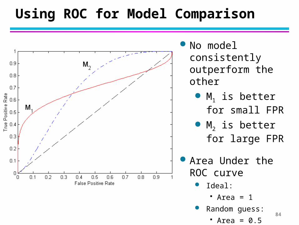
Using ROC for Model Comparison
No model consistently outperform the other M1 is better for
small FPR M2 is better for
large FPR
Area Under the ROC curve
Ideal: Area = 1
Random guess: Area = 0.5
84
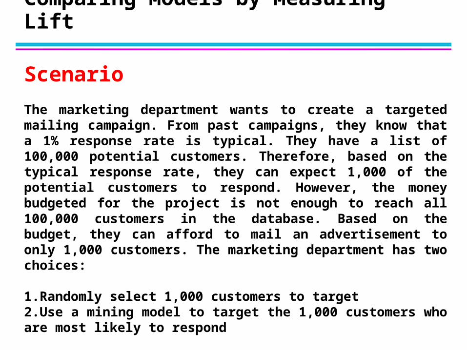
Comparing Models by Measuring Lift
Scenario
The marketing department wants to create a targeted mailing campaign. From past campaigns, they know that a 1% response rate is typical. They have a list of 100,000 potential customers. Therefore, based on the typical response rate, they can expect 1,000 of the potential customers to respond. However, the money budgeted for the project is not enough to reach all 100,000 customers in the database. Based on the budget, they can afford to mail an advertisement to only 1,000 customers. The marketing department has two choices:
1.Randomly select 1,000 customers to target2.Use a mining model to target the 1,000 customers who are most likely to respond
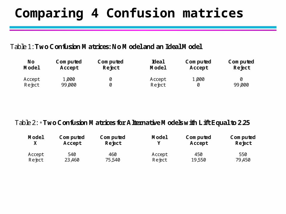
Table 1: Two Confusion Matrices: No Model and an Ideal Model
No Computed Computed Ideal Computed Computed Model Accept Reject Model Accept Reject
Accept 1,000 0 Accept 1,000 0 Reject 99,000 0 Reject 0 99,000
Table 2: • Two Confusion Matrices for Alternative Models with Lift Equal to 2.25
Model Computed Computed Model Computed Computed X Accept Reject Y Accept Reject
Accept 540 460 Accept 450 550 Reject 23,460 75,540 Reject 19,550 79,450
Comparing 4 Confusion matrices

Comparing Models by Measuring Lift
25.2100000/1000
24000/540)( XModelLift
25.2100000/1000
20000/450)( YModelLift
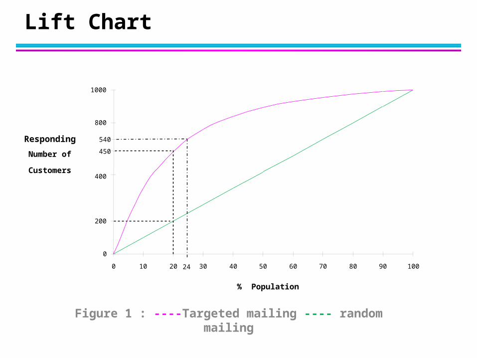
Figure 1 : ----Targeted mailing ---- random mailing
Lift Chart
0
200
400
450
800
1000
0 10 20 30 40 50 60 70 80 90 100
Number of
Customers
Responding
% Population
540
24
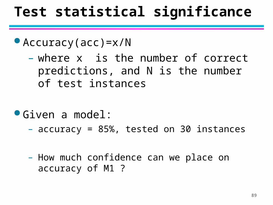
Test statistical significance
Accuracy(acc)=x/N
– where x is the number of correct predictions, and N is the number of test instances
Given a model:– accuracy = 85%, tested on 30 instances
– How much confidence can we place on accuracy of M1 ?
89

Confidence Interval for Accuracy
For test sets (N > 30) – acc follows a normal
distribution with mean μ
and variance μ(1- μ)/N.
The confidence interval
for acc is:
1)/)1(
( 2/12/ ZN
μaccZP
Area = 1 -
Z/2 Z1- /2
)(2
4422
2/
222/
22/
ZN
accNaccNZZaccN
90
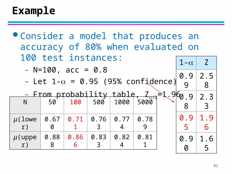
Example
Consider a model that produces an accuracy of 80% when evaluated on 100 test instances:– N=100, acc = 0.8
– Let 1- = 0.95 (95% confidence)
– From probability table, Z/2=1.96
1- Z
0.99 2.58
0.98 2.33
0.95 1.96
0.90 1.65
N 50 100 500 1000 5000
μ(lower) 0.670 0.711 0.763 0.774 0.789
μ(upper) 0.888 0.866 0.833 0.824 0.811
91
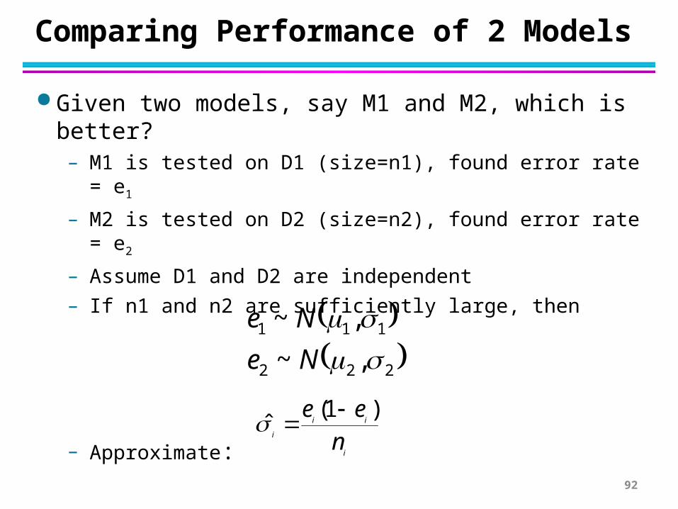
Comparing Performance of 2 Models
Given two models, say M1 and M2, which is better?– M1 is tested on D1 (size=n1), found error rate = e1
– M2 is tested on D2 (size=n2), found error rate = e2
– Assume D1 and D2 are independent
– If n1 and n2 are sufficiently large, then
– Approximate:
222
111
,~
,~
Ne
Ne
i
ii
i nee )1(
ˆ
92
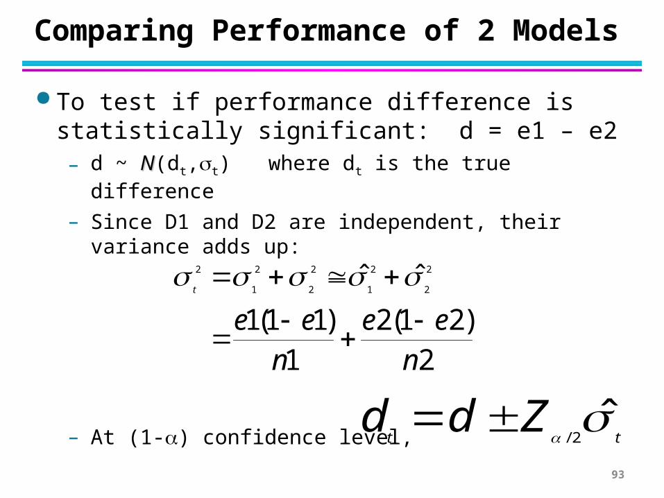
Comparing Performance of 2 Models
To test if performance difference is statistically significant: d = e1 – e2– d ~ NN(dt,t) where dt is the true difference
– Since D1 and D2 are independent, their variance adds up:
– At (1-) confidence level,
2)21(2
1)11(1
ˆˆ 2
2
2
1
2
2
2
1
2
nee
nee
t
ttZdd
ˆ
2/
93
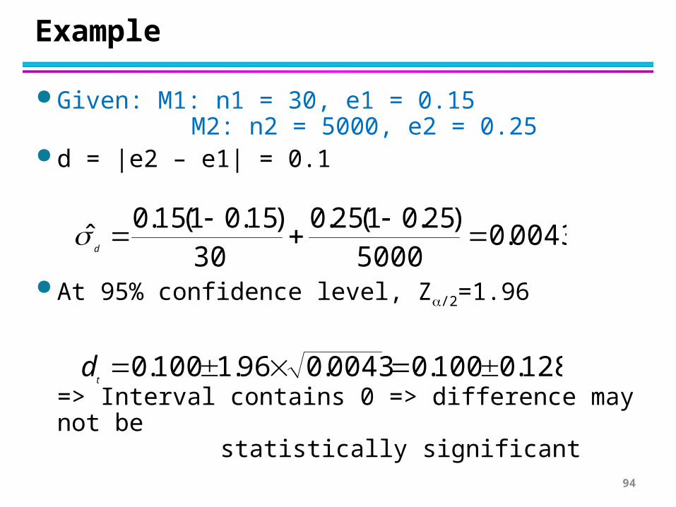
Example
Given: M1: n1 = 30, e1 = 0.15 M2: n2 = 5000, e2 = 0.25
d = |e2 – e1| = 0.1
At 95% confidence level, Z/2=1.96
=> Interval contains 0 => difference may not be statistically significant
0043.05000
)25.01(25.030
)15.01(15.0ˆ
d
128.0100.00043.096.1100.0 t
d
94


