


COLORING PROBLEMS
by
Thomas Antonio Charles Chartier
A thesis
submitted in partial fulfillment
of the requirements for the degree of
Master of Science in Mathematics
Boise State University
December 2011
© 2011Thomas Antonio Charles Chartier
ALL RIGHTS RESERVED
BOISE STATE UNIVERSITY GRADUATE COLLEGE
DEFENSE COMMITTEE AND FINAL READING APPROVALS
of the thesis submitted by
Thomas Antonio Charles Chartier
Thesis Title: Coloring Problems
Date of Final Oral Examination: 13 October 2011
The following individuals read and discussed the thesis submitted by student ThomasAntonio Charles Chartier, and they evaluated his presentation and response to ques-tions during the final oral examination. They found that the student passed the finaloral examination.
Andres E. Caicedo, Ph.D. Chair
Jens Harlander, Ph.D. Member, Supervisory Committee
Marion Scheepers, Ph.D. Member, Supervisory Committee
The final reading approval of the thesis was granted by Andres E. Caicedo, Ph.D.,Chair. The thesis was approved for the Graduate College by John R. Pelton, Ph.D.,Dean of the Graduate College.
Dedicated to Bethany, Parker, and Daxton
iv

ACKNOWLEDGMENTS
I would like to thank Dr. Andres Caicedo for his patience and support through
the entire thesis process. I would also like to express my gratitude to the following:
The Boise State University Mathematics department for providing me with a teaching
assistantship, Dr. Jens Harlander and Dr. Marion Scheepers for serving as committee
members, Dr. Zach Teitler for informing us of several relevant references and Dr.
Rodney Forcade for sharing with us his relevant works and data. Lastly, I would like
to say thank you to Bethany, I certainly could not have done this without you.
v
ABSTRACT
This thesis considers several coloring problems all of which have a combinatorial
flavor. We review some results on the chromatic number of the plane, and improve
a bound on the value of regressive Ramsey numbers. The main work of this thesis
considers the problem of whether given any n ≥ 1, one can color Z+ in such a way that
for all a ∈ Z+ the numbers a,2a,3a, ..., na are assigned different colors. Such colorings
are referred to as satisfactory. We provide a sufficient condition for guaranteeing
the existence of satisfactory colorings and analyze the resulting structure. Explicit
constructions are given for n ≤ 54. The thesis concludes with some suggestions towards
a general argument.
vi
TABLE OF CONTENTS
ABSTRACT . . . . . . . . . . . . . . . . . . . . . . . . . . . . . . . . . . . . . . . . . . . . . . . . . . vi
LIST OF TABLES . . . . . . . . . . . . . . . . . . . . . . . . . . . . . . . . . . . . . . . . . . . . . x
LIST OF FIGURES . . . . . . . . . . . . . . . . . . . . . . . . . . . . . . . . . . . . . . . . . . . . xii
LIST OF SYMBOLS . . . . . . . . . . . . . . . . . . . . . . . . . . . . . . . . . . . . . . . . . . . xiii
1 INTRODUCTION . . . . . . . . . . . . . . . . . . . . . . . . . . . . . . . . . . . . . . . . . . 1
1.1 History of Coloring . . . . . . . . . . . . . . . . . . . . . . . . . . . . . . . . . . . . . . . . . . . 1
1.2 Necessary Background . . . . . . . . . . . . . . . . . . . . . . . . . . . . . . . . . . . . . . . . . 3
1.2.1 Linear Congruences . . . . . . . . . . . . . . . . . . . . . . . . . . . . . . . . . . . . . 3
1.2.2 Power Residues . . . . . . . . . . . . . . . . . . . . . . . . . . . . . . . . . . . . . . . . 5
1.2.3 Principal Number Theoretic Results . . . . . . . . . . . . . . . . . . . . . . . 7
1.2.4 Cardinality . . . . . . . . . . . . . . . . . . . . . . . . . . . . . . . . . . . . . . . . . . . . 9
2 THE CHROMATIC NUMBER OF THE PLANE . . . . . . . . . . . . . . . 16
3 REGRESSIVE FUNCTIONS ON PAIRS . . . . . . . . . . . . . . . . . . . . . . 24
4 SATISFACTORY COLORINGS . . . . . . . . . . . . . . . . . . . . . . . . . . . . . . 26
4.1 The Problem . . . . . . . . . . . . . . . . . . . . . . . . . . . . . . . . . . . . . . . . . . . . . . . . 26
4.2 An Example . . . . . . . . . . . . . . . . . . . . . . . . . . . . . . . . . . . . . . . . . . . . . . . . . 27
4.3 The Core . . . . . . . . . . . . . . . . . . . . . . . . . . . . . . . . . . . . . . . . . . . . . . . . . . . 30
vii
5 STRONG REPRESENTATIONS . . . . . . . . . . . . . . . . . . . . . . . . . . . . . 36
5.1 Strong Representatives . . . . . . . . . . . . . . . . . . . . . . . . . . . . . . . . . . . . . . . . 36
5.1.1 Trivial Representatives . . . . . . . . . . . . . . . . . . . . . . . . . . . . . . . . . . 38
5.2 Satisfactory Colorings with n ≤ 5 . . . . . . . . . . . . . . . . . . . . . . . . . . . . . . . . 40
5.2.1 Density of Strong Representatives . . . . . . . . . . . . . . . . . . . . . . . . . 44
5.3 k-representatives . . . . . . . . . . . . . . . . . . . . . . . . . . . . . . . . . . . . . . . . . . . . . 46
5.3.1 kn-densities . . . . . . . . . . . . . . . . . . . . . . . . . . . . . . . . . . . . . . . . . . . 56
5.4 Multiplicative Colorings . . . . . . . . . . . . . . . . . . . . . . . . . . . . . . . . . . . . . . . 58
5.5 Partial G-Homomorphisms . . . . . . . . . . . . . . . . . . . . . . . . . . . . . . . . . . . . . 62
5.5.1 An Example . . . . . . . . . . . . . . . . . . . . . . . . . . . . . . . . . . . . . . . . . . . 66
6 MULTIPLICATIVE COLORINGS WITH AT MOST 8 COLORS. 68
6.1 Six Colors . . . . . . . . . . . . . . . . . . . . . . . . . . . . . . . . . . . . . . . . . . . . . . . . . . . 68
6.2 Seven Colors . . . . . . . . . . . . . . . . . . . . . . . . . . . . . . . . . . . . . . . . . . . . . . . . . 71
6.3 Eight Colors . . . . . . . . . . . . . . . . . . . . . . . . . . . . . . . . . . . . . . . . . . . . . . . . . 74
7 FINAL REMARKS . . . . . . . . . . . . . . . . . . . . . . . . . . . . . . . . . . . . . . . . . 82
7.1 A Conjecture of R.L. Graham . . . . . . . . . . . . . . . . . . . . . . . . . . . . . . . . . . 82
7.2 A Late Conclusion . . . . . . . . . . . . . . . . . . . . . . . . . . . . . . . . . . . . . . . . . . . . 90
REFERENCES . . . . . . . . . . . . . . . . . . . . . . . . . . . . . . . . . . . . . . . . . . . . . . . . 93
A CODE . . . . . . . . . . . . . . . . . . . . . . . . . . . . . . . . . . . . . . . . . . . . . . . . . . . . . 95
A.1 Matlab Code for g(4,4) . . . . . . . . . . . . . . . . . . . . . . . . . . . . . . . . . . . . . . . . 95
A.2 The Search for Strong Representatives . . . . . . . . . . . . . . . . . . . . . . . . . . . 106
A.3 Density Data Collection Code for Strong Representatives of Order 5 . . 106
A.4 Density Data Collection Code for 3-representatives . . . . . . . . . . . . . . . . . 109
viii
B PARTIAL HOMOMORPHISM TABLES . . . . . . . . . . . . . . . . . . . . . . 113
C GROUPLESS n . . . . . . . . . . . . . . . . . . . . . . . . . . . . . . . . . . . . . . . . . . . . . 117
ix
LIST OF TABLES
5.1 Smallest strong representative p = nk + 1 of order n for n ≤ 33. . . . . . . . 39
5.2 4m-representatives. . . . . . . . . . . . . . . . . . . . . . . . . . . . . . . . . . . . . . . . . . . 49
5.3 A Z6-satisfactory group. . . . . . . . . . . . . . . . . . . . . . . . . . . . . . . . . . . . . . . 64
6.1 The base operation table for n = 6. . . . . . . . . . . . . . . . . . . . . . . . . . . . . . . 69
6.2 The associated Z6-coloring is strongly represented by 103 = 6 ⋅ 17 + 1. . 70
6.3 The associated Z6-coloring is strongly represented by 7 = 6 ⋅ 1 + 1. . . . . 70
6.4 The associated Z6-coloring is strongly represented by 487 = 6 ⋅ 81 + 1. . 71
6.5 The associated Z6-coloring is strongly represented by 547 = 6 ⋅ 91 + 1. . 71
6.6 The associated Z6-coloring is strongly represented by 13 = 6 ⋅ 2 + 1. . . . 72
6.7 Base operation table for n = 7. . . . . . . . . . . . . . . . . . . . . . . . . . . . . . . . . . 72
6.8 The associated Z7-coloring is strongly represented by 2087 = 7 ⋅ 298 + 1. 73
6.9 The associated Z7-coloring is strongly represented by 1429 = 7 ⋅ 204 + 1. 73
6.10 The associated Z7-coloring is strongly represented by 659 = 7 ⋅ 94 + 1. . 74
6.11 The associated Z7-coloring is strongly represented by 21911 = 7 ⋅3130+1. 74
6.12 The associated Z7-coloring is strongly represented by 3557 = 7 ⋅ 508 + 1. 75
6.13 The associated Z7-coloring is strongly represented by 17431 = 7 ⋅2490+1. 75
6.14 The base operation table for n = 8. . . . . . . . . . . . . . . . . . . . . . . . . . . . . . 76
6.15 Z8-coloring corresponding to the sequence (1,5,3,7). . . . . . . . . . . . . . . 77
6.16 Z8-coloring corresponding to the sequence (1,7,5,3). . . . . . . . . . . . . . . 77
6.17 Z8-coloring corresponding to the sequence (3,1,5,7). . . . . . . . . . . . . . . 77
x
6.18 Z8-coloring corresponding to the sequence (3,7,1,5). . . . . . . . . . . . . . . 78
6.19 Z8-coloring corresponding to the sequence (7,1,3,5). . . . . . . . . . . . . . . 78
6.20 Z8-coloring corresponding to the sequence (7,5,1,3). . . . . . . . . . . . . . . . 78
6.21 Partial group operation corresponding to the sequence (3,7,5,1). . . . . 79
6.22 Partial group operation corresponding to the sequence (7,5,3,1). . . . . 79
6.23 Group corresponding to the sequence (3,7,5,1) ∶ a = 1, 2, 4, or 8. . . . . . 80
6.24 Group corresponding to the sequence (7,5,3,1) ∶ a = 1, 2, 4, or 8. . . . . . 80
A.1 Density data for satisfactory 5-colorings . . . . . . . . . . . . . . . . . . . . . . . . . 112
B.1 Partial Homomorphism table for n ∈ [1,16]. . . . . . . . . . . . . . . . . . . . . . . 114
B.2 Partial Homomorphism table for n ∈ [17,32]. . . . . . . . . . . . . . . . . . . . . . 115
B.3 Partial Homomorphism table for n ∈ [33,39]. . . . . . . . . . . . . . . . . . . . . . 116
B.4 Partial Homomorphism table for n ∈ [40,48]. . . . . . . . . . . . . . . . . . . . . . 116
B.5 Partial Homomorphism table for n ∈ [49,54]. . . . . . . . . . . . . . . . . . . . . . 116
C.1 A list of all groupless n for n ≤ 500. . . . . . . . . . . . . . . . . . . . . . . . . . . . . . 118
xi
LIST OF FIGURES
1.1 The desired mapping . . . . . . . . . . . . . . . . . . . . . . . . . . . . . . . . . . . . . . . . . 11
2.1 A χ coloring of an equilateral triangle of side length 1. . . . . . . . . . . . . . 17
2.2 A graph that cannot be χ colored with 3 colors. . . . . . . . . . . . . . . . . . . 18
2.3 An Hexagonal Tessellation of R2, which cannot be χ colored. . . . . . . . . 19
2.4 A graph that cannot be χ colored with 3 colors. . . . . . . . . . . . . . . . . . . 20
2.5 G1 . . . . . . . . . . . . . . . . . . . . . . . . . . . . . . . . . . . . . . . . . . . . . . . . . . . . . . . . 21
2.6 G2 . . . . . . . . . . . . . . . . . . . . . . . . . . . . . . . . . . . . . . . . . . . . . . . . . . . . . . . . 22
A.1 A Matlab function witnessing a regressive function with no min-homogeneous
set of size 4 . . . . . . . . . . . . . . . . . . . . . . . . . . . . . . . . . . . . . . . . . . . . . . . . . . 106
A.2 Maple code used in the search for strong representatives . . . . . . . . . . . . 107
A.3 Maple code used for data acquisition in the case of 5 colors . . . . . . . . . 108
A.4 Sample of the output produced by the code found in Figure A.5 when
k = 3. . . . . . . . . . . . . . . . . . . . . . . . . . . . . . . . . . . . . . . . . . . . . . . . . . . . . . . 110
A.5 Sage code used in the density analysis of k-representatives . . . . . . . . . . 111
xii
LIST OF SYMBOLS
N ................................ {0,1,2,3, ...}
Z+ ................................ {1,2,3, ...}
Q ................................ The set of rational numbers.
R ................................ The set of real numbers.
Zn ................................ The integers modulo n.
Z∗n ................................ The group of units modulo n.
(a, b) ................................ The greatest common divisor of a and b.
indg(a) ............................. The index of a with respect to the primitive root g.
π(n) ................................. The number of primes less than or equal to n.
K =Kn .............................. The n-th core.
CKn ................................. The set of satisfactory colorings of Kn.
MKn ................................. The set of multiplicative colorings of Kn.
g⊕α ................................. g ⊕⋯⊕ g´¹¹¹¹¹¹¹¹¹¹¹¹¹¹¹¹¹¸¹¹¹¹¹¹¹¹¹¹¹¹¹¹¹¹¹¶α times
, where g is an element of an abelian group.
n ................................ {1,2, . . . , n}
xiii
1
CHAPTER 1
INTRODUCTION
1.1 History of Coloring
Graph Coloring is the assignment of labels or “colors” to the edges or vertices of
a graph [6]. Problems in this area (more specifically those seeking to ascertain
the properties of a given coloring, or to determine whether colorings with specific
properties exist) have given impetus to whole fields in combinatorics (Ramsey theory,
see [10]) and set theory (partition calculus); the results often have application in
number theory and analysis, among others.
Consider the following question, originally posed by Francis Guthrie in 1852, see
[4].
Is it possible to color any planar map using four colors in such a way
that regions sharing a common boundary, excluding boundaries which are
comprised of a single point, do not share the same color?
The affirmative answer and its proof were finally attained by Kenneth Appel and
Wolfgang Haken some 124 years later with the aid of computers.1 It was during this
time that the still very active area of mathematics known as Graph Coloring came to
be.1Here it is noteworthy to mention that this was the first significant mathematical result in which
a computer was used in an essential manner. For a more detailed discussion of the result and itssubsequent impact on mathematical practice refer to Chapter 21 of [4].
2
This thesis is organized as follows.
The rest of this chapter is devoted to providing some of the necessary background
for our results.
In Chapter 2, we give a brief description of a well–known problem in graph coloring
theory, the chromatic number of the plane, and some of the results that have been
obtained.
In Chapter 3, we extend a recent result of Andres Caicedo in [9] concerning
regressive functions on pairs.
The remainder of the thesis deals with the main point of this thesis. The question
at hand is introduced in Chapter 4, and in full generality remains unsolved. It asks
for the existence of certain colorings of positive integers, generalizing a question from
KoMaL [3]. We call such colorings satisfactory. The key notion of the n-core is
introduced in Section 4.2 and discussed in detail in Section 4.3.
In Section 5.1, we give a sufficient condition, using elementary number theory,
which guarantees a satisfactory coloring exists using n colors, provided certain primes
of the form nk+1 exist. In Subsection 5.1.1, we give a solution to the question posed
in KoMaL. In Section 5.2, we identify all satisfactory colorings with at most 5 colors.
Multiplicative colorings are introduced in Section 5.4, and the associated notion of
partial G-homomorphism, for G an abelian group, is defined in Section 5.5.
In Chapter 6, we identify all multiplicative colorings with at most 8 colors.
In Chapter 7, we discuss a related problem that provides insight to the inherent
difficulty of our problem.
Also, four days after the defense of this thesis, the work of Rodney Forcade, Jack
Lamoreaux, and Andrew Pollington in [18] and Forcade and Pollington in [19] was
brought to our attention. As such, several of the problems we mention as open have
3
in fact been solved. Rather than rewriting significant portions of the entire thesis, we
devote Section 7.2 to discussing how the results in [19] and [18] pertain to our current
work and the effect they have on future considerations.
This thesis relied heavily on the use of scientific computing software. More
specifically, we used C++, Maple, Matlab, and Sage in the acquisition of data and
to some extent obtain various results throughout the thesis. As such, the main code
that has been used has been included in Appendix A.
1.2 Necessary Background
We begin by providing some number theoretic results that have been fundamental in
constructing satisfactory colorings. All of them can be found in [1]. We also establish
some basic results on the cardinality of sets.
1.2.1 Linear Congruences
Theorem 1.1. Let m,a, b be integers with m ≥ 1. Let d = (a,m) be the gcd of a and
m. The congruence
ax ≡ b (mod m) (1.1)
has solutions if and only if
b ≡ 0 (mod d).
Proof. Let d = (a,m). Congruence (1.1) has a solution if and only if there exist
x, y ∈ Z such that
ax −my = b.
4
Since d ∣a and d ∣m and d is an integer linear combination of a and m by Theorem
1.15 of [1], then ax −my = b has a solution if and only if d ∣b , i.e., b ≡ 0 (mod d).
Theorem 1.2. Let m,a, b, d be as in Theorem 1.1. If b ≡ 0 (mod d), then the
congruence (1.1) has exactly d solutions that are pairwise incongruent modulo m. In
particular, if (a,m) = 1, then for every b the congruence (1.1) has a unique solution
modulo m.
Proof. Suppose x and y are solutions to Congruence (1.1), then
a(x − y) ≡ ax − ay ≡ b − b ≡ 0 (mod m),
thus a(x − y) is a multiple of m and so for some integer z
a(x − y) =mz.
If (a,m) = d, then (a/d,m/d) = 1 and
a
d(x − y) = m
dz.
This means that m/d divides x − y and we have that
y ≡ x (modm
d).
Moreover, every integer y of this form is a solution to Congruence (1.1). An integer
congruent to x modulo m/d is congruent to x + im/d modulo m for some integer
i = 0,1,2, ..., d − 1, and the d integers x + im/d with i = 1,2,3, ..., d − 1 are pairwise
incongruent modulo m. Thus, (1.1) has exactly d pairwise incongruent solutions.
5
1.2.2 Power Residues
Let m,k, a ∈ Z be such that m ≥ 2, k ≥ 2, and (a,m) = 1. Refer to a as a kth power
residue modulo m if, and only if, there is an x ∈ Z such that
xk ≡ a (mod m).
The order of a modulo m is the smallest integer d such that ad ≡ 1 (mod m).
Definition 1.3. Recall that the Euler totient function φ(n) counts the number of
positive integers less than or equal to n that are relatively prime to n. The number a
is a primitive root modulo m if a has order φ(m).
The following theorem guarantees the existence of primitive roots for all prime
moduli. The proof can be found in [1], pp. 87–88.
Theorem 1.4. For every prime p, there exist φ(p−1) pairwise incongruent primitive
roots modulo p.
Corollary 1.5. The group Z∗p is cyclic and therefore isomorphic to Zp−1.
Let p be a prime and g be a primitive root modulo p. If a is an integer and p does
not divide a, then there exists a unique integer k ∈ {0,1, . . . , p − 2} such that
a ≡ gk (mod p).
The integer k is called the index of a with respect to the primitive root g and is
denoted by k = indg(a).
6
Theorem 1.6. Let p be prime, k ≥ 2, and d = (k, p− 1). Let a ∈ Z be such that p ∤ a.
Let g be a primitive root modulo p. Then, a is a kth power residue modulo p, if and
only if
indg(a) ≡ 0 (mod d)
if and only if
ap−1d ≡ 1 (mod p).
If a is a kth power residue modulo p, then the congruence
xk ≡ a (mod p) (1.2)
has exactly d solutions that are pairwise incongruent modulo p, and there are precisely
(p − 1)/d pairwise incongruent kth power residues modulo p.
Proof. Let l = indg(a), where g is a primitive root modulo p. Congruence (1.2) is
solvable if and only if there exists an integer y such that
gy ≡ x (mod p)
and
gky ≡ xk ≡ a ≡ gl (mod p).
This is equivalent to
ky ≡ l (mod p − 1). (1.3)
Congruence (1.3) has a solution if and only if
indg(a) = l ≡ 0 (mod d),
7
where d = (k, p − 1). Thus, the kth power residues modulo p are the integers in the
(p − 1)/d congruence classes gid + pZ for i = 0,1, ..., (p − 1)/d. Moreover,
a(p−1)/d ≡ g(p−1)l/d ≡ 1 (mod p)
if and only if
(p − 1)ld
≡ 0 (mod p − 1)
if and only if
indg(a) = l ≡ 0 (mod d).
If Congruence (1.3) is solvable then by Theorem 1.2, it has exactly d solutions y that
are pairwise incongruent modulo p−1, and so Congruence (1.2) has exactly d solutions
x = gy that are pairwise incongruent modulo p.
Corollary 1.7. If p = nk+1 is prime, then {ak (mod p) ∶ (a, p) = 1} is a group under
multiplication modulo p, and is isomorphic to Zn.
1.2.3 Principal Number Theoretic Results
We state the well–known theorem of Dirichlet concerning primes in arithmetic pro-
gressions. For proof, the reader is directed to [1], pp. 347–349.
Theorem 1.8. (Dirichlet)
Let a,m ∈ Z+ be relatively prime. Then, there exist infinitely many primes p such that
p ≡ a (mod m).
8
Recall that if p is prime and n ∈ Z, the Legendre symbol (np) is defined by
(np) =
⎧⎪⎪⎪⎪⎪⎪⎪⎪⎪⎪⎨⎪⎪⎪⎪⎪⎪⎪⎪⎪⎪⎩
0 if p∣n,
1 if n is a quadratic residue modulo p,
−1 otherwise.
By Theorem 1.6, (np) ≡ n p−1
2 (mod p). The Quadratic Reciprocity Law of Gauß is
the following statement, see Theorems 3.13, 3.16, and 3.17 in [1].
Theorem 1.9. (Gauß)
Let p be an odd prime.
1. The Legendre symbol ( ⋅p) is completely multiplicative, that is
(abp) = (a
p)( bp)
for all integers a and b.
2. (2
p) = (−1) p2−1
8 .
3. If q ≠ p is also an odd prime, then
(qp)(pq) = (−1) p−1
2q−12 .
The following corollary will be particularly useful.
Theorem 1.10. Let p be an odd prime. Then 2(p−1)/2 ≡ 1 (mod p) if and only if
p ≡ ±1 (mod 8).
9
Notation 1.11. For m ∈ Z+ and a ∈ Z, a (mod m) denotes the equivalence class of
a modulo m, so the statements
a ≡ b (mod m) and
a (mod m) = b (mod m)
are equivalent. We identify Zn = Z/nZ and {0,1, . . . , n − 1} without comment.
1.2.4 Cardinality
Definition 1.12. Given sets A and B:
1. ∣A∣ ≤ ∣B∣ if and only if there is a 1 − 1 function f ∶ A→ B.
2. ∣A∣ = ∣B∣ if and only if there is a bijective function f ∶ A→ B.
3. ∣A∣ < ∣B∣ if and only if ∣A∣ ≤ ∣B∣ and ∣A∣ ≠ ∣B∣ .
If ∣A∣ = ∣B∣, we say that A and B are equipotent or have the same cardinality.
Theorem 1.13. The Schroder-Bernstein theorem.
If ∣A∣ ≤ ∣B∣ and ∣B∣ ≤ ∣A∣ then,
∣A∣ = ∣B∣ .
The following argument is due to Knaster and Tarski, see [22] and [23].
Proof. Let f ∶ A→ B and g ∶ B → A be injections. In order to prove the theorem, we
need to produce a bijection
h ∶ A→ B.
10
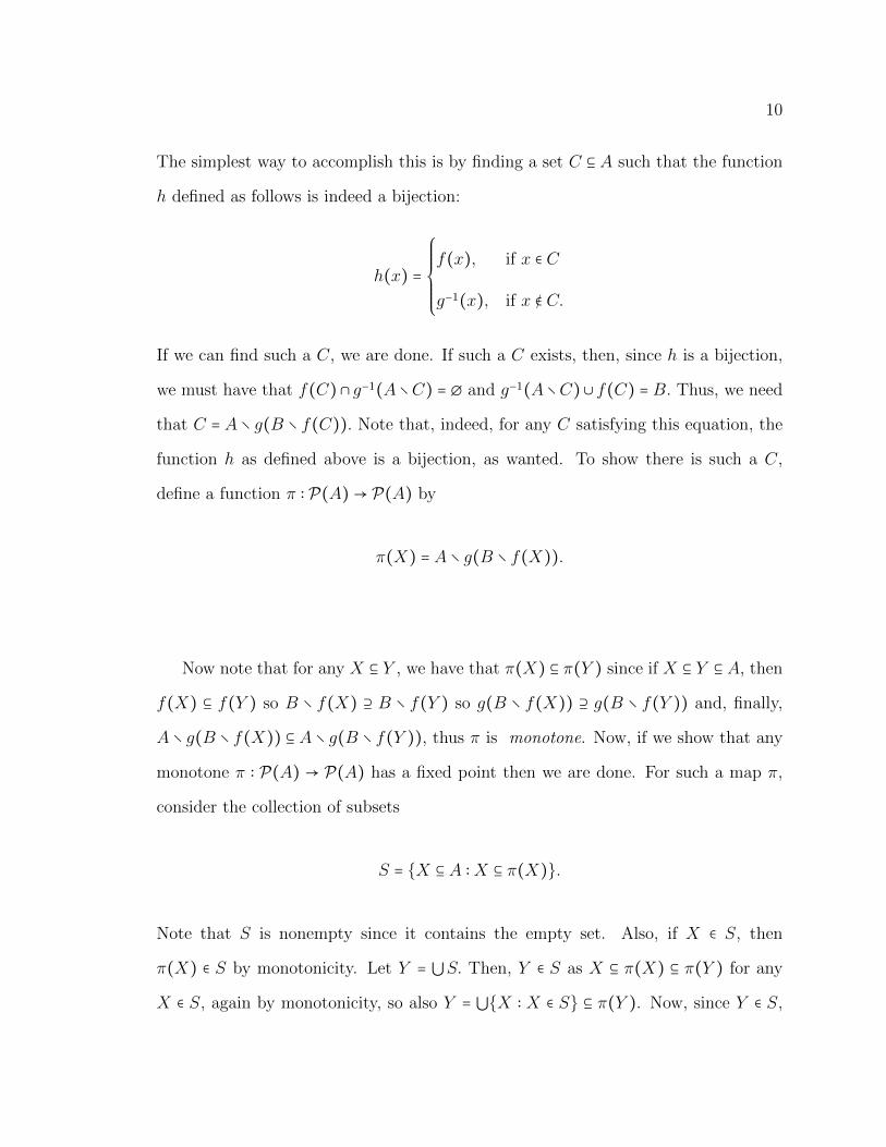
The simplest way to accomplish this is by finding a set C ⊆ A such that the function
h defined as follows is indeed a bijection:
h(x) =
⎧⎪⎪⎪⎪⎪⎨⎪⎪⎪⎪⎪⎩
f(x), if x ∈ C
g−1(x), if x ∉ C.
If we can find such a C, we are done. If such a C exists, then, since h is a bijection,
we must have that f(C)∩ g−1(A∖C) = ∅ and g−1(A∖C)∪ f(C) = B. Thus, we need
that C = A ∖ g(B ∖ f(C)). Note that, indeed, for any C satisfying this equation, the
function h as defined above is a bijection, as wanted. To show there is such a C,
define a function π ∶ P(A)→ P(A) by
π(X) = A ∖ g(B ∖ f(X)).
Now note that for any X ⊆ Y , we have that π(X) ⊆ π(Y ) since if X ⊆ Y ⊆ A, then
f(X) ⊆ f(Y ) so B ∖ f(X) ⊇ B ∖ f(Y ) so g(B ∖ f(X)) ⊇ g(B ∖ f(Y )) and, finally,
A ∖ g(B ∖ f(X)) ⊆ A ∖ g(B ∖ f(Y )), thus π is monotone. Now, if we show that any
monotone π ∶ P(A) → P(A) has a fixed point then we are done. For such a map π,
consider the collection of subsets
S = {X ⊆ A ∶X ⊆ π(X)}.
Note that S is nonempty since it contains the empty set. Also, if X ∈ S, then
π(X) ∈ S by monotonicity. Let Y = ⋃S. Then, Y ∈ S as X ⊆ π(X) ⊆ π(Y ) for any
X ∈ S, again by monotonicity, so also Y = ⋃{X ∶ X ∈ S} ⊆ π(Y ). Now, since Y ∈ S,
11
A B
C f(C)
g(B ∖ f(C)) B ∖ f(C)
f
g
Figure 1.1: The desired mapping
then also π(Y ) ∈ S, thus π(Y ) ⊆ ⋃S = Y. This means that Y = π(Y ), thus Y is a
fixed point.
Note that up to this point, we have not invoked the axiom of choice. Had we done
so, the proof of Theorem 1.13 would have been far less involved.
Definition 1.14. Let A be a set. If there is a function f ∶ A→ N that is injective, we
say that A is countable. If there is such an f that is bijective, we say A is countably
infinite.
Proposition 1.15. Any subset of a countable set is countable.
Proof. Let A be a countable set, as witnessed by f . Consider B ⊆ A. Clearly f ↾B is
also injective. Thus, B is countable.
12
Lemma 1.16. A set A is countable and nonempty if and only if there exists a
surjection f ′ ∶ N→ A.
Proof. Suppose A is countable and nonempty, so there exists some f ∶ A→ N injective.
Letting B = f(A), we have that f ∶ A → B is a bijection. Fix a ∈ A and define
f ′ ∶ N→ A by
f ′(n) =
⎧⎪⎪⎪⎪⎪⎨⎪⎪⎪⎪⎪⎩
f−1(n) if n ∈ B
a if n ∉ B
Then, f ′ is surjective. Conversely, if f ′ ∶ N → A is surjective, then A is nonempty.
Define f ∶ A → N as follows: Given a ∈ A, let f(a) be the least n ∈ N such that
f ′(n) = a, which exists since f ′ is surjective. Then, f is injective and, by definition,
A is countable.
Proposition 1.17. A ∪B is countable if and only if A and B are countable.
Proof. If A ∪B is countable, by Proposition 1.15, A and B are countable since they
are subsets of a countable set. Now suppose A and B are countable. If A = ∅, then
A ∪B = B, and similarly if B = ∅, so we may assume that A and B are nonempty.
By Lemma 1.16, there exist surjections f ′ ∶ N → A and g′ ∶ N → B. Let C = A ∪B.
Define h ∶ N→ C by
h(2x + 1) = f ′(x)
and
h(2x) = g′(x),
for x ∈ N. Clearly, h is surjective. By Lemma 1.16, it follows that C is countable.
Corollary 1.18. A finite union of countable sets is countable.
13
Proof. Immediate from Proposition 1.17 and induction.
Lemma 1.19. The Cartesian Product N ×N is countable.
Proof. Define
f ∶ N ×N→ N
by
f(m,n) = 2m3n.
By unique factorization, it is clear that f is injective and therefore N×N is countable.
Remark 1.20. Since N injects into N×N, it follows that N×N and N are equipotent,
by Theorem 1.13. Actually, it is possible to exhibit a bijection between the two sets
without using Theorem 1.13. For example, we can take
f ∶ N ×N→ N
to be
f(n,m) = 2n(2m + 1) − 1,
or
(n +m + 1
2) +m.
Proposition 1.21. A countably infinite union of countable sets is countable.
Proof. Let Ai be countable for all i ∈ N. We may assume all Ai are nonempty. Let
fi ∶ N→ Ai be surjective for all i ∈ N. Now define
g ∶ N ×N→∞
⋃i=0
Ai
14
by
g(i,m) = fi(m), for all i,m ∈ N.
Now to see that g is surjective consider a ∈∞
⋃i=0
Ai. Then, a ∈ Aj for some j. Since
fj is surjective, there is an m ∈ N such that fj(m) = a, so g(j,m) = a and thus g
is surjective. Let g′ ∶ N → N × N be the inverse of an f as in Remark 1.20. Then,
g ○ g′ ∶ N→∞
⋃i=0
Ai is surjective and the result follows.
Remark 1.22. The argument above uses the axiom of choice, by simultaneously
picking a surjection fi ∶ N → Ai for each i. In many specific applications of Proposi-
tion 1.21, we can exhibit these surjections explicitly, and therefore avoid the need to
use the axiom of choice.
For A and B sets, let AB denote the set of functions from A to B and let ∣A∣∣B∣ be
its cardinality.
Corollary 1.23. Q is countable.
Proof. Q =∞
⋃n=1
{m/n ∣m ∈ Z}.
On the other hand, it is a well–known result of Cantor that R is uncountable. We
omit the argument.
Lemma 1.24. 2∣N∣ = ∣R∣.
Proof. It is well–known that the standard Cantor middle set C ⊆ R consists of all reals
of the form
x =∞
∑n=1
2an3n
where each an is 0 or 1. This gives us an obvious bijection between C and the set
{0,1}N. Hence,
2∣N∣ = ∣{0,1}N∣ = ∣C∣ ≤ ∣R∣.
15
Conversely, any real x is uniquely determined by Ax = {q ∈ Q ∣ q < x}, hence ∣R∣ ≤
∣P(Q)∣. But there is an obvious bijection (via characteristic functions) between P(Q)
and {0,1}Q. Since Q is countable, this set is in bijection with {0,1}N, and we have
∣R∣ ≤ 2∣N∣.
The result follows from the Schroder-Bernstein theorem.
Corollary 1.25. For any n ∈ Z+, if n > 1, then n∣N∣ = ∣R∣.
Proof. It suffices to prove that n∣N∣ ≤ 2∣N∣, by Lemma 1.24 and the Schroder-Bernstein
theorem. But note that n ≤ 2∣N∣, so n∣N∣ ≤ (2∣N∣)∣N∣. We claim that for any (nonempty)
sets A,B,C, we have
(∣A∣∣B∣)∣C∣ = ∣A∣∣B×C∣.
From this, it follows that (2∣N∣)∣N∣ = 2∣N∣, and we are done.
To prove the claim, we exhibit a bijection π between (AB)C and AB×C . Given
f ∶ C → AB, define π(f) ∶ B×C → A by π(f)(b, c) = (f(c))(b) for any b ∈ B and c ∈ C.
It is straightforward to check that π is indeed a bijection.
16
CHAPTER 2
THE CHROMATIC NUMBER OF THE PLANE
While the Four Color Theorem is by far the most celebrated result in Graph Coloring,
another result, if attained, would be heralded as equally important. The result in
question is the determination of the chromatic number of the plane, as yet unknown.
Definition 2.1. The chromatic number of the plane, denoted by χ, is the smallest
number of colors sufficient for coloring the plane in such a way that no two points of
the same color are unit distance apart.
Question 2.2. What is the value of χ?
Perhaps, it is the fact that this problem can be formulated in such an easy
to understand fashion that makes it so intriguing. However, the simplicity of this
question is merely the facade of an historically difficult problem. In fact, the best
known results say that χ is either 4, 5, 6, or 7. If a coloring of the plane is such that
no two points at distance 1 have the same color, we say it is a χ coloring. If a graph
cannot be colored such that no two points at distance 1 have the same color, we say
the graph cannot be χ colored.
Lemma 2.3. The Chromatic number of the plane is at least 3.
The following proof corresponds to Figure 2.1.
17
A
B C
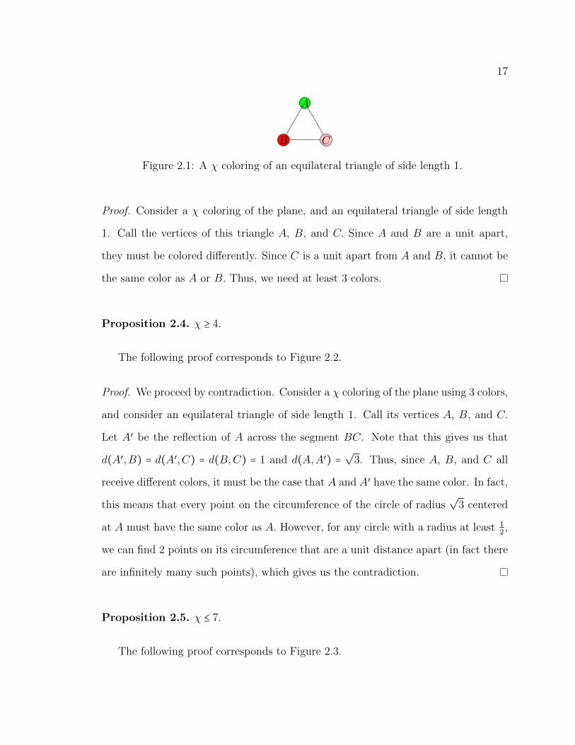
Figure 2.1: A χ coloring of an equilateral triangle of side length 1.
Proof. Consider a χ coloring of the plane, and an equilateral triangle of side length
1. Call the vertices of this triangle A, B, and C. Since A and B are a unit apart,
they must be colored differently. Since C is a unit apart from A and B, it cannot be
the same color as A or B. Thus, we need at least 3 colors.
Proposition 2.4. χ ≥ 4.
The following proof corresponds to Figure 2.2.
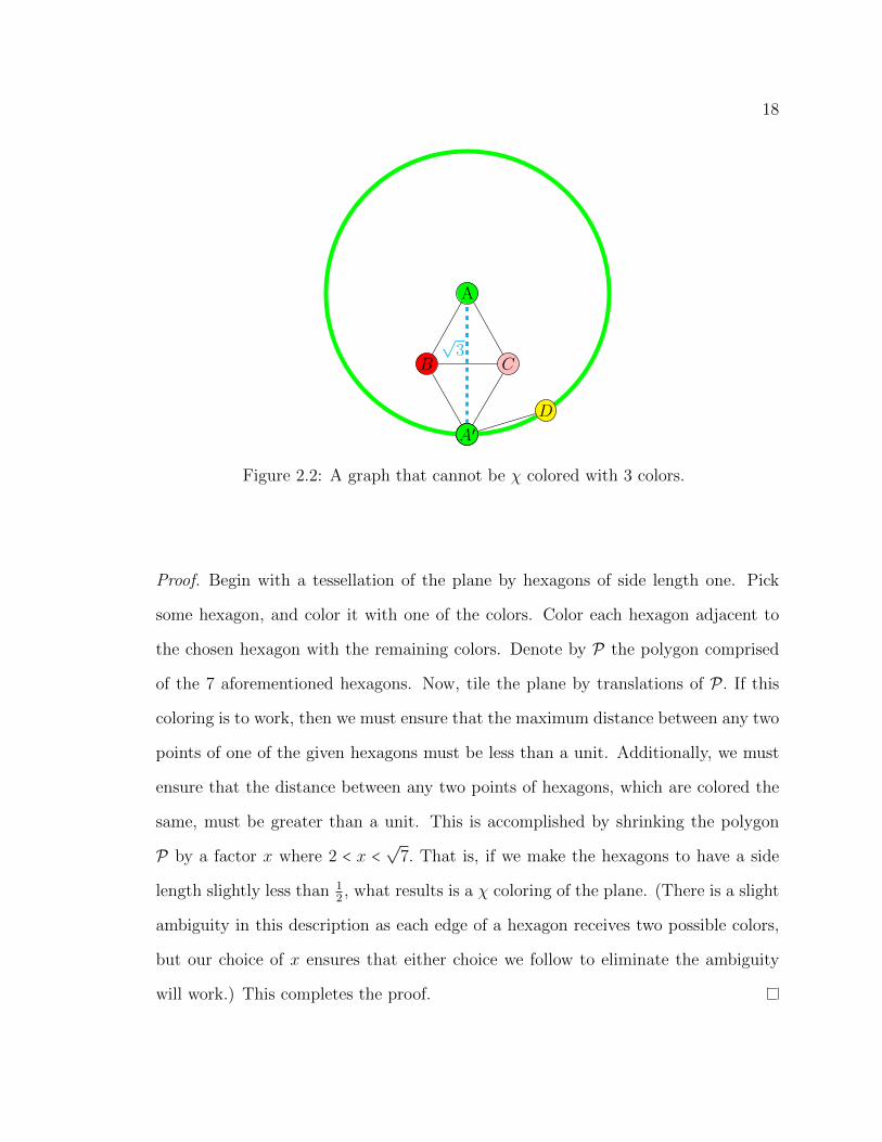
Proof. We proceed by contradiction. Consider a χ coloring of the plane using 3 colors,
and consider an equilateral triangle of side length 1. Call its vertices A, B, and C.
Let A′ be the reflection of A across the segment BC. Note that this gives us that
d(A′,B) = d(A′,C) = d(B,C) = 1 and d(A,A′) =√
3. Thus, since A, B, and C all
receive different colors, it must be the case that A and A′ have the same color. In fact,
this means that every point on the circumference of the circle of radius√
3 centered
at A must have the same color as A. However, for any circle with a radius at least 12 ,
we can find 2 points on its circumference that are a unit distance apart (in fact there
are infinitely many such points), which gives us the contradiction.
Proposition 2.5. χ ≤ 7.
The following proof corresponds to Figure 2.3.
18
A
B
√3
C
A′A′
D
Figure 2.2: A graph that cannot be χ colored with 3 colors.
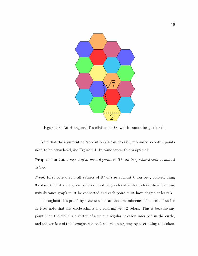
Proof. Begin with a tessellation of the plane by hexagons of side length one. Pick
some hexagon, and color it with one of the colors. Color each hexagon adjacent to
the chosen hexagon with the remaining colors. Denote by P the polygon comprised
of the 7 aforementioned hexagons. Now, tile the plane by translations of P. If this
coloring is to work, then we must ensure that the maximum distance between any two
points of one of the given hexagons must be less than a unit. Additionally, we must
ensure that the distance between any two points of hexagons, which are colored the
same, must be greater than a unit. This is accomplished by shrinking the polygon
P by a factor x where 2 < x <√
7. That is, if we make the hexagons to have a side
length slightly less than 12 , what results is a χ coloring of the plane. (There is a slight
ambiguity in this description as each edge of a hexagon receives two possible colors,
but our choice of x ensures that either choice we follow to eliminate the ambiguity
will work.) This completes the proof.
19
√7
2Figure 2.3: An Hexagonal Tessellation of R2, which cannot be χ colored.
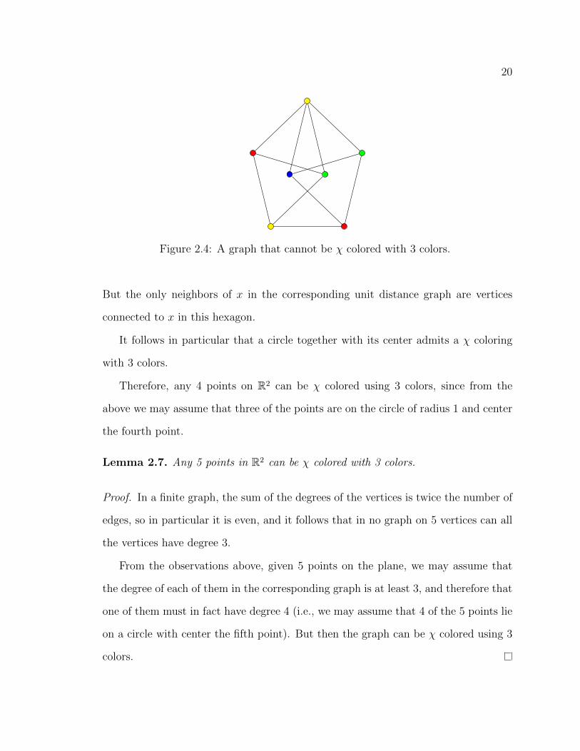
Note that the argument of Proposition 2.4 can be easily rephrased so only 7 points
need to be considered, see Figure 2.4. In some sense, this is optimal:
Proposition 2.6. Any set of at most 6 points in R2 can be χ colored with at most 3
colors.
Proof. First note that if all subsets of R2 of size at most k can be χ colored using
3 colors, then if k + 1 given points cannot be χ colored with 3 colors, their resulting
unit distance graph must be connected and each point must have degree at least 3.
Throughout this proof, by a circle we mean the circumference of a circle of radius
1. Now note that any circle admits a χ coloring with 2 colors. This is because any
point x on the circle is a vertex of a unique regular hexagon inscribed in the circle,
and the vertices of this hexagon can be 2-colored in a χ way by alternating the colors.
20
Figure 2.4: A graph that cannot be χ colored with 3 colors.
But the only neighbors of x in the corresponding unit distance graph are vertices
connected to x in this hexagon.
It follows in particular that a circle together with its center admits a χ coloring
with 3 colors.
Therefore, any 4 points on R2 can be χ colored using 3 colors, since from the
above we may assume that three of the points are on the circle of radius 1 and center
the fourth point.
Lemma 2.7. Any 5 points in R2 can be χ colored with 3 colors.
Proof. In a finite graph, the sum of the degrees of the vertices is twice the number of
edges, so in particular it is even, and it follows that in no graph on 5 vertices can all
the vertices have degree 3.
From the observations above, given 5 points on the plane, we may assume that
the degree of each of them in the corresponding graph is at least 3, and therefore that
one of them must in fact have degree 4 (i.e., we may assume that 4 of the 5 points lie
on a circle with center the fifth point). But then the graph can be χ colored using 3
colors.
21
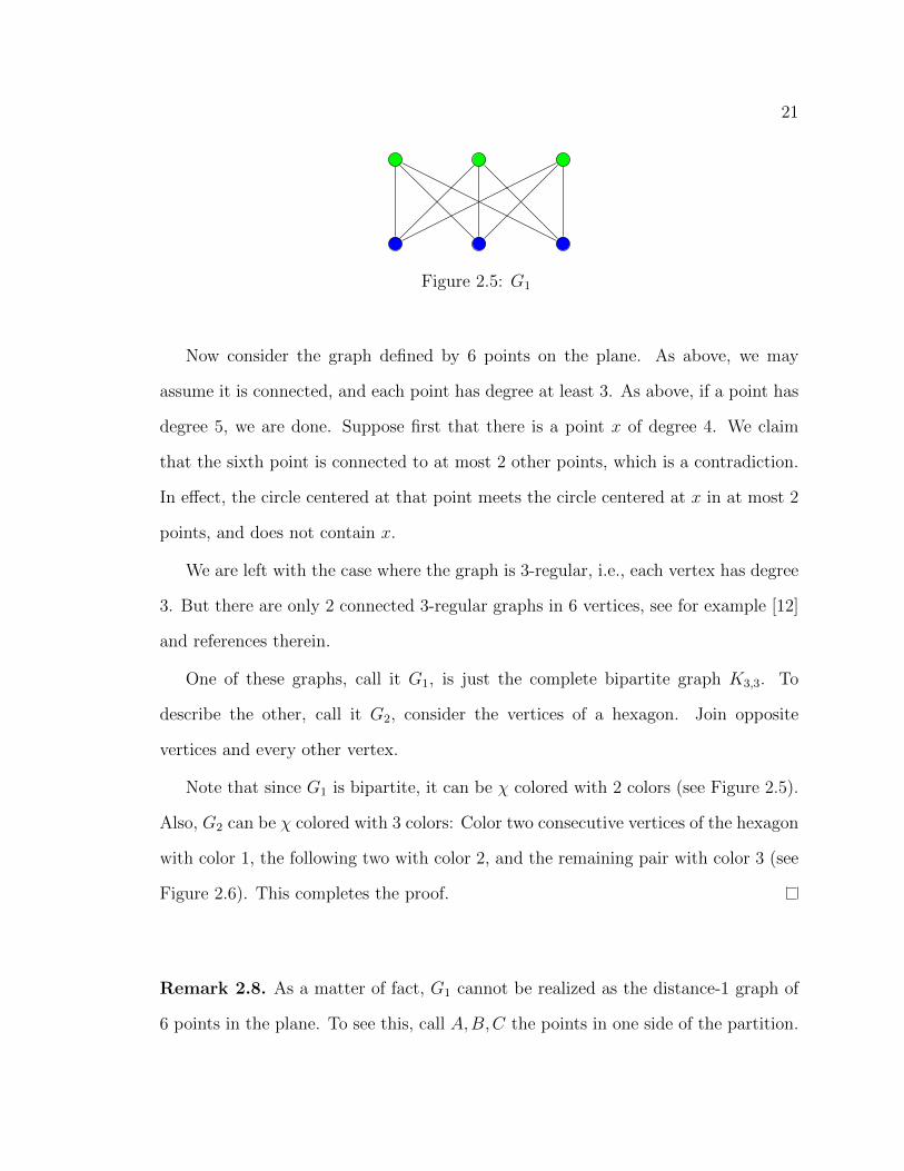
Figure 2.5: G1
Now consider the graph defined by 6 points on the plane. As above, we may
assume it is connected, and each point has degree at least 3. As above, if a point has
degree 5, we are done. Suppose first that there is a point x of degree 4. We claim
that the sixth point is connected to at most 2 other points, which is a contradiction.
In effect, the circle centered at that point meets the circle centered at x in at most 2
points, and does not contain x.
We are left with the case where the graph is 3-regular, i.e., each vertex has degree
3. But there are only 2 connected 3-regular graphs in 6 vertices, see for example [12]
and references therein.
One of these graphs, call it G1, is just the complete bipartite graph K3,3. To
describe the other, call it G2, consider the vertices of a hexagon. Join opposite
vertices and every other vertex.
Note that since G1 is bipartite, it can be χ colored with 2 colors (see Figure 2.5).
Also, G2 can be χ colored with 3 colors: Color two consecutive vertices of the hexagon
with color 1, the following two with color 2, and the remaining pair with color 3 (see
Figure 2.6). This completes the proof.
Remark 2.8. As a matter of fact, G1 cannot be realized as the distance-1 graph of
6 points in the plane. To see this, call A,B,C the points in one side of the partition.
22
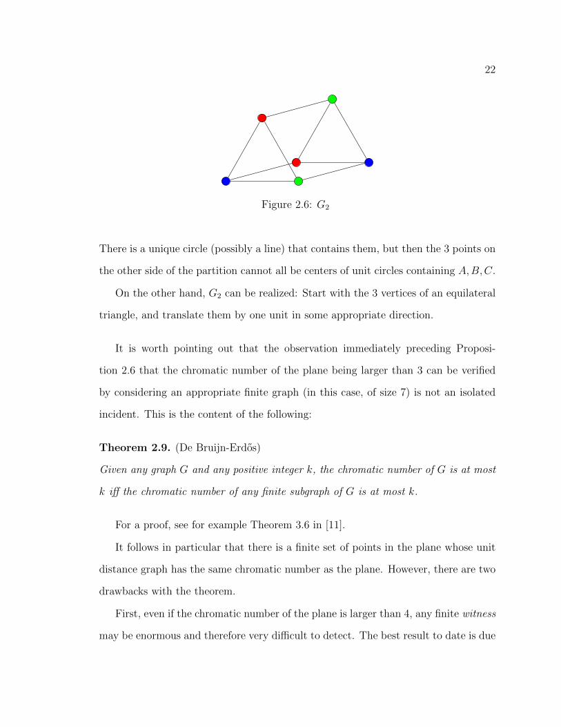
Figure 2.6: G2
There is a unique circle (possibly a line) that contains them, but then the 3 points on
the other side of the partition cannot all be centers of unit circles containing A,B,C.
On the other hand, G2 can be realized: Start with the 3 vertices of an equilateral
triangle, and translate them by one unit in some appropriate direction.
It is worth pointing out that the observation immediately preceding Proposi-
tion 2.6 that the chromatic number of the plane being larger than 3 can be verified
by considering an appropriate finite graph (in this case, of size 7) is not an isolated
incident. This is the content of the following:
Theorem 2.9. (De Bruijn-Erdos)
Given any graph G and any positive integer k, the chromatic number of G is at most
k iff the chromatic number of any finite subgraph of G is at most k.
For a proof, see for example Theorem 3.6 in [11].
It follows in particular that there is a finite set of points in the plane whose unit
distance graph has the same chromatic number as the plane. However, there are two
drawbacks with the theorem.
First, even if the chromatic number of the plane is larger than 4, any finite witness
may be enormous and therefore very difficult to detect. The best result to date is due
23
to Dan Pritkin in [14], where it is shown that the distance-1 graph of any 12 points
in R2 is 4-colorable.
Second, the proof of the De Bruijn-Erdos Theorem is strictly non-constructive, as
it uses in an essential way the axiom of choice, in the form of the compactness of an
appropriate product of (Hausdorff) compact spaces. Given our current knowledge, it
is not unconceivable that there are models of set theory where the axiom of choice
fails, every finite subset of the plane has chromatic number at most 4, and the plane
itself a has larger chromatic number. These matters are discussed in detail in [4].
The situation above is not entirely hypothetical. For example, it is shown in [13]
that if we restrict our attention to Lebesgue measurable colorings, then the chromatic
number of the plane is at least 5. See also [4].
24
CHAPTER 3
REGRESSIVE FUNCTIONS ON PAIRS
This short chapter builds on Caicedo [9]. It concerns the following coloring problem:
For m ≤ l positive integers, consider the complete graph G = G(m, l) on the set
of vertices V = {m,m + 1, . . . , l}. A regressive coloring of G is a function that assigns
to each edge {a, b} of G a color c, that is a natural number strictly less than both
a and b: 0 ≤ c < min{a, b}. These colorings are natural to consider in the context of
canonical Ramsey theory.
Given a coloring f of G, a min-homogeneous set is a subset H of V such that
whenever a < b < c are in H, then f({a, b}) = f({a, c}), i.e., whenever d is an edge
with vertices in H, f(d) only depends on the minimum of d. We say that H is
homogeneous if f is constant on edges from H.
Typically, in Ramsey theory, one proves that a coloring of a large graph admits
appropriately sized homogeneous sets. This is not possible in general in this context:
Simply consider the coloring f(d) = min(d) − 1.
On the other hand, as shown in Section 3 of [9], for any m and n there is an l such
that any regressive coloring of G(m, l) admits a min-homogeneous set of at least n
elements.
Denote by g(n,m) the smallest possible l such that the above holds. The following
values of g are established in [9]:
25
1. g(4,2) = 15.
2. g(4,3) = 37.
3. g(4,4) ≤ 85.
We now give the following result.
Theorem 3.1. g(4,4) = 85.
Proof. This follows by constructing a regressive coloring f of G(4,84) which contains
no min-homogeneous set of size 4. The function was constructed and verified using
Matlab, modifying a coloring from [9] that proves the weaker bound g(4) ≥ 2g(3)+3 =
77. Its definition, and the code that verifies it works, can be found in Appendix
A.1.
Let us remark that the arguments of [9] give in general that
g(4, n) ≤ 2nn + 12 ⋅ 2n−3 + 1
for n ≥ 3. We close the chapter by stating without proof an improvement:
Fact 3.2. (Caicedo)
For all positive n, we have that g(4, n) ≤ 2n−1(n + 7) − 3.
26
CHAPTER 4
SATISFACTORY COLORINGS
4.1 The Problem
Question 4.1. Is it possible to color the positive integers using n colors, in such a
way that for any a, the numbers a,2a,3a, ..., na receive different colors?
We call satisfactory a coloring witnessing a positive answer to Question 4.1.
Question 4.1 was posted by Palvolgyi Domotor to MathOverflow.net [2], a website
whose stated primary goal is for users to ask and answer research level mathematics
questions. The question, as Domotor states in his post, is an extension of a problem
originally published in the Hungarian journal KoMaL (Kozepiskolai Matematikai es
Fizikai Lapok), a Mathematics and Physics journal primarily aimed at High School
Students. In the April, 2010 issue, problem A.506 asked to show that there is a
satisfactory coloring whenever n + 1 is prime [3]. In full generality, Question 4.1
remains open.
In addition to asking the question of whether there are satisfactory colorings for
a given n, it is natural to ask the following:
Question 4.2. Given n, how many satisfactory colorings for n are there, if any at
all?
27
We start by discussing an example. Then, we use the insight gained there to
answer Question 4.2. We begin approaching Question 4.1 in the next chapter.
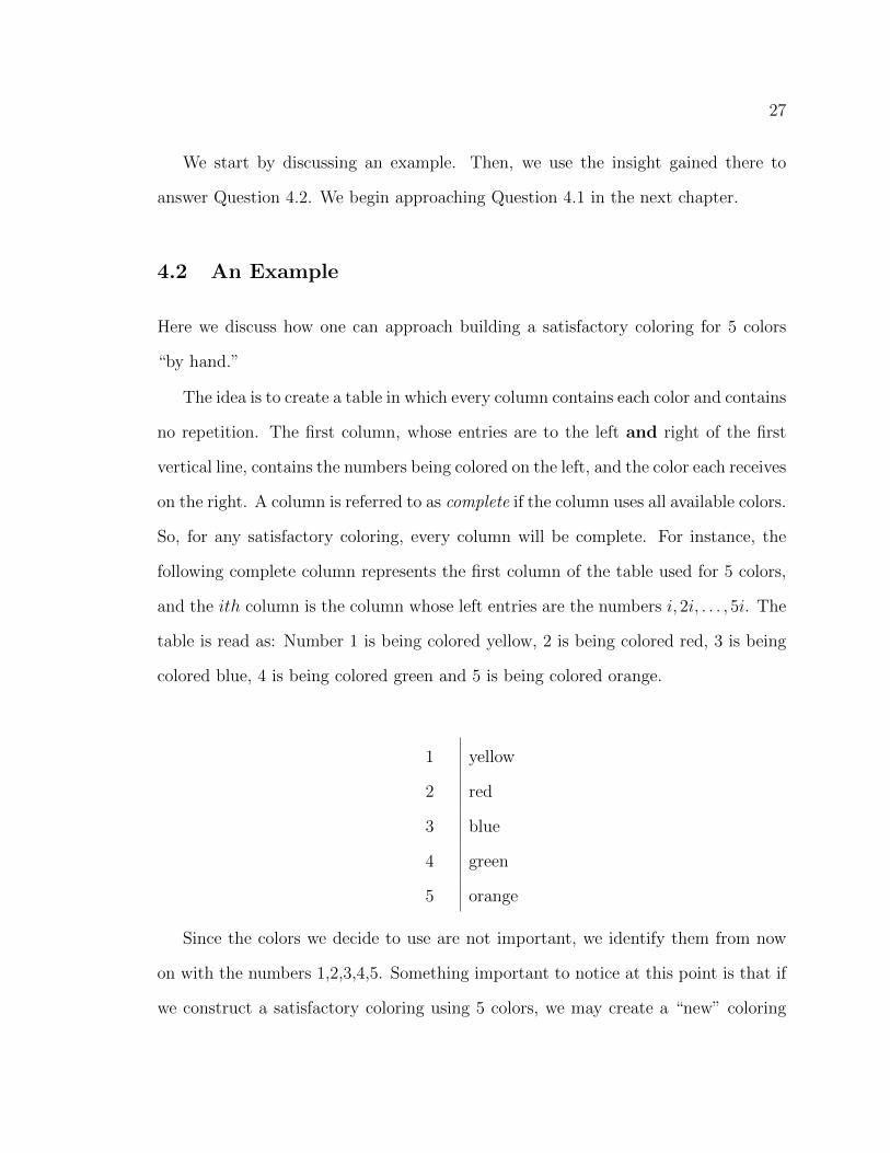
4.2 An Example
Here we discuss how one can approach building a satisfactory coloring for 5 colors
“by hand.”
The idea is to create a table in which every column contains each color and contains
no repetition. The first column, whose entries are to the left and right of the first
vertical line, contains the numbers being colored on the left, and the color each receives
on the right. A column is referred to as complete if the column uses all available colors.
So, for any satisfactory coloring, every column will be complete. For instance, the
following complete column represents the first column of the table used for 5 colors,
and the ith column is the column whose left entries are the numbers i,2i, . . . ,5i. The
table is read as: Number 1 is being colored yellow, 2 is being colored red, 3 is being
colored blue, 4 is being colored green and 5 is being colored orange.
1 yellow
2 red
3 blue
4 green
5 orange
Since the colors we decide to use are not important, we identify them from now
on with the numbers 1,2,3,4,5. Something important to notice at this point is that if
we construct a satisfactory coloring using 5 colors, we may create a “new” coloring
28
by simply permuting the colors. This means that for every satisfactory coloring
there are precisely 5! ways in which the colors can be assigned for the first column.
However, this “new” coloring is merely a permutation of the original coloring and,
thus, offers no additional information and we regard any two colorings obtained this
way as identical.
Suppose that c is a satisfactory coloring using 5 colors,
c ∶ Z+ → {1,2,3,4,5}.
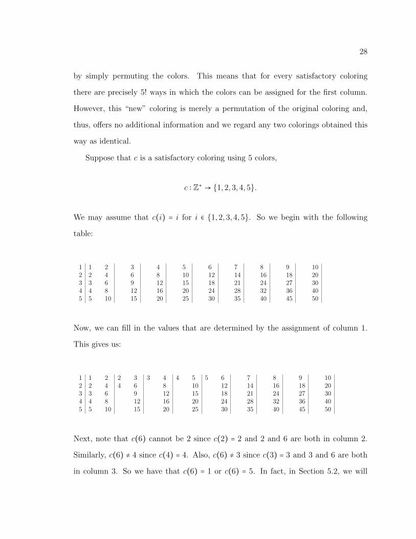
We may assume that c(i) = i for i ∈ {1,2,3,4,5}. So we begin with the following
table:
1 1 2 3 4 5 6 7 8 9 102 2 4 6 8 10 12 14 16 18 203 3 6 9 12 15 18 21 24 27 304 4 8 12 16 20 24 28 32 36 405 5 10 15 20 25 30 35 40 45 50
Now, we can fill in the values that are determined by the assignment of column 1.
This gives us:
1 1 2 2 3 3 4 4 5 5 6 7 8 9 102 2 4 4 6 8 10 12 14 16 18 203 3 6 9 12 15 18 21 24 27 304 4 8 12 16 20 24 28 32 36 405 5 10 15 20 25 30 35 40 45 50
Next, note that c(6) cannot be 2 since c(2) = 2 and 2 and 6 are both in column 2.
Similarly, c(6) ≠ 4 since c(4) = 4. Also, c(6) ≠ 3 since c(3) = 3 and 3 and 6 are both
in column 3. So we have that c(6) = 1 or c(6) = 5. In fact, in Section 5.2, we will
29
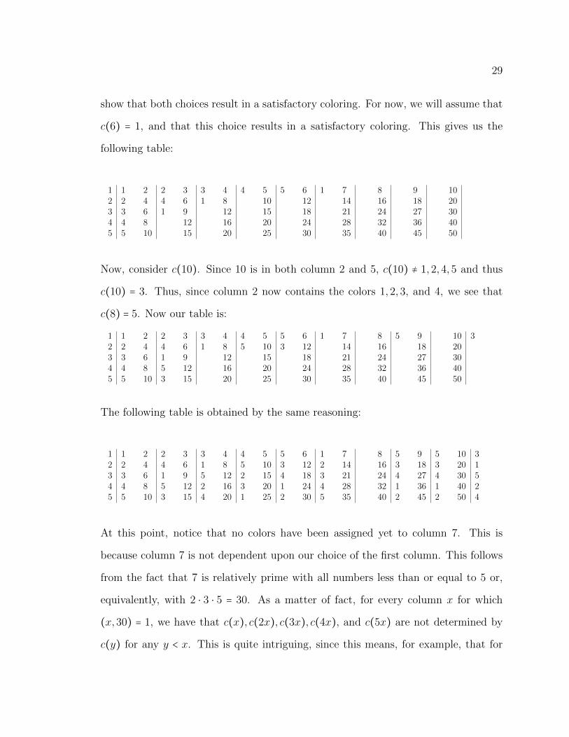
show that both choices result in a satisfactory coloring. For now, we will assume that
c(6) = 1, and that this choice results in a satisfactory coloring. This gives us the
following table:
1 1 2 2 3 3 4 4 5 5 6 1 7 8 9 102 2 4 4 6 1 8 10 12 14 16 18 203 3 6 1 9 12 15 18 21 24 27 304 4 8 12 16 20 24 28 32 36 405 5 10 15 20 25 30 35 40 45 50
Now, consider c(10). Since 10 is in both column 2 and 5, c(10) ≠ 1,2,4,5 and thus
c(10) = 3. Thus, since column 2 now contains the colors 1,2,3, and 4, we see that
c(8) = 5. Now our table is:
1 1 2 2 3 3 4 4 5 5 6 1 7 8 5 9 10 32 2 4 4 6 1 8 5 10 3 12 14 16 18 203 3 6 1 9 12 15 18 21 24 27 304 4 8 5 12 16 20 24 28 32 36 405 5 10 3 15 20 25 30 35 40 45 50
The following table is obtained by the same reasoning:
1 1 2 2 3 3 4 4 5 5 6 1 7 8 5 9 5 10 32 2 4 4 6 1 8 5 10 3 12 2 14 16 3 18 3 20 13 3 6 1 9 5 12 2 15 4 18 3 21 24 4 27 4 30 54 4 8 5 12 2 16 3 20 1 24 4 28 32 1 36 1 40 25 5 10 3 15 4 20 1 25 2 30 5 35 40 2 45 2 50 4
At this point, notice that no colors have been assigned yet to column 7. This is
because column 7 is not dependent upon our choice of the first column. This follows
from the fact that 7 is relatively prime with all numbers less than or equal to 5 or,
equivalently, with 2 ⋅ 3 ⋅ 5 = 30. As a matter of fact, for every column x for which
(x,30) = 1, we have that c(x), c(2x), c(3x), c(4x), and c(5x) are not determined by
c(y) for any y < x. This is quite intriguing, since this means, for example, that for
30
every prime we encounter greater than 5 we will, in some sense, be starting from the
beginning. By this, we mean that for every integer x > 5 with (x,30) = 1, there will
be 5! ways in which we can color column x that will result in a satisfactory coloring.
This observation leads us to the key notion of the n-core, and to the following results,
the first of which deals with extending a coloring of the core to all positive integers
and the second, a corollary of the first, identifies the number of satisfactory colorings
there are in the case of n colors, provided a coloring of the core does in fact exist.
4.3 The Core
Definition 4.3. The n-core, or simply the core if n is understood, is the set K =Kn
of all positive integers whose prime decomposition only involves primes less than or
equal to n.
Definition 4.4. Say that X ⊆ Z+ is n-appropriate iff X is nonempty and contains
ai and a/j whenever a ∈X, i, j ≤ n, and j divides a.
If X is n-appropriate, say that c ∶ X → {1, . . . , n} is satisfactory iff c(ai) ≠ c(aj)
whenever a ∈X and i < j ≤ n. Note that this notion coincides with the previous notion
of satisfactory when X = Z+.
We denote by An the set of numbers relatively prime to n!, i.e., those positive
integers whose prime decomposition only involves prime numbers strictly larger than
n.
If X ⊆ Z+ and k ∈ Z+, we denote by k ⋅X the dilation of X by factor k:
k ⋅X = {ka ∶ a ∈X}.
31
The notation X = ⊍a∈BXa means both that X is the union of the Xa for a ∈ B, and
that the sets Xa are pairwise disjoint.
Lemma 4.5. A set X ⊆ Z+ is n-appropriate iff there is a nonempty set B ⊆ An such
that
X = ⊍k∈B
k ⋅Kn.
Moreover, if this is the case, then we have B = An ∩X.
Proof. Note that Kn is n-appropriate and therefore so is k ⋅Kn for any k ∈ An. It
follows that any X of the form ⊍k∈B k ⋅Kn for B ⊆ An and nonempty is n-appropriate
as well.
Towards the converse, suppose now that X is n-appropriate. From the uniqueness
of prime factorization, it follows that each m ∈ Z+ can be uniquely written in the
form m = kmbm where km ∈ An and bm ∈ Kn. Let B = {km ∶ m ∈ X}. We claim that
X = ⊍k∈B k ⋅Kn.
First, note that if x ≠ y are in An, then x ⋅Kn and y ⋅Kn are pairwise disjoint.
Now, if k ∈ B, then there is some m ∈ X such that k = km. By assumption, h/j ∈ X
whenever h ∈ X and j ≤ n divides h. It follows immediately that in fact h/j ∈ X
whenever h ∈X and j ∈Kn divides h. In particular, k = km =m/bm ∈X. Similarly, by
assumption hi ∈ X whenever h ∈ Xand i ≤ n, and it follows immediately that hi ∈ X
whenever h ∈X and i ∈Kn. Therefore, k ⋅Kn ⊆X. This means that
⋃k∈B
k ⋅Kn ⊆X.
But, if m ∈X, then m ∈ km ⋅Kn, and we have that
32
⋃k∈B
k ⋅Kn ⊇X.
This proves the equality, and since (as addressed above) the union is disjoint, this
completes the proof.
Note that we have shown that if X is n-appropriate and B is as above, then in fact
B = An ∩X. Since the sets k ⋅Kn are pairwise disjoint as k varies over Kn, it follows
that for any n-appropriate X there is a unique B ⊆ An such that X = ⋃k∈B k ⋅Kn, and
we are done.
For X n-appropriate, let
CX = {c ∶X → {1, . . . , n} ∶ c is satisfactory},
and denote by C the set CZ+ .
The following theorem shows that C ≠ ∅ iff CX ≠ ∅ for some n-appropriate set X
iff CX ≠ ∅ for all n-appropriate sets X.
In particular, it follows that the question of whether there are any satisfactory
colorings for n is really a question about whether there are satisfactory colorings of
the n-core Kn. In fact, the theorem shows how the satisfactory colorings of the core
completely determine all satisfactory colorings.
Theorem 4.6. 1. Suppose X ⊆ Y are n-appropriate. If CY ≠ ∅, then CX ≠ ∅. In
fact, c ↾X ∈ CX for any c ∈ CY .
2. Given k ∈ An, if c ∈ Ck⋅Kn, let c′ ∶ Kn → {1, . . . , n} be the map given by c′(b) =
c(kb). Then, c′ ∈ CKn.
33
3. Given k ∈ An, if c ∈ CKn, let ck ∶ k ⋅ Kn → {1, . . . , n} be the map given by
ck(m) = c(m/k). Then, ck ∈ Ck⋅Kn.
4. Suppose that CKn ≠ ∅ and X is n-appropriate. Then, c ∈ CX iff for each
k ∈ An ∩X, there is a map ck ∈ CKn such that
c = ⋃k∈An∩X
ckk.
5. C ≠ ∅ iff CX ≠ ∅ for any n-appropriate X iff CX ≠ ∅ for some n-appropriate
set X. Moreover if X ⊆ Y are n-appropriate, then d ∈ CX iff d = c ↾X for some
c ∈ CY .
Proof. (1) This is clear.
(2) Given k ∈ An and c ∈ Ck⋅Kn , if c′ is defined as in item 2, then c′(ib) = c(kib) ≠
c(kjb) = c′(jb) for any b ∈ Kn and i < j ≤ n since c is satisfactory. But, then c′ is
satisfactory as well.
(3) Conversely, if c ∈ CKn , k ∈ An, and ck is defined as in item 3, then ck(im) =
c(i(m/k)) ≠ c(j(m/k)) = ck(jm) for any m ∈ k ⋅Kn and i < j ≤ n since c is satisfactory.
But, then ck is satisfactory as well.
(4) Suppose that CKn ≠ ∅ and X is n-appropriate. For each k ∈ An∩X let ck ∈ CKn
and define c = ⋃k∈An∩X ckk. As shown in Lemma 4.5, k ⋅Kn ∩ l ⋅Kn = ∅ whenever k ≠ l
are in An. From this, and item 3, c is well defined and has domain ⋃k∈An∩X k ⋅Kn,
which equals X, again by Lemma 4.5. Suppose m ∈ X and i < j ≤ n. Then, there is
a unique k ∈ An ∩X such that mi and mj belong to k ⋅Kn, and by item 3 it follows
that c(mi) ≠ c(mj). This proves that c is satisfactory.
34
Conversely, if c ∈ CX , then d = c ↾ k ⋅Kn ∈ Ck⋅Kn for any k ∈ An ∩X, by item 1,
and ck = d′ ∈ CKn by item 2. But d = d′k, i.e., c = ⋃k∈An∩X ckk, and this completes the
proof of item 4.
(5) Now, if X is n-appropriate, and CX ≠ ∅, then Ck⋅Kn ≠ ∅ for any k in the
nonempty set An ∩X, by item 1. But then CKn ≠ ∅, by item 2. It follows from item
4 that C = CZ+ ≠ ∅. But then CY ≠ ∅ for any n-appropriate Y , again by item 1.
Finally, if X ⊆ Y are n-appropriate and c ∈ CY , then d = c ↾ X ∈ CX , by item
1. Conversely, if d ∈ CX , let e ∈ CKn , which exists as shown above. Let ck = e for
k ∈ An ∩ (Y ∖X). For k ∈ An ∩X, let ck = (d ↾ k ⋅Kn)′. As in item 4, we have that
c = ⋃k∈An∩Y ckk ∈ CY . And, by construction, d = c ↾ X. This completes the proof of
item 5.
The importance of this theorem is paramount. It provides us with the ability to
restrict our attention from all of Z+ to a set comprised of elements with an inherent
underlying structure. As such, it has played a dominant role in many of our results.
The relation between arbitrary satisfactory colorings and colorings of the core
detailed in Theorem 4.6 has the following corollary:
Corollary 4.7. For n > 1, with C and CKn as above, if CKn ≠ ∅ then ∣C ∣ = ∣R∣ .
Proof. As explained in Section 4.2, if there is a coloring of the core, there are at
least n! ≥ 2 such colorings (obtained by simply permuting the colors). Note that An
is countably infinite. By item 4 of Theorem 4.6, there is a bijective correspondence
between the elements of C, and the set of functions from An to CKn : ∣C ∣ = ∣CAn
Kn∣ ≥
n!∣An∣ = ∣R∣, by Corollary 1.25.
On the other hand, any element of C is a function from Z+ to {1, . . . , n}, so
∣C ∣ ≤ ∣{1, . . . , n}Z+ ∣ = n∣N∣ = ∣R∣, by Corollary 1.25.
35
It follows that ∣C ∣ = ∣R∣, by the Schroder-Bernstein theorem.
Convention 4.8. Note that we may further require that if c ∈ C, then c(i) = i
for i ≤ n, without affecting the above computations, and we assume this further
requirement from now on.
What Theorem 4.6 and Corollary 4.7 give us can be interpreted as follows. If
there is a satisfactory coloring of Kn, then there are continuum many satisfactory
colorings of Z+ using n colors. However, this abundance of colorings is a distraction
since the underlying structure of any satisfactory coloring can be described in terms
of what is happening on the core.
36
CHAPTER 5
STRONG REPRESENTATIONS
5.1 Strong Representatives
In this section, we present a condition on n ensuring the existence of satisfactory
colorings with n colors. The construction below was suggested in MathOverflow by
Victor Protsak, see [2].
From now on, we denote by n the set {1,2, . . . , n}.
Theorem 5.1. Let n, k ∈ N. If p = nk + 1 is prime, and 1k,2k,3k, . . . , nk are distinct
modulo p, then the following produces a satisfactory coloring: Let
ϕ ∶ {ik (mod p) ∶ i ∈ n}→ n
be the bijection given by ϕ(ik (mod p)) = i. Given m ∈ Z+, write it as m = apr where
(a, p) = 1 and r ∈ N. Now define c(m) = ϕ(ak (mod p)).
Proof. We begin noting that by Corollary 1.7 there are exactly n pairwise incongruent
nonzero kth power residues modulo nk + 1. It follows that, for any b with (b, p) = 1,
bk = jk (mod p) for some j ∈ n. Now let d, e ∈ n. We need to argue that c(dm) =
c(em) if and only if d = e. To see this, consider dm = adpr. Thus, c(dm) = ϕ((ad)k
(mod p)). Similarly, we have that c(em) = ϕ((ae)k (mod p)). Since ϕ is a bijection,
37
c(dm) = c(em) implies that (ad)k ≡ (ae)k (mod p) and therefore dk ≡ ek (mod p), so
d = e by assumption.
This leads us to the following definition.
Definition 5.2. Strong Representations.
A satisfactory coloring c ∶Kn → n admits a strong representation if and only if there
exists a prime p of the form nk + 1 such that 1k, . . . , nk are pairwise distinct modulo
p and, letting
ϕ ∶ n→ {ak (mod p) ∶ a ∈ n}
be the map
ϕ(i) = ik (mod p),
then
ϕ ○ c(a) = ak (mod p)
for all a. In this case, we call ϕ the strong representation of c, and p the associated
prime. We also say that p is a strong representative of order n (for c).
Theorem 5.1 lends us the ability to construct a satisfactory coloring in a very
simple way. However, granting the existence of such a prime has eluded us. In fact,
at this time, we have only found nontrivial strong representatives of order 32 or less.
Here, a prime of the form p = nk+1 is nontrivial iff k > 2. We call these primes trivial
when k ≤ 2, since the requirement of Theorem 5.1 is automatically satisfied in this
case, see Subsection 5.1.1.
As evidence of how incredibly difficult the search for strong representatives is,
we mention the following. The smallest strong representative of order 32 is p =
38
5,209,690,063,553. Identifying it took nearly one month of cpu time on an Intel
CoreTMi7 machine.
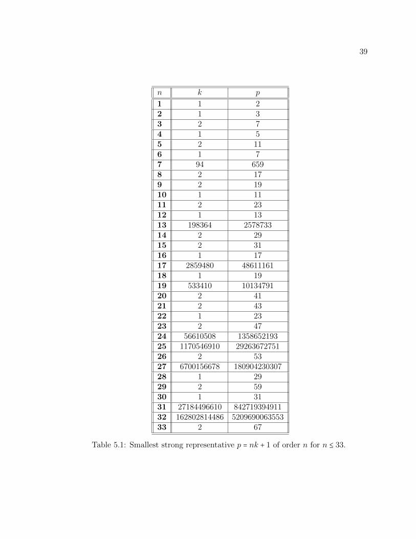
Table 5.1 lists for n ≤ 33 the smallest strong representative p = nk + 1 of order n.
5.1.1 Trivial Representatives
It is clear from Theorem 5.1 that if p = n + 1 is prime, then the coloring
c(m) = a (mod p)
where m = apr, (a, p) = 1, is a satisfactory coloring with n colors. This solves the
question originally asked in KoMal [3] . From the infinitude of the primes, we have:
Corollary 5.3. There are infinitely many values of n for which a satisfactory coloring
exists.
An easy observation also gives us:
Theorem 5.4. If p = 2n + 1 is prime, then the map
c(m) = a2 (mod p)
where m = apr, (a, p) = 1, induces a satisfactory coloring with n colors.
Proof. We must show that if 1 ≤ i < j ≤ n, then i2 /≡ j2 (mod p), as the result then
follows from Theorem 5.1. But, i2 ≡ j2 (mod p) implies that p∣j − i or p∣j + i. Since
0 < j − i < n < p
39
n k p
1 1 22 1 33 2 74 1 55 2 116 1 77 94 6598 2 179 2 1910 1 1111 2 2312 1 1313 198364 257873314 2 2915 2 3116 1 1717 2859480 4861116118 1 1919 533410 1013479120 2 4121 2 4322 1 2323 2 4724 56610508 135865219325 1170546910 2926367275126 2 5327 6700156678 18090423030728 1 2929 2 5930 1 3131 27184496610 84271939491132 162802814486 520969006355333 2 67
Table 5.1: Smallest strong representative p = nk + 1 of order n for n ≤ 33.
40
and
0 < j + i ≤ 2n < p,
both cases are impossible.
On the other hand, the primality of nk + 1 for k ≥ 2 does not automatically
ensure that the hypothesis of Theorem 5.1 is satisfied, as evidenced in Table 5.1. For
example, if n = 3, then p = n4+1 = 13 is prime. However, 24 = 16, 34 = 81, and 81 ≡ 16
(mod 13).
We expect an affirmative answer to Question 4.1:
Conjecture 5.5. Satisfactory colorings exist for all n ∈ N.
Question 5.6. Do strong representatives of all orders exist?1
Of course, an affirmative answer to Question 5.6 implies Conjecture 5.5, but Con-
jecture 5.5 may be more tractable. For example, all colorings obtained through strong
representatives are multiplicative, and in fact are Zn-colorings, as defined below.
However, there are satisfactory colorings that are non-multiplicative, multiplicative
colorings that are not Zn-colorings, and Zn-colorings that do not admit a strong
representation, see Sections 5.4 and 6.3.
5.2 Satisfactory Colorings with n ≤ 5
In this section, we show that if n ≤ 4, then there is a unique satisfactory coloring c
of Kn with n colors, subject to the convention that c(i) = i for i ∈ n. We also show
that there are precisely 2 satisfactory colorings of K5. This is immediate if n = 1. For
1See Section 7.2.
41
n = 2, note that K2 = {2a ∣ a ∈ N} and c(a) = a + 1 (mod 2) is the only satisfactory
coloring.
Assume n = 3. The result follows by generalizing a simple observation: Suppose we
are trying to define a satisfactory coloring c. Since 6 = 2⋅3, we have that c(6) ≠ c(2) = 2
and c(6) ≠ c(3) = 3. Thus, we are forced to define c(6) = 1. This then forces us to
choose c(4) = 3 and c(9) = 2. Also, since c(12) ≠ c(4) = 3 and c(12) ≠ c(6) = 1, we
have that c(12) = 2.
Lemma 5.7. If c is a satisfactory coloring of K3 then, for any x ∈K3, we have that
c(6x) = c(x), c(9x) = c(2x), and c(4x) = c(3x).
Proof. If x ∈ K3, then c(x), c(2x), and c(3x) are pairwise distinct. Note that
c(6x) ∉ {c(2x), c(3x)}. This it must be the case that c(6x) = c(x). Similarly,
c(4x) ∉ {c(2x), c(6x)} = {c(x), c(2x)}, so c(4x) = c(3x). Therefore, c(9x) = c(3 ⋅3x) =
c(4 ⋅ 3x) = c(12x) = c(6 ⋅ 2x) = c(2x).
Theorem 5.8. There is a unique satisfactory coloring of K3.
Proof. By Theorem 5.1, we know that there is at least one satisfactory coloring, since
7 = 3 ⋅ 2 + 1 is prime. Let
A = {n ∈K ∣ ∀c1, c2 ∈ CK (c1(in) = c2(in) for i ∈ 3}.
Then, 1 ∈ A. Moreover, by Lemma 5.7, if n ∈ A, then 2n ∈ A and 3n ∈ A. But then
A =K.
We can easily generalize the argument above to prove the case n = 4:
Lemma 5.9. If c is a satisfactory coloring of K4, then for any x ∈K4, we have that
c(16x) = c(6x) = c(x), c(12x) = c(2x), c(8x) = c(3x), and c(9x) = c(4x).
42
Proof. If x ∈ K4, then c(x), c(2x), c(3x), and c(4x) are pairwise distinct. Since
c(6x) ∉ {c(2x), c(3x), c(4x)}, we have c(6x) = c(x). Therefore, c(12x) = c(6 ⋅ 2x) =
c(2x). Since c(8x) ∉ {c(2x), c(4x), c(6x)} and c(6x) = c(x), we have c(8x) = c(3x).
Therefore, c(9x) = c(3 ⋅ 3x) = c(8 ⋅ 3x) = c(24x) = c(6 ⋅ 4x) = c(4x). Similarly, c(16x) =
c(4 ⋅ 4x) = c(9 ⋅ 4x) = c(36x) = c(6 ⋅ 6x) = c(6x) = c(x).
Theorem 5.10. There is a unique satisfactory coloring of K4.
Proof. By Theorem 5.1, we know that there is at least one satisfactory coloring, since
5 = 4 ⋅ 1 + 1 is prime. As before, let
A = {n ∈K ∣ ∀c1, c2 ∈ CK (c1(in) = c2(in) for i ∈ 4}.
Then, 1 ∈ A. By Lemma 5.9, if n ∈ A, then {2n,3n,4n} ⊆ A. But then A =K.
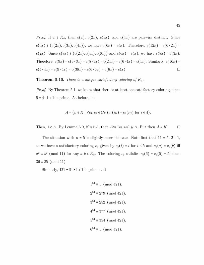
The situation with n = 5 is slightly more delicate. Note first that 11 = 5 ⋅ 2 + 1,
so we have a satisfactory coloring c5 given by c5(i) = i for i ≤ 5 and c5(a) = c5(b) iff
a2 ≡ b2 (mod 11) for any a, b ∈ K5. The coloring c5 satisfies c5(6) = c5(5) = 5, since
36 ≡ 25 (mod 11).
Similarly, 421 = 5 ⋅ 84 + 1 is prime and
184 ≡ 1 (mod 421),
284 ≡ 279 (mod 421),
384 ≡ 252 (mod 421),
484 ≡ 377 (mod 421),
584 ≡ 354 (mod 421),
684 ≡ 1 (mod 421),
43
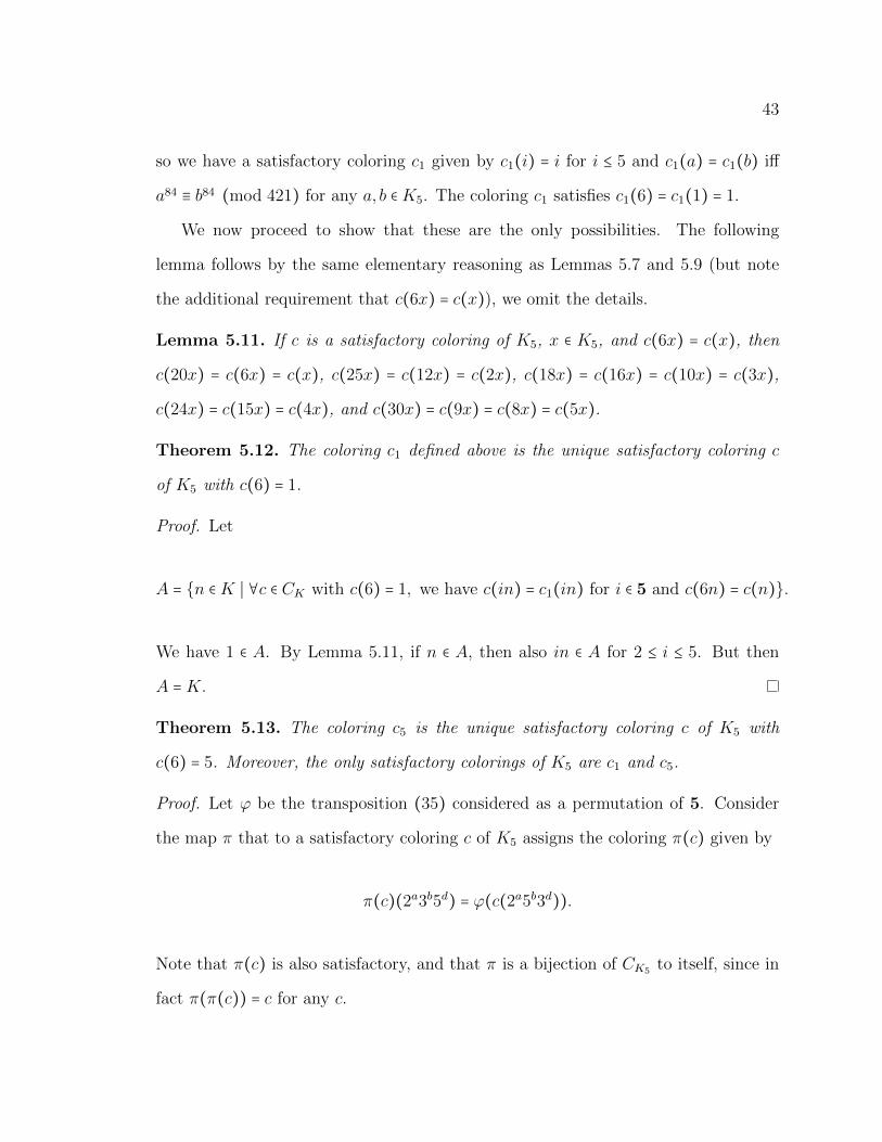
so we have a satisfactory coloring c1 given by c1(i) = i for i ≤ 5 and c1(a) = c1(b) iff
a84 ≡ b84 (mod 421) for any a, b ∈K5. The coloring c1 satisfies c1(6) = c1(1) = 1.
We now proceed to show that these are the only possibilities. The following
lemma follows by the same elementary reasoning as Lemmas 5.7 and 5.9 (but note
the additional requirement that c(6x) = c(x)), we omit the details.
Lemma 5.11. If c is a satisfactory coloring of K5, x ∈ K5, and c(6x) = c(x), then
c(20x) = c(6x) = c(x), c(25x) = c(12x) = c(2x), c(18x) = c(16x) = c(10x) = c(3x),
c(24x) = c(15x) = c(4x), and c(30x) = c(9x) = c(8x) = c(5x).
Theorem 5.12. The coloring c1 defined above is the unique satisfactory coloring c
of K5 with c(6) = 1.
Proof. Let
A = {n ∈K ∣ ∀c ∈ CK with c(6) = 1, we have c(in) = c1(in) for i ∈ 5 and c(6n) = c(n)}.
We have 1 ∈ A. By Lemma 5.11, if n ∈ A, then also in ∈ A for 2 ≤ i ≤ 5. But then
A =K.
Theorem 5.13. The coloring c5 is the unique satisfactory coloring c of K5 with
c(6) = 5. Moreover, the only satisfactory colorings of K5 are c1 and c5.
Proof. Let ϕ be the transposition (35) considered as a permutation of 5. Consider
the map π that to a satisfactory coloring c of K5 assigns the coloring π(c) given by
π(c)(2a3b5d) = ϕ(c(2a5b3d)).
Note that π(c) is also satisfactory, and that π is a bijection of CK5 to itself, since in
fact π(π(c)) = c for any c.
44
Suppose that c is satisfactory and c(6) = 5. Then, c(10) = 1. Otherwise, since
c(10) ∉ {c(2), c(4), c(6)} = {2,4,5}, we must have c(10) = 3. But then c(8) = 1.
Since c(12) ∉ {c(3), c(4), c(6), c(8)} = {1,3,4,5}, we must have c(12) = 2. But then
c(20) ∉ {c(4), c(5), c(8), c(10), c(12)} = {1,2,3,4,5}, a contradiction.
It follows that c(10) = 1 but then π(c)(6) = ϕ(c(10)) = ϕ(1) = 1 and therefore
π(c) = c1. Since π is injective, it follows that there is a unique c with c(6) = 5. But
then c = c5.
Finally, given any satisfactory coloring c of K5, since c(6) ∉ {c(2), c(3), c(4)} =
{2,3,4}, we must have that c(6) ∈ {1,5}, which implies that c = c1 or c = c5.
5.2.1 Density of Strong Representatives
In Section 5.2, we identified the colorings c5 and c1 (with associated primes 11 and
421, respectively) as being the only satisfactory colorings for n = 5. Note that there
are 76 primes in the interval [12,420] and none of them are strong representatives
of order 5. Now, it is only natural to ask whether 11 and 421 are the only strong
representatives of order 5. This is not the case:
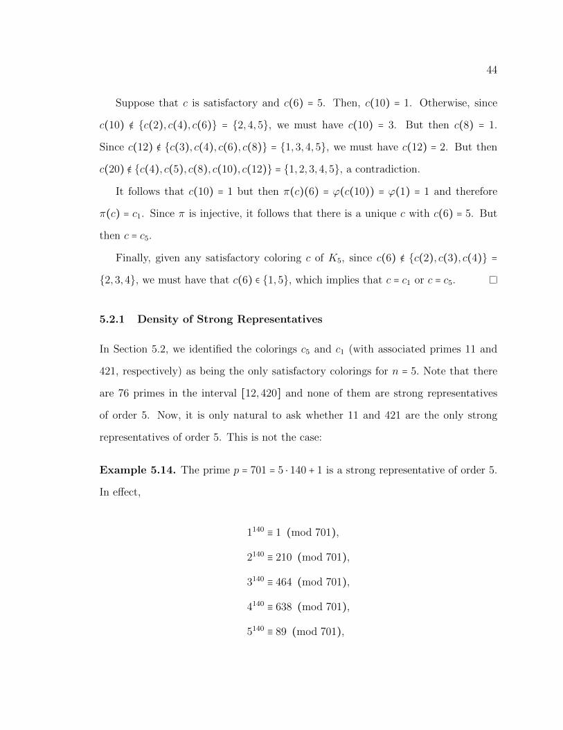
Example 5.14. The prime p = 701 = 5 ⋅ 140 + 1 is a strong representative of order 5.
In effect,
1140 ≡ 1 (mod 701),
2140 ≡ 210 (mod 701),
3140 ≡ 464 (mod 701),
4140 ≡ 638 (mod 701),
5140 ≡ 89 (mod 701),
45
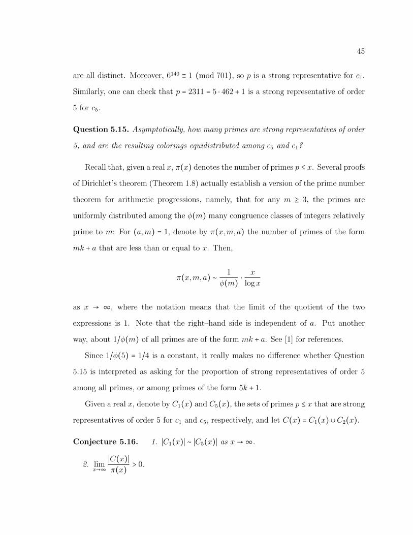
are all distinct. Moreover, 6140 ≡ 1 (mod 701), so p is a strong representative for c1.
Similarly, one can check that p = 2311 = 5 ⋅ 462 + 1 is a strong representative of order
5 for c5.
Question 5.15. Asymptotically, how many primes are strong representatives of order
5, and are the resulting colorings equidistributed among c5 and c1?
Recall that, given a real x, π(x) denotes the number of primes p ≤ x. Several proofs
of Dirichlet’s theorem (Theorem 1.8) actually establish a version of the prime number
theorem for arithmetic progressions, namely, that for any m ≥ 3, the primes are
uniformly distributed among the φ(m) many congruence classes of integers relatively
prime to m: For (a,m) = 1, denote by π(x,m,a) the number of primes of the form
mk + a that are less than or equal to x. Then,
π(x,m,a) ∼ 1
φ(m) ⋅x
logx
as x → ∞, where the notation means that the limit of the quotient of the two
expressions is 1. Note that the right–hand side is independent of a. Put another
way, about 1/φ(m) of all primes are of the form mk + a. See [1] for references.
Since 1/φ(5) = 1/4 is a constant, it really makes no difference whether Question
5.15 is interpreted as asking for the proportion of strong representatives of order 5
among all primes, or among primes of the form 5k + 1.
Given a real x, denote by C1(x) and C5(x), the sets of primes p ≤ x that are strong
representatives of order 5 for c1 and c5, respectively, and let C(x) = C1(x) ∪C2(x).
Conjecture 5.16. 1. ∣C1(x)∣ ∼ ∣C5(x)∣ as x→∞.
2. limx→∞
∣C(x)∣π(x) > 0.
46
Numerical data relevant to Conjecture 5.16 is shown in Appendix A.3. The Maple
code producing the data is listed as Figure A.3.
Of course, similar questions can be asked for any n in place of 5.
Recall that Question 5.6 asks whether strong representatives of all orders exist. It
is hard to imagine a scenario that would show the existence of strong representatives
of a given order n without proving that there are infinitely many. For n = 2, we can
prove that this is the case:
Theorem 5.17. A prime p is a strong representative of order 2 iff p ≡ ±3 (mod 8).
In particular, there are infinitely many strong representatives of order 2.
Proof. This is immediate from Theorem 1.10: If p = 2k + 1 is prime, then
2k ≡ 1 (mod p)
iff p ≡ ±1 (mod 8). It follows that if p ≡ ±3 (mod 8), then 1 and 2k are not congruent
modulo p.
Treating other cases seems to require a good understanding of higher order reci-
procity laws. An argument that would apply to all n seems even more delicate.2
5.3 k-representatives
Definition 5.18. Let k ∈ Z+. A prime p of the form nk + 1 is a k-representative if
and only if p is a strong representative of order n.
It is important to note that, in general, the roles of k and n cannot be interchanged.
That is, typically, if p = nk + 1 is a strong representative of order n, then it is not
2See Section 7.2.
47
an n-representative, and if it is a k-representative, it is not a strong representative of
order k.
The goal of this section is to show that for every k > 2, there are only finitely
many n such that p = nk + 1 is a k-representative. In fact, we will show that for some
values of k there are no such n.
We begin by discussing the case k = 3.
Theorem 5.19. Suppose p = n3 + 1 is prime. Then, there is an i ∈ n, i > 2 such that
i3 ≡ 1 (mod p) or i3 ≡ 8 (mod p). In particular, p is not a 3-representative.
Proof. Note first that −3 is a quadratic residue modulo p. This follows from Theorem
1.9:
(−3
p) = (−1
p)(3
p) = (−1) p−1
2 (−1) p−12
3−12 (p
3) = (n3 + 1
3) = (1
3) = 1.
Work in Zp. Note that x3 = 1 and x ≠ 1 iff x2 + x + 1 = 0 iff 4x2 + 4x + 4 = 0 iff
(2x + 1)2 = −3. Also, x3 = 8 and x ≠ 2 iff x2 + 2x + 4 = 0, or (x + 1)2 = −3.
We claim that for at least one x ∈ n this must happen. This is because y2 = −3
has two solutions, one in the first half of the interval [1, p − 1]. If y is actually in the
first third, we are done, we get x = y − 1 ∈ n. Suppose otherwise. Note that either y
or p − y is odd. Call it z, and note that z ≤ 2p/3. But then x = (z − 1)/2 is at most
(p − 1)/3, so it is in n.
The case when k is a multiple of 4 can also be treated by elementary means. The
key is the following theorem of Fermat, see Theorem 13.3 in [1]:
Theorem 5.20. (Fermat) An odd prime p is a sum of two squares iff p ≡ 1 (mod 4).
Theorem 5.21. If k is a multiple of 4 and p = nk+1 is k-representative, then p < 2k2,
so in particular, there are only finitely many k-representatives.
48
Proof. Suppose p = nk + 1 is a k-representative. By Theorem 5.20, there are integers
x and y with 1 ≤ x < y such that p = x2 + y2. Fix an integer t. Then, if p > t2 (which
is true for all but finitely many p), then y ≤ p/t. Otherwise, p = x2 + y2 > y2 > p2/t2, a
contradiction.
It follows that if p ≥ 2k2, then both x and y are in n, but x2 ≡ −y2 (mod p), so
xk ≡ yk (mod p).
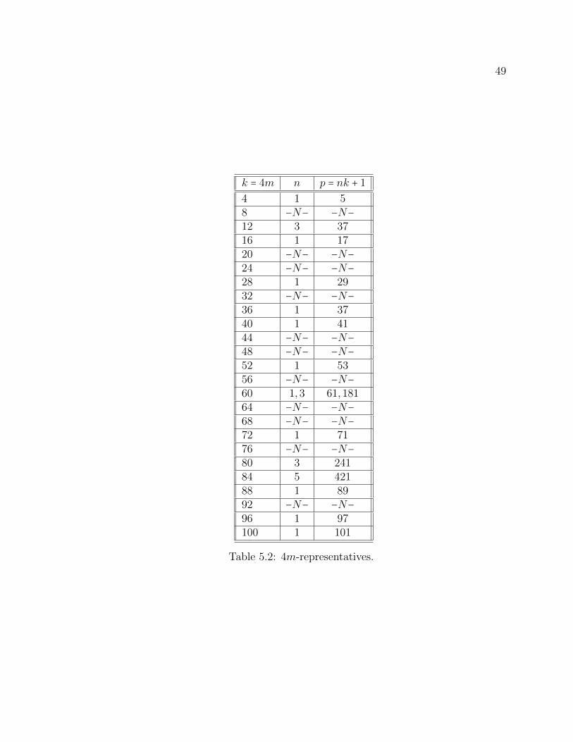
The bound on p found in Theorem 5.21 allows us for any given value of k = 4m to
identify all the possible values of p by a quick exhaustive search. Table 5.2 shows for
k = 4m ≤ 100 the values of n for which p = nk + 1 = n4m + 1 is a k-representative. If
there are no such primes, we write −N−.
We now proceed to the general case. Letting
B(t, x) = tetx
et − 1=
∞
∑m=0
Bm(x) tm
m!,
then
B(t, x + 1) = tetxet
et − 1= te
tx(et + 1 − 1)et − 1
= text +B(t, x).
Thus∞
∑m=0
(Bm(x + 1) −Bm(x)) tm
m!= text =
∞
∑m=0
mxm−1tm
m!,
or
Bm(x + 1) −Bm(x) =mxm−1.
It follows easily that each Bm(x) is a polynomial in x of degree m with rational
coefficients. Moreover, we have
49
k = 4m n p = nk + 1
4 1 58 −N− −N−12 3 3716 1 1720 −N− −N−24 −N− −N−28 1 2932 −N− −N−36 1 3740 1 4144 −N− −N−48 −N− −N−52 1 5356 −N− −N−60 1,3 61,18164 −N− −N−68 −N− −N−72 1 7176 −N− −N−80 3 24184 5 42188 1 8992 −N− −N−96 1 97100 1 101
Table 5.2: 4m-representatives.
50
n
∑i=0
Bm+1(i + 1) −Bm+1(i) =n
∑i=0
(m + 1)im,
orn
∑i=1
im = Bm(n + 1) −Bm+1(0)m + 1
.
A good reference on Bernoulli polynomials is [16]. Writing
Bm(x) =m
∑k=0
( m
m − k)bkxm−k,
the numbers bk = Bk(0) are usually called the Bernoulli numbers; they satisfy b2k+1 = 0
for all k ≥ 1. In particular,n
∑i=1
i2m = B2m+1(n + 1)2m + 1
,
for m ≥ 1.
It will be important for us to know all the rational linear factors of the polynomial
Bm(x)−Bm(0); when n is odd this reduces to determining the rational linear factors
of Bm(x). A theorem of Inkeri, see Theorem 3 in [17], solves this problem.
Theorem 5.22. (Inkeri) [17]
The rational roots of a Bernoulli polynomial Bm(x) can be only 0, 12 , and 1. Moreover,
all these are roots when m > 1 is odd.
With this result we are ready to prove the main result of this section.
Theorem 5.23. If k > 2, then only finitely many primes are k-representatives.
The following argument was suggested by Darij Grinberg and Gergely Harcos, see
[15].
51
Proof. Suppose p = nk + 1 is a k-representative, that is, p is a strong representative
of order n. We claim that
1k + 2k + . . . + nk ≡ 0 (mod p).
To see this, let S = 1k + . . .+ (p−1)k (mod p). Note that the map i↦ 2i (mod p) is a
permutation of p − 1. Therefore, S ≡ 2kS (mod p), so S ≡ 0 (mod p). By Theorem
1.6, any nonzero kth power is congruent to ik modulo p for some i ∈ n, and for each
such i there are precisely k integers in p − 1 realizing this congruence. But then
S ≡ k(1k + . . . + nk) (mod p), and the claim follows.
Similarly,n
∑i=1
i2k ≡ 0 (mod p).
To see this, notice that, again by Theorem 1.6, there are precisely p−1d = n
(2,n) incon-
gruent 2kth power residues modulo p, where d = (2k, p − 1) = (2, n)k. If n is odd,
this is precisely n, which means that the numbers 12k, . . . , n2k are all distinct and are
precisely all the nonzero 2kth powers. If n is even, this means that each nonzero 2kth
power appears exactly twice among these numbers. In either case, it follows that the
sum is zero by the same argument as in the previous paragraph.
Sincen
∑i=0
i2k = B2k+1(n + 1)2k + 1
,
it must be the case that (nk + 1)∣B2k+1(n+ 1). By Inkeri’s Theorem 5.22, since k > 2,
the polynomial kx + 1 is relatively prime to the polynomial B2k+1(x + 1). But then
there must be polynomials u, v ∈ Q[x] such that
52
(kx + 1) ⋅ u(x) +B2k+1(x + 1) ⋅ v(x) = 1.
(In fact, v is a constant.)
Multiplying this identity by an appropriate integer constant L = L1L2, it follows
that there are polynomials u′ = Lu,B′2k+1 = L1B2k+1, v′ = L2v ∈ Z[x] such that
(kx + 1) ⋅ u′(x) +B′2k+1(x + 1) ⋅ v′(x) = L.
Since B2k+1(n + 1) ≡ 0 (mod nk + 1), evaluating the last displayed equation at x = n
gives us that p = nk + 1∣L. But there are only finitely many such p.
Note that this argument does not supersede Theorems 5.19 or 5.21. For Theorem
5.21 in particular, note that the bound obtained there is in general much smaller than
the bound L found in the proof of Theorem 5.23, which depends on the size of the
denominator of B2k+1(x + 1). Let us illustrate this result with some examples.
Example 5.24.n
∑i=1
i3 = n2(n + 1)2
4.
Clearly, if n3+1 is prime, it does not divide n2(n+1)2. Thus, it follows that no prime
is a 3-representative.
Example 5.25.n
∑i=1
i4 = n(n + 1)(2n + 1)(3n2 + 3n − 1)30
.
If n4 + 1 is a 4-representative, then it must divide (3n2 + 3n − 1). But
16(3n2 + 3n − 1) = (9 + 12n)(n4 + 1) − 25,
53
so n4 + 1 must divide 25, so n = 1, and p = 5 is the only 4-representative.
Example 5.26.n
∑i=1
i5 = n2(n + 1)2(2n + 1)(2n2 + 2n − 1)
12.
If n5 + 1 is a 5-representative, then it must divide (2n2 + 2n − 1). But
25(2n2 + 2n − 1) = (10n + 8)(n5 + 1) − 33,
so n5 + 1 must divide 33, so n = 2. Since
25 = 32 ≡ −1 ≢ 1 (mod 11),
it follows that p = 11 is indeed the only 5-representative.
Example 5.27.
n
∑i=1
i6 = n(n + 1)(2n + 1)(3n4 + 6n3 − 3n + 1)42
.
If n6 + 1 is a 6-representative, then it must divide (3n4 + 6n3 − 3n + 1). But
432(3n4 + 6n3 − 3n + 1) = (216n3 + 396n2 − 66n − 205)(n6 + 1) + 637,
so n6 + 1 must divide 637 = 72 ⋅ 13, so n = 1 or n = 2. Since
26 = 64 ≡ −1 ≢ 1 (mod 13),
it follows that p = 7 and p = 13 are the only 6-representatives.
54
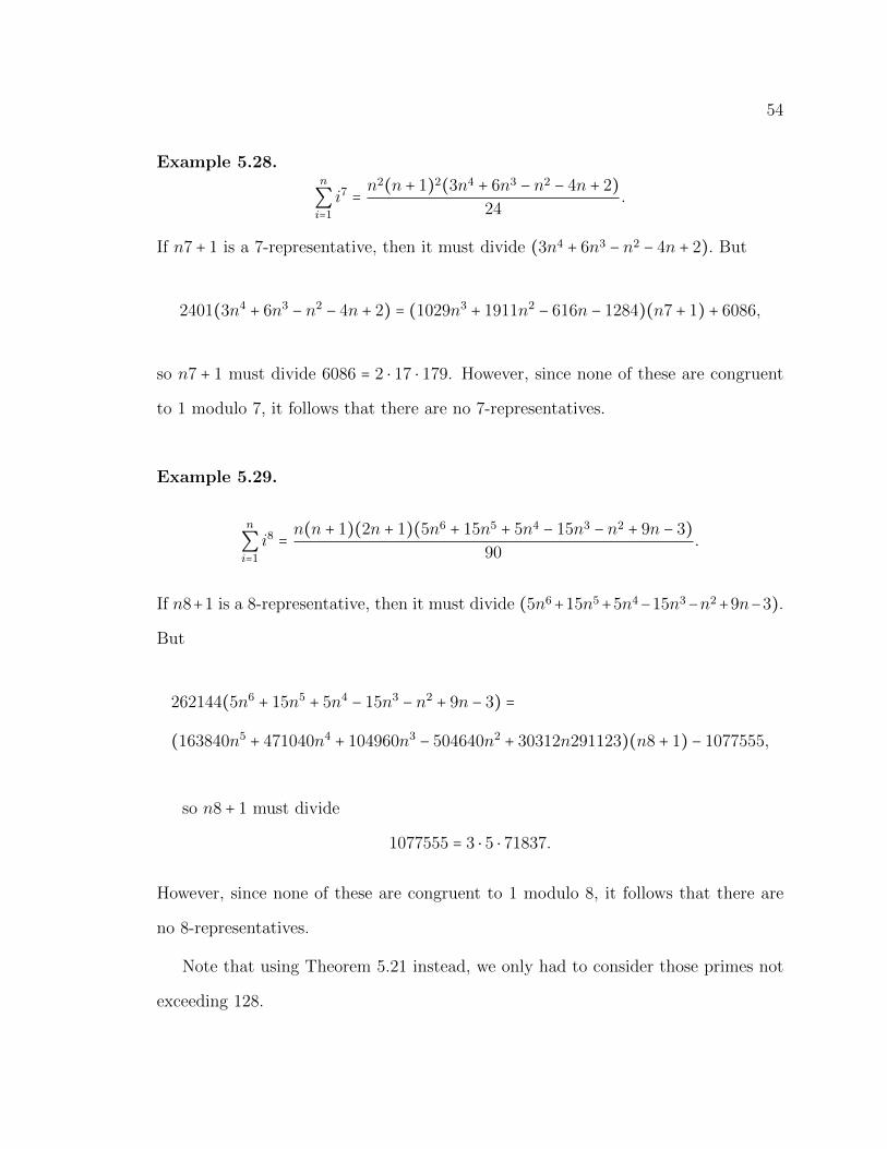
Example 5.28.n
∑i=1
i7 = n2(n + 1)2(3n4 + 6n3 − n2 − 4n + 2)
24.
If n7 + 1 is a 7-representative, then it must divide (3n4 + 6n3 − n2 − 4n + 2). But
2401(3n4 + 6n3 − n2 − 4n + 2) = (1029n3 + 1911n2 − 616n − 1284)(n7 + 1) + 6086,
so n7 + 1 must divide 6086 = 2 ⋅ 17 ⋅ 179. However, since none of these are congruent
to 1 modulo 7, it follows that there are no 7-representatives.
Example 5.29.
n
∑i=1
i8 = n(n + 1)(2n + 1)(5n6 + 15n5 + 5n4 − 15n3 − n2 + 9n − 3)90
.
If n8+1 is a 8-representative, then it must divide (5n6+15n5+5n4−15n3−n2+9n−3).
But
262144(5n6 + 15n5 + 5n4 − 15n3 − n2 + 9n − 3) =
(163840n5 + 471040n4 + 104960n3 − 504640n2 + 30312n291123)(n8 + 1) − 1077555,
so n8 + 1 must divide
1077555 = 3 ⋅ 5 ⋅ 71837.
However, since none of these are congruent to 1 modulo 8, it follows that there are
no 8-representatives.
Note that using Theorem 5.21 instead, we only had to consider those primes not
exceeding 128.
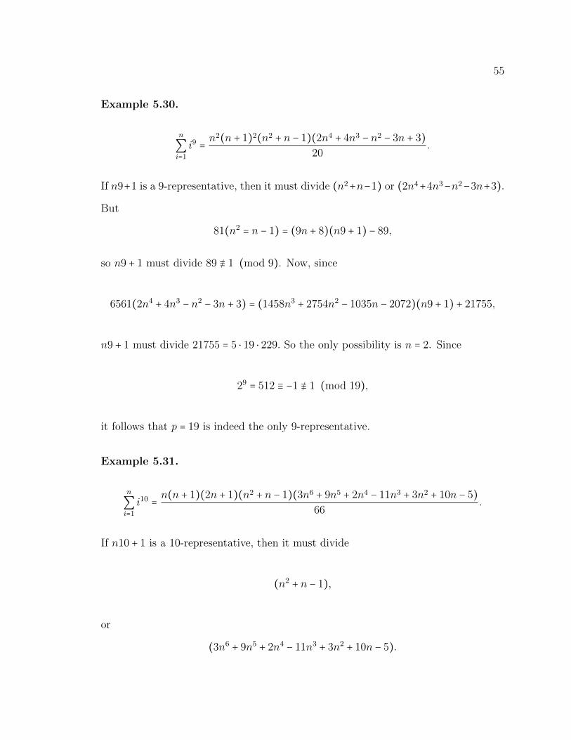
55
Example 5.30.
n
∑i=1
i9 = n2(n + 1)2(n2 + n − 1)(2n4 + 4n3 − n2 − 3n + 3)
20.
If n9+1 is a 9-representative, then it must divide (n2+n−1) or (2n4+4n3−n2−3n+3).
But
81(n2 = n − 1) = (9n + 8)(n9 + 1) − 89,
so n9 + 1 must divide 89 ≢ 1 (mod 9). Now, since
6561(2n4 + 4n3 − n2 − 3n + 3) = (1458n3 + 2754n2 − 1035n − 2072)(n9 + 1) + 21755,
n9 + 1 must divide 21755 = 5 ⋅ 19 ⋅ 229. So the only possibility is n = 2. Since
29 = 512 ≡ −1 ≢ 1 (mod 19),
it follows that p = 19 is indeed the only 9-representative.
Example 5.31.
n
∑i=1
i10 = n(n + 1)(2n + 1)(n2 + n − 1)(3n6 + 9n5 + 2n4 − 11n3 + 3n2 + 10n − 5)66
.
If n10 + 1 is a 10-representative, then it must divide
(n2 + n − 1),
or
(3n6 + 9n5 + 2n4 − 11n3 + 3n2 + 10n − 5).
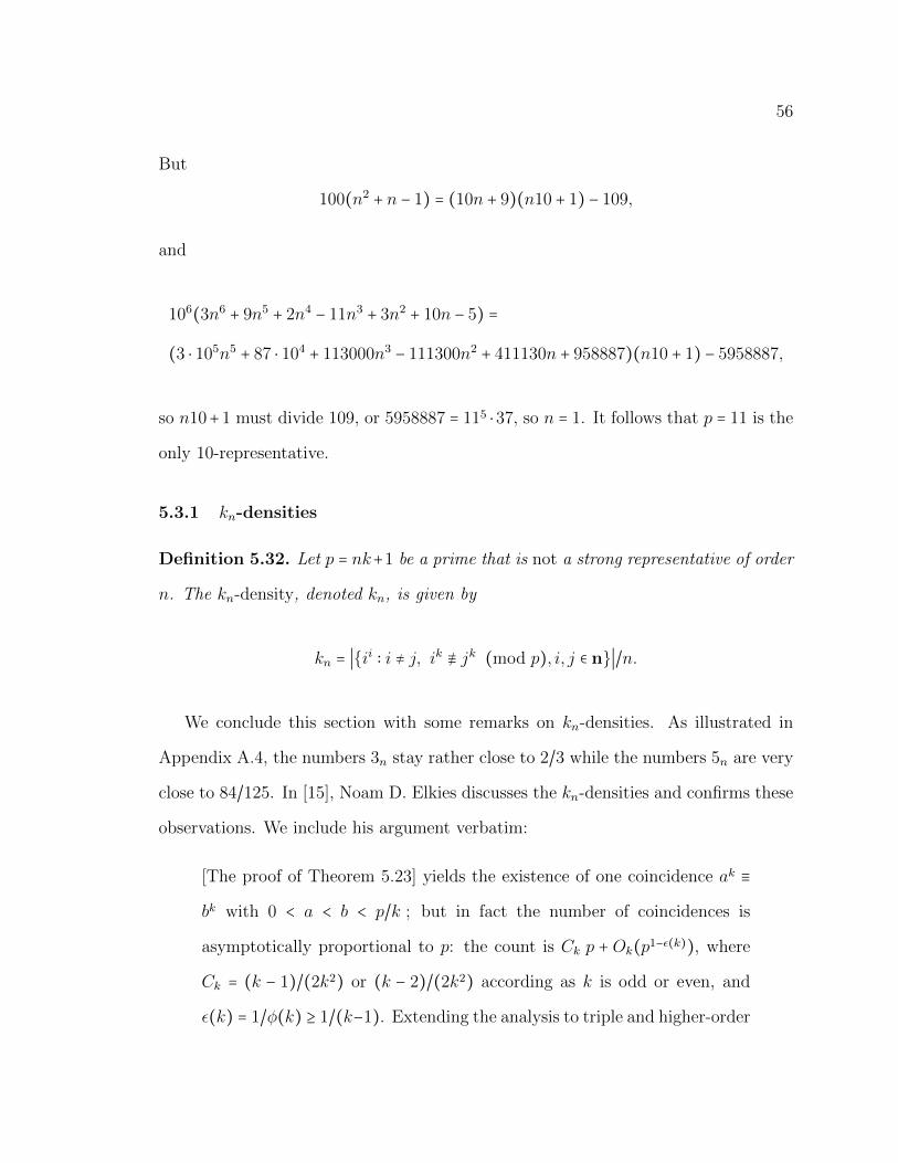
56
But
100(n2 + n − 1) = (10n + 9)(n10 + 1) − 109,
and
106(3n6 + 9n5 + 2n4 − 11n3 + 3n2 + 10n − 5) =
(3 ⋅ 105n5 + 87 ⋅ 104 + 113000n3 − 111300n2 + 411130n + 958887)(n10 + 1) − 5958887,
so n10+1 must divide 109, or 5958887 = 115 ⋅37, so n = 1. It follows that p = 11 is the
only 10-representative.
5.3.1 kn-densities
Definition 5.32. Let p = nk+1 be a prime that is not a strong representative of order
n. The kn-density, denoted kn, is given by
kn = ∣{ii ∶ i ≠ j, ik ≢ jk (mod p), i, j ∈ n}∣/n.
We conclude this section with some remarks on kn-densities. As illustrated in
Appendix A.4, the numbers 3n stay rather close to 2/3 while the numbers 5n are very
close to 84/125. In [15], Noam D. Elkies discusses the kn-densities and confirms these
observations. We include his argument verbatim:
[The proof of Theorem 5.23] yields the existence of one coincidence ak ≡
bk with 0 < a < b < p/k ; but in fact the number of coincidences is
asymptotically proportional to p: the count is Ck p + Ok(p1−ε(k)), where
Ck = (k − 1)/(2k2) or (k − 2)/(2k2) according as k is odd or even, and
ε(k) = 1/φ(k) ≥ 1/(k−1). Extending the analysis to triple and higher-order
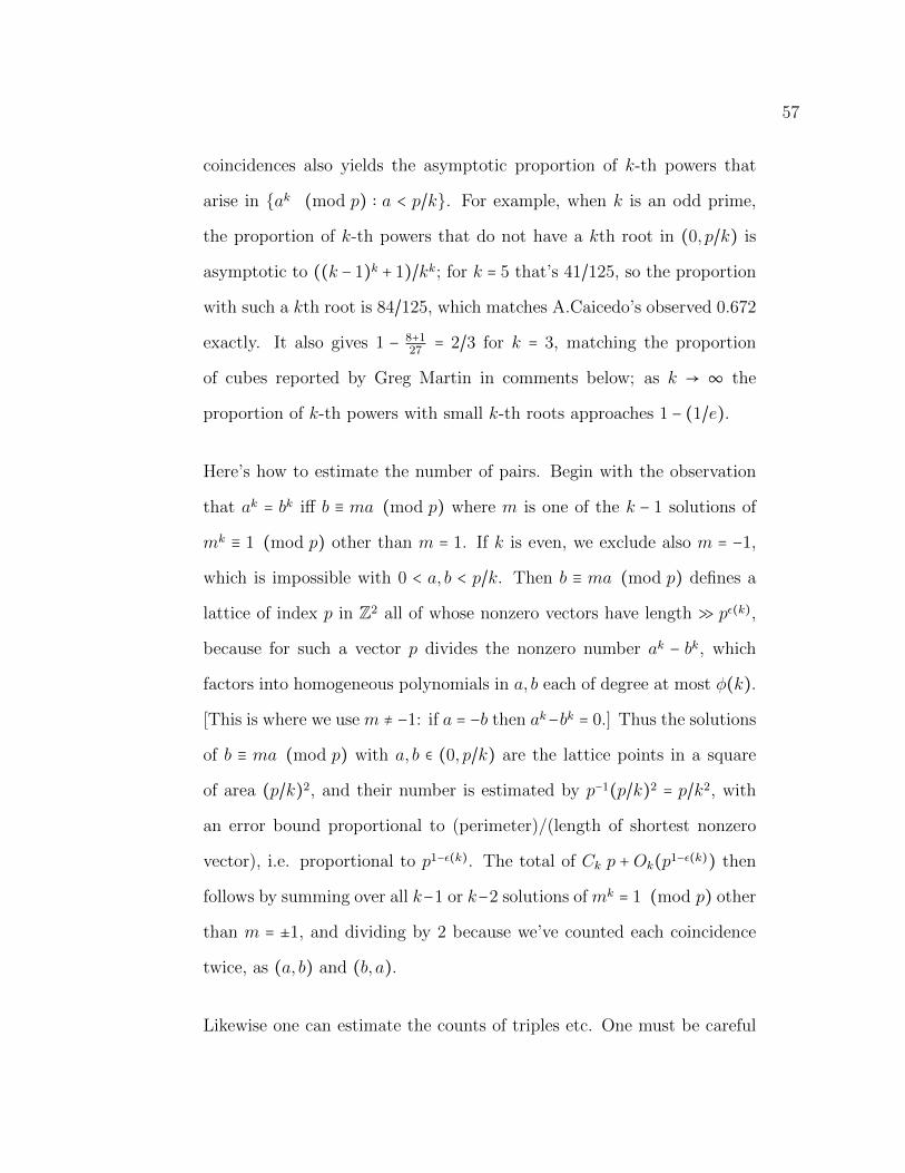
57
coincidences also yields the asymptotic proportion of k-th powers that
arise in {ak (mod p) ∶ a < p/k}. For example, when k is an odd prime,
the proportion of k-th powers that do not have a kth root in (0, p/k) is
asymptotic to ((k − 1)k + 1)/kk; for k = 5 that’s 41/125, so the proportion
with such a kth root is 84/125, which matches A.Caicedo’s observed 0.672
exactly. It also gives 1 − 8+127 = 2/3 for k = 3, matching the proportion
of cubes reported by Greg Martin in comments below; as k → ∞ the
proportion of k-th powers with small k-th roots approaches 1 − (1/e).
Here’s how to estimate the number of pairs. Begin with the observation
that ak = bk iff b ≡ ma (mod p) where m is one of the k − 1 solutions of
mk ≡ 1 (mod p) other than m = 1. If k is even, we exclude also m = −1,
which is impossible with 0 < a, b < p/k. Then b ≡ ma (mod p) defines a
lattice of index p in Z2 all of whose nonzero vectors have length ≫ pε(k),
because for such a vector p divides the nonzero number ak − bk, which
factors into homogeneous polynomials in a, b each of degree at most φ(k).
[This is where we use m ≠ −1: if a = −b then ak−bk = 0.] Thus the solutions
of b ≡ ma (mod p) with a, b ∈ (0, p/k) are the lattice points in a square
of area (p/k)2, and their number is estimated by p−1(p/k)2 = p/k2, with
an error bound proportional to (perimeter)/(length of shortest nonzero
vector), i.e. proportional to p1−ε(k). The total of Ck p +Ok(p1−ε(k)) then
follows by summing over all k−1 or k−2 solutions of mk = 1 (mod p) other
than m = ±1, and dividing by 2 because we’ve counted each coincidence
twice, as (a, b) and (b, a).
Likewise one can estimate the counts of triples etc. One must be careful
58
with subsets of the kth roots of unity that have integer dependencies,
but at least when k is prime there are no dependencies except that all
k of them sum to zero. If I did this right, the result for j < k is that
the number of j-element subsets of {1,2, . . . , (p−1)/k} with the same kth
power is asymptotic to (kj)p/kj+1, while there are no such subsets with
j = k because the sum of all k solutions of ak ≡ c (mod p) vanishes. An
exercise in generatingfunctionological inclusion-exclusion then produces
the formula ((k − 1)k + 1)/kk for the asymptotic proportion of kth powers
that have no kth roots at all in (0, p/k).
The same technique also works for 0 < a < b < M with M considerably
smaller than p/k; and the resulting coincidences, when they exist, can be
calculated efficiently using lattice basis reduction (which as it happens I
mentioned on this forum [http://mathoverflow.net/questions/77986] a few
days ago).
5.4 Multiplicative Colorings
As shown in Section 5.2, if n ≤ 5, then any satisfactory coloring of Kn admits a strong
representation. These colorings are very special: Fix some n, and suppose that c is
a satisfactory coloring of Kn admitting a strong representation ϕ associated to the
prime p = nk + 1. Let G = {ak (mod p) ∣ a ∈ n}. Then, as pointed out in Corollary
1.7, G ≤ Z∗p is a group isomorphic to Zn. Let h = ϕ ○ c, so
h ∶Kn → G.
Since h(a) = ak (mod p) for any a ∈Kn, the map h satisfies
59
h(ab) = h(a) ⋅ h(b)
for any a, b ∈ Kn, where ab is the usual product of a and b and h(a) ⋅ h(b) is the
product in G. Note that the bijection ϕ coincides with the restriction of h to n.
Definition 5.33. A satisfactory coloring c of Kn is multiplicative iff there exists a
group (G, ⋅) of order n and a bijection ϕ ∶ n → G such that, letting h = ϕ ○ c, we have
that
h(ab) = h(a) ⋅ h(b)
for any a, b ∈Kn. In this case, we say that c is a G-coloring.
Lemma 5.34. If a satisfactory coloring of Kn is both a G1-coloring and a G2-coloring,
then G1 ≅ G2.
Proof. If ϕ1 ∶ n → G1 and ϕ2 ∶ n → G2 witness that c is both a G1-coloring and a
G2-coloring, then ϕ1 ○ ϕ−12 ∶ G2 → G1 is an isomorphism.
Note that if G is as in Definition 5.33, then G is abelian, and consequently we
adopt additive notation in what follows, so h is a kind of discrete logarithm. Rather
than adopting this notation, we also say that h is multiplicative:
Definition 5.35. If (G,+) is an abelian group and the map h ∶Kn → G satisfies that
h(ab) = h(a) + h(b) for any a, b ∈Kn, we say that h is multiplicative.
Since there are only finitely many groups of any given order, there are only finitely
many possibilities for G. In fact, we can easily list all the possibilities, thanks to the
classification theorem for finite abelian groups, Theorem 4.3 in [1]:
Theorem 5.36. Any finite abelian group is isomorphic to a direct sum of the form
Zn1 ×⋯ ×Znkwhere each ni is a power of a prime number.
60
Corollary 5.37. For any n, there are only finitely many multiplicative colorings of
Kn.
Proof. Suppose c is multiplicative as witnessed by (G,+), ϕ. Let h = ϕ ○ c, so h(ab) =
h(a)+h(b) for all a, b ∈Kn. Note that this induces a group structure ⊕ on n isomorphic
to G because c is the identity on n, so if a ∈ n, then h(a) = ϕ(c(a)) = ϕ(a). So we
are setting a ⊕ b = d for a, b, d ∈ n, if and only if ϕ(d) = ϕ(a) + ϕ(b). By identifying
(G,+) with (n,⊕), it follows that we may assume that ϕ is the identity so h = c. But
then (n,⊕) completely determines c. In effect, if p1, . . . , pk are the primes less than
or equal to n, then the multiplicity requirement gives us
c(pα11 ⋯pαk
k ) = α1c(p1)⊕ . . .⊕ αkc(pk),
where
αic(pi) = c(pi)⊕ . . .⊕ c(pi)´¹¹¹¹¹¹¹¹¹¹¹¹¹¹¹¹¹¹¹¹¹¹¹¹¹¹¹¹¹¹¹¹¹¹¹¹¹¹¹¹¹¹¹¹¹¹¹¹¸¹¹¹¹¹¹¹¹¹¹¹¹¹¹¹¹¹¹¹¹¹¹¹¹¹¹¹¹¹¹¹¹¹¹¹¹¹¹¹¹¹¹¹¹¹¹¹¹
αi times
.
Since there are only finitely many group structures on n, we are done.
In what follows, given an abelian group (G,⊕), we will denote α-fold sums of the
form
g ⊕⋯⊕ g´¹¹¹¹¹¹¹¹¹¹¹¹¹¹¹¹¹¸¹¹¹¹¹¹¹¹¹¹¹¹¹¹¹¹¹¶α times
by g⊕α.
Remark 5.38. Note that not every abelian group structure of n gives rise to a
multiplicative coloring. For example, by Theorem 5.10, if n = 4, then ⊕ is given by
a ⊕ b = ab (mod 5) and in particular ⊕ is isomorphic to Z4 and not to Z2 × Z2. We
further discuss this in the next chapter.
61
The case when G ≅ Zn, as in the case of a strong representation, deserves special
attention.
Question 5.39. Does every Zn-coloring admit a strong representation?
Perhaps surprisingly, the answer to Question 5.39 is negative, as we show in the
next chapter. Nevertheless, we can answer Question 5.39 affirmatively at the cost of
replacing strong representations with a weak variant, see Remark 5.46.
Although so far our examples and results have only exhibited multiplicative col-
orings, it should be pointed out that not every satisfactory coloring is multiplicative.
For example, in personal communication, Caicedo has found a non-multiplicative
satisfactory coloring of K6. We state the result without proof.
Theorem 5.40. (Caicedo)
There is a unique satisfactory coloring c of K6 such that c(23) = 5, c(24) = 2, c(25) = 4,
c(32) = 9, c(26n) = c(n), c(12n) = c(27n), and c(20n) = c(45n) for any n ∈ K6. This
coloring satisfies that c(37n) = c(3n) and c(57n) = c(5n) for any n ∈K6.
Note that if c is as in Theorem 5.40, then it is non-multiplicative. For example, if
c is multiplicative, then c(18) = c(9×2) = c(9)+c(2) = c(2)+c(2) = c(2×2) = c(4) = 4.
Instead, c(18) = 5.
Similarly, not every multiplicative coloring is a Zn-coloring. Examples are pre-
sented in the next chapter. Non-multiplicative colorings seem more difficult to ana-
lyze, and we do not understand them well. For example, the coloring c from Theorem
5.40 is periodic, in the sense that c(p7n) = c(pn) for p = 2,3,5 and n ∈ K6; we do not
know whether there are non-periodic non-multiplicative colorings as well. In what
follows, we restrict our attention to the multiplicative case.
62
5.5 Partial G-Homomorphisms
The following extends a notion due independently to Caicedo and Ewan Delanoy, see
[2], where only the case G = Zn was considered. Though not identical, it is closely
related to the concept of Freiman homomorphism in additive combinatorics, see [5].
Definition 5.41. Let (G,+) be an abelian group of order n. A map h ∶ n → G is
a partial G-homomorphism if and only if h is a bijection and, whenever a, b ∈ n, if
ab ≤ n, then h(ab) = h(a)+h(b). If G = Zn, we simply call h a partial homomorphism.
Remark 5.42. We require G to be abelian as our goal is to relate partial G-
homomorphisms to satisfactory colorings, cf. Theorem 5.43 below, and the natural
argument, requires that G is abelian. But the question of whether there are partial
G-homomorphisms where G is not abelian is interesting in its own right. This seems to
be open in general, but for n odd the answer is negative, as shown by K.A. Chandler,
see [24].
Since h is a bijection, it induces a group operation ⊕ on n such that (n,⊕) ≅
(G,+) and ⊕ extends the partial graph of multiplication on n. Our use of the
phrase homomorphism here is based on the following observation: For any partial
G-homomorphism h, we have that h(1) = h(1 ⋅ 1) = h(1) + h(1) = h(1)⊕2. It follows
that h(1) = 0G. In other words, h maps the multiplicative identity in n to the additive
identity in G, and embeds a multiplicative structure into an additive one.
Theorem 5.43. If h ∶ n → G is a partial G-homomorphism, then h can be uniquely
extended to a multiplicative map h ∶ Kn → G. Moreover, h−1 ○ h ∶ Kn → n is a
G-coloring of Kn.
63
Proof. Let h ∶ n → G be a partial G-homomorphism. Let p1, . . . , ps be the primes
less than or equal to n. Then, h ∶ Kn → G extends h and is multiplicative iff for any
a1, . . . , as ∈ N, we have
h(pa11 . . . pass ) =⊕i
h(pi)⊕iai .
This proves the existence and uniqueness of the extension h. Moreover, if 1 ≤ i < j ≤ n
and a ∈Kn, then
h(ia) = h(i) + h(a) ≠ h(j) + h(a) = h(ja)
because h ↾n= h is a bijection.
But then, letting c = h−1 ○ h, we have that c ∶Kn → n is a G-coloring.
Remark 5.44. Note the similarity between this argument and the proof of Corollary
5.37.
Obviously, if h ∶ Kn → G is multiplicative and h = h ↾n is a bijection, then h is a
partial G-homomorphism. Therefore, if c ∶Kn → n is a G-coloring as witnessed by the
bijection ϕ ∶ n → G, then ϕ is a partial G-homomorphism as, by definition, h = ϕ ○ c
is multiplicative, and ϕ = h ↾n.
This shows that the problem of building G-colorings of Kn is equivalent to the
problem of building partial G-homomorphisms or, equivalently, G-satisfactory groups:
Definition 5.45. Given an abelian group (G,+) of order n, we say that an abelian
group structure on n, (n,⊕), is a G-satisfactory group iff (n,⊕) ≅ (G,+) and a⊕b = ab
whenever a, b, ab ∈ n.
We say that the G-coloring resulting from extending ⊕ as in Theorem 5.43 is
associated to (n,⊕).
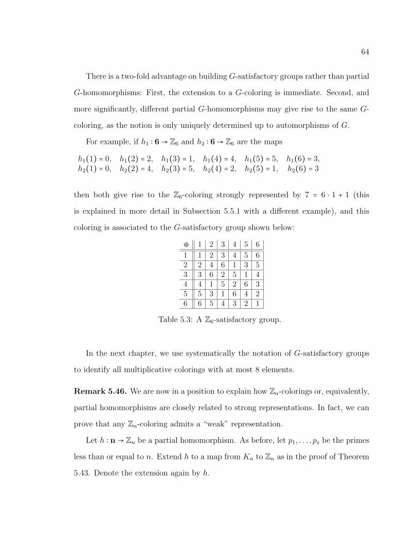
64
There is a two-fold advantage on building G-satisfactory groups rather than partial
G-homomorphisms: First, the extension to a G-coloring is immediate. Second, and
more significantly, different partial G-homomorphisms may give rise to the same G-
coloring, as the notion is only uniquely determined up to automorphisms of G.
For example, if h1 ∶ 6→ Z6 and h2 ∶ 6→ Z6 are the maps
h1(1) = 0, h1(2) = 2, h1(3) = 1, h1(4) = 4, h1(5) = 5, h1(6) = 3,h2(1) = 0, h2(2) = 4, h2(3) = 5, h2(4) = 2, h2(5) = 1, h2(6) = 3
then both give rise to the Z6-coloring strongly represented by 7 = 6 ⋅ 1 + 1 (this
is explained in more detail in Subsection 5.5.1 with a different example), and this
coloring is associated to the G-satisfactory group shown below:
⊕ 1 2 3 4 5 6
1 1 2 3 4 5 62 2 4 6 1 3 53 3 6 2 5 1 44 4 1 5 2 6 35 5 3 1 6 4 26 6 5 4 3 2 1
Table 5.3: A Z6-satisfactory group.
In the next chapter, we use systematically the notation of G-satisfactory groups
to identify all multiplicative colorings with at most 8 elements.
Remark 5.46. We are now in a position to explain how Zn-colorings or, equivalently,
partial homomorphisms are closely related to strong representations. In fact, we can
prove that any Zn-coloring admits a “weak” representation.
Let h ∶ n→ Zn be a partial homomorphism. As before, let p1, . . . , ps be the primes
less than or equal to n. Extend h to a map from Kn to Zn as in the proof of Theorem
5.43. Denote the extension again by h.
65
By Dirichlet’s theorem, there are primes P of the form nk+1. For any such P , let
g be a primitive root modulo P , i.e., a generator of Z∗P . In other words, the powers gki
are precisely the kth power residues modulo P . Invoking again Dirichlet’s theorem,
for each pi, we can find a prime qi such that qi ≡ gh(pi) (mod P ). Now for x ∈ Kn
define d ∶Kn → Z∗P by d(x) = gkh(x).
Suppose x =∏si=1 p
aii . Then, h(x) = ∑i aih(pi) and
d(x) =∏i
(gh(pi))kai = (∏i
qaii )k
(5.1)
where of course the products are computed modulo P .
The point is that if i, j ∈ n, then d(i) ≠ d(j) because h(i) ≠ h(j), h being a
bijection. Say 0 ≤ h(i) < h(j) < n, then 0 ≤ kh(i) < kh(j) < kn, and gkh(i) ≠ gkh(j),
since g is a primitive root. It follows that d(ix) = d(i)d(x) ≠ d(j)d(x) = d(jx) and,
after precomposing with an appropriate permutation, d becomes a Zn-coloring.
Note how close the coloring given by Equation 5.1 is to the colorings described in
Definition 5.2. Strong representations are the particular case where we can choose P
for which we can take qi = pi for all i.
Partial homomorphisms are easy to construct “by hand.” For instance, it is a
matter of at most a couple of hours to construct partial homomorphisms for all
n ≤ 32, essentially by what amounts to following a greedy algorithm. Examples of
partial homomorphisms for all n ≤ 54 are shown in Appendix B.3
Given n, define M and MKn as the sets of multiplicative colorings of Z+ and of
Kn, respectively. In Corollary 5.37, we showed that MKn is finite. We now show that
3See Section 7.2.
66
restricting attention to colorings in M does not affect the computation of the number
of satisfactory colorings, Corollary 4.7.
Theorem 5.47. If n > 1 and MK ≠ ∅, then ∣M ∣ = ∣R∣.
Proof. As in Corollary 4.7, it is enough to show that n∣N∣ ≤ ∣M ∣. Let c ∶ Kn → n be a
multiplicative coloring associated to the G-satisfactory group (n,⊕). To each prime
p assign a number ap ∈ n with the only restriction that ap = p if p ∈ n. Now define
c′ ∶ Z+ → n as follows: If m ∈ Z+, let ∏i pbii be its prime factorization, and set
c′(m) =⊕i
a⊕bipi.
It is immediate that any c′ defined this way is multiplicative and extends c, and that
different sequences (ap ∣ p prime) give rise to different c′. But then we have associated
n∣N∣ colorings in M to each c ∈MK , so n∣N∣ ≤ ∣M ∣.
5.5.1 An Example
Here we illustrate how to construct a satisfactory coloring of K5 by making use of
a partial homomorphism. To do so, we will again make use of the table described
in Chapter 4, but limited to columns in K5. However, in this case we will not view
the choices for first column as completely arbitrary. Instead, the first column will be
formed by creating a partial homomorphism.
Thus, we begin by forming a partial homomorphism h ∶ 5 → Z5. As we stated
above, h(1) = 0. Next, we will choose h(2) = 1. By choosing h(2) = 1, since h(4) =
h(2 ⋅ 2) = h(2) + h(2), we must define h(4) = 1 + 1 = 2. This leaves us to define h(3)
and h(5). Since 3 ⋅ 2 = 6 > 5 = n and 5 ⋅ 2 = 10 > 5 = n, we are free to choose any of
the remaining values as the image of 3 and 5. For simplicity, we will choose h(3) = 3
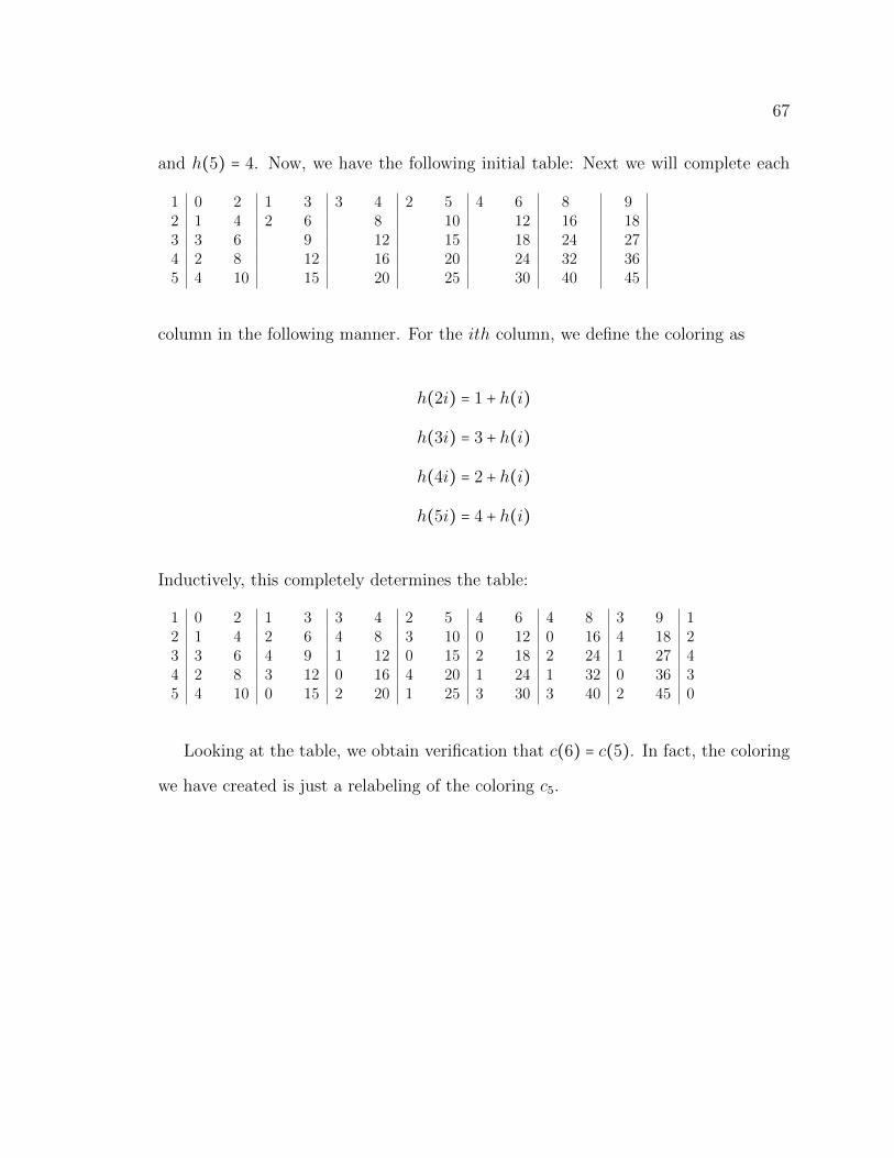
67
and h(5) = 4. Now, we have the following initial table: Next we will complete each
1 0 2 1 3 3 4 2 5 4 6 8 92 1 4 2 6 8 10 12 16 183 3 6 9 12 15 18 24 274 2 8 12 16 20 24 32 365 4 10 15 20 25 30 40 45
column in the following manner. For the ith column, we define the coloring as
h(2i) = 1 + h(i)
h(3i) = 3 + h(i)
h(4i) = 2 + h(i)
h(5i) = 4 + h(i)
Inductively, this completely determines the table:
1 0 2 1 3 3 4 2 5 4 6 4 8 3 9 12 1 4 2 6 4 8 3 10 0 12 0 16 4 18 23 3 6 4 9 1 12 0 15 2 18 2 24 1 27 44 2 8 3 12 0 16 4 20 1 24 1 32 0 36 35 4 10 0 15 2 20 1 25 3 30 3 40 2 45 0
Looking at the table, we obtain verification that c(6) = c(5). In fact, the coloring
we have created is just a relabeling of the coloring c5.
68
CHAPTER 6
MULTIPLICATIVE COLORINGS WITH AT MOST 8
COLORS
6.1 Six Colors
In this chapter, we build all G-satisfactory groups for 6 ≤ ∣G∣ ≤ 8, thus determining
all multiplicative colorings with at most 8 colors. See Section 5.5 for details on how
a G-satisfactory group (n,⊕) uniquely determines a G-coloring of Kn.
Note that the only abelian group of order 6 is Z6 ≅ Z2 × Z3 by Theorem 5.36, so
all the groups (6,⊕) we build here are Z6-satisfactory.
In the task of constructing the group operations ⊕ (extending the graph of mul-
tiplication on 6), the following immediate fact proves useful:
Fact 6.1. If (n,⊕) is G-satisfactory for some G, then {2⊕a ∣ a ∈ n,2a > n} coincides
with the set of odd integers in n.
Before we do anything, note the following base operation table for n = 6 (Table
6.1) is already determined, and our task is to fill out its blank spots.
It is also useful to keep in mind the following observations:
a. ⊕ must be associative and commutative.
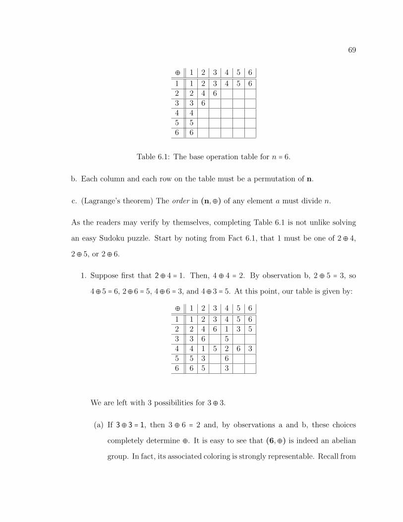
69
⊕ 1 2 3 4 5 6
1 1 2 3 4 5 62 2 4 63 3 64 45 56 6
Table 6.1: The base operation table for n = 6.
b. Each column and each row on the table must be a permutation of n.
c. (Lagrange’s theorem) The order in (n,⊕) of any element a must divide n.
As the readers may verify by themselves, completing Table 6.1 is not unlike solving
an easy Sudoku puzzle. Start by noting from Fact 6.1, that 1 must be one of 2 ⊕ 4,
2⊕ 5, or 2⊕ 6.
1. Suppose first that 2⊕ 4 = 1. Then, 4 ⊕ 4 = 2. By observation b, 2 ⊕ 5 = 3, so
4⊕ 5 = 6, 2⊕ 6 = 5, 4⊕ 6 = 3, and 4⊕ 3 = 5. At this point, our table is given by:
⊕ 1 2 3 4 5 6
1 1 2 3 4 5 62 2 4 6 1 3 53 3 6 54 4 1 5 2 6 35 5 3 66 6 5 3
We are left with 3 possibilities for 3⊕ 3.
(a) If 3⊕ 3 = 1, then 3 ⊕ 6 = 2 and, by observations a and b, these choices
completely determine ⊕. It is easy to see that (6,⊕) is indeed an abelian
group. In fact, its associated coloring is strongly representable. Recall from
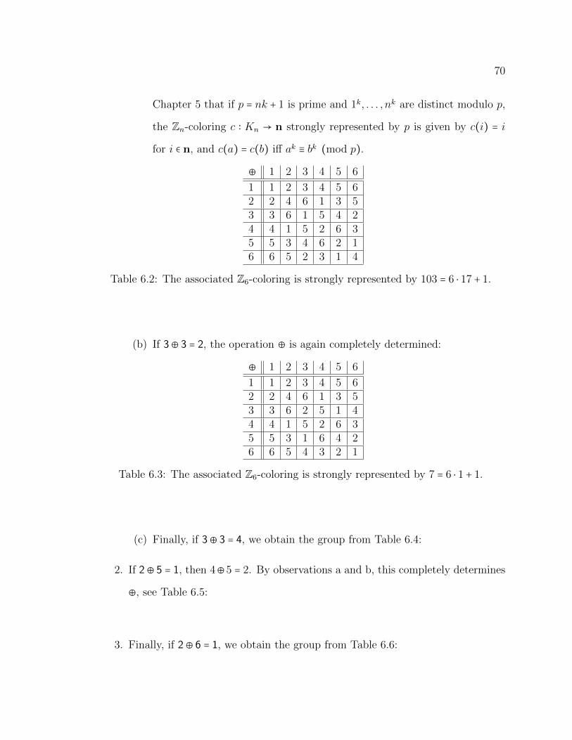
70
Chapter 5 that if p = nk + 1 is prime and 1k, . . . , nk are distinct modulo p,
the Zn-coloring c ∶ Kn → n strongly represented by p is given by c(i) = i
for i ∈ n, and c(a) = c(b) iff ak ≡ bk (mod p).
⊕ 1 2 3 4 5 6
1 1 2 3 4 5 62 2 4 6 1 3 53 3 6 1 5 4 24 4 1 5 2 6 35 5 3 4 6 2 16 6 5 2 3 1 4
Table 6.2: The associated Z6-coloring is strongly represented by 103 = 6 ⋅ 17 + 1.
(b) If 3⊕ 3 = 2, the operation ⊕ is again completely determined:
⊕ 1 2 3 4 5 6
1 1 2 3 4 5 62 2 4 6 1 3 53 3 6 2 5 1 44 4 1 5 2 6 35 5 3 1 6 4 26 6 5 4 3 2 1
Table 6.3: The associated Z6-coloring is strongly represented by 7 = 6 ⋅ 1 + 1.
(c) Finally, if 3⊕ 3 = 4, we obtain the group from Table 6.4:
2. If 2⊕ 5 = 1, then 4⊕5 = 2. By observations a and b, this completely determines
⊕, see Table 6.5:
3. Finally, if 2⊕ 6 = 1, we obtain the group from Table 6.6:
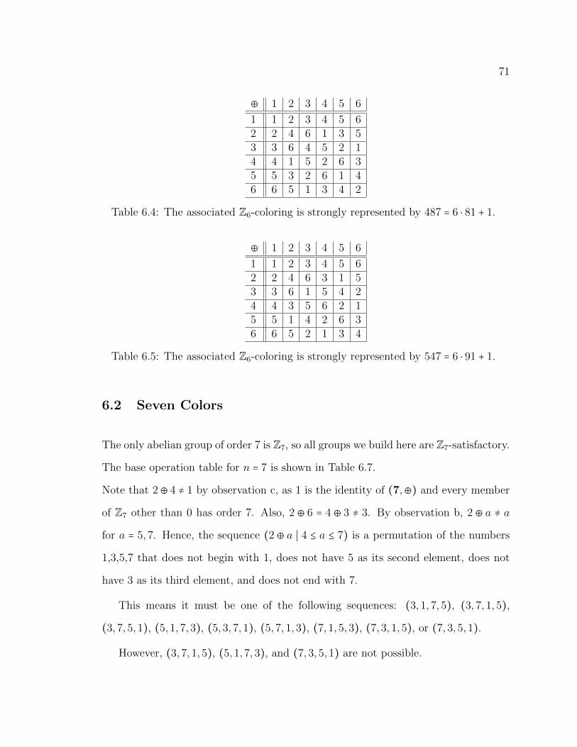
71
⊕ 1 2 3 4 5 6
1 1 2 3 4 5 62 2 4 6 1 3 53 3 6 4 5 2 14 4 1 5 2 6 35 5 3 2 6 1 46 6 5 1 3 4 2
Table 6.4: The associated Z6-coloring is strongly represented by 487 = 6 ⋅ 81 + 1.
⊕ 1 2 3 4 5 6
1 1 2 3 4 5 62 2 4 6 3 1 53 3 6 1 5 4 24 4 3 5 6 2 15 5 1 4 2 6 36 6 5 2 1 3 4
Table 6.5: The associated Z6-coloring is strongly represented by 547 = 6 ⋅ 91 + 1.
6.2 Seven Colors
The only abelian group of order 7 is Z7, so all groups we build here are Z7-satisfactory.
The base operation table for n = 7 is shown in Table 6.7.
Note that 2⊕ 4 ≠ 1 by observation c, as 1 is the identity of (7,⊕) and every member
of Z7 other than 0 has order 7. Also, 2 ⊕ 6 = 4 ⊕ 3 ≠ 3. By observation b, 2 ⊕ a ≠ a
for a = 5,7. Hence, the sequence (2 ⊕ a ∣ 4 ≤ a ≤ 7) is a permutation of the numbers
1,3,5,7 that does not begin with 1, does not have 5 as its second element, does not
have 3 as its third element, and does not end with 7.
This means it must be one of the following sequences: (3,1,7,5), (3,7,1,5),
(3,7,5,1), (5,1,7,3), (5,3,7,1), (5,7,1,3), (7,1,5,3), (7,3,1,5), or (7,3,5,1).
However, (3,7,1,5), (5,1,7,3), and (7,3,5,1) are not possible.
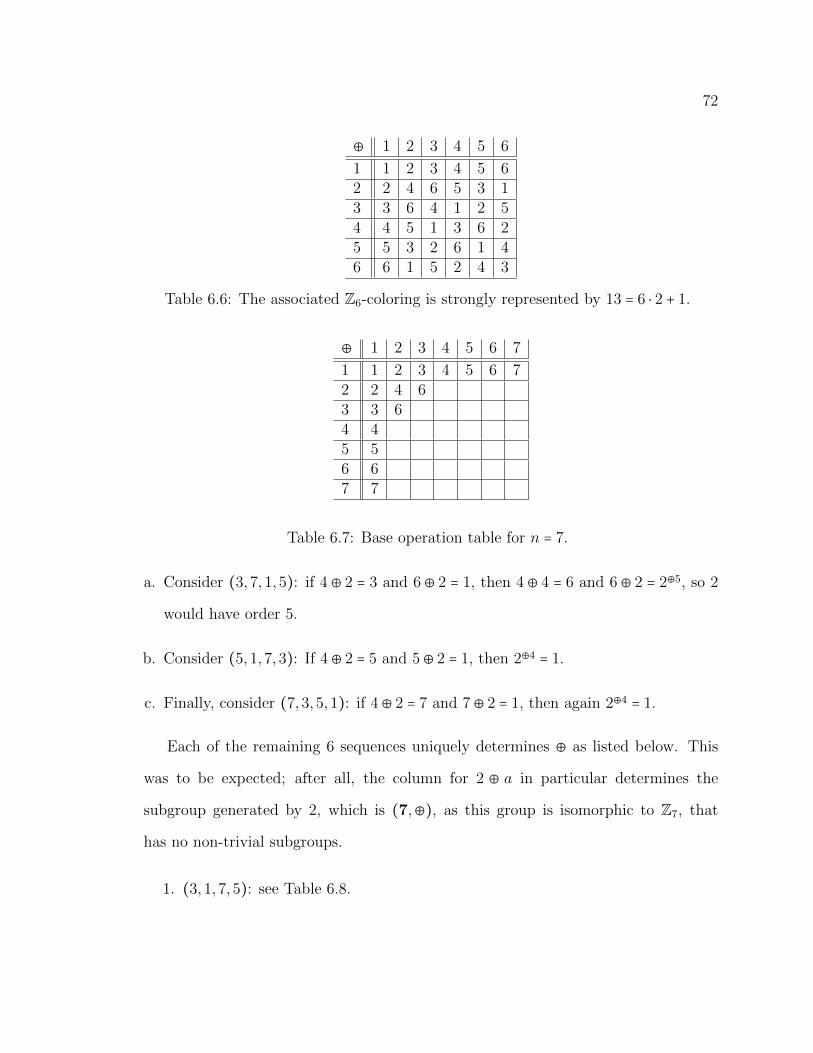
72
⊕ 1 2 3 4 5 6
1 1 2 3 4 5 62 2 4 6 5 3 13 3 6 4 1 2 54 4 5 1 3 6 25 5 3 2 6 1 46 6 1 5 2 4 3
Table 6.6: The associated Z6-coloring is strongly represented by 13 = 6 ⋅ 2 + 1.
⊕ 1 2 3 4 5 6 7
1 1 2 3 4 5 6 72 2 4 63 3 64 45 56 67 7
Table 6.7: Base operation table for n = 7.
a. Consider (3,7,1,5): if 4⊕ 2 = 3 and 6⊕ 2 = 1, then 4⊕ 4 = 6 and 6⊕ 2 = 2⊕5, so 2
would have order 5.
b. Consider (5,1,7,3): If 4⊕ 2 = 5 and 5⊕ 2 = 1, then 2⊕4 = 1.
c. Finally, consider (7,3,5,1): if 4⊕ 2 = 7 and 7⊕ 2 = 1, then again 2⊕4 = 1.
Each of the remaining 6 sequences uniquely determines ⊕ as listed below. This
was to be expected; after all, the column for 2 ⊕ a in particular determines the
subgroup generated by 2, which is (7,⊕), as this group is isomorphic to Z7, that
has no non-trivial subgroups.
1. (3,1,7,5): see Table 6.8.
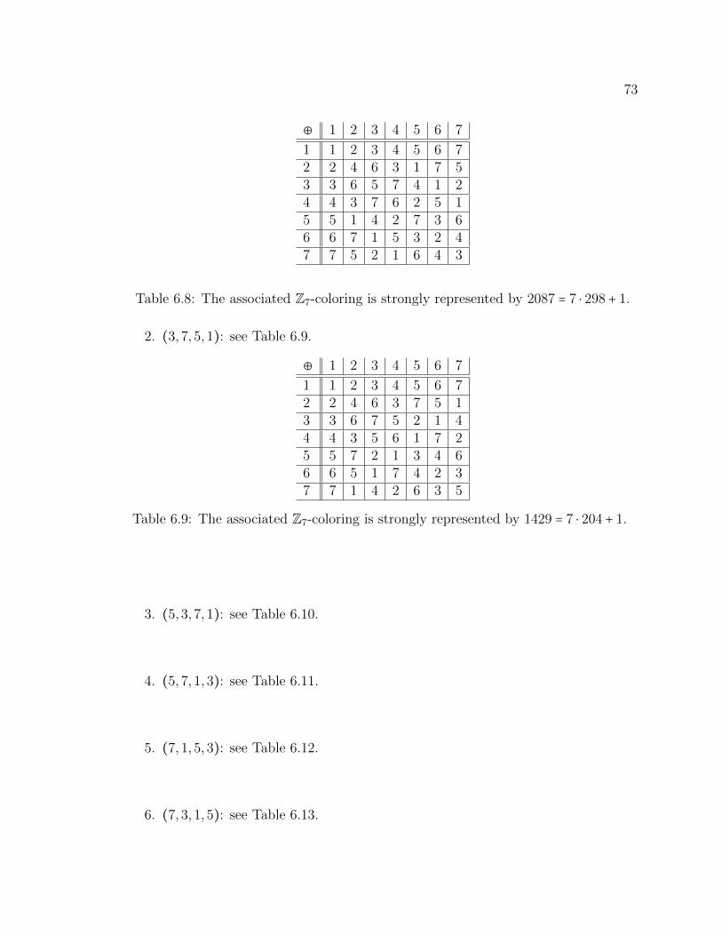
73
⊕ 1 2 3 4 5 6 7
1 1 2 3 4 5 6 72 2 4 6 3 1 7 53 3 6 5 7 4 1 24 4 3 7 6 2 5 15 5 1 4 2 7 3 66 6 7 1 5 3 2 47 7 5 2 1 6 4 3
Table 6.8: The associated Z7-coloring is strongly represented by 2087 = 7 ⋅ 298 + 1.
2. (3,7,5,1): see Table 6.9.
⊕ 1 2 3 4 5 6 7
1 1 2 3 4 5 6 72 2 4 6 3 7 5 13 3 6 7 5 2 1 44 4 3 5 6 1 7 25 5 7 2 1 3 4 66 6 5 1 7 4 2 37 7 1 4 2 6 3 5
Table 6.9: The associated Z7-coloring is strongly represented by 1429 = 7 ⋅ 204 + 1.
3. (5,3,7,1): see Table 6.10.
4. (5,7,1,3): see Table 6.11.
5. (7,1,5,3): see Table 6.12.
6. (7,3,1,5): see Table 6.13.
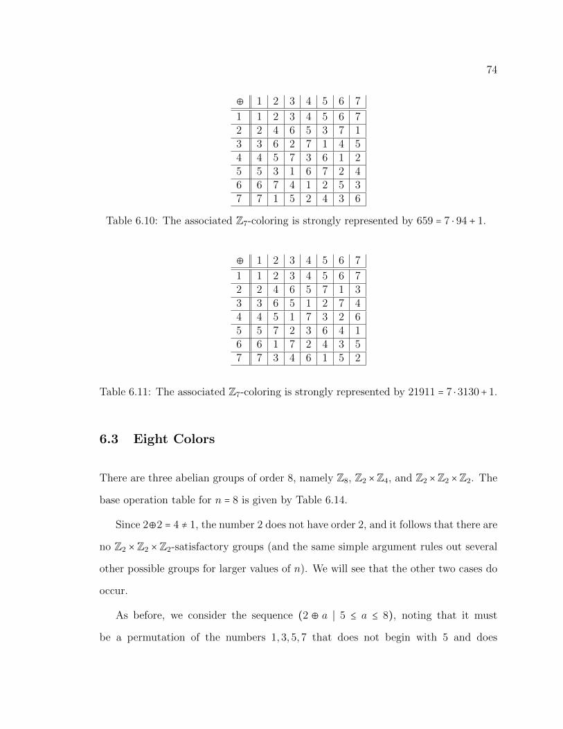
74
⊕ 1 2 3 4 5 6 7
1 1 2 3 4 5 6 72 2 4 6 5 3 7 13 3 6 2 7 1 4 54 4 5 7 3 6 1 25 5 3 1 6 7 2 46 6 7 4 1 2 5 37 7 1 5 2 4 3 6
Table 6.10: The associated Z7-coloring is strongly represented by 659 = 7 ⋅ 94 + 1.
⊕ 1 2 3 4 5 6 7
1 1 2 3 4 5 6 72 2 4 6 5 7 1 33 3 6 5 1 2 7 44 4 5 1 7 3 2 65 5 7 2 3 6 4 16 6 1 7 2 4 3 57 7 3 4 6 1 5 2
Table 6.11: The associated Z7-coloring is strongly represented by 21911 = 7 ⋅ 3130+ 1.
6.3 Eight Colors
There are three abelian groups of order 8, namely Z8, Z2 ×Z4, and Z2 ×Z2 ×Z2. The
base operation table for n = 8 is given by Table 6.14.
Since 2⊕2 = 4 ≠ 1, the number 2 does not have order 2, and it follows that there are
no Z2 ×Z2 ×Z2-satisfactory groups (and the same simple argument rules out several
other possible groups for larger values of n). We will see that the other two cases do
occur.
As before, we consider the sequence (2 ⊕ a ∣ 5 ≤ a ≤ 8), noting that it must
be a permutation of the numbers 1,3,5,7 that does not begin with 5 and does
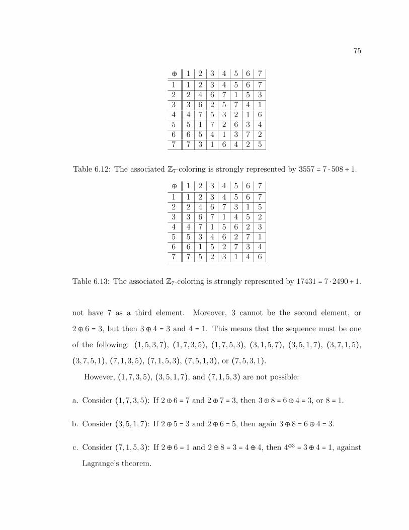
75
⊕ 1 2 3 4 5 6 7
1 1 2 3 4 5 6 72 2 4 6 7 1 5 33 3 6 2 5 7 4 14 4 7 5 3 2 1 65 5 1 7 2 6 3 46 6 5 4 1 3 7 27 7 3 1 6 4 2 5
Table 6.12: The associated Z7-coloring is strongly represented by 3557 = 7 ⋅ 508 + 1.
⊕ 1 2 3 4 5 6 7
1 1 2 3 4 5 6 72 2 4 6 7 3 1 53 3 6 7 1 4 5 24 4 7 1 5 6 2 35 5 3 4 6 2 7 16 6 1 5 2 7 3 47 7 5 2 3 1 4 6
Table 6.13: The associated Z7-coloring is strongly represented by 17431 = 7 ⋅ 2490+ 1.
not have 7 as a third element. Moreover, 3 cannot be the second element, or
2 ⊕ 6 = 3, but then 3 ⊕ 4 = 3 and 4 = 1. This means that the sequence must be one
of the following: (1,5,3,7), (1,7,3,5), (1,7,5,3), (3,1,5,7), (3,5,1,7), (3,7,1,5),
(3,7,5,1), (7,1,3,5), (7,1,5,3), (7,5,1,3), or (7,5,3,1).
However, (1,7,3,5), (3,5,1,7), and (7,1,5,3) are not possible:
a. Consider (1,7,3,5): If 2⊕ 6 = 7 and 2⊕ 7 = 3, then 3⊕ 8 = 6⊕ 4 = 3, or 8 = 1.
b. Consider (3,5,1,7): If 2⊕ 5 = 3 and 2⊕ 6 = 5, then again 3⊕ 8 = 6⊕ 4 = 3.
c. Consider (7,1,5,3): If 2⊕ 6 = 1 and 2⊕ 8 = 3 = 4⊕ 4, then 4⊕3 = 3⊕ 4 = 1, against
Lagrange’s theorem.
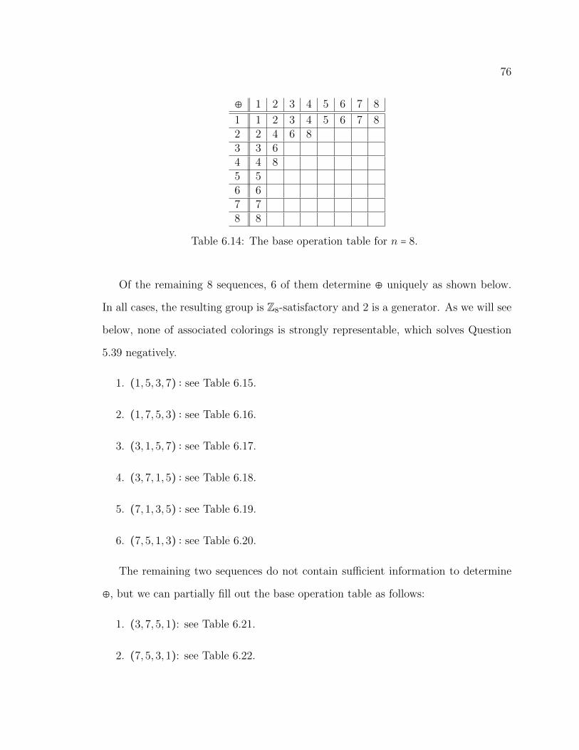
76
⊕ 1 2 3 4 5 6 7 8
1 1 2 3 4 5 6 7 82 2 4 6 83 3 64 4 85 56 67 78 8
Table 6.14: The base operation table for n = 8.
Of the remaining 8 sequences, 6 of them determine ⊕ uniquely as shown below.
In all cases, the resulting group is Z8-satisfactory and 2 is a generator. As we will see
below, none of associated colorings is strongly representable, which solves Question
5.39 negatively.
1. (1,5,3,7) ∶ see Table 6.15.
2. (1,7,5,3) ∶ see Table 6.16.
3. (3,1,5,7) ∶ see Table 6.17.
4. (3,7,1,5) ∶ see Table 6.18.
5. (7,1,3,5) ∶ see Table 6.19.
6. (7,5,1,3) ∶ see Table 6.20.
The remaining two sequences do not contain sufficient information to determine
⊕, but we can partially fill out the base operation table as follows:
1. (3,7,5,1): see Table 6.21.
2. (7,5,3,1): see Table 6.22.
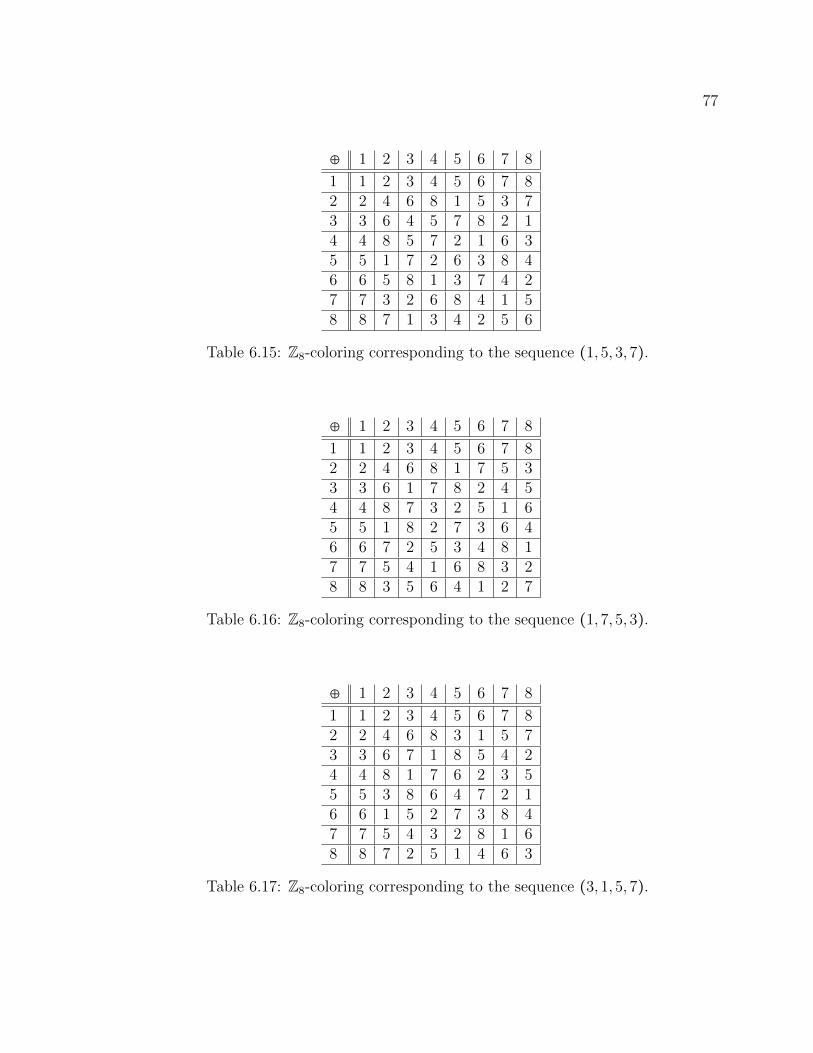
77
⊕ 1 2 3 4 5 6 7 8
1 1 2 3 4 5 6 7 82 2 4 6 8 1 5 3 73 3 6 4 5 7 8 2 14 4 8 5 7 2 1 6 35 5 1 7 2 6 3 8 46 6 5 8 1 3 7 4 27 7 3 2 6 8 4 1 58 8 7 1 3 4 2 5 6
Table 6.15: Z8-coloring corresponding to the sequence (1,5,3,7).
⊕ 1 2 3 4 5 6 7 8
1 1 2 3 4 5 6 7 82 2 4 6 8 1 7 5 33 3 6 1 7 8 2 4 54 4 8 7 3 2 5 1 65 5 1 8 2 7 3 6 46 6 7 2 5 3 4 8 17 7 5 4 1 6 8 3 28 8 3 5 6 4 1 2 7
Table 6.16: Z8-coloring corresponding to the sequence (1,7,5,3).
⊕ 1 2 3 4 5 6 7 8
1 1 2 3 4 5 6 7 82 2 4 6 8 3 1 5 73 3 6 7 1 8 5 4 24 4 8 1 7 6 2 3 55 5 3 8 6 4 7 2 16 6 1 5 2 7 3 8 47 7 5 4 3 2 8 1 68 8 7 2 5 1 4 6 3
Table 6.17: Z8-coloring corresponding to the sequence (3,1,5,7).
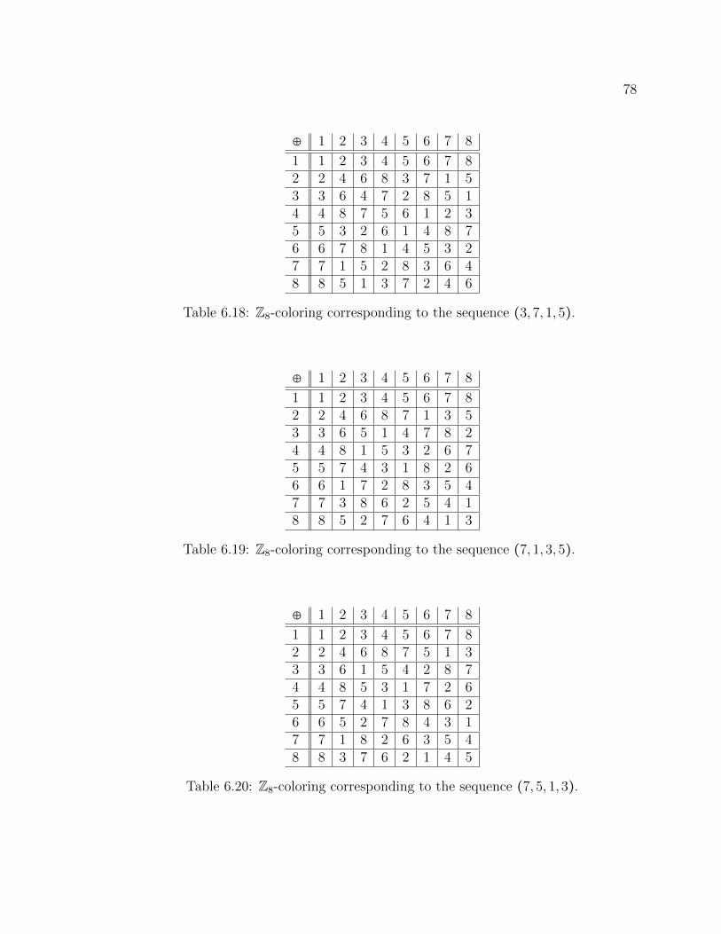
78
⊕ 1 2 3 4 5 6 7 8
1 1 2 3 4 5 6 7 82 2 4 6 8 3 7 1 53 3 6 4 7 2 8 5 14 4 8 7 5 6 1 2 35 5 3 2 6 1 4 8 76 6 7 8 1 4 5 3 27 7 1 5 2 8 3 6 48 8 5 1 3 7 2 4 6
Table 6.18: Z8-coloring corresponding to the sequence (3,7,1,5).
⊕ 1 2 3 4 5 6 7 8
1 1 2 3 4 5 6 7 82 2 4 6 8 7 1 3 53 3 6 5 1 4 7 8 24 4 8 1 5 3 2 6 75 5 7 4 3 1 8 2 66 6 1 7 2 8 3 5 47 7 3 8 6 2 5 4 18 8 5 2 7 6 4 1 3
Table 6.19: Z8-coloring corresponding to the sequence (7,1,3,5).
⊕ 1 2 3 4 5 6 7 8
1 1 2 3 4 5 6 7 82 2 4 6 8 7 5 1 33 3 6 1 5 4 2 8 74 4 8 5 3 1 7 2 65 5 7 4 1 3 8 6 26 6 5 2 7 8 4 3 17 7 1 8 2 6 3 5 48 8 3 7 6 2 1 4 5
Table 6.20: Z8-coloring corresponding to the sequence (7,5,1,3).
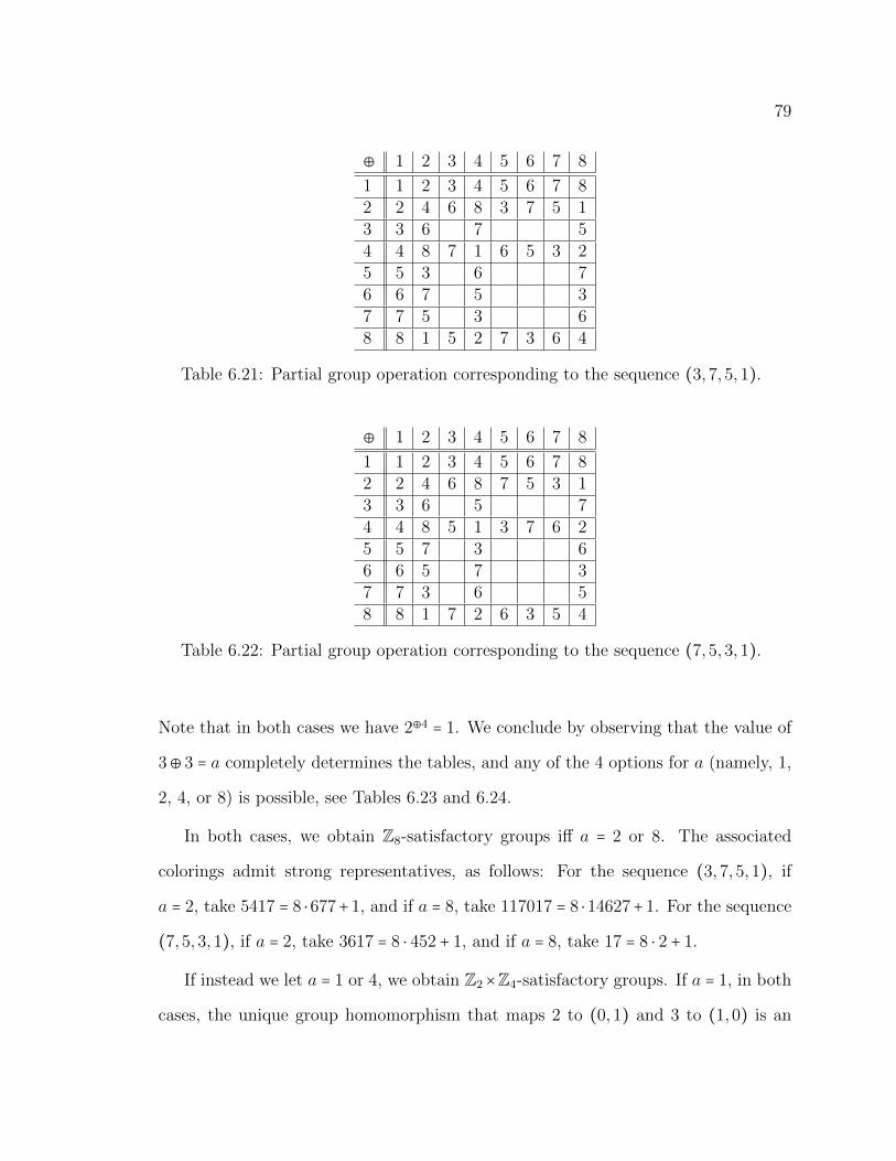
79
⊕ 1 2 3 4 5 6 7 8
1 1 2 3 4 5 6 7 82 2 4 6 8 3 7 5 13 3 6 7 54 4 8 7 1 6 5 3 25 5 3 6 76 6 7 5 37 7 5 3 68 8 1 5 2 7 3 6 4
Table 6.21: Partial group operation corresponding to the sequence (3,7,5,1).
⊕ 1 2 3 4 5 6 7 8
1 1 2 3 4 5 6 7 82 2 4 6 8 7 5 3 13 3 6 5 74 4 8 5 1 3 7 6 25 5 7 3 66 6 5 7 37 7 3 6 58 8 1 7 2 6 3 5 4
Table 6.22: Partial group operation corresponding to the sequence (7,5,3,1).
Note that in both cases we have 2⊕4 = 1. We conclude by observing that the value of
3⊕ 3 = a completely determines the tables, and any of the 4 options for a (namely, 1,
2, 4, or 8) is possible, see Tables 6.23 and 6.24.
In both cases, we obtain Z8-satisfactory groups iff a = 2 or 8. The associated
colorings admit strong representatives, as follows: For the sequence (3,7,5,1), if
a = 2, take 5417 = 8 ⋅ 677+ 1, and if a = 8, take 117017 = 8 ⋅ 14627+ 1. For the sequence
(7,5,3,1), if a = 2, take 3617 = 8 ⋅ 452 + 1, and if a = 8, take 17 = 8 ⋅ 2 + 1.
If instead we let a = 1 or 4, we obtain Z2×Z4-satisfactory groups. If a = 1, in both
cases, the unique group homomorphism that maps 2 to (0,1) and 3 to (1,0) is an
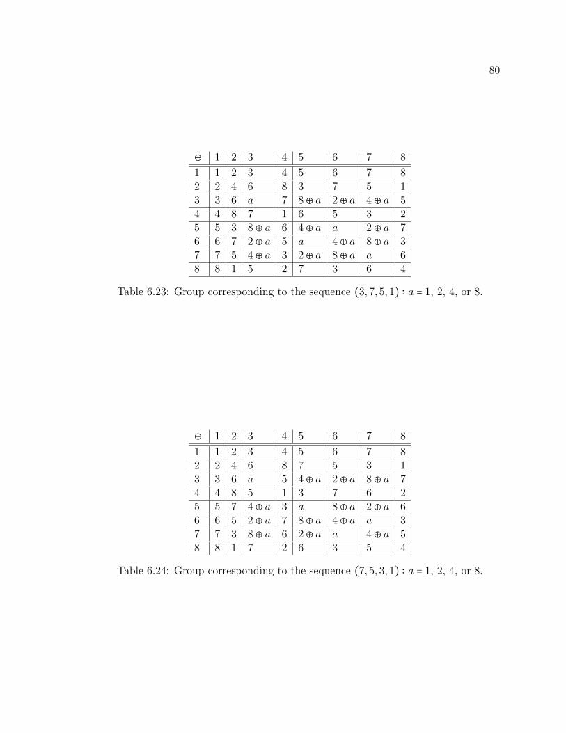
80
⊕ 1 2 3 4 5 6 7 8
1 1 2 3 4 5 6 7 82 2 4 6 8 3 7 5 13 3 6 a 7 8⊕ a 2⊕ a 4⊕ a 54 4 8 7 1 6 5 3 25 5 3 8⊕ a 6 4⊕ a a 2⊕ a 76 6 7 2⊕ a 5 a 4⊕ a 8⊕ a 37 7 5 4⊕ a 3 2⊕ a 8⊕ a a 68 8 1 5 2 7 3 6 4
Table 6.23: Group corresponding to the sequence (3,7,5,1) ∶ a = 1, 2, 4, or 8.
⊕ 1 2 3 4 5 6 7 8
1 1 2 3 4 5 6 7 82 2 4 6 8 7 5 3 13 3 6 a 5 4⊕ a 2⊕ a 8⊕ a 74 4 8 5 1 3 7 6 25 5 7 4⊕ a 3 a 8⊕ a 2⊕ a 66 6 5 2⊕ a 7 8⊕ a 4⊕ a a 37 7 3 8⊕ a 6 2⊕ a a 4⊕ a 58 8 1 7 2 6 3 5 4
Table 6.24: Group corresponding to the sequence (7,5,3,1) ∶ a = 1, 2, 4, or 8.
81
isomorphism between (8,⊕) and Z2 ×Z4. If a = 4 and the sequence is (3,7,5,1), the
corresponding isomorphism is obtained by considering the homomorphism that maps
2 to (0,1) and 5 to (1,0). If a = 4 and the sequence is (7,5,3,1), consider instead the
homomorphism that maps 2 to (0,1) and 7 to (1,0).
Finally, we argue that the colorings associated with the first six Z8-satisfactory
groups we listed are not strongly representable. For this, simply note that if they
were, any strong representative must be of the form p = 8k + 1, so (by Theorem 1.10)
24k ≡ 1 (mod p).
But 24k = (24)k, so the corresponding coloring c must satisfy c(2⊕8) = c(24) = 1 = c(1),
that is, we must have 2 ⊕ 8 = 1. For a high–level explanation of why some of these
Z8-colorings are strongly representable while others are not, see Theorem 7.18.
82
CHAPTER 7
FINAL REMARKS
7.1 A Conjecture of R.L. Graham
Theorem 7.1. (Balasubramanian–Soundararajan, 1996)
Let n ≥ 1, and 0 < a1 < a2 < . . . < an be integers. Then maxi,j
{ ai(ai, aj)
} ≥ n.
Theorem 7.1 originated as a conjecture of R.L. Graham of 1970, see [?]. An
affirmative answer was published in 1996 by Balasubramanian and Soundararajan,
see [7]. Interestingly an affirmative answer to the question of whether there are
satisfactory colorings for all n implies Theorem 7.1.
Theorem 7.2. Conjecture 5.5 implies Theorem 7.1. In fact, if there are satisfactory
colorings with m − 1 colors, then Theorem 7.1 holds for n =m.
Proof. Suppose that there exists some m and a set B = {b1, . . . , bm} with 0 < b1 < . . . <
bm such that maxi,j
{ bi(bi, bj)
} < m. Suppose i ≠ j and let M = (bi, bj). Let biM = ai and
bjM = aj. By our hypothesis, we have that ai < m, aj < m, and ai ≠ aj. Since bi = aiM,
bj = ajM, in any satisfactory coloring with at least m− 1 colors, we must have that bi
is colored differently than bj. But ∣B∣ =m so we need, at least, m colors.
The proof of Theorem 7.1 in [7] requires careful analytic estimates of average
values of number theoretic functions associated with the distribution of primes. This
83
may say something about the inherent difficulty of Conjecture 5.5. Using purely
elementary arguments, Velez [8] established a particular case of Theorem 7.1. We
present the argument in hope that a suitable adaptation may establish Conjecture
5.5 for n colors, when n = p is a prime.
The remainder of the section follows [8] closely.
Theorem 7.3. (Velez, 1977) [8]
Theorem 7.1 is true for n = p + 1, with p prime.
Before proving this theorem, we begin with some remarks and preliminary results.
1. If we multiply a sequence by a constant, we obtain the same set of ratios, so we
may assume (a1, a2, . . . , an) = 1.
2. Given a sequence Q = {a1 < a2 < ⋯ < an}, let A = lcm(a1, a2, . . . , an) and form
Q−1 = { Aan
< A
an−1< ⋯ < A
a1}.
It is easily seen that Q and Q−1 yield the same set of ratios.
Define Mn = lcm(1,2, . . . , n) and b(n)i = Mn
n−i+1 , so Mn
n < Mn
n−1 < ⋯ < Mn
2 < Mn
1 is the
pseudo-inverse of n. We are now ready to begin the proof.
Definition 7.4. Given a sequence a1 < a2 < . . . < an, call it a standard sequence if it
is a multiple of n or of {b(n)1 < b(n)2 < . . . < b(n)n }. That is, either
ai = ki for all i,
or
ai = kb(n)i for all i.
84
In fact, Balasubramanian–Soundararajan [7] established a strong form of Gra-
ham’s conjecture, where they determine the circumstances under which equality holds:
Theorem 7.5. (Balasubramanian–Soundararajan, 1996) [7]
Assume (a1, a2, . . . , an) = 1 and maxi,j
{ ai(ai, aj)
} = n. Then, the sequence is a standard
sequence except for n = 4, where we have the additional sequence {2,3,4,6}.
Following Velez [8], we prove in Theorem 7.7 that Theorem 7.5 is indeed a
strengthening of Theorem 7.1. We now begin the argument towards Theorem 7.3.
We do not assume either Theorem 7.1 or 7.5.
Theorem 7.6. Let q = {a1 < a2 < . . . < an} be a standard sequence and b be any
integer such that b ≠ ai for any i and (a1, a2, . . . , an, b) = 1. Form the new sequence
Q′ = {a1 < a2 < . . . < an, b} (where b is inserted in the appropriate place). Then, if Q′
is not a standard sequence, we have
maxi,j
{ ai(ai, aj)
,b
(ai, b),
ai(ai, b)
} > n + 1,
except possibly when n = 4.
Proof. Note that (a1, a2, . . . , an, b) = 1 is not a restriction. To see this, assume ai =
k′b(n)i . Let a = lcm(a1, a2, . . . , an, b) and form the new sequence
{ a
an< a
an−1< . . . < a
a1,a
b}.
Hence, we have the new sequence
Q′ = {k < 2k < . . . < nk, b′} with (b′, k) = 1.
85
We will prove the theorem for this sequence.
Assume Q′ is not a standard sequence. If k = 1, then b′ ≠ n + 1, since Q′ is not a
standard sequence. Hence, b′ > n+1, but then b′(k,b′) = b′ > n+1. Hence, we may assume
that k > 1. If b′ > n + 1, then b′(k,b′) = b′ > n + 1. If b′ = n + 1, then kn
(kn,b′) = kn > n + 1.
If b′ = n, then k(n−1)(k(n−1),b′) = k(n − 1) > n + 1 for k > 2 or n > 3. If k = 2 and n = 3,
then 2(3 − 1) = 3 + 1 and this gives the sequence {2 < 4 < 6, b′ = 3}. If b′ = n − 1, then
kn(b′,kn) = kn > n = 1. Hence, we may assume that b′ < n − 1, so b′ + 1 < n and k(b′ + 1)
appears somewhere in the sequence Q′ and
k(b′ + 1)(k(b′ + 1), b′) = k(b′ + 1).
If k(b′ + 1) > n + 1, then we are done. If not, then kb′ + 1 < kb′ + k ≤ n + 1. Define l by
k(kl+1b′ + 1) > n = 1,
k(klb′ + 1) ≤ n + 1.
Then, l ≥ 0 and we have that kl+1b′+1 < kl+1b′+k ≤ n+1, so kl+1b′+1 ≤ n; k(kl+1b′+1)
appears somewhere in the sequence Q′, and
k(kl+1b′ + 1)(k(kl+1b′ + 1), b′) = k(kl+1b′ + 1) > n + 1.
Theorem 7.7. Theorem 7.5 implies Theorem 7.1. In fact, if Theorems 7.1 and 7.5
hold for n, then Theorem 7.1 holds for n + 1.
Proof. We proceed by induction on n. Assume that Theorem 7.1 is true for n and
86
consider
0 < a1 < . . . < an < an+1.
Then, by induction, we know that
max1≤i,j≤n
{ ai(ai, aj)
} ≥ n.
If max1≤i,j≤n
{ ai(ai, aj)
} > n, then
max1≤i,j≤n+1
{ ai(ai, aj)
} ≥ n + 1.
Hence, we may assume that
max1≤i,j≤n
{ ai(ai, aj)
} = n.
By Theorem 7.5, the sequence is standard, i.e., a1 < a2 < . . . < an is a standard
sequence. Now by Theorem 7.6 we have
max1≤i,j≤n+1
{ ai(ai, aj)
} ≥ n + 1.
Theorem 7.8. (Szemeredi) [8]
Theorem 7.1 is true for n = p, where p is prime.
Proof. This follows immediately from Theorem 7.2, since Conjecture 5.5 holds with
p − 1 colors, by Theorem 5.1.
87
Lemma 7.9. If (ai, a2, . . . , an) = 1, maxi,j
{ ai(ai, aj)
} ≤ n and p is a prime with p∣ai, for
some i, then p ≤ n.
Proof. Since (ai, a2, . . . , an) = 1 and p∣ai, there exists an aj such that p ∤ aj. Hence,
ai(ai,aj)
≥ p. However, by our hypothesis maxi,j
{ ai(ai, aj)
} ≤ n, hence we have p ≤ n.
Lemma 7.10. If (a1, a2, . . . , an) = 1 and maxi,j
{ ai(ai, aj)
} ≤ n, then ai∣Mn for all i.
Proof. Let Mn = pl11 ⋯plss and assume pli+1i ∣ak. Then, there exists aj such that (aj, pi) =
1. Hence,
pli+1i ∣ ak(aj, ak)
.
But this says that the ratio is larger than n. We now see that if the maximum of the
ratios is ≤ n, then each element of the sequence divides Mn.
Lemma 7.11. If a1 = b(n)1 = Mn
n and maxi,j
{ ai(ai, aj)
} ≤ n with (a1, . . . , an) = 1, then
ai = b(n)i for all i.
Proof. We have a1 = Mn
n , ak =jka1ik, (ik, jk) = 1, ik ≤ jk ≤ n. Assume (jk, n) = d ≠ jk.
Then, there exists a prime p = p1 such that p1∣jk, p1 ∤ n. Thus, since pl11 ∣a1 and
(ik, jk) = 1, we have pl1+11 ∣ak, which contradicts Lemma 7.10. Hence, jk∣n so that
ak =na1dk
, 1 ≤ dk ≤ n.
But the ak are increasing and there are exactly n of them; hence, this says d1 = n, d2 =
n − 1, . . . , dn = 1, i.e.,
ak =na1
n − k + 1= Mn
n − k + 1.
88
Corollary 7.12. If (a1, . . . , an) = 1 and maxi,j
{ ai(ai, aj)
} ≤ n, then ai ≤ b(n)i , for all i.
Proof. Since maxi,j
{ ai(ai, aj)
} ≤ n, we have that ai = Mn
ci, where c1 > c2 > . . . > cn. If
ai > b(n)i , then Mn
ci> Mn
n−i+1 , so n− i+1 > ci. So we have that n− i+1 > ci > ci+1 > . . . > cn.
Hence,
{ci, ci+1, . . . , cn} ⊂ {1,2, . . . , n − i}.
But ∣{ci, ci+1, . . . , cn}∣ = n− i+1 > n− i = ∣{1,2, . . . , n− i}∣, and we have a contradiction.
Theorem 7.13. Theorem 7.5 is true for n = p, p a prime.
Proof. We may assume that (a1, . . . , an) = 1. Since ai(ai,aj)
≤ p, we have that ai ≤ paj.
If ai ≠ paj, for all i, j, consider a′i = ai
(ai,p). Then, ∣{a′1, . . . , a
′p}∣ = p. Furthermore, since
p2 ∤ Mp, where Mp is the least common multiple of p, we have that(a′i, p) = 1, so
maxi,j
{ ai(ai, aj)
} < p, which contradicts Theorem 7.8. Hence, for some i, j, we must
have ai = paj. But this implies that i = 1, j = p and ap = pa1. Furthermore, since
p2 ∤Mp, p ∤ a1. If p∣ai for all i > 1, then ai = pa1ci, with c1 = p > c2 > . . . > cp = 1. Hence,
ai = b(n)i and a1 < . . . < an is a standard sequence. Assume that (ai, p) = 1 for some
i > 1. Then, ai = k1a1k2, (k1, k2) = 1,k2∣a1, k2 < k1 < p. Then (ap, ai) = (pa1, k1a1k2
) = a1k2, so
ap(ai,ap)
= pk2 ≤ p, which implies k2 = 1. So we have that if (ai, p) = 1, then ai = kia1.
If aj = pa1c , (c, p) = 1, then (ai, aj) = (pa1c ,
kica1c ) = a1
c . Hence, ai(ai,aj)
= kia1a1c
= kic ≤ p,
so ki < pc , since (kic, p) = 1. Hence, kia1 < pa1
c , so ai < aj. That is, the sequence
a1 < . . . < ap takes the form
a1 < a1k1 < . . . < a1kl <pa1c1
< . . . < pa1cr
< pa11. (7.1)
89
If kl > p2 , then p
c1> kl > p
2 , so c1 < 2, that is c1 = 1 and (7.1) becomes
a1 < 2a1 < 3a1 < . . . < (p − 1)a1 < pa1, (7.2)
so a1 = 1, since (a1, . . . , ap) = 1, and (7.2) is a standard sequence. Assume that kl < p2 ,
that is, ∣{ai ∶ (ai, p) = 1}∣ < p2 . Since there is at least one ai, i > 1, such that (ai, p) = 1,
we have that pc1> kl ≥ 2, so c1 < p
2 , that is, the ci must assume fewer than p2 values.
Hence, ∣{ai ∶ p∣ai}∣ < p2 . But
{a1, a2, . . . , ap} = {ai ∶ p∣ai} ∪ {ai ∶ (ai, p) = 1}
and this implies that
∣{a1, a2, . . . , ap}∣ = p <p
2+ p
2< p,
so p < p. Hence, kl ≰ p2 .
Corollary 7.14. Theorem 7.1 is true for n = p + 1, p a prime.
Proof. Since Theorems 7.1 and 7.7 are true for n = p, p a prime, Theorem 7.6 readily
gives us the desired result.
In our attempts to provide proof of the existence of partial homomorphisms of
arbitrary order, we turned to trying to find a way in which a given partial homomor-
phism can be extended or truncated. It is in this light that the result of Velez may
prove useful.
Question 7.15. Given any prime p, is there at least one partial homomorphism of
order p − 1 that can be extended to produce a partial homomorphism of order p?1
1The answer is no in general. See Section 7.2 and Appendix C.
90
A natural attempt towards solving Question 7.15 affirmatively would be to show
that there is a partial homomorphism h ∶ p − 1→ Zp−1 such that, defining h(p) = p−1,
the resulting extension is a partial homomorphism. This would be the case if we
could ensure that there is at least one such h that does not require any “carrying,”
i.e., such that if a, b, ab ∈ p − 1, then h(a) + h(b) = h(ab) in Z, not just in Zp−1.
7.2 A Late Conclusion
Four days after the defense of this thesis, Zack Teitler informed us of a series of
articles that allow us to answer the question of whether multiplicative colorings exist
for all n. The motivation for the research done in the articles was the conjecture
of Graham, which resulted in the Balasubramanian–Soundararajan Theorem of the
previous section.
Without further ado, let us first state the following theorem concerning the exis-
tence of multiplicative colorings.
Theorem 7.16. There exist n ∈ Z+ for which no multiplicative coloring exists. In
fact, the smallest such n is n = 195.
This refutes what seemed to be the prevailing opinion, that a careful probabilistic
argument would prove the existence of multiplicative colorings for all n, see for
example Greg Kuperberg’s suggestion in [2].
The proof follows from the work initiated by Rodney Forcade, Jack Lamoreaux,
and Andrew Pollington when they posed the following question in 1986, see [18].
Question 7.17. Is it possible, changing only those products that exceed n, to make
the set n into a multiplicative group?
91
Note that, in our terminology, the question corresponds to asking whether G-
satisfactory groups exist for all values of n. In the article, they conjecture that the
answer to Question 7.17 is affirmative. In their discussion, they also ask (in different
terms) whether strong representatives exist for all values of n.
In 1990, perhaps surprisingly, Forcade and Pollington answered Question 7.17
negatively, see [19]. To do so they employed an exhaustive search algorithm that, in
the case of n = 195, did not produce a G-satisfactory group.
We refer to those values of n for which no G-satisfactory group exist as groupless
n. We included in Appendix C a list of all groupless n ≤ 500.
Additionally, the work of Simon Blackburn and James McKee, in [21], is particu-
larly relevant. In their paper, partial Zn-homomorphisms are referred to as “bijective
logarithms of length n,” or, simply, “logarithms of length n”. Several references where
they are studied are provided in their Section 5.1. Using our terminology, we now
state their Theorem 5.1. For proof, see [20].2
Theorem 7.18. (Kummer, Mills)
Let h be a partial Zn-homomorphism.
(a) If n is odd, then the associated Zn-coloring is strongly representable.
(b) If n ≡ 2 mod 4, then the associated Zn-coloring is strongly representable iff h(m)
is even whenever m divides n and m ≡ 1 (mod 4).
(c) If n ≡ 0 mod 4, then the associated Zn-coloring is strongly representable iff h(m)
is even whenever m divides n/4.
2It is noteworthy to mention that the argument makes essential use of Chebotarev’s densitytheorem, a subtle generalization of Dirichlet’s theorem.
92
(d) If there is one strong representative of order n, then there are in fact infinitely
many.
Also, in Blackburn–McKee, [21] Section 5.2, Domotor’s coloring question, Ques-
tion 4.1 of this thesis, is considered (independently), in the language of tilings of
powers of Z. In [21] Section 9.2, they discuss the number of partial homomorphisms
for a given n and present a table of values of n ≤ 300 that do not admit partial
Zn-homomorphisms.3 Blackburn-McKee [21] suggest, based on numerical evidence,
that if n is large enough, then there is a partial Zn-homomorphism iff n + 1 or n2 + 1
is prime. Perhaps, in fact, for n large enough, there is a G-satisfactory group (even
without the restriction of G being abelian) iff the same restriction on n holds: n + 1
or n2 + 1 is prime so, in fact, there is a Zn-satisfactory group.4
In closing, we mention the following: Although it is known that multiplicative col-
orings do not exist for all values of n, the question of whether satisfactory colorings ex-
ist for all values of n remains open. As evidenced by Theorem 5.40, non-multiplicative
satisfactory colorings do in fact exist. Thus, if one is to make progress in solving the
problem, then it will require a better understanding of non-multiplicative colorings.
Perhaps a good place to start this analysis would be the case of n = 195.
3The table they present coincides with our Table C.1.4See Remark 5.42.
93
REFERENCES
[1] Melvin B. Nathanson. Elementary Methods in Number Theory. Springer-Verlag,New York, 2000.
[2] Palvolgyi Domotor. http://mathoverflow.net/questions/26358/can-we-color-z-with-n-colors-such-that-a-2a-na-all-have-different-colors
[3] KoMaL. http://www.komal.hu/verseny/feladat.cgi?a=honaph=201004t=matl=en
[4] Alexander Soifer. The Mathematical Coloring Book, Mathematics of Coloringand the Colorful Life of Its Creators. Springer, New York, 2009.
[5] Terence Tao and Van Vu. Additive Combinatorics. Cambridge University Press,Cambridge, 2006.
[6] Eric W. Weisstein. “Graph Coloring.” From MathWorld–A Wolfram Web Re-source. http://mathworld.wolfram.com/GraphColoring.html
[7] Ramachandran Balasubramanian and Kannan Soundararajan. On a conjectureof R. L. Graham. Acta Arithmetica, LXXV.1 (1996), pp. 1–38.
[8] William Yslas Velez. Some Remarks On a Number Theoretic Problem of Graham.Acta Arithmetica, XXXII (1977), pp. 232–238.
[9] Andres E. Caicedo. Regressive functions on pairs. European Journal of Combi-natorics (2009), doi:10.1016/j.ejc.2009.07.010
[10] Ronald Graham, Bruce Rothschild, Joel Spencer. Ramsey Theory, second edi-tion. John Wiley and sons, New York, N.Y., 1990.
[11] Andras Hajnal. Infinitary combinatorics, in Handbook of Combinatorics, Vol. II,Ronald Graham, Martin Grotschel, Laszlo Lovasz, eds., Elsevier, The MIT Press,1995, 2085–2116.
[12] Markus Meringer, Eric W. Weisstein. “Regular Graph.” From MathWorld–AWolfram Web Resource. http://mathworld.wolfram.com/RegularGraph.html
[13] Kenneth Falconer. The realization of distances in measurable subsets coveringRn. Journal of Combinatorial Theory Series A, vol 31 (2), (1981), 184–189.
94
[14] Dan Pritkin. All unit-distance graphs of order 6197 are 6-colorable. Journal ofCombinatorial Theory Series B, vol 73 (2) (1998), 159–163.
[15] Andres E. Caicedo (mathoverflow.net/users/6085), Fifth powers modulo a prime,http://mathoverflow.net/questions/78270 (version: 2011-10-16).
[16] Lawrence C. Washington. Introduction to Cyclotomic Fields, second edition.Springer-Verlag, New York, 1997.
[17] Kustaa Inkeri. The Real Roots of Bernoulli Polynomials. Ann. Univ. Turku. Ser.A I 37 1959 20.
[18] Rodney Forcade, Jack Lomoreaux and Andrew Pollington. A Group of TwoProblems in Groups. The American Mathematical Monthly, vol 93, No 2 (Feb.,1986), pp. 119-121.
[19] Rodney Forcade, Andrew Pollington. What is special about 195? Groups, nthpower maps and a problem of Graham. Proceddings of the First Conference ofthe Canadian Number Theory Association, Banff, 1988, R.A. Mollin, ed., Walterde Gruyter, Belin, 1990.
[20] W.H. Mills. Characters with preassigned values. Canad. J. Math., 15 (1963), pp.169–171.
[21] Simon Blackburn, James McKee. Constructing k-radius Sequences. (Mathemat-ics of computation, to appear.)
[22] Bronislaw Knaster. Un theoreme sur les fonctions d’ensenmbles. Ann. Soc. Polon.Math, vol 6 (1928), pp. 133–134.
[23] Alfred Tarski. A lattice-theoretical fixpoint theorem and its applications. PacificJournal of Mathematics, vol 5, No 2 (1955), pp. 285–309.
[24] Karen Chandler. Groups formed by redefining multiplication. Canad. Math. Bull.vol 31, No 4 (1988), pp. 419–423.
[25] Ronald Graham. Advanced Problem 5749. The American Mathematical Monthly,vol 77, No 7 (Aug. - Sep., 1970), p. 775.
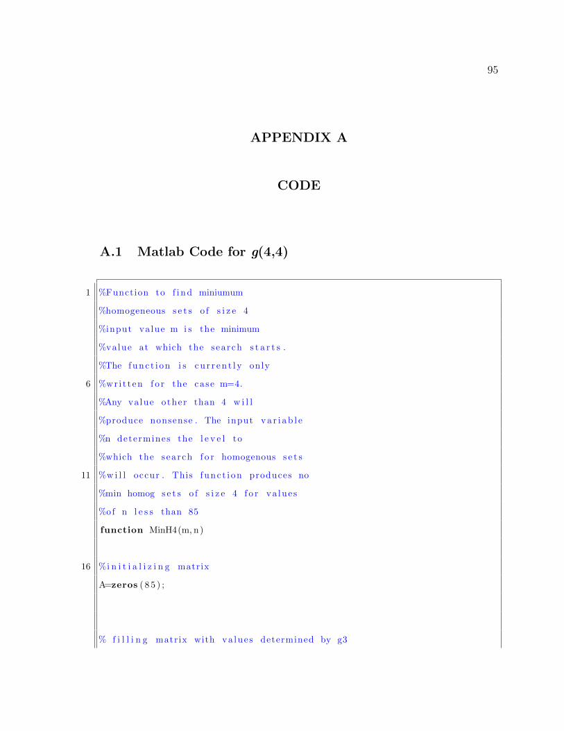
95
APPENDIX A
CODE
A.1 Matlab Code for g(4,4)
1 %Function to f i n d miniumum
%homogeneous s e t s o f s i z e 4
%input value m i s the minimum
%value at which the search s t a r t s .
%The func t i on i s c u r r e n t l y only
6 %wr i t t en f o r the case m=4.
%Any value other than 4 w i l l
%produce nonsense . The input v a r i a b l e
%n determines the l e v e l to
%which the search f o r homogenous s e t s
11 %w i l l occur . This func t i on produces no
%min homog s e t s o f s i z e 4 f o r va lue s
%o f n l e s s than 85
function MinH4(m, n)
16 %i n i t i a l i z i n g matrix
A=zeros ( 8 5 ) ;
% f i l l i n g matrix with va lue s determined by g3
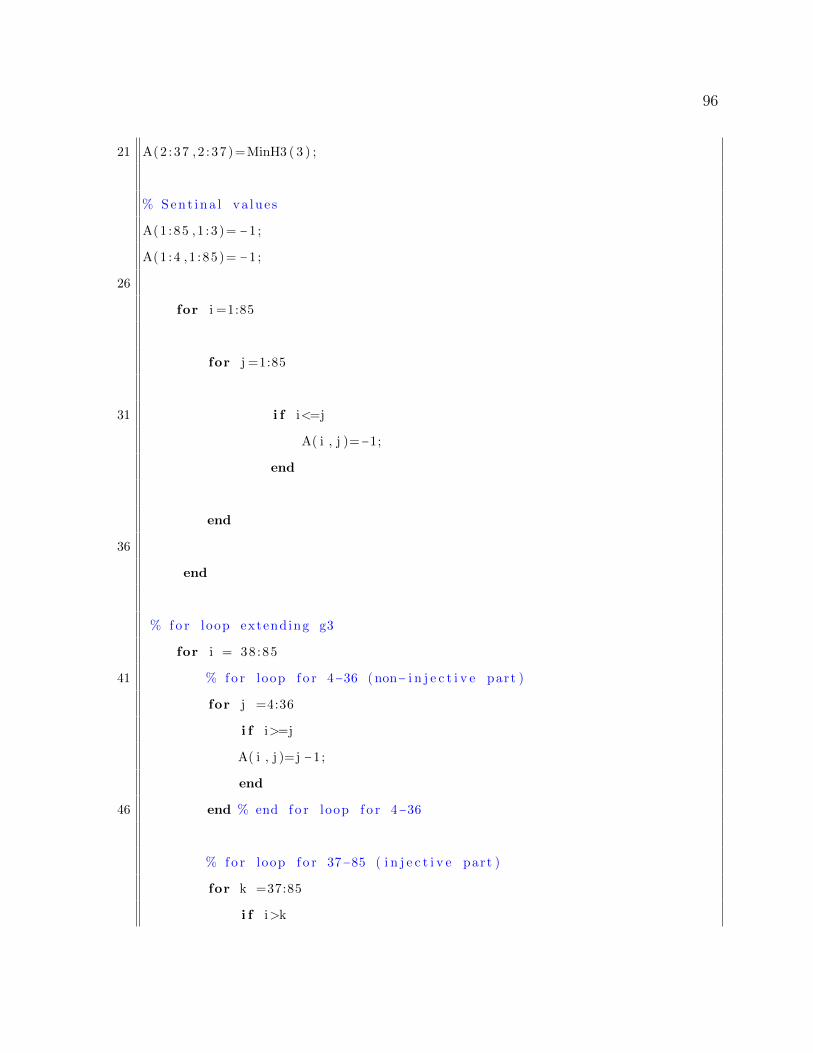
96
21 A(2 :37 ,2 : 37 )=MinH3 ( 3 ) ;
% Sent ina l va lue s
A(1 :85 ,1 :3 )= −1 ;
A(1 :4 ,1 :85)= −1 ;
26
for i =1:85
for j =1:85
31 i f i<=j
A( i , j )=−1;
end
end
36
end
% f o r loop extending g3
for i = 38 :85
41 % f o r loop f o r 4−36 ( non− i n j e c t i v e part )
for j =4:36
i f i>=j
A( i , j )=j −1;
end
46 end % end f o r loop f o r 4−36
% f o r loop f o r 37−85 ( i n j e c t i v e part )
for k =37:85
i f i>k
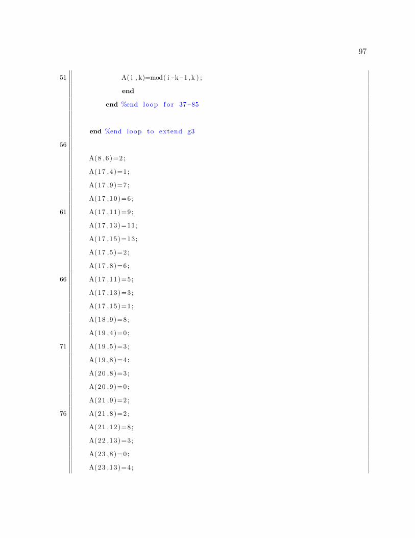
97
51 A( i , k)=mod( i −k−1 ,k ) ;
end
end %end loop f o r 37−85
end %end loop to extend g3
56
A(8 ,6)=2;
A(17 ,4)=1;
A(17 ,9)=7;
A(17 ,10)=6;
61 A(17 ,11)=9;
A(17 ,13)=11;
A(17 ,15)=13;
A(17 ,5)=2;
A(17 ,8)=6;
66 A(17 ,11)=5;
A(17 ,13)=3;
A(17 ,15)=1;
A(18 ,9)=8;
A(19 ,4)=0;
71 A(19 ,5)=3;
A(19 ,8)=4;
A(20 ,8)=3;
A(20 ,9)=0;
A(21 ,9)=2;
76 A(21 ,8)=2;
A(21 ,12)=8;
A(22 ,13)=3;
A(23 ,8)=0;
A(23 ,13)=4;
98
81 A(24 ,13)=5;
A(25 ,13)=6;
A(26 ,13)=7;
A(27 ,13)=8;
A(28 ,13)=9;
86 A(29 ,13)=10;
A(32 ,12)=0;
A(33 ,12)=1;
A(34 ,12)=2;
A(35 ,12)=3;
91 A(36 ,12)=4;
A(37 ,12)=5;
A(38 ,4)=2;
A(38 ,20)=17;
A(38 ,5)=1;
96 A(38 ,6)=0;
A(38 ,7)=0;
A(38 ,8)=2;
A(38 ,9)=1;
A(38 ,10)=6;
101 A(38 ,12)=6;
A(38 ,14)=3;
A(38 ,15)=3;
A(38 ,16)=3;
A(38 ,17)=3;
106 A(38 ,19)=5;
A(39 ,4)=2;
A(39 ,5)=0;
A(39 ,6)=3;
A(39 ,7)=4;
99
111 A(39 ,8)=5;
A(39 ,9)=2;
A(39 ,11)=6;
A(39 ,13)=4;
A(39 ,14)=4;
116 A(39 ,15)=4;
A(39 ,16)=4;
A(39 ,17)=4;
A(39 ,19)=6;
A(39 ,20)=18;
121 A(39 ,21)=16;
A(40 ,4)=2;
A(40 ,5)=1;
A(40 ,6)=2;
A(40 ,7)=3;
126 A(40 ,8)=6;
A(40 ,9)=2;
A(40 ,10)=0;
A(40 ,12)=7;
A(40 ,13)=5;
131 A(40 ,14)=5;
A(40 ,15)=5;
A(40 ,16)=5;
A(40 ,17)=5;
A(40 ,19)=7;
136 A(40 ,20)=19;
A(40 ,21)=17;
A(40 ,22)=17;
A(40 ,23)=18;
A(40 ,24)=19;
100
141 A(40 ,25)=20;
A(40 ,26)=21;
A(40 ,27)=22;
A(40 ,28)=21;
A(40 ,29)=22;
146 A(40 ,30)=21;
A(40 ,31)=22;
A(40 ,32)=21;
A(40 ,33)=22;
A(40 ,34)=21;
151 A(40 ,35)=22;
A(40 ,36)=22;
A(41 ,4)=0;
A(41 ,6)=4;
A(41 ,7)=2;
156 A(41 ,8)=0;
A(41 ,9)=0;
A(41 ,10)=1;
A(41 ,12)=8;
A(41 ,13)=6;
161 A(41 ,14)=6;
A(41 ,15)=6;
A(41 ,16)=6;
A(41 ,19)=0;
A(41 ,20)=18;
166 A(41 ,21)=18;
A(41 ,22)=18;
A(41 ,23)=19;
A(41 ,24)=20;
A(41 ,25)=21;
101
171 A(41 ,26)=22;
A(41 ,27)=23;
A(41 ,28)=22;
A(41 ,29)=23;
A(41 ,30)=22;
176 A(41 ,31)=23;
A(41 ,32)=22;
A(41 ,33)=23;
A(41 ,34)=22;
A(41 ,35)=23;
181 A(41 ,36)=23;
A(42 ,5)=3;
A(42 ,10)=2;
A(42 ,12)=0;
A(42 ,13)=0;
186 A(42 ,14)=0;
A(42 ,15)=0;
A(42 ,16)=0;
A(42 ,17)=0;
A(42 ,20)=17;
191 A(43 ,5)=0;
A(43 ,10)=3;
A(43 ,11)=6;
A(43 ,12)=1;
A(43 ,13)=1;
196 A(43 ,14)=1;
A(43 ,15)=1;
A(43 ,16)=1;
A(43 ,17)=1;
A(43 ,20)=16;
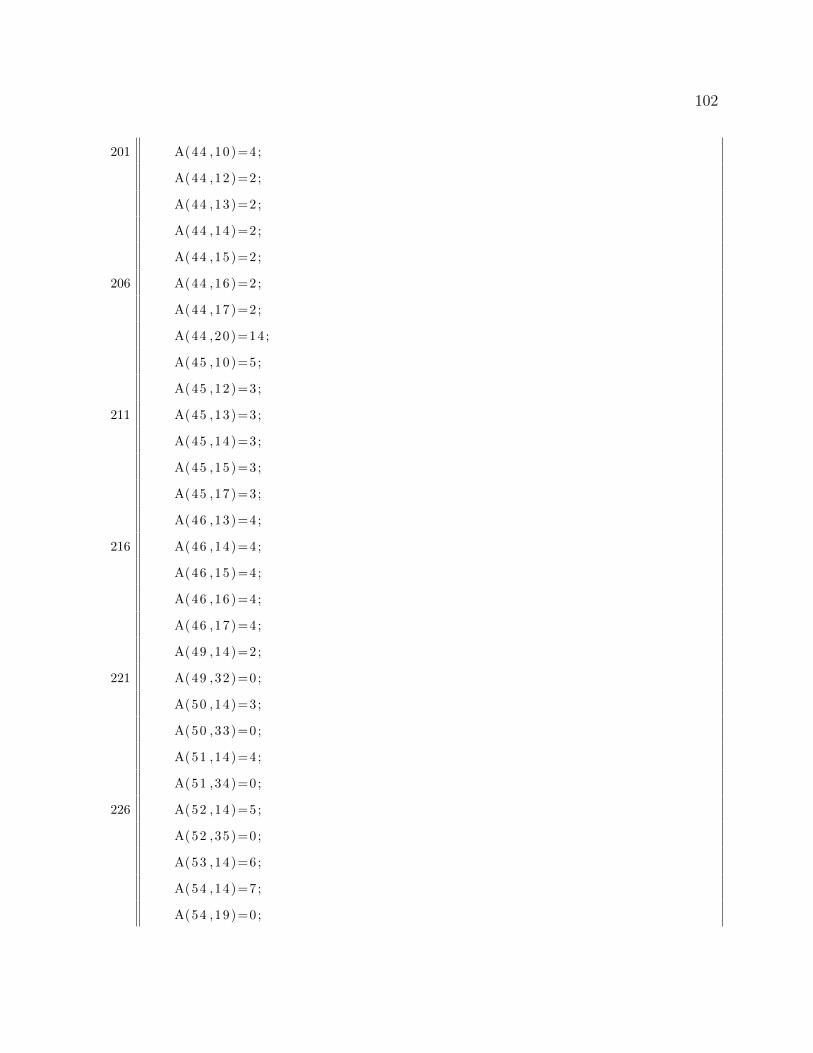
102
201 A(44 ,10)=4;
A(44 ,12)=2;
A(44 ,13)=2;
A(44 ,14)=2;
A(44 ,15)=2;
206 A(44 ,16)=2;
A(44 ,17)=2;
A(44 ,20)=14;
A(45 ,10)=5;
A(45 ,12)=3;
211 A(45 ,13)=3;
A(45 ,14)=3;
A(45 ,15)=3;
A(45 ,17)=3;
A(46 ,13)=4;
216 A(46 ,14)=4;
A(46 ,15)=4;
A(46 ,16)=4;
A(46 ,17)=4;
A(49 ,14)=2;
221 A(49 ,32)=0;
A(50 ,14)=3;
A(50 ,33)=0;
A(51 ,14)=4;
A(51 ,34)=0;
226 A(52 ,14)=5;
A(52 ,35)=0;
A(53 ,14)=6;
A(54 ,14)=7;
A(54 ,19)=0;
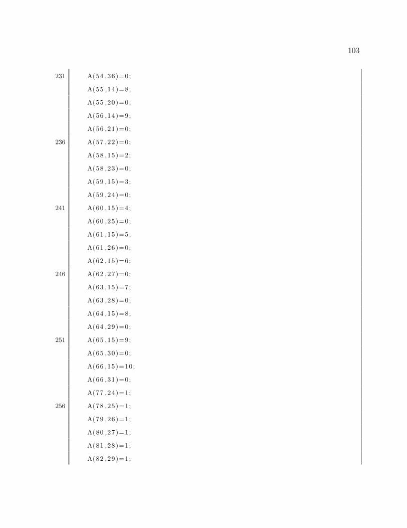
103
231 A(54 ,36)=0;
A(55 ,14)=8;
A(55 ,20)=0;
A(56 ,14)=9;
A(56 ,21)=0;
236 A(57 ,22)=0;
A(58 ,15)=2;
A(58 ,23)=0;
A(59 ,15)=3;
A(59 ,24)=0;
241 A(60 ,15)=4;
A(60 ,25)=0;
A(61 ,15)=5;
A(61 ,26)=0;
A(62 ,15)=6;
246 A(62 ,27)=0;
A(63 ,15)=7;
A(63 ,28)=0;
A(64 ,15)=8;
A(64 ,29)=0;
251 A(65 ,15)=9;
A(65 ,30)=0;
A(66 ,15)=10;
A(66 ,31)=0;
A(77 ,24)=1;
256 A(78 ,25)=1;
A(79 ,26)=1;
A(80 ,27)=1;
A(81 ,28)=1;
A(82 ,29)=1;
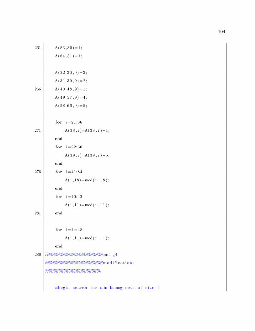
104
261 A(83 ,30)=1;
A(84 ,31)=1;
A(22 :30 ,9 )=3 ;
A(31 :39 ,9 )=2 ;
266 A(40 :48 ,9 )=1 ;
A(49 :57 ,9 )=4 ;
A(58 :66 ,9 )=5 ;
for i =21:36
271 A(38 , i )=A(38 , i ) −1;
end
for i =22:36
A(39 , i )=A(39 , i ) −5;
end
276 for i =41:84
A( i ,18)=mod( i , 1 8 ) ;
end
for i =40:42
A( i ,11)=mod( i , 1 1 ) ;
281 end
for i =44:48
A( i ,11)=mod( i , 1 1 ) ;
end
286 %%%%%%%%%%%%%%%%%%%%%%%end g4
%%%%%%%%%%%%%%%%%%%%%%%m o d i f i c a t i o n s
%%%%%%%%%%%%%%%%%%%%%%
%begin search f o r min homog s e t s o f s i z e 4
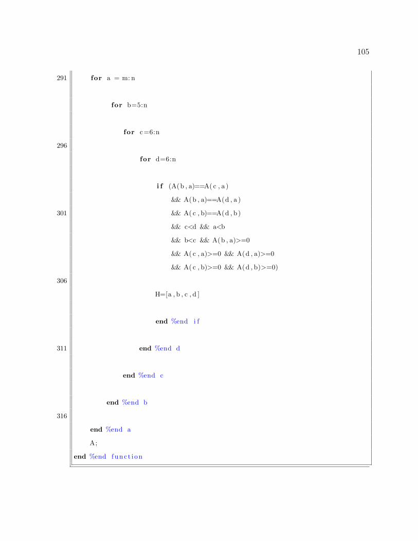
105
291 for a = m: n
for b=5:n
for c =6:n
296
for d=6:n
i f (A(b , a)==A( c , a )
&& A(b , a)==A(d , a )
301 && A( c , b)==A(d , b)
&& c<d && a<b
&& b<c && A(b , a)>=0
&& A( c , a)>=0 && A(d , a)>=0
&& A( c , b)>=0 && A(d , b)>=0)
306
H=[a , b , c , d ]
end %end i f
311 end %end d
end %end c
end %end b
316
end %end a
A;
end %end func t i on
106
Figure A.1: A Matlab function witnessing a regressive function with no min-homogeneous set of size 4
A.2 The Search for Strong Representatives
Recall that a strong representative of order n for a coloring c is a prime
p = nk + 1
such that
ik (mod p)
are pairwise distinct for i ∈ n. Thus to find a strong representative of order n is to
define a satisfactory coloring using n colors.
As discussed in subsection 5.1.1, in two specific cases (when n+1 or 2n+1 is prime),
we are guaranteed the existence of a strong representative of order n. However, outside
these two cases it is an arduous task to find a strong representative of order n. Figure
A.2 gives the Maple code we used to find a strong representatives of order n. Although
the code evolved over time to what is seen below the general search algorithm has
remained unchanged.
A.3 Density Data Collection Code for Strong Representa-
tives of Order 5
Figure A.3 gives the Maple code that was utilized to collect data concerning the
density of primes associated with strong representatives in the case of 5 colors.
Table A.1 represents data collected on the density of satisfactory 5-colorings.
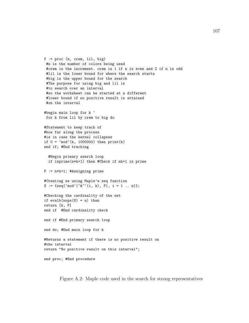
107
f := proc (n, crem, lil, big)
#n is the number of colors being used
#crem is the increment. crem is 1 if n is even and 2 if n is odd
#lil is the lower bound for where the search starts
#big is the upper bound for the search
#The purpose for using big and lil is
#to search over an interval
#so the worksheet can be started at a different
#lower bound if no positive result is attained
#on the interval
#begin main loop for k ‘
for k from lil by crem to big do
#Statement to keep track of
#how far along the process
#is in case the kernel collapses
if 0 = ‘mod‘(k, 1000000) then print(k)
end if; #End tracking
#Begin primary search loop
if isprime(n*k+1) then #Check if nk+1 is prime
P := n*k+1; #Assigning prime
#Creating se using Maple’s seq function
S := {seq(‘mod‘(‘&^‘(i, k), P), i = 1 .. n)};
#Checking the cardinality of the set
if evalb(nops(S) = n) then
return [k, P]
end if #End cardinality check
end if #End primary search loop
end do; #End main loop for k
#Returns a statement if there is no positive result on
#the interval
return "No positive result on this interval";
end proc; #End procedure
Figure A.2: Maple code used in the search for strong representatives
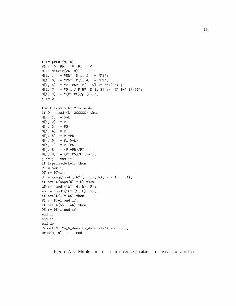
108
f := proc (m, n)
P1 := 0; P5 := 0; PT := 0;
M := Matrix(25, 9);
M[1, 1] := "5k"; M[1, 2] := "P1";
M[1, 3] := "P5"; M[1, 4] := "PT";
M[1, 5] := "P1+P5"; M[1, 6] := "pi(5k)";
M[1, 7] := "P_1 / P_5"; M[1, 8] := "(P_1+P_5)/PT";
M[1, 9] := "(P1+P5)/pi(5k)";
j := 2;
for k from m by 2 to n do
if 0 = ‘mod‘(k, 200000) then
M[j, 1] := 5*k;
M[j, 2] := P1;
M[j, 3] := P5;
M[j, 4] := PT;
M[j, 5] := P1+P5;
M[j, 6] := Pi(5*k);
M[j, 7] := P1/P5;
M[j, 8] := (P1+P5)/PT;
M[j, 9] := (P1+P5)/Pi(5*k);
j := j+1 end if;
if isprime(5*k+1) then
P := 5*k+1;
PT := PT+1;
S := {seq(‘mod‘(‘&^‘(i, k), P), i = 1 .. 5)};
if evalb(nops(S) = 5) then
a6 := ‘mod‘(‘&^‘(6, k), P);
a5 := ‘mod‘(‘&^‘(5, k), P);
if evalb(1 = a6) then
P1 := P1+1 end if;
if evalb(a5 = a6) then
P5 := P5+1 end if
end if
end if
end do;
Export(M, "n_5_density_data.xls") end proc;
proc(m, n) ... end;
Figure A.3: Maple code used for data acquisition in the case of 5 colors
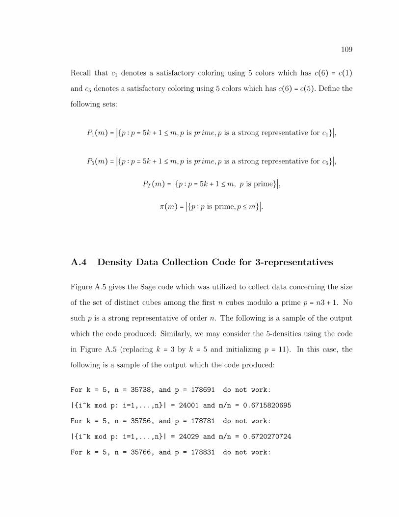
109
Recall that c1 denotes a satisfactory coloring using 5 colors which has c(6) = c(1)
and c5 denotes a satisfactory coloring using 5 colors which has c(6) = c(5). Define the
following sets:
P1(m) = ∣{p ∶ p = 5k + 1 ≤m,p is prime, p is a strong representative for c1}∣,
P5(m) = ∣{p ∶ p = 5k + 1 ≤m,p is prime, p is a strong representative for c5}∣,
PT (m) = ∣{p ∶ p = 5k + 1 ≤m, p is prime}∣,
π(m) = ∣{p ∶ p is prime, p ≤m}∣.
A.4 Density Data Collection Code for 3-representatives
Figure A.5 gives the Sage code which was utilized to collect data concerning the size
of the set of distinct cubes among the first n cubes modulo a prime p = n3 + 1. No
such p is a strong representative of order n. The following is a sample of the output
which the code produced: Similarly, we may consider the 5-densities using the code
in Figure A.5 (replacing k = 3 by k = 5 and initializing p = 11). In this case, the
following is a sample of the output which the code produced:
For k = 5, n = 35738, and p = 178691 do not work:
|{i^k mod p: i=1,...,n}| = 24001 and m/n = 0.6715820695
For k = 5, n = 35756, and p = 178781 do not work:
|{i^k mod p: i=1,...,n}| = 24029 and m/n = 0.6720270724
For k = 5, n = 35766, and p = 178831 do not work:
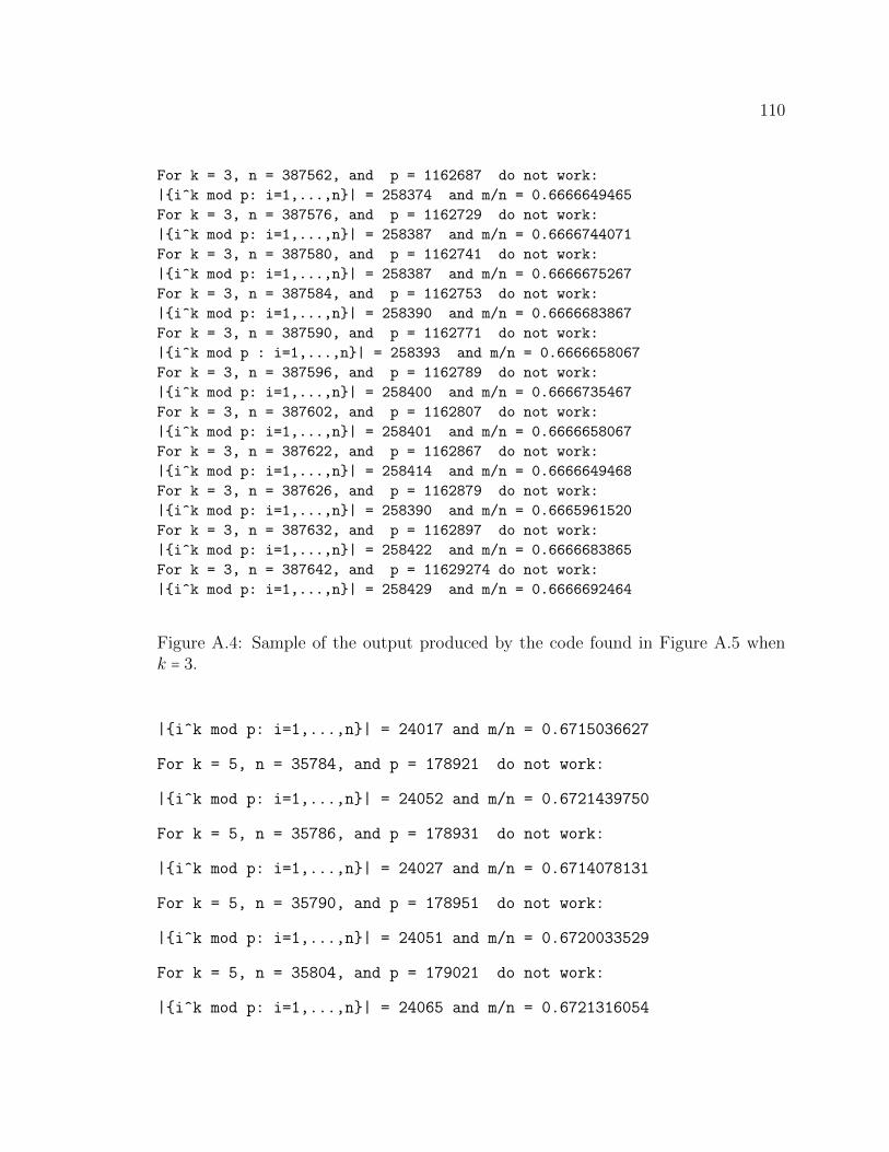
110
For k = 3, n = 387562, and p = 1162687 do not work:
|{i^k mod p: i=1,...,n}| = 258374 and m/n = 0.6666649465
For k = 3, n = 387576, and p = 1162729 do not work:
|{i^k mod p: i=1,...,n}| = 258387 and m/n = 0.6666744071
For k = 3, n = 387580, and p = 1162741 do not work:
|{i^k mod p: i=1,...,n}| = 258387 and m/n = 0.6666675267
For k = 3, n = 387584, and p = 1162753 do not work:
|{i^k mod p: i=1,...,n}| = 258390 and m/n = 0.6666683867
For k = 3, n = 387590, and p = 1162771 do not work:
|{i^k mod p : i=1,...,n}| = 258393 and m/n = 0.6666658067
For k = 3, n = 387596, and p = 1162789 do not work:
|{i^k mod p: i=1,...,n}| = 258400 and m/n = 0.6666735467
For k = 3, n = 387602, and p = 1162807 do not work:
|{i^k mod p: i=1,...,n}| = 258401 and m/n = 0.6666658067
For k = 3, n = 387622, and p = 1162867 do not work:
|{i^k mod p: i=1,...,n}| = 258414 and m/n = 0.6666649468
For k = 3, n = 387626, and p = 1162879 do not work:
|{i^k mod p: i=1,...,n}| = 258390 and m/n = 0.6665961520
For k = 3, n = 387632, and p = 1162897 do not work:
|{i^k mod p: i=1,...,n}| = 258422 and m/n = 0.6666683865
For k = 3, n = 387642, and p = 11629274 do not work:
|{i^k mod p: i=1,...,n}| = 258429 and m/n = 0.6666692464
Figure A.4: Sample of the output produced by the code found in Figure A.5 whenk = 3.
|{i^k mod p: i=1,...,n}| = 24017 and m/n = 0.6715036627
For k = 5, n = 35784, and p = 178921 do not work:
|{i^k mod p: i=1,...,n}| = 24052 and m/n = 0.6721439750
For k = 5, n = 35786, and p = 178931 do not work:
|{i^k mod p: i=1,...,n}| = 24027 and m/n = 0.6714078131
For k = 5, n = 35790, and p = 178951 do not work:
|{i^k mod p: i=1,...,n}| = 24051 and m/n = 0.6720033529
For k = 5, n = 35804, and p = 179021 do not work:
|{i^k mod p: i=1,...,n}| = 24065 and m/n = 0.6721316054
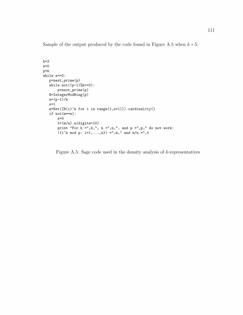
111
Sample of the output produced by the code found in Figure A.5 when k = 5.
k=3
s=0
p=k
while s==0:
p=next_prime(p)
while not((p-1)%k==0):
p=next_prime(p)
R=IntegerModRing(p)
n=(p-1)/k
s=1
m=Set([R(i)^k for i in range(1,n+1)]).cardinality()
if not(m==n):
s=0
t=(m/n).n(digits=10)
print "For k =",k,", n =",n,", and p =",p," do not work:
|{i^k mod p: i=1,...,n}| =",m," and m/n =",t
Figure A.5: Sage code used in the density analysis of k-representatives
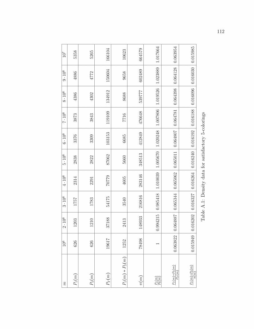
112
m10
62⋅1
063⋅1
064⋅1
065⋅1
066⋅1
067⋅1
068⋅1
069⋅1
0610
7
P1(m
)62
612
0317
5723
1428
3833
7638
7343
8648
8653
58
P5(m
)62
612
1017
8322
9128
2233
0938
4343
0247
7252
65
PT(m
)19
617
3718
854
175
7077
987
062
1031
5311
9109
1349
1215
0604
1661
04
P1(m
)+P5(m
)12
5224
1335
4046
0556
6066
8577
1686
8896
5810
623
π(m
)78
498
1489
3321
6816
2831
4634
8513
4128
4947
6648
5397
7760
2489
6645
79
P1(m)
P5(m)
10.
9942
150.
9854
181.
0100
391.
0056
701.
0202
481.
0078
061.
0195
261.
0238
891.
0176
64
P1(m)+P5(m)
PT(m)
0.06
3822
0.06
4887
0.06
5344
0.06
5062
0.06
5011
0.06
4807
0.06
4781
0.06
4398
0.06
4128
0.06
3954
P1(m)+P5(m)
π(m)
0.01
5949
0.01
6202
0.01
6327
0.01
6264
0.01
6240
0.01
6192
0.01
6188
0.01
6096
0.01
6030
0.01
5985
Tab
leA
.1:
Den
sity
dat
afo
rsa
tisf
acto
ry5-
colo
rings
113
APPENDIX B
PARTIAL HOMOMORPHISM TABLES
The following tables represent explicit constructions of partial homomorphisms for
n ≤ 54. The tables are interpreted as follows. The first column represents the domain
of the partial homomorphisms. The column whose first entry is hn(a) has as its row
entries the image of a partial homomorphism on a set of size n. For example, in Table
B.1, h8(3) = 4. Note that in Tables B.2, B.4, B.3, and B.5 we list only the values for
the primes less than or equal to n2 since having these values allows one to complete
the table.
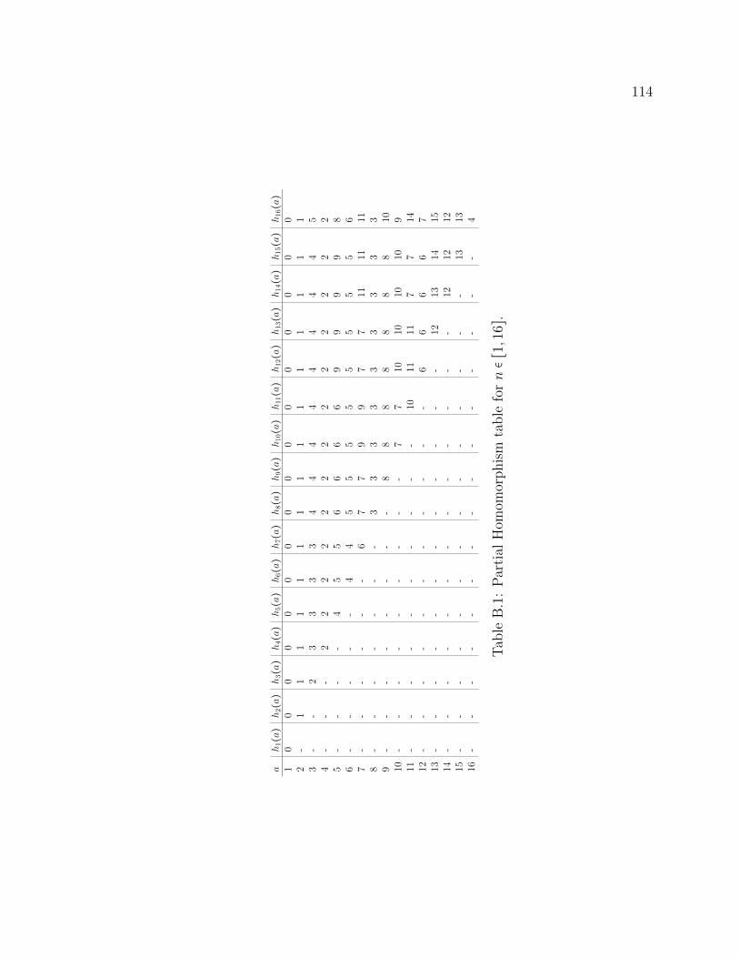
114
ah1(a
)h2(a
)h3(a
)h4(a
)h5(a
)h6(a
)h7(a
)h8(a
)h9(a
)h10(a
)h11(a
)h12(a
)h13(a
)h14(a
)h15(a
)h16(a
)1
00
00
00
00
00
00
00
00
2-
11
11
11
11
11
11
11
13
--
23
33
34
44
44
44
45
4-
--
22
22
22
22
22
22
25
--
--
45
56
66
69
99
98
6-
--
--
44
55
55
55
55
67
--
--
--
67
79
97
711
1111
8-
--
--
--
33
33
33
33
39
--
--
--
--
88
88
88
810
10-
--
--
--
--
77
1010
1010
911
--
--
--
--
--
1011
117
714
12-
--
--
--
--
--
66
66
713
--
--
--
--
--
--
1213
1415
14-
--
--
--
--
--
--
1212
1215
--
--
--
--
--
--
--
1313
16-
--
--
--
--
--
--
--
4
Tab
leB
.1:
Par
tial
Hom
omor
phis
mta
ble
forn∈[
1,16
].
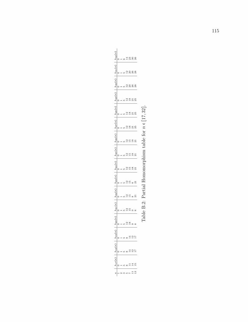
115
ah17(a)
h18(a)
h19(a)
h20(a)
h21(a)
h22(a)
h23(a)
h24(a)
h25(a)
h26(a)
h27(a)
h28(a)
h29(a)
h30(a)
h31(a)
h32(a)
10
00
00
00
00
00
00
00
02
11
11
11
11
11
11
11
11
35
55
55
55
55
55
55
55
65
88
812
12
12
12
12
12
12
12
12
12
12
12
14
711
14
14
18
15
15
15
15
15
15
18
18
18
20
20
23
11
14
12
12
99
88
18
18
18
21
21
21
26
26
30
13
15
17
17
88
21
21
21
21
21
25
25
25
28
28
26
Tab
leB
.2:
Par
tial
Hom
omor
phis
mta
ble
forn∈[
17,3
2].
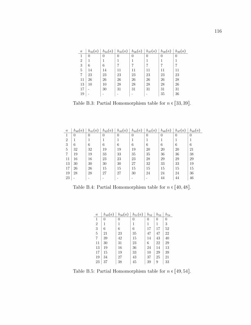
116
a h33(a) h34(a) h35(a) h36(a) h37(a) h38(a) h39(a)1 0 0 0 0 0 0 02 1 1 1 1 1 1 13 6 6 7 7 7 7 75 14 14 11 11 11 11 117 23 23 23 23 23 23 2311 26 26 26 26 26 26 2813 10 10 28 28 28 28 2617 - 30 31 31 31 31 3119 - - - - - 35 36
Table B.3: Partial Homomorphism table for n ∈ [33,39].
a h40(a) h41(a) h42(a) h43(a) h44(a) h45(a) h46(a) h47(a) h48(a)1 0 0 0 0 0 0 0 0 02 1 1 1 1 1 1 1 1 13 6 6 6 6 6 6 6 6 65 32 32 19 19 19 20 20 20 217 19 19 33 33 35 35 36 36 3811 16 16 23 23 23 28 29 29 2913 30 30 30 30 27 32 33 33 1917 26 26 15 15 15 15 15 15 1519 28 28 27 27 30 24 24 24 3623 - - - - - - 44 44 46
Table B.4: Partial Homomorphism table for n ∈ [40,48].
a h49(a) h50(a) h51(a) h52 h53 h541 0 0 0 0 0 02 1 1 1 1 1 33 6 6 6 17 17 525 21 23 35 47 47 227 39 42 15 14 43 4011 30 31 23 6 22 2913 19 16 36 24 14 1317 15 19 33 10 29 3919 34 27 43 37 25 2123 37 38 45 39 9 33
Table B.5: Partial Homomorphism table for n ∈ [49,54].
117
APPENDIX C
GROUPLESS n
The data found in Table C.1 was supplied by Rodney Forcade. The table lists all
groupless values of n ≤ 500. The data was obtained via an exhaustive search algorithm
implemented by a computer. Note that for all values of n ≤ 500 not listed in the table,
at least one of the following is true:
1. n + 1 is prime,
2. 2n + 1 is prime,
3. The existence of a G-satisfactory group has been verified.
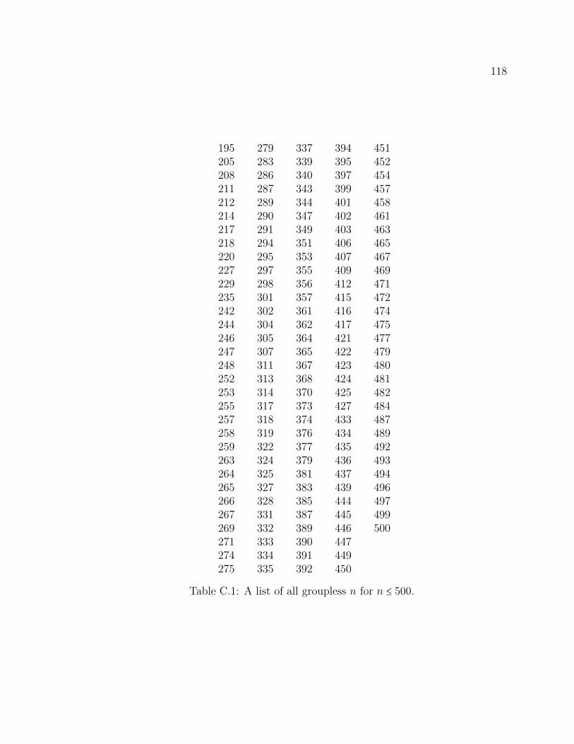
118
195 279 337 394 451205 283 339 395 452208 286 340 397 454211 287 343 399 457212 289 344 401 458214 290 347 402 461217 291 349 403 463218 294 351 406 465220 295 353 407 467227 297 355 409 469229 298 356 412 471235 301 357 415 472242 302 361 416 474244 304 362 417 475246 305 364 421 477247 307 365 422 479248 311 367 423 480252 313 368 424 481253 314 370 425 482255 317 373 427 484257 318 374 433 487258 319 376 434 489259 322 377 435 492263 324 379 436 493264 325 381 437 494265 327 383 439 496266 328 385 444 497267 331 387 445 499269 332 389 446 500271 333 390 447274 334 391 449275 335 392 450
Table C.1: A list of all groupless n for n ≤ 500.


![Juan Caicedo - Amazon S3s3.amazonaws.com/zanran_storage/€¦ · Juan Caicedo From: Pronczuk, Jenny [pronczukj@who.int] Sent: 30 June 2006 18:29 To: Juan Caicedo Cc: Meredith, Tim;](https://static.documents.pub/doc/80x56/5ba3b6cf09d3f2205e8bdeea/juan-caicedo-amazon-s3s3-juan-caicedo-from-pronczuk-jenny-pronczukjwhoint.jpg)
