
© Fluent Inc. 04/22/231
Fluent Software TrainingMTG-97-183
Combustion Modelingin FLUENT
© Fluent Inc. 04/22/232
Fluent Software TrainingMTG-97-183
Outline
Applications Overview of Combustion Modeling Capabilities Chemical Kinetics Gas Phase Combustion Models Discrete Phase Models Pollutant Models Combustion Simulation Guidelines
© Fluent Inc. 04/22/233
Fluent Software TrainingMTG-97-183
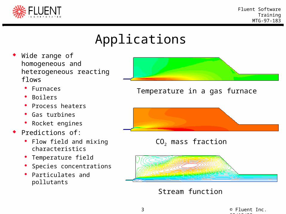
Applications Wide range of homogeneous
and heterogeneous reacting flows
Furnaces Boilers Process heaters Gas turbines Rocket engines
Predictions of: Flow field and mixing
characteristics Temperature field Species concentrations Particulates and pollutants
Temperature in a gas furnace
CO2 mass fraction
Stream function

© Fluent Inc. 04/22/234
Fluent Software TrainingMTG-97-183
Aspects of Combustion Modeling
Dispersed Phase Models
Droplet/particle dynamicsHeterogeneous reactionDevolatilizationEvaporation
Governing Transport EquationsMassMomentum (turbulence)EnergyChemical Species
Combustion ModelsPremixedPartially premixedNonpremixed
Pollutant Models Radiative Heat Transfer Models
© Fluent Inc. 04/22/235
Fluent Software TrainingMTG-97-183
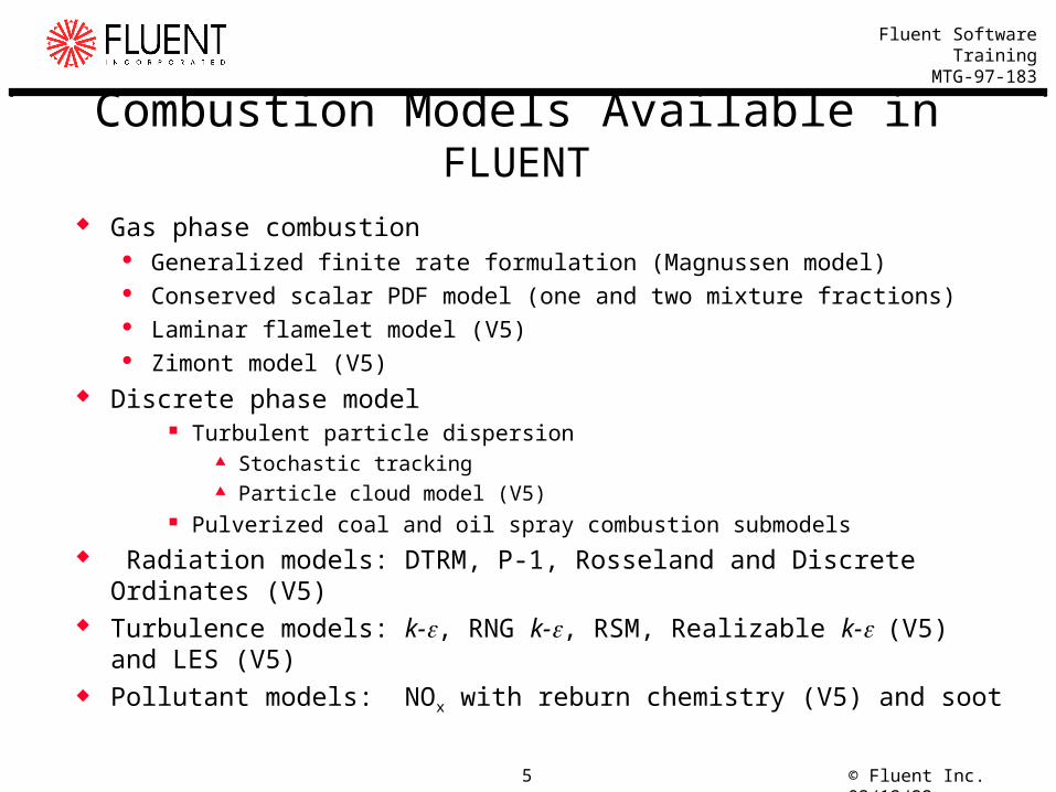
Gas phase combustion Generalized finite rate formulation (Magnussen model) Conserved scalar PDF model (one and two mixture fractions) Laminar flamelet model (V5) Zimont model (V5)
Discrete phase model Turbulent particle dispersion
Stochastic tracking Particle cloud model (V5)
Pulverized coal and oil spray combustion submodels Radiation models: DTRM, P-1, Rosseland and Discrete Ordinates (V5) Turbulence models: k-, RNG k-, RSM, Realizable k-(V5) and LES (V5) Pollutant models: NOx with reburn chemistry (V5) and soot
Combustion Models Available in FLUENT
© Fluent Inc. 04/22/236
Fluent Software TrainingMTG-97-183
Modeling Chemical Kinetics in Combustion Challenging
Most practical combustion processes are turbulent Rate expressions are highly nonlinear; turbulence-chemistry interactions
are important Realistic chemical mechanisms have tens of species, hundreds of
reactions and stiff kinetics (widely disparate time scales) Practical approaches
Reduced chemical mechanisms Finite rate combustion model
Decouple reaction chemistry from turbulent flow and mixing Mixture fraction approaches
Equilibrium chemistry PDF model Laminar flamelet
Progress variable Zimont model
© Fluent Inc. 04/22/237
Fluent Software TrainingMTG-97-183
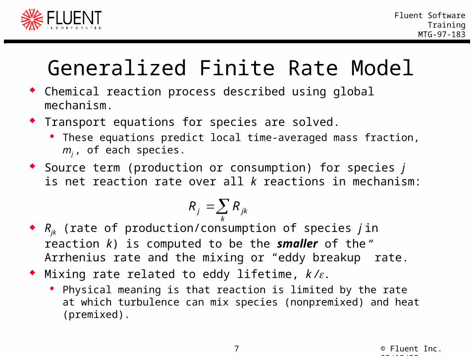
Generalized Finite Rate Model Chemical reaction process described using global mechanism. Transport equations for species are solved.
These equations predict local time-averaged mass fraction, mj , of each species.
Source term (production or consumption) for species j is net reaction rate over all k reactions in mechanism:
Rjk (rate of production/consumption of species j in reaction k) is computed to be the smaller of the Arrhenius rate and the mixing or “eddy breakup” rate.
Mixing rate related to eddy lifetime, k /. Physical meaning is that reaction is limited by the rate at which turbulence
can mix species (nonpremixed) and heat (premixed).
R Rj jkk
© Fluent Inc. 04/22/238
Fluent Software TrainingMTG-97-183
Setup of Finite Rate Chemistry Models
Requires: List of species and their properties List of reactions and reaction rates
FLUENT V5 provides this info in a mixture material database. Chemical mechanisms and physical properties for the most common
fuels are provided in database. If you have different chemistry, you can:
Create new mixtures. Modify properties/reactions of existing mixtures.
© Fluent Inc. 04/22/239
Fluent Software TrainingMTG-97-183
Generalized Finite Rate Model: Summary
Advantages: Applicable to nonpremixed, partially premixed, and premixed combustion Simple and intuitive Widely used
Disadvantages: Unreliable when mixing and kinetic time scales are comparable (requires
Da >>1). No rigorous accounting for turbulence-chemistry interactions Difficulty in predicting intermediate species and accounting for
dissociation effects. Uncertainty in model constants, especially when applied to multiple
reactions.

© Fluent Inc. 04/22/2310
Fluent Software TrainingMTG-97-183
Conserved Scalar (Mixture Fraction) Approach: The PDF Model
Applies to nonpremixed (diffusion) flames only Assumes that reaction is mixing-limited
Local chemical equilibrium conditions prevail. Composition and properties in each cell defined by extent of turbulent
mixing of fuel and oxidizer streams. Reaction mechanism is not explicitly defined by you.
Reacting system treated using chemical equilibrium calculations (prePDF). Solves transport equations for mixture fraction and its variance, rather
than species transport equations. Rigorous accounting of turbulence-chemistry interactions.
© Fluent Inc. 04/22/2311
Fluent Software TrainingMTG-97-183
Mixture Fraction Definition
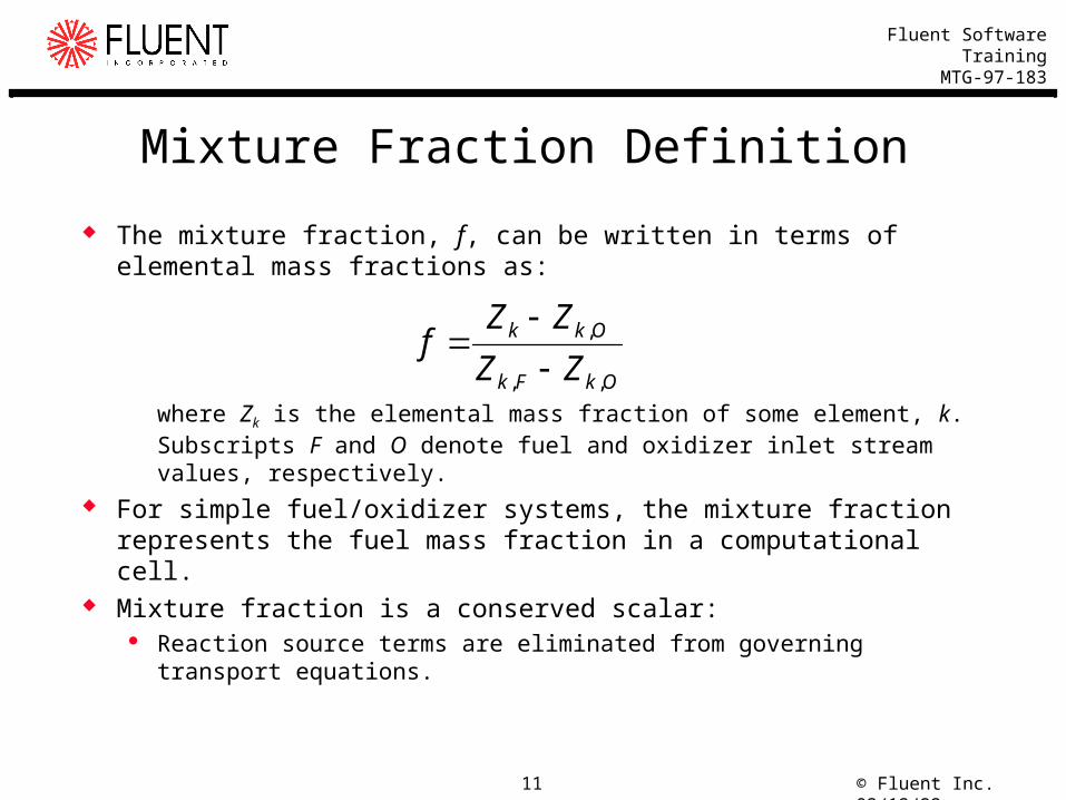
The mixture fraction, f, can be written in terms of elemental mass fractions as:
where Zk is the elemental mass fraction of some element, k. Subscripts F and O denote fuel and oxidizer inlet stream values, respectively.
For simple fuel/oxidizer systems, the mixture fraction represents the fuel mass fraction in a computational cell.
Mixture fraction is a conserved scalar: Reaction source terms are eliminated from governing transport equations.
OkFk
Okk
ZZZZ
f,,
,

© Fluent Inc. 04/22/2312
Fluent Software TrainingMTG-97-183
Systems That Can be Modeled Using a Single Mixture Fraction
Fuel/air diffusion flame:
Diffusion flame with oxygen-enriched inlets:
System using multiple fuel inlets:
60% CH4 40% CO21% O2 79% N2
f = 1
f = 035% O2 65% N2
60% CH4 40% CO35% O2 65% N2
f = 1
f = 0
f = 0
60% CH4 20% CO 10% C3H8 10% CO2
21% O2 79% N2
f = 1
f = 0
f = 1
60% CH4 20% CO 10% C3H8 10% CO2

© Fluent Inc. 04/22/2313
Fluent Software TrainingMTG-97-183
Equilibrium Approximation of System Chemistry
Chemistry is assumed to be fast enough to achieve equilibrium. Intermediate species are included.

© Fluent Inc. 04/22/2314
Fluent Software TrainingMTG-97-183
PDF Modeling of Turbulence-Chemistry Interaction Fluctuating mixture fraction is completely defined by its probability density
function (PDF).
p(V), the PDF, represents fraction of sampling time when variable, V, takes a value between V and V + V.
p(f) can be used to compute time-averaged values of variables that depend on the mixture fraction, f:
Species mole fractions Temperature, density
p V VTT i
i( ) lim
1
© Fluent Inc. 04/22/2315
Fluent Software TrainingMTG-97-183
PDF Model Flexibility Nonadiabatic systems:
In real problems, with heat loss or gain, local thermo-chemical state must be related to mixture fraction, f, and enthalpy, h.
Average quantities now evaluated as a function of mixture fraction, enthalpy (normalized heat loss/gain), and the PDF, p(f).
Second conserved scalar: With second scalar in FLUENT, you can model:
Two fuel streams with different compositions and single oxidizer stream (visa versa)
Nonreacting stream in addition to a fuel and an oxidizer Co-firing a gaseous fuel with another gaseous, liquid, or coal fuel Firing single coal with two off-gases (volatiles and char burnout products)
tracked separately
© Fluent Inc. 04/22/2316
Fluent Software TrainingMTG-97-183
Mixture Fraction/PDF Model: Summary
Advantages: Predicts formation of intermediate species. Accounts for dissociation effects. Accounts for coupling between turbulence and chemistry. Does not require the solution of a large number of species transport
equations Robust and economical
Disadvantages: System must be near chemical equilibrium locally. Cannot be used for compressible or non-turbulent flows. Not applicable to premixed systems.
© Fluent Inc. 04/22/2317
Fluent Software TrainingMTG-97-183
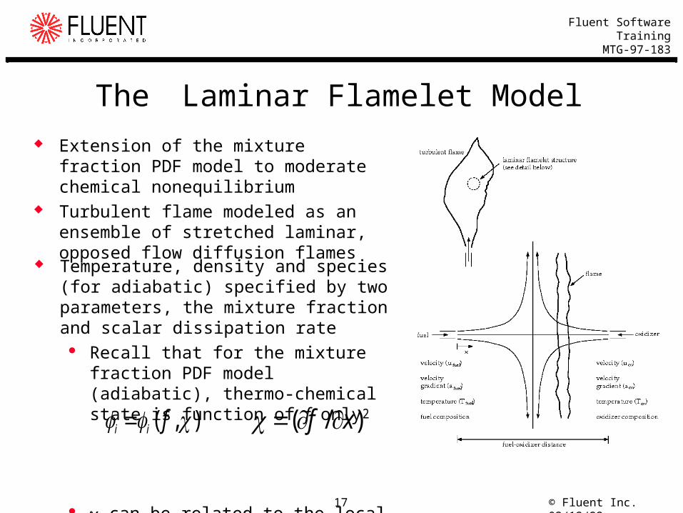
The Laminar Flamelet Model
Temperature, density and species (for adiabatic) specified by two parameters, the mixture fraction and scalar dissipation rate
Recall that for the mixture fraction PDF model (adiabatic), thermo-chemical state is function of f only
can be related to the local rate of strain
Extension of the mixture fraction PDF model to moderate chemical nonequilibrium
Turbulent flame modeled as an ensemble of stretched laminar, opposed flow diffusion flames
2)/( xf ),( fii
© Fluent Inc. 04/22/2318
Fluent Software TrainingMTG-97-183
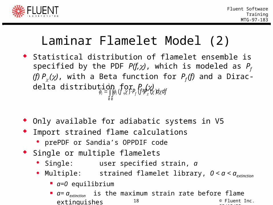
Laminar Flamelet Model (2) Statistical distribution of flamelet ensemble is specified by the PDF
P(f,), which is modeled as Pf (f) P (), with a Beta function for Pf (f) and a Dirac-delta distribution for P ()
Only available for adiabatic systems in V5 Import strained flame calculations
prePDF or Sandia’s OPPDIF code Single or multiple flamelets
Single: user specified strain, a Multiple: strained flamelet library, 0 < a < aextinction
a=0 equilibrium a= aextinction is the maximum strain rate before flame extinguishes
Possible to model local extinction pockets (e.g. lifted flames)
1
0 0
)()(),( dfdPfPf fii

© Fluent Inc. 04/22/2319
Fluent Software TrainingMTG-97-183
The Zimont Model for Premixed Combustion Thermo-chemistry described by a single progress variable,
Mean reaction rate, Turbulent flame speed, Ut, derived for lean premixed combustion and
accounts for Equivalence ratio of the premixed fuel Flame front wrinkling and thickening by turbulence Flame front quenching by turbulent stretching Differential molecular diffusion
For adiabatic combustion,
The enthalpy equation must be solved for nonadiabatic combustion
tc
xu c
x Sccx
R ci
ii
t
t ic
0 1
R U cc unburnt t
p
adp
pp YYc /
adunburnt TcTcT )1(
© Fluent Inc. 04/22/2320
Fluent Software TrainingMTG-97-183
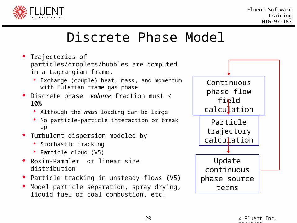
Discrete Phase Model Trajectories of particles/droplets/bubbles are
computed in a Lagrangian frame. Exchange (couple) heat, mass, and momentum
with Eulerian frame gas phase Discrete phase volume fraction must < 10%
Although the mass loading can be large No particle-particle interaction or break up
Turbulent dispersion modeled by Stochastic tracking Particle cloud (V5)
Rosin-Rammler or linear size distribution Particle tracking in unsteady flows (V5) Model particle separation, spray drying, liquid
fuel or coal combustion, etc.
Continuous phase flow field calculation
Particle trajectory calculation
Update continuous phase source terms
© Fluent Inc. 04/22/2321
Fluent Software TrainingMTG-97-183
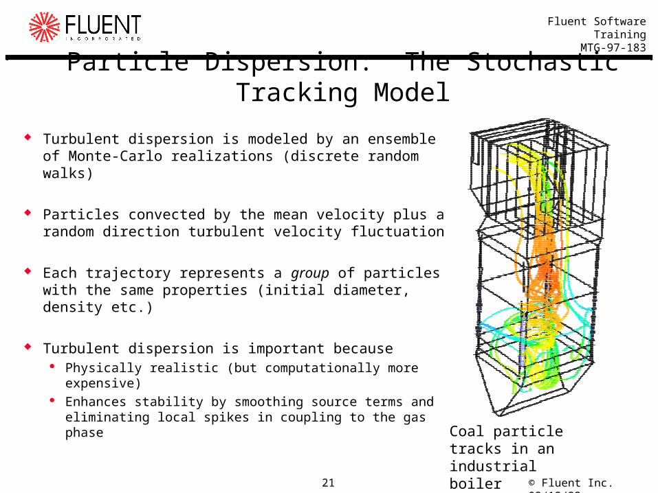
Turbulent dispersion is modeled by an ensemble of Monte-Carlo realizations (discrete random walks)
Particles convected by the mean velocity plus a random direction turbulent velocity fluctuation
Each trajectory represents a group of particles with the same properties (initial diameter, density etc.)
Turbulent dispersion is important because Physically realistic (but computationally more expensive) Enhances stability by smoothing source terms and
eliminating local spikes in coupling to the gas phase
Particle Dispersion: The Stochastic Tracking Model
Coal particle tracks in an industrial boiler

© Fluent Inc. 04/22/2322
Fluent Software TrainingMTG-97-183
Particle Dispersion: The Particle Cloud Model
Track mean particle trajectory along mean velocity Assuming a 3D multi-variate Gaussian distribution about this mean
track, calculate particle loading within three standard deviations Rigorously accounts for inertial and drift velocities A particle cloud is required for each particle type (e.g. initial d, etc.) Particles can escape, reflect or trap (release volatiles) at walls Eliminates (single cloud) or reduces (few clouds) stochastic tracking
Decreased computational expense Increased stability since distributed source terms in gas phase
BUT decreased accuracy since Gas phase properties (e.g. temperature) are averaged within cloud Poor prediction of large recirculation zones

© Fluent Inc. 04/22/2323
Fluent Software TrainingMTG-97-183
Particle Tracking in Unsteady Flows Each particle advanced in time along with the flow For coupled flows using implicit time stepping, sub-iterations for the particle
tracking are performed within each time step For non-coupled flows or coupled flows with explicit time stepping, particles
are advanced at the end of each time step

© Fluent Inc. 04/22/2324
Fluent Software TrainingMTG-97-183
Coal/Oil Combustion Models
Coal or oil combustion modeled by changing the modeled particle to Droplet - for oil combustion Combusting particle - for coal combustion
Several devolatilization and char burnout models provided. Note: These models control the rate of evolution of the fuel off-gas from
coal/oil particles. Reactions in the gas (continuous) phase are modeled with the PDF or finite rate combustion model.

© Fluent Inc. 04/22/2325
Fluent Software TrainingMTG-97-183
NOx Models NOx consists of mostly nitric oxide (NO).
Precursor for smog Contributes to acid rain Causes ozone depletion
Three mechanisms included in FLUENT for NOx production: Thermal NOx - Zeldovich mechanism (oxidation of atmospheric N)
Most significant at high temperatures Prompt NOx - empirical mechanisms by De Soete, Williams, etc.
Contribution is in general small Significant at fuel rich zones
Fuel NOx - Empirical mechanisms by De Soete, Williams, etc. Predominant in coal flames where fuel-bound nitrogen is high and
temperature is generally low. NOx reburn chemistry (V5)
NO can be reduced in fuel rich zones by reaction with hydrocarbons
© Fluent Inc. 04/22/2326
Fluent Software TrainingMTG-97-183
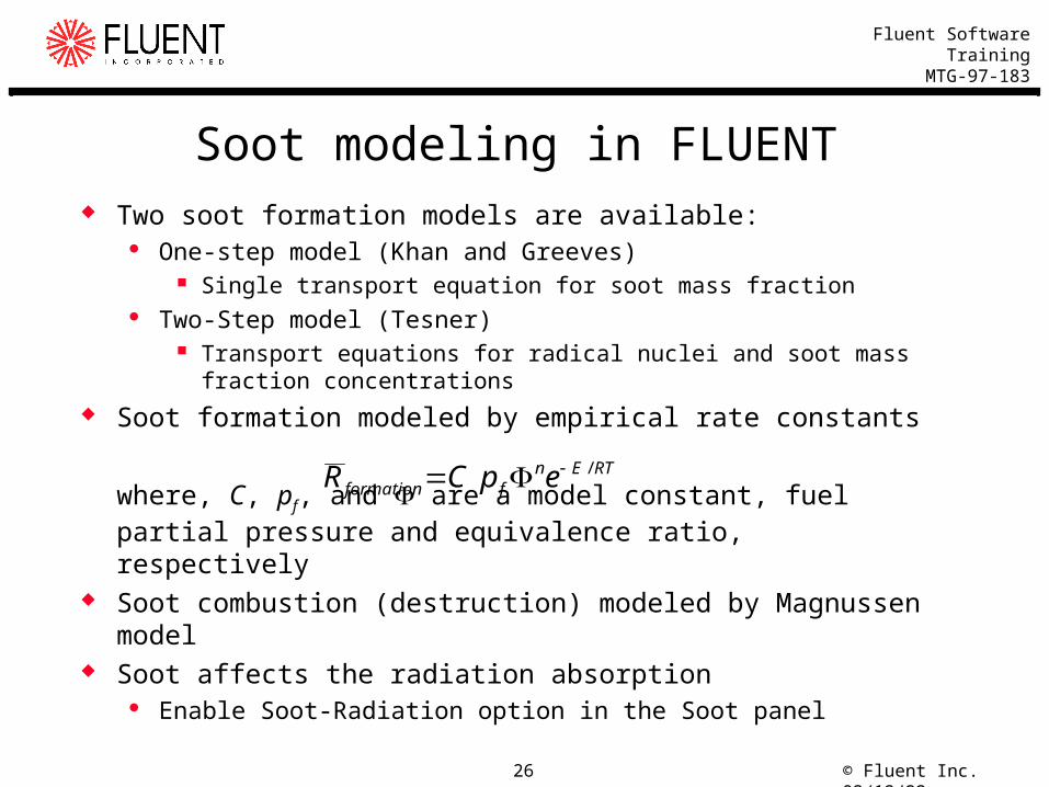
Soot modeling in FLUENT Two soot formation models are available:
One-step model (Khan and Greeves) Single transport equation for soot mass fraction
Two-Step model (Tesner) Transport equations for radical nuclei and soot mass fraction
concentrations Soot formation modeled by empirical rate constants
where, C, pf, and are a model constant, fuel partial pressure and equivalence ratio, respectively
Soot combustion (destruction) modeled by Magnussen model Soot affects the radiation absorption
Enable Soot-Radiation option in the Soot panel
RTEnfformation epCR /

© Fluent Inc. 04/22/2327
Fluent Software TrainingMTG-97-183
Combustion Guidelines and Solution Strategies Start in 2D
Determine applicability of model physics Mesh resolution requirements (resolve shear layers) Solution parameters and convergence settings
Boundary conditions Combustion is often very sensitive to inlet boundary conditions
Correct velocity and scalar profiles can be critical Wall heat transfer is challenging to predict; if known, specify wall
temperature instead of external convection/radiation BC Initial conditions
While steady-state solution is independent of the IC, poor IC may cause divergence due to the number and nonlinearity of the transport equations
Cold flow solution, then gas combustion, then particles, then radiation For strongly swirling flows, increase the swirl gradually

© Fluent Inc. 04/22/2328
Fluent Software TrainingMTG-97-183
Combustion Guidelines and Solution Strategies (2) Underrelaxation Factors
The effect of under-relaxation is highly nonlinear Decrease the diverging residual URF in increments of 0.1 Underrelax density when using the mixture fraction PDF model (0.5) Underrelax velocity for high bouyancy flows Underrelax pressure for high speed flows
Once solution is stable, attempt to increase all URFs to as close to defaults as possible (and at least 0.9 for T, P-1, swirl and species (or mixture fraction statistics))
Discretization Start with first order accuracy, then converge with second order to improve accuracy Second order discretization especially important for tri/tet meshes
Discrete Phase Model - to increase stability, Increase number of stochastic tracks (or use particle cloud model) Decrease DPM URF and increase number of gas phase iterations per DPM
© Fluent Inc. 04/22/2329
Fluent Software TrainingMTG-97-183
Combustion Guidelines and Solution Strategies (3)
Magnussen model Defaults to finite rate/eddy-dissipation (Arrhenius/Magnussen)
For nonpremixed (diffusion) flames turn off finite rate Premixed flames require Arrhenius term so that reactants don’t burn
prematurely May require a high temperature initialization/patch Use temperature dependent Cp’s to reduce unrealistically high temperatures
Mixture fraction PDF model Model of choice if underlying assumptions are valid Use adequate numbers of discrete points in look up tables to ensure accurate
interpolation (no affect on run-time expense) Use beta PDF shape
© Fluent Inc. 04/22/2330
Fluent Software TrainingMTG-97-183
Combustion Guidelines and Solution Strategies (4)
Turbulence Start with standard k- model Switch to RNG k- , Realizable k- or RSM to obtain better agreement
with data and/or to analyze sensitivity to the turbulence model Judging Convergence
Residuals should be less than 10-3 except for T, P-1 and species, which should be less than 10-6
The mass and energy flux reports must balance Monitor variables of interest (e.g. mean temperature at the outlet) Ensure contour plots of field variables are smooth, realistic and steady

© Fluent Inc. 04/22/2331
Fluent Software TrainingMTG-97-183
Concluding Remarks
FLUENT V5 is the code of choice for combustion modeling. Outstanding set of physical models Maximum convenience and ease of use
Built-in database of mechanisms and physical properties Grid flexibility and solution adaption
A wide range of reacting flow applications can be addressed by the combustion models in FLUENT.
Make sure the physical models you are using are appropriate for your application.


