
Comparing Mean Vectors for SeveralPopulations
• Compare mean vectors for g treatments (or populations).
• Randomly assign n` units to the `-th treatment (or takeindependent random samples from g populations)
• Measure p characteristics of each unit. Observation vectorsfor the `-th population
Pop ` : x`1, x`2, ..., x`n`, ` = 1, ..., g.
are p× 1 vectors of measurements. We use x̄` to denote thesample mean vector for the `th treatment, and S` to denotethe estimated covariance matrix in the `th group.
• Each unit responds independently of any other unit.
• We will use n to denote the total sample size: n =∑` n`.
364
Comparing Several Mean Vectors
• If all n`−p are large, the following assumptions are all we needto make inferences about the difference between treatments:
1. X`1, X`2, ..., X`n` ∼ p-variate distribution(µ`,Σ`).
2. Each unit responds independently of any other unit (unitsare randomly allocated to the g treatment groups).
3. Covariance matrices are homogeneous: Σ` = Σ for allgroups.
4. Each unit responds independently of any other unit.
• When samples sizes are small, we use more assumptions:
1. Distributions are multivariate normal.
365
Pooled estimate of the covariance matrix
• If all population covariance matrices are the same, then allgroup-level matrices of sums of squares and cross-productsestimate the same quantity.
• Then, it is reasonable to combine all the group-levelcovariance matrices into a single estimate by computingthe weighted average of the covariance matrices. Weightsare proportional to the number of units in each treatmentgroup.
• The pooled estimate of the common covariance matrix is
Spool =g∑
`=1
(n` − 1)∑gj=1(nj − 1)
S`.366
Analysis of Variance (ANOVA)
• To develop approaches to compare g multivariate means, it
will be convenient to make use of the usual decomposition
of the variability in the sample response vectors into two
sources:
1. Variability due to differences in treatment mean vectors
(between-group variation)
2. Variability due to measurement error or differences among
units within treatment groups( within-group variation)
• We review some of these concepts in the univariate setting,
when p = 1.
367
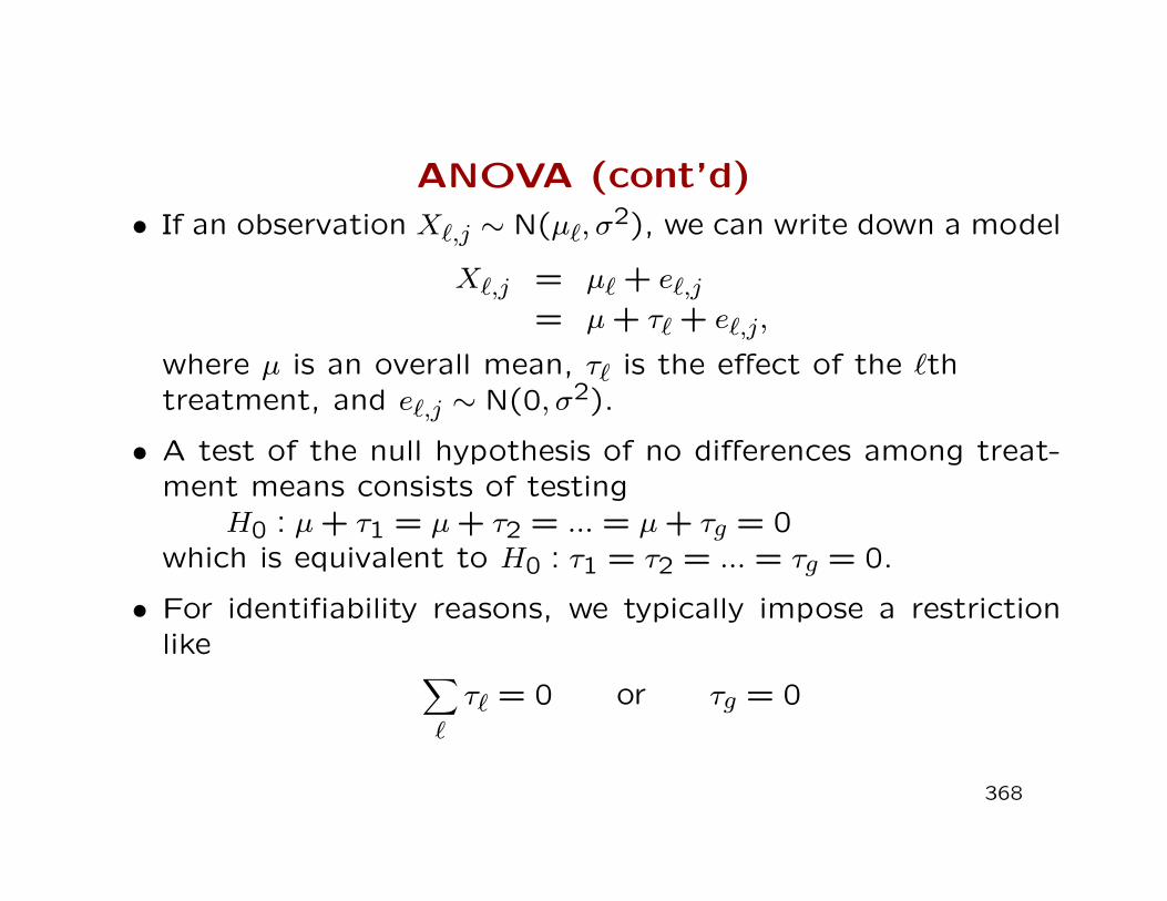
ANOVA (cont’d)
• If an observation X`,j ∼ N(µ`, σ2), we can write down a model
X`,j = µ` + e`,j= µ+ τ` + e`,j,
where µ is an overall mean, τ` is the effect of the `thtreatment, and e`,j ∼ N(0, σ2).
• A test of the null hypothesis of no differences among treat-ment means consists of testing
H0 : µ+ τ1 = µ+ τ2 = ... = µ+ τg = 0which is equivalent to H0 : τ1 = τ2 = ... = τg = 0.
• For identifiability reasons, we typically impose a restrictionlike ∑
`
τ` = 0 or τg = 0
368
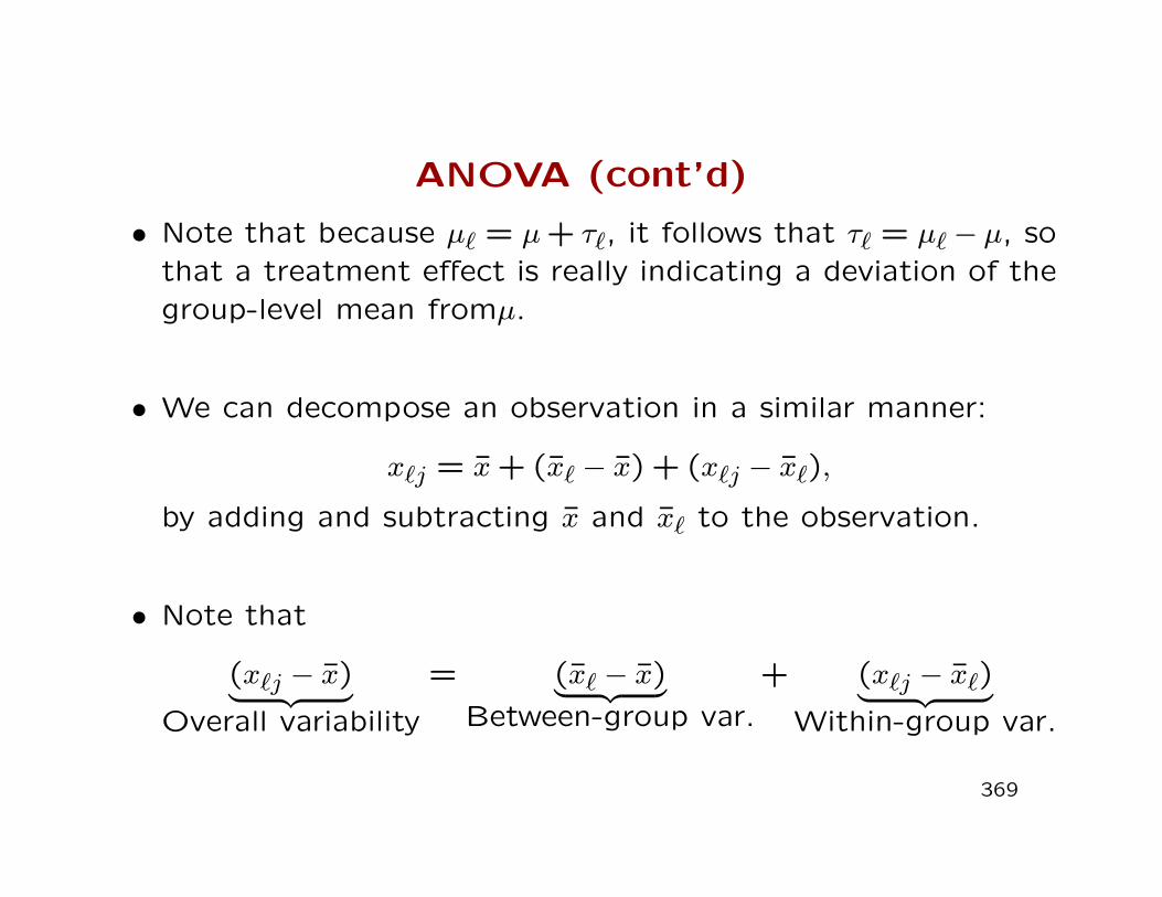
ANOVA (cont’d)
• Note that because µ` = µ+ τ`, it follows that τ` = µ`− µ, sothat a treatment effect is really indicating a deviation of thegroup-level mean fromµ.
• We can decompose an observation in a similar manner:
x`j = x̄+ (x̄` − x̄) + (x`j − x̄`),
by adding and subtracting x̄ and x̄` to the observation.
• Note that
(x`j − x̄)︸ ︷︷ ︸Overall variability
= (x̄` − x̄)︸ ︷︷ ︸Between-group var.
+ (x`j − x̄`)︸ ︷︷ ︸Within-group var.
369

ANOVA (cont’d)
• If we first square both sides of the above expression and sum
over all n` observations in the group and over all groups we
have
(x`j − x̄)2 = (x̄` − x̄)2 + (x`j − x̄`)2 + 2(x̄` − x̄)(x`j − x̄`)
andg∑
`=1
n∑̀j=1
(x`j − x̄)2 =g∑
`=1
n∑̀j=1
(x̄` − x̄)2 +g∑
`=1
n∑̀j=1
(x`j − x̄`)2
=g∑
`=1
n`(x̄` − x̄)2 +g∑
`=1
n∑̀j=1
(x`j − x̄`)2
= SSTreatments + SSError.
370

ANOVA (cont’d)
• The null hypothesis of equal treatment means is rejected at
level α if
F =SSTreatments/(g − 1)
SSError/(n− g)> F(g−1,n−g),α
371
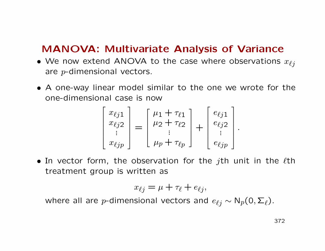
MANOVA: Multivariate Analysis of Variance• We now extend ANOVA to the case where observations x`j
are p-dimensional vectors.
• A one-way linear model similar to the one we wrote for theone-dimensional case is now
x`j1x`j2
...x`jp
=
µ1 + τ`1µ2 + τ`2
...µp + τ`p
+
e`j1e`j2
...e`jp
.
• In vector form, the observation for the jth unit in the `thtreatment group is written as
x`j = µ+ τ` + e`j,
where all are p-dimensional vectors and e`j ∼ Np(0,Σ`).
372
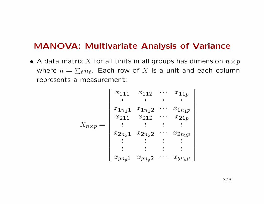
MANOVA: Multivariate Analysis of Variance
• A data matrix X for all units in all groups has dimension n×pwhere n =
∑` n`. Each row of X is a unit and each column
represents a measurement:
Xn×p =
x111 x112 · · · x11p... ... ... ...
x1n11 x1n12 · · · x1n1px211 x212 · · · x21p
... ... ... ...x2n21 x2n22 · · · x2n2p... ... ... ...
... ... ... ...xgng1 xgng2 · · · xgngp
373
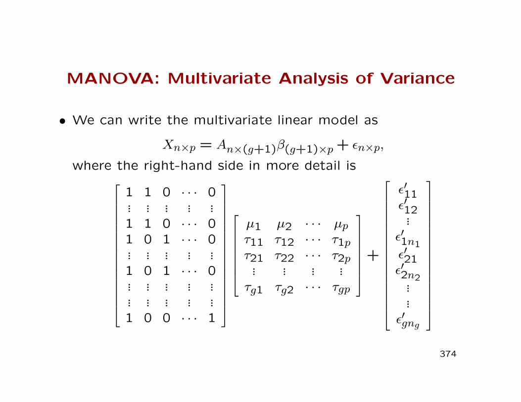
MANOVA: Multivariate Analysis of Variance
• We can write the multivariate linear model as
Xn×p = An×(g+1)β(g+1)×p + εn×p,
where the right-hand side in more detail is
1 1 0 · · · 0... ... ... ... ...1 1 0 · · · 01 0 1 · · · 0... ... ... ... ...1 0 1 · · · 0... ... ... ... ...... ... ... ... ...1 0 0 · · · 1
µ1 µ2 · · · µpτ11 τ12 · · · τ1pτ21 τ22 · · · τ2p
... ... ... ...τg1 τg2 · · · τgp
+
ε′11ε′12...ε′1n1ε′21ε′2n2...
...ε′gng
374

MANOVA (cont’d)
• Each column of the matrix β corresponds to a variable (ormeasured trait).
• Each row of the error matrix ε is a p× 1 vector.
• As written, the n× (g + 1) design matrix A has linearlydependent columns. To deal with this, SAS imposes therestriction
τg1 = τg2 = · · · = τgp = 0,
so that the last row of β and the last column of A areeliminated. Under this restriction
E(xgj) = µ, and τ` = µ` − µg = E(x`j)− E(xgj).
375

MANOVA (cont’d)
• With this restriction, A becomes a n×g matrix of full-column
rank, and the MLE of the g × p matrix β is
β̂g×p = (A′g×nAn×g)−1A′g×nXn×p.
• When we set τg = 0, β̂ (as estimated by SAS) is
β̂ =
µ̂′
τ̂1′
...τ̂ ′g−1
=
x̄′g
(x̄1 − x̄g)′...
(x̄g−1 − x̄g)′
.
376

MANOVA (cont’d)
• For the kth measurement (kth column of β, k = 1, ..., p) we
have
β̂k ∼ Ng(βk, σkk(A′A)−1),
and
cov(β̂k, β̂i) = σki(A′A)−1.
• Estimates of the σkk and σki are obtained from the decom-
position of total sums of squares and cross-products into the
matrix of treatment SS and CP and the matrix of error SS
and CP.
377

Sums of squares and cross-products matrices
• As in the univariate case, we can write a p-dimensional
observation vector as a sum of deviations:
(x`j − x̄) = (x̄` − x̄) + (x`j − x̄`).
• Note that
(x`j − x̄)(x`j − x̄)′ = [(x̄` − x̄) + (x`j − x̄`)][(x̄` − x̄) + (x`j − x̄`)]′
= (x̄` − x̄)(x̄` − x̄)′+ (x̄` − x̄)(x`j − x̄`)′+(x`j − x̄`)(x̄` − x̄)′+ (x`j − x̄`)(x`j − x̄`)′.
378
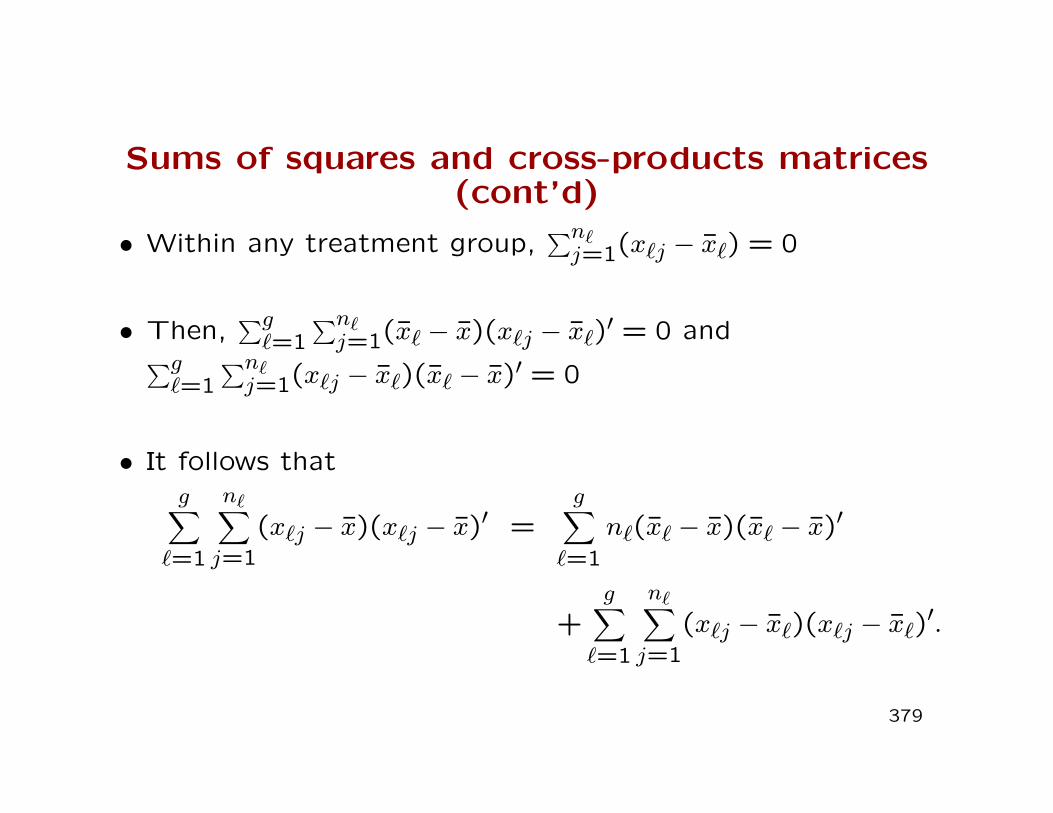
Sums of squares and cross-products matrices(cont’d)
• Within any treatment group,∑n`j=1(x`j − x̄`) = 0
• Then,∑g`=1
∑n`j=1(x̄` − x̄)(x`j − x̄`)′ = 0 and∑g
`=1∑n`j=1(x`j − x̄`)(x̄` − x̄)′ = 0
• It follows thatg∑
`=1
n∑̀j=1
(x`j − x̄)(x`j − x̄)′ =g∑
`=1
n`(x̄` − x̄)(x̄` − x̄)′
+g∑
`=1
n∑̀j=1
(x`j − x̄`)(x`j − x̄`)′.
379

Sums of squares and cross-products matrices(cont’d)
• The matrix to the left of the = sign is called the correctedtotal sums of squares and cross products matrix.
• The matrices on the right side are called, respectively, thetreatment sums of squares and cross-products matrix,denoted by B, and the error sums of squares and cross-products matrix, denoted by W (for ’within groups’).
• Notice that we can re-write the W matrix as
W =g∑
`=1
n∑̀j=1
(x`j − x̄`)(x`j − x̄`)′
= (n1 − 1)S1 + (n2 − 1)S2 + · · ·+ (ng − 1)Sg.
380
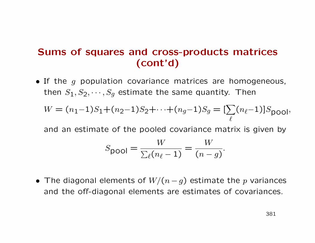
Sums of squares and cross-products matrices(cont’d)
• If the g population covariance matrices are homogeneous,
then S1, S2, · · · , Sg estimate the same quantity. Then
W = (n1−1)S1+(n2−1)S2+· · ·+(ng−1)Sg = [∑`
(n`−1)]Spool,
and an estimate of the pooled covariance matrix is given by
Spool =W∑
`(n` − 1)=
W
(n− g).
• The diagonal elements of W/(n− g) estimate the p variances
and the off-diagonal elements are estimates of covariances.
381

Sums of squares and cross-products matrices(cont’d)
• Using the linear model set-up, we can extend some of the
results from linear model theory and note that
B = X ′A(A′A)−1A′X = X ′PAX
W = X ′[I − PA]X,
where PA = A(A′A)−1A′ is the usual idempotent projection
matrix.
382

Hypotheses Testing in MANOVA
• We often wish to test H0 : τ1 = τ2 = · · · = τg versusH1 : At least two τ ′`s are not equal.
• Compare the relative sizes of B and W .
Source of Matrix of sum of squares and Degrees ofvariation cross-products (SSP) freedom (d.f.)
Treatment B =∑` n`(x̄` − x̄)(x̄` − x̄)′ g − 1
Residual W =∑`∑j(x`j − x̄`)(x`j − x̄`)′ n− g
Total corrected B +W =∑`∑j(x`j − x̄)(x`j − x̄)′ n− 1
383
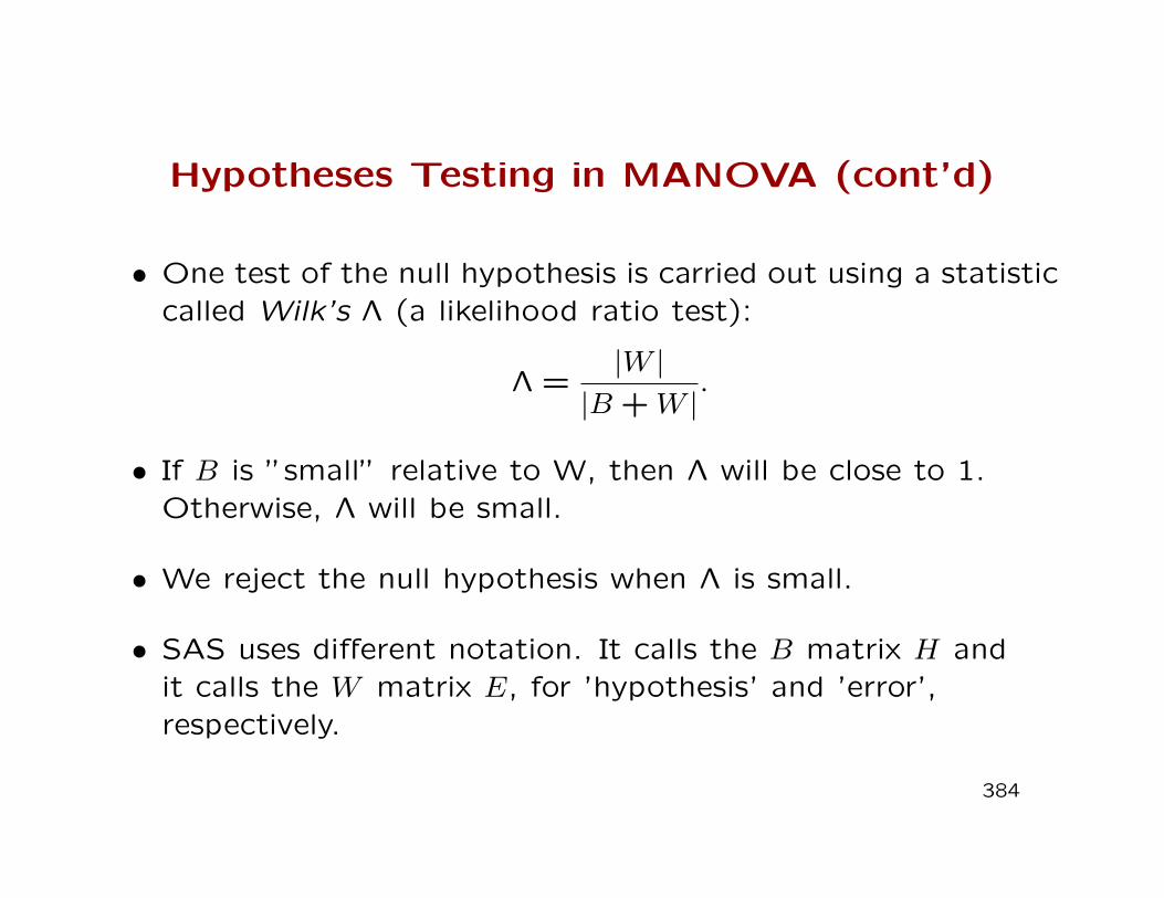
Hypotheses Testing in MANOVA (cont’d)
• One test of the null hypothesis is carried out using a statisticcalled Wilk’s Λ (a likelihood ratio test):
Λ =|W |
|B +W |.
• If B is ”small” relative to W, then Λ will be close to 1.Otherwise, Λ will be small.
• We reject the null hypothesis when Λ is small.
• SAS uses different notation. It calls the B matrix H andit calls the W matrix E, for ’hypothesis’ and ’error’,respectively.
384

Hypotheses Testing in MANOVA (cont’d)
• The exact sampling distribution of Wilk’s Λ can be derived
only for special cases (see next page).
• In general, for large n and under H0, Bartlett showed that
−(n− 1−
(p+ g)
2
)ln Λ ∼ χ2
p(g−1),
where the distribution is approximate. Thus, we reject H0 at
level α when
−(n− 1−
(p+ g)
2
)ln Λ ≥ χ2
p(g−1)(α).
385

Exact distribution of Wilk’s Λ
No. of No. of Sampling distribution for multivariatevariables groups normal data
p = 1 g ≥ 2(n−gg−1
) (1−Λ
Λ
)∼ Fg−1,n−g
p = 2 g ≥ 2(n−g−1g−1
) (1−√
Λ√Λ
)∼ F2(g−1),2(n−g−1)
p ≥ 1 g = 2(n−p−1
p
) (1−Λ
Λ
)∼ Fp,n−p−1
p ≥ 1 g = 3(n−p−2
p
) (1−√
Λ√Λ
)∼ F2p,2(n−p−2)
386
Other Tests
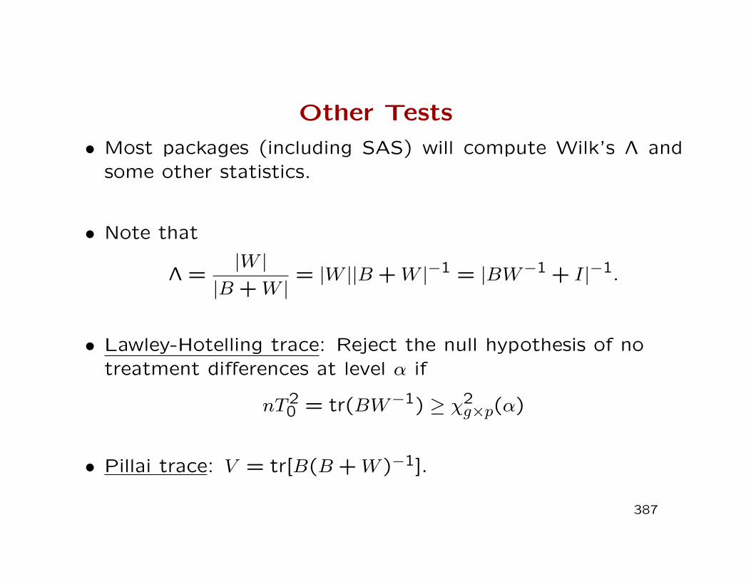
• Most packages (including SAS) will compute Wilk’s Λ andsome other statistics.
• Note that
Λ =|W |
|B +W |= |W ||B +W |−1 = |BW−1 + I|−1.
• Lawley-Hotelling trace: Reject the null hypothesis of notreatment differences at level α if
nT20 = tr(BW−1) ≥ χ2
g×p(α)
• Pillai trace: V = tr[B(B +W )−1].
387

Other Tests
• Roy’s maximum root: the test statistic is the largest
eigenvalue of BW−1. (The F-distribution used by SAS is not
accurate.)
• The power of Wilk’s, Lawley-Hotelling and Pillai statistics is
similar. Roy’s statistic has higher power only when one of
the g treatments is very different from the rest.
• Limited simulation results suggest that Pillai’s trace may be
slightly more robust to departures from multivariate normal-
ity.
388


